Abstract

In good arm identification (GAI), the goal is to identify one arm whose average performance exceeds a given threshold, referred to as good arm, if it exists. Few works have studied GAI in the fixed-budget setting, when the sampling budget is fixed beforehand, or the anytime setting, when a recommendation can be asked at any time. We propose APGAI, an anytime and parameter-free sampling rule for GAI in stochastic bandits. APGAI can be straightforwardly used in fixed-confidence and fixed-budget settings. First, we derive upper bounds on its probability of error at any time. They show that adaptive strategies are more efficient in detecting the absence of good arms than uniform sampling. Second, when APGAI is combined with a stopping rule, we prove upper bounds on the expected sampling complexity, holding at any confidence level. Finally, we show good empirical performance of APGAI on synthetic and real-world data. Our work offers an extensive overview of the GAI problem in all settings.

1 INTRODUCTION

Multi-armed bandit algorithms are a family of approaches which demonstrated versatility in solving online allocation problems, where constraints are set on the possible allocations: e.g.  randomized clinical trials (Thompson,, 1933; Berry,, 2006), hyperparameter optimization (Li et al.,, 2017; Shang et al.,, 2018), or active learning (Carpentier et al.,, 2011). The agents face a black-box environment, upon which they can sequentially act through actions, called arms. After sampling an arm $a\in\mathcal{A}$, they receive output from the environment through a scalar observation, which is a realization from the unknown probability distribution $\nu_{a}$ of arm $a$ whose mean will be denoted by $\mu_{a}$. Depending on their objectives, agents should have different sampling strategies.

In pure exploration problems, the goal is to answer a question about the set of arms. It has been studied in two major theoretical frameworks (Audibert et al.,, 2010; Gabillon et al.,, 2012; Jamieson and Nowak,, 2014; Garivier and Kaufmann,, 2016): the fixed-confidence and fixed-budget setting. In the fixed-confidence setting, the agent aims at minimizing the number of samples used to identify a correct answer with confidence $1-\delta$. In the fixed-budget setting, the objective is to minimize the probability of misidentifying a correct answer with a fixed number of samples $T$.

While the constraint on $\delta$ or $T$ is supposed to be given, properly choosing it is challenging for the practitioner since a “good” choice typically depends on unknown quantities. Moreover, in medical applications (e.g.  clinical trials or outcome scoring), the maximal budget is limited but might not be fixed beforehand. When the collected data shows sufficient evidence in favor of one answer, an experiment is often stopped before the initial budget is reached, referred to as early stopping. When additional sampling budget have been obtained due to new funding, an experiment can continue after the initial budget has been consumed, referred to as continuation. While early stopping and continuation are common practices, both fixed-confidence and fixed-budget settings fail to provide useful guarantees for them. Recently, the anytime setting has received increased scrutiny as it fills this gap between theory and practice. In the anytime setting, the agent aims at achieving a low probability of error at any deterministic time (Jun and Nowak,, 2016; Zhao et al.,, 2023; Jourdan et al., 2023b, ). When the candidate answer has anytime guarantees, the practitioners can use continuation or early stopping (when combined with a stopping rule).

The most studied topic in pure exploration is the best arm (BAI) / Top-$m$ identification problem, which aims at determining a subset of $m$ arms with largest means (Karnin et al.,, 2013; Xu et al.,, 2018; Tirinzoni and Degenne,, 2022). However, in some applications such as investigating treatment protocols, BAI requires too many samples for it to be useful in practice. To avoid wasteful queries, practitioners might be interested in easier tasks that identify one “good enough” option. For instance, in $\varepsilon$-BAI (Mannor and Tsitsiklis,, 2004; Even-Dar et al.,, 2006; Garivier and Kaufmann,, 2021; Jourdan et al., 2023b, ), the agent is interested in an arm which is $\varepsilon$-close to the best one, i.e.  $\mu_{a}\geq\max_{k\in\mathcal{A}}\mu_{k}-\varepsilon$. The larger $\varepsilon$ is, the easier the task. However, choosing a meaningful value of $\varepsilon$ can be tricky. This is why the focus of this paper is good arm identification (GAI), where the agent aims to obtain a good arm, which is defined as an arm whose average performance exceeds a given threshold $\theta$, i.e.  $\mu_{a}\geq\theta$. For instance, in our outcome scoring problem (see Section 5), practitioners have enough information about the distributions to define a meaningful threshold beforehand. GAI and variants have been studied in the fixed-confidence setting (Kaufmann et al.,, 2018; Kano et al.,, 2019; Tabata et al.,, 2020), but algorithms for fixed-budget or anytime GAI are missing despite their practical relevance. In this paper, we fill this gap by introducing APGAI, an anytime and parameter-free sampling rule for GAI which is independent of a budget $T$ or a confidence $\delta$ and can be used in the fixed-budget and fixed-confidence settings.

1.1 Problem Statement

We denote by $\mathcal{D}$ a set to which the distributions of the arms are known to belong. We suppose that all distributions in $\mathcal{D}$ are $\sigma$-sub-Gaussian. A distribution $\nu_{0}$ is $\sigma$-sub-Gaussian of mean $\mu_{0}$ if it satisfies $\mathbb{E}_{X\sim\nu_{0}}[e^{\lambda(X-\mu_{0})}]\leq e^{\sigma^{2}\lambda^{2}/2}$ for all $\lambda\in\mathbb{R}$. By rescaling, we assume $\sigma_{a}=1$ for all $a\in\mathcal{A}$. Let $\mathcal{A}$ be the set of arms of size $K$. A bandit instance is defined by unknown distributions $\nu:=(\nu_{a})_{a\in\mathcal{A}}\in\mathcal{D}^{K}$ with means $\mu:=(\mu_{a})_{a\in\mathcal{A}}\in\mathbb{R}^{K}$. Given a threshold $\theta\in\mathbb{R}$, the set of good arms is defined as $\mathcal{A}_{\theta}(\mu):=\left\{a\in\mathcal{A}\mid\mu_{a}\geq\theta\right\}$, which we shorten to $\mathcal{A}_{\theta}$ when $\mu$ is unambiguous. In the remainder of the paper, we assume that $\mu_{a}\neq\theta$ for all $a\in\mathcal{A}$. Let the gap of arm $a$ compared to $\theta$ be $\Delta_{a}:=|\mu_{a}-\theta|>0$. Let $\Delta_{\min}=\min_{a\in\mathcal{A}}\Delta_{a}$ be the minimum gap over all arms. Let

$$H_{1}(\mu):=\sum_{a\in\mathcal{A}}\Delta_{a}^{-2}\quad\text{and}\quad H_{\theta}(\mu):=\sum_{a\in\mathcal{A}_{\theta}(\mu)}\Delta_{a}^{-2}\>.$$ (1)

At time $t$, the agent chooses an arm $a_{t}\in\mathcal{A}$ based on past observations and receives a sample $X_{a_{t},t}$, random variable with conditional distribution $\nu_{a_{t}}$ given $a_{t}$. Let $\mathcal{F}_{t}:=\sigma(a_{1},X_{a_{1},1},\cdots,a_{t},X_{a_{t},t})$ be the $\sigma$-algebra, called history, which encompasses all the information available to the agent after $t$ rounds.

Identification Strategy

In the anytime setting, an identification strategy is defined by two rules which are $\mathcal{F}_{t}$-measurable at time $t$: a sampling rule $a_{t+1}\in\mathcal{A}$ and a recommendation rule $\hat{a}_{t}\in\mathcal{A}\cup\{\emptyset\}$. In GAI, the probability of error $P^{\text{err}}_{\nu,\mathfrak{A}}(t):=\mathbb{P}_{\nu}(\mathcal{E}^{\text{err}}_{\mathfrak{A}}(t))$ of algorithm $\mathfrak{A}$ on instance $\mu$ at time $t$ is the probability of the error event $\mathcal{E}^{\text{err}}_{\mathfrak{A}}(t)=\{\hat{a}_{t}\in\{\emptyset\}\cup(\mathcal{A}\setminus\mathcal{A}_{\theta})\}$ when $\mathcal{A}_{\theta}\neq\emptyset$, otherwise $\mathcal{E}^{\text{err}}_{\mathfrak{A}}(t)=\{\hat{a}_{t}\neq\emptyset\}$ when $\mathcal{A}_{\theta}=\emptyset$.

Those rules have a different objective depending on the considered setting. In anytime GAI, they are designed to ensure that $P^{\text{err}}_{\nu,\mathfrak{A}}(t)$ is small at any time $t$. In fixed-budget GAI, the goal is to have a low $P^{\text{err}}_{\nu,\mathfrak{A}}(T)$, where $T$ is fixed beforehand. Whereas in fixed-confidence GAI, these two rules are complemented by a stopping rule using a confidence level $1-\delta$ fixed beforehand such that $\mathfrak{A}$ stops sampling after $\tau_{\delta}$ rounds. The stopping time $\tau_{\delta}$ is also known as the sample complexity of a fixed-confidence algorithm. At stopping time $\tau_{\delta}$, the algorithm should satisfy $\delta$-correctness, which means that $\mathbb{P}_{\nu}(\{\tau_{\delta}<+\infty\}\cap\mathcal{E}^{\text{err}}_{\mathfrak{A}}(\tau_{\delta}))\leq\delta$ for all instances $\mu$. That requirement leads to a lower bound on the expected sample complexity on any instance. The following lemma is similar to other bounds derived in various settings linked to GAI (Kaufmann et al.,, 2018; Tabata et al.,, 2020). The proof in Appendix E.1 relies on the well-known change of measure inequality (Kaufmann et al.,, 2016, Lemma $1$).

Lemma 1.

Let $\delta\in(0,1)$. For all $\delta$-correct strategy and all Gaussian instances $\nu_{a}=\mathcal{N}(\mu_{a},1)$ with $\mu_{a}\neq\theta$, we have $\liminf_{\delta\to 0}\mathbb{E}_{\nu}[\tau_{\delta}]/\log(1/\delta)\geq T^{\star}(\mu)$, where

$$T^{\star}(\mu):=\begin{cases}2\min_{a\in\mathcal{A}_{\theta}(\mu)}\Delta_{a}^{-2}&\text{if }\mathcal{A}_{\theta}(\mu)\neq\emptyset\;,\\ 2H_{1}(\mu)&\text{otherwise}\;.\end{cases}$$ (2)

A fixed-confidence algorithm is said to be asymptotically optimal if it is $\delta$-correct, and its expected sample complexity matches the lower bound, i.e.  $\limsup_{\delta\to 0}\mathbb{E}_{\nu}[\tau_{\delta}]/\log(1/\delta)\leq T^{\star}(\mu)$.

1.2 Contributions

We propose APGAI, an anytime and parameter-free sampling rule for GAI in stochastic bandits, which is independent of a budget $T$ or a confidence $\delta$. APGAI is the first algorithm which can be employed without modification for fixed-budget GAI (and without prior knowledge of the budget) and fixed-confidence GAI. Furthermore, it enjoys guarantees in both settings. As such, APGAI allows both continuation and early stopping. First, we show an upper bound on $P^{\text{err}}_{\nu,\text{APGAI}}(t)$ of the order $\exp(-\mathcal{O}(t/H_{1}(\mu)))$ which holds for any deterministic time $t$ (Theorem 1). Adaptive strategies are more efficient in detecting the absence of good arms than uniform sampling (see Section 3). Second, when combined with a GLR stopping rule, we derive an upper bound on $\mathbb{E}_{\nu}[\tau_{\delta}]$ holding at any confidence level (Theorem 2). In particular, APGAI is asympotically optimal for GAI with Gaussian distributions when there is no good arm. Finally, APGAI is easy to implement, computationally inexpensive and achieves good empirical performance in both settings on synthetic and real-world data with an outcome scoring problem for RNA-sequencing data (see Section 5). Our work offers an overview of the GAI problem in all settings.

1.3 Related Work

GAI has never been studied in the fixed-budget or anytime setting. In the fixed-confidence setting, several questions have been studied which are closely connected to GAI. Given two thresholds $\theta_{L}<\theta_{U}$, Tabata et al., (2020) studies the Bad Existence Checking problem, in which the agent should output “negative” if $\mathcal{A}_{\theta_{L}}(\mu)=\emptyset$ and “positive” if $\mathcal{A}_{\theta_{U}}(\mu)\neq\emptyset$. They propose an elimination-based meta-algorithm called BAEC, and analyze its expected sample complexity when combined with several index-policy to define the sampling rule.  Kano et al., (2019) considers identifying the whole set of good arms $\mathcal{A}_{\theta}(\mu)$ with high probability, and returns the good arms in a sequential way. We refer to that problem as AllGAI. In Kano et al., (2019), they introduce three index-based GAI algorithms named APT-G, HDoC and LUCB-G, and show upper bounds on their expected sample complexity. A large number of algorithms from previously mentioned works bear a passing resemblance to the APT algorithm in Locatelli et al., (2016) which tackles the thresholding bandit problem in the fixed-budget setting. The latter should classify all arms into $\mathcal{A}_{\theta}$ and $\mathcal{A}_{\theta}^{\complement}$ at the end of the sampling phase. This resemblance lies in that those algorithms rely on an arm index for sampling. The arm indices in BAEC (Tabata et al.,, 2020), APT-G, HDoC and LUCB-G Kano et al., (2019) are reported in Algorithm 2 in Appendix D.

Degenne and Koolen, (2019) addressed the “any low arm” problem, which is a GAI problem for threshold $-\theta$ on instance $-\mu$. They introduce Sticky Track-and-Stop, which is asymptotically optimal in the fixed-confidence setting. In Kaufmann et al., (2018), the “bad arm existence” problem aims to answer “no” when $\mathcal{A}_{-\theta}(-\mu)=\emptyset$, and “yes” otherwise. They propose an adaptation of Thompson Sampling performing some conditioning on the “worst event” (named Murphy Sampling). The empirical pulling proportions are shown to converge towards the allocation realizing $T^{\star}(\mu)$ in Lemma 1. Another related framework is the identification with high probability of $k$ arms from $\mathcal{A}_{\theta}(\mu)$ (Katz-Samuels and Jamieson,, 2020). They introduce the unverifiable sample complexity. It is the minimum number of samples after which the algorithm always outputs a correct answer with high probability. It does not require to certify that the output is correct.

2 ANYTIME PARAMETER-FREE SAMPLING RULE

We propose the APGAI (Anytime Parameter-free GAI) algorithm, which is independent of a budget $T$ or a confidence $\delta$ and is summarized in Algorithm 1.

Notation

Let $N_{a}(t)=\sum_{s\leq t}\mathds{1}\left(a_{s}=a\right)$ be the number of times arm $a$ is sampled at the end of round $t$, and $\hat{\mu}_{a}(t)=\frac{1}{N_{a}(t)}\sum_{s\leq t}\mathds{1}\left(a_{s}=a\right)X_{a,s}$ be its empirical mean. For all $a\in\mathcal{A}$ and all $t\geq K$, let us define

$$W^{+}_{a}(t)=\sqrt{N_{a}(t)}\Delta_{a}(t)_{+},\ W^{-}_{a}(t)=\sqrt{N_{a}(t)}(-\Delta_{a}(t))_{+}$$ (3)

where $(x)_{+}:=\max(x,0)$ and $\Delta_{a}(t):=\hat{\mu}_{a}(t)-\theta$. If arm $a$ were a $\sigma_{a}$-sub-Gaussian distribution, the rescaling boils down to using $\Delta_{a}(t)/\sigma_{a}$ instead of $\Delta_{a}(t)$. This empirical transportation cost $W^{+}_{a}(t)$ (resp. $W^{-}_{a}(t)$) represents the amount of information collected so far in favor of the hypothesis that $\{\mu_{a}>\theta\}$ (resp. $\{\mu_{a}<\theta\}$). It is linked with the generalized likelihood ratio (GLR) as detailed in Appendix E.2. As initialization, we pull each arm $n_{0}\in\mathbb{N}$ times, and we use $n_{0}=1$.

Algorithm 1 APGAI

1:  Input: threshold $\theta$, set of arms $\mathcal{A}$

2:  Update: empirical means $\hat{\mu}(t)$ and empirical transportation costs $W^{\pm}_{a}(t)$ as in (3)

3:  if $\max_{a\in\mathcal{A}}\hat{\mu}_{a}(t)\leq\theta$ then

4:     $\hat{a}_{t}:=\emptyset$ and $a_{t+1}\in\arg\,\min_{a\in\mathcal{A}}W^{-}_{a}(t)$

5:  else

6:     $\hat{a}_{t}:=a_{t+1}\in\arg\,\max_{a\in\mathcal{A}}W^{+}_{a}(t)$

7:  end

8:  return  arm to pull $a_{t+1}$ and recommendation $\hat{a}_{t}$

Recommendation Rule

At time $t+1>n_{0}K$, the recommendation rule depends on whether the highest empirical mean lies below the threshold $\theta$ or not. When $\max_{a\in\mathcal{A}}\hat{\mu}_{a}(t)\leq\theta$, we recommend the empty set, i.e.  $\hat{a}_{t}=\emptyset$. Otherwise, our candidate answer is the arm which is the most likely to be a good arm given the collected evidence, i.e.  $\hat{a}_{t}\in\arg\,\max_{a\in\mathcal{A}}W^{+}_{a}(t)$.

Sampling Rule

The next arm to pull is based on the APT_P indices introduced by (Tabata et al.,, 2020) as a modification to the APT indices (Locatelli et al.,, 2016). At time $t+1>n_{0}K$, we pull arm $a_{t+1}\in\arg\,\max_{a\in\mathcal{A}}\sqrt{N_{a}(t)}(\hat{\mu}_{a}(t)-\theta)$. To emphasize the link with our recommendation rule, this sampling rule can also be written as $a_{t+1}\in\arg\,\min_{a\in\mathcal{A}}W^{-}_{a}(t)$ when $\max_{a\in\mathcal{A}}\hat{\mu}_{a}(t)\leq\theta$, and $a_{t+1}\in\arg\,\max_{a\in\mathcal{A}}W^{+}_{a}(t)$ otherwise. Ties are broken arbitrarily at random, up to the constraint that $\hat{a}_{t}=a_{t+1}$ when $\max_{a\in\mathcal{A}}\hat{\mu}_{a}(t)>\theta$. This formulation better highlights the dual behavior of APGAI. When $\max_{a\in\mathcal{A}}\hat{\mu}_{a}(t)\leq\theta$, APGAI collects additional observations to verify that there are no good arms, hence pulling the arm which is the least likely to not be a good arm. Otherwise, APGAI gathers more samples to confirm its current belief that there is at least one good arm, hence pulling the arm which is the most likely to be a good arm.

Memory and Computational Cost

APGAI needs to maintain in memory the values $N_{a}(t),\hat{\mu}_{a}(t),W^{\pm}_{a}(t)$ for each arm $a\in\mathcal{A}$, hence the total memory cost is in $\mathcal{O}(K)$. The computational cost of APGAI is in $\mathcal{O}(K)$ per iteration, and its update cost is in $\mathcal{O}(1)$.

Differences to BAEC

While both APGAI and BAEC(APT_P) rely on the APT_P indices (Tabata et al.,, 2020), they differ significantly. BAEC is an elimination-based meta-algorithm which samples active arms and discards arms whose upper confidence bounds (UCB) on the empirical means are lower than $\theta_{U}$. The recommendation rule of BAEC is only defined at the stopping time, and it depends on lower confidence bounds (LCB) and UCB. Since the UCB/LCB indices depend inversely on the gap $\theta_{U}-\theta_{L}>0$ and on the confidence $\delta$, BAEC is neither anytime nor parameter-free. More importantly, APGAI can be used without modification for fixed-confidence or fixed-budget GAI. In contrast, BAEC can solely be used in the fixed-confidence setting when $\theta_{U}>\theta_{L}$, hence not for GAI itself (i.e.  $\theta_{U}=\theta_{L}$).

3 ANYTIME GUARANTEES ON THE PROBABILITY OF ERROR

To allow continuation or (deterministic) early stopping, the candidate answer of APGAI should be associated with anytime theoretical guarantees. Theorem 1 shows an upper bound of the order $\exp(-\mathcal{O}(t/H_{1}(\mu)))$ for $P^{\text{err}}_{\nu,\mathfrak{A}}(t)$ that holds for any deterministic time $t$.

Theorem 1.

Let $p(x)=x-0.5\log x$. The APGAI algorithm $\mathfrak{A}$ satisfies that, for all $\nu\in\mathcal{D}^{K}$ with mean $\mu$ such that $\Delta_{\min}>0$, for all $t>n_{0}K+2|\mathcal{A}_{\theta}|$,

$$P^{\text{err}}_{\nu,\mathfrak{A}}(t)\leq Ke\sqrt{2}\log(e^{2}t)\exp\left(-p\left(\frac{t-n_{0}K-2|\mathcal{A}_{\theta}|}{2\alpha_{i_{\mu}}H_{1}(\mu)}\right)\right)$$

where $H_{1}(\mu)$ as in (1), $(\alpha_{1},\alpha_{\theta})=(9,2)$ and $i_{\mu}=1+(\theta-1)\mathds{1}\left(\mathcal{A}_{\theta}(\mu)\neq\emptyset\right)$.

Theorem 1 holds for any deterministic time $t>n_{0}K+2|\mathcal{A}_{\theta}|$ and any $1$-sub-Gaussian instance $\nu$. In the asymptotic regime where $t\to+\infty$, Theorem 1 shows that $\limsup_{t\rightarrow+\infty}t\log(1/P^{\text{err}}_{\nu,\mathfrak{A}}(t))^{-1}\leq 2\alpha_{i_{\mu}}H_{1}(\mu)$ for APGAI with $(\alpha_{1},\alpha_{\theta})=(9,2)$. We defer the reader to Appendix H for a detailed proof.

Comparison With Uniform Sampling

Despite the practical relevance of anytime and fixed-budget guarantees, APGAI is the first algorithm enjoying guarantees on the probability of error in GAI at any time $t$ (hence at a given budget $T$). As baseline, we consider the uniform round-robin algorithm, named Unif, which returns the best empirical arm at time $t$ if its empirical mean is higher than $\theta$, and returns $\emptyset$ otherwise. At time $t$ such that $t/K\in\mathbb{N}$, the recommendation of Unif is equivalent to the one used in APGAI, i.e.  $\arg\,\max_{a\in\mathcal{A}}W^{+}_{a}(t)=\arg\,\max_{a\in\mathcal{A}}\hat{\mu}_{a}(t)$ since $N_{a}(t)=t/K$. As the two algorithms only differ by their sampling rule, we can measure the benefits of adaptive sampling. Theorem 4 in Appendix C gives anytime upper bounds on $P^{\text{err}}_{\nu,\text{Unif}}(t)$. In the asymptotic regime, Unif achieves a rate in $2K\Delta_{\min}^{-2}$ when $\mathcal{A}_{\theta}(\mu)=\emptyset$, and $4K\min_{a\in\mathcal{A}_{\theta}(\mu)}\Delta_{a}^{-2}$ otherwise. While the latter rate is better than $2H_{1}(\mu)$ when arms have dissimilar gaps, APGAI has better guarantees than Unif when there is no good arm. Our experiments shows that APGAI outperforms Unif on most instances (e.g.  Figures 1 and 2), and is on par with it otherwise.

Worst-case Lower Bound

Degenne, (2023) recently studied the existence of a complexity in fixed-budget pure exploration. While there is a complexity $T^{\star}(\mu)$ as in (2) for the fixed-confidence setting, (Degenne,, 2023, Theorem $6$) shows that a sequence of fixed-budget algorithms $(\mathfrak{A}_{T})_{T}$ (where $\mathfrak{A}_{T}$ denotes the algorithm using fixed budget $T$) cannot have a better asymptotic rate than $KT^{\star}(\mu)$ on all Gaussian instances

$$\exists\mu\in\mathbb{R}^{K},\ \limsup_{T\to+\infty}T\log(1/P^{\text{err}}_{\nu,\mathfrak{A}_{T}}(T))^{-1}\geq KT^{\star}(\mu)\>.$$ (4)

Unif achieves the rate $KT^{\star}(\mu)$ when $\mathcal{A}_{\theta}\neq\emptyset$, but suffers from worse guarantees otherwise. Conversely, APGAI achieves the rate in $T^{\star}(\mu)$ when $\mathcal{A}_{\theta}=\emptyset$, but has sub-optimal guarantees otherwise. It does not conflict with (4) e.g.  considering $\mu$ with $\mathcal{A}_{\theta}\neq\emptyset$ and such that there exists an arm $a\in\mathcal{A}$ with $\Delta_{a}\leq\max_{a\in\mathcal{A}_{\theta}}\Delta_{a}/\sqrt{K/2-1}$. Experiments in Section 5 suggest that the sub-optimal dependency when $\mathcal{A}_{\theta}\neq\emptyset$ is not aligned with the good practical performance of APGAI. Formally proving better guarantees when $\mathcal{A}_{\theta}(\mu)\neq\emptyset$ is a direction for future work.

In fixed-budget GAI, a good strategy has highly different sampling modes depending on whether there is a good arm or not. Since wrongfully committing to one of those modes too early will incur higher error, it is challenging to find the perfect trade-off in an adaptive manner. Designing an algorithm whose guarantees are comparable to (4) for all instances is an open problem.

3.1 Benchmark: Other GAI Algorithms

To go beyond the comparison with Unif, we propose and analyze additional GAI algorithms. A summary of the comparison with APGAI is shown in Table 1.

3.1.1 From BAI to GAI Algorithms

Since a BAI algorithm outputs the arm with highest mean, it can be adapted to GAI by comparing the mean of the returned arm to the known threshold. We study the GAI adaptations of two fixed-budget BAI algorithms: Successive Rejects (SR) (Audibert et al.,, 2010) and Sequential Halving (SH) (Karnin et al.,, 2013). SR-G and SH-G return $\hat{a}_{T}=\emptyset$ when $\hat{\mu}_{a_{T}}(T)\leq\theta$ and $\hat{a}_{T}=a_{T}$ otherwise, where $a_{T}$ is the arm that would be recommended for the BAI problem, i.e.  the last arm that was not eliminated.

Theorems 5 and 6 in Appendix C give an upper bound on $P^{\text{err}}_{\nu,\text{SR-G}}(T)$ and $P^{\text{err}}_{\nu,\text{SH-G}}(T)$ at the fixed budget $T$. In the asymptotic regime, their rate is in $4\log(K)\Delta_{\min}^{-2}$ when $\mathcal{A}_{\theta}(\mu)=\emptyset$, otherwise

$$\mathcal{O}(\log(K)\max\{\max_{a\in\mathcal{A}_{\theta}}\Delta_{a}^{-2},\max_{i>I^{\star}}i(\max_{a\in\mathcal{A}}\mu_{a}-\mu_{(i)})^{-2}\})$$

with $I^{\star}=|\arg\,\max_{a\in\mathcal{A}}\mu_{a}|$ and $\mu_{(i)}$ be the $i^{\text{th}}$ largest mean in vector $\mu$. Recently, Zhao et al., (2023) have provided a finer analysis of SH. Using their result yields mildly improved rates. We defer the reader to Appendix C for further details. Those rates are better than $2H_{1}(\mu)$ when there is one good arm with large mean and the remaining arms have means slightly smaller than $\theta$. However, APGAI has better guarantees than SR-G and SH-G when there is one good arm with mean slightly smaller than the largest mean.

Doubling Trick

The doubling trick allows the conversion of any fixed-budget algorithm into an anytime algorithm. It considers a sequences of algorithms that are run with increasing budgets $(T_{k})_{k\geq 1}$, and recommends the answer outputted by the last instance.  Zhao et al., (2023) shows that Doubling SH obtains the same guarantees than SH in BAI, hence Theorem 5 also holds for its GAI counterpart DSH-G (resp. Theorem 6 for DSR-G) at the cost of a multiplicative factor $4$ in the rate. Empirically, our experiments show that APGAI is always better than DSR-G and DSH-G (Fig. 1 and 2).

Table 1: Asymptotic error rate $C(\mu)$ of algorithm $\mathfrak{A}$ on $\nu$, i.e.  $\limsup_{t}t\log(1/P^{\text{err}}_{\nu,\mathfrak{A}}(t))^{-1}\leq C(\mu)$. $(\dagger)$ Fixed-budget algorithm $\mathfrak{A}_{T,\nu}$ with prior knowledge on $\nu$. $H_{1}(\mu)$ as in (1), $\Delta_{\min}:=\min_{a\in\mathcal{A}}\Delta_{a}$, $\overline{\Delta}_{\max}:=\max_{a\in\mathcal{A}_{\theta}}\Delta_{a}$, $I^{\star}=|\arg\,\max_{a\in\mathcal{A}}\mu_{a}|$ and $\widetilde{\Delta}^{-2}:=\max\{\max_{a\in\mathcal{A}_{\theta}}\Delta_{a}^{-2},\max_{i>I^{\star}}i(\max_{a\in\mathcal{A}}\mu_{a}-\mu_{(i)})^{-2}\}$.

Algorithm $\mathfrak{A}$	$\mathcal{A}_{\theta}(\mu)=\emptyset$	$\mathcal{A}_{\theta}(\mu)\neq\emptyset$
APGAI [Th. 1]	$18H_{1}(\mu)$	$4H_{1}(\mu)$
Unif [Th. 4]	$2K\Delta_{\min}^{-2}$	$4K\overline{\Delta}_{\max}^{-2}$
DSR-G [Th. 5]	$16\log K\Delta_{\min}^{-2}$	$4\log K\widetilde{\Delta}^{-2}$
DSH-G [Th. 6]	$16\log K\Delta_{\min}^{-2}$	$4\log K\widetilde{\Delta}^{-2}$
PKGAI($\star$) [Th. 7]$\dagger$	$2H_{1}(\mu)$	$2H_{1}(\mu)$
PKGAI(Unif) [Th. 8]$\dagger$	$2H_{1}(\mu)$	$2K\hat{\Delta}^{-2}$

3.1.2 Prior Knowledge-based GAI Algorithms

Several fixed-budget BAI algorithms assume that the agent has access to some prior knowledge on unknown quantities to design upper/lower confidence bounds (UCB/LCB), e.g.  UCB-E (Audibert et al.,, 2010) and UGapEb (Gabillon et al.,, 2012). While this assumption is often not realistic, it yields better guarantees. We investigate those approaches for fixed-budget GAI. We propose an elimination-based meta-algorithm for fixed-budget GAI called PKGAI (Prior Knowledge-based GAI), described in Appendix D. As for BAEC, PKGAI($\star$) takes as input an index policy $\star$ which is used to define the sampling rule. The main difference to BAEC lies in the definition of the UCB/LCB since they depend both on the budget $T$ and on knowledge of $H_{1}(\mu)$ and $H_{\theta}(\mu)$.

We provide upper confidence bounds on the probability of error at time $T$ holding for any choice of indices (Theorem 7 for PKGAI($\star$)) and for uniform round-robin sampling (Theorem 8 for PKGAI(Unif)). The obtained upper bounds on $P^{\text{err}}_{\nu,\text{PKGAI}}(T)$ are marginally lower than the ones obtained for APGAI, while APGAI does not require the knowledge of $H_{1}(\mu)$ and $H_{\theta}(\mu)$.

3.2 Unverifiable Sample Complexity

The unverifiable sample complexity was defined in Katz-Samuels and Jamieson, (2020) as the smallest stopping time $\tau_{U,\delta}$ after which an algorithm always outputs a correct answer with probability at least $1-\delta$. In GAI, this means that algorithm $\mathfrak{A}$ satisfies $\mathbb{P}_{\nu}(\bigcup_{t\geq\tau_{U,\delta}}\mathcal{E}^{\text{err}}_{\mathfrak{A}}(t))\leq\delta$. Compared to the fixed-confidence setting, it does not require to certify that the candidate answer is correct. Authors in Zhao et al., (2023) notice that anytime bounds on the error can imply an unverifiable sample complexity bound. Theorem 3 in Appendix B.3 gives a deterministic upper bound on the unverifiable sample complexity $\tau_{U,\delta}$ of APGAI, i.e.

$U_{\delta}(\mu)=_{\delta\to 0}2\alpha_{i_{\mu}}H_{1}(\mu)\log(1/\delta)+\mathcal{O}(\log\log(1/\delta))\>$

with $i_{\mu}=1+(\theta-1)\mathds{1}\left(\mathcal{A}_{\theta}(\mu)\neq\emptyset\right)$ and $(\alpha_{1},\alpha_{\theta})=(9,2)$. While such upper bounds are known in BAI (Katz-Samuels and Jamieson,, 2020; Zhao et al.,, 2023; Jourdan et al., 2023b, ), this is the first result for GAI.

4 FIXED-CONFIDENCE GUARANTEES

In some applications, the practitioner has a strict constraint on the confidence $\delta$ associated with the candidate answer. This constraint simultaneously supersedes any limitation on the sampling budget and allows early stopping when enough evidence is collected (random since data-dependent). In the fixed-confidence setting, an identification strategy should define a stopping rule in addition of the sampling and recommendation rules.

Stopping Rule

We couple APGAI with the GLR stopping rule (Garivier and Kaufmann,, 2016) for GAI (see Appendix E.2), which coincides with the Box stopping rule introduced in Kaufmann et al., (2018). At fixed confidence $\delta$, we stop at $\tau_{\delta}:=\min(\tau_{>,\delta},\tau_{<,\delta})$

$$\begin{split}\text{where }&\tau_{>,\delta}:=\inf\{t\mid\max_{a\in\mathcal{A}}W^{+}_{a}(t)\geq\sqrt{2c(t,\delta)}\}\>,\\ &\tau_{<,\delta}:=\inf\{t\mid\min_{a\in\mathcal{A}}W^{-}_{a}(t)\geq\sqrt{2c(t,\delta)}\}\>,\end{split}$$ (5)

and $c:\mathbb{N}\times(0,1)\to\mathbb{R}_{+}$ is a threshold function. Proven in Appendix G.1, Lemma 2 gives a threshold ensuring that the GLR stopping rule (5) is $\delta$-correct for all $\delta\in(0,1)$, independently of the sampling rule.

Lemma 2.

Let $\overline{W}_{-1}(x)=-W_{-1}(-e^{-x})$ for all $x\geq 1$, where $W_{-1}$ is the negative branch of the Lambert $W$ function. It satisfies $\overline{W}_{-1}(x)\approx x+\log x$. Let $\delta\in(0,1)$. Given any sampling rule, using the threshold

$$2c(t,\delta)=\overline{W}_{-1}(2\log(K/\delta)+4\log\log(e^{4}t)+1/2)$$ (6)

in the GLR stopping rule (5) yields a $\delta$-correct algorithm for $1$-sub-Gaussian distributions.

Non-asymptotic Upper Bound

Theorem 2 gives an upper bound on the expected sample complexity of the resulting algorithm holding for any confidence $\delta$.

Theorem 2.

Let $\delta\in(0,1)$. Combined with GLR stopping (5) using threshold (6), the APGAI algorithm is $\delta$-correct and it satisfies that, for all $\nu\in\mathcal{D}^{K}$ with mean $\mu$ such that $\Delta_{\min}>0$,

$$\mathbb{E}_{\nu}[\tau_{\delta}]\leq C_{\mu}(\delta)+K\pi^{2}/6+1\>,$$

where $i_{\mu}:=1+(\theta-1)\mathds{1}\left(\mathcal{A}_{\theta}(\mu)\neq\emptyset\right)$ and $C_{\mu}(\delta):=$

$$\sup\{t\mid t\leq 2H_{i_{\mu}}(\mu)(\sqrt{c(t,\delta)}+\sqrt{3\log t})^{2}+D_{i_{\mu}}(\mu)\}\>,$$

with $H_{1}(\mu)$ and $H_{\theta}(\mu)$ as in (1). $D_{1}(\mu)$ and $D_{\theta}(\mu)$ are defined in Lemmas 16 and 18 in Appendix F, satisfying

$$D_{1}(\mu)\approx_{\Delta_{\min}\to+\infty}D_{\theta}(\mu)=\mathcal{O}(H_{1}(\mu)\log H_{1}(\mu))\;.$$

In the asymptotic regime, we obtain

$$\limsup_{\delta\to 0}\mathbb{E}_{\nu}[\tau_{\delta}]/\log(1/\delta)\leq 2H_{i_{\mu}}(\mu)\;.$$

since $C_{\mu}(\delta)=_{\delta\to 0}2H_{i_{\mu}}(\mu)\log(1/\delta)+\mathcal{O}(\log\log(1/\delta))$.

Most importantly, Theorem 2 holds for any confidence $\delta\in(0,1)$ and any $1$-sub-Gaussian instance $\nu$. In the asymptotic regime where $\delta\to 0$, Theorem 2 shows that $\limsup_{\delta\to 0}\mathbb{E}_{\nu}[\tau_{\delta}]/\log(1/\delta)\leq 2H_{i_{\mu}}(\mu)$. This implies that APGAI is asymptotically optimal for Gaussian distributions when $\mathcal{A}_{\theta}=\emptyset$. When there are good arms, our upper bound scales as $H_{\theta}(\mu)\log(1/\delta)$, which is better than the scaling in $H_{1}(\mu)\log(1/\delta)$ obtained for the unverifiable sample complexity.

However, when $\mathcal{A}_{\theta}\neq\emptyset$, our upper bound is sub-optimal compared to $2\min_{a\in\mathcal{A}}\Delta_{a}^{-2}$ (see Lemma 1). This sub-optimal scaling stems from the greediness of APGAI when $\mathcal{A}_{\theta}\neq\emptyset$ since there is no mechanism to detect an arm that is easiest to verify, i.e.  $\arg\,\max_{a\in\mathcal{A}_{\theta}}\Delta_{a}$. Empirically, we observe that APGAI can suffer from large outliers when there are good arms with dissimilar gaps, and that adding forced exploration circumvents this issue (Figure 22 and Table 11 in Appendix I.5). Intuitively, a purely asymptotic analysis of APGAI would yield the dependency $2\max_{a\in\mathcal{A}_{\theta}}\Delta_{a}^{-2}$ which is independent from $|\mathcal{A}_{\theta}|$. This intuition is supported by empirical evidence (Figure 3), and we defer the reader to Appendix F.2.1 for more details. Compared to asymptotic results, our non-asymptotic guarantees hold for reasonable values of $\delta$, with a $\delta$-independent scaling of the order $\mathcal{O}(H_{1}(\mu)\log H_{1}(\mu))$.

Table 2: Asymptotic upper bound $2C(\mu)$ on the expected sample complexity of algorithm $\mathfrak{A}$ on $\nu$, i.e.  $\limsup_{\delta\to 0}\mathbb{E}_{\nu}[\tau_{\delta}]/\log(1/\delta)\leq 2C(\mu)$. ($\mathsection$) Requires an ordering on the possible answers $\mathcal{A}\cup\{\emptyset\}$. $H_{1}(\mu)$ and $H_{\theta}(\mu)$ as in (1), $\overline{\Delta}_{\max}:=\max_{a\mathcal{A}_{\theta}}\Delta_{a}$.

Algorithm $\mathfrak{A}$	$\mathcal{A}_{\theta}(\mu)=\emptyset$	$\mathcal{A}_{\theta}(\mu)\neq\emptyset$
APGAI[Th. 2]	$H_{1}(\mu)$	$H_{\theta}(\mu)$
S-TaS $\mathsection$	$H_{1}(\mu)$	$\overline{\Delta}_{\max}^{-2}$
(Degenne and Koolen,, 2019)
HDoC	$H_{1}(\mu)$	$\overline{\Delta}_{\max}^{-2}$
(Kano et al.,, 2019)
APT-G, LUCB-G	$H_{1}(\mu)$	$-$
(Kano et al.,, 2019)

Comparison With Existing Upper Bounds

Table 2 summarizes the asymptotic scaling of the upper bound on the expected sample complexity of existing GAI algorithms. While most GAI algorithms have better asymptotic guarantees when $\mathcal{A}_{\theta}(\mu)\neq\emptyset$, APGAI is the only one of them which has anytime guarantees on the probability of error (Theorem 1). However, we emphasize that APGAI is not the best algorithm to tackle fixed-confidence GAI since it is designed for anytime GAI. Sticky Track-and-Stop (S-TaS) is asymptotically optimal for the “any low arm” problem (Degenne and Koolen,, 2019), hence for GAI as well. Even though GAI is one of the few setting where S-TaS admits a computationally tractable implementation, its empirical performance heavily relies on the fixed ordering for the set of possible answers (see Table 5 in Appendix I.2). This partly explains the lack of non-asymptotic guarantees for S-TaS which is asymptotic by nature, while APGAI has non-asymptotic guarantees. For the “bad arm existence” problem, Kaufmann et al., (2018) proves that the empirical proportion $(N_{a}(t)/t)_{a\in\mathcal{A}}$ of Murphy Sampling converges almost surely towards the optimal allocation realizing the asymptotic lower bound of Lemma 1. While their result implies that $\lim_{\delta\to 0}\tau_{\delta}/\log(1/\delta)=T^{\star}(\mu)$ almost surely, the authors provide no upper bound on the expected sample complexity of Murphy Sampling. Finally, we consider the AllGAI algorithms introduced in Kano et al., (2019) (HDoC, LUCB-G and APT-G) which enjoy theoretical guarantees for some GAI instances as well. When $\mathcal{A}_{\theta}(\mu)=\emptyset$, all three algorithms have an upper bound of the form $2H_{1}(\mu)\log(1/\delta)+\mathcal{O}(\log\log(1/\delta))$. When $\mathcal{A}_{\theta}(\mu)\neq\emptyset$, only HDoC admits an upper bound on the expected number of time to return one good arm, which is of the form $2\min_{a\in\mathcal{A}_{\theta}}\Delta_{a}^{-2}\log(1/\delta)+\mathcal{O}(\log\log(1/\delta))$.

The indices used for the elimination and recommendation in BAEC (Tabata et al.,, 2020) have a dependence in $\mathcal{O}(-\log(\theta_{U}-\theta_{L}))$, hence BAEC is not defined for GAI where $\theta_{U}=\theta_{L}$. While it is possible to use UCB/LCB which are agnostic to the gap $\theta_{U}-\theta_{L}>0$, these choices have not been studied in Tabata et al., (2020). Extrapolating the theoretical guarantees of BAEC when $\theta_{L}\to\theta_{U}$, one would expect an upper bound on its expected sample complexity of the form $2H_{1}(\mu)\log(1/\delta)+\mathcal{O}((\log(1/\delta))^{2/3})$.

5 EXPERIMENTS

We assess the empirical performance of the APGAI in terms of empirical error, as well as empirical stopping time. Overall, APGAI perform favorably compared to other algorithms in both settings. Moreover, its empirical performance exceeds what its theoretical guarantees would suggest. This discrepancy between theory and practice paves the way for interesting future research. We present a fraction of our experiments, and defer the reader to Appendix I for supplementary experiments.

Outcome Scoring Application

Our real-life motivation is outcome scoring from gene activity (transcriptomic) data. This application is focused on the treatment of encephalopathy of prematurity in infants. The goal is to determine the optimal protocol for the administration of stem cells among $K=18$ realistic possibilities. Our collaborators tested all treatments, and made RNA-related measurements on treated samples. Computed on $3$ technical replicates, the mean value in $[-1,1]$ (see Table 3 in Appendix I.1) corresponds to a cosine score computed between gene activity changes in treated and healthy samples. When the mean is higher than $\theta=0.5$, the treatment is considered significantly positive. Traditional approaches use grid-search with a uniform allocation. We model this application as a Bernoulli instance, i.e.  observations from arm $a$ are drawn from a Bernoulli distribution with mean $\max(\mu_{a},0)$ (which is $1/2$-sub-Gaussian).

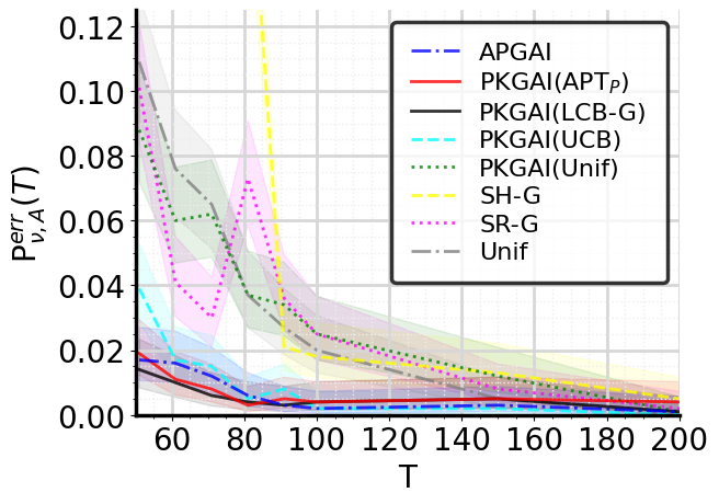
Figure 1: Fixed-budget empirical error on our outcome scoring application (see RealL in Table 3).

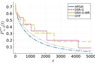
Figure 2: Anytime empirical error on Gaussian instances (a) $\mu\in\{0.55,0.45\}^{10}$ where $|\mathcal{A}_{\theta}|=3$ for $\theta=0.5$ and (b) $\mu=-(0.1,0.4,0.5,0.6)$ for $\theta=0$.

Fixed-budget Empirical Error

The APGAI algorithm is compared to fixed-budget GAI algorithms: SR-G, SH-G, PKGAI and Unif. For a fair comparison, the threshold functions in PKGAI do not use prior knowledge (see Appendix I.2.2, where theoretical thresholds are also considered). Several index policies are considered for PKGAI: Unif, APT_P, UCB and LCB-G. At time $t$, the latter selects among the set $\mathcal{S}_{t}$ of active candidates $a_{t}\leftarrow\arg\,\max_{a\in\mathcal{S}_{t}}\sqrt{N_{a}(t)}\text{LCB}(a,t)$, where LCB$(a,t)$ is the lower confidence bound on $\mu_{a}-\theta$ at time $t$. For a budget $T$ up to $200$, our results are averaged over $1,000$ runs, and confidence intervals are displayed. On our outcome scoring application, Figure 1 first shows that all uniform samplings (SH-G, SR-G, Unif and PKGAI(Unif)) are less efficient at detecting one of the good arms contrary to the adaptive strategies. Moreover, APGAI actually performs as well as the elimination-based algorithms PKGAI($\star$), while allowing early stopping as well. In Appendix I.3, we confirm the good performance of APGAI in terms of fixed-budget empirical error on other instances.

Anytime Empirical Error

The APGAI algorithm is compared to anytime GAI algorithms: DSR-G, DSH-G (see Section 3.1.1) and Unif. Since DSH-G has poor empirical performance (see Figure 4), we consider the heuristic DSH-G-WR where each SH instance keeps its history instead of discarding it. On two Gaussian instances ($\mathcal{A}_{\theta}(\mu)\neq\emptyset$ and $\mathcal{A}_{\theta}(\mu)=\emptyset$), Figure 2 shows that APGAI has significantly smaller empirical error compared to Unif, which is itself better than DSR-G and DSH-G-WR. Our results are averaged over $10,000$ runs, and confidence intervals are displayed. In Appendix I.4, we confirm the good performance of APGAI in terms of anytime empirical error on other instances, e.g.  when $\mathcal{A}_{\theta}(\mu)\neq\emptyset$ (Figure 18) and when $|\mathcal{A}_{\theta}(\mu)|$ varies (Figure 16). Overall, APGAI appears to have better empirical performance than suggested by Theorem 1 when $\mathcal{A}_{\theta}(\mu)\neq\emptyset$.

Empirical Stopping Time

The APGAI algorithm is compared to fixed-confidence GAI algorithms using the GLR stopping rule (5) with threshold (6) and confidence $\delta=0.01$: Murphy Sampling (MS (Kaufmann et al.,, 2018)), HDoC, LUCB-G (Kano et al.,, 2019), Track-and-Stop for GAI (TaS (Garivier and Kaufmann,, 2016)) and Unif (see Appendix I.2.3). In Figure 3, we study the impact of the number of good arms by considering Gaussian instances with two groups of arms. Our results are averaged over $1,000$ runs, and the standard deviations are displayed. Figure 3 shows that the empirical performance of APGAI is invariant to varying $|\mathcal{A}_{\theta}|$, and comparable to the one of TaS. In comparison, the other algorithms have worse performance, and they suffer from increased $|\mathcal{A}_{\theta}|$ since they have an exploration bonus for each good arm. In contrast, APGAI is greedy enough to only focus its allocation to one of the good arms. While APGAI achieves the best performance when there is no good arm, it can suffer from large outliers when good arms have dissimilar means (Figure 22 in Appendix I.5). To circumvent this problem, it is enough to add forced exploration to APGAI (Table 11). While APGAI was designed for anytime GAI, it is remarkable that it also has theoretical guarantees in fixed-confidence GAI, and relatively small empirical stopping time.

Figure 3: Empirical stopping time ($\delta=0.01$) on Gaussian instances $\mu\in\{0.5,-0.5\}^{100}$ where $|\mathcal{A}_{\theta}|\in\{5k\}_{k\in[19]}$ for $\theta=0$.

6 PERSPECTIVES

We propose APGAI, the first anytime and parameter-free sampling strategy for GAI in stochastic bandits, which is independent of a budget $T$ or a confidence $\delta$. In addition to showing its good empirical performance, we also provided guarantees on its probability of error at any deterministic time $t$ (Theorem 1) and on its expected sample complexity at any confidence $\delta$ when combined with the GLR stopping time (5) (Theorem 2). As such, APGAI allows both continuation and early stopping. We reviewed and analyzed a large number of baselines for each GAI setting for comparison.

While we considered unstructured multi-armed bandits, many applications have a known structure. Investigating the GAI problem on e.g.  linear or infinitely-armed bandits, would be an interesting subsequent work. In particular, working in a structured framework when facing a possibly infinite number of arms would bring out more compelling questions about how to explore the arm space in a both tractable and meaningful way.

Acknowledgements

Experiments presented in this paper were carried out using the Grid’5000 testbed, supported by a scientific interest group hosted by Inria and including CNRS, RENATER and several Universities as well as other organizations (see https://www.grid5000.fr). This work has been partially supported by the THIA ANR program “AI_PhD@Lille”.

Checklist

1. For all models and algorithms presented, check if you include:

   1. A clear description of the mathematical setting, assumptions, algorithm, and/or model. Yes, in Sections 1 and 2.

   2. An analysis of the properties and complexity (time, space, sample size) of any algorithm. Yes, in Sections 2 and 3.

   3. (Optional) Anonymized source code, with specification of all dependencies, including external libraries. Yes, in the supplementary materials as a zip folder.

2. For any theoretical claim, check if you include:

   1. Statements of the full set of assumptions of all theoretical results. Yes, in Sections 3 and 4.

   2. Complete proofs of all theoretical results. Yes, in Appendices B, C, D and F.

   3. Clear explanations of any assumptions. Yes, in Section 1.

3. For all figures and tables that present empirical results, check if you include:

   1. The code, data, and instructions needed to reproduce the main experimental results (either in the supplemental material or as a URL). Yes, in supplementary and Appendix I.2.

   2. All the training details (e.g., data splits, hyperparameters, how they were chosen). Yes, in Appendices I.1 and I.2.

   3. A clear definition of the specific measure or statistics and error bars (e.g., with respect to the random seed after running experiments multiple times). Yes, in Section 5.

   4. A description of the computing infrastructure used. (e.g., type of GPUs, internal cluster, or cloud provider). Yes, in Appendix I.2.

4. If you are using existing assets (e.g., code, data, models) or curating/releasing new assets, check if you include:

   1. Citations of the creator If your work uses existing assets. Not Applicable.

   2. The license information of the assets, if applicable. Yes, in supplementary.

   3. New assets either in the supplemental material or as a URL, if applicable. Yes, in supplementary.

   4. Information about consent from data providers/curators. Yes, in supplementary.

   5. Discussion of sensible content if applicable, e.g., personally identifiable information or offensive content. Not Applicable.

5. If you used crowdsourcing or conducted research with human subjects, check if you include:

   1. The full text of instructions given to participants and screenshots. Not Applicable.

   2. Descriptions of potential participant risks, with links to Institutional Review Board (IRB) approvals if applicable. Not Applicable.

   3. The estimated hourly wage paid to participants and the total amount spent on participant compensation. Not Applicable.

Appendix A OUTLINE

The appendices are organized as follows:

• The anytime guarantees of proof APGAI on the probability of error (Theorem 1) are proven in Appendix B.

• Appendix C gathers error guarantees on other algorithms that are used as comparison with the anytime error guarantees of APGAI: UnifB (Theorem 4), SH-G (Theorem 5) and SR-G (Theorem 6).

• We propose the meta-algorithm PKGAI in Appendix D, and analyze its error guarantees for several choices of index policy (Theorems 7 and 8).

• Appendix E gives the proof of Lemma 1. Then, we link the ATP_P index and the GLR stopping rule (5) with the generalized likelihood ratio for GAI.

• The proof of Theorem 2 for APGAI when combined with the GLR stopping (5) using threshold (6) is detailed in Appendix F.

• Appendix G contains the proof of Lemma 2, and provides sequence of concentration events which are used for our proofs.

• Appendix H gathers existing and new technical results which are used for our proofs.

• In Appendix I, we provide more details on our experimental study, as well as additional experiments.

Appendix B ANALYSIS OF APGAI: THEOREM 1

The APGAI algorithm is independent of a budget $T$ or a confidence $\delta$ which would define a stopping condition. In the following, we consider the behavior of APGAI when it is sampling forever. Therefore, we provide guarantees at all time $T$, where $T$ can be seen as an analysis parameter. In order to upper bound the probability of the complementary of the concentration event at time $T$, we use an analytical parameter denoted by $\delta$ which will be inverted to obtain an upper bound on the probability of error. We emphasize that the $\delta$ used in Appendix B is not the same $\delta$ than the one to calibrate the stopping thresholds used in the GLR stopping (5). We recall that each arm is pulled $n_{0}$ times as initialization.

Proof Strategy

Let $\mu\in\mathbb{R}^{K}$ such that $\mu_{a}\neq\theta$ for all $a\in\mathcal{A}$. For all $T>n_{0}K$ and $\delta\in(0,1)$, let $\tilde{\mathcal{E}}_{T,\delta}$ as in (22) for $s=0$, i.e.

$$\tilde{\mathcal{E}}_{T,\delta}=\left\{\forall a\in\mathcal{A},\forall t\leq T,\>|\hat{\mu}_{a}(t)-\mu_{a}|<\sqrt{\frac{2\tilde{f}_{1}(T,\delta)}{N_{a}(t)}}\right\}\>,$$ (7)

$$\text{with}\quad\tilde{f}_{1}(T,\delta)=\frac{1}{2}\overline{W}_{-1}(2\log(1/\delta)+2\log(2+\log T)+2)\>,$$

Recall that the error event $\mathcal{E}^{\text{err}}_{\mu}(T)$ is defined as

$$\mathcal{E}^{\text{err}}_{\mu}(T):=\left\{\left(\mathcal{A}_{\theta}\neq\emptyset\cap(\hat{a}_{T}=\emptyset\cup\mu_{\hat{a}_{T}}<\theta)\right)\cup\left(\mathcal{A}_{\theta}=\emptyset\cap\hat{a}_{T}\neq\emptyset\right)\right\}\>.$$

Using Lemma 22, we have $\mathbb{P}_{\nu}(\tilde{\mathcal{E}}_{T,\delta}^{\complement})\leq K\delta$. Suppose that we have constructed a time $T_{\mu}(\delta)\geq n_{0}K$ such that $\tilde{\mathcal{E}}_{T,\delta}\subseteq\mathcal{E}^{\text{err}}_{\mu}(T)^{\complement}$ for $T>T_{\mu}(\delta)$. Then, we obtain

$$\forall T>T_{\mu}(\delta),\quad P^{\text{err}}_{\nu,\cdot}(T)=\mathbb{P}_{\nu}(\mathcal{E}^{\text{err}}_{\mu}(T))\leq K\delta\quad\text{hence}\quad P^{\text{err}}_{\nu,\cdot}(T)\leq K\inf\{\delta\mid\>T>T_{\mu}(\delta)\}\>,$$

where the last inequality is obtained by taking the infimum. To prove Theorem 1, we will distinguish between instances $\mu$ such that $\mathcal{A}_{\theta}=\emptyset$ (Appendix B.1) and instances $\mu$ such that $\mathcal{A}_{\theta}\neq\emptyset$ (Appendix B.2).

Lemma 3 is the key technical tool on which our proofs rely on. It assumes the existence of a sequence of “bad” events such that, under each “bad” event, the arm selected to be pulled next was not sampled a lot yet. Then, it shows that the number of times those “bad” events occur is small.

Lemma 3.

Let $\delta\in(0,1]$ and $T>n_{0}K$. Let $(A_{t}(T,\delta))_{T\geq t\geq n_{0}K}$ be a sequence of events and $(D_{a}(T,\delta))_{a\in\mathcal{A}}$ be positive thresholds satisfying that, for all $t\in(n_{0}K,T]\cap\mathbb{N}$, under the event $A_{t}(T,\delta)$,

$$N_{a_{t+1}}(t)\leq D_{a_{t+1}}(T,\delta)\quad\text{and}\quad N_{a_{t+1}}(t+1)=N_{a_{t+1}}(t)+1\>.$$

Then, we have $\sum_{t=n_{0}K+1}^{T}\mathds{1}\left(A_{t}(T,\delta)\right)\leq\sum_{a\in\mathcal{A}}D_{a}(T,\delta)$.

Proof.

Using the inclusion of events given by the assumption on $(A_{t}(T,\delta))_{T\geq t>K}$, we obtain

$$\sum_{t=n_{0}K+1}^{T}\mathds{1}\left(A_{t}(T,\delta)\right) \leq\sum_{t=n_{0}K+1}^{T}\mathds{1}\left(N_{a_{t+1}}(t)\leq D_{a_{t+1}}(T,\delta),\>N_{a_{t+1}}(t+1)=N_{a_{t+1}}(t)+1\right)$$

$$\leq\sum_{a\in\mathcal{A}}\sum_{t=n_{0}K+1}^{T}\mathds{1}\left(N_{a}(t)\leq D_{a}(T,\delta),\>N_{a}(t+1)=N_{a}(t)+1\right)\leq\sum_{a\in\mathcal{A}}D_{a}(T,\delta)\>.$$

The second inequality is obtained by union bound. The third inequality is direct since the number of times one can increment by one a quantity that is positive and bounded by $D_{a}(T,\delta)$ is at most $D_{a}(T,\delta)$. ∎

In our proofs, we derive necessary conditions for a mistake to be made and show that having those conditions that hold is a “bad” event satisfying the condition of Lemma 3. Theorem 1 is obtained by combining Lemmas 4 and 8.

B.1 Instances Where $\mathcal{A}_{\theta}=\emptyset$

When $\mathcal{A}_{\theta}=\emptyset$, we have $\mathcal{E}^{\text{err}}_{\mu}(T)=\{\hat{a}_{T}\neq\emptyset\}$. Lemma 4 gives an upper bound on the probability of error based on the recommendation of the APGAI algorithm holding for all time $T$.

Lemma 4.

Let $p(x)=\sqrt{x}\exp(-x)$. For all $\mu\in\mathbb{R}^{K}$ such that $\max_{a\in\mathcal{A}}\mu_{a}<\theta$, the APGAI satisfies, for all $T>n_{0}K$ such that it has not stopped sampling at time $T$,

$$\mathbb{P}_{\nu}(\hat{a}_{T}\neq\emptyset)\leq Ke\sqrt{2}(2+\log T)p\left(\frac{T-n_{0}K}{18H_{1}(\mu)}\right)\>.$$

Proof.

In order to prove Lemma 4, we show key intermediate properties of the APGAI algorithm when $\mathcal{A}_{\theta}=\emptyset$.

Error Due to Undersampled Arms

At a fixed $(T,\delta)$, we define the set of undersampled arms as

$$\forall t\in(n_{0}K,T]\cap\mathbb{N},\quad U_{t}(T,\delta)=\left\{a\in\mathcal{A}\mid N_{a}(t)\leq\frac{2\tilde{f}_{1}(T,\delta)}{\Delta_{a}^{2}}\right\}\>.$$

We show that a necessary condition for an error to occur at time $t$, i.e.  $\hat{a}_{t}\neq\emptyset$, is that there exists undersampled arms, i.e.  $U_{t}(T,\delta)\neq\emptyset$ (Lemma 5).

Lemma 5.

For all $T\in\mathbb{N}$, under the event $\tilde{\mathcal{E}}_{T,\delta}$ as in (7), for all $t\in(n_{0}K,T]\cap\mathbb{N}$, we have

$$\hat{a}_{t}\neq\emptyset\quad\implies\quad U_{t}(T,\delta)\neq\emptyset\>.$$

Proof.

Not recommending $\emptyset$ only happens when the largest empirical mean exceeds $\theta$, i.e.  $\max_{a\in\mathcal{A}}\hat{\mu}_{a}(t)>\theta$. Let $\hat{a}_{t}=\arg\,\max_{a\in\mathcal{A}}W^{+}_{a}(t)$ which satisfies $\hat{\mu}_{\hat{a}_{t}}(t)>\theta$. Under $\tilde{\mathcal{E}}_{T,\delta}$ as in (7), we have

$$\theta<\hat{\mu}_{\hat{a}_{t}}(t)\leq\mu_{\hat{a}_{t}}+\sqrt{\frac{2\tilde{f}_{1}(T,\delta)}{N_{\hat{a}_{t}}(t)}}\quad\text{hence}\quad\hat{a}_{t}\in U_{t}(T,\delta)\>.$$

∎

No Remaining Undersampled Arms

We show that the events $\{U_{t}(T,\delta)\neq\emptyset\}$ satisfy the conditions of Lemma 3 (Lemma 6). In other words, if there are still undersampled arms at time $t$, then $a_{t+1}$ has not been sampled too many times.

Lemma 6.

Let $\delta\in(0,1)$ and $T>n_{0}K$. Under event $\tilde{\mathcal{E}}_{T,\delta}$, for all $t\in(n_{0}K,T]\cap\mathbb{N}$ such that $U_{t}(T,\delta)\neq\emptyset$, we have

$$N_{a_{t+1}}(t)\leq\frac{18\tilde{f}_{1}(T,\delta)}{\Delta_{a_{t+1}}^{2}}\quad\text{and}\quad N_{a_{t+1}}(t+1)=N_{a_{t+1}}(t)+1\>.$$

Proof.

We will be interested in three distinct cases since

$$\{U_{t}(T,\delta)=\emptyset\} = \underbrace{\{U_{t}(T,\delta)=\emptyset,\>\max_{a\in\mathcal{A}}\hat{\mu}_{a}(t)>\theta\}}_{\text{Case 1}}\cup\underbrace{\{U_{t}(T,\delta)=\emptyset,\>\max_{a\in\mathcal{A}}\hat{\mu}_{a}(t)<\theta\}}_{\text{Case 2}}$$

$$\quad\cup\underbrace{\{U_{t}(T,\delta)=\emptyset,\>\max_{a\in\mathcal{A}}\hat{\mu}_{a}(t)=\theta\}}_{\text{Case 3}}$$

Case 1. Let $t\in(n_{0}K,T]\cap\mathbb{N}$ such that $U_{t}(T,\delta)\neq\emptyset$ and $\max_{a\in\mathcal{A}}\hat{\mu}_{a}(t)>\theta$. Let $c=\arg\,\max_{a\in\mathcal{A}}\hat{\mu}_{a}(t)$. Since $W^{+}_{c}(t)>0$ and $a_{t+1}\in\arg\,\max_{a\in\mathcal{A}}W_{a}^{+}(t)$, we obtain $\hat{\mu}_{a_{t+1}}(t)>\theta$. Then, under $\tilde{\mathcal{E}}_{T,\delta}$ as in (7), we have

$$\sqrt{N_{a_{t+1}}(t)}(\hat{\mu}_{a_{t+1}}(t)-\theta)_{+} =\sqrt{N_{a_{t+1}}(t)}(\hat{\mu}_{a_{t+1}}(t)-\theta)\leq\sqrt{N_{a_{t+1}}(t)}(\mu_{a_{t+1}}-\theta)+\sqrt{2\tilde{f}_{1}(T,\delta)}\>.$$

Using that $W_{a_{t+1}}^{+}(t)>0$, we obtain

$$N_{a_{t+1}}(t)\leq\frac{2\tilde{f}_{1}(T,\delta)}{\Delta_{a_{t+1}}^{2}}\quad\text{and}\quad N_{a_{t+1}}(t+1)=N_{a_{t+1}}(t)+1\>.$$

Case 2. Let $t\in(n_{0}K,T]\cap\mathbb{N}$ such that $U_{t}(T,\delta)\neq\emptyset$ and $\max_{a\in\mathcal{A}}\hat{\mu}_{a}(t)<\theta$. Let $a_{t+1}\in\arg\,\min_{a\in\mathcal{A}}W_{a}^{-}(t)$ and $a\in U_{t}(T,\delta)$. Then, under $\tilde{\mathcal{E}}_{T,\delta}$ as in (7), we have

$$\sqrt{N_{a_{t+1}}(t)}(\theta-\mu_{a_{t+1}})-\sqrt{2\tilde{f}_{1}(T,\delta)}\leq\sqrt{N_{a_{t+1}}(t)}(\theta-\hat{\mu}_{a_{t+1}}(t))=\sqrt{N_{a_{t+1}}(t)}(\theta-\hat{\mu}_{a_{t+1}}(t))_{+}\>,$$

$$\sqrt{N_{a}(t)}(\theta-\hat{\mu}_{a}(t))_{+}=\sqrt{N_{a}(t)}(\theta-\hat{\mu}_{a}(t))\leq\sqrt{N_{a}(t)}(\theta-\mu_{a})+\sqrt{2\tilde{f}_{1}(T,\delta)}\leq 2\sqrt{2\tilde{f}_{1}(T,\delta)}\>.$$

Using that $W_{a_{t+1}}^{-}(t)\leq W_{a}^{-}(t)$, we have proven that

$$N_{a_{t+1}}(t)\leq\frac{18\tilde{f}_{1}(T,\delta)}{\Delta_{a_{t+1}}^{2}}\quad\text{and}\quad N_{a_{t+1}}(t+1)=N_{a_{t+1}}(t)+1\>.$$

Case 3. Let $t\in(n_{0}K,T]\cap\mathbb{N}$ such that $U_{t}(T,\delta)\neq\emptyset$ and $\max_{a\in\mathcal{A}}\hat{\mu}_{a}(t)=\theta$. Then, $\arg\,\min_{a\in\mathcal{A}}W_{a}^{-}(t)=\{a\in\mathcal{A}\mid\hat{\mu}_{a}(t)=\theta\}$. Therefore, we have $\hat{\mu}_{a_{t+1}}(t)=\theta$ hence

$$\theta=\hat{\mu}_{a_{t+1}}(t)\leq\mu_{a_{t+1}}+\sqrt{\frac{2\tilde{f}_{1}(T,\delta)}{N_{a_{t+1}}(t)}}\>.$$

Therefore, we have proven that

$$N_{a_{t+1}}(t)\leq\frac{2\tilde{f}_{1}(T,\delta)}{\Delta_{a_{t+1}}^{2}}\quad\text{and}\quad N_{a_{t+1}}(t+1)=N_{a_{t+1}}(t)+1\>.$$

Summary. Combing the three above cases yields the result. ∎

Lemma 7 provides a time after which all arms are sampled enough, hence no error will be made.

Lemma 7.

Let us define

$$T_{\mu}(\delta)=\sup\left\{T\mid T\leq 18H_{1}(\mu)\tilde{f}_{1}(T,\delta)+n_{0}K\right\}\>.$$

For all $T>T_{\mu}(\delta)$, under the event $\tilde{\mathcal{E}}_{T,\delta}$ as in (7), we have $U_{T}(T,\delta)=\emptyset$.

Proof.

Combining Lemmas 6 and 3, we obtain

$$\sum_{t=n_{0}K+1}^{T}\mathds{1}\left(U_{t}(T,\delta)\neq\emptyset\right) \leq 18H_{1}(\mu)\tilde{f}_{1}(T,\delta)\>.$$

For all $a\in\mathcal{A}$, let us define $t_{a}(T,\delta)=\max\{t\in(n_{0}K,T]\cap\mathbb{N}\mid a\in U_{t}(T,\delta)\}$. By definition, we have $a\in U_{t}(T,\delta)$ for all $t\in(n_{0}K,t_{a}(T,\delta)]$ and $a\notin U_{t}(T,\delta)$ for all $t\in(t_{a}(T,\delta),T]$. Therefore, for all $t\in(n_{0}K,\max_{a\in\mathcal{A}}t_{a}(T,\delta)]$, we have $U_{t}(T,\delta)\neq\emptyset$ and $U_{t}(T,\delta)=\emptyset$ for all $t>\max_{a\in\mathcal{A}}t_{a}(T,\delta)$, hence

$$\max_{a\in\mathcal{A}}(t_{a}(T,\delta)-n_{0}K)=\sum_{t=n_{0}K+1}^{T}\mathds{1}\left(U_{t}(T,\delta)\neq\emptyset\right)\leq 18H_{1}(\mu)\tilde{f}_{1}(T,\delta)\>.$$

Let $T_{\mu}(\delta)$ defined as in the statement of Lemma 7 and $T>T_{\mu}(\delta)$. Then, we have

$$T-n_{0}K>18H_{1}(\mu)\tilde{f}_{1}(T,\delta)\geq\max_{a\in\mathcal{A}}(t_{a}(T,\delta)-n_{0}K)\>,$$

hence $T>\max_{a\in\mathcal{A}}t_{a}(T,\delta)$. This concludes the proof that $U_{T}(T,\delta)=\emptyset$. ∎

Conclusion

Let $T_{\mu}(\delta)$ as in Lemma 7. Combining Lemmas 7,  5 and 22, we obtain

$$\mathbb{P}_{\nu}(\hat{a}_{T}\neq\emptyset) \leq K\inf\{\delta\mid\>T>T_{\mu}(\delta)\}\leq Ke\sqrt{2}(2+\log T)\sqrt{\frac{T-n_{0}K}{18H_{1}(\mu)}}\exp\left(-\frac{T-n_{0}K}{18H_{1}(\mu)}\right)\>,$$

where the last inequality uses Lemma 26. This concludes the proof of Lemma 4. ∎

B.2 Instances Where $\mathcal{A}_{\theta}\neq\emptyset$

When $\mathcal{A}_{\theta}=\emptyset$, we have $\mathcal{E}^{\text{err}}_{\mu}(T)=\{\hat{a}_{T}=\emptyset\}\cup\{\hat{a}_{T}\in\mathcal{A}_{\theta}^{\complement}\}$. Lemma 8 gives an upper bound on the probability of error based on the recommendation of APGAI holding for all time $T$.

Lemma 8.

Let $p(x)=\sqrt{x}\exp(-x)$. For all $\mu\in\mathbb{R}^{K}$ such that $\mathcal{A}_{\theta}\neq\emptyset$ and $\mu_{a}\neq\theta$ for all $a\in\mathcal{A}$, the APGAI satisfies, for all $T>n_{0}K$ such that it has not stopped sampling at time $T$,

$$\mathbb{P}\left(\{\hat{a}_{T}=\emptyset\}\cup\{\hat{a}_{T}\in\mathcal{A}_{\theta}^{\complement}\}\right) \leq Ke\sqrt{2}(2+\log T)p\left(\frac{T-n_{0}K-2|\mathcal{A}_{\theta}|}{4H_{1}(\mu)}\right)\>.$$

Proof.

In order to prove Lemma 8, we show key intermediate properties of the APGAI algorithm when $\mathcal{A}_{\theta}\neq\emptyset$.

Error Due to Undersampled Arms

At a fixed $(T,\delta)$, we define the set of under-sampled arms as

$$\forall t\in(n_{0}K,T]\cap\mathbb{N},\quad U_{t}(T,\delta) =\left\{a\in\mathcal{A}\mid N_{a}(t)\leq\left(\sqrt{\frac{2\tilde{f}_{1}(T,\delta)}{\Delta_{a}^{2}}}+1\right)^{2}\right\}\>.$$

Lemma 9 shows that a necessary condition to recommend $\emptyset$ at time $t$ is that all the good arms are undersampled arms, i.e.  $\mathcal{A}_{\theta}\subseteq U_{t}(T,\delta)$. It also shows that a necessary condition to recommend $\hat{a}_{t}\in\mathcal{A}_{\theta}^{\complement}$ at time $t$ is that this arm is undersampled and will be sampled next, i.e.  $\hat{a}_{t}=a_{t+1}\in\mathcal{A}_{\theta}^{\complement}\cap U_{t}(T,\delta)$.

Lemma 9.

For all $T\in\mathbb{N}$, under the event $\tilde{\mathcal{E}}_{T,\delta}$ as in (7), for all $t\in(n_{0}K,T]\cap\mathbb{N}$, we have

$$\hat{a}_{t}=\emptyset\quad\implies\quad\mathcal{A}_{\theta}\subseteq U_{t}(T,\delta)\>,$$

$$\hat{a}_{t}\in\mathcal{A}_{\theta}^{\complement}\quad\implies\quad\hat{a}_{t}=a_{t+1}\in\mathcal{A}_{\theta}^{\complement}\cap U_{t}(T,\delta)\>.$$

Proof.

Case 1. Suppose that $\hat{a}_{t}=\emptyset$, hence $\max\hat{\mu}_{a}(t)\leq\theta$. Then, for all $a\in\mathcal{A}_{\theta}$, we have

$$\theta\geq\hat{\mu}_{a}(t)\geq\mu_{a}-\sqrt{\frac{2f_{1}(T,\delta)}{N_{a}(t)}}\>,$$

hence $\mathcal{A}_{\theta}\subseteq U_{t}(T,\delta)$.

Case 2. Suppose that $\hat{a}_{t}\notin\mathcal{A}_{\theta}$, hence $\max\hat{\mu}_{a}(t)>\theta$. Since $\hat{a}_{t}=a_{t+1}\in\arg\,\max_{a\in\mathcal{A}}W^{+}_{a}(t)$, we have $\hat{\mu}_{\hat{a}_{t}}(t)>\theta$. Then, we have

$$\theta<\hat{\mu}_{a_{t+1}}(t)\leq\mu_{a_{t+1}}+\sqrt{\frac{2f_{1}(T,\delta)}{N_{a_{t+1}}(t)}}\>,$$

hence $a_{t+1}\in\mathcal{A}_{\theta}^{\complement}\cap U_{t}(T,\delta)$. ∎

One Good Arm Not Undersampled

Lemma 10 shows that the events $\{\mathcal{A}_{\theta}\subseteq U_{t}(T,\delta)\}$ are satisfying the conditions of Lemma 3. In other words, having all the good arms undersampled implies that the next arm we will pull was not sampled a lot.

Lemma 10.

Let $\delta\in(0,1)$ and $T>n_{0}K$. Under event $\tilde{\mathcal{E}}_{T,\delta}$, for all $t\in(n_{0}K,T]\cap\mathbb{N}$ such that $\mathcal{A}_{\theta}\subseteq U_{t}(T,\delta)$, we have

$$N_{a_{t+1}}(t)\leq D_{a_{t+1}}(T,\delta)\quad\text{and}\quad N_{a_{t+1}}(t+1)=N_{a_{t+1}}(t)+1\>,$$

where $D_{a}(T,\delta)=\left(\Delta_{a}^{-1}\sqrt{2\tilde{f}_{1}(T,\delta)}+1\right)^{2}$ for all $a\in\mathcal{A}_{\theta}$ and $D_{a}(T,\delta)=2\tilde{f}_{1}(T,\delta)\Delta_{a}^{-2}$ for all $a\notin\mathcal{A}_{\theta}$.

Proof.

Let $t\in(n_{0}K,T]\cap\mathbb{N}$ such that $\mathcal{A}_{\theta}\subseteq U_{t}(T,\delta)$. When $a_{t+1}\in\mathcal{A}_{\theta}$, we have directly that

$$N_{a_{t+1}}(t)\leq\left(\sqrt{\frac{2\tilde{f}_{1}(T,\delta)}{\Delta_{a_{t+1}}^{2}}}+1\right)^{2}\quad\text{and}\quad N_{a_{t+1}}(t+1)=N_{a_{t+1}}(t)+1\>.$$

In the following, we consider $a_{t+1}\notin\mathcal{A}_{\theta}$.

We will be interested in three cases since

$$\{\mathcal{A}_{\theta}\subseteq U_{t}(T,\delta),\>a_{t+1}\notin\mathcal{A}_{\theta}\} = \underbrace{\{\mathcal{A}_{\theta}\subseteq U_{t}(T,\delta),\>a_{t+1}\notin\mathcal{A}_{\theta},\>\max_{a\in\mathcal{A}}\hat{\mu}_{a}(t)>\theta\}}_{\text{Case 1}}$$

$$\cup\underbrace{\{\mathcal{A}_{\theta}\subseteq U_{t}(T,\delta),\>a_{t+1}\notin\mathcal{A}_{\theta},\>\max_{a\in\mathcal{A}}\hat{\mu}_{a}(t)<\theta\}}_{\text{Case 2}}\quad\cup\underbrace{\{\mathcal{A}_{\theta}\subseteq U_{t}(T,\delta),\>a_{t+1}\notin\mathcal{A}_{\theta},\>\max_{a\in\mathcal{A}}\hat{\mu}_{a}(t)=\theta\}}_{\text{Case 3}}\>.$$

Case 1. Let $t\in(n_{0}K,T]\cap\mathbb{N}$ such that $\mathcal{A}_{\theta}\subseteq U_{t}(T,\delta)$, $a_{t+1}\notin\mathcal{A}_{\theta}$ and $\max_{a\in\mathcal{A}}\hat{\mu}_{a}(t)>\theta$. Let $c=\arg\,\max_{a\in\mathcal{A}}\hat{\mu}_{a}(t)$. Since $W^{+}_{c}(t)>0$ and $a_{t+1}\in\arg\,\max_{a\in\mathcal{A}}W_{a}^{+}(t)$, we have $\hat{\mu}_{a_{t+1}}(t)>\theta$. Since $a_{t+1}\notin\mathcal{A}_{\theta}$, under $\tilde{\mathcal{E}}_{T,\delta}$ as in (7), we have

$$\sqrt{N_{a_{t+1}}(t)}(\hat{\mu}_{a_{t+1}}(t)-\theta)_{+}=\sqrt{N_{a_{t+1}}(t)}(\hat{\mu}_{a_{t+1}}(t)-\theta)\leq\sqrt{N_{a_{t+1}}(t)}(\mu_{a_{t+1}}-\theta)+\sqrt{2\tilde{f}_{1}(T,\delta)}\>.$$

Using that $W_{a_{t+1}}^{+}(t)>0$, we obtain

$$N_{a_{t+1}}(t)\leq\frac{2\tilde{f}_{1}(T,\delta)}{\Delta_{a_{t+1}}^{2}}\quad\text{and}\quad N_{a_{t+1}}(t+1)=N_{a_{t+1}}(t)+1\>.$$

Case 2. Let $t\in(n_{0}K,T]\cap\mathbb{N}$ such that $\mathcal{A}_{\theta}\subseteq U_{t}(T,\delta)$, $a_{t+1}\notin\mathcal{A}_{\theta}$ and $\max_{a\in\mathcal{A}}\hat{\mu}_{a}(t)<\theta$. Let $a_{t+1}\in\arg\,\min_{a\in\mathcal{A}}W_{a}^{-}(t)$. Since $a_{t+1}\notin\mathcal{A}_{\theta}$, under $\tilde{\mathcal{E}}_{T,\delta}$ as in (7), for all $a\in\mathcal{A}_{\theta}$, we have

$$\sqrt{N_{a_{t+1}}(t)}(\theta-\mu_{a_{t+1}})-\sqrt{2\tilde{f}_{1}(T,\delta)}\leq\sqrt{N_{a_{t+1}}(t)}(\theta-\hat{\mu}_{a_{t+1}}(t))=\sqrt{N_{a_{t+1}}(t)}(\theta-\hat{\mu}_{a_{t+1}}(t))_{+}$$

$$\sqrt{N_{a}(t)}(\theta-\hat{\mu}_{a}(t))_{+}=\sqrt{N_{a}(t)}(\theta-\hat{\mu}_{a}(t))\leq\sqrt{N_{a}(t)}(\theta-\mu_{a})+\sqrt{2\tilde{f}_{1}(T,\delta)}\leq\sqrt{2\tilde{f}_{1}(T,\delta)}\>.$$

Combining both inequality by using that $W_{a_{t+1}}^{-}(t)\leq W_{a}^{-}(t)$ yields $\sqrt{N_{a_{t+1}}(t)}(\theta-\mu_{a_{t+1}})\leq 2\sqrt{2\tilde{f}_{1}(T,\delta)}$, hence

$$N_{a_{t+1}}(t)\leq\frac{8\tilde{f}_{1}(T,\delta)}{\Delta_{a_{t+1}}^{2}}\quad\text{and}\quad N_{a_{t+1}}(t+1)=N_{a_{t+1}}(t)+1\>.$$

Case 3. Let $t\in(n_{0}K,T]\cap\mathbb{N}$ such that $\mathcal{A}_{\theta}\subseteq U_{t}(T,\delta)$, $a_{t+1}\notin\mathcal{A}_{\theta}$ and $\max_{a\in\mathcal{A}}\hat{\mu}_{a}(t)=\theta$. Then, $a_{t+1}\in\arg\,\min_{a\in\mathcal{A}}W_{a}^{-}(t)=\{a\in\mathcal{A}\mid\hat{\mu}_{a}(t)=\theta\}$. Therefore, we have

$$\theta=\hat{\mu}_{a_{t+1}}(t)\leq\mu_{a_{t+1}}+\sqrt{\frac{2\tilde{f}_{1}(T,\delta)}{N_{a_{t+1}}(t)}}\>.$$

Since $a_{t+1}\notin\mathcal{A}_{\theta}$, we obtain

$$N_{a_{t+1}}(t)\leq\frac{2\tilde{f}_{1}(T,\delta)}{\Delta_{a_{t+1}}^{2}}\quad\text{and}\quad N_{a_{t+1}}(t+1)=N_{a_{t+1}}(t)+1\>.$$

Summary. Combing the three above cases yields the result. ∎

Lemma 11 shows that having a good arm that is sampled enough, i.e.  $\mathcal{A}_{\theta}\cap U_{t}(T,\delta)^{\complement}\neq\emptyset$, is a sufficient condition to recommend a good arm, i.e.  $\hat{a}_{t}\in\mathcal{A}_{\theta}$.

Lemma 11.

Let $\delta\in(0,1)$ and $T>n_{0}K$. Under event $\tilde{\mathcal{E}}_{T,\delta}$, for all $t\in(n_{0}K,T]\cap\mathbb{N}$ such that $\mathcal{A}_{\theta}\cap U_{t}(T,\delta)^{\complement}\neq\emptyset$, we have $\hat{a}_{t}\in\mathcal{A}_{\theta}$.

Proof.

Let $t\in(n_{0}K,T]\cap\mathbb{N}$ such that $\mathcal{A}_{\theta}\cap U_{t}(T,\delta)^{\complement}\neq\emptyset$. Let $a\in\mathcal{A}_{\theta}\cap U_{t}(T,\delta)^{\complement}$, hence we have

$$N_{a}(t)>\left(\sqrt{\frac{2\tilde{f}_{1}(T,\delta)}{(\mu_{a}-\theta)^{2}}}+1\right)^{2}>\frac{2\tilde{f}_{1}(T,\delta)}{(\mu_{a}-\theta)^{2}}\>.$$ (8)

Therefore, under $\tilde{\mathcal{E}}_{T,\delta}$ as in (7), we have

$$\max_{b\in\mathcal{A}}\hat{\mu}_{b}(t)\geq\hat{\mu}_{a}(t)\geq\mu_{a}-\sqrt{\frac{2\tilde{f}_{1}(T,\delta)}{N_{a}(t)}}>\theta\>,$$

hence $\hat{a}_{t}=a_{t+1}\in\arg\,\max_{a\in\mathcal{A}}W_{a}^{+}(t)$.

Suppose towards contradiction that $\mathcal{A}_{\theta}^{\complement}\cap\arg\,\max_{a\in\mathcal{A}}W_{a}^{+}(t)\neq\emptyset$. Let $a\in\mathcal{A}_{\theta}^{\complement}\cap\arg\,\max_{a\in\mathcal{A}}W_{a}^{+}(t)\neq\emptyset$. It is direct to see that $\hat{\mu}_{a}(t)>\theta$, otherwise there is a contradiction. Then, using that $a\in\mathcal{A}_{\theta}^{\complement}$ (i.e.  $\mu_{a}\leq\theta$), we have for all $b\in\mathcal{A}_{\theta}\cap U_{t}(T,\delta)^{\complement}$

$$\sqrt{2\tilde{f}_{1}(T,\delta)}\geq\sqrt{N_{a}(t)}(\mu_{a}-\theta)+\sqrt{2\tilde{f}_{1}(T,\delta)}\geq\sqrt{N_{a}(t)}(\hat{\mu}_{a}(t)-\theta)=\sqrt{N_{a}(t)}(\hat{\mu}_{a}(t)-\theta)_{+}\>,$$

$$\sqrt{N_{b}(t)}(\hat{\mu}_{b}(t)-\theta)_{+}=\sqrt{N_{b}(t)}(\hat{\mu}_{b}(t)-\theta)\geq\sqrt{N_{b}(t)}(\mu_{b}-\theta)-\sqrt{\frac{2\tilde{f}_{1}(T,\delta)}{N_{b}(t)}}$$

$$\qquad>\left(\sqrt{N_{b}(t)}-1\right)(\mu_{b}-\theta)>\sqrt{2\tilde{f}_{1}(T,\delta)}\>,$$

where the two last inequalities are obtained by using (8) first the smaller thresholds, then the one in-between. Since $a\neq b$ and $W_{a}^{+}(t)\geq W_{b}^{+}(t)$, combining the above yields $\sqrt{2\tilde{f}_{1}(T,\delta)}>\sqrt{2\tilde{f}_{1}(T,\delta)}$ which is a contradiction. Therefore, we have proven that

$$\mathcal{A}_{\theta}\cap U_{t}(T,\delta)^{\complement}\neq\emptyset\quad \implies\quad\hat{a}_{t}\in\arg\,\max_{a\in\mathcal{A}}W_{a}^{+}(t)\>\land\>\mathcal{A}_{\theta}^{\complement}\cap\arg\,\max_{a\in\mathcal{A}}W_{a}^{+}(t)=\emptyset$$

$$\implies\quad\hat{a}_{t}\in\mathcal{A}_{\theta}\>.$$

∎

Lemma 12 provides a time after which there exists a good arms which is sampled enough, hence no error will be made.

Lemma 12.

Let us define

$$S_{\mu}(\delta)=\sup\left\{T\mid T\leq 4H_{1}(\mu)\tilde{f}_{1}(T,\delta)+n_{0}K+2|\mathcal{A}_{\theta}|\right\}\>.$$

For all $T>S_{\mu}(\delta)$, under the event $\tilde{\mathcal{E}}_{T,\delta}$ as in (7), we have $\mathcal{A}_{\theta}\cap U_{T}(T,\delta)^{\complement}\neq\emptyset$ and $\hat{a}_{t}\in\mathcal{A}_{\theta}$.

Proof.

Let $(D_{a}(T,\delta))_{a\in\mathcal{A}}$ as in Lemma 10. Combining Lemmas 10 and 3, we obtain

$$\sum_{t=n_{0}K+1}^{T}\mathds{1}\left(\mathcal{A}_{\theta}\subseteq U_{t}(T,\delta)\right) \leq\sum_{a\in\mathcal{A}}D_{a}(T,\delta)\>.$$

For all $a\in\mathcal{A}_{\theta}$, let us define $t_{a}(T,\delta)=\max\{t\in(n_{0}K,T]\cap\mathbb{N}\mid a\in U_{t}(T,\delta)\}$. By definition, we have $a\in U_{t}(T,\delta)$ for all $t\in(n_{0}K,t_{a}(T,\delta)]$ and $a\notin U_{t}(T,\delta)$ for all $t\in(t_{a}(T,\delta),T]$. Therefore, for all $t\in(n_{0}K,\min_{a\in\mathcal{A}_{\theta}}t_{a}(T,\delta)]$, we have $\mathcal{A}_{\theta}\subseteq U_{t}(T,\delta)$ and $\mathcal{A}_{\theta}\cap U_{t}(T,\delta)^{\complement}\neq\emptyset$ for all $t>\max_{a\in\mathcal{A}}t_{a}(T,\delta)$, hence

$$\min_{a\in\mathcal{A}_{\theta}}(t_{a}(T,\delta)-K)=\sum_{t=n_{0}K+1}^{T}\mathds{1}\left(\mathcal{A}_{\theta}\subseteq U_{t}(T,\delta)\right)\leq\sum_{a\in\mathcal{A}}D_{a}(T,\delta)\>.$$

Let $S_{\mu}(\delta)$ defined as in the statement of Lemma 12 and $T>S_{\mu}(\delta)$. Using that $(a+1)^{2}\leq 2a^{2}+2$, we have

$$S_{\mu}(\delta)\geq\sup\left\{T\mid T\leq\sum_{a\in\mathcal{A}}D_{a}(T,\delta)+n_{0}K\right\}\>.$$

Then, we have

$$T-n_{0}K>\sum_{a\in\mathcal{A}}D_{a}(T,\delta)\geq\min_{a\in\mathcal{A}_{\theta}}(t_{a}(T,\delta)-n_{0}K)\>,$$

hence $T>\min_{a\in\mathcal{A}_{\theta}}t_{a}(T,\delta)$. Therefore, we have $\mathcal{A}_{\theta}\cap U_{T}(T,\delta)^{\complement}\neq\emptyset$. Using Lemma 11, we obtain that $\hat{a}_{t}\in\mathcal{A}_{\theta}$. This concludes the proof. ∎

Conclusion

Let $S_{\mu}(\delta)$ as in Lemma 12. Combining Lemmas 12, 9 and 22, we obtain

$$\mathbb{P}_{\nu}(\{\hat{a}_{t}=\emptyset\}\cup\{\hat{a}_{t}\in\mathcal{A}_{\theta}^{\complement}\})\leq K\inf\{\delta\mid\>T>S_{\mu}(\delta)\}$$

$$\quad\leq Ke\sqrt{2}(2+\log T)\sqrt{\frac{T-n_{0}K-2|\mathcal{A}_{\theta}|}{4H_{1}(\mu)}}\exp\left(-\frac{T-n_{0}K-2|\mathcal{A}_{\theta}|}{4H_{1}(\mu)}\right)\>,$$

This concludes the proof. ∎

B.3 Unverifiable Sample Complexity

In Appendix B.3, we study the unverifiable sample complexity (Katz-Samuels and Jamieson,, 2020) (also discussed in Zhao et al., (2023)). This complexity is the minimum number of samples needed for an algorithm to output a correct answer with high probability. In particular, it does not require to check that the output is correct. Theorem 3 shows a deterministic upper bound on the unverifiable sample complexity of APGAI.

Theorem 3.

Let $\delta\in(0,1)$. The APGAI algorithm satisfies that, for any $1$-sub-Gaussian distribution with mean $\mu$ such that $\mu_{a}\neq\theta$ for all $a\in\mathcal{A}$,

$$\text{if }\mathcal{A}_{\theta}=\emptyset,\quad \mathbb{P}\left(\forall t>U_{\delta}(\mu),\>\hat{a}_{t}=\emptyset\right)\geq 1-\delta\>,$$

$$\text{if }\mathcal{A}_{\theta}\neq\emptyset,\quad \mathbb{P}\left(\forall t>U_{\delta}(\mu),\>\hat{a}_{t}\in\mathcal{A}_{\theta}\right)\geq 1-\delta\>.$$

The time $U_{\delta}(\mu)$ is the unverifiable sample complexity of APGAI for GAI defined as

$$U_{\delta}(\mu)=\begin{cases}h_{2}(\log(1/\delta),18H_{1}(\mu),n_{0}K)&\text{if }\mathcal{A}_{\theta}=\emptyset\;,\\ h_{2}(\log(1/\delta),4H_{1}(\mu),n_{0}K+2|\mathcal{A}_{\theta}|)&\text{otherwise }\;.\end{cases}$$ (9)

The function $h_{2}(\log(1/\delta),A,B):=A\overline{W}_{-1}(\log(1/\delta)+\frac{B}{A}+\log(A))$ satisfies that $h_{2}(\log(1/\delta),A,B)=_{\delta\to 0}A\log(1/\delta)+\mathcal{O}(\log\log(1/\delta))$.

Proof.

In Appendix B.1 and B.2, we consider the concentration event $\tilde{\mathcal{E}}_{T,\delta}$ that involved tighter concentration results with thresholds $\tilde{f}_{1}(T,\delta)$. Let $T>K$ and $\delta\in(0,1)$. It is direct to see that the same argument holds for the the concentration events $\mathcal{E}_{T,\delta}$ as in (20) for $s=0$, i.e.

$$\mathcal{E}_{T,\delta} =\left\{\forall a\in\mathcal{A},\forall t\leq T,\>|\hat{\mu}_{a}(t)-\mu_{a}|<\sqrt{\frac{2f_{1}(T,\delta)}{N_{a}(t)}}\right\}\>,$$

where $f_{1}(T,\delta)=\log(1/\delta)+\log T+\log K$. Using Lemma 21, we obtain that $\mathbb{P}_{\nu}(\mathcal{E}_{T,\delta})\leq\delta$.

Case 1: when $\mathcal{A}_{\theta}=\emptyset$. Let $T_{\mu}(\delta)$ defined similarly as in Lemma 7, i.e.

$$T_{\mu}(\delta):=\sup\left\{T\mid T\leq 18H_{1}(\mu)f_{1}(T,\delta)+n_{0}K\right\}\>.$$

To prove Theorem 1 when $\mathcal{A}_{\theta}=\emptyset$, we obtain as an intermediary result that: for all $T>T_{\mu}(\delta)$, $\{\hat{a}_{T}\neq\emptyset\}\subseteq\mathcal{E}_{T,\delta}^{\complement}$. Using a proof similar to Lemma 27, applying Lemma 25 yields that

$$T>T_{\mu}(\delta)\> \iff\>T>18H_{1}(\mu)\log T+18H_{1}(\mu)\log(1/\delta)+n_{0}K$$

$$\iff\>\frac{T}{18H_{1}(\mu)}-\log\left(\frac{T}{18H_{1}(\mu)}\right)>\log(1/\delta)+\frac{n_{0}K}{18H_{1}(\mu)}+\log(18H_{1}(\mu))$$

$$\iff\>T>18H_{1}(\mu)\overline{W}_{-1}\left(\log(1/\delta)+\frac{n_{0}K}{18H_{1}(\mu)}+\log(18H_{1}(\mu))\right)\>,$$

Let us define $U_{\delta}(\mu):=h_{2}(\log(1/\delta),18H_{1}(\mu),n_{0}K)$, where

$$h_{2}(\log(1/\delta),A,B):=A\overline{W}_{-1}\left(\log(1/\delta)+\frac{B}{A}+\log A\right)$$

satisfies that $h_{2}(\log(1/\delta),A,B)=_{\delta\to 0}A\log(1/\delta)+\mathcal{O}(\log\log(1/\delta))$. Hence, we have shown that

$$\{\exists T>U_{\delta}(\mu),\>\hat{a}_{T}\neq\emptyset\}\subseteq\mathcal{E}_{T,\delta}^{\complement}\>.$$

Using that $\mathbb{P}_{\nu}(\mathcal{E}_{T,\delta})\leq\delta$, we can conclude that $\mathbb{P}_{\nu}(\forall T>U_{\delta}(\mu),\>\hat{a}_{T}=\emptyset)\geq 1-\delta\>.$

Case 2: when $\mathcal{A}_{\theta}\neq\emptyset$. Let $S_{\mu}(\delta)$ defined similarly as in Lemma 12, i.e.

$$S_{\mu}(\delta):=\sup\left\{T\mid T\leq 4H_{1}(\mu)f_{1}(T,\delta)+n_{0}K+2|\mathcal{A}_{\theta}|\right\}\>.$$

To prove Theorem 1 when $\mathcal{A}_{\theta}\neq\emptyset$, we obtain as an intermediary result that: for all $T>T_{\mu}(\delta)$, $\{\hat{a}_{T}=\emptyset\}\cup\{\hat{a}_{T}\in\mathcal{A}_{\theta}^{\complement}\}\subseteq\mathcal{E}_{T,\delta}^{\complement}$. Using a proof similar to Lemma 27, applying Lemma 25 yields that

$$T>S_{\mu}(\delta)\> \iff\>T>4H_{1}(\mu)\log T+4H_{1}(\mu)\log(1/\delta)+n_{0}K+2|\mathcal{A}_{\theta}|$$

$$\iff\>\frac{T}{18H_{1}(\mu)}-\log\left(\frac{T}{4H_{1}(\mu)}\right)>\log(1/\delta)+\frac{n_{0}K+2|\mathcal{A}_{\theta}|}{4H_{1}(\mu)}+\log(4H_{1}(\mu))$$

$$\iff\>T>4H_{1}(\mu)\overline{W}_{-1}\left(\log(1/\delta)+\frac{n_{0}K+2|\mathcal{A}_{\theta}|}{4H_{1}(\mu)}+\log(4H_{1}(\mu))\right)\>,$$

Let us define $U_{\delta}(\mu):=h_{2}(\log(1/\delta),4H_{1}(\mu),n_{0}K+2|\mathcal{A}_{\theta}|)$ where $h_{2}$ is as above. Then, we have shown that

$$\{\exists T>U_{\delta}(\mu),\>\hat{a}_{T}=\emptyset\>\lor\>\hat{a}_{T}\in\mathcal{A}_{\theta}^{\complement}\}\subseteq\mathcal{E}_{T,\delta}^{\complement}\>.$$

Using that $\mathbb{P}_{\nu}(\mathcal{E}_{T,\delta})\leq\delta$, we can conclude that $\mathbb{P}_{\nu}(\forall T>U_{\delta}(\mu),\>\hat{a}_{T}\in\mathcal{A}_{\theta})\geq 1-\delta\>.$ ∎

Appendix C ANALYSIS OF OTHER GAI ALGORITHMS

In Appendix C, we prove anytime guarantees on uniform sampling (Unif) in GAI (Appendix C.1), and fixed-budget guarantees of Sequential Halving and Successive Reject when modified to tackle GAI (SH-G in Appendix C.2 and SR-G in Appendix C.3).

C.1 Uniform Sampling (Unif)

Uniform sampling (Unif) combines a uniform round-robin sampling rule with the recommendation rule used by APGAI, namely

$$\hat{a}_{T}=\emptyset\quad\text{if }\max_{a\in\mathcal{A}}\hat{\mu}_{a}(T)\leq\theta\quad\text{else}\quad\hat{a}_{T}\in\arg\,\max_{a\in\mathcal{A}}W^{+}_{a}(T)\>.$$ (10)

At time $t$ such that $t/K\in\mathbb{N}$, the recommendation of Unif is equivalent to outputing the arm with the largest empirical mean when $\max_{a\in\mathcal{A}}\hat{\mu}_{a}(T)>\theta$ since $\arg\,\max_{a\in\mathcal{A}}W^{+}_{a}(t)=\arg\,\max_{a\in\mathcal{A}}\hat{\mu}_{a}(t)$ and $N_{a}(t)=t/K$ for all $a\in\mathcal{A}$. The goal is to compare the rate obtained in the exponential decrease of the probability of error with the one in Theorem 1. Since they have the same recommendation rule, this would allow us to measure the benefit of adaptive sampling.

Theorem 4 shows that the exponential decrease of the probability of error of Unif is linear as a function of time.

Theorem 4.

Let $\mathfrak{A}$ be the Unif algorithm with recommendation rule as in (10). Then, for any $1$-sub-Gaussian distribution $\nu\in\mathcal{D}^{K}$ with mean $\mu$ such that $\Delta_{\min}>0$, and for all $t>K$ such that $t/K\in\mathbb{N}$,

$$\text{if }\mathcal{A}_{\theta}=\emptyset,\quad P^{\text{err}}_{\nu,\mathfrak{A}}(t)\leq K\exp\left(-\frac{t\min_{a\in\mathcal{A}}\Delta_{a}^{2}}{2K}\right)\>,$$

$$\text{if }\mathcal{A}_{\theta}\neq\emptyset,\quad P^{\text{err}}_{\nu,\mathfrak{A}}(t)\leq(|\mathcal{A}_{\theta}^{\complement}|+1)\exp\left(-\frac{T\max_{a\in\mathcal{A}_{\theta}}\Delta_{a}^{2}}{4K}\right)\>.$$

Proof.

For the sake of simplicity, we consider only times $t$ that are multiples of $K$. Therefore, at time $T$, we have $N_{a}(T)=T/K$ for all arms $a\in\mathcal{A}$. We distinguish between the cases (1) $\mathcal{A}_{\theta}=\emptyset$ and (2) $\mathcal{A}_{\theta}\neq\emptyset$.

Case 1: $\mathcal{A}_{\theta}=\emptyset$. When $\mathcal{A}_{\theta}=\emptyset$, we have

$$\mathcal{E}^{\text{err}}_{\mu}(T)=\{\hat{a}_{T}\neq\emptyset\}=\{\max_{a\in\mathcal{A}}\hat{\mu}_{a}(T)>\theta\}=\bigcup_{a\in\mathcal{A}}\{\hat{\mu}_{a}(T)>\theta\}\>.$$

Since the empirical are deterministic and the observations comes from a $1$-sub-Gaussian with mean $\mu_{a}<\theta$, we obtain that for all $a\in\mathcal{A}$

$$\mathbb{P}_{\nu}(\hat{\mu}_{a}(T)>\theta)=\mathbb{P}\left(\frac{K}{T}\sum_{s=1}^{T/K}X_{s}>\Delta_{a}\right)\leq\exp\left(-\frac{T\Delta_{a}^{2}}{2K}\right)\>.$$

Therefore, a direct union bound yields that

$$P^{\text{err}}_{\nu,\mathfrak{A}}(T)\leq\sum_{a\in[K]}\exp\left(-\frac{T\Delta_{a}^{2}}{2K}\right)\leq K\exp\left(-\frac{T\min_{a\in\mathcal{A}}\Delta_{a}^{2}}{2K}\right)\>,$$

where we used that $H_{6}(\mu)=1/\min_{a\in\mathcal{A}}\Delta_{a}^{2}$.

Case 2: $\mathcal{A}_{\theta}\neq\emptyset$. When $\mathcal{A}_{\theta}=\emptyset$, we have

$$\mathcal{E}^{\text{err}}_{\mu}(T) =\{\hat{a}_{T}=\emptyset\}\cup\{\hat{a}_{T}\in\mathcal{A}_{\theta}^{\complement}\}$$

$$=\{\max_{a\in\mathcal{A}}\hat{\mu}_{a}(T)\leq\theta\}\cup\{\max_{a\in\mathcal{A}}\hat{\mu}_{a}(T)>\theta,\>\arg\,\max_{a\in\mathcal{A}}W^{+}_{a}(T)\cap\mathcal{A}_{\theta}^{\complement}\neq\emptyset\}\>.$$

Let $a^{\star}\in\arg\,\max_{a\in\mathcal{A}}\mu_{a}$. By inclusion, we have $\{\max_{a\in\mathcal{A}}\hat{\mu}_{a}(T)\leq\theta\}\subset\{\hat{\mu}_{a^{\star}}(T)\leq\theta\}$. Therefore, since $N_{a^{\star}}(T)=T/K$ using similar argument as above yields that

$$\mathbb{P}_{\nu}(\hat{\mu}_{a^{\star}}(T)\leq\theta)\leq\exp\left(-\frac{T\max_{a\in\mathcal{A}}\Delta_{a}^{2}}{2K}\right)\>.$$

Since $N_{a}(T)=T/K$ for all $a\in\mathcal{A}$, we have $\arg\,\max_{a\in\mathcal{A}}W^{+}_{a}(T)=\arg\,\max_{a\in\mathcal{A}}\hat{\mu}_{a}(T)$. Therefore, we have

$$\{\max_{a\in\mathcal{A}}\hat{\mu}_{a}(T)>\theta,\>\arg\,\max_{a\in\mathcal{A}}W^{+}_{a}(T)\cap\mathcal{A}_{\theta}^{\complement}\neq\emptyset\}\subseteq\bigcup_{b\notin\mathcal{A}_{\theta}}\{\hat{\mu}_{b}(T)\geq\hat{\mu}_{a^{\star}}(T)\}\>.$$

Likewise, we obtain that

$$\mathbb{P}_{\nu}(\hat{\mu}_{b}(T)\geq\hat{\mu}_{a^{\star}}(T))=\mathbb{P}\left(\frac{K}{T}\sum_{s=1}^{T/K}(X_{s}-Y_{s})\geq\mu_{a^{\star}}-\mu_{b}\right)\leq\exp\left(-\frac{T(\mu_{a^{\star}}-\mu_{b})^{2}}{4K}\right)\>.$$

Therefore, we obtain

$$P^{\text{err}}_{\nu,\mathfrak{A}}(T) \leq\exp\left(-\frac{T\max_{a\in\mathcal{A}}\Delta_{a}^{2}}{2K}\right)+\sum_{a\notin\mathcal{A}_{\theta}}\exp\left(-\frac{T(\mu_{a^{\star}}-\mu_{b})^{2}}{4K}\right)$$

$$\leq\exp\left(-\frac{T\max_{a\in\mathcal{A}_{\theta}}\Delta_{a}^{2}}{2K}\right)+|\mathcal{A}_{\theta}^{\complement}|\exp\left(-\frac{T(\max_{a\in\mathcal{A}_{\theta}}\Delta_{a}+\min_{b\notin\mathcal{A}_{\theta}}\Delta_{b})^{2}}{4K}\right)$$

$$\leq(|\mathcal{A}_{\theta}^{\complement}|+1)\exp\left(-\frac{T\max_{a\in\mathcal{A}_{\theta}}\Delta_{a}^{2}}{4K}\right)\>.$$

∎

C.2 Sequential Halving for GAI (SH-G)

In Appendix C.2, we study the SH (Karnin et al.,, 2013) algorithm where instead of recommending the last active arm $a_{T}$, we recommend

$$\hat{a}_{T}=\emptyset\quad\text{if }\hat{\mu}_{a_{T}}(T)\leq\theta\quad\text{else}\quad\hat{a}_{T}=a_{T}\>.$$ (11)

We refer to this modified SH algorithm as SH-G. In SH, there are two arms $(a_{1},a_{2})$ at the last of the $\lceil\log_{2}(K)\rceil$ phases. Then, both arms are pulled $N_{T}=\left\lfloor\frac{T}{2\lceil\log_{2}(K)\rceil}\right\rfloor$ times. Since SH drops the sampled collected in the previous phase, the last active arm $a_{T}$ is based on the comparison of the empirical mean of each arm after $N_{T}$ samples.

Theorem 5 shows that the exponential decrease of the probability of error of SH-G is linear as a function of time. The notation $\tilde{\Theta}(\cdot)$ hides logarithmic factors which were not made explicit in (Zhao et al.,, 2023, Theorem 1 and 5). Since one component of our proof uses their result, we suffer from this lack of explicit constant in that case.

Theorem 5.

Let $T>K$. Let $\mathfrak{A}_{T}$ be the SH-G algorithm with recommendation rule as in (11). Then, for any $1$-sub-Gaussian distribution $\nu\in\mathcal{D}^{K}$ with mean $\mu$ such that $\Delta_{\min}>0$,

$$\text{if }\mathcal{A}_{\theta}=\emptyset,\quad P^{\text{err}}_{\nu,\mathfrak{A}_{T}}(T)\leq Ke^{\min_{a\in\mathcal{A}}\Delta_{a}^{2}/2}\exp\left(-\frac{T\min_{a\in\mathcal{A}}\Delta_{a}^{2}}{4\lceil\log_{2}(K)}\right)\>,$$

$$\text{if }\mathcal{A}_{\theta}\neq\emptyset,\quad P^{\text{err}}_{\nu,\mathfrak{A}_{T}}(T)\leq|\mathcal{A}_{\theta}|e^{\min_{a\in\mathcal{A}_{\theta}}\Delta_{a}^{2}/2}\exp\left(-\frac{T\min_{a\in\mathcal{A}_{\theta}}\Delta_{a}^{2}}{4\lceil\log_{2}(K)\rceil}\right)$$

$$+\min\left\{3\log_{2}(K)\exp\left(-\frac{T}{8\log_{2}(K)\max_{i>I^{\star}}i(\max_{a\in\mathcal{A}}\mu_{a}-\mu_{(i)})^{-2}}\right),\>\exp\left(-\tilde{\Theta}\left(-\frac{T}{G_{1}(\mu)}\right)\right)\right\}\>,$$

where $I^{\star}=|\arg\,\max_{a\in\mathcal{A}}\mu_{a}|$ and $G_{1}(\mu)$ is defined in (12).

Proof.

We distinguish between the cases (1) $\mathcal{A}_{\theta}=\emptyset$ and (2) $\mathcal{A}_{\theta}\neq\emptyset$.

Case 1: $\mathcal{A}_{\theta}=\emptyset$. When $\mathcal{A}_{\theta}=\emptyset$, we have

$$\mathcal{E}^{\text{err}}_{\mu}(T)=\{\hat{a}_{T}\neq\emptyset\}=\{\hat{\mu}_{a_{T}}(T)>\theta\}=\bigcup_{a\in\mathcal{A}}\{\hat{\mu}_{a}(T)>\theta\}\>.$$

Therefore, using $N_{a_{T}}(T)=N_{T}\geq\frac{T}{2\lceil\log_{2}(K)\rceil}-1$ (since we drop observations from past phases) and similar argument as in the proof of Theorem 4, we obtain

$$P^{\text{err}}_{\nu,\mathfrak{A}_{T}}(T)\leq\sum_{a\in\mathcal{A}}\exp\left(-\frac{N_{T}}{2}\Delta_{a}^{2}\right)\leq Ke^{\min_{a\in\mathcal{A}}\Delta_{a}^{2}/2}\exp\left(-\frac{T\min_{a\in\mathcal{A}}\Delta_{a}^{2}}{4\lceil\log_{2}(K)}\right)\>.$$

Case 2: $\mathcal{A}_{\theta}\neq\emptyset$. When $\mathcal{A}_{\theta}=\emptyset$, we have

$$\mathcal{E}^{\text{err}}_{\mu}(T) =\{\hat{a}_{T}=\emptyset\}\cup\{\hat{a}_{T}\in\mathcal{A}_{\theta}^{\complement}\}=\{a_{T}\in\mathcal{A}_{\theta},\>\hat{\mu}_{a_{T}}(T)\leq\theta\}\cup\{\hat{a}_{T}\in\mathcal{A}_{\theta}^{\complement}\}\>.$$

Since $N_{a_{T}}(T)=N_{T}\geq\frac{T}{2\lceil\log_{2}(K)\rceil}-1$, using similar argument as above yields that

$$\mathbb{P}_{\nu}(a_{T}\in\mathcal{A}_{\theta},\>\hat{\mu}_{a_{T}}(T)\leq\theta) \leq\sum_{a\in\mathcal{A}_{\theta}}\exp\left(-\frac{\Delta_{a}^{2}}{2}\left(\frac{T}{2\lceil\log_{2}(K)\rceil}-1\right)\right)$$

$$\leq|\mathcal{A}_{\theta}|e^{\min_{a\in\mathcal{A}_{\theta}}\Delta_{a}^{2}/2}\exp\left(-\frac{T\min_{a\in\mathcal{A}_{\theta}}\Delta_{a}^{2}}{4\lceil\log_{2}(K)\rceil}\right)\>.$$

Let $a^{\star}\in\arg\,\max_{a\in\mathcal{A}}\mu_{a}$. Since $\{\hat{a}_{T}\notin\mathcal{A}_{\theta}^{\complement}\}\subset\{\hat{a}_{T}\neq a^{\star}\}$, using (Karnin et al.,, 2013, Theorem 4.1) yields

$$\mathbb{P}_{\nu}(\hat{a}_{T}\in\mathcal{A}_{\theta}^{\complement})\leq\mathbb{P}_{\nu}(\hat{a}_{T}\neq a^{\star})\leq 3\log_{2}(K)\exp\left(-\frac{T}{8\log_{2}(K)\max_{i>I^{\star}}i(\max_{a\in\mathcal{A}}\mu_{a}-\mu_{(i)})^{-2}}\right)\>.$$

where $I^{\star}=|\arg\,\max_{a\in\mathcal{A}}\mu_{a}|$.

Improved case 2. Instead of simply using (Karnin et al.,, 2013, Theorem 4.1), we can use recent results from Zhao et al., (2023) by noting that

$$\{\hat{a}_{T}\in\mathcal{A}_{\theta}^{\complement}\}=\bigcup_{\varepsilon\in(\max_{a\in\mathcal{A}_{\theta}}\Delta_{a}+\min_{b\notin\mathcal{A}_{\theta}}\Delta_{b},\max_{a\in\mathcal{A}_{\theta}}\mu_{a}-\min_{b\in\mathcal{A}_{\theta}}\mu_{b})}\{\mu_{\hat{a}_{T}}<\mu_{a^{\star}}-\varepsilon\}\>.$$

Then, using (Zhao et al.,, 2023, Theorem 1) and taking the infimum over $\varepsilon$ yields that

$$\mathbb{P}_{\nu}(\hat{a}_{T}\in\mathcal{A}_{\theta}^{\complement})\leq\exp\left(-\tilde{\Theta}\left(-\frac{T}{G_{1}(\mu)}\right)\right)\>,$$

with

$$G_{1}(\mu)=\min_{\varepsilon\in(\max_{a\in\mathcal{A}_{\theta}}\Delta_{a}+\min_{b\notin\mathcal{A}_{\theta}}\Delta_{b},\max_{a\in\mathcal{A}_{\theta}}\mu_{a}-\min_{b\in\mathcal{A}_{\theta}}\mu_{b})}\max_{i\geq g(\varepsilon)+1}\frac{i}{g(\varepsilon/2)(\mu_{a^{\star}}-\mu_{(i)})^{2}}\>,$$ (12)

where $g(\varepsilon)=|\{a\in\mathcal{A}\mid\mu_{a}\geq\mu_{a^{\star}}-\varepsilon\}|$. ∎

Doubling SH

It is possible to convert the fixed-budget SH-G algorithm into an anytime algorithm by using the doubling trick. It considers a sequences of algorithms that are run with increasing budgets $(T_{k})_{k\geq 1}$, with $T_{k+1}=2T_{k}$ and $T_{1}=2K\lceil\log_{2}K\rceil$, and recommend the answer outputted by the last instance that has finished to run.  (Zhao et al.,, 2023, Theorem 5) shows that Doubling SH achieves the same guarantees than SH for any time $t$, where the “cost” of doubling is hidden by the $\tilde{\Theta}(\cdot)$ notation. It is well know that the “cost” of doubling is to have a multiplicative factor $4$ in front of the hardness constant. The first two-factor is due to the fact that we forget half the observations. The second two-factor is due to the fact that we use the recommendation from the last instance of SH that has finished. Therefore, Theorem 5 can be modified for DSH-G by simply adding this multiplicative factor $4$.

While it might look to be a mild cost, this intervenes inside the exponential hence we need four times as many samples to achieves the same error. For application where sampling is limited, this price is to high to be paid in practice. Moreover, since past observations are dropped when reached budget $T_{k}$, doubling-based algorithms are known to have empirical performances that decreases by steps.

C.3 Successive Reject for GAI (SR-G)

In Appendix C.3, we study the SR (Audibert et al.,, 2010) algorithm where instead of recommending the last active arm $a_{T}$, we use the recommendation (11). We refer to this modified SR algorithm as SR-G. In SR, there is only one arm $a_{T}$ at time $T$ since we eliminated all but one arm after $K-1$ phases. Let us denote by

$$n_{k}=\left\lceil\frac{T-K}{\overline{\log}(K)(K+1-k)}\right\rceil\quad\text{and}\quad u_{T}=\sum_{k=1}^{K-1}n_{k}\>,$$

where $\overline{\log}(K)=\frac{1}{2}+\sum_{i=2}^{K}\frac{1}{i}$. Therefore, we have $N_{a_{T}}(T)=T-u_{T}$.

Theorem 6 shows that the exponential decrease of the probability of error of SR-G is linear as a function of time.

Theorem 6.

Let $T>K$. Let $\mathfrak{A}_{T}$ be the SR-G algorithm with recommendation rule as in (11). Then, for any $1$-sub-Gaussian distribution $\nu\in\mathcal{D}^{K}$ with mean $\mu$ such that $\Delta_{\min}>0$,

$$\text{if }\mathcal{A}_{\theta}=\emptyset,\quad P^{\text{err}}_{\nu,\mathfrak{A}_{T}}(T)\leq K\exp\left(-\frac{T-K}{4\overline{\log}(K)}\min_{a\in\mathcal{A}}\Delta_{a}^{2}\right)\>,$$

$$\text{if }\mathcal{A}_{\theta}\neq\emptyset,\quad P^{\text{err}}_{\nu,\mathfrak{A}_{T}}(T)\leq|\mathcal{A}_{\theta}|\exp\left(-\frac{T-K}{4\overline{\log}(K)}\min_{a\in\mathcal{A}_{\theta}}\Delta_{a}^{2}\right)$$

$$+\min\left\{K^{2}\exp\left(-\frac{T-K}{\overline{\log}(K)\max_{i>I^{\star}}i(\max_{a\in\mathcal{A}}\mu_{a}-\mu_{(i)})^{-2}}\right),\>\frac{(K-1)!}{(|\mathcal{A}_{\theta}^{\complement}|-1)!}|\mathcal{A}_{\theta}^{\complement}|\exp\left(-\frac{T-K}{4\overline{\log}(K)G_{2}(\mu)}\right)\right\}\>,$$

where $I^{\star}=|\arg\,\max_{a\in\mathcal{A}}\mu_{a}|$ and

$$G_{2}(\mu)=\max_{\begin{subarray}{c}p:\mathcal{A}_{\theta}\to[K-1]\\ p\text{ injective}\end{subarray}}\min_{a\in\mathcal{A}_{\theta}}\frac{K+1-p(a)}{(\Delta_{a}+\min_{b\notin\mathcal{A}_{\theta}}\Delta_{b})^{2}}\>.$$

Proof.

We distinguish between the cases (1) $\mathcal{A}_{\theta}=\emptyset$ and (2) $\mathcal{A}_{\theta}\neq\emptyset$.

Case 1: $\mathcal{A}_{\theta}=\emptyset$. When $\mathcal{A}_{\theta}=\emptyset$, we have

$$\mathcal{E}^{\text{err}}_{\mu}(T)=\{\hat{a}_{T}\neq\emptyset\}=\{\hat{\mu}_{a_{T}}(T)>\theta\}=\bigcup_{a\in\mathcal{A}}\{\hat{\mu}_{a}(T)>\theta\}\>.$$

Therefore, using $N_{a_{T}}(T)=T-u_{T}$ and similar argument as in the proof of Theorem 4, we obtain

$$P^{\text{err}}_{\nu,\mathfrak{A}_{T}}(T)\leq\sum_{a\in\mathcal{A}}\exp\left(-\frac{T-u_{T}}{2}\Delta_{a}^{2}\right)\leq K\exp\left(-\frac{T-K}{4\overline{\log}(K)}\min_{a\in\mathcal{A}}\Delta_{a}^{2}\right)\>,$$

where the last inequality uses that $T-u_{T}\geq\frac{T-K}{2\overline{\log}(K)}$.

Case 2: $\mathcal{A}_{\theta}\neq\emptyset$. When $\mathcal{A}_{\theta}=\emptyset$, we have

$$\mathcal{E}^{\text{err}}_{\mu}(T) =\{\hat{a}_{T}=\emptyset\}\cup\{\hat{a}_{T}\in\mathcal{A}_{\theta}^{\complement}\}=\{a_{T}\in\mathcal{A}_{\theta},\>\hat{\mu}_{a_{T}}(T)\leq\theta\}\cup\{\hat{a}_{T}\in\mathcal{A}_{\theta}^{\complement}\}\>.$$

Since $N_{a_{T}}(T)=T-u_{T}\geq\frac{T-K}{2\overline{\log}(K)}$, using similar argument as above yields that

$$\mathbb{P}_{\nu}(a_{T}\in\mathcal{A}_{\theta},\>\hat{\mu}_{a_{T}}(T)\leq\theta) \leq\sum_{a\in\mathcal{A}_{\theta}}\exp\left(-\frac{(T-K)\Delta_{a}^{2}}{4\overline{\log}(K)}\right)\leq|\mathcal{A}_{\theta}|\exp\left(-\frac{T-K}{4\overline{\log}(K)}\min_{a\in\mathcal{A}_{\theta}}\Delta_{a}^{2}\right)\>.$$

Let $a^{\star}\in\arg\,\max_{a\in\mathcal{A}}\mu_{a}$. Since $\{\hat{a}_{T}\in\mathcal{A}_{\theta}^{\complement}\}\subset\{\hat{a}_{T}\neq a^{\star}\}$, using (Audibert et al.,, 2010, Theorem 2) yields

$$\mathbb{P}_{\nu}(\hat{a}_{T}\in\mathcal{A}_{\theta}^{\complement})\leq\mathbb{P}_{\nu}(\hat{a}_{T}\neq a^{\star})\leq\frac{K(K-1)}{2}\exp\left(-\frac{T-K}{\bar{\log}(K)\max_{i>I^{\star}}i(\max_{a\in\mathcal{A}}\mu_{a}-\mu_{(i)})^{-2}}\right)\>.$$

Improved case 2. As in the proof of Theorem 5, using $\{\hat{a}_{T}\in\mathcal{A}_{\theta}^{\complement}\}\subset\{\hat{a}_{T}\neq a^{\star}\}$ can lead to highly sub-optimal rate on some instances. Inspired by the recent analysis of SH conducted in Zhao et al., (2023), we believe that improved guarantees can also be achieved for SR. Namely, it should be able to control $\mathbb{P}_{\nu}(\mu_{a_{T}}<\max_{a\in\mathcal{A}}\mu_{a}-\varepsilon)$ for any $\varepsilon>0$. Proving such improved guarantees on SR is beyond the scope of this paper, hence we let this question as open problem. However, it is possible to get some intuition on the dependency we would get for GAI.

The core argument of the analysis of SR is to say that if we make a mistake at time $T$, then there exists a phase $k$ such that the best arm was eliminated at the end of phase $k$. This argument can be adapted to GAI. A necessary condition for the event $\{\hat{a}_{T}\in\mathcal{A}_{\theta}^{\complement}\}$ to occurs is that all arms $a\in\mathcal{A}_{\theta}$ are eliminated. By definition, all arms are eliminated if and only if there exists a set of phases $\{k_{a}\}_{a\in\mathcal{A}_{\theta}}$ such that, any arm $a\in\mathcal{A}_{\theta}$ is eliminated at the end of phase $k_{a}$. Let $\{k_{a}\}_{a\in\mathcal{A}_{\theta}}$ be a given set of phases and $a\in\mathcal{A}_{\theta}$. A necessary condition for an arm $a$ to be eliminated at the end of phase $k_{a}$ is that $\hat{\mu}_{a}(n_{k_{a}})\leq\max_{b\notin\mathcal{A}_{\theta}}\hat{\mu}_{b}(n_{k_{a}})$. Since both arms have been sampled $n_{k_{a}}$ times, using similar arguments as the one in the proof of Theorem 4, we obtain that

$$\mathbb{P}_{\nu}(\hat{\mu}_{a}(n_{k_{a}})\leq\max_{b\notin\mathcal{A}_{\theta}}\hat{\mu}_{b}(n_{k_{a}}))\leq\exp\left(-\frac{n_{k_{a}}}{4}(\Delta_{a}+\min_{b\notin\mathcal{A}_{\theta}}\Delta_{b})^{2}\right)\>.$$

Therefore, by union bound and inclusion of event, we have shown that

$$\mathbb{P}_{\nu}(\hat{a}_{T}\in\mathcal{A}_{\theta}^{\complement})\leq|\mathcal{A}_{\theta}^{\complement}|\sum_{\{k_{a}\}_{a\in\mathcal{A}_{\theta}}}\exp\left(-\frac{T-K}{4\overline{\log}(K)}\max_{a\in\mathcal{A}_{\theta}}\frac{(\Delta_{a}+\min_{b\notin\mathcal{A}_{\theta}}\Delta_{b})^{2}}{K+1-k_{a}}\right)\>.$$

where we used that $n_{k}\geq\frac{T-K}{\overline{\log}(K)(K+1-k)}$ and $\mathbb{P}_{\nu}(\bigcap_{i}A_{i})\leq\min_{i}\mathbb{P}_{\nu}(A_{i})$. A simple combinatorial argument yields that there are $K-1\choose|\mathcal{A}_{\theta}|$ possibilities to define a set of $|\mathcal{A}_{\theta}|$ phases withing the $K-1$ total phases where an arm can be eliminated. Accounting for the $|\mathcal{A}_{\theta}|!$ possible re-ordering, we have $|\mathcal{A}_{\theta}|!{K-1\choose|\mathcal{A}_{\theta}|}=\frac{(K-1)!}{(K-1-|\mathcal{A}_{\theta}|!}$ possible set of phases $\{k_{a}\}_{a\in\mathcal{A}_{\theta}}$ that eliminate all arms in $\mathcal{A}_{\theta}$. By upper bounding all the above probability by their smallest term, we obtain that

$$\mathbb{P}_{\nu}(\hat{a}_{T}\in\mathcal{A}_{\theta}^{\complement})\leq\frac{(K-1)!}{(|\mathcal{A}_{\theta}^{\complement}|-1)!}|\mathcal{A}_{\theta}^{\complement}|\exp\left(-\frac{T-K}{4\overline{\log}(K)G_{2}(\mu)}\right)$$

where

$$G_{2}(\mu)=\max_{\begin{subarray}{c}p:\mathcal{A}_{\theta}\to[K-1]\\ p\text{ injective}\end{subarray}}\min_{a\in\mathcal{A}_{\theta}}\frac{K+1-p(a)}{(\Delta_{a}+\min_{b\notin\mathcal{A}_{\theta}}\Delta_{b})^{2}}\>.$$

∎

Doubling SR

Likewise, it is possible to convert the fixed-budget SR-G algorithm into an anytime algorithm by using the doubling trick. Therefore, Theorem 6 can be modified for DSR-G by simply adding the multiplicative factor $4$ in front of each hardness constant.

Appendix D PRIOR KNOWLEDGE-BASED GAI ALGORITHMS (PKGAI)

In this section, we describe a meta-algorithm for fixed-budget GAI called PKGAI (Prior Knowledge-based GAI, shown in Algorithm 2). This meta-algorithm can be used to convert fixed-confidence GAI algorithms from prior works. As previously mentioned, the sampling rule in this algorithm depends on an index policy $(i_{a}(t))_{a\in\mathcal{A},t\leq T}$. We provide guarantees on the error probability for both the partially specified algorithm (without a specific index policy, Theorem 7) and the uniform round-robin version (Theorem 8).

D.1 A Meta-Algorithm For Fixed-Budget GAI

The meta-algorithm PKGAI –where the sampling index is unspecified– is shown in Algorithm 2. Similarly to fixed-confidence GAI algorithms proposed in the literature (Kano et al.,, 2019; Tabata et al.,, 2020), it relies on confidence bounds $([\widehat{\Delta}^{-}_{a}(t),\widehat{\Delta}^{+}_{a}(t)])_{t\leq T}$ on gap $\mu_{a}-\theta$ for any arm $a$ and phased elimination (Line L.$11$) on the corresponding $\sigma$-sub-Gaussian distribution (in our paper, $\sigma=1$)

$$\left[\widehat{\Delta}^{-}_{a}(t),\widehat{\Delta}^{+}_{a}(t)\right]:=\left\{\hat{\mu}_{a}(t)-\theta\pm\sigma\sqrt{\frac{\beta(t)}{N_{a}(t)}}\right\}\;,$$

where $\beta$ is a well-chosen threshold function, which is increasing in its argument.

Intuitively, $\widehat{\Delta}^{-}_{a}(t)$ (resp. $\widehat{\Delta}^{+}_{a}(t)$) represents an lower (resp. upper) bound on the amount of information towards decision $\left\{a\in\mathcal{A}_{\theta}\right\}$. In the elimination step, all unsuitable candidates are removed at the end of the sampling round; that is, arms which corresponding upper confidence bound is below $0$. We assume in the remainder of the section that the sampling budget $T$ is at least equal to $K$.

Algorithm 2 PKGAI (Prior Knowledge-based GAI)

1:  Input: budget $T\geq K$, threshold $\theta$

2:  Define: for all $a\in\mathcal{A}$, confidence intervals $([\widehat{\Delta}^{-}_{a}(t),\widehat{\Delta}^{+}_{a}(t)])_{t\leq T}$ on $\mu_{a}-\theta$

3:  Define: for all $a\in\mathcal{A}$ and $t\leq T$, sampling index $i_{a}(t):\mathcal{A}\times\mathbb{N}\rightarrow\mathbb{R}$.Possible index policies:

PKGAI(APT_P) : $$i_{a}(t):=\sqrt{N_{a}(t)}(\hat{\mu}_{a}(t)-\theta)\>,$$

PKGAI(UCB) : $$i_{a}(t):=\widehat{\Delta}^{+}_{a}(t)\>,$$

PKGAI(Unif) : $$i_{a}(t):=-N_{a}(t)\>,\text{ {\color[rgb]{.5,.5,.5}// minimizing that index}}$$

PKGAI(LCB-G) : $$i_{a}(t):=\sqrt{N_{a}(t)}\widehat{\Delta}^{-}_{a}(t)\>.$$

4:  Sample each arm $a\in\mathcal{A}$ once

5:  Set $t\leftarrow K$, $\mathcal{S}_{t}\leftarrow\mathcal{A}$, $N_{a}(t)\leftarrow 1$ and initialize $\widehat{\Delta}^{-}_{a}(t),\widehat{\Delta}^{+}_{a}(t)$ for $a\in\mathcal{A}$

6:  while $t<T$ and $|\mathcal{S}_{t}|>0$ do

7:     $a_{t+1}\in\arg\,\max_{a\in\mathcal{S}_{t}}i_{a}(t)$

8:     Draw arm $a_{t+1}$ and observe $X_{a_{t+1},t+1}$

9:     Update $\widehat{\Delta}^{-}_{a}(t+1)$, $\widehat{\Delta}^{+}_{a}(t+1)$ for all $a\in\mathcal{A}$

10:     $\mathcal{S}_{t+1}\leftarrow\mathcal{S}_{t}\setminus\{a\in\mathcal{S}_{t}\mid\widehat{\Delta}^{+}_{a}(t+1)<0\}$

11:     $t\leftarrow t+1$

12:  end

13:  if $|\mathcal{S}_{t}|=0$ or $\max_{a\in\mathcal{S}_{T}}\widehat{\Delta}^{-}_{a}(T)+\widehat{\Delta}^{+}_{a}(T)\leq 0$ then

14:     return  $\hat{a}_{T}:=\emptyset$

15:  else

16:     return  $\hat{a}_{T}\in\arg\,\max_{a\in\mathcal{S}_{T}}\widehat{\Delta}^{-}_{a}(T)$

17:  end

Recommendation Rule

This algorithm enables early stopping, as if there is no suitable candidate left (i.e.  $\mathcal{S}_{t}=\emptyset$), then PKGAI returns the empty set (Line L.$13$). If there is no suitable candidate $a$ such that

$$\widehat{\Delta}^{-}_{a}(T)+\widehat{\Delta}^{+}_{a}(T)>0\;,$$

it also returns the empty set –when considering symmetrical confidence intervals, it is equivalent to testing whether $\hat{\mu}_{a}(t)>\theta$ (L.$13$). Otherwise, it returns one of the arms maximizing the lower confidence bound (L.$16$).

Sampling Rule

As initialization, each arm $a\in\mathcal{A}$ is pulled once. PKGAI combines upper/lower confidence bounds-based sampling (Kano et al.,, 2019; Kaufmann et al.,, 2018), and exploitation-oriented approaches (Locatelli et al.,, 2016; Tabata et al.,, 2020). Several sampling rules, some inspired by prior fixed-confidence algorithms, are described in Algorithm 2. We also propose another exploration strategy, named LCB-G, which targets the lower confidence bound.

Comparison With Prior Works

Note that, contrary to APGAI, this algorithm requires the knowledge of instance-dependent quantities to define the confidence bounds, and of $T$, thus not permitting continuation. This meta-algorithm is related to algorithms proposed in fixed-confidence variants of the GAI problem (e.g.  BAEC (Tabata et al.,, 2020) for PKGAI(APT_P), HDoC and LUCB-G (Kano et al.,, 2019) for PKGAI(UCB)), albeit not entirely similar. To adapt to the fixed-budget constraint, Lines L.$14$ and L.$16$ are introduced, corresponding to cases where the allocated budget is probably too small to assess with certainty whether $\mathcal{A}_{\theta}=\emptyset$.

D.2 Fixed-Budget Guarantees For PKGAI

Theorem 7 shows that for any sampling index (at Line L.$7$) and if we have access to $H_{1}(\mu)$ and $H_{\theta}(\mu)$ –which is quite a strong assumption in practice– using the structure as in PKGAI ensures that the error probability is upper bounded by roughly $\exp(-T/H_{1}(\mu))$ in all cases, which matches optimality when $\mathcal{A}_{\theta}=\emptyset$.

Theorem 7 (Proof in Section D.4).

Let $T>K$ and consider any $1$-sub-Gaussian distribution with mean $\mu\in\mathbb{R}^{K}$ such that $\mu_{a}\neq\theta$ for all $a\in\mathcal{A}$. If confidence intervals $[\widehat{\Delta}^{-}_{a}(t),\widehat{\Delta}^{+}_{a}(t)]$ for all arm $a\in\mathcal{A}$ and $t\leq T$ are such that

$$\mathbb{P}_{\nu}\left(\bigcup_{\begin{subarray}{c}a\in\mathcal{A}\\ t\leq T\end{subarray}}\left\{|\hat{\mu}_{a}(t)-\mu_{a}|\leq\sqrt{\frac{\beta(t)}{N_{a}(t)}}\right\}\right)\in(0,1)\;,\text{ with }\beta(T)\leq\frac{T-K}{4H_{1}(\mu)}\;.$$ (13)

Then, we have $P^{\text{err}}_{\nu,\text{PKGAI(*)}}(T)\leq 2KTe^{-2\beta(T)}$. This is minimized when Inequality (13) is an equality, hence

$$P^{\text{err}}_{\nu,\text{PKGAI(*)}}(T)\leq 2KT\exp\left(-\frac{T-K}{2H_{1}(\mu)}\right)\>.$$

Furthermore, when considering an uniform round-robin sampling, i.e.  PKGAI(Unif) (in Line L.$7$, Algorithm 2)

$$\forall a\in\mathcal{A}\ \forall t\leq T,\ i_{a}(t):=-N_{a}(t)\;,$$

the error probability is upper bounded by a term of order $\exp(-T/H_{1}(\mu))$ when $\mathcal{A}_{\theta}=\emptyset$ or $\hat{a}_{T}=\emptyset$, and of order $\exp(-T/(K\hat{\Delta}^{-2}))$ otherwise, where $\hat{\Delta}:=\max_{a\in\mathcal{A}_{\theta}}\Delta_{a}+\min_{a\not\in\mathcal{A}_{\theta}}\Delta_{a}$ (Theorem 8).

Theorem 8 (Proof in Section D.5).

Let $T>K$ and consider any $1$-sub-Gaussian distribution with mean $\mu\in\mathbb{R}^{K}$ such that $\mu_{a}\neq\theta$ for all $a\in\mathcal{A}$. Let $\beta(T)$ satisfying

$$\beta(T) \leq\begin{cases}(T-K)/(4K\hat{\Delta}^{-2})&\text{ if }\mathcal{A}_{\theta}(\mu)\neq\emptyset\\ (T-K)/(4H_{1}(\mu))&\text{otherwise}\end{cases}\;.$$ (14)

where $\hat{\Delta}:=\max_{a\in\mathcal{A}_{\theta}}\Delta_{a}+\min_{a\not\in\mathcal{A}_{\theta}}\Delta_{a}\;.$ Then $P^{\text{err}}_{\nu,\text{PKGAI[Unif]}}(T)\leq 2KTe^{-2\beta(T)}$. This is minimized when Inequality (14) is an equality, hence

$$P^{\text{err}}_{\nu,\text{PKGAI[Unif]}}(T)\leq\begin{cases}2KT\exp\left(-\frac{T-K}{2K\hat{\Delta}^{-2}}\right)&\text{ if }\mathcal{A}_{\theta}\neq\emptyset\;,\\ 2KT\exp\left(-\frac{T-K}{2H_{1}(\mu)}\right)&\text{ otherwise}\;.\end{cases}$$

This theorem yields a strictly better bound than APGAI and Theorem 7 for instances such that $\mathcal{A}_{\theta}\neq\emptyset$ and

$$K\hat{\Delta}^{-2}=K\left(\max_{a\in\mathcal{A}_{\theta}}\Delta_{a}+\min_{b\not\in\mathcal{A}_{\theta}}\Delta_{b}\right)^{-2}<H_{1}(\mu):=\sum_{a\in\mathcal{A}}\Delta_{a}^{-2}\;,$$

e.g.  in all but one instances among those we have considered (see Table 4).

D.3 Proof Sketch

The idea behind the proofs of Theorems 7 and 8 is to consider each recommendation case, and to determine a value of $\beta(T)$ which prevents an error in PKGAI when confidence intervals hold. As a consequence,

$$P^{\text{err}}_{\nu,\text{PKGAI}(*)}(T)\leq\mathbb{P}_{\nu}(\mathcal{E}_{T}^{\complement})\text{ where }\mathcal{E}_{T}:=\bigcap_{\begin{subarray}{c}a\in\mathcal{A}\\ t\leq T\end{subarray}}\left\{|\hat{\mu}_{a}(t)-\mu_{a}|\leq\sqrt{\frac{\beta(t)}{N_{a}(t)}}\right\}\;.$$

Let us denote the last round in PKGAI, for any sampling index $\tau:=T\land\inf_{t\leq T}\left\{|\mathcal{S}_{t}|=0\right\}\;,$ i.e.  the number of samples after which the recommendation rule is applied. The probability of error of any algorithm $\mathfrak{A}$ with the same structure as  PKGAI can be decomposed as follows by union bound

$$P^{\text{err}}_{\nu,\mathfrak{A}}(T) \leq\mathbb{P}\left[\left(\mathcal{A}_{\theta}\neq\emptyset\cap\left(\hat{a}_{\tau}\in\{\emptyset\}\cup\mathcal{A}\setminus\mathcal{A}_{\theta}\right)\cap\mathcal{E}_{T}\right)\cup\left(\mathcal{A}_{\theta}=\emptyset\cap\hat{a}_{\tau}\neq\emptyset\cap\mathcal{E}_{T}\right)\right]+\mathbb{P}_{\nu}(\mathcal{E}_{T}^{\complement})\;,$$

$$\leq\underbrace{\mathbb{P}\left[\mathcal{A}_{\theta}\neq\emptyset\cap\left(\hat{a}_{\tau}\in\{\emptyset\}\cup\mathcal{A}\setminus\mathcal{A}_{\theta}\right)\cap\mathcal{E}_{T}\right]}_{\text{Case $1$}}+\underbrace{\mathbb{P}\left[\mathcal{A}_{\theta}=\emptyset\cap\hat{a}_{\tau}\neq\emptyset\cap\mathcal{E}_{T}\right]}_{\text{Case $2$}}+\mathbb{P}_{\nu}(\mathcal{E}_{T}^{\complement})\;.$$ (15)

For both Theorems 7 and 8, we will then proceed by considering two cases, $\mathcal{A}_{\theta}=\emptyset$ and $\mathcal{A}_{\theta}\neq\emptyset$, assuming that $\mathcal{E}_{T}$ holds. In both cases, the goal is to determine the form of appropriate confidence intervals which prevent an error in PKGAI when $\mathcal{E}_{T}$ holds (by proving a contradiction), such that ultimately, $P^{\text{err}}_{\nu,\text{PKGAI}}(T)\leq\mathbb{P}_{\nu}(\mathcal{E}_{T}^{\complement})$.

D.4 Proof Of Theorem 7

D.4.1 Case $\mathcal{A}_{\theta}(\mu)=\mathcal{A}_{\theta}=\emptyset$

Proof.

Let $\nu\in\mathcal{D}^{K}$ be any instance of mean vector $\mu$ such that $\mathcal{A}_{\theta}(\mu)=\emptyset$. Let us denote $\mathcal{E}_{T}^{\text{Case $1$}}:=\{\mathcal{E}_{T}\cap\mathcal{A}_{\theta}=\emptyset\}$. The error probability $\mathbb{P}\left[\mathcal{E}_{T}^{\text{Case $1$}}\cap\hat{a}_{\tau}\neq\emptyset\right]$ is lesser than

$$\mathbb{P}\left[\mathcal{E}_{T}^{\text{Case $1$}}\cap\exists a\in\mathcal{A},\ \widehat{\Delta}^{+}_{a}(\tau)+\widehat{\Delta}^{-}_{a}(\tau)\geq 0\right]\text{ (Line L.$13$)}\;.$$

Since $\mathcal{S}_{\tau}\neq\emptyset$ (otherwise, $\hat{a}_{T}=\emptyset$), then necessarily $\tau=T$. Here, the contradiction will involve the number of samples drawn from each arm during the sampling phase. For any arm $b\in\mathcal{S}_{T}\subseteq\mathcal{A}_{\theta}^{\complement}$, on $\mathcal{E}_{T}$

$$\widehat{\Delta}^{+}_{b}(T)\geq 0\implies-\Delta_{b}+2\sqrt{\frac{\beta(T)}{N_{b}(T)}}\geq 0\implies N_{b}(T)\leq\frac{4\beta(T)}{\Delta_{b}^{2}}<\frac{4\beta(T)}{\Delta_{b}^{2}}+1\;.$$ (16)

Moreover, for any arm $c\in\mathcal{S}_{T}^{\complement}\subseteq\mathcal{A}_{\theta}^{\complement}$, it means that $c$ has been eliminated after exactly $K+1\leq t_{c}\leq T$ rounds, and is no longer sampled after round $t_{c}$ (i.e.  $N_{c}(T)=N_{c}(t_{c})$). By a reasoning similar to the one that led to Inequality (16) on round $t_{c}-1$,

$$\widehat{\Delta}^{+}_{c}(t_{c}-1)\geq 0>\widehat{\Delta}^{+}_{c}(t_{c})\implies N_{c}(T)-1=N_{c}(t_{c}-1)\leq\frac{4\beta(t_{c}-1)}{\Delta_{c}^{2}}\leq\frac{4\beta(T)}{\Delta_{c}^{2}}\implies N_{c}(T)\leq\frac{4\beta(T)}{\Delta_{c}^{2}}+1\;.$$ (17)

Combining inequalities 16 and 17, since $\mathcal{S}_{T}\neq\emptyset$, $T=\sum_{k\in\mathcal{A}}N_{k}(T)<\sum_{a\in\mathcal{A}}\left(\frac{4\beta(T)}{\Delta_{a}^{2}}+1\right)\leq 4H_{1}(\mu)\beta(T)+K\;.$

That is, any choice of $\beta$ such that $\beta(T)\leq(T-K)/(4H_{1}(\mu))$ automatically yields a contradiction. Then

$$\mathbb{P}\left[\mathcal{E}_{T}^{\text{Case $1$}}\cap\exists a\in\mathcal{A},\ \widehat{\Delta}^{+}_{a}(\tau)+\widehat{\Delta}^{-}_{a}(\tau)\geq 0\right]=0\;.$$

∎

D.4.2 Case $\mathcal{A}_{\theta}(\mu)=\mathcal{A}_{\theta}\neq\emptyset$

Proof.

Now, we consider any instance $\nu\in\mathcal{D}^{K}$ of mean vector $\mu$ such that $\mathcal{A}_{\theta}(\mu)=\emptyset$. Let us denote $\mathcal{E}_{T}^{\text{Case $2$}}:=\mathcal{E}_{T}\cap(\mathcal{A}_{\theta}\neq\emptyset)$. The error probability of PKGAI when $\mathcal{A}_{\theta}\neq\emptyset$ can be decomposed as follows

$$\mathbb{P}\left[\mathcal{E}_{T}^{\text{Case $2$}}\cap(\hat{a}_{\tau}\in\{\emptyset\}\cup\mathcal{A}\setminus\mathcal{A}_{\theta})\right]=\underbrace{\mathbb{P}\left[\mathcal{E}_{T}^{\text{Case $2$}}\cap\hat{a}_{\tau}=\emptyset\right]}_{\text{Case $2.1$ (L.$14$ in Algorithm~{}\ref{algo:StickyAlgo})}}+\underbrace{\mathbb{P}\left[\mathcal{E}_{T}^{\text{Case $2$}}\cap\hat{a}_{\tau}\in\mathcal{A}\setminus\mathcal{A}_{\theta}\right]}_{\text{Case $2.2$ (L.$16$)}}\;.$$

Case $2.1$. Necessarily, either $\mathcal{S}_{\tau}=\emptyset$ or $\max_{a\in\mathcal{S}_{\tau}}\widehat{\Delta}^{-}_{a}(\tau)+\widehat{\Delta}^{+}_{a}(\tau)\leq 0$ (L.$13$).

$\bullet$ If $\mathcal{S}_{\tau}=\emptyset$, then it means in particular that for any good arm $a\in\mathcal{A}_{\theta}$, if $\mathcal{E}_{T}$ holds, then

$$\exists t_{a}<\tau,\ \widehat{\Delta}^{+}_{a}(t_{a})<0\implies(\mu_{a}-\theta)=\Delta_{a}<0\;,$$

which contradicts $a\in\mathcal{A}_{\theta}$. Then, good arms cannot be eliminated at any round on event $\mathcal{E}_{T}$, that is,

$$\mathbb{P}\left[\mathcal{E}_{T}^{\text{Case $2$}}\cap\hat{a}_{T}=\emptyset\cap\mathcal{S}_{\tau}\neq\emptyset\right]=0\;.$$

$\bullet$ In that case, $\tau=T$. If $\max_{a\in\mathcal{S}_{T}}\widehat{\Delta}^{-}_{a}(T)+\widehat{\Delta}^{+}_{a}(T)\leq 0$ on event $\mathcal{E}_{T}$, then since $\mathcal{E}_{T}$ holds

$$\forall a\in\mathcal{A}_{\theta}\subseteq\mathcal{S}_{T},\ 2\left(\Delta_{a}-\sqrt{\frac{\beta(T)}{N_{a}(T)}}\right)\leq\widehat{\Delta}^{-}_{a}(T)+\widehat{\Delta}^{+}_{a}(T)\leq 0\implies N_{a}(T)\leq\frac{\beta(T)}{\Delta_{a}^{2}}<\frac{\beta(T)}{\Delta_{a}^{2}}+1\>.$$ (18)

Furthermore, as a direct consequence of Inequalities 16 and 17, for any $b\not\in\mathcal{A}_{\theta}$, $N_{b}(T)\leq\frac{4\beta(T)}{\Delta_{b}^{2}}+1$. From these upper bounds on the number of samples drawn from each arm, we can again build a contradiction

$$T=\sum_{a\in\mathcal{A}}N_{a}(T)<\beta(T)\left(H_{\theta}(\mu)+4(H_{1}(\mu)-H_{\theta}(\mu))\right)+K=\beta(T)\left(4H_{1}(\mu)-3H_{\theta}(\mu)\right)+K\>.$$

That is, any choice of $\beta$ such that $\beta(T)\leq\frac{1}{4}(T-K)/(H_{1}(\mu)-\frac{3}{4}H_{\theta}(\mu))$ automatically yields a contradiction. In that case, $\mathbb{P}\left[\mathcal{E}_{T}^{\text{Case $2$}}\cap\hat{a}_{\tau}=\emptyset\right]=0$.

Case $2.2$. The only remaining case is when $\tau=T$ (Line L.$16$). On event $\mathcal{E}_{T}$, since $\mathcal{A}_{\theta}\subseteq\mathcal{S}_{T}$

$$\forall a\in\mathcal{A}_{\theta},\ 0>_{\hat{a}_{T}\not\in\mathcal{A}_{\theta}}-\Delta_{\hat{a}_{T}}\geq\widehat{\Delta}^{-}_{\hat{a}_{T}}(T)\geq_{\text{Line L.$16$}}\widehat{\Delta}^{-}_{a}(T)\geq\Delta_{a}-2\sqrt{\frac{\beta(T)}{N_{a}(T)}}\implies N_{a}(T)<4\beta(T)\Delta_{a}^{-2}\;.$$

Furthermore, as Inequalities 16 and 17 hold, for any $b\not\in\mathcal{A}_{\theta}$, $N_{b}(T)\leq 4\beta(T)\Delta_{b}^{-2}+1$. All in all,

$$T<4H_{1}(\mu)\beta(T)+K-|\mathcal{A}_{\theta}|\;.$$

That is, any choice of $\beta$ such that $\beta(T)\leq\frac{T-K+|\mathcal{A}_{\theta}|}{4H_{1}(\mu)}$ automatically yields a contradiction. In that case, $\mathbb{P}\left[\mathcal{E}_{T}^{\text{Case $2$}}\cap\hat{a}_{T}\in\mathcal{A}\setminus\mathcal{A}_{\theta}\right]=0$.

∎

D.4.3 Final Step

Combining all previous cases, it suffices to consider $\beta$ such that $\beta(T)\leq\frac{T-K}{4H_{1}(\mu)}\;,$ to obtain the following upper bound on the error probability from Inequality (15), using successively the Hoeffding concentration bounds and union bounds over $\mathcal{A}$ of size $K$ and over $\{1,2,\dots,T\}$

$$P^{\text{err}}_{\nu,\text{PKGAI(*)}}(T)\leq 2KT\exp\left(-2\beta(T)\right)\;.$$

In particular, the right-hand term is minimized for $\beta(T)=\frac{T-K}{4H_{1}(\mu)}$, and in that case

$$P^{\text{err}}_{\nu,\text{PKGAI(*)}}(T)\leq 2KT\exp\left(-\frac{T-K}{2H_{1}(\mu)}\right)\;.$$

D.5 Proof Of Theorem 8

D.5.1 Case $\mathcal{A}_{\theta}(\mu)=\mathcal{A}_{\theta}=\emptyset$

Proof.

Since PKGAI(Unif) belongs to the family of PKGAI algorithms, then Theorem 7 applies, and conditioned on the fact that $\beta(T)\leq(T-K)/(4H_{1}(\mu))\;,$ the upper bound on the error probability for any instance $\nu\in\mathcal{D}^{K}$ in that case is

$$P^{\text{err}}_{\nu,\text{PKGAI(Unif)}}(T)\leq 2KT\exp(-2\beta(T))\;,$$

and is minimized when the previous inequality on $\beta(T)$ is an equality. ∎

D.5.2 Case $\mathcal{A}_{\theta}(\mu)\neq\emptyset$ and $\hat{a}_{T}=\emptyset$

Proof.

However, when $\mathcal{A}_{\theta}\neq\emptyset$, we will take into account the sampling rule in order to find a tighter upper bound on the probability $\mathbb{P}\left[\mathcal{E}_{T}^{\text{Case $2$}}\cap\hat{a}_{T}=\emptyset\right]$. Then, necessarily, according to Case $2.1$ in the proof of Theorem 7

$$\mathbb{P}\left[\mathcal{E}_{T}^{\text{Case $2$}}\cap\hat{a}_{T}=\emptyset\right]=\mathbb{P}\left[\mathcal{E}_{T}^{\text{Case $2$}}\cap\max_{a\in\mathcal{S}_{T}}\widehat{\Delta}^{-}_{a}(T)+\widehat{\Delta}^{+}_{a}(T)\leq 0\right]\;.$$

$\mathcal{A}_{\theta}\subseteq\mathcal{S}_{T}$ (otherwise, we end up with a contradiction with event $\mathcal{E}_{T}$). Moreover, if $\max_{a\in\mathcal{S}_{T}}\widehat{\Delta}^{-}_{a}(T)+\widehat{\Delta}^{+}_{a}(T)\leq 0$, then Inequality (18) applies. Finally, since PKGAI(Unif) uses a uniform sampling, $N_{a}(T)\geq\left\lfloor\frac{T}{K}\right\rfloor\geq\frac{T}{K}-1$ for any arm $a$. Combining all of this yields the following inequalities

$$\forall a\in\mathcal{A}_{\theta},\ \frac{T}{K}-1\leq N_{a}(T)<\frac{\beta(T)}{\Delta_{a}^{2}}+1\implies\beta(T)>\frac{T-2K}{K}\max_{a\in\mathcal{A}_{\theta}}\Delta_{a}^{2}=\frac{T-2K}{K\left(\max_{a\in\mathcal{A}_{\theta}}\Delta_{a}\right)^{-2}}\>.$$

Then any choice of $\beta$ such that $\beta(T)\leq(T-2K)/(K(\max_{a\in\mathcal{A}_{\theta}}\Delta_{a})^{-2})$ would lead to a contradiction.

∎

D.5.3 Case $\mathcal{A}_{\theta}\neq\emptyset$ and $\hat{a}_{T}\neq\emptyset$

Proof.

Let us find a tighter upper bound on the error probability $\mathbb{P}\left[\mathcal{E}_{T}^{\text{Case $2$}}\cap\hat{a}_{T}\in\mathcal{A}\setminus\mathcal{A}_{\theta}\right]$. This necessarily implies that the recommendation rule at Line L.$16$ is fired ($\tau=T$) and that the algorithm makes a mistake ($\hat{a}_{T}\not\in\mathcal{A}_{\theta}$). On event $\mathcal{E}_{T}$

$$\exists b\not\in\mathcal{A}_{\theta}\ \forall a\in\mathcal{A}_{\theta},\ -\Delta_{b}\geq_{b\not\in\mathcal{A}_{\theta}}\widehat{\Delta}^{-}_{b}(T) \geq\widehat{\Delta}^{-}_{a}(T)\geq_{a\in\mathcal{A}_{\theta}}\Delta_{a}-2\sqrt{\frac{\beta(T)}{N_{a}(T)}}\geq\Delta_{a}-2\sqrt{\frac{\beta(T)}{\min_{c\in\mathcal{A}_{\theta}}N_{c}(T)}}$$

$$\implies\max_{b\not\in\mathcal{A}_{\theta}}(-\Delta_{b}) \geq\max_{a\in\mathcal{A}_{\theta}}\Delta_{a}-2\sqrt{\frac{\beta(T)}{\min_{c\in\mathcal{A}_{\theta}}N_{c}(T)}}$$

Reordering terms and since PKGAI(Unif) uses a uniform sampling

$$2\sqrt{\frac{\beta(T)}{T/K-1}}\geq\hat{\Delta}:=\max_{a\in\mathcal{A}_{\theta}}\Delta_{a}+\min_{b\not\in\mathcal{A}_{\theta}}\Delta_{b}\implies\beta(T)\geq\frac{T-K}{4K\hat{\Delta}^{-2}}\;.$$

Then any choice of $\beta$ such that $\beta(T)<\frac{T-K}{4K\hat{\Delta}^{-2}}$ would lead to a contradiction.

D.5.4 Final Step

All in all, similarly to the proof of Theorem 7, if the following inequality is satisfied for $\nu\in\mathcal{D}^{K}$ of mean vector $\mu$

$$\beta(T)\leq W_{\mu}(T):=\begin{cases}(T-K)/(4H_{1}(\mu))&\text{ if }\mathcal{A}_{\theta}(\mu)=\emptyset\\ (T-K)/(4K\hat{\Delta}^{-2})&\text{ otherwise}\end{cases}\;,$$

where $\hat{\Delta}:=\max_{a\in\mathcal{A}_{\theta}}\Delta_{a}+\min_{b\not\in\mathcal{A}_{\theta}}\Delta_{b}$, then we end with the following upper bound on the error probability

$$P^{\text{err}}_{\nu,\text{PKGAI(Unif)}}(T)\leq 2KT\exp(-2\beta(T))\;,$$

which is minimized when the inequalities on $\beta(T)$ are equalities. ∎

Appendix E LOWER BOUND FOR FIXED-CONFIDENCE GAI AND GENERALIZED LIKELIHOOD RATIO

In Appendix E.1, we prove Lemma 1 which is an asymptotic lower bound on the expected sample complexity of a fixed-confidence GAI algorithm. In Appendix E.2, we present the generalized likelihood ratios for GAI, which relate to the APT_P index policy and the GLR stopping rule (5).

E.1 Asymptotic Lower Bound for GAI in Fixed-confidence Setting

Lemma 1 gives an asymptotic lower bound on the expected sample complexity in fixed-confidence GAI, and relies on the well-known change of measure inequality (Kaufmann et al.,, 2016, Lemma $1$).

Lemma (Lemma 1).

Let $\delta\in(0,1)$. For all $\delta$-correct strategy and all Gaussian instances $\nu_{a}=\mathcal{N}(\mu_{a},1)$, with $\mu_{a}\neq\theta$, $\liminf_{\delta\to 0}\mathbb{E}_{\nu}[\tau_{\delta}]/\log(1/\delta)\geq T^{\star}(\mu)$, where

$$T^{\star}(\mu):=\begin{cases}2\min_{a\in\mathcal{A}_{\theta}(\mu)}\Delta_{a}^{-2}&\text{if }\mathcal{A}_{\theta}(\mu)\neq\emptyset\;,\\ 2H_{1}(\mu)&\text{otherwise}\;.\end{cases}$$

Proof.

Let $\delta\in(0,1)$. Let us consider any Gaussian instance $\nu_{a}=\mathcal{N}(\mu_{a},1)$, where $\mu_{a}\neq\theta$. We define the following sets of alternative instances, depending on $\mathcal{A}_{\theta}(\mu)$

$$\text{Alt}(\mu):=\begin{cases}\{\lambda\in\mathbb{R}^{K}\mid\exists a\in\mathcal{A},\lambda_{a}\geq\theta\}=\bigcup_{a\in\mathcal{A}}\{\lambda\in\mathbb{R}^{K}\mid\lambda_{a}\geq\theta\}&\text{ if }\mathcal{A}_{\theta}(\mu)=\emptyset\;,\\ \bigcap_{a\in\mathcal{A}_{\theta}(\mu)}\{\lambda\in\mathbb{R}^{K}\mid\lambda_{a}<\theta\}&\text{ otherwise}\;.\end{cases}$$

Let us call kl the binary relative entropy. Let us consider any $\delta$-correct strategy. Combining (Kaufmann et al.,, 2016, Lemma $1$) with the $\delta$-correctness of the algorithm and the monotonicity of function kl, for any $1$-Gaussian distribution $\kappa$ of mean $\lambda\in\text{Alt}(\mu)$

$$\frac{1}{2}\sum_{a\in\mathcal{A}}\mathbb{E}_{\nu}[N_{a}(\tau_{\delta})](\mu_{a}-\lambda_{a})^{2}\geq\text{kl}(P^{\text{err}}_{\nu,\mathfrak{A}}(\tau_{\delta}),P^{\text{err}}_{\kappa,\mathfrak{A}}(\tau_{\delta})\geq\text{kl}(1-\delta,\delta)\geq\log(1/(2.4\delta))\;.$$

As it holds for any alternative instance $\kappa$, if $\triangle_{K}:=\{p\in[0,1]^{K}\mid\sum_{i}p_{i}=1\}$, it yields that

$$\mathbb{E}_{\nu}[\tau_{\delta}]=\sum_{a\in\mathcal{A}}\mathbb{E}_{\nu}[N_{a}(\tau_{\delta})]\geq\underbrace{2\left(\sup_{\omega\in\triangle_{K}}\inf_{\lambda\in\text{Alt}(\mu)}\sum_{a\in\mathcal{A}}\omega_{a}(\mu_{a}-\lambda_{a})^{2}\right)^{-1}}_{=T^{\star}(\mu)}\log(1/(2.4\delta))\;.$$

If $\mathcal{A}_{\theta}(\mu)=\emptyset$, then using the definition of Alt($\mu$) in that case and since $\Delta_{a}:=|\mu_{a}-\theta|$

$$\sup_{\omega\in\triangle_{K}}\inf_{\lambda\in\text{Alt}(\mu)}\sum_{a\in\mathcal{A}}\omega_{a}(\mu_{a}-\lambda_{a})^{2}=\sup_{\omega\in\triangle_{K}}\min_{a\in\mathcal{A}}\omega_{a}(\mu_{a}-\theta)^{2}=\sup_{\omega\in\triangle_{K}}\min_{a\in\mathcal{A}}\omega_{a}\Delta_{a}^{2}=\left(\sum_{a\in\mathcal{A}}\Delta_{a}^{-2}\right)^{-1}\text{ and }\omega_{a}:=\frac{\Delta_{a}^{-2}}{\sum_{b\in\mathcal{A}}\Delta_{b}^{-2}}\;.$$

Otherwise, $\mathcal{A}_{\theta}(\mu)\neq\emptyset$, and then

$$\sup_{\omega\in\triangle_{K}}\inf_{\lambda\in\text{Alt}(\mu)}\sum_{a\in\mathcal{A}}\omega_{a}(\mu_{a}-\lambda_{a})^{2}=\sup_{\omega\in\triangle_{K}}\sum_{a\in\mathcal{A}_{\theta}(\mu)}\omega_{a}(\mu_{a}-\theta)^{2}=\max_{a\in\mathcal{A}_{\theta}}\Delta_{a}^{2}\text{ and }\omega_{a}:=\mathds{1}(a=\arg\,\max_{a\in\mathcal{A}_{\theta}}\mu_{a})\;.$$

All in all,

$$T^{\star}(\mu):=\begin{cases}2\min_{a\in\mathcal{A}_{\theta}}\Delta_{a}^{-2}&\text{if }\mathcal{A}_{\theta}(\mu)\neq\emptyset\;,\\ 2\sum_{a\in\mathcal{A}}\Delta_{a}^{-2}=2H_{1}(\mu)&\text{otherwise}\;.\end{cases}$$

∎

E.2 Generalized Likelihood Ratio (GLR)

While we consider $1$-sub-Gaussian distributions $\nu\in\mathcal{D}^{K}$ with mean $\mu$ in all generality, the ATP_P index and the GLR stopping rule stem from generalized likelihood ratios for Gaussian distributions with unit variance. In the following, we consider Gaussian distributions $\nu_{a}=\mathcal{N}(\mu_{a},1)$ which are uniquely characterized by their mean parameter $\mu_{a}$.

The generalized log-likelihood ratio between the whole model space $\mathcal{M}$ and a subset $\Lambda\subseteq\mathcal{M}$ is

$$\mbox{GLR}_{t}^{\mathcal{M}}(\Lambda)=\log\frac{\sup_{\tilde{\mu}\in\mathcal{M}}\mathcal{L}_{\tilde{\mu}}(X_{1},\ldots,X_{t})}{\sup_{\lambda\in\Lambda}\mathcal{L}_{\lambda}(X_{1},\ldots,X_{t})}\>.$$

In the case of independent Gaussian distributions with unit variance, the likelihood ratio for two models with mean vectors $\xi,\lambda\in\mathcal{M}$,

$$\log\frac{\mathcal{L}_{\xi}(X_{1},\ldots,X_{t})}{\mathcal{L}_{\lambda}(X_{1},\ldots,X_{t})}=\frac{1}{2}\sum_{a\in\mathcal{A}}N_{a}(t)\left((\hat{\mu}_{a}(t)-\lambda_{a})^{2}-(\hat{\mu}_{a}(t)-\xi_{a})^{2}\right)\>.$$

When $\hat{\mu}(t)\in\mathcal{M}$, the maximum likelihood estimator $\tilde{\mu}(t)$ coincide with the empirical mean, otherwise it is

$$\tilde{\mu}(t)=\arg\,\min_{\lambda\in\mathcal{M}}\sum_{a\in\mathcal{A}}N_{a}(t)(\hat{\mu}_{a}(t)-\lambda_{a})^{2}\>.$$

In the following, we consider the case where $\hat{\mu}(t)\in\mathcal{M}$. The GLR for set $\Lambda$ is

$$\mbox{GLR}_{t}^{\mathcal{M}}(\Lambda) =\frac{1}{2}\min_{\lambda\in\Lambda}\sum_{a\in\mathcal{A}}N_{a}(t)(\hat{\mu}_{a}(t)-\lambda_{a})^{2}\>.$$

When $\max_{a\in\mathcal{A}}\hat{\mu}_{a}(t)\leq\theta$, the recommendation is $\hat{a}_{t}=\emptyset$. Therefore, the set of alternative parameters (i.e.  admitting a different recommendation) is Alt$(\hat{\mu}(t))=\bigcup_{a\in\mathcal{A}}\{\lambda\in\mathbb{R}^{K}\mid\lambda_{a}>\theta\}$. By direct manipulations similar to the ones in Appendix E.1, the corresponding GLR can be written as

$$2\mbox{GLR}_{t}^{\mathcal{M}}(\text{Alt}(\hat{\mu}(t)))=\min_{a\in\mathcal{A}}N_{a}(t)(\theta-\hat{\mu}_{a}(t))^{2}=(\min_{a\in\mathcal{A}}W^{-}_{a}(t))^{2}\>.$$

When $\max_{a\in\mathcal{A}}\hat{\mu}_{a}(t)>\theta$, the recommendation is $\hat{a}_{t}\in\mathcal{A}_{\theta}(\hat{\mu}(t))$. For each possible answer $a\in\mathcal{A}_{\theta}(\hat{\mu}(t))$, the set of alternative parameters (i.e.  admitting a different recommendation) is Alt$(\hat{\mu}(t),a)=\{\lambda\in\mathbb{R}^{K}\mid\lambda_{a}\leq\theta\}$. By direct manipulations similar to the ones in Appendix E.1, the corresponding GLR can be written as

$$\forall a\in\mathcal{A}_{\theta}(\hat{\mu}(t)),\quad 2\mbox{GLR}_{t}^{\mathcal{M}}(\text{Alt}(\hat{\mu}(t),a))=N_{a}(t)(\hat{\mu}_{a}(t)-\theta)^{2}=W^{+}_{a}(t)^{2}\>.$$

Appendix F ANALYSIS OF APGAI: THEOREM 2

When combined with the GLR stopping (5) using threshold (6), APGAI becomes dependent of a confidence $\delta\in(0,1)$. However, it is still independent of a budget $T$, hence $T$ is an analysis parameter in the following.

Proof Strategy

Let $\mu\in\mathbb{R}^{K}$ such that $\mu_{a}\neq\theta$ for all $a\in\mathcal{A}$. Let $s>1$. For all $T>n_{0}K$ and $\mathcal{E}_{T}=\mathcal{E}_{T,1}$ where $\mathcal{E}_{T,\delta}$ as in (20), i.e.

$$\mathcal{E}_{T}=\left\{\forall a\in\mathcal{A},\forall t\leq T,\>|\hat{\mu}_{a}(t)-\mu_{a}|<\sqrt{\frac{2f_{1}(T)}{N_{a}(t)}}\right\}\>,$$ (19)

with $f_{1}(T)=(1+s)\log T$. Using Lemma 21, we have $\sum_{T>K}\mathbb{P}_{\nu}(\tilde{\mathcal{E}}_{T}^{\complement})\leq K\zeta(s)$ where $\zeta$ is the Riemann $\zeta$ function. Suppose that we have constructed a time $T_{\mu}(\delta)>n_{0}K$ such that $\mathcal{E}_{T}\subseteq\{\tau_{\delta}\leq T\}$ for $T\geq T_{\mu}(\delta)$. Then, using Lemma 24, we obtain

$$\mathbb{E}_{\nu}[\tau_{\delta}]\leq T_{\mu}(\delta)+K\zeta(s)\>.$$

To prove Theorem 2, we will distinguish between instances $\mu$ such that $\mathcal{A}_{\theta}=\emptyset$ (Appendix F.1) and instances $\mu$ such that $\mathcal{A}_{\theta}\neq\emptyset$ (Appendix F.2).

As for the proof of Theorem 1, our main technical tool is Lemma 3. It is direct to see that Lemmas 7 and 12 can be adapted to hold for $\mathcal{E}_{T}$ and $f_{1}(T)=(1+s)\log T$. Combined with Lemma 27, we state those results in a more explicit form, and omit the proof for the sake of space.

Lemma 13.

Let $\mu\in\mathbb{R}^{K}$ such that $\mathcal{A}_{\theta}=\emptyset$ and $\mu_{a}\neq\theta$ for all $a\in\mathcal{A}$. Let $s>1$. Let $T_{\mu}=h_{1}(18(1+s)H_{1}(\mu),n_{0}K)$ where $h_{1}$ is defined in Lemma 27. For all $T>T_{\mu}$, under the event $\mathcal{E}_{T}$ as in (19), we have $N_{a}(T)>2f_{1}(T)\Delta_{a}^{-2}$ for all $a\in\mathcal{A}$.

Proof.

Let us define $\tilde{T}_{\mu}=\sup\left\{T\mid T\leq 18(1+s)H_{1}(\mu)\tilde{f}_{1}(T,\delta)+n_{0}K\right\}$. Using Lemma 27, we obtain $\tilde{T}_{\mu}\leq T_{\mu}$ where $T_{\mu}=h_{1}(18(1+s)H_{1}(\mu),n_{0}K)$. Combined with the proof of Lemma 7, this concludes the proof. ∎

Lemma 14.

Let $\mu\in\mathbb{R}^{K}$ such that $\mathcal{A}_{\theta}\neq\emptyset$ and $\mu_{a}\neq\theta$ for all $a\in\mathcal{A}$. Let $s>1$. Let $S_{\mu}=h_{1}(4(1+s)H_{1}(\mu),n_{0}K+2|\mathcal{A}_{\theta}|)$ where $h_{1}$ is defined in Lemma 27. For all $T>S_{\mu}$, under the event $\mathcal{E}_{T}$ as in (19), we have $\hat{a}_{t}\in\mathcal{A}_{\theta}$ and there exists $a\in$ such that $N_{a}(T)>(\Delta_{a}^{-1}\sqrt{2\tilde{f}_{1}(T,\delta)}+1)^{2}$.

Proof.

Let us define $\tilde{S}_{\mu}=\sup\left\{T\mid T\leq 4(1+s)H_{1}(\mu)\log T+n_{0}K+2|\mathcal{A}_{\theta}|\right\}$. Using Lemma 27, we obtain $\tilde{S}_{\mu}\leq S_{\mu}$ where $S_{\mu}=h_{1}(4(1+s)H_{1}(\mu),n_{0}K+2|\mathcal{A}_{\theta}|)$. Combined with the proof of Lemma 12, this concludes the proof. ∎

Theorem 2 is obtained by combining Lemmas 16 and 18.

F.1 Instances Where $\mathcal{A}_{\theta}=\emptyset$

When $\mathcal{A}_{\theta}=\emptyset$, we will have $\tau_{\delta}=\tau_{<,\delta}$ almost surely and, for $T$ large enough, $\hat{a}_{T}=\emptyset$ and $a_{T+1}\in\arg\,\min_{a\in\mathcal{A}}W_{a}^{-}(T)$. Lemma 15 formalizes this intuition.

Lemma 15.

Let $s>1$. Let $T_{\mu}=h_{1}(18(1+s)H_{1}(\mu),n_{0}K)$ where $h_{1}$ is defined in Lemma 27. For all $T>T_{\mu}$, $a_{T+1}\in\arg\,\min_{a\in\mathcal{A}}W_{a}^{-}(T)$ and $\hat{a}_{T}=\emptyset$. Moreover, we have $\tau_{\delta}=\tau_{<,\delta}$ almost surely.

Proof.

Let $T_{\mu}$ as in Lemma 7. Let $T>T_{\mu}$. Using Lemma 7, we obtain that $N_{a}(T)>\frac{2f_{1}(T)}{(\theta-\mu_{a})^{2}}$ for all $a\in\mathcal{A}$. Then, under $\mathcal{E}_{T}$ as in (19),

$$\forall a\in\mathcal{A},\quad\hat{\mu}_{a}(t)\leq\mu_{a}+\sqrt{\frac{2f_{1}(T)}{N_{a}(T)}}<\theta\>,$$

hence $\max_{a\in\mathcal{A}}\hat{\mu}_{a}(t)<\theta$. Using the definition of the sampling rule when $\max_{a\in\mathcal{A}}\hat{\mu}_{a}(t)<\theta$, for all $T>T_{\mu}$, we have $a_{T+1}\in\arg\,\min_{a\in\mathcal{A}}W_{a}^{-}(T)$ and $\hat{a}_{T}=\emptyset$. A direct consequence is that $\tau_{>,\delta}=+\infty$, hence $\tau_{<,\delta}=\tau_{\delta}$ almost surely. ∎

When coupled with the GLR stopping (5) using threshold (6), Lemma 16 gives an upper bound on the expected sample complexity of APGAI when $\mathcal{A}_{\theta}=\emptyset$.

Lemma 16.

Let $\delta\in(0,1)$. Combined with GLR stopping (5) using threshold (6), the APGAI algorithm is $\delta$-correct and it satisfies that, for all $\nu\in\mathcal{D}^{K}$ with mean $\mu$ such that $\mathcal{A}_{\theta}(\mu)=\emptyset$ and $\Delta_{\min}>0$,

$$\mathbb{E}_{\nu}[\tau_{\delta}]\leq C_{\mu}(\delta)+K\pi^{2}/6+1\>.$$

with $H_{1}(\mu)$ as in (1) and $T_{\mu}=h_{1}(54H_{1}(\mu),n_{0}K)$ with $h_{1}$ is defined in Lemma 27 and

$$C_{\mu}(\delta) =\sup\left\{T\mid\frac{T-T_{\mu}}{2H_{1}(\mu)}\leq\left(\sqrt{c(T,\delta)}+\sqrt{3\log T}\right)^{2}+\left(\theta-\min_{a\in\mathcal{A}}\mu_{a}\right)^{2}-3\log T_{\mu}\right\}$$

$$=\sup\{t\mid t\leq 2H_{1}(\mu)(\sqrt{c(t,\delta)}+\sqrt{3\log t})^{2}+D_{1}(\mu)\}\>,$$

where $D_{1}(\mu)=T_{\mu}+2H_{1}(\mu)\left(\theta-\min_{a\in\mathcal{A}}\mu_{a}\right)^{2}-6H_{1}(\mu)\log T_{\mu}$. In particular, it satisfies

$$\limsup_{\delta\to 0}\mathbb{E}_{\nu}[\tau_{\delta}]/\log(1/\delta)\leq 2H_{1}(\mu)\>.$$

Proof.

Let $T_{\mu}$ as in Lemma 15. Let $T>T_{\mu}$ such that $\mathcal{E}_{T}\cap\{\tau_{\delta}>T\}$ holds true. Let $w\in\triangle_{K}$ such that $w_{a}=(\theta-\mu_{a})^{-2}H_{1}(\mu)^{-1}$ for all $a\in\mathcal{A}$. Using the pigeonhole principle, at time $T$ there exists $a_{1}\in\mathcal{A}$ such that $N_{a_{1}}(T)-N_{a_{1}}(T_{\mu})\geq(T-T_{\mu})w_{a_{1}}$. Let $T\geq T_{\mu}+(\min_{a\in\mathcal{A}}w_{a})^{-1}$, hence we have $N_{a_{1}}(T)-N_{a_{1}}(T_{\mu})\geq w_{a_{1}}/\min_{a\in\mathcal{A}}w_{a}\geq 1$. Therefore, arm $a_{1}$ has been sampled at least once in $(T_{\mu},T)$. Let $t_{a_{1}}\in(T_{\mu},T)$ be the last time at which arm $a_{1}$ was selected to be pulled next, i.e.  $a_{t_{a_{1}}+1}=a_{1}$ and $N_{a_{1}}(T)=N_{a_{1}}(t_{a_{1}}+1)=N_{a_{1}}(t_{a_{1}})+1$. Since $t_{a_{1}}>T_{\mu}$, Lemma 15 yields that $a_{1}=a_{t_{a_{1}}+1}\in\arg\,\min_{a\in\mathcal{A}}W^{-}_{a}(t_{a_{1}})$. Moreover, we have

$$N_{a_{1}}(t_{a_{1}})=N_{a_{1}}(T)-1\geq(T-T_{\mu})w_{a_{1}}+N_{a_{1}}(T_{\mu})-1\geq Tw_{a_{1}}+\frac{2f_{1}(T_{\mu})-T_{\mu}H_{1}(\mu)^{-1}}{(\theta-\mu_{a_{1}})^{2}}-2\>,$$

where we used that $N_{a_{1}}(T_{\mu})\geq N_{a_{1}}(T_{\mu}+1)-1>2f_{1}(T_{\mu}+1)\Delta_{a_{1}}^{-2}$ and $f_{1}$ is increasing. Under $\mathcal{E}_{T}$ as in (19), using that $a_{1}=a_{t_{a_{1}}+1}\in\arg\,\min_{a\in\mathcal{A}}W^{-}_{a}(t_{a_{1}})$, we obtain

$$W_{a_{1}}^{-}(t_{a_{1}}) =\sqrt{N_{a_{1}}(t_{a_{1}})}(\theta-\hat{\mu}_{a}(t_{a_{1}}))_{+}=\sqrt{N_{a_{1}}(t_{a_{1}})}(\theta-\hat{\mu}_{a}(t_{a_{1}}))$$

$$\geq\sqrt{N_{a_{1}}(t_{a_{1}})}(\theta-\mu_{a_{1}})-\sqrt{2f_{1}(T)}$$

$$\geq\sqrt{\left(Tw_{a_{1}}(\theta-\mu_{a_{1}})^{2}+2f_{1}(T_{\mu})-T_{\mu}H_{1}(\mu)^{-1}-2(\theta-\mu_{a_{1}})^{2}\right)}-\sqrt{2f_{1}(T)}$$

$$=\sqrt{(T-T_{\mu})H_{1}(\mu)^{-1}+2f_{1}(T_{\mu})-2(\theta-\mu_{a_{1}})^{2}}-\sqrt{2f_{1}(T)}\>.$$

Since $a_{1}=a_{t_{a_{1}}+1}\in\arg\,\min_{a\in\mathcal{A}}W^{-}_{a}(t_{a_{1}})$, using that the condition of the stopping rule is not met at time $t_{a_{1}}$ yields

$$\sqrt{2c(T,\delta)} \geq\sqrt{2c(\delta,t_{a_{1}})}\geq\min_{b\in\mathcal{A}}W_{b}^{-}(t_{a_{1}})=W_{a_{1}}^{-}(t_{a_{1}})\quad\text{hence}$$

$$\sqrt{2c(T,\delta)} \geq\sqrt{(T-T_{\mu})H_{1}(\mu)^{-1}+2f_{1}(T_{\mu})-2(\theta-\mu_{a_{1}})^{2}}-\sqrt{2f_{1}(T)}\>.$$

Using $\mu_{a_{1}}\geq\min_{a\in\mathcal{A}}\mu_{a}$, the above inequality can be rewritten as

$$T-T_{\mu}\leq 2\left(\sqrt{c(T,\delta)}+\sqrt{f_{1}(T)}\right)^{2}H_{1}(\mu)+2H_{1}(\mu)\left((\theta-\min_{a\in\mathcal{A}}\mu_{a})^{2}-f_{1}(T_{\mu})\right)\>.$$

Let us define

$$C_{\mu}(\delta) =\sup\left\{T\mid\frac{T-T_{\mu}}{2H_{1}(\mu)}\leq\left(\sqrt{c(T,\delta)}+\sqrt{f_{1}(T)}\right)^{2}+(\theta-\min_{a\in\mathcal{A}}\mu_{a})^{2}-f_{1}(T_{\mu})\right\}\>.$$

It is direct to notice that $T_{\mu}+(\min_{a\in\mathcal{A}}w_{a})^{-1}=T_{\mu}+(\theta-\min_{a\in\mathcal{A}}\mu_{a})^{2}H_{1}(\mu)\leq C_{\mu}(\delta)$. Therefore, we have shown that for $T\geq C_{\mu}(\delta)+1$, we have $\mathcal{E}_{T}\subset\{\tau_{<,\delta}\leq T\}=\{\tau_{\delta}\leq T\}$ (by using Lemma 15). Using Lemma 24, we obtain

$$\mathbb{E}_{\nu}[\tau_{\delta}]\leq C_{\mu}(\delta)+K\zeta(s)+1\>.$$

Taking $s=2$, using that $\zeta(2)=\pi^{2}/6$ and $f_{1}(T)=3\log T$ yields the second part of the result. Using Lemma 28, direct manipulations show that

$$\limsup_{\delta\to 0}\frac{\mathbb{E}_{\nu}[\tau_{\delta}]}{\log(1/\delta)}\leq\limsup_{\delta\to 0}\frac{C_{\mu}(\delta)}{\log(1/\delta)}\leq 2H_{1}(\mu)\>.$$

According to Lemma 1, we have proven asymptotic optimality. Lemma 2 gives the $\delta$-correctness of the APGAI algorithm since the recommendation rule of matches the one of Lemma 2.

∎

F.2 Instances Where $\mathcal{A}_{\theta}\neq\emptyset$

When $\mathcal{A}_{\theta}\neq\emptyset$, we will have $\tau_{\delta}=\tau_{>,\delta}$ almost surely and, for $T$ large enough, $\hat{a}_{T}=a_{T+1}\in\arg\,\max_{a\in\mathcal{A}_{\theta}}W_{a}^{+}(T)$. Lemma 17 formalizes this intuition.

Lemma 17.

Let $s>1$. Let $S_{\mu}=h_{1}(4(1+s)H_{1}(\mu),n_{0}K+2|\mathcal{A}_{\theta}|)$ where $h_{1}$ is defined in Lemma 27. For all $T>S_{\mu}$, $\hat{a}_{T}=a_{T+1}\in\arg\,\max_{a\in\mathcal{A}_{\theta}}W_{a}^{+}(T)$. Moreover, we have $\tau_{\delta}=\tau_{>,\delta}$ almost surely.

Proof.

Let $S_{\mu}$ as in Lemma 14 Let $T>S_{\mu}$. Using Lemma 12, there exists $a\in\mathcal{A}_{\theta}$ such that $N_{a}(T)>\frac{2f_{1}(T)}{(\mu_{a}-\theta)^{2}}$. Then, we have

$$\hat{\mu}_{a}(t)\geq\mu_{a}-\sqrt{\frac{2f_{1}(T)}{N_{a}(T)}}>\theta\>,$$

hence $\max_{a\in\mathcal{A}}\hat{\mu}_{a}(t)>\theta$. Using Lemma 11 and the definition of the recommendation rule when $\max_{a\in\mathcal{A}}\hat{\mu}_{a}(t)>\theta$, we obtain that $\hat{a}_{T}=a_{T+1}\in\mathcal{A}_{\theta}$. Using the definition of the sampling rule when $\max_{a\in\mathcal{A}}\hat{\mu}_{a}(t)>\theta$, for all $T>S_{\mu}$, we have $\hat{a}_{T}=a_{T+1}\in\arg\,\max_{a\in\mathcal{A}_{\theta}}W_{a}^{+}(T)$. A direct consequence is that $\tau_{<,\delta}=+\infty$, hence $\tau_{>,\delta}=\tau_{\delta}$ almost surely. ∎

When coupled with the GLR stopping (5) using threshold (6), Lemma 18 gives an upper bound on the expected sample complexity of APGAI when $\mathcal{A}_{\theta}\neq\emptyset$.

Lemma 18.

Let $\delta\in(0,1)$. Combined with GLR stopping (5) using threshold (6), the APGAI algorithm is $\delta$-correct and it satisfies that, for all $\nu\in\mathcal{D}^{K}$ with mean $\mu$ such that $\mathcal{A}_{\theta}\neq\emptyset$ and $\Delta_{\min}>0$,

$$\mathbb{E}_{\nu}[\tau_{\delta}]\leq C_{\mu}(\delta)+K\pi^{2}/6+1\>,$$

where $H_{\theta}(\mu)$ as in (1) and $S_{\mu}=h_{1}(12H_{1}(\mu),n_{0}K+2|\mathcal{A}_{\theta}|)$ with $h_{1}$ is defined in Lemma 27 and

$$C_{\mu}(\delta) =\sup\left\{T\mid\frac{T-S_{\mu}-1}{2H_{\theta}(\mu)}\leq\left(\sqrt{c(T,\delta)}+\sqrt{3\log T}\right)^{2}-\frac{3\log S_{\mu}}{H_{\theta}(\mu)\max_{a\in\mathcal{A}_{\theta}}\Delta_{a}^{2}}\right\}$$

$$=\sup\{t\mid t\leq 2H_{\theta}(\mu)(\sqrt{c(t,\delta)}+\sqrt{3\log t})^{2}+D_{\theta}(\mu)\}\>,$$

where $D_{\theta}(\mu)=S_{\mu}+1-\frac{6\log S_{\mu}}{\max_{a\in\mathcal{A}_{\theta}}\Delta_{a}^{2}}$. In particular, it satisfies $\limsup_{\delta\to 0}\mathbb{E}_{\nu}[\tau_{\delta}]/\log(1/\delta)\leq 2H_{\theta}(\mu)$.

Proof.

Let $S_{\mu}$ as in Lemma 17. Let $T>S_{\mu}$ such that $\mathcal{E}_{T}\cap\{\tau_{\delta}>T\}$ holds true. Using Lemma 17, we know that $a_{t+1}\in\mathcal{A}_{\theta}$ for all $t\in(S_{\mu},T]$. Direct summation yields that

$$T-S_{\mu}=\sum_{a\in\mathcal{A}_{\theta}}\left(N_{a}(T)-N_{a}(S_{\mu})\right)+\sum_{t\in(S_{\mu},T]}\mathds{1}\left(a_{t+1}\notin\mathcal{A}_{\theta}\right)=\sum_{a\in\mathcal{A}_{\theta}}(N_{a}(T)-N_{a}(S_{\mu}))\>.$$

At time $S_{\mu}+1$, let $a_{1}\in\mathcal{A}_{\theta}$ as in Lemma 17, i.e.  such that $N_{a_{1}}(S_{\mu}+1)>\frac{2f_{1}(S_{\mu}+1)}{(\mu_{a_{1}}-\theta)^{2}}$. Using that $f_{1}$ is increasing, we obtain

$$\sum_{b\in\mathcal{A}_{\theta}}N_{b}(S_{\mu})\geq N_{a_{1}}(S_{\mu}+1)-1>\frac{2f_{1}(S_{\mu}+1)}{(\mu_{a_{1}}-\theta)^{2}}-1\geq\frac{2f_{1}(S_{\mu})}{\max_{a\in\mathcal{A}_{\theta}}(\mu_{a}-\theta)^{2}}-1\>.$$

Therefore, we have shown that

$$\sum_{a\in\mathcal{A}_{\theta}}N_{a}(T)\geq T-g(S_{\mu})\quad\text{with}\quad g(S_{\mu})=S_{\mu}-\frac{2f_{1}(S_{\mu})}{\max_{a\in\mathcal{A}_{\theta}}\Delta_{a}^{2}}+1\>.$$

Let $A_{\theta}=|\mathcal{A}_{\theta}|$ and $w\in\triangle_{A_{\theta}}$ such that $w_{a}=(\mu_{a}-\theta)^{-2}H_{\theta}(\mu)^{-1}$ with $H_{\theta}(\mu)$ as in (1). Using the pigeonhole principle, there exists $a_{0}\in\mathcal{A}_{\theta}$ such that $N_{a_{0}}(T)\geq w_{a_{0}}(T-g(S_{\mu}))=\Delta_{a_{0}}^{-2}H_{\theta}(\mu)^{-1}(T-g(S_{\mu}))$. Let us define

$$E_{\mu}(\delta)=\sup\left\{T\mid T\leq g(S_{\mu})+2H_{\theta}(\mu)f_{1}(T)\right\}\>.$$

Let $T>E_{\mu}(\delta)$. Then, we have $N_{a_{0}}(T)\geq\Delta_{a_{0}}^{-2}H_{\theta}(\mu)^{-1}(T-g(S_{\mu}))>2f_{1}(T)\Delta_{a_{0}}^{-2}$, hence $\mu_{a_{0}}(T)>\theta$. Using that the condition of the stopping rule is not met at time $T$, we obtain

$$\sqrt{2c(T,\delta)}\geq\max_{a\in\mathcal{A}}W_{a}^{+}(T)\geq W_{a_{0}}^{+}(T) =\sqrt{N_{a_{0}}(T)}(\hat{\mu}_{a_{0}}(T)-\theta)_{+}=\sqrt{N_{a_{0}}(T)}(\hat{\mu}_{a_{0}}(T)-\theta)\>.$$

Then, we obtain

$$\sqrt{2c(T,\delta)}\geq\sqrt{N_{a_{0}}(T)}(\mu_{a_{0}}-\theta)-\sqrt{2f_{1}(T)} \geq\sqrt{T-g(S_{\mu})}\sqrt{w_{a_{0}}(\mu_{a_{0}}-\theta)^{2}}-\sqrt{2f_{1}(T)}$$

$$=\sqrt{T-g(S_{\mu})}H_{\theta}(\mu)^{-1/2}-\sqrt{2f_{1}(T)}\>.$$

The above can be rewritten as

$$T\leq 2\left(\sqrt{c(T,\delta)}+\sqrt{f_{1}(T)}\right)^{2}H_{\theta}(\mu)+g(S_{\mu})\>.$$

Using that $g(S_{\mu})=S_{\mu}-\frac{2f_{1}(S_{\mu})}{\max_{a\in\mathcal{A}_{\theta}}\Delta_{a}^{2}}+1$, let us define

$$D_{\mu}(\delta)=\sup\left\{T\mid\frac{T-S_{\mu}-1}{2H_{\theta}(\mu)}\leq\left(\sqrt{c(T,\delta)}+\sqrt{f_{1}(T)}\right)^{2}-\frac{f_{1}(S_{\mu})}{H_{\theta}(\mu)\max_{a\in\mathcal{A}_{\theta}}\Delta_{a}^{2}}\right\}\>.$$

It is direct to see that $D_{\mu}(\delta)\geq E_{\mu}(\delta)\geq S_{\mu}$. Therefore, we have shown that for $T\geq D_{\mu}(\delta)+1$, we have $\mathcal{E}_{T}\subset\{\tau_{>,\delta}\leq T\}=\{\tau_{\delta}\leq T\}$ (by using Lemma 17). Using Lemma 24, we obtain

$$\mathbb{E}_{\nu}[\tau_{\delta}]\leq D_{\mu}(\delta)+K\zeta(s)+1\>.$$

Taking $s=2$, using that $\zeta(2)=\pi^{2}/6$ and $f_{1}(T)=3\log T$ yields the second part of the result. Using Lemma 28, direct manipulations show that

$$\limsup_{\delta\to 0}\frac{\mathbb{E}_{\nu}[\tau_{\delta}]}{\log(1/\delta)}\leq\limsup_{\delta\to 0}\frac{D_{\mu}(\delta)}{\log(1/\delta)}\leq 2H_{\theta}(\mu)\>.$$

According to Lemma 1, our result is weaker than asymptotic optimality when $|\mathcal{A}_{\theta}|\geq 2$. Lemma 2 gives the $\delta$-correctness of the APGAI algorithm since the recommendation rule of matches the one of Lemma 2. ∎

F.2.1 Discussion on Sub-optimal Upper Bound

As discussed in Section 4, Theorem 2 has a sub-optimal scaling when $\mathcal{A}_{\theta}(\mu)\neq\emptyset$. Instead of $2\min_{a\in\mathcal{A}_{\theta}(\mu)}\Delta_{a}^{-2}$, our asymptotic upper bound on the expected sample complexity scales only as $2H_{\theta}(\mu)$. It is quite natural to wonder whether we could improve on this dependency, and whether $2\min_{a\in\mathcal{A}_{\theta}(\mu)}\Delta_{a}^{-2}$ is achievable by APGAI. In the following, we provide intuition on why we could improve up to $2\max_{a\in\mathcal{A}_{\theta}(\mu)}\Delta_{a}^{-2}$, but not till $2\min_{a\in\mathcal{A}_{\theta}(\mu)}\Delta_{a}^{-2}$.

On The Impossibility to Achieve $2\min_{a\in\mathcal{A}_{\theta}(\mu)}\Delta_{a}^{-2}$

We argue that whenever $\mathcal{A}_{\theta}(\mu)\neq\arg\,\max_{a\in\mathcal{A}_{\theta}(\mu)}\Delta_{a}$, there is no mechanism to avoid that the sampling rule of APGAI focuses all its samples on an arm $a\in\mathcal{A}_{\theta}(\mu)\setminus\arg\,\max_{a\in\mathcal{A}_{\theta}(\mu)}\Delta_{a}$. Therefore, it is not possible to achieve $2\min_{a\in\mathcal{A}_{\theta}(\mu)}\Delta_{a}^{-2}$.

For the sake of presentation, we consider the most simple case where this impossibility result occur. Let $\nu$ be a two-arms instance with mean $\mu$ such that $\mu_{1}>\mu_{2}>\theta=0$. Let $(X_{s})_{s\geq 1}$ and $(Y_{s})_{s\geq 1}$ be i.i.d. observations from $\nu_{1}$ and $\nu_{2}$. APGAI initializes by sampling each arm once. Let $\varepsilon\in(0,\mu_{2})$ and $T\in\mathbb{N}$ such that

$$T>n_{\varepsilon}(T):=\sup\{t\mid\sqrt{t-1}\mu_{2}-2\sqrt{\log T}\leq\mu_{2}-\varepsilon\}\>.$$

By conditional independence, the event $\mathcal{G}_{\varepsilon,T}=\{X_{1}<\mu_{2}-\varepsilon\leq\min_{1\leq s\leq n_{\varepsilon}(T)}Y_{s}\}$ has probability

$$\mathbb{P}_{\nu}(\mathcal{G}_{\varepsilon,T})=\mathbb{P}_{X\sim\nu_{1}}(X<\mu_{2}-\varepsilon)(1-\mathbb{P}_{Y\sim\nu_{2}}(Y<\mu_{2}-\varepsilon))^{n_{\varepsilon}(T)}\>.$$

Under $\mathcal{G}_{\varepsilon,T}$, we have $a_{t+1}=2$ for all $2\leq t\leq n_{\varepsilon}(T)$, hence $N_{2}(t)=t-1$ and $N_{1}(t)=1$. Let $\mathcal{E}_{T}$ as in (20) for $s=1$ and $\delta=1$, i.e.

$$\mathcal{E}_{T}=\left\{\forall a\in\{1,2\},\forall t\leq T,\>|\hat{\mu}_{a}(t)-\mu_{a}|<\sqrt{\frac{4\log(T)}{N_{a}(t)}}\right\}\>.$$

It satisfies $\mathbb{P}_{\nu}(\mathcal{E}_{T}^{\complement})\leq 2/T$. We will show that by induction that $N_{2}(t)=t-1$ and $N_{1}(t)=1$ under $\mathcal{E}_{T}\cap\mathcal{G}_{\varepsilon,T}$. Under $\mathcal{G}_{\varepsilon,T}$, we know that the property holds for all $2\leq t\leq n_{\varepsilon}(T)$. Suppose it is true at time $T>t>n_{\varepsilon}(T)$, we will show that $a_{t+1}=2$ hence it is true at time $t+1$. Under $\mathcal{E}_{T}\cap\mathcal{G}_{\varepsilon,T}$, we have

$$W^{+}_{2}(t)=\sqrt{N_{2}(t)}\hat{\mu}_{2}(t)>\sqrt{N_{2}(t)}\mu_{2}-2\sqrt{\log T}=\sqrt{t-1}\mu_{2}-2\sqrt{\log T}>\mu_{2}-\varepsilon\geq W^{+}_{1}(2)=W^{+}_{1}(t)\>.$$

Therefore, we have $a_{t+1}=2$. This concludes the proof by induction that, under $\mathcal{E}_{T}\cap\mathcal{G}_{\varepsilon,T}$, for all $t\leq T$,

$$N_{2}(t)=t-1\quad\text{and}\quad N_{1}(t)=1\>.$$

Since $\mathcal{E}_{T}$ and $\mathcal{G}_{\varepsilon,T}$ are both likely events, it is reasonable to expect $\mathcal{E}_{T}\cap\mathcal{G}_{\varepsilon,T}$ to be likely as well. Under this likely event, we see that APGAI focuses its sampling allocation to the arm $2$ instead of the arm $1$. The greediness of APGAI prevents it to switch the arm that is easiest to verify.

While the above argument considers only two arms and is not formally proven, it gives some intuition as regards what prevents APGAI from reaching $2\min_{a\in\mathcal{A}_{\theta}(\mu)}\Delta_{a}^{-2}$. It is not possible to recover from one unlucky first draw for the best arm if a sub-optimal arm has no unlucky first draws. Formally proving such a negative result is an interesting direction for future work.

Towards Reaching $2\max_{a\in\mathcal{A}_{\theta}(\mu)}\Delta_{a}^{-2}$ Asymptotically

We argue that APGAI focuses its sampling allocation to only one of the good arm $a\in\mathcal{A}_{\theta}(\mu)$, after a long enough time. Therefore, it should be possible to achieve $2\max_{a\in\mathcal{A}_{\theta}(\mu)}\Delta_{a}^{-2}$.

Suppose towards contradiction that there exists $(a_{1},a_{2})\in\mathcal{A}_{\theta}(\mu)^{2}$ such that $\min_{a\in\{a_{1},a_{2}\}}N_{a}(T)\to_{T\to+\infty}+\infty$. Let $S_{\mu}$ as in Lemma 17. Let $T>S_{\mu}$ such that $\mathcal{E}_{T}\cap\{\tau_{\delta}>T\}$ holds true. In the proof of Lemma 18, we have shown that

$$\max_{a\in\mathcal{A}}W^{+}_{a}(T)\geq\sqrt{T-g(S_{\mu})}H_{\theta}(\mu)^{-1/2}-\sqrt{2f_{1}(T)}\>.$$

At time $S_{\mu}+1$, we have $\max_{a\in\mathcal{A}}W^{+}_{a}(S_{\mu}+1)\geq W^{+}_{a_{1}}(S_{\mu}+1)$. Since the transportation costs are independent to the other arms, we will show that sampling two arms an infinite number of times implies that the transportation costs are bounded. Given that we have shown they are growing towards $+\infty$, this is a contradiction. Using our assumption that $\min_{a\in\{a_{1},a_{2}\}}N_{a}(T)\to_{T\to+\infty}+\infty$, we have that there exists an infinite number of intervals $(t^{L}_{i},t^{U}_{i})_{i\in\mathbb{N}}$ such that $a_{t+1}=a_{1}$ for all $t\in\bigcup_{i\in\mathbb{N}}[t^{L}_{i},t^{U}_{i})$, otherwise $a_{t+1}\neq a_{1}$. Let $i\in\mathbb{N}$. Using that $a_{1}$ is the only arm that is sampled in $[t^{L}_{i},t^{U}_{i})$ and that is not sampled at $t^{U}_{i}$, we obtain that

$$W^{+}_{a_{1}}(t^{L}_{i})\geq\max_{a\in\mathcal{A}\setminus\{a_{1}\}}W^{+}_{a}(t^{L}_{i})=\max_{a\in\mathcal{A}\setminus\{a_{1}\}}W^{+}_{a}(t^{U}_{i})\geq W^{+}_{a_{1}}(t^{U}_{i})\>.$$

Since it is not sampled until $t^{L}_{i+1}$, we obtain that $W^{+}_{a_{1}}(t^{U}_{i})=W^{+}_{a_{1}}(t^{L}_{i+1})$. By induction is is direct to see that

$$W^{+}_{a_{1}}(S_{\mu}+1)\geq\max_{i,t^{L}_{i}\geq S_{\mu}+1}W^{+}_{a_{1}}(t^{L}_{i})\geq\sqrt{t^{L}_{i}-g(S_{\mu})}H_{\theta}(\mu)^{-1/2}-\sqrt{2f_{1}(t^{L}_{i})}\>.$$

Since the right-hand side converges towards infinity, there is a contradiction. Therefore, there exists a unique arm $a\in\mathcal{A}_{\theta}(\mu)$ such that $N_{a}(T)\to_{T\to+\infty}+\infty$.

While the above argument is not formally proven, it gives some intuition as regards why APGAI can reach $2\max_{a\in\mathcal{A}_{\theta}(\mu)}\Delta_{a}^{-2}$. It is not possible to sample two good arms an infinite number of times since it would imply that the transportation costs are simultaneously bounded and converge towards infinity.

Appendix G CONCENTRATION RESULTS

In Appendix G.1, we prove the $\delta$-correctness of the GLR stopping rule (5) with threshold (6) (Lemma 2). Appendix G.2 gathers sequence of concentration events which are used for our proofs.

G.1 Analysis of the GLR Stopping Rule: Lemma 2

Proving $\delta$-correctness of a GLR stopping rule is done by leveraging concentration results. In particular, we build upon (Jourdan et al., 2023a, , Lemma $28$). Lemma 19 is obtained as a Corollary of (Jourdan et al., 2023a, , Lemma $28$) by using a union bound over arms $a\in\mathcal{A}$. While it was only proven for Gaussian distributions, the concentration results also holds for sub-Gaussian distributions with variance $\sigma^{2}=1$ since we have $\mathbb{E}_{X}[\exp(sX)]\leq\exp(\lambda^{2}/2)$ for all $\lambda\in\mathbb{R}$.

Lemma 19 (Lemma 28 in Jourdan et al., 2023a ).

Let $s>1$ and $\delta\in(0,1)$. Let $\overline{W}_{-1}(x)=-W_{-1}(-e^{-x})$ for all $x\geq 1$ (see Lemma 25), where $W_{-1}$ is the negative branch of the Lambert $W$ function. Let

$$c(T,\delta)=\frac{1}{2}\overline{W}_{-1}\left(2\log\left(K/\delta\right)+2s\log(2s+\log T)+2g(s)\right)\>,$$

with $g(s)=\log(\zeta(s))+s(1-\log(2s))+1/2$ and $\zeta$ be the Riemann $\zeta$ function. Then,

$$\mathbb{P}\left(\exists T\in\mathbb{N},\>\exists a\in\mathcal{A},\>\sqrt{N_{a}(T)}|\mu_{a}(T)-\mu_{a}|>\sqrt{2c(T,\delta)}\right)\leq\delta\>.$$

We distinguish between the two cases $\mathcal{A}_{\theta}=\emptyset$ and $\mathcal{A}_{\theta}\neq\emptyset$. For the sake of simplicity, we use Lemma 19 for $s=2$ and use that

$$2g(2)=2\log(\pi^{2}/6)+5-4\log(4)\leq 1/2\>,$$

which can be easily checked numerically.

Case 1. When $\mathcal{A}_{\theta}=\emptyset$, we have to show $\mathbb{P}_{\nu}(\tau_{\delta}<+\infty,\>\hat{a}_{\tau_{\delta}}\neq\emptyset)\leq\delta$. We recommend $\hat{a}_{T}\neq\emptyset$ only when $\max_{a\in\mathcal{A}}\hat{\mu}_{a}(t)>\theta$. In that case, we have $\hat{a}_{T}\in\arg\,\max_{a\in\mathcal{A}}W^{+}_{a}(T)$ where $W^{+}_{a}(T)=\sqrt{N_{a}(T)}(\mu_{a}(T)-\theta)_{+}$. Therefore, direct manipulations yield that

$$\mathbb{P}_{\nu}(\tau_{\delta}<+\infty,\>\hat{a}_{\tau_{\delta}}\neq\emptyset)$$

$$\leq\mathbb{P}\left(\exists T\in\mathbb{N},\>\exists a\in\mathcal{A},\>\hat{\mu}_{a}(t)>\theta,\>\sqrt{N_{a}(T)}(\hat{\mu}_{a}(T)-\theta)_{+}\geq\sqrt{2c(T,\delta)}\right)$$

$$\leq\mathbb{P}\left(\exists T\in\mathbb{N},\>\exists a\in\mathcal{A},\>\sqrt{N_{a}(T)}(\hat{\mu}_{a}(T)-\mu_{a})+\sqrt{N_{a}(T)}(\mu_{a}-\theta)\geq\sqrt{2c(T,\delta)}\right)$$

$$\leq\mathbb{P}\left(\exists T\in\mathbb{N},\>\exists a\in\mathcal{A},\>\sqrt{N_{a}(T)}(\hat{\mu}_{a}(T)-\mu_{a})\geq\sqrt{2c(T,\delta)}\right)\leq\delta/2\>.$$

The second inequality uses that $\hat{\mu}_{a}(t)>\theta$ before dropping this condition. The third inequality uses that $\mu_{a}-\theta\leq 0$ since $\mathcal{A}_{\theta}=\emptyset$. The last inequality uses Lemma 19.

Case 2. When $\mathcal{A}_{\theta}\neq\emptyset$, we have to show $\mathbb{P}_{\nu}(\{\tau_{\delta}<+\infty\}\cap(\{\hat{a}_{\tau_{\delta}}=\emptyset\}\cup\{\hat{a}_{\tau_{\delta}}\notin\mathcal{A}_{\theta}\}))\leq\delta$. As above, when we recommend $\hat{a}_{T}\notin\mathcal{A}_{\theta}$, direct manipulations yield that

$$\mathbb{P}_{\nu}(\tau_{\delta}<+\infty,\>\hat{a}_{\tau_{\delta}}\notin\mathcal{A}_{\theta})$$

$$\leq\mathbb{P}\left(\exists T\in\mathbb{N},\>\exists a\notin\mathcal{A}_{\theta},\>\hat{\mu}_{a}(t)>\theta,\>\sqrt{N_{a}(T)}(\hat{\mu}_{a}(T)-\theta)_{+}\geq\sqrt{2c(T,\delta)}\right)$$

$$\leq\mathbb{P}\left(\exists T\in\mathbb{N},\>\exists a\notin\mathcal{A}_{\theta},\>\sqrt{N_{a}(T)}(\hat{\mu}_{a}(T)-\mu_{a})+\sqrt{N_{a}(T)}(\mu_{a}-\theta)\geq\sqrt{2c(T,\delta)}\right)$$

$$\leq\mathbb{P}\left(\exists T\in\mathbb{N},\>\exists a\notin\mathcal{A}_{\theta},\>\sqrt{N_{a}(T)}(\hat{\mu}_{a}(T)-\mu_{a})\geq\sqrt{2c(T,\delta)}\right)\leq\delta/2\>.$$

The third inequality uses that $\mu_{a}-\theta\leq 0$ since $a\notin\mathcal{A}_{\theta}$.

Similarly, we recommend $\hat{a}_{T}=\emptyset$ only when $\max_{a\in\mathcal{A}}\hat{\mu}_{a}(t)\leq\theta$. In that case, we consider $W^{-}_{a}(T)=\sqrt{N_{a}(T)}(\theta-\mu_{a}(T))_{+}$. Therefore, direct manipulations yield that

$$\mathbb{P}_{\nu}(\tau_{\delta}<+\infty,\>\hat{a}_{\tau_{\delta}}=\emptyset)$$

$$\leq\mathbb{P}\left(\exists T\in\mathbb{N},\>\forall a\in\mathcal{A},\>\hat{\mu}_{a}(t)\leq\theta,\>\sqrt{N_{a}(T)}(\theta-\hat{\mu}_{a}(T))_{+}\geq\sqrt{2c(T,\delta)}\right)$$

$$\leq\mathbb{P}\left(\exists T\in\mathbb{N},\>\forall a\in\mathcal{A}_{\theta},\>\sqrt{N_{a}(T)}(\theta-\mu_{a})+\sqrt{N_{a}(T)}(\mu_{a}-\hat{\mu}_{a}(T))\geq\sqrt{2c(T,\delta)}\right)$$

$$\leq\mathbb{P}\left(\exists T\in\mathbb{N},\>\forall a\in\mathcal{A}_{\theta},\>\sqrt{N_{a}(T)}(\mu_{a}-\hat{\mu}_{a}(T))\geq\sqrt{2c(T,\delta)}\right)\leq\delta/2\>.$$

The second inequality uses that $\hat{\mu}_{a}(t)\leq\theta$ before dropping this condition, and restrict to $a\in\mathcal{A}_{\theta}$. The third inequality uses that $\mu_{a}-\theta>0$ since $a\in\mathcal{A}_{\theta}$. The last inequality uses Lemma 19.

G.2 Sequence of Concentration Events

Appendix G.2 provides sequence of concentration events which are used for our proofs. Lemma 20 is a standard concentration result for sub-Gaussian distribution, hence we omit the proof.

Lemma 20.

Let $X$ be an observation from a sub-Gaussian distribution with mean $0$ and variance $\sigma^{2}=1$. Then, for all $\delta\in(0,1]$,

$$\mathbb{P}_{X}\left(\left|X\right|\geq\sqrt{2\log(1/\delta)}\right)\leq\delta\>.$$

Lemma 21 gives a sequence of concentration events under which the empirical means are close to their true values.

Lemma 21.

Let $\delta\in(0,1]$ and $s\geq 0$. For all $T>K$, let $f_{1}(T,\delta)=\log(1/\delta)+(1+s)\log T$ and

$$\mathcal{E}_{T,\delta}=\left\{\forall a\in\mathcal{A},\forall t\leq T,\>|\hat{\mu}_{a}(t)-\mu_{a}|<\sqrt{\frac{2f_{1}(T,\delta)}{N_{a}(t)}}\right\}\>.$$ (20)

Then, for all $T>K$, $\mathbb{P}_{\nu}((\mathcal{E}_{T,\delta})^{\complement})\leq\frac{K\delta}{T^{s}}$.

Proof.

Let $(X_{s})_{s\in[T]}$ be i.i.d. observations from one sub-Gaussian distribution with mean $0$ and variance $\sigma^{2}=1$. Then, $\frac{1}{m}\sum_{i=1}^{m}X_{i}$ is sub-Gaussian with mean $0$ and variance $\sigma^{2}=1/m$. By union bound over $\mathcal{A}$ and over $m\in[T]$, we obtain

$$\mathbb{P}_{\mu}\left(\exists a\in\mathcal{A},\exists t\leq T,\>|\hat{\mu}_{a}(t)-\mu_{a}|<\sqrt{\frac{2f_{1}(T,\delta)}{N_{a}(t)}}\right)$$

$$\leq\sum_{a\in\mathcal{A}}\sum_{m\in[T]}\mathbb{P}\left(\left|\frac{1}{m}\sum_{s\in[m]}X_{s}\right|\geq\sqrt{\frac{2f_{1}(T,\delta)}{m}}\right)\leq\delta\sum_{a\in\mathcal{A}}\sum_{m\in[T]}T^{-(1+s)}=K\delta T^{-s}\>,$$

where we used that $\hat{\mu}_{a}(t)-\mu_{a}=\frac{1}{N_{a}(t)}\sum_{s=1}^{t}\mathds{1}\left(a_{s}=a\right)X_{s,a}$ and concentration results for sub-Gaussian observations (Lemma 20). ∎

Lemma 22 provides concentration results on the empirical means, which are tighter than the one obtained in Lemma 21.

Lemma 22.

Let $\delta\in(0,1]$ and $s\geq 0$. Let $\overline{W}_{-1}(x)=-W_{-1}(-e^{-x})$ for all $x\geq 1$ (see Lemma 25), where $W_{-1}$ is the negative branch of the Lambert $W$ function. For all $T>K$, let

$$\tilde{f}_{1}(T,\delta)=\frac{1}{2}\overline{W}_{-1}(2\log(1/\delta)+2s\log T+2\log(2+\log T)+2)\>,$$ (21)

and

$$\tilde{\mathcal{E}}_{T,\delta}=\left\{\forall a\in\mathcal{A},\forall t\leq T,\>|\hat{\mu}_{a}(t)-\mu_{a}|<\sqrt{\frac{2\tilde{f}_{1}(T,\delta)}{N_{a}(t)}}\right\}\>.$$ (22)

Then, for all $T>K$, $\mathbb{P}_{\nu}((\tilde{\mathcal{E}}_{T,\delta})^{\complement})\leq\frac{K\delta}{T^{s}}$.

Proof.

Let $(X_{s})_{s\in[T]}$ be i.i.d. observations from one sub-Gaussian distribution with mean $0$ and variance $\sigma^{2}=1$. Let $S_{t}=\sum_{s\in[t]}X_{s}$. To derive the concentration result, we use peeling.

Let $\eta>0$, $\gamma>0$ and $D=\lceil\frac{\log(T)}{\log(1+\eta)}\rceil$. For all $i\in[D]$, let $N_{i}=(1+\eta)^{i-1}$. For all $i\in[D]$, we define the family of priors $f_{N_{i},\gamma}(x)=\sqrt{\frac{\gamma N_{i}}{2\pi}}\exp\left(-\frac{x^{2}\gamma N_{i}}{2}\right)$ with weights $w_{i}=\frac{1}{D}$ and process

$$\overline{M}(t)=\sum_{i\in[D]}w_{i}\int f_{N_{i},\gamma}(x)\exp\left(xS_{t}-\frac{1}{2}x^{2}t\right)\,dx\>,$$

which satisfies $\overline{M}(0)=1$. It is direct to see that $M(t)=\exp\left(xS_{t}-\frac{1}{2}x^{2}t\right)$ is a non-negative supermartingale since sub-Gaussian distributions with mean $0$ and variance $\sigma^{2}=1$ satisfy

$$\forall\lambda\in\mathbb{R},\quad\mathbb{E}_{X}[\exp(sX)]\leq\exp(\lambda^{2}/2)\>.$$

By Tonelli’s theorem, then $\overline{M}(t)$ is also a non-negative supermartingale of unit initial value.

Let $i\in[D]$ and consider $t\in[N_{i},N_{i+1})$. For all $x$,

$$f_{N_{i},\gamma}(x)\geq\sqrt{\frac{N_{i}}{t}}f_{t,\gamma}(x)\geq\frac{1}{\sqrt{1+\eta}}f_{t,\gamma}(x)$$

Direct computations shows that

$$\int f_{t,\gamma}(x)\exp\left(xS_{t}-\frac{1}{2}x^{2}t\right)\,dx=\frac{1}{\sqrt{1+\gamma^{-1}}}\exp\left(\frac{S_{t}^{2}}{2(1+\gamma)t}\right)\>.$$

Minoring $\overline{M}(t)$ by one of the positive term of its sum, we obtain

$$\overline{M}(t)\geq\frac{1}{D}\frac{1}{\sqrt{(1+\gamma^{-1})(1+\eta)}}\exp\left(\frac{S_{t}^{2}}{2(1+\gamma)t}\right)\>,$$

Using Ville’s maximal inequality for non-negative supermartingale, we have that with probability greater than $1-\delta$, $\log\overline{M}(t)\leq\log\left(1/\delta\right)$. Therefore, with probability greater than $1-\delta$, for all $i\in[D]$ and $t\in[N_{i},N_{i+1})$,

$$\frac{S_{t}^{2}}{t} \leq(1+\gamma)\left(2\log\left(1/\delta\right)+2\log D+\log(1+\gamma^{-1})+\log(1+\eta)\right)\>.$$

Since this upper bound is independent of $t$, we can optimize it and choose $\gamma$ as in Lemma 23.

Lemma 23 (Lemma A.3 in Degenne, (2019)).

For $a,b\geq 1$, the minimal value of $f(\eta)=(1+\eta)(a+\log(b+\frac{1}{\eta}))$ is attained at $\eta^{\star}$ such that $f(\eta^{\star})\leq 1-b+\overline{W}_{-1}(a+b)$. If $b=1$, then there is equality.

Therefore, with probability greater than $1-\delta$, for all $i\in[D]$ and $t\in[N_{i},N_{i+1})$,

$$\frac{S_{t}^{2}}{t} \leq\overline{W}_{-1}\left(1+2\log\left(1/\delta\right)+2\log D+\log(1+\eta)\right)$$

$$\leq\overline{W}_{-1}\left(1+2\log\left(1/\delta\right)+2\log\left(\log(1+\eta)+\log T\right)-2\log\log(1+\eta)+\log(1+\eta)\right)$$

$$=\overline{W}_{-1}\left(2\log\left(1/\delta\right)+2\log\left(2+\log T\right)+3-2\log 2\right)$$

The second inequality is obtained since $D\leq 1+\frac{\log T}{\log(1+\eta)}$. The last equality is obtained for the choice $\eta^{\star}=e^{2}-1$, which minimizes $\eta\mapsto\log(1+\eta)-2\log(\log(1+\eta))$. Since $[T]\subseteq\bigcup_{i\in[D]}[N_{i},N_{i+1})$ and $N_{a}(t)(\hat{\mu}_{a}(t)-\mu_{a})=\sum_{s\in[N_{a}(t)]}X_{s,a}$ (unit-variance), this yields

$$\mathbb{P}\left(\exists m\leq T,\left|\frac{1}{m}\sum_{s=1}^{m}X_{s}\right|\geq\sqrt{\frac{1}{m}\overline{W}_{-1}\left(2\log(1/\delta)+2\log(2+\log(T))+3-2\log 2\right)}\right)\leq\delta\>.$$

Since $3-2\log 2\leq 2$ and $\overline{W}_{-1}$ is increasing, taking $\delta T^{-s}$ instead of $\delta$ yields

$$\mathbb{P}_{\mu}\left(\exists t\leq T,\sqrt{N_{a}(t)}\left|\hat{\mu}_{a}(t)-\mu_{a}\right|\geq\sqrt{2\tilde{f}_{1}(T,\delta)}\right)\leq\delta T^{-s}\>.$$

Doing a union bound over arms yields the result. ∎

Appendix H TECHNICAL RESULTS

Appendix H gathers existing and new technical results which are used for our proofs.

Methodology

Lemma 24 is a standard result to upper bound the expected sample complexity of an algorithm, e.g.  see Lemma 1 in Degenne et al., (2019). This is a key method extensively used in the literature.

Lemma 24.

Let $(\mathcal{E}_{t})_{t>K}$ be a sequence of events and $T_{\mu}(\delta)>K$ be such that for $T\geq T_{\mu}(\delta)$, $\mathcal{E}_{T}\subseteq\{\tau_{\delta}\leq T\}$. Then, $\mathbb{E}_{\nu}[\tau_{\delta}]\leq T_{\mu}(\delta)+\sum_{T>K}\mathbb{P}_{\nu}(\mathcal{E}_{T}^{\complement})$.

Proof.

Since the random variable $\tau_{\delta}$ is positive and $\{\tau_{\delta}>T\}\subseteq\mathcal{E}_{n}^{\complement}$ for all $T\geq T_{\mu}(\delta)$, we have

$$\mathbb{E}_{\nu}[\tau_{\delta}]=\sum_{T\geq 0}\mathbb{P}_{\nu}(\tau_{\delta}>T)\leq T_{\mu}(\delta)+\sum_{T\geq T_{\mu}(\delta)}\mathbb{P}_{\nu}(\mathcal{E}_{T}^{\complement})\>,$$

which concludes the proof by adding positive terms. ∎

Inversion Results

Lemma 25 gathers properties on the function $\overline{W}_{-1}$, which is used in the literature to obtain concentration results.

Lemma 25 (Jourdan et al., 2023a ).

Let $\overline{W}_{-1}(x)=-W_{-1}(-e^{-x})$ for all $x\geq 1$, where $W_{-1}$ is the negative branch of the Lambert $W$ function. The function $\overline{W}_{-1}$ is increasing on $(1,+\infty)$ and strictly concave on $(1,+\infty)$. In particular, $\overline{W}_{-1}^{\prime}(x)=\left(1-\frac{1}{\overline{W}_{-1}(x)}\right)^{-1}$ for all $x>1$. Then, for all $y\geq 1$ and $x\geq 1$,

$$\overline{W}_{-1}(y)\leq x\quad\iff\quad y\leq x-\log(x)\>.$$

Moreover, for all $x>1$,

$$x+\log(x)\leq\overline{W}_{-1}(x)\leq x+\log(x)+\min\left\{\frac{1}{2},\frac{1}{\sqrt{x}}\right\}\>.$$

Lemma 26 is an inversion result to upper bound a probability which is implicitly defined based on times that are implicitly defined.

Lemma 26.

Let $\overline{W}_{-1}$ defined in Lemma 25. Let $A>0$, $B>0$, $C>0$, $E>0$, $\alpha>0$, $\beta>0$ and

$$D_{A,B,C,E,\alpha,\beta}(\delta)=\sup\left\{x\mid\>x\leq\frac{A}{\alpha}\overline{W}_{-1}\left(\alpha\left(\log(1/\delta)+C\log(\beta+\log x)+E\right)\right)+B\right\}\>.$$

Then,

$$\inf\{\delta\mid x>D_{A,B,C,E,\alpha,\beta}(\delta)\}\leq e^{E}\left(\alpha\frac{x-B}{A}\right)^{1/\alpha}(\beta+\log x)^{C}\exp\left(-\frac{x-B}{A}\right)\>.$$

Proof.

Using Lemma 25, direct manipulations yield that

$$x>D_{A,B,C,E,\alpha,\beta}(\delta)\> \iff\>\alpha\frac{x-B}{A}>\overline{W}_{-1}\left(\alpha\left(\log(1/\delta)+C\log(\beta+\log x)+E\right)\right)$$

$$\iff\>\frac{x-B}{A}-\frac{1}{\alpha}\log\left(\alpha\frac{x-B}{A}\right)>\log(1/\delta)+C\log(\beta+\log x)+E$$

$$\iff\>\delta<e^{E}\left(\alpha\frac{x-B}{A}\right)^{1/\alpha}(\beta+\log x)^{C}\exp\left(-\frac{x-B}{A}\right)\>.$$

∎

Lemma 27 is an inversion result to upper bound a time which is implicitly defined.

Lemma 27.

Let $\overline{W}_{-1}$ defined in Lemma 25. Let $A>0$, $B>0$ such that $B/A+\log A>1$ and

$$C(A,B)=\sup\left\{x\mid\>x<A\log x+B\right\}\>.$$

Then, $C(A,B)<h_{1}(A,B)$ with $h_{1}(z,y)=z\overline{W}_{-1}\left(y/z+\log z\right)$

Proof.

Since $B/A+\log A>1$, we have $C(A,B)\geq A$, hence

$$C(A,B)=\sup\left\{x\mid\>x<A\log(x)+B\right\}=\sup\left\{x\geq A\mid\>x<A\log(x)+B\right\}\>.$$

Using Lemma 25 yields that

$$x\geq A\log x+B\>\iff\>\frac{x}{A}-\log\left(\frac{x}{A}\right)\geq\frac{B}{A}+\log A\>\iff\>x\geq A\overline{W}_{-1}\left(\frac{B}{A}+\log A\right)\>.$$

∎

Lemma 28 is an inversion result to asymptotically upper bound a time which is implicitly defined.

Lemma 28.

Let $B>0$ and $A>0$

$$D(\delta)=\sup\left\{T\mid\frac{T-B}{A}\leq\left(\sqrt{\frac{1}{2}\overline{W}_{-1}\left(2\log\left(2K/\delta\right)+4\log(4+\log T)+1\right)}+\sqrt{3\log T}\right)^{2}\right\}$$

Then, we have $\limsup_{\delta\to 0}D(\delta)/\log(1/\delta)\leq A$.

Proof.

Direct manipulations yields that

$$\frac{T-B}{A}>\left(\sqrt{\frac{1}{2}\overline{W}_{-1}\left(2\log\left(2K/\delta\right)+4\log(4+\log T)+1\right)}+\sqrt{3\log T}\right)^{2}$$

$$\iff\quad 2\left(\sqrt{\frac{T-B}{A}}-\sqrt{3\log T}\right)^{2}>\overline{W}_{-1}\left(2\log\left(2K/\delta\right)+4\log(4+\log T)+1\right)$$

$$\iff\quad \log(1/\delta)<\frac{T-B}{A}-6\log T\sqrt{\frac{T-B}{A}}+3\log T-\log\left(\sqrt{\frac{T-B}{A}}-\sqrt{3\log T}\right)$$

$$\qquad\qquad-2\log(4+\log T)-\frac{1+3\log 2}{2}-\log K\>.$$

Let $\gamma>0$. There exists $T_{\gamma}$, which depends on $(B,A)$, such that

$$\frac{T-B}{A}-6\log T\sqrt{\frac{T-B}{A}}+3\log T-\log\left(\sqrt{\frac{T-B}{A}}-\sqrt{3\log T}\right)$$

$$\qquad-2\log(4+\log T)-\frac{1+3\log 2}{2}-\log K\geq\frac{T}{A(1+\gamma)}\>.$$

Therefore, we have $D(\delta)\leq T_{\gamma}+C(\delta)$ where $C(\delta)=\sup\left\{T\mid\frac{T}{A(1+\gamma)}\leq\log(1/\delta)\right\}$ Then, we have

$$\limsup_{\delta\to 0}\frac{C(\delta)}{\log(1/\delta)}\leq A(1+\gamma)\quad\text{hence}\quad\limsup_{\delta\to 0}\frac{D(\delta)}{\log(1/\delta)}\leq A(1+\gamma)\>.$$

Letting $\gamma$ goes to $0$ yields the result. ∎

Appendix I DETAILS ABOUT THE EXPERIMENTAL STUDY

In this appendix, we detail the benchmark instances in Appendix I.1 and the implementation details in Appendix I.2. Then, we provide supplementary experiments to assess the performance of the APGAI algorithm on the empirical error both for fixed-budget (Appendix I.3) and anytime algorithms (Appendix I.4), as well as on the empirical stopping time (Appendix I.5).

I.1 Benchmark Instances

We detail our real-life instance based on an outcome scoring application in Appendix I.1.1, as well as synthetic instances in Appendix I.1.2. For all the experiments considered below, the mean vectors are displayed in Table 3, and the numerical values for the difficulties are reported in Table 4.

Table 3: Synthetic and real-life mean vector instances (scores for the real-life instance are rounded up to the $3^{\text{rd}}$ decimal place).

Name	$K$	$\theta$	$|\mathcal{A}_{\theta}|$			Arms
				$1$	$2$	$3$	$4$	$5$	$6$	$7$	$8$	$9$	$10$
Thr1	$10$	$0.5$	$5$	$0.9$	$0.9$	$0.9$	$0.65$	$0.55$	$0.45$	$0.35$	$0.1$	$0.1$	$0.1$
Thr2	$6$	$0.35$	$3$	$0.6$	$0.5$	$0.4$	$0.3$	$0.2$	$0.1$	$-$	$-$	$-$	$-$
Thr3	$10$	$0.5$	$3$	$0.55$	$0.55$	$0.55$	$0.45$	$0.45$	$0.45$	$0.45$	$0.45$	$0.45$	$0.45$
Med1	$5$	$0.5$	$1$	$0.537$	$0.469$	$0.465$	$0.36$	$0.34$	$-$	$-$	$-$	$-$	$-$
Med2	$7$	$1.2$	$2$	$1.8$	$1.6$	$1.1$	$1$	$0.7$	$0.6$	$0.5$	$-$	$-$	$-$
IsA1	$10$	$0$	$5$	$0.5$	$0.39$	$0.28$	$0.17$	$0.06$	$-0.06$	$-0.17$	$-0.28$	$-0.39$	$-0.50$
NoA1	$5$	$0$	$0$	$-0.5$	$-0.62$	$-0.75$	$-0.88$	$-1$	$-$	$-$	$-$	$-$	$-$
IsA2	$7$	$0$	$3$	$1.0$	$0.5$	$0.1$	$-0.1$	$-0.4$	$-0.5$	$-0.6$	$-$	$-$	$-$
NoA2	$4$	$0$	$0$	$-0.1$	$-0.4$	$-0.5$	$-0.6$	$-$	$-$	$-$	$-$	$-$	$-$
RealL	$18$	$0.5$	$6$	$0.800$	$0.791$	$0.676$	$0.545$	$0.538$	$0.506$	$0.360$	$0.329$	$0.306$	$0.274$
				$\mu_{11}$	$\mu_{12}$	$\mu_{13}$	$\mu_{14}$	$\mu_{15}$	$\mu_{16}$	$\mu_{17}$	$\mu_{18}$
				$0.241$	$0.203$	$0.112$	$0.084$	$0.081$	$0.007$	$-0.018$	$-0.120$

Table 4: Numerical values of difficulty constants. $H_{1}(\mu)$ and $H_{\theta}(\mu)$ as in (1), $\hat{\Delta}:=\max_{a\in\mathcal{A}_{\theta}}\Delta_{a}+\min_{b\not\in\mathcal{A}_{\theta}}\Delta_{b}$.

Name	$H_{1}(\mu)$	$H_{\theta}(\mu)$	$\min_{a\in\mathcal{A}_{\theta}(\mu)}\Delta_{a}^{-2}$	$\max_{a\in\mathcal{A}_{\theta}(\mu)}\Delta_{a}^{-2}$	$K\hat{\Delta}^{-2}$
Thr1	$926$	$463$	$6$	$400$	$49$
Thr2	$921$	$460$	$16$	$400$	$67$
Thr3	$4000$	$1200$	$400$	$400$	$1000$
Med1	$2677$	$730$	$730$	$730$	$1081$
Med2	$143$	$9$	$3$	$6$	$14$
IsA1	$533$	$266$	$3$	$225$	$23$
NoA1	$30$	$-$	$-$	$-$	$55$
IsA2	$218$	$104$	$1$	$100$	$5$
NoA2	$113$	$-$	$-$	$-$	$399$
RealL	$29206$	$29019$	$11$	$27778$	$93$
TwoG	$4K$	$K$	$4$	$4$	$4|\mathcal{A}_{\theta}|$

I.1.1 Real-life Data: Outcome Scoring Application

Premature birth is known to induce moderate to severe neuronal dysfunction in newborns. Human mesenchymal stem cells might help repair and protect neurons from the injury induced by the inflammation. The goal is to determine whether one among possible therapeutic protocols exerts a strong enough positive effect on patients. In order to answer this question, our collaborators have considered a rat model of perinatal neuroinflammation, which mimics brain injuries due to premature birth. Here, the set of arms are considered protocols for the injection of human mesenchymal stem cells (HuMSCs) in rats. Those $K=18$ protocols involve different modes of injection, three animal ages where injections are made, and three animal-weight-dependent dose intensities (low, moderate and high doses). The score to quantify the effect of a protocol is a cosine score on gene activity measurement profiles between model animals injected with HuMSCs and control animals, which have not been exposed to the inflammation. This score was computed by comparing $3$ replicates of each condition. The considered threshold in the main text was $\theta=0.5$. When the mean is higher than $\theta$, the treatment is considered significantly positive. We model this application as a Bernoulli instance, i.e.  observations from arm $a$ are drawn from a Bernoulli distribution with mean $\max(\mu_{a},0)$. Bernoulli distributions are here more realistic with respect to our real-life application, while our algorithms can still be applied to this instance, as a Bernoulli distribution is $1/2$-sub-Gaussian.

I.1.2 Synthetic Data: Gaussian Instances

Along with the above real-life application described above and in Section 5, we have also considered several Gaussian instances with unit variance.

Mimicking the experiments conducted in Kano et al., (2019), we consider their three synthetic instances, referred to as Thr1 (three group setting), Thr2 (arithmetically progressive setting) and Thr3 (close-to-threshold setting), as well as their two medical instances, referred to as Med1 (dose-finding of secukinumab for rheumatoid arthritis with satisfactory effect) and Med2 (dose-finding of GSK654321 for rheumatoid arthritis with satisfactory effect). While some instances were studied in Kano et al., (2019) for Bernoulli distributions, here we only consider Gaussian instances. For Med2, the Gaussian instances have variance $\sigma^{2}=1.44$.

Mimicking the experiments conducted in Kaufmann et al., (2018), we consider instances whose means are linearly spaced with and without good arms. IsA1 is linearly space between $0.5$ and $-0.5$ with $K=10$, and NoA1 between $-0.5$ and $-1$ with $K=5$. In addition, we complement those synthetic experiments with two instances with and without good arms, named IsA2 and NoA2.

Finally, as done in Kaufmann et al., (2018), we study the impact of the number of good arms $|\mathcal{A}_{\theta}|$ among $K=100$ arms on the performance. We will consider $|\mathcal{A}_{\theta}|\in\{5k\}_{k\in[19]}$, with $\theta=0$. In the TwoG instances, we have $\mu_{a}=0.5$ for all $a\in\mathcal{A}_{\theta}$, otherwise $\mu_{a}=-0.5$. In the LinG instances, we have $\mu_{a}=-0.5$ for all $a\notin\mathcal{A}_{\theta}$, and the $|\mathcal{A}_{\theta}|$ good arms have a strictly positive mean which is linearly spaced up to $\max_{a\in\mathcal{A}}\mu_{a}=0.5$.

I.2 Implementation Details

We provide details about the implementation of the considered algorithms for the anytime setting (Appendix I.2.1), fixed-budget setting (Appendix I.2.2) and the fixed-confidence setting (Appendix I.2.3). The reproducibility of our experiments is addressed in Appendix I.2.4.

I.2.1 Anytime Algorithms

As described in Section 3.1.1, we modify Successive Reject (SR) (Audibert et al.,, 2010) and Sequential Halving (SH) (Karnin et al.,, 2013) to tackle GAI. We derived upper bound on the probability of errors of those modified algorithms (Theorems 5 and 6 in Appendix C). As a reminder, SR eliminates one arm with the worst empirical mean at the end of each phase, and SH eliminated half of them but drops past observations between each phase. Within each phase, both algorithms use a round-robin uniform sampling rule on the remaining active arms. SR-G and SH-G return $\hat{a}_{T}=\emptyset$ when $\hat{\mu}_{a_{T}}(T)\leq\theta$ and $\hat{a}_{T}=a_{T}$ otherwise, where $a_{T}$ is the arm that would be recommended for the BAI problem, i.e.  the last arm that was not eliminated. Then, we convert the fixed-budget SH-G and SR-G algorithms into anytime algorithms by using the doubling trick. It considers a sequences of algorithms that are run with increasing budgets $(T_{k})_{k\geq 1}$, with $T_{k+1}=2T_{k}$ and $T_{1}=2K\lceil\log_{2}K\rceil$, and recommend the answer outputted by the last instance that has finished to run. It is well know that the “cost” of doubling is to have a multiplicative factor $4$ in front of the hardness constant. The first two-factor is due to the fact that we forget half the observations. The second two-factor is due to the fact that we use the recommendation from the last instance of SH that has finished. The doubling version of SR-G and SH-G are named Doubling SR-G (DSR-G) and Doubling SH (DSH-G).

Compared to SR, the empirical performance of SH suffers from the fact that it drops observation between phases. While the impact of this forgetting step is relatively mild for BAI where all the arms are sampled linearly, it is larger for GAI since arms are not sampled linearly. In order to assess the impact of this forgetting step, we implement the DSH-G-WR (“without refresh”) algorithm in which each SH-G instance keeps all the observations at the end of each phase. To the best of our knowledge, there is no theoretical analysis of this version of SH, even in the recent analysis of Zhao et al., (2023). Figure 4 highlights the dramatic increase of the empirical error incurred by dropping past observations. This phenomenon occurs in almost all of our experiments, both when $\mathcal{A}_{\theta}(\mu)=\emptyset$ and when $\mathcal{A}_{\theta}(\mu)\neq\emptyset$.

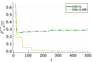
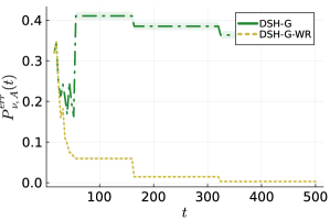
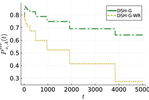
Figure 4: Empirical error on instances (a) NoA1, (b) IsA1, (c) Thr1, (d) RealL, (e) Med1 and (f) Thr3. “-WR” means that each SH instance keeps all its history instead of discarding it.

I.2.2 Fixed-budget Algorithms

We compare the fixed-budget performances of APGAI with the GAI versions SH-G and SR-G of SH and SR as described in Subsection I.2.1, the uniform round-robin strategy Unif, and different index policies in the prior knowledge-based meta algorithm PKGAI. Those index policies are defined in Section D and recalled below

PKGAI(APT_P) : $$i_{a}(t):=\sqrt{N_{a}(t)}(\hat{\mu}_{a}(t)-\theta)\>,\quad\text{PKGAI(UCB) : }i_{a}(t):=\hat{\mu}_{a}(t)-\theta+\sqrt{\frac{\beta(t)}{N_{a}(t)}}\>,$$

PKGAI(Unif) : $$i_{a}(t):=-N_{a}(t)\>,\quad\quad\quad\text{PKGAI(LCB-G) : }i_{a}(t):=\sqrt{N_{a}(t)}(\hat{\mu}_{a}(t)-\theta)+\sqrt{\beta(t)}\>.$$

Note that, contrary to APGAI and Unif, the other algorithms require the definition of the sampling budget $T$. For the sake of fairness, we do not use the theoretical value for $\beta$ as in Theorems 7 and 8. We implement the following confidence width, which is theoretically backed by Lemma 22 in Appendix G.2 (for $s=0$)

$$\beta(t)=\sigma\sqrt{z(T,\delta)/N_{a}(t)},\ \text{ where }z(T,\delta):=\overline{W}_{-1}(2\log(K/\delta)+2\log(2+\log T)+2),\text{ using $\delta=1\%$}\;.$$ (23)

We also consider for algorithms of the PKGAI family the theoretical threshold functions featured in Theorems 7 and 8, i.e.  relying on problem quantities in practice unavailable at runtime

$$\beta(t)=\sigma\sqrt{q(T,\delta)/N_{a}(t)},\ \text{ where }q(T,\delta):=\begin{cases}(T-K)/(4H_{1}(\mu))&\text{ if }\mathcal{A}_{\theta}(\mu)=\emptyset\\ (T-K)/(4K\hat{\Delta}^{-2})&\text{ otherwise }\end{cases}\;,$$ (24)

where $\hat{\Delta}:=\max_{a\in\mathcal{A}_{\theta}(\mu)}\Delta_{a}+\min_{b\not\in\mathcal{A}_{\theta}(\mu)}\Delta_{b}$.

I.2.3 Fixed-confidence Algorithms

Link Between GLR Stopping And UCB/LCB Stopping

In Kano et al., (2019), all the algorithms (HDoC, LUCB-G and APT-G) use a stopping rule which is based on UCB/LCB indices. Namely, they return an arm $a$ as soon as its associated LCB exceeds the threshold $\theta$. Since we consider GAI instead of AllGAI, this condition becomes a stopping rule. The second stopping condition is to return $\emptyset$ as soon as all the arms are eliminated, and an arm is eliminated when its UCB is lower than the threshold $\theta$. Direct manipulations show that the GLR stopping (5) is equivalent to their stopping provided that the UCB and LCB are using the same stopping threshold for the bonuses, i.e.

$$\max_{a\in\mathcal{A}}W^{+}_{a}(t)\geq\sqrt{2c(t,\delta)}\qquad\iff\qquad\exists a\in\mathcal{A},\quad\hat{\mu}_{a}(t)-\sqrt{\frac{2c(t,\delta)}{N_{a}(t)}}\geq\theta\>,$$

$$\min_{a\in\mathcal{A}}W^{-}_{a}(t)\geq\sqrt{2c(t,\delta)}\qquad\iff\qquad\forall a\in\mathcal{A},\quad\hat{\mu}_{a}(t)+\sqrt{\frac{2c(t,\delta)}{N_{a}(t)}}\leq\theta\>.$$

In Kano et al., (2019), they consider bonuses that only depend on the pulling count $N_{a}(t)$ instead of depending on the global time $t$. This ensures that the UCB remains constant once the arm has been eliminated. In contrast, using a UCB which depends on the global time $t$ (such as our stopping threshold in (6)) implies that this elimination step does not ensure that the condition on this arm still hold at stopping time. Mathematically, they use the following UCB/LCB

$$\hat{\mu}_{a}(t)\pm\sqrt{\frac{2\Lambda_{a}(t,\delta)}{N_{a}(t)}}\quad\text{where}\quad\Lambda_{a}(t,\delta)=\log(4K/\delta)+2\log N_{a}(t)\>.$$

Since Kano et al., (2019) consider Bernoulli distributions which are $1/2$-sub-Gaussian, we modified the bonuses to match the ones for $1$-sub-Gaussian (by using that the proper scaling is in $\sqrt{2\sigma^{2}}$).

While both stopping threshold $c$ and $(\Lambda_{a})_{a\in\mathcal{A}}$ have the same dominating $\delta$-dependency in $\log(1/\delta)$, it is worth noting that the time dependency of $c$ is significantly better since $c(t,\delta)\sim_{t\to+\infty}2\log\log t$. Ignoring the $\delta$-dependent terms and the constant, we have a lower bonus as long as $N_{a}(t)\gtrapprox\log t$. For a fair comparison, we will use the stopping threshold in (6) for the UCB/LCB used by HDoC and LUCB-G (both in the sampling and stopping rule) instead of the larger bonuses $(\Lambda_{a})_{a\in\mathcal{A}}$ considered in Kano et al., (2019).

Limits of Existing Algorithms

The APT-G algorithm introduced in Kano et al., (2019) samples

$$a_{t+1}=\arg\,\min_{a\in\mathcal{A}_{t}}\sqrt{N_{a}(t)}|\hat{\mu}_{a}(t)-\theta|\>,$$

where $\mathcal{A}_{t}$ is the set of active arms. This index policy is tailored for the Thresholding setting, where one needs to classify all the arms as above or below the threshold $\theta$. Intuitively, a good algorithm for Thresholding will perform poorly on the GAI setting since it must pay $H_{1}(\mu)$ even when $\mathcal{A}_{\theta}$. This is confirmed by the experiments in Kano et al., (2019), as well as our own experiments. Since it is not competitive, we omitted its empirical performance from our experiments.

The Sticky Track-and-Stop (S-TaS) algorithm introduced in Degenne and Koolen, (2019) admits a computationally tractable implementation for GAI. To the best of our knowledge, this is one of the few setting where this holds, e.g.  it is not tractable for $\varepsilon$-BAI. The major limitation of S-TaS lies in its dependency on an ordering $\mathcal{O}$ on the set of candidate answers $\mathcal{A}\cup\{\emptyset\}$. Informally, S-TaS computes a set of admissible answer based on a confidence region on the true mean, and sticks to the answer with the lowest ranking in the ordering $\mathcal{O}$. Then, S-TaS samples according to the optimal allocation for this specific answer. Depending on the choice of this ordering, the empirical performance can change drastically, especially for instances such that $\mathcal{A}_{\theta}(\mu)\neq\emptyset$. We consider two orderings to illustrate this. The Asc considers the ordering $\mathcal{O}$ such that $o_{a}=a$ for all $a\in\mathcal{A}$, and $a_{K+1}=\emptyset$. The Desc considers the ordering $\mathcal{O}$ such that $o_{a}=K-a+1$ for all $a\in\mathcal{A}$, and $a_{K+1}=\emptyset$. In Table 5, we can see that S-TaS performs considerably better for Asc compared to Desc. This can be explained by the fact that in all our instances the means are ordered, so that lower indices correspond to higher mean. Since higher means are easier to verify, this explains the improved performance for Asc.

Table 5: Empirical stopping time ($\pm$ standard deviation) of Sticky Track-and-Stop depending on the ordering on the set of candidate answers $\mathcal{A}\cup\{\emptyset\}$. “-” means that the algorithm didn’t stop after $10^{5}$ steps.

Ordering	Thr1	Thr2	Thr3	Med1	Med2	IsA1	IsA2	RealL
Asc	$183$	$435$	$11787$	$20488$	$114$	$120$	$33$	$341$
	$\pm 68$	$\pm 163$	$\pm 4539$	$\pm 7972$	$\pm 41$	$\pm 41$	$\pm 10$	$\pm 122$
Desc	$20574$	$19960$	$71057$	$60275$	$3087$	$16469$	$4539$	$-$
	$\pm 5835$	$\pm 5885$	$\pm 11684$	$\pm 16112$	$\pm 1293$	$\pm 4680$	$\pm 1434$	$-$

The Murphy Sampling (MS) algorithm introduced in Kaufmann et al., (2018) uses a rejection step on top of a Thompson Sampling procedure. For Gaussian instances, the posterior distribution $\Pi_{t,a}$ of the arm $a\in\mathcal{A}$ for the improper prior $\Pi_{0,a}=\mathcal{N}(0,+\infty)$ is $\Pi_{t,a}=\mathcal{N}(\hat{\mu}_{a}(t),1/\sqrt{N_{a}(t)})$. Let $\Pi_{t}=(\Pi_{t,a})_{a\in\mathcal{A}}$. Then, MS samples $\lambda\sim\Pi_{t}$ until $\max_{a\in\mathcal{A}}\lambda_{a}>\theta$, and samples arm $\arg\,\max_{a\in\mathcal{A}}\lambda_{a}$ for this realization. This rejection steps is equivalent to conditioning on the fact that $\mathcal{A}_{\theta}(\mu)\neq\emptyset$. As noted in Kaufmann et al., (2018), this rejection step can be computationally costly when $\mathcal{A}_{\theta}(\mu)=\emptyset$. Intuitively, we need to draw many vectors before observing $\lambda$ such that $\mathcal{A}_{\theta}(\lambda)\neq\emptyset$ once the posterior $\Pi_{t}$ has converged close to the Dirac distribution on $\mu$ when $\mathcal{A}_{\theta}(\mu)=\emptyset$. Empirically, we observed this phenomenon on the NoA2 instance. While all the other algorithms has a CPU running time of the order of $10$ milliseconds, MS reached a CPU running time of $10^{5}$ milliseconds.

We consider the Track-and-Stop (TaS) algorithm for GAI. It is direct to adapt the ideas of the original Track-and-Stop introduced in Garivier and Kaufmann, (2016) for BAI. When $\max_{a\mathcal{A}}\hat{\mu}_{a}(t)\geq\theta$, the optimal allocation $w^{\star}(\hat{\mu}(t))$ to be tracked is a Dirac in $\arg\,\max_{a\mathcal{A}}\hat{\mu}_{a}(t)$. Otherwise, using the proof of Lemma 1, the optimal allocation is $w^{\star}(\hat{\mu}(t))$, which is defined as

$$w^{\star}(\hat{\mu}(t))_{a}\propto(\hat{\mu}_{a}(t)-\theta)^{-2}\>.$$

On top of the C-Tracking procedure used to target the average optimal allocation, Track-and-Stop relies on a forced exploration procedure which samples under-sampled arms, i.e.  arms in $\{a\in\mathcal{A}\mid N_{a}(t)\leq\sqrt{t}-K/2\}$. Without the forced exploration, TaS would have worse empirical performance since it would be too greedy.

As mentioned in Sections 2 and 4, the BAEC meta-algorithm is only defined for asymmetric threshold $\theta_{U}>\theta_{L}$. Mathematically, it uses the following UCB/LCB indices

$$\hat{\mu}_{a}(t)+\sqrt{\frac{2\Lambda^{+}_{a}(t,\delta)}{N_{a}(t)}}\quad\text{where}\quad\Lambda^{+}_{a}(t,\delta)=\log\left(N(\delta)/\delta\right)\quad\text{and}\quad N(\delta):=\left\lceil\frac{2e}{(e-1)(\theta_{U}-\theta_{L})^{2}}\log\left(\frac{2\sqrt{K}}{(\theta_{U}-\theta_{L})^{2}\delta}\right)\right\rceil\>,$$

$$\hat{\mu}_{a}(t)-\sqrt{\frac{2\Lambda^{-}_{a}(t,\delta)}{N_{a}(t)}}\quad\text{where}\quad\Lambda^{-}_{a}(t,\delta)=\log\left(\sqrt{K}N(\delta)/\delta\right)\>.$$

In the GAI setting, those indices will infinite, hence BAEC is not defined properly. Instead of using asymmetric threshold, one could simply use symmetric ones which are independent of $(\theta_{U}-\theta_{L})^{-2}$. In that case, BAEC coincide with the HDoC and LUCB-G algorithms introduced in Kano et al., (2019).

I.2.4 Reproducibility

Experiments on Fixed-budget Empirical Error

The benchmark was implemented in Python 3.9, and run on a personal computer (configuration: processor Intel Core i$7-8750$H, $12$ cores @$2.20$GHz, RAM $16$GB). The code, along with assets for the real-life instance –where the exact treatment protocols have been replaced with placeholder names– are available in a .zip file under MIT (code) and Creative Commons Zero (assets) licenses. Commands which have generated plots and tables in this paper can be found in the Bash file named experiments.sh.

Experiments on Anytime Empirical Error and Empirical Stopping Time

Our code is implemented in Julia 1.9.0, and the plots are generated with the StatsPlots.jl package. Other dependencies are listed in the Readme.md. The Readme.md file also provides detailed julia instructions to reproduce our experiments, as well as a script.sh to run them all at once. The general structure of the code (and some functions) is taken from the tidnabbil library. This library was created by Degenne et al., (2019), see https://bitbucket.org/wmkoolen/tidnabbil. No license were available on the repository, but we obtained the authorization from the authors. Our experiments are conducted on an institutional cluster with $4$ Intel Xeon Gold 5218R CPU with $20$ cores per CPU and an x86_64 architecture.

I.3 Supplementary Results on Fixed-budget Empirical Error

Recall that we use here the prior-knowledge-agnostic threshold functions defined in Equation (23). We report in Figures 5, 6, 7, 8 and 9 the empirical error curves for all algorithms described in Subsection I.2.2 on real-life instance RealL, along with two synthetic instances IsA1 and IsA2 where $\mathcal{A}_{\theta}\neq\emptyset$, and two other instances where $\mathcal{A}_{\theta}=\emptyset$ (NoA1 and NoA2). Results are averaged over $1,000$ runs. In plots, we display the mean empirical error and shaded area corresponds to Wilson confidence intervals (Wilson,, 1927) with confidence $95\%$. Those Wilson confidence intervals are also reported on the corresponding tables.

In the real-life instance along with the instances with no good arms, uniform samplings (SH-G, SR-G, Unif and PKGAI(Unif)) are noticeably less efficient at detecting the presence or absence of good arms, contrary to the adaptive strategies. Moreover, except for instance IsA2, APGAI actually performs as well as more complex, elimination-based algorithms PKGAI($\star$), while allowing early stopping as well. Perhaps unsurprisingly, the performance of APGAI are closely related to those of PKGAI(APT_P), as both algorithms share the same sampling rule. In all three instances, although PKGAI has unrealistic assumptions in its theoretical guarantees (Theorems 7 and 8), its performance actually turns out to be the best of all algorithms. In particular, using the UCB sampling rule seems to be the most efficient. This shows that adaptive strategies can fare better than uniform samplings, which are more present in prior works in fixed-budget.

Performance on the Real-Life Application

We report empirical errors at $T=200$ in Table 6, at which budget empirical errors for all algorithms seem to converge (see Figure 5).

Table 6: Error across $1,000$ runs at $T=200$.

Algorithm	Error	Conf. intervals
APGAI	0.001	$2.10^{-4}\quad 6.10^{-3}$
PKGAI(APTP)	0.004	$2.10^{-3}\quad 0.01$
PKGAI(LCB-G)	0.001	$2.10^{-4}\quad 6.10^{-3}$
PKGAI(UCB)	0.000	$0.00\quad\quad 4.10^{-3}$
PKGAI(Unif)	0.001	$2.10^{-4}\quad 6.10^{-3}$
SH-G	0.005	$2.10^{-3}\quad 1.10^{-2}$
SR-G	0.002	$5.10^{-4}\quad 7.10^{-3}$
Unif	0.000	$0.00\quad\quad 4.10^{-3}$

Figure 5: Empirical error on instance RealL.

Performance on Synthetic Datasets ($\mathcal{A}_{\theta}\neq\emptyset$)

We report empirical errors at $T=700$ in Tables 7 and 8, at which budget empirical errors for all algorithms seem to converge (see Figures 6 and 7). In the figures, the curves of PKGAI(APT_P) and PKGAI(LCB-G) overlap.

Table 7: Error across $1,000$ runs at $T=700$.

Algorithm	Error	Conf. intervals
APGAI	0.003	$1.10^{-3}\quad 9.10^{-3}$
PKGAI(APTP)	0.004	$2.10^{-3}\quad 0.01$
PKGAI(LCB-G)	0.004	$2.10^{-3}\quad 0.01$
PKGAI(UCB)	0.000	$0.00\quad\quad 4.10^{-3}$
PKGAI(Unif)	0.000	$0.00\quad\quad 4.10^{-3}$
SH-G	0.000	$0.00\quad\quad 4.10^{-3}$
SR-G	0.000	$0.00\quad\quad 4.10^{-3}$
Unif	0.000	$0.00\quad\quad 4.10^{-3}$

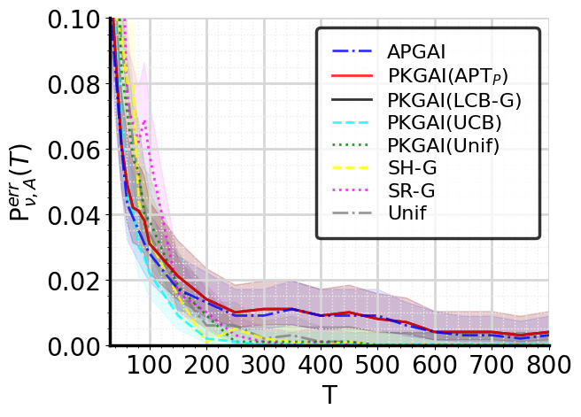
Figure 6: Empirical error on instance IsA1.

Table 8: Error across $1,000$ runs at $T=700$.

Algorithm	Error	Conf. intervals
APGAI	0.000	$0.00\quad 4.10^{-3}$
PKGAI(APTP)	0.000	$0.00\quad 4.10^{-3}$
PKGAI(LCB-G)	0.000	$0.00\quad 4.10^{-3}$
PKGAI(UCB)	0.000	$0.00\quad 4.10^{-3}$
PKGAI(Unif)	0.000	$0.00\quad 4.10^{-3}$
SH-G	0.000	$0.00\quad 4.10^{-3}$
SR-G	0.000	$0.00\quad 4.10^{-3}$
Unif	0.000	$0.00\quad 4.10^{-3}$

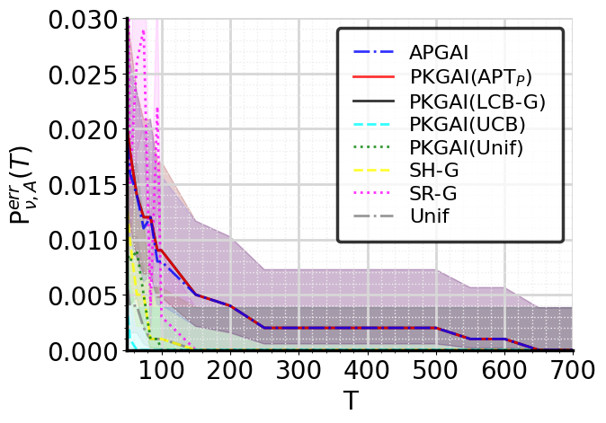
Figure 7: Empirical error on instance IsA2.

Performance on Synthetic Datasets ($\mathcal{A}_{\theta}=\emptyset$)

We report empirical errors at $T=150$ in Table 9 and $T=700$ in Table 10, at which budget empirical errors for all algorithms seem to converge (see Figures 8 and 9). In the figures, the curves of PKGAI(APT_P) and PKGAI(LCB-G) overlap.

Table 9: Error across $1,000$ runs at $T=150$.

Algorithm	Error	Conf. intervals
APGAI	0.000	$0.00\quad\quad 4.10^{-3}$
PKGAI(APTP)	0.000	$0.00\quad\quad 4.10^{-3}$
PKGAI(LCB-G)	0.000	$0.00\quad\quad 4.10^{-3}$
PKGAI(UCB)	0.000	$0.00\quad\quad 4.10^{-3}$
PKGAI(Unif)	0.002	$5.10^{-4}\quad 7.10^{-3}$
SH-G	0.000	$0.00\quad\quad 4.10^{-3}$
SR-G	0.007	$3.10^{-3}\quad 0.01$
Unif	0.005	$2.10^{-3}\quad 0.01$

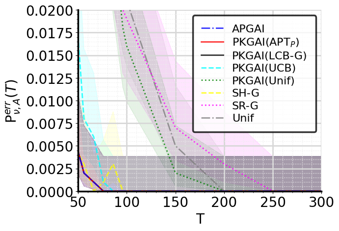
Figure 8: Empirical error on instance NoA1.

Table 10: Error across $1,000$ runs at $T=700$.

Algorithm	Error	Conf. intervals
APGAI	0.002	$5.10^{-4}\quad 7.10^{-3}$
PKGAI(APTP)	0.002	$5.10^{-4}\quad 7.10^{-3}$
PKGAI(LCB-G)	0.002	$5.10^{-4}\quad 7.10^{-3}$
PKGAI(UCB)	0.007	$3.10^{-3}\quad 0.01$
PKGAI(Unif)	0.021	$0.01\quad\quad 0.03$
SH-G	0.018	$0.01\quad\quad 0.03$
SR-G	0.127	$0.11\quad\quad 0.15$
Unif	0.084	$0.07\quad\quad 0.10$

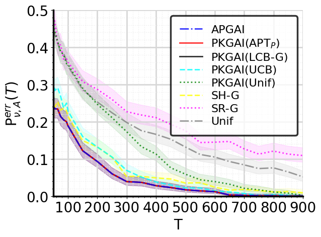
Figure 9: Empirical error on instance NoA2.

On Prior-Knowledge Based Threshold Functions

For the sake of completeness, we have also iterated those experiments using the prior-knowledge threshold functions (in practice, they are unavailable) in algorithms belonging to the PKGAI family.

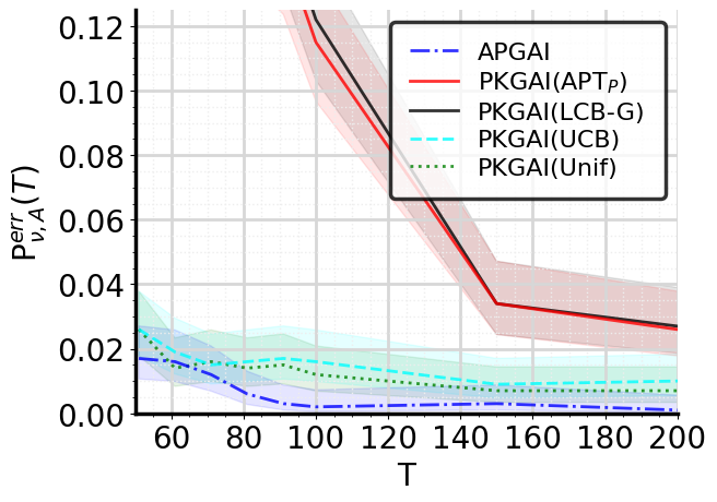
Figure 10: Empirical error on instance RealL. Left: with threshold functions from Equation (23). Right: with prior knowledge thresholds in Equation (24).

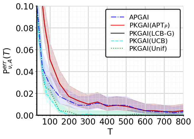
Figure 11: Empirical error on instance IsA1. Left: with threshold functions from Equation (23). Right: with prior knowledge thresholds in Equation (24).

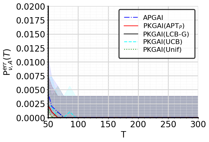
Figure 12: Empirical error on instance NoA1. Left: with threshold functions from Equation (23). Right: with prior knowledge thresholds in Equation (24).

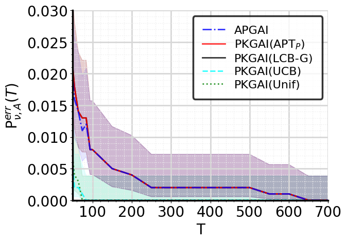
Figure 13: Empirical error on instance IsA2. Left: with threshold functions from Equation (23). Right: with prior knowledge thresholds in Equation (24).

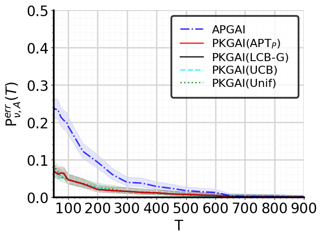
Figure 14: Empirical error on instance NoA2. Left: with threshold functions from Equation (23). Right: with prior knowledge thresholds in Equation (24).

In those figures, when plotting the empirical curves for PKGAI-like algorithms, we also report on the same plot the corresponding curve for our contribution APGAI (which is not expected to be different from the one on the left-hand plot, as the change in thresholds only affects PKGAI-like algorithms). As expected, the use of the prior-knowledge-based thresholds considerably improves the performance of PKGAI algorithms across most of the considered instances (except for RealL in Figure 10 where the performance of index policies APT_P and LUCB-G is severely impacted). However, more specifically in instances IsA2 (Figure 13), NoA1 (Figure 12), IsA1 (Figure 11) and RealL (Figure 10), we can notice that the gap in performance between APGAI and algorithms from the PKGAI (and more surprisingly, PKGAI(Unif)) is not very large. This means that the theoretical gap in Table 1 does not necessarily translate into practice and highlights the need for more refined tools for the analysis of these algorithms.

I.4 Supplementary Results on Anytime Empirical Error

Since we are interested in the empirical error holding for any time, we conly consider the anytime algorithms: APGAI, Unif, DSR-G and DSH-G. As mentioned in Appendix I.2, we consider the implementation DSH-G-WR (“without refresh‘’) which keeps all the history within each SH instance. We repeat our experiments over $10000$ runs. We display the mean empirical error and shaded area corresponds to Wilson confidence intervals (Wilson,, 1927) with confidence $95\%$.

In summary, our experiments show that APGAI significantly outperforms all the other anytime algorithms when $\mathcal{A}_{\theta}(\mu)=\emptyset$. When $\mathcal{A}_{\theta}(\mu)\neq\emptyset$, APGAI has always better performance than DSR-G and DSH-G, and it performs on par with Unif. Our empirical results suggest that APGAI enjoys better empirical performance than suggested by the theoretical guarantees summarized in Table 1.

Figure 15: Empirical error on instances (a) NoA1 and (b) NoA2. “-WR” means that each SH instance keeps all its history instead of discarding it.

No Good Arms

Since APGAI has arguably the best theoretical guarantees when $\mathcal{A}_{\theta}(\mu)=\emptyset$, we expect it to have superior empirical performance on the instances NoA1 and NoA2. Figure 15 validates empirically that APGAI significantly outperform all the other anytime algorithms by a large margin. While Unif has the “worse” theoretical guarantees in Table 1, the empirical study shows that it outperforms both DSR-G and DSH-G-WR. This phenomenon is mainly due to the doubling trick. Converting a fixed-budget algorithm to an anytime algorithm forces the algorithm to forget past observations, hence considerably impacting the empirical performance.

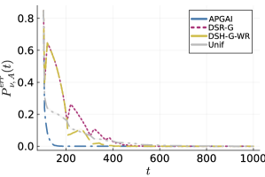
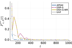
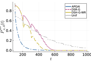
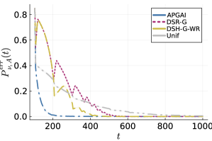
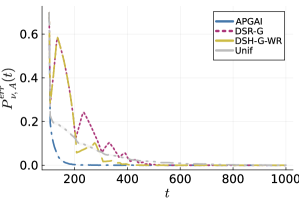
Figure 16: Empirical error for varying number of good arms $|\mathcal{A}_{\theta}(\mu)|\in\{5,15,30\}$ (left to right) among $K=100$ arms on instances (top) TwoG and (bottom) LinG. “-WR” means that each SH instance keeps all its history instead of discarding it.

Varying Number of Good Arms

In Figure 16, we study the impact of an increased number of good arms on the empirical error. While Table 1 suggests that APGAI is not benefiting from increased $|\mathcal{A}_{\theta}(\mu)|$, we see that the empirical error is decreasing significantly as $|\mathcal{A}_{\theta}(\mu)|$ increases. This suggests that better theoretical guarantees could be obtained when $\mathcal{A}_{\theta}(\mu)\neq\emptyset$. It is an interesting direction for future research to show an asymptotic rate featuring a complexity inversly proportional to $|\mathcal{A}_{\theta}(\mu)|$. In addition, we observe that APGAI outperforms all the other anytime algorithms by a large margin. Intuitively, APGAI is greedy enough when $\mathcal{A}_{\theta}(\mu)\neq\emptyset$ to avoid sampling the arms which are not good.

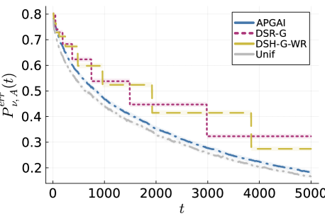
Figure 17: Empirical error on instances (a) Thr3 and (b) Med1. “-WR” means that each SH instance keeps all its history instead of discarding it.

Good Arms With Similar Gaps

In light of Table 1, one might expect that APGAI has worse empirical performance when $\mathcal{A}_{\theta}(\mu)\neq\emptyset$ compared to other anytime algorithms. To assess this fact empirically, we first consider instances where the good arms have similar gaps, e.g.  Thr3 and Med1. In Figure 17, we see that APGAI is better than Unif on Thr3, but worse on Med1. In both cases, APGAI outperforms both DSR-G and DSH-G-WR. Therefore, we see that APGAI has better empirical performance compared to the ones suggested by the theoretical guarantees summarized in Table 1.

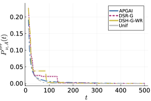
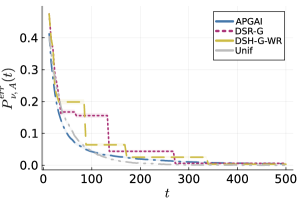
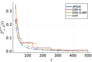
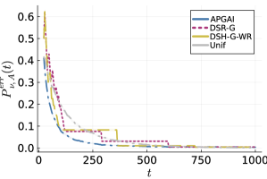
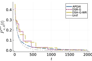
Figure 18: Empirical error on instances (a) IsA2, (b) Med2, (c) IsA1, (d) RealL, (e) Thr1 and (f) Thr2. “-WR” means that each SH instance keeps all its history instead of discarding it.

Good Arms With Dissimilar Gaps

In Figure 18, we consider instances where $\mathcal{A}_{\theta}(\mu)\neq\emptyset$ and good arms have dissimilar gaps. Overall, APGAI always performs better than DSR-G and DSH-G-WR. While Unif seems to outperform APGAI on some instances (e.g.  Thr2 and Med2), it has worse performance on other instances (e.g.  RealL and Thr1).

I.5 Supplementary Results on Empirical Stopping Time

While APGAI is designed to tackle anytime GAI, it also enjoys theoretical guarantees in the fixed-confidence setting when combined with the GLR stopping rule (5) with stopping threshold (6). According to Table 2, we expect that APGAI has good empirical performance when $\mathcal{A}_{\theta}(\mu)=\emptyset$, and sub-optimal ones when $\mathcal{A}_{\theta}(\mu)\neq\emptyset$. Since we are interested in the empirical performance for moderate regime of confidence, we take $\delta=0.01$ in the following. We repeat our experiments over $1000$ runs. We either display the boxplots or the mean with standard deviation as shaded area.

In summary, our experiments show that APGAI performs on par with all the other fixed-confidence algorithms when $\mathcal{A}_{\theta}(\mu)=\emptyset$. When $\mathcal{A}_{\theta}(\mu)\neq\emptyset$, APGAI has good performance only when the good arms have similar gaps. Importantly, its performance does not scale linearly with $|\mathcal{A}_{\theta}(\mu)|$ as suggested by Table 2. When good arms have dissimilar gaps, APGAI can suffer from large outliers due to the greedyness of it sampling rule. Finally, we shows a simple way to circumvent this limitation by adding forced exloration on top of APGAI.

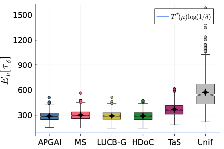
Figure 19: Empirical stopping time ($\delta=0.01$) on instances (a) NoA1 and (b) NoA2. “MS” is Murphy Sampling, “TaS” is Track-and-Stop and “Unif” is round-robin uniform sampling.

No Good Arms

Since APGAI is asymptotically optimal when $\mathcal{A}_{\theta}(\mu)=\emptyset$, we expect it to perform well on the instances NoA1 and NoA2. Figure 19 shows that APGAI has comparable performance with existing fixed-confidence GAI algorithms on such instances, and that uniform sampling performs poorly.

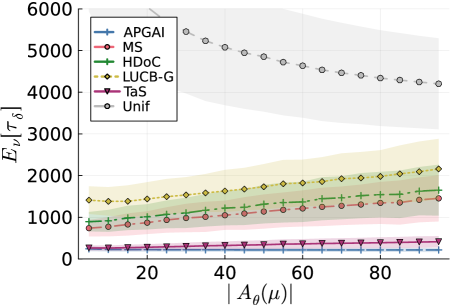
Figure 20: Empirical stopping time ($\delta=0.01$) for varying number of good arms $|\mathcal{A}_{\theta}(\mu)|\in\{5k\}_{k\in[19]}$ among $K=100$ arms on instances (a) TwoG and (b) LinG. “MS” is Murphy Sampling, “TaS” is Track-and-Stop and “Unif” is round-robin uniform sampling.

Varying Number of Good Arms

In Figure 20, we study the impact of an increased number of good arms on the empirical error. While Table 2 suggests that APGAI is suffering from increased $|\mathcal{A}_{\theta}(\mu)|$ due to the dependency in $H_{\theta}(\mu)$, we see that the empirical stopping time remains the same when $|\mathcal{A}_{\theta}(\mu)|\in\{5k\}_{k\in[19]}$. Therefore, Figure 20 empirically validate our theoretical intuition that APGAI can achieve an asymptotic upper bound of the order $2\max_{a\in\mathcal{A}_{\theta}(\mu)}\Delta_{a}^{-2}\log(1/\delta)$ as discussed in Appendix F.2.1. On the LinG, we also observe that APGAI can have large outliers due to the good arms with small gaps (see below for more details).

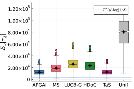
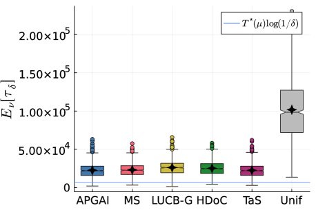
Figure 21: Empirical stopping time ($\delta=0.01$) on instances (a) Thr3 and (b) Med1. “MS” is Murphy Sampling, “TaS” is Track-and-Stop and “Unif” is round-robin uniform sampling.

Good Arms With Similar Gaps

When $\mathcal{A}_{\theta}(\mu)\neq\emptyset$ and good arms have similar means, Table 2 suggests that APGAI could be competitive with other algorithms. Figure 21 validates this observation empirically. On the Thr3 instance, APGAI achieves better performance than the other fixed-confidence algorithms, except for Track-and-Stop which has similar performance.

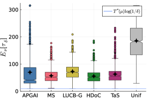
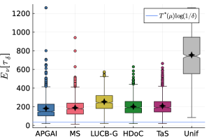
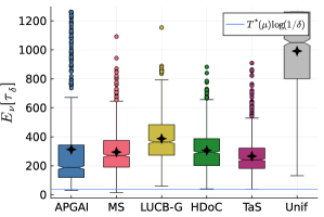
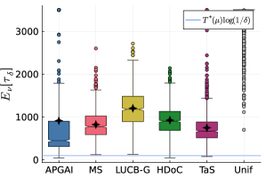
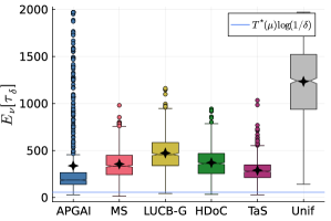
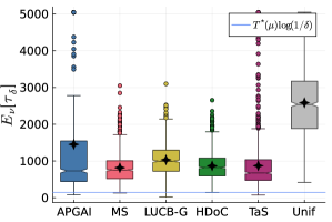
Figure 22: Empirical stopping time ($\delta=0.01$) on instances (a) IsA2, (b) Med2, (c) IsA1, (d) RealL, (e) Thr1 and (f) Thr2. “MS” is Murphy Sampling, “TaS” is Track-and-Stop and “Unif” is round-robin uniform sampling.

Good Arms With Dissimilar Gaps

In Figure 22, we consider instances where $\mathcal{A}_{\theta}(\mu)\neq\emptyset$ and good arms have dissimilar gaps. Table 2 suggests that APGAI can have poor empirical performance on such instances. Empirically, we see that APGAI can suffer from very large outliers on such instances. Depending on the initial draws, the greedy sampling rule of APGAI can focus on a good arm with small gap $\Delta_{a}$ instead of verifying a good arm with large gap $\Delta_{a}$. Since those arms are significantly harder to verify, APGAI will incur a large empirical stopping time in that case. This explains why the distribution of the empirical stopping time has an heavy tail with large outliers.

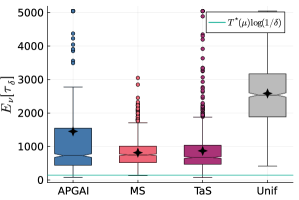
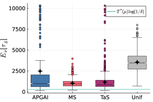
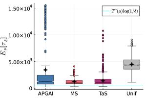
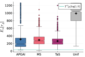
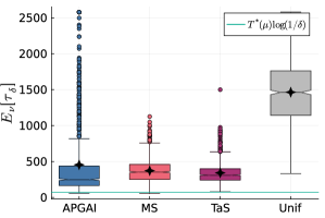
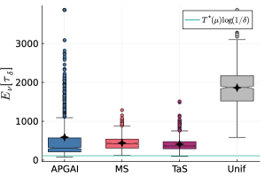
Figure 23: Empirical error for varying confidence level $\delta\in\{10^{-2},10^{-4},10^{-6}\}$ (left to right) on instances (top) Thr2 and (bottom) IsA1.

In Figure 23, we study the impact of a varying confidence level on instances where APGAI suffers from large outliers. For a fair comparison, we only consider fixed-confidence algorithm whose sampling rule is independent of $\delta$ (i.e.  excluding LUCB-G and HDoC). As expected, the large outliers phenomenon also increases when $\delta$ decreases.

Table 11: Empirical stopping time ($\pm$ standard deviation) of APGAI with (“-FE”) or without forced exploration.

Ordering	Thr1	Thr2	Thr3	Med1	Med2	IsA1	IsA2	RealL	NoA1	NoA2
APGAI	$634$	$2448$	$12301$	$22588$	$184$	$544$	$159$	$3721$	$288$	$3014$
	$\pm 2091$	$\pm 4269$	$\pm 4755$	$\pm 9204$	$\pm 147$	$\pm 1591$	$\pm 557$	$\pm 12511$	$\pm 56$	$\pm 1031$
APGAI-FE	$341$	$1466$	$12584$	$22394$	$216$	$341$	$72$	$921$	$287$	$3022$
	$\pm 505$	$\pm 2833$	$\pm 4818$	$\pm 8942$	$\pm 106$	$\pm 444$	$\pm 49$	$\pm 1389$	$\pm 55$	$\pm 1025$

Fixing APGAI With Forced Exploration

In the fixed-confidence setting, APGAI can suffer from large outliers when good arms have dissimilar means since it can greedily focus on good arms with small gaps. To fix this limitation, we propose to add forced exploration on top of APGAI, which we refer to as APGAI-FE. Let $\mathcal{U}_{t}=\{a\in\mathcal{A}\mid N_{a}(t)\leq\sqrt{t}-K/2\}$. When $\mathcal{U}_{t}\neq\emptyset$, we pull $a_{t+1}\in\arg\,\min_{a\in\mathcal{U}_{t}}N_{a}(t)$. When $\mathcal{U}_{t}\neq\emptyset$, we pull according to APGAI sampling rule.

Table 11 shows that adding forced exploration significantly reduce the mean and the variance of the stopping time on instances where APGAI was prone to large outliers. For instances where APGAI had no large outliers, APGAI-FE has the same empirical performance. Therefore, adding forced exploration allows to circumvent the empirical shortcomings of APGAI in the fixed-confidence setting.

References

- Audibert et al., (2010) Audibert, J.-Y., Bubeck, S., and Munos, R. (2010). Best arm identification in multi-armed bandits. In COLT, pages 41–53. Citeseer.
- Berry, (2006) Berry, D. A. (2006). Bayesian clinical trials. Nature reviews Drug discovery, 5(1):27–36.
- Carpentier et al., (2011) Carpentier, A., Lazaric, A., Ghavamzadeh, M., Munos, R., and Auer, P. (2011). Upper-confidence-bound algorithms for active learning in multi-armed bandits. In International Conference on Algorithmic Learning Theory.
- Degenne, (2019) Degenne, R. (2019). Impact of structure on the design and analysis of bandit algorithms. PhD thesis, Université de Paris.
- Degenne, (2023) Degenne, R. (2023). On the existence of a complexity in fixed budget bandit identification. In Proceedings of Thirty Sixth Conference on Learning Theory.