Non-defective degeneracy in non-Hermitian bipartite system and the realization in linear circuit

In terms of the random matrix theory, we simulate a non-Hermitian system in Gaussian orthogonal ensemble. Starting from a Hermitian operator with two distinct eigenvalues, we introduce the off-diagonal fluctuations through the random eigenkets, and realizing the bipartite nature through two $8\times 8$ subsystems, where one of them is full ranked, while the other is rank deficient. For the latter subsystem, we verify the non-defective degeneracy containing the non-linear symmetries, as well as the accumulation effect of the linear map in adjacent eigenvectors. Experimently, we observe such effect in a non-reciprocal non-Hermitian linear circuit.

1 Introduction

The Non-Hermitian physics can be implemented in optics of topological materials[7] and the electrical circuit[9], like the on-chip photonic circuit and nonreciprocal circuit. We consider two observables in our system, the first one is the $D$-dimensional randomly generated Hermitian matrix $H_{D}$ that is already in the quantum chaotic regime, whose ratio of variances (diagonal to off-diagonal) is closed to 2; The second one is constructed through elaborately prepared eigenbasis (eigenkets), where the corresponding eigenkets are selected from that of a real symmetric random matrix. As a result, we can obtain the matrix ${\bf M}$ whose entries are complex and read

$$M_{jj^{\prime}}=\sum_{\alpha}\lambda_{\alpha}\psi_{j}^{\alpha}(\psi_{j^{\prime}}^{\alpha})^{*},$$ (1)

where $\psi_{j}^{\alpha}$ is a vector instead of a trivial inner product (between the eigenstates of $H_{D}$ and that of the Hermitian operator $\hat{M}$). We note that, the past treatment for the generation of non-Hermiticity in ${\bf M}$ from the eigenkets of real symmetric random matrix is to consider the density operator (integrable eigenstates) of $\hat{M}$ as a summation of rank-1 matrices $M_{jj^{\prime}}=\sum_{k,l}\langle E_{j}|k\rangle\langle k|(\lambda_{\alpha}{\bf I})|l\rangle\langle l|E_{j^{\prime}}\rangle=\sum_{k}\lambda_{k}\langle E_{j}|k\rangle\langle k|E_{j^{\prime}}\rangle$, where the measurement of $\hat{M}$ in a non-Hermitian basis has a higher degrees of freedom in selecting the eigenkets. This treatment weaken the finite correlations between the original integrable eigenstates which is robust since they need to be mutually orthogonal and uniformly distributed with Haar measure. Although such correlations can be ignored in the limit of large dimension, i.e., ${\rm Rank}\hat{M}\rightarrow\infty$ due to the emergent statistically independence in the central limit, but it is not the case for a case with less flavor number like the case we discuss in this article that the Hermitian operator provides only two distinct finite eigenvalues. As a result, the resulting $\psi_{j}^{\alpha}$ (which is necessarily be a vector now) cannot be a real Gaussian distributed variable, but we found that it is able to share most features of a real Gaussian distributed variable (GOE here) even in the presence of finite correlation between two subsystems distincted by the eigenvalues of $\hat{M}$. We found that there is a clear correspondence between such correlations and the deviation of $\psi_{j}^{\alpha}$ from a real Gaussian variable, and such correlation can be revealed in terms of the emergent difference between the trace classes of two subsystems. With the degrees-of-freedom of the original Hermitian operator increase, there is level repulsion between all the subsystems except the one in end of spectrum. Correspondently, for these (bulk) subsystems ${\rm Rank}{\bf J}^{T}_{\alpha}{\bf J}_{\alpha}\rightarrow 1$ but there degenerated parts remain non-defective as long as the whole system is non-Hermitian (i.e., full-ranked). While in a linear circuit, the existence of non-Hermitian can simply be evidenced through the largest voltage response in one end, which can be directly observed by an obviously sink of voltage frequency and enhancement of voltage amplitude. Treating the time-dependent voltages as wave packets, its dynamics at the end node corresponds to the quantum evolution dominated by the full-ranked subsystem, $|V(t)\rangle=H\frac{d}{dt}|V(t)\rangle$.

2 Multisector

Next we conisder a thermalized Hamiltonian $M$ which containing $L$ nonlocal symmetry sectors labelled by ${\bf i}=1,\cdots,L$. For $\mathcal{H}_{j}$ as a variant of the Hermitian matrix $H_{j}$, is the $i$-th symmetry sectors of $M$, and its projector operator reads

$$\mathcal{P}_{i}=\sum_{j}(\langle E_{j}|{\bf J})^{T}(\langle E_{j}|{\bf J})=\sum_{j}{\bf J}^{T}|E_{j}\rangle\langle E_{j}|{\bf J}.$$ (2)

While for the $M$, its elements read

$$M_{jj^{\prime}}=\langle E_{j}|\hat{M}|E_{j^{\prime}}\rangle=\sum_{\alpha}\langle E_{j}|{\bf J}^{T}_{\alpha}(\lambda_{\alpha}{\bf I}){\bf J}_{\alpha}|E_{j^{\prime}}\rangle=\sum_{\alpha}\lambda_{\alpha}\psi_{j}^{\alpha}(\psi_{j^{\prime}}^{\alpha})^{*},$$ (3)

where we denote $\langle E_{j}|{\bf J}^{T}_{\alpha}=\psi_{j}^{\alpha}$ is an eigenvectors of $\mathcal{H}_{i}^{\alpha}$. ${\bf I}$ is the identity matrix. Thus for each nondegenerated eigenstate of ${\bf M}$, there is acoresponding $\mathcal{H}_{i}^{\alpha}$ whose trace is $\leq D$. To make sure the elements $M_{jj^{\prime}}$ satisfy the classical analog for the Gaussian variables in large system size, the matrices ${\bf J}_{\alpha}$ are formulated under the orthogonal and normalization conditions: $\psi_{j}^{\alpha}\psi_{j^{\prime}}^{\alpha*}=\delta_{jj^{\prime}},\ \overline{\psi_{j}^{\alpha}\psi_{j^{\prime}}^{\alpha*}}=\delta_{jj^{\prime}}\frac{1}{D},\ \sum_{j=1}^{D}|\psi_{j}^{\alpha}|^{2}=1\ (\forall\alpha)$.

To realize the eigenstate thermalization which follows the prediction of ETH, the Hermitian local observable $\hat{M}$ in the non-Hermitian basis provided by $H_{j}$ follows the classical analogy. For $\hat{M}$ with $\alpha_{m}$ nonzero distinct eigenvalues (each one corresponds to a unique integrable eigenstate), at least $\alpha_{m}$ eigenfunction $\psi_{j}^{\alpha}$ (i.e., $D\geq\alpha_{m}$) is needed for each eigenvalue (labelled by $\alpha$) of $\hat{M}$. That means there will be at least $\alpha_{m}^{2}$ eigenfunctions over all $\alpha$'s. Each eigenfunction $\psi_{j}^{\alpha}$ contains $D$ elements, where we only consider the case that $D(\geq\alpha_{m})$ and $\alpha_{m}$ are even integers. For the case $D=\alpha_{m}$, each eigenfunction caontains only the elements contributing to the non-fluctuation part, which plays the key role in the above-mentioned classical analogy and cannot be seem from an integrable eigenstate, if $D>\alpha_{m}$, there will be additionally $(D-\alpha_{m})=n\alpha_{m}\ (n\in\mathbb{Z})$ elements contributing the fluctuation part, which can be seem from an integrable eigenstate which cause large eigenvalue functuation in an integrable system by the high barrier that prohibiting the quantum transitions. Note that the vanishing transitions here reflect the negligibly correlation (or level repulsion) between quantum states of different symmetry sectors (usually labelled by good quantum numbers).

For $D=\alpha_{m}$, we arrange the eigenfunctions labelled by $j$'s to make the resulting eigenbasis satisfy

$$|\psi_{j}^{\alpha}|^{2}+|\psi_{j^{\prime}}^{\alpha}|^{2}=|\psi_{j}^{\alpha}|^{2}+|\psi_{j}^{\alpha^{\prime}}|^{2}=|\psi_{j}^{\alpha^{\prime}}|^{2}+|\psi_{j^{\prime}}^{\alpha^{\prime}}|^{2}=|\psi_{j^{\prime}}^{\alpha}|^{2}+|\psi_{j^{\prime}}^{\alpha^{\prime}}|^{2}.$$ (4)

which can be realized by the proper parameters in the nonfluctuation part. For $D-\alpha_{m}=n\alpha_{m}$, there will be $D=(n+1)\alpha_{m}$ eigenfunctions, which are statistically mutually independent, for each $\alpha$. Now these $D$ eigenfunctions (called the eigenbasis of $\alpha$) can be viewed as a collection of $(n+1)$ replicas of the variant of the corresponding eigenbasis at $D=\alpha_{m}$, i.e., in the new eigenbasis which including the fluctuation part, the elements contributing to the nonfluctuation part locate in the $1\cdots\alpha_{m}$, $(\alpha_{m}+1)\cdots 2\alpha_{m}$, $\cdots$, $(D-\alpha_{m}+1)\cdots(n+1)\alpha_{m}$, respectively, and we then classify the $\psi_{j}^{\alpha}$'s into these $(n+1)$ parts labelled by $k=1,\cdots,(n+1)$. We define

$$\psi_{k=1,q}^{\alpha}:=\psi^{\alpha}_{j=q},\ (1\leq q\leq\alpha_{m}),$$ (5)

$$\psi_{k=2,q}^{\alpha}:=\psi^{\alpha}_{j=\alpha_{m}+q},\ (\alpha_{m}+1\leq q\leq 2\alpha_{m}),$$

$$\cdots,$$

$$\psi_{k=(n+1),q}^{\alpha}:=\psi^{\alpha}_{j=n\alpha_{m}+q},\ (n\alpha_{m}+1\leq q\leq(n+1)\alpha_{m}).$$

Similar to Eq.(4), now the eigenbasis satisfies

$$|\psi_{kq}^{\alpha}|^{2}+|\psi_{kq^{\prime}}^{\alpha}|^{2}=|\psi_{kq}^{\alpha}|^{2}+|\psi_{kq}^{\alpha^{\prime}}|^{2}=|\psi_{kq}^{\alpha^{\prime}}|^{2}+|\psi_{kq^{\prime}}^{\alpha^{\prime}}|^{2}=|\psi_{kq^{\prime}}^{\alpha}|^{2}+|\psi_{kq^{\prime}}^{\alpha^{\prime}}|^{2},$$ (6)

$$|\psi_{kq}^{\alpha}|^{2}+|\psi_{k^{\prime}q}^{\alpha}|^{2}=|\psi_{kq^{\prime}}^{\alpha^{\prime}}|^{2}+|\psi_{k^{\prime}q^{\prime}}^{\alpha^{\prime}}|^{2}.$$

2.1 Bipartite system

For bipartite system, the averages over random eigenkets satisfy $\overline{\psi_{j}^{\alpha_{1}}\psi_{j}^{\alpha_{1}*}}=\overline{\psi_{j}^{\alpha_{2}}\psi_{j}^{\alpha_{2}*}}=\frac{1}{D},\overline{(\psi_{j}^{\alpha_{1}}\psi_{j}^{\alpha_{1}*})^{2}}=\overline{(\psi_{j}^{\alpha_{2}}\psi_{j}^{\alpha_{2}*})^{2}}=\frac{3}{D^{2}},\overline{\psi_{j}^{\alpha_{1}}\psi_{j}^{\alpha_{1}*}\psi_{j}^{\alpha_{2}}\psi_{j}^{\alpha_{2}*}}=\overline{\psi_{j}^{\alpha_{1}}\psi_{j}^{\alpha_{1}*}}\ \overline{\psi_{j}^{\alpha_{2}}\psi_{j}^{\alpha_{2}*}}=\frac{1}{D^{2}}\approx(\overline{\psi_{j}^{\alpha_{1}}\psi_{j}^{\alpha_{2}}\psi_{j}^{\alpha_{1}}\psi_{j}^{\alpha_{2}}})^{2}$, $\overline{\psi_{j}^{\alpha_{1}}\psi_{j^{\prime}}^{\alpha_{1}*}\psi_{j}^{\alpha_{2}}\psi_{j^{\prime}}^{\alpha_{2}*}}=\overline{\psi_{j}^{\alpha_{1}}\psi_{j^{\prime}}^{\alpha_{1}*}}\ \overline{\psi_{j}^{\alpha_{2}}\psi_{j^{\prime}}^{\alpha_{2}*}}=0$, $\overline{\psi_{j}^{\alpha_{1}}\psi_{j^{\prime}}^{\alpha_{1}*}}=\overline{\psi_{j}^{\alpha_{2}}\psi_{j^{\prime}}^{\alpha_{2}*}}=\overline{\psi_{j}^{\alpha_{1}}\psi_{j}^{\alpha_{2}*}}=0$. However, the off-diagonal parts of the two subsystems ${\bf\Psi}_{\alpha_{1}}$ and ${\bf\Psi}_{\alpha_{2}}$, which provide the non-Hermiticity, inevitably lead to: $\overline{\psi_{j}^{\alpha_{1}}\psi_{j^{\prime}}^{\alpha_{2}*}}\neq 0$, $\overline{\psi_{j}^{\alpha_{1}}\psi_{j^{\prime}}^{\alpha_{1}*}}=\overline{\psi_{j}^{\alpha_{2}}\psi_{j^{\prime}}^{\alpha_{2}*}}=0,\overline{(\psi_{j}^{\alpha_{1}}\psi_{j^{\prime}}^{\alpha_{1}*})^{2}}\neq\overline{(\psi_{j}^{\alpha_{2}}\psi_{j^{\prime}}^{\alpha_{2}*})^{2}}$, $\overline{(\psi_{j}^{\alpha_{1}}\psi_{j^{\prime}}^{\alpha_{1}*})^{2}+(\psi_{j}^{\alpha_{2}}\psi_{j^{\prime}}^{\alpha_{2}*})^{2}}=\frac{2}{D^{2}}$, $\overline{(\psi_{j}^{\alpha_{1}}\psi_{j^{\prime}}^{\alpha_{1}*})^{2}(\psi_{j}^{\alpha_{2}}\psi_{j^{\prime}}^{\alpha_{2}*})^{2}}\neq\overline{(\psi_{j}^{\alpha_{1}}\psi_{j^{\prime}}^{\alpha_{1}*})^{2}}\ \overline{(\psi_{j}^{\alpha_{2}}\psi_{j^{\prime}}^{\alpha_{2}*})^{2}}$ where the inequility is due to the finite correlation between the off-diagonal fourth moments of two subsystems.

$\overline{\psi_{j}^{\alpha_{1}}\psi_{j}^{\alpha_{1}}\psi_{j^{\prime}}^{\alpha_{1}}\psi_{j^{\prime}}^{\alpha_{1}}}=\overline{\psi_{j}^{\alpha_{2}}\psi_{j}^{\alpha_{2}}\psi_{j^{\prime}}^{\alpha_{2}}\psi_{j^{\prime}}^{\alpha_{2}}}=\frac{1}{D^{2}}+o(\frac{1}{D})$, where the error term decays with increasing system size, and evenly spread among all the subsystems, thus the decaying of error term here only contributes to the enhanced localizations in diagonal ensemble. In large system size limit, a collection of such localized states will be the discrete integrable states without the level repulsion between them. As a directe evidence, if we replace the intermediate matrices for each subsystem by the rank-1 matrices whose degenerated regions are defective (in large system size limit, the difference between defective rank-1 matrices and the non-defective rank-1 matrices only exhibited in the off-diagonal part), i.e., the matrices whose entries are $\langle E_{j}|\mathcal{J}_{\alpha_{1}}\rangle(\lambda_{\alpha}{\bf I})\langle\mathcal{J}_{\alpha_{1}}|E_{j^{\prime}}\rangle$ and $\langle E_{j}|\mathcal{J}_{\alpha_{2}}\rangle(\lambda_{\alpha}{\bf I})\langle\mathcal{J}_{\alpha_{2}}|E_{j^{\prime}}\rangle$, respectively, which are similar matrices, there off-diagonal variance will equal to the $\overline{\psi_{j}^{\alpha_{1}}\psi_{j}^{\alpha_{1}*}\psi_{j^{\prime}}^{\alpha_{1}}\psi_{j^{\prime}}^{\alpha_{1}*}}$ (or $\overline{\psi_{j}^{\alpha_{2}}\psi_{j}^{\alpha_{1}*}\psi_{j^{\prime}}^{\alpha_{1}}\psi_{j^{\prime}}^{\alpha_{2}*}}$), as a direct result of $|\mathcal{J}_{\alpha}\rangle=(|\psi_{1}^{\alpha}|,|\psi_{2}^{\alpha}|,\cdots,|\psi_{D}^{\alpha}|)^{T}$.

Thus the absence of non-defective degeneracies originates from the symmetry shape of the intermediate matrices ${\bf J}^{T}_{\alpha}{\bf J}_{\alpha}$ where the actural intermediate matrices (if available) should be weakly asymmetry. Such approximation results in the exact diagonalizability and leads to another exactly diagonalizable matrix, $\psi_{j}^{\alpha*}\psi_{j^{\prime}}^{\alpha}=\psi_{j^{\prime}}^{\alpha*}\psi_{j}^{\alpha}$, which in the mean time, artifically eliminate the inter-subsystems correlation (which should be exists for a bipartite system) through $\overline{\psi_{j}^{\alpha_{1}}\psi_{j^{\prime}}^{\alpha_{2}*}}=0$ or $\overline{(\psi_{j}^{\alpha_{1}}\psi_{j^{\prime}}^{\alpha_{1}*})^{2}(\psi_{j}^{\alpha_{1}}\psi_{j^{\prime}}^{\alpha_{1}*})^{2}}=\overline{(\psi_{j}^{\alpha_{1}}\psi_{j^{\prime}}^{\alpha_{1}*})^{2}}\ \overline{(\psi_{j}^{\alpha_{2}}\psi_{j^{\prime}}^{\alpha_{2}*})^{2}}$.

Thus base on a random matrix in quantum chaotic regime whose eigenvectors $|E_{j}\rangle$ provides the ingredients of such inavailability of an exact solution of ${\bf J}^{\alpha}$ implies that $\langle E_{j}|{\bf J}^{T}_{\alpha}=\psi_{j}^{\alpha}$ is indeed a Wigner-type expansion where the expansion coefficients necessarily carries the statistical properties of the chaotic systems[8] as a result of the coexistence of perturbed and unperturbed states. In other word, ${\bf J}^{T}_{\alpha}$ cannot be solved as a effective tensor here, but a functional type response whose exact form should contains infinite terms to exhausting the responses in all possible orders. In this sence, the unperturbed basis of the original Hermitian operator plays a less important role, compares to that of the intermediate term when the ingredient vectors $\psi_{j}^{\alpha}$ set in. But note that this statement is only valid in the case of few-subsystem. Such requirement for the expansion coefficients to be capable for different orders can be mitigated with the increasing number of subsystems.

2.2 Bipartite character within each subsystem supporting the diagonal-type conservation and off-diagonal type inter-subsystems correlation

The conservation within each subsystem only happen in diagonal channel, while the off-diagonal parts between different subsystems inevitably correlated While the level repulsions (in log scale) within the non-defective degenerate region for all the bulk subsystems will be more obvious with increasing number of subsystems, and meanwhile the non-defective degenerate region behaves more like an extensive summation that coupled with the nondegenerated region. Correspondenly, the enhanced level repulsion (in log scale) within each subsystem also leads to the mutually independence between bulk subsystems.

Thus, considering the coupling between degenerate and nondegenerate regions, there is finite correlation between them in the bipartite case, and such correlation enhanced with the increasing number of bulk subsystems, and meanwhile the non-Hermicity should be enhanced with the enhanced effect of level repulsion, but once such coupling over the critical value where the Hermicity appears in each bulk subsystem, which corresponds to the case that eaach bulk subsystem is simply a rank-1 matrix wthout any off-diagonal-type decorations in which case the ground states degenerated completely, the thermalization will be suppressed as a result of the emergent many-body localization (which behaves as system-size-independent). Correspondingly, such Hermitian-type degeneration cannot appears with increasing number of unit cells in our linear circuit (theoretically we can add infinite number of unit cells as far as it is within the range of op-amp gain), as the asymptotic degeneration can never equivalents to the defective degeneration with the increasing number of replicas, instead, changing the geometric of the linear circuit to breaks the bulk-end correspondence will leads to the Hermitian-type degeneration, in which case the linear enhancement of voltage frequencies nomore exists. Thus the slope of such frequency enhancement depends on the whole circuit instead of part of it, and such slope will be more sensitive to the whole circuit if we add more unit cells. Different to the case of nondegenerated thermalized spectrum, here the non-Hermicity does not reflected by the finite and distinct excited states in the spectrum, but through the orthogonal and self-normalized eigenvectors within the degenerated region.

3 Biorthogonality

In such a bipartite system, there will be a non-local symmetry sector with dimension $D_{NLS}=\frac{D}{2}-1$, i.e., an $D_{NLS}$-dimensional eigenspace spanned by the $D_{NLS}$ mutually orthogonal eigenvectors (and each one of them is able to form a orthogonal basis by themself) of ${\bf\Psi}_{\alpha_{1}}=\boldsymbol{\mathscr{S}}_{\alpha}\boldsymbol{\mathscr{S}}_{\alpha}^{T}$ that corresponding to zero eigenvalue. Note that $\alpha_{1}\notin\underline{\alpha}$. Such non-local symmetry sector is absent in another subsystem ${\bf\Psi}_{\alpha_{2}}$ which is full rank. The most essential characteristic of non-Hermiticity, which is the biorthogonality, is a result of the combination of these two subsysems.

In fact, Eq.(25) is completely true only for $\alpha=\alpha_{2}(\in\underline{\alpha})$, i.e., for full rank ${\bf\Psi}_{\alpha}$. For ${\bf\Psi}_{\alpha_{1}}$, there will be a $\frac{D}{2}\times\frac{D}{2}$ block filled by the real entrices (which only relate to the Hilbert dimension) equal to $\frac{1}{D}$, which is rank-one and thus supporting only one nonzero eigenvalue. However, as we mentioned above, ${\bf\Psi}_{\alpha_{1}}$ still has $D$ linear independent eigenvectors as its exactly diagonalizable, while $\boldsymbol{\uppsi}^{T}_{\alpha_{1}}\boldsymbol{\lambda}_{\alpha_{1}}[\boldsymbol{\uppsi}_{\alpha_{1}}^{T}]^{-1}$ and $\boldsymbol{\uppsi}^{-1}_{\alpha_{1}}\boldsymbol{\lambda}_{\alpha_{1}}\boldsymbol{\uppsi}_{\alpha_{1}}$ (see Eq.(25)) contain the block whose real part of the entries are the same with that of ${\bf\Psi}_{\alpha_{1}}$ but the distribution of imaginary parts (although vanishingly small; $\sim 10^{-10}$) are random and asymmetry. We call this block as random imaginary part block (RIB). Consequently, there are at most $(\frac{D}{2}+2)$ orthogonal eigenvectors for $\boldsymbol{\uppsi}^{T}_{\alpha_{1}}\boldsymbol{\lambda}_{\alpha_{1}}[\boldsymbol{\uppsi}_{\alpha_{1}}^{T}]^{-1}$ and $\boldsymbol{\uppsi}^{-1}_{\alpha_{1}}\boldsymbol{\lambda}_{\alpha_{1}}\boldsymbol{\uppsi}_{\alpha_{1}}$. Thus the minor random imaginary part in the RIB within a rank-deficient subsystem matrix will cause the reducing of nullspace's dimension from $(\frac{D}{2}-1)$ to 1 (geometric multiplicity of eigenvalue zero). In this case, there is a linear independent (full ranked) basis of eigenvectors for ${\bf\Psi}_{\alpha_{1}}$, which are, however, not mutually orthogonal. As a result, $\boldsymbol{\uppsi}_{\alpha_{1}}\boldsymbol{\uppsi}_{\alpha_{1}}^{T}$ is a diagonal matrix, but there are $(D-D_{NLS})$ diagonal entries smaller than one, and $D_{NLS}$ diagonal entries equal to one. That means the nullspace of ${\bf\Psi}_{\alpha_{1}}$ is spanned by $D_{NLS}$ non-orthogonal eigenvectors and each one of them form an orthogonal basis by itself.

For a bipartite non-Hermitian system constructed in above way, the NLS block (separated from ${\bf\Psi}_{\alpha_{1}}$) is of rank 1 and has the only nonzero eigenvalue equals to $(\frac{1}{2}-\frac{1}{D})$ (independent of $D$). Now due to the self-normalization and the mutual orthogonality (non-defective degeneracies by non-Hermiticity), the eigenvectors of NLS block are

$$\overbrace{(\sqrt{\frac{1}{2}},-\sqrt{\frac{1}{2}},0,\cdots,0)^{T}}^{D_{NLS}}$$ (7)

$$(-\sqrt{\frac{1}{6}},-\sqrt{\frac{1}{6}},\sqrt{\frac{1}{3}},0,\cdots,0)^{T}$$

$$\cdots,$$

$$(-\sqrt{\frac{1}{(D_{NLS}-1)D_{NLS}}},\cdots,-\sqrt{\frac{1}{(D_{NLS}-1)D_{NLS}}},\sqrt{\frac{D_{NLS}-1}{D_{NLS}}})^{T}$$

$$(-\sqrt{\frac{1}{D_{NLS}}},\cdots,-\sqrt{\frac{1}{D_{NLS}}})^{T},$$

where the non-Hermiticity can be seem from the last eigenvector which is the one related to the rest (nondegenerated) part of $\boldsymbol{\uppsi}_{\alpha_{1}}$.

We note that, the non-defective degeneracies in the NLS region as well as the non-Hermiticity relies on the coalesced but still robustly continued eigenvalues of the NLS block embeded into ${\bf\Psi}_{\alpha_{1}}$, which can be seem in Log scale. This is indeed necessary to keep the geometric multiplicity of the NLS block (nullspace) equals to $D_{NLS}$. Inevitably, $\frac{1}{\lambda_{\alpha_{1};i}}{\bf\Psi}_{\alpha_{1}}|{\bf\Psi}_{\alpha_{1};i}\rangle\neq|{\bf\Psi}_{\alpha_{1};i}\rangle$ for $i\in NLS$. In fact, within the NLS region, the above expression should becomes a functional derivative with the function $\lambda_{\alpha_{1};i}$

$$\frac{\delta{\bf\Psi}_{\alpha_{1}}|{\bf\Psi}_{\alpha_{1};i}\rangle}{\delta\lambda_{\alpha_{1};i}}=|{\bf\Psi}_{\alpha_{1};i}\rangle_{f},$$ (8)

can be realized by an eigenvalue-reparameterization transformation $\lambda_{\alpha_{1};i}\rightarrow f(\lambda_{\alpha_{1};i})$ with $f(\lambda_{\alpha_{1};i})$ a diffeomorphism $\lambda_{\alpha_{1};i}\rightarrow\lambda_{\alpha_{1};j}$. By considering the eigenvalues as the Lebesgue-Borel measure on Borel sets (the two measurable sets corresponding to the linear map of $f(\lambda_{\alpha_{1};i})$), and the derivative of $f(\lambda_{\alpha_{1};i})$ on $\lambda_{\alpha_{1};i}$ as a GL($D_{NLS}$,$\mathbb{R}$) mapping $\mathbb{R}^{D_{NLS}}\rightarrow\mathbb{R}^{D_{NLS}}$, the requirement of (monotonic) differentiability of the function $f(\lambda_{\alpha_{1};i})$ can be replaced by the invertibility of $f(\lambda_{\alpha_{1};i})$:

$$\frac{\delta{\bf\Psi}_{\alpha_{1}}|{\bf\Psi}_{\alpha_{1};i}\rangle_{f}}{\delta\lambda_{\alpha_{1};i}}=\frac{\partial{\bf\Psi}_{\alpha_{1}}|{\bf\Psi}_{\alpha_{1};i}\rangle_{f}}{\partial f(\lambda_{\alpha_{1};i})}\frac{\partial f(\lambda_{\alpha_{1};i})}{\partial\lambda_{\alpha_{1};i}}=\frac{\partial{\bf\Psi}_{\alpha_{1}}|{\bf\Psi}_{\alpha_{1};i}\rangle_{f}}{\partial f(\lambda_{\alpha_{1};i})}\frac{\lambda_{\alpha_{1};i}}{|{\rm Det}[\partial_{\lambda_{\alpha_{1};i}}f(\lambda_{\alpha_{1};i})]|},$$ (9)

where

$$f(\lambda_{\alpha_{1};i})=\frac{\lambda_{\alpha_{1};j}}{|{\rm Det}[\partial_{\lambda_{\alpha_{1};i}}f(\lambda_{\alpha_{1};i})]|\circ f(\lambda_{\alpha_{1};i})^{-1}},$$ (10)

$$|{\rm Det}[\partial_{\lambda_{\alpha_{1};i}}f(\lambda_{\alpha_{1};i})]|=f^{-1}(\lambda_{\alpha_{1};j})\lambda_{\alpha_{1};i}^{-1}.$$

Lebesgue-Borel measure on the Borel sets has the following property base on the invertible map $f$:

$$f(\lambda_{\alpha_{1};i}(\upalpha))=\lambda_{\alpha_{1};i}(f^{-1}(\upalpha))=\sum^{\upalpha}\frac{\lambda_{\alpha_{1};j}}{|{\rm Det}[\partial_{\lambda_{\alpha_{1};i}}f(\lambda_{\alpha_{1};i})]|\circ f^{-1}(\lambda_{\alpha_{1};i})},$$ (11)

where $\upalpha$'s denote the measurable subsets for the degenerated eigenvector labelled by $i$. Indeed, the diffeomorphism $f(\lambda_{\alpha_{1};i})$ as a bijection allow us to divide the eigenvalue $\lambda_{\alpha_{1};i}$ into subsets according to the emergent flavors within each degenerated eigenvector. As numerically shown in Fig.LABEL:3, for $D_{NLS}=3$ ($D=8$) there are three commutative subsets:

$$\frac{\partial{\bf\Psi}_{\alpha_{1}}|{\bf\Psi}_{\alpha_{1};i}\rangle_{f}}{\partial f(\lambda_{\alpha_{1};i}(\upalpha))}\frac{\partial f(\lambda_{\alpha_{1};i})}{\partial\lambda_{\alpha_{1};i}}=\left\{\begin{array}[]{ll}\lambda_{\alpha_{1};i}(\upalpha_{1})|{\bf\Psi}_{\alpha_{1};i-1}\rangle^{-1}_{1},\ \upalpha=\upalpha_{1},\\ {\bf\Psi}_{\alpha_{1}}|{\bf\Psi}_{\alpha_{1};i}\rangle,\ \upalpha=\upalpha_{2}\\ o(1),\ \upalpha=\upalpha_{3}\end{array}\right..$$ (12)

The reparameterization to the continuously differentiable map allow us to explain the non-Hermiticity as well as the non-defective degeneracies in NLS region by considering the degenerated eigenvectors (virtual) into several components that each represents a state with finite expectation (not the ground state) under the local symmetry with respect to the the eigenspace of this degenerated eigenvector. An extensive number of such mutually commutative virtual components is allowed like the possible generalized Gibbs ensemble in a nonintegrable system with an extensive number of local symmetries[5]. Each one of the components of a degenerated eigenvector can be classified into a flavor uniquely by the diffeomorphism-asisted differention on the nullspace eigenvalues whose distinct magnitudes can be seem in log scale (see Fig.2). In perspective of the robustly continuous spectrum even to the degenerated region, which exhibit the persistive level repulsion, there is indeed nonzero correlations between the subspace containing all the integrable eigenstates and that containing all the degenerated eigenstates (the nullspace). This is guaranteed by the extensive nature of these subspaces, where both of them are made up by local terms, and here the local terms refer to the mutually orthogonal eigenvectors (where the head elements plays an important role in keeping the level repulsion) in NLS block and the discrete eigenvalues outside the NLS block. Such continous feature exhibited in both the (rescaled) spectrum and the eigenvectors, related to the topological symmetries, is important in the study of topological materials, like the concepts of exceptional point (where both the eigenvalues and eigenvectors coalesce) or non-defective degeneracy point[6].

Eq.(LABEL:1051) is shown in Fig.LABEL:3, where the first line indicates that the impalpable correlations between eigenvectors relies on the first element, i.e., $\langle{\bf\Psi}_{\alpha_{1};i-1}|_{1}|{\bf\Psi}_{\alpha_{1};i}\rangle_{1}=\lambda_{\alpha_{1};i}$ ($i=\frac{D}{2}+1,\cdots,D$). This means that, despite the local components ($\upalpha_{2}$ and $\upalpha_{3}$ in Eq.(LABEL:1051)), the head element ($\upalpha_{1}$) results in special relation between eigenvectors $|{\bf\Psi}_{\alpha_{1};i}\rangle$ ($i=\frac{D}{2}+1,\cdots,D$), i.e., the orthogonality as well as the level repulsion (in log scale) for the corrresponding eigenvalues. However, the correlation for head elements does not cause correlation between arbitary two degenerated eigenvectors (which is for sure due to the extensive character of the subspace played by the whole nullspace). That is the reason why we using the smooth map, $f:\ \lambda_{\alpha_{1};i}\rightarrow\lambda_{\alpha_{1};j}$ ($i,j\in NLS$), to describe such relations between the degenerated eigenvectors. Correspondently, there is the differential $df:\ T(\lambda_{\alpha_{1};i})\mathbb{R}_{i}\rightarrow T(f(\lambda_{\alpha_{1};i}))\mathbb{R}_{j}$ ($i,j\in NLS$), which is the linear map as a result of the binary operation and at the best linear approximation. Here $T$ denotes the tangent space as a result of the derivative for original subset (an arbitarty eigenvector) to the $\mathbb{R}$, and thus the above differential is isomorphic to $\mathbb{R}_{i}\rightarrow\mathbb{R}_{j}$. Theoretically infinite-order derivative can be performed as the linear map in both subsets, and results in $df:\ \mathbb{R}\rightarrow\mathbb{R}$. In this process, the differential as a linear map replace the smooth map by the pushforward between the elements of an abelian group. With the order of differention move deeper (along the direction of a single subset), the isomorphism guarantees the resulting groups always be abelian. This equivalents to restricting the bijections to exist only between two adjacent subsets, which is to guarantees the commutative relation between bijections. Also, since the differential from the a subset to the next subset always equivalents to the derivation within the next subset, and using the first line of Eq.(LABEL:1051) which restricts that the head element always be determined by the last eigenvector, the invertibility of $f$ or $df$ (whose inversed forms are also continuously differentiable) will not cause the many-body localization of a single subset. This is analogous to the reciprocity breaking in a non-Hermitian circuit. In other word, for an arbitary subset within the NLS region, despite the invertible bijections, the complete localization for each subset is suppressed by the next subset,

This requires $f$ to be $C^{\infty}$ (infinite-times continuously) differentiable, and thus the resulting head elements of the degenerated eigenvectors will nearly exhibit not different which corresponds to the limit of asympototic degeneracy for the continuous spectrum where the level repusion is persistive. While in our case, we consider $f$ to be $C^{1}$-differentiable, and as a result there is level repulsion in log scale for the spectrum (see Fig.2) and the head element of the degenerated eigenvectors (as well as that of the $(\frac{D}{2}+1)$-th eigenvector which is adjacent to the NLS block) are correlated through the nearby linear map between arbitary two adjacent subsets (eigenvectors) and allow us to collect the degeneracies into an extensive quantity. Thus the linear map across single (or several) subsets equivalents to the derivative at the last subset where the best linear approximation sets in. In other word, the level repulsion (in log scale) within the degenerated region is due to the accumulation of linear map to different ends.

This can be simulated experimentally in a non-Hermitian linear circuit with broken reciprocity, where we simulate a monodirectional hopping one-dimensional model. This circuit contains eigen OP07 operational amplifiers where the source voltage (1V/1kHz) is applied in the noninverting input terminal, while the inverting input terminal is connected with the output terminal to realizing the unity-gain operation through the negative feedback. The nonreciprocity as well as the non-Hermiticity is verified through the largest voltage response in one end of the circuit. As shown in Fig.1, the circuit can be divided into eight unit cells, where each one contains a OP07 operational amplifier and a resistor locates next to it. Also, every resistors are connected to a capacitor towards the ground. Then there are two effective nodes in each unit cell, $A_{i}$ and $B_{i}$ ($i=1,\cdots,8$). Nodes $A_{i}$ locate between the output terminal of OP07 operational amplifier and the resistor. Nodes $B_{i}$ locate between the resistor and the input terminal of next OP07 operational amplifier. Our experiments show that, except the end node, the $A_{i}$ nodes exhibit location-independent character, whose values are at the same level with small noise through the whole circuit. This indicates the character of degenerated NLS region. While the $B_{i}$ nodes exhibit stronger unstable character, and the frequency has a nearly linear increasing tendency through the whole circuit. And at the end node (opposites to the one with largest voltage response), the frequency as well as the noise reaches the maximal value.

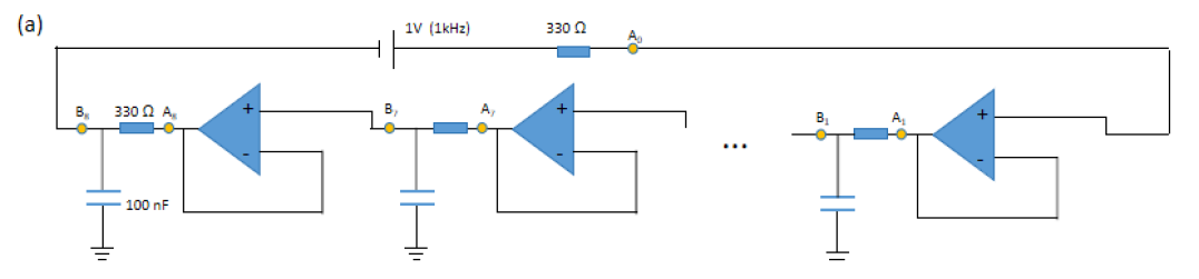
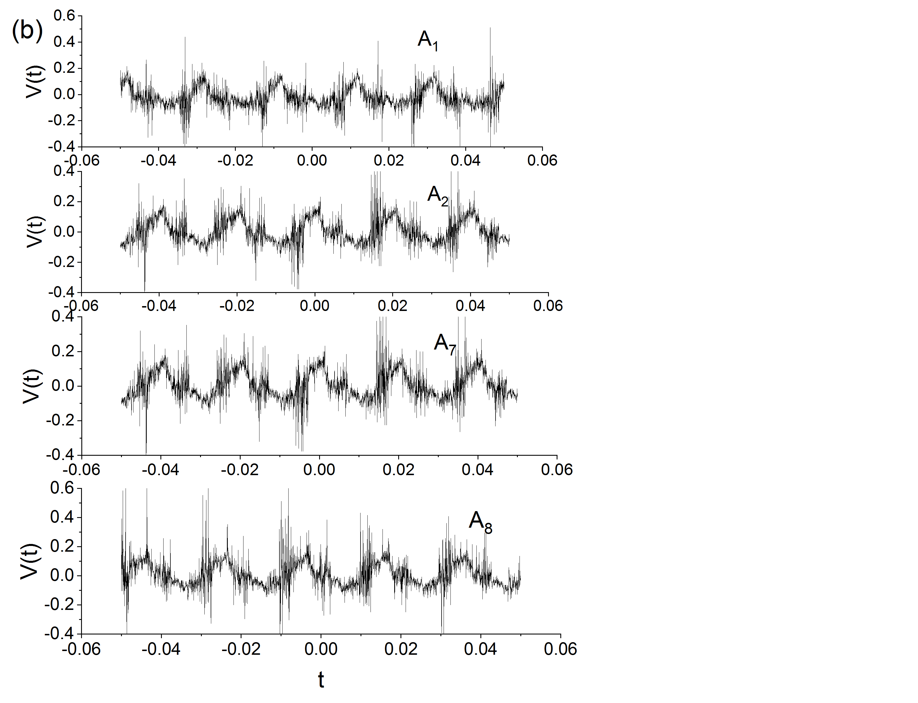
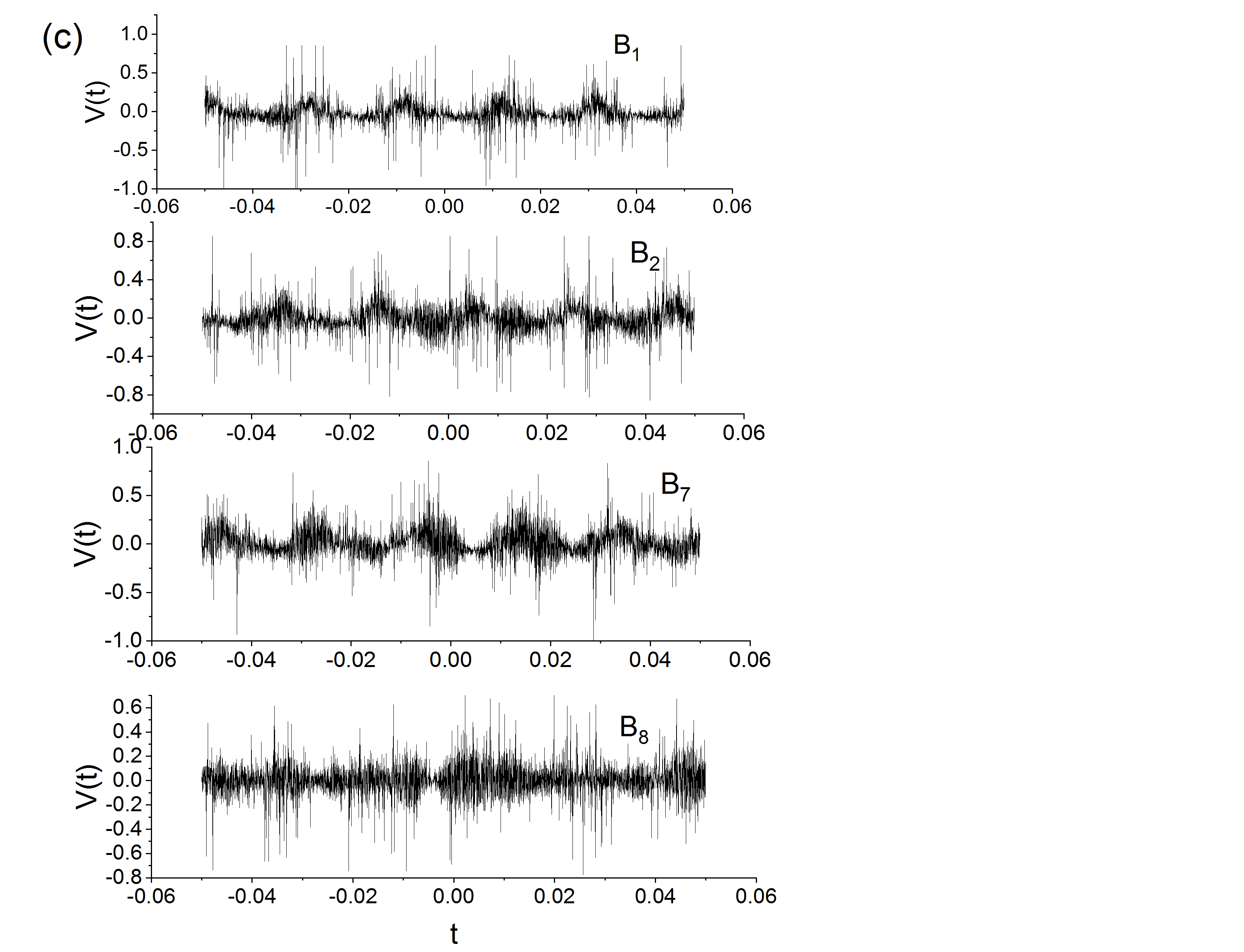
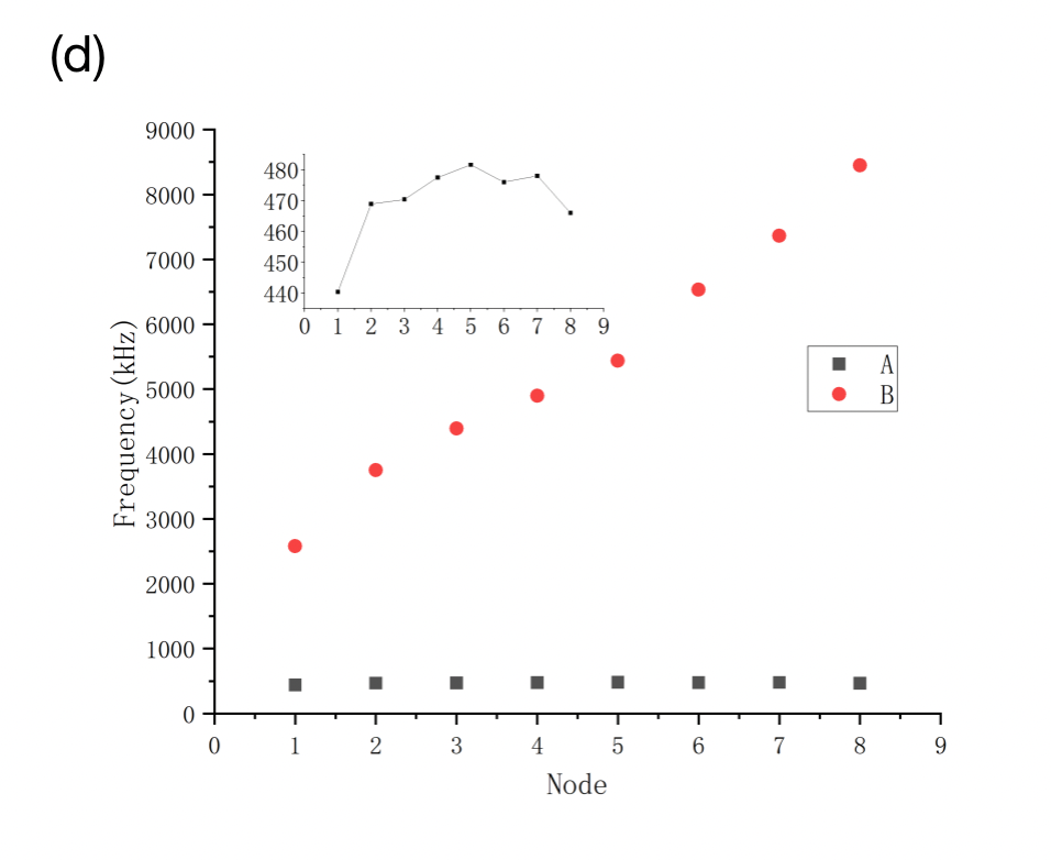
Figure 1: (a) Sketch of the linear circuit including eight nodes. (b) and (c) show the frequencies of voltage at $A$ and $B$ nodes. (d) shows the frequencies at all nodes. Datas for $A$ nodes are reploted in the insert to guide the eyes. For each operational amplifier we apply the dc voltages $\pm$ 13 V on the externalvoltage terminals. As an ideal op amp, the large input impedance (or equivalently, zero-admittance) guarantees the reciprocity breaking, As a result of perturbation from the resistor and capacitor after each Op amp, which leads to broaden the peaks in tehvoltage response and cause a unresolvable region[10]. Thus the increased frequencies in $B$ nodes can be regarded as nondegraded thermal noise, which keeping a obvious enhancement despite the capacitors have filtering part of the high frequencies from noise. While for the measurement at $A$ nodes, as far as it is within the bandwidth of operational amplifiers, Thus there is a linear increase of the resistance which plays teh role of (mutually independent) noise source. Next we explain how this circuit simulate the non-defective degenerated region of out system: When the source AC voltage pass the first resistor, the frequency measured at $A_{0}$ node is $\approx 150$ kHz, despite the unit gain effect, the non-Hermicity enforce a higher output frequency after the first op amp, which is $\approx 410$ kHz at $A_{1}$ node and exhibit a largest voltage amplitude here. After passing the second resistor, the frequency (at $B_{1}$ node) immediately over the gain bandwidth of opamp (600 kHz) which is $\approx 2600$ kHz and makes the unit gain effect fail after the fist op amp. The frequencies at $A_{1}\sim A_{8}$ are stable and locate around $460$ kHz, as a result of attenuation effect which is overwhelming over the enhancement during to the accumulated resistors. In the mean time, the minor effect due to the accumulation of resistors is persistent which guarantees the non-Hermicity and results in a gain higher than unit (about $\times 2.8$) at the edge node. In this linear circuit, the opamps with finite bandwidth play the role of source of non-Hermicity, which the series resistors with the same resistance provide the good local observable (see the discussion in Sec.), and the frequencies at $A$ nodes equivalent to the expectations of the replicas of the same non-Hermitian initial state with respect to the local observables, i.e., $330n$ $\Omega$ ($n=1\cdots 8$). Also, this is a $\mathcal{P}\mathcal{T}$-breaking circuit.

The summation over all the $\upalpha$-labelled subset of a certain degenerated eigenvector is essential in guaranteeing the above invertibility-related relation as well as the non-Hermiticity of whole system by enforcing the non-defective degeneracies in NLS region (this can be seem from Fig.5 according to the comparasion of eigenvector elements of ${\bf\Psi}_{\alpha_{1}}$ and ${\bf\Psi}_{\alpha_{2}}$).

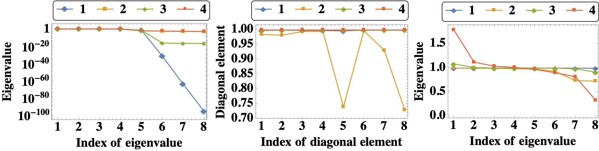
Figure 2: (a) 1,2,3,4 correspond to the absolute value of eigenvalues of of ${\bf\Psi}_{\alpha_{1}}$, ${\bf\Psi}_{\alpha_{2}}$, $\boldsymbol{\uppsi}^{-1}_{\alpha_{1}}\boldsymbol{\lambda}_{\alpha_{1}}\boldsymbol{\uppsi}_{\alpha_{1}}$, $\boldsymbol{\uppsi}^{-1}_{\alpha_{2}}\boldsymbol{\lambda}_{\alpha_{2}}\boldsymbol{\uppsi}_{\alpha_{2}}$ , respectively. (b) 1,2,3,4 correspond to the real part of diagonal elements of $\boldsymbol{\uppsi}_{\alpha_{1}}\boldsymbol{\uppsi}_{\alpha_{1}}^{T}$ $\boldsymbol{\uppsi}_{\alpha_{2}}\boldsymbol{\uppsi}_{\alpha_{2}}^{T}$ $\boldsymbol{\uppsi}_{\alpha_{1}}\boldsymbol{\uppsi}_{\alpha_{1}}^{H}$ $\boldsymbol{\uppsi}_{\alpha_{2}}\boldsymbol{\uppsi}_{\alpha_{2}}^{H}$, respectively. (c) 1,2,3,4 correspond to the eigenvalues of $\boldsymbol{\uppsi}_{\alpha_{1}}\boldsymbol{\uppsi}_{\alpha_{1}}^{T}$ $\boldsymbol{\uppsi}_{\alpha_{2}}\boldsymbol{\uppsi}_{\alpha_{2}}^{T}$ $\boldsymbol{\uppsi}_{\alpha_{1}}\boldsymbol{\uppsi}_{\alpha_{1}}^{H}$ $\boldsymbol{\uppsi}_{\alpha_{2}}\boldsymbol{\uppsi}_{\alpha_{2}}^{H}$, respectively. We see that the conjugate operation results in the normalized diagonal element and larger variance of eigenvalue. Also, Hermiticity can be seem from the eigenvalues depicted by 3,4 whose mean values equal to one, in contrast to depicted by 1,2 whose (real part of) mean values are 0.998387 and 0.992396, respectively.

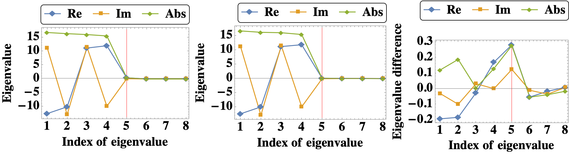
Figure 3: Eigenvalues of ${\bf\Psi}_{\alpha_{1}}$, ${\bf\Psi}_{\alpha_{2}}$, and their difference. Here we can see that, the effect of edge burst reflected in eigenvalues does not happen in the boundary of degenerated region,but the edge of nondegenerated region that closest to the degenerated region, i.e., the node $5$, where the most obvious level repulsion happen. While in the circuit of Fig.1(a), we can view the voltage source and the rest part of circuit as two coupled extensive quantities, thus the edge burst happened at $A_{1}$ node instead of the first node after the attenuation effect of op amp, i.e., $A_{2}$ node. That means $A_{1}$ and $A_{2}\sim A_{8}$ should be treated as mutually independent nodes with level repulsion between them, instead of two coupled extensive quantaties. Another evidence is that, there is no directly determination on the gain (above unit one) factor of first op amp by the collection of rest op amps, instead the $A_{1}\sim A_{8}$ as a collection coupled with the voltage source, and individually, the gain in node $A_{1}$ and that in nodes $A_{2}\sim A_{8}$ only determined by the whole circuit (whose local conservation can be verified using Kirchhoff's law) like the node number (shystem size). This also provide a scheme to observe the level repulsion beyond the non-degenerated spectrum, but a mixture of (non-defective) degenerated and non-degenerated region.

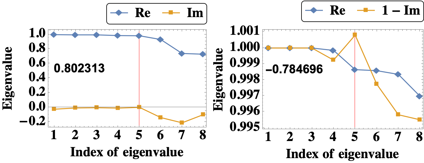
Figure 4: Eigenvalues of $\boldsymbol{\uppsi}_{\alpha_{1}}\boldsymbol{\uppsi}_{\alpha_{1}}^{T}$, $\boldsymbol{\uppsi}_{\alpha_{2}}\boldsymbol{\uppsi}_{\alpha_{2}}^{T}$. Since they are diagonal matrix, their eigenvalues are also their diagonal elements. Correlation between real and imaginary parts are indicated in each plot.

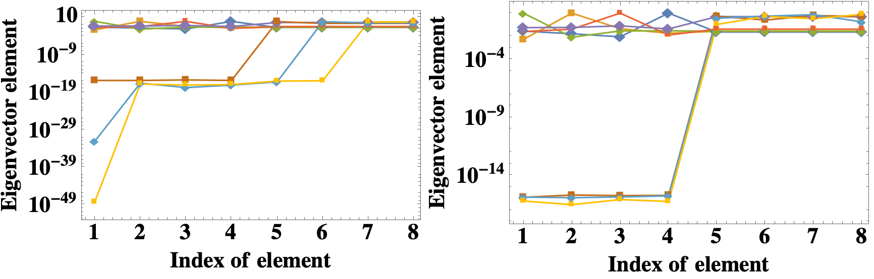
Figure 5: Elements of the eigenvectors of ${\bf\Psi}_{\alpha_{1}}$, $\boldsymbol{\uppsi}^{-1}_{\alpha_{1}}\boldsymbol{\lambda}_{\alpha_{1}}\boldsymbol{\uppsi}_{\alpha_{1}}$.

Similarly, for the full rank ${\bf\Psi}_{\alpha_{2}}$ which describes the another subsystem, there will also be a $\frac{D}{2}\times\frac{D}{2}$ block with real entries where the diagonal elements are $\frac{1}{D}$ and off-diagonal elements are $\frac{D-4}{D^{2}}$. Exactly diagonalization can be performed as $\boldsymbol{\uppsi}^{T}_{\alpha_{2}}\boldsymbol{\lambda}_{\alpha_{2}}[\boldsymbol{\uppsi}_{\alpha_{2}}^{T}]^{-1}$ and $\boldsymbol{\uppsi}^{-1}_{\alpha_{2}}\boldsymbol{\lambda}_{\alpha_{2}}\boldsymbol{\uppsi}_{\alpha_{2}}$, although have the RIB which is distinct from ${\bf\Psi}_{\alpha_{2}}$, have exactly the same eigenvectors with ${\bf\Psi}_{\alpha_{2}}$, i.e., $D$ mutually orthogonal eigenvectors, and thus $\boldsymbol{\uppsi}_{\alpha_{2}}\boldsymbol{\uppsi}_{\alpha_{2}}^{T}$ is a diagonal matrix with all diagonal entries smaller than one (due to the absence of orthogonal diagonalizability). It is easy to see that the absence of orthogonal diagonalizability (available in Hermitian case) here is due to the existence of imaginary parts of both the ${\bf\Psi}_{\alpha_{1}}$ and ${\bf\Psi}_{\alpha_{2}}$ (or in other word, the mixture of real and imaginary parts) as we are able to obtain a exact Hermitian basis by deviding ${\bf\Psi}_{\alpha}$ into ${\rm Re}[{\bf\Psi}_{\alpha}]$ and ${\rm Im}[{\bf\Psi}_{\alpha}]$, in which case $\widetilde{\boldsymbol{\uppsi}}_{\alpha}\widetilde{\boldsymbol{\uppsi}}_{\alpha}^{T}\equiv{\bf I}$ (here $\widetilde{\boldsymbol{\uppsi}}_{\alpha}$ is the matrix whose rows are the eigenvectors of ${\rm Re}[{\bf\Psi}_{\alpha}]$ or ${\rm Im}[{\bf\Psi}_{\alpha}]$).

Thus it is the collective effect of the real and imaginary part guarantees the exact equivalence between ${\bf\Psi}_{\alpha_{2}}$ and with its diagonalized forms (e.g., $\boldsymbol{\uppsi}^{T}_{\alpha_{2}}\boldsymbol{\lambda}_{\alpha_{2}}[\boldsymbol{\uppsi}_{\alpha_{2}}^{T}]^{-1}$ and $\boldsymbol{\uppsi}^{-1}_{\alpha_{2}}\boldsymbol{\lambda}_{\alpha_{2}}\boldsymbol{\uppsi}_{\alpha_{2}}$), and prevent the generation of NLS by the random imaginary parts in RIB. While such collective effect of the real and imaginary part is absent in rank deficient subsystem ${\bf\Psi}_{\alpha_{1}}$ due to the lacking of enough nonzero eigenvalues (expectations from observable ${\bf M}$) to avoiding the formation of orthogonal basis. In other word, the nondegenerated eigenvector corresponding to a nonzero eigenvalue, that doesnot form othrogonal basis by itself, identifying a certain mixture pattern between the real and imaginary parts of ${\bf\Psi}_{\alpha_{2}}$. Due to the same reason, the fluctuation of minor imaginary part in the RIB of ${\bf\Psi}_{\alpha_{1}}$ results in non-negligible asymmetry effect, i.e., ${\bf\Psi}_{\alpha_{1}}$ has a different eigenvector basis from its diagonalization representations (its eigendecomposed form).

The dissimilarity here is allowed by the $(\frac{D}{2}-1)$ nonunique eigenvectors that spanning the eigenspace corresponding to zero eigenvalue of ${\bf\Psi}_{\alpha_{1}}$, since there are more options for the entries distribution in the RIB that support a single nonzero eigenvalue, i.e., a unique eigenvector and other $(\frac{D}{2}-1)$ nonunique eigenvectors orthogonal to it.

3.1 Biorthogonality in terms of bipartite configuration

Due to the symmetry character of ${\bf\Psi}_{\alpha}$, a nonorthogonal inner product in off-diagonal basis is available from the nullspace eigenvectors of the ${\bf\Psi}_{\alpha_{1}}$ in decomposed representation (denoted as $\widetilde{{\bf\Psi}}_{\alpha_{1}}$ hereafter).

$$\langle\widetilde{{\bf\Psi}}_{\alpha_{1};i}|\widetilde{{\bf\Psi}}_{\alpha_{1}}^{{\dagger}}=x_{1}\langle\widetilde{{\bf\Psi}}_{\alpha_{1};i}|,$$ (13)

$$\langle\widetilde{{\bf\Psi}}^{{\dagger}}_{\alpha_{1};i}|\widetilde{{\bf\Psi}}_{\alpha_{1}}=x_{2}\langle\widetilde{{\bf\Psi}}_{\alpha_{1};i}^{{\dagger}}|,$$

where $\langle\widetilde{{\bf\Psi}}_{\alpha_{1};i}|$ and $\langle\widetilde{{\bf\Psi}}_{\alpha_{1};i}^{{\dagger}}|$ are the $i$-th eigenvectors of $\widetilde{{\bf\Psi}}_{\alpha_{1}}$ and $\widetilde{{\bf\Psi}}^{{\dagger}}_{\alpha_{1}}$, respectively. The only solution here is $x_{1}=x_{2}=0$, i.e., the eigenvectors labelled by $i$ are of the NLS (degenerated) part, which corresponds to the case of $\langle\widetilde{{\bf\Psi}}_{\alpha_{1};i}|\widetilde{{\bf\Psi}}_{\alpha_{1};j}^{{\dagger}}\rangle\neq 0\ (i\neq j)$[4]. The zero eigenvalues can be further verified in terms of the relation between the nonorthogonal inner product and the real/imaginary part of $\widetilde{{\bf\Psi}}_{\alpha_{1}}$[4] (for $i\neq j$),

$$\langle\widetilde{{\bf\Psi}}_{\alpha_{1};i}|\widetilde{{\bf\Psi}}_{\alpha_{1};j}\rangle=-2i\frac{\langle\widetilde{{\bf\Psi}}_{\alpha_{1};i}|{\rm Im}\widetilde{{\bf\Psi}}_{\alpha_{1}}|\widetilde{{\bf\Psi}}_{\alpha_{1};j}\rangle}{x_{1}-x_{0}}=2\frac{\langle\widetilde{{\bf\Psi}}_{\alpha_{1};i}|{\rm Re}\widetilde{{\bf\Psi}}_{\alpha_{1}}|\widetilde{{\bf\Psi}}_{\alpha_{1};j}\rangle}{x_{1}+x_{0}},$$ (14)

$$\langle\widetilde{{\bf\Psi}}_{\alpha_{1};i}^{{\dagger}}|\widetilde{{\bf\Psi}}_{\alpha_{1};j}^{{\dagger}}\rangle=-2i\frac{\langle\widetilde{{\bf\Psi}}_{\alpha_{1};i}^{{\dagger}}|{\rm Im}\widetilde{{\bf\Psi}}_{\alpha_{1}}|\widetilde{{\bf\Psi}}_{\alpha_{1};j}^{{\dagger}}\rangle}{x_{2}-x_{0}}=2\frac{\langle\widetilde{{\bf\Psi}}_{\alpha_{1};i}^{{\dagger}}|{\rm Re}\widetilde{{\bf\Psi}}_{\alpha_{1}}|\widetilde{{\bf\Psi}}_{\alpha_{1};j}^{{\dagger}}\rangle}{x_{2}+x_{0}}.$$

We can conclude that (for $i\neq j$)

$$\langle\widetilde{{\bf\Psi}}_{\alpha_{1};i}|\widetilde{{\bf\Psi}}_{\alpha_{1};j}\rangle=\langle\widetilde{{\bf\Psi}}_{\alpha_{1};i}^{{\dagger}}|\widetilde{{\bf\Psi}}_{\alpha_{1};j}^{{\dagger}}\rangle\left\{\begin{array}[]{ll}=0,\ i.j\notin NLS\\ \neq 0,\ i,j\in NLS\end{array}\right.,$$ (15)

$$\langle\widetilde{{\bf\Psi}}_{\alpha_{1};i}|\widetilde{{\bf\Psi}}_{\alpha_{1};j}^{{\dagger}}\rangle\left\{\begin{array}[]{ll}\neq 0,\ i.j\notin NLS\lor i,j\in NLS\\ =0,\ else\end{array}\right..$$

A significant feature for the subsystem containing the NLS block is $\langle\widetilde{{\bf\Psi}}_{\alpha_{1};i}|\widetilde{{\bf\Psi}}_{\alpha_{1};i}^{*}\rangle=1$ while $\langle\widetilde{{\bf\Psi}}_{\alpha_{1};i}|\widetilde{{\bf\Psi}}_{\alpha_{1};i}^{{\dagger}}\rangle\neq 1$. As an example, we have $\langle\widetilde{{\bf\Psi}}_{\alpha_{2};i}|\widetilde{{\bf\Psi}}_{\alpha_{2};i}^{*}\rangle=\langle\widetilde{{\bf\Psi}}_{\alpha_{2};i}|\widetilde{{\bf\Psi}}_{\alpha_{2};i}^{{\dagger}}\rangle=1$ for the full rank subsystem. That means the random imaginary part in RIB is able to (not able to) cause the asymmetry character of $\widetilde{{\bf\Psi}}_{\alpha_{1}}$ ($\widetilde{{\bf\Psi}}_{\alpha_{2}}$).

For $i.j\in NLS$, $\langle\widetilde{{\bf\Psi}}_{\alpha_{1};i}|\widetilde{{\bf\Psi}}_{\alpha_{1};j}^{*}\rangle=0$ is only possible for $x_{1}\neq x_{2}$. This requires more than two subsystems.

3.2 NLS block which contribute to the continuum part of the spectrum

The non-Hermitian conservation takes effect in the whole system but not just the NLS region.

Another significant character of the NLS in rank deficient subsystem can be seem from the combination effect between real and imaginary parts (which have nonzero correlations only in NLS block). The full rank subsystem ${\bf\Psi}_{\alpha_{1}}$ as well as the block separate from NLS block within ${\bf\Psi}_{\alpha_{2}}$, are all diagonal whose diagonal entries locates below one. Multiplying by the conjugate, ${\bf\Psi}_{\alpha}{\bf\Psi}_{\alpha}^{*}$, will change these diagonal blocks into non-diagonal blocks with the diagonal entries be replaced by one and the off-diagonal entries become nonzero. While in the decomposed representation, the rank deficient subsystem

$$\langle{\bf\Psi}_{\alpha_{1};i}|{\bf\Psi}_{\alpha_{1};j}^{*}\rangle\left\{\begin{array}[]{ll}1,\ i=j,\\ \neq 0,\ i.j\notin NLS\\ =0,\ else\end{array}\right..$$ (16)

$$\langle\widetilde{{\bf\Psi}}_{\alpha_{1};i}|\widetilde{{\bf\Psi}}_{\alpha_{1};j}^{*}\rangle\left\{\begin{array}[]{ll}1,\ i=j,\\ \neq 0,\ i.j\notin NLS\lor i,j\in NLS\\ =0,\ else\end{array}\right..$$

This allow us to coarse-graine the eigenvectors of and out of the NLS region into a single effective eigenvector,

$$\sum_{i\notin NLS}\langle{\bf\Psi}_{\alpha_{1};i}|\cdot\sum_{j\notin NLS}|{\bf\Psi}_{\alpha_{1};j}^{*}\rangle=\sum_{i,j\notin NLS}\langle{\bf\Psi}_{\alpha_{1};i}|{\bf\Psi}_{\alpha_{1};j}^{*}\rangle\approx\frac{D}{2}+1,$$ (17)

$$\sum_{i\notin NLS}\langle{\bf\Psi}_{\alpha_{1};i}|\cdot\sum_{j\in NLS}|{\bf\Psi}_{\alpha_{1};j}^{*}\rangle=\sum_{i\in NLS}\langle{\bf\Psi}_{\alpha_{1};i}|\cdot\sum_{j\notin NLS}|{\bf\Psi}_{\alpha_{1};j}^{*}\rangle=\sum_{i\notin NLS,j\in NSL}\langle{\bf\Psi}_{\alpha_{1};i}|{\bf\Psi}_{\alpha_{1};j}^{*}\rangle=\sum_{i\in NLS,j\notin NSL}\langle{\bf\Psi}_{\alpha_{1};i}|{\bf\Psi}_{\alpha_{1};j}^{*}\rangle=0,$$

which are still valid by replacing ${\bf\Psi}_{\alpha_{1};i}$ by $\widetilde{{\bf\Psi}}_{\alpha_{1};i}$.

$$\sum_{i\in NLS}\langle{\bf\Psi}_{\alpha_{1};i}|\cdot\sum_{j\in NLS}|{\bf\Psi}_{\alpha_{1};j}^{*}\rangle=\sum_{i,j\in NLS}\langle{\bf\Psi}_{\alpha_{1};i}|{\bf\Psi}_{\alpha_{1};j}^{*}\rangle\approx\frac{D}{2}-1,$$ (18)

$$\sum_{i\in NLS}\langle\widetilde{{\bf\Psi}}_{\alpha_{1};i}|\cdot\sum_{j\in NLS}|\widetilde{{\bf\Psi}}_{\alpha_{1};j}^{*}\rangle=\sum_{i,j\in NLS}\langle\widetilde{{\bf\Psi}}_{\alpha_{1};i}|\widetilde{{\bf\Psi}}_{\alpha_{1};j}^{*}\rangle\neq\frac{D}{2}-1,$$

i.e., the off-diagonal eigenvector products in NLS region of $\widetilde{{\bf\Psi}}_{\alpha_{1}}$ fail in the long-time thermalization (unlike ${\bf\Psi}_{\alpha_{1}}$), and the only way to make the subsystem $\widetilde{{\bf\Psi}}_{\alpha_{1}}$ be thermalized is the large number of NLS blocks (with distinct eigenvalues which may vanishingly small), in which case each DLS block has the dimension $D_{NLS}\rightarrow 1$, and the resulting subsystem with largest number of NLS blocks will be a rank-1 (and also trace-1) matrix.

The first line in Eq.(LABEL:9201) requires longer time fluctuations (or higher accuracy in the diagnosis of off-diagonal ETH) in the NLS region, since the mutually orthogonality between the eigenvectors within nullspace of ${\bf\Psi}_{\alpha_{1}}$ (as guaranteed by the exactly diagonalizability as well as the symmetry distribution of the entries). That means with a certain cutoff for the error, each eigenstate outside the NLS region is more localized with respect to others. As an evidence, the vanishing off-diagonal ($i\neq j$) product, $\langle{\bf\Psi}_{\alpha_{1};i}|{\bf\Psi}_{\alpha_{1};j}\rangle=\langle{\bf\Psi}_{\alpha_{1};i}|(|{\rm Re}\ {\bf\Psi}_{\alpha_{1};j}\rangle+|i{\rm Im}\ {\bf\Psi}_{\alpha_{1};j}\rangle)=0$ for every $i,j\notin NLS$, results from $\langle{\bf\Psi}_{\alpha_{1};i}|{\rm Re}\ {\bf\Psi}_{\alpha_{1};j}\rangle=-\langle{\bf\Psi}_{\alpha_{1};i}||i{\rm Im}\ {\bf\Psi}_{\alpha_{1};j}\rangle)\neq 0$. While for $i,j\in NLS$, we have $\langle{\bf\Psi}_{\alpha_{1};i}|{\rm Re}\ {\bf\Psi}_{\alpha_{1};j}\rangle=\langle{\bf\Psi}_{\alpha_{1};i}||i{\rm Im}\ {\bf\Psi}_{\alpha_{1};j}\rangle)=0$.

From the Eq.(LABEL:9211) and the first line of Eq.(LABEL:9201), we can obtain the normalization in terms of the effective eigenvectors $\langle{\bf\Psi}_{\alpha_{1};i}^{eff}|{\bf\Psi}_{\alpha_{1};j}^{*\ eff}\rangle\approx\delta_{ij}$, where $\langle{\bf\Psi}_{\alpha_{1};i}^{eff}|=\frac{1}{\sqrt{D_{i}}}\sum_{i}\langle{\bf\Psi}_{\alpha_{1};i}|,\ |{\bf\Psi}_{\alpha_{1};i}^{*\ eff}\rangle=\frac{1}{\sqrt{D_{i}}}\sum_{i}|{\bf\Psi}_{\alpha_{1};i}^{*}\rangle$. We also notice that, the non-defective degeneracies only exist in the NLS block, where the eigenvectors therein exactly satisfy $\langle{\bf\Psi}_{\alpha_{1};i}|{\bf\Psi}_{\alpha_{1};j}\rangle=\delta_{ij}$, where the bar and ket here are usually distincted by the left and right states in terms of the biorthogonal configuration in a system that completely consist of such kind of eigenvector (instead of only a block within it). Since in our system, there is a $(\frac{D}{2}-1)\times(\frac{D}{2}-1)$ NLS block with zero eigenvalues, Different to the system that completely consist of biorthogonal eigenvectors, the non-defective degeneracies here is more likely be pretected by the above-mentioned trace classes instead of some certain non-Hermitian-type symmetries. We numerically verify that (for $i\neq j$ and $i,j\in NLS$)

$${\rm Tr}[|{\bf\Psi}_{\alpha_{1};i}\rangle\langle{\bf\Psi}_{\alpha_{1};j}^{*}|-|{\bf\Psi}_{\alpha_{1};j}\rangle\langle{\bf\Psi}_{\alpha_{1};i}^{*}|]=0,$$ (19)

$${\rm Rank}[|{\bf\Psi}_{\alpha_{1};i}\rangle\langle{\bf\Psi}_{\alpha_{1};j}^{*}|-|{\bf\Psi}_{\alpha_{1};j}\rangle\langle{\bf\Psi}_{\alpha_{1};i}^{*}|]={\rm Rank}[(|{\bf\Psi}_{\alpha_{1};i}\rangle\langle{\bf\Psi}_{\alpha_{1};j}^{*}|-|{\bf\Psi}_{\alpha_{1};j}\rangle\langle{\bf\Psi}_{\alpha_{1};i}^{*}|)^{2}]=2,$$

$$(|{\bf\Psi}_{\alpha_{1};i}\rangle\langle{\bf\Psi}_{\alpha_{1};j}^{*}|-|{\bf\Psi}_{\alpha_{1};j}\rangle\langle{\bf\Psi}_{\alpha_{1};i}^{*}|)|{\bf\Psi}_{\alpha_{1};i}\rangle=-|{\bf\Psi}_{\alpha_{1};j}\rangle,$$

$$(|{\bf\Psi}_{\alpha_{1};i}\rangle\langle{\bf\Psi}_{\alpha_{1};j}^{*}|-|{\bf\Psi}_{\alpha_{1};j}\rangle\langle{\bf\Psi}_{\alpha_{1};i}^{*}|)|{\bf\Psi}_{\alpha_{1};j}\rangle=|{\bf\Psi}_{\alpha_{1};i}\rangle,$$

$$(|{\bf\Psi}_{\alpha_{1};i}\rangle\langle{\bf\Psi}_{\alpha_{1};j}^{*}|-|{\bf\Psi}_{\alpha_{1};j}\rangle\langle{\bf\Psi}_{\alpha_{1};i}^{*}|)^{2}|{\bf\Psi}_{\alpha_{1};j}\rangle=-|{\bf\Psi}_{\alpha_{1};j}\rangle,$$

$$(|{\bf\Psi}_{\alpha_{1};i}\rangle\langle{\bf\Psi}_{\alpha_{1};j}^{*}|-|{\bf\Psi}_{\alpha_{1};j}\rangle\langle{\bf\Psi}_{\alpha_{1};i}^{*}|)^{2}|{\bf\Psi}_{\alpha_{1};i}\rangle=-|{\bf\Psi}_{\alpha_{1};i}\rangle,$$

$${\rm Tr}[(|{\bf\Psi}_{\alpha_{1};i}\rangle\langle{\bf\Psi}_{\alpha_{1};j}^{*}|-|{\bf\Psi}_{\alpha_{1};j}\rangle\langle{\bf\Psi}_{\alpha_{1};i}^{*}|)^{2}]={\rm Tr}[(|{\bf\Psi}_{\alpha_{1};i}\rangle\langle{\bf\Psi}_{\alpha_{1};j}^{*}|-|{\bf\Psi}_{\alpha_{1};j}\rangle\langle{\bf\Psi}_{\alpha_{1};i}^{*}|)(|{\bf\Psi}_{\alpha_{1};i}\rangle\langle{\bf\Psi}_{\alpha_{1};j}^{*}|-|{\bf\Psi}_{\alpha_{1};j}\rangle\langle{\bf\Psi}_{\alpha_{1};i}^{*}|)^{*}]=-2$$

$$=-{\rm Tr}[(|{\bf\Psi}_{\alpha_{1};i}\rangle\langle{\bf\Psi}_{\alpha_{1};j}^{*}|-|{\bf\Psi}_{\alpha_{1};j}\rangle\langle{\bf\Psi}_{\alpha_{1};i}^{*}|)(|{\bf\Psi}_{\alpha_{1};i}\rangle\langle{\bf\Psi}_{\alpha_{1};j}^{*}|-|{\bf\Psi}_{\alpha_{1};j}\rangle\langle{\bf\Psi}_{\alpha_{1};i}^{*}|)^{{\dagger}}].$$

where the last line reflects different feature from the system that completely consist of biorthogonal eigenvectors in which case the corresponding symmetry operator is antiunitary whose square is $-{\bf I}$[2]. Such non-defective degeneracies are destroyed by the decomposition in terms of the (quasi)-diagonal ensemble, and except the above-mentioned (Eq.(LABEL:9301)) loss of orthogonality between eigenvectors within NLS block (defective degeneracies)

$${\rm Tr}[(|\widetilde{{\bf\Psi}}_{\alpha_{1};i}\rangle\langle\widetilde{{\bf\Psi}}_{\alpha_{1};j}^{*}|-|\widetilde{{\bf\Psi}}_{\alpha_{1};j}\rangle\langle\widetilde{{\bf\Psi}}_{\alpha_{1};i}^{*}|)^{2}]\approx-2,$$ (20)

whose values fluctuate around -2. Another feature related to the non-Hermitian physics, is the degenerated eigenstates (non-defective degeneracy) contributing to the continuous spectrum of the scattering states (rather than the completely coalesced defective degeneracy), where in large N limit the non-fermi liquid (replica-diagona) will lead to coalesced IR (long-time) poles that forming a branch cut along imaginary axis. Such singularity as well as the absence of fermi liquid (well-defined quasi particle) is related to the existence of strong scatterers[3]. Also, the IR pole is cuted off before vanish by the continuu spectrum which means the system owns a self oscillation frequency (at the saddle point).

4 Conclusion

In terms of the non-reciprocal linear map in the degenerated matrix block (towards the nondegenerated one) and the derivative of Lebesgue measurement, we verify the unidirectional accumulation effect of the boundary-dependence for the degenerated eigenvectors which form the nonlocal symmetry region.

We found that, compares to the defective degeneracies where the degenerated eigenvectors loss the self-normalization and mutually orthogonality, there is roubust accumulation effect of the non-Hermicity toward the nondegenerated matrix block where each eigenvcetors (mutually orthogonal but not self-normalized) corresponds to a distinct nonzero eigenvalue. In log scale, the continued spectrum can be observed in the NLS region, and as a result, the correlations between an eigenvector $|{\bf\Psi}_{\alpha_{1};i}\rangle$ and the collection of the rest part $\sum_{j=i+1}^{D}|{\bf\Psi}_{\alpha_{1};j}\rangle$ is always proportional to the expectation of the subsystem ${\bf\Psi}_{\alpha_{1}}$ on it. And as another evidence of the non-reciprocity, the correlations between $|{\bf\Psi}_{\alpha_{1};i}\rangle$ and its rest $\sum_{j=i+1}^{D}|{\bf\Psi}_{\alpha_{1};j}\rangle$ is always dominating over the $|{\bf\Psi}_{\alpha_{1};i+1}\rangle$ and its rest $\sum_{j=i+2}^{D}|{\bf\Psi}_{\alpha_{1};j}\rangle$, which is an unique phenomenon in the non-defective degenerated block. In perspective of the Lebesgue measurement, this can be explained by the longer time accumulation (toward the equilibrium) for the former compares to the latter. The robust non-defective degeneration originates from the robust level repulsion between the local states locates in the middle of spectrum. Analogically, we realize and simulate such phenomenon in a one-dimensional non-Hermitian linear circuit using the simple linear components: capacitor, resistor, and operational amplifer. In terms of the unidirectional and robust nearly linear increase of frequency and the signal noise for the nodes within each unit cell from one end to another end of the circuit. By virtue of the finite open-loop gain of operational amplifier, we observe such level repulsion which can be observed only under the measure of lower magnitude.

5 Appendix

6 diagnosis in terms of diagonal ETH and diagonal ensemble

Concequently, $\sum_{j\leq j^{\prime}}\psi_{j}^{\alpha}(\psi_{j^{\prime}}^{\alpha})^{*}=\sum_{j\leq j^{\prime}}\psi_{j}^{\alpha}(\psi_{j^{\prime}}^{\alpha})^{*}=1$. Next we denote $\boldsymbol{\mathscr{S}}_{\alpha}$ as the square matrix whose rows are the eigenvectors $\psi_{j}^{\alpha}$ arranged in order of $j$ ($1,\cdots,D$). Then with respect to the symmetry matrix ${\bf J}_{\alpha}^{T}{\bf J}_{\alpha}$,

$${\rm Rank}[\sum_{\alpha}^{\alpha_{m}}{\bf J}_{\alpha}{\bf J}_{\alpha}^{T}]=D,$$ (21)

$${\rm Rank}[{\bf J}_{\alpha}]={\rm Rank}[{\bf J}^{T}_{\alpha}{\bf J}_{\alpha}]={\rm Rank}[{\bf J}_{\alpha}{\bf J}_{\alpha}^{T}]={\rm Rank}[\boldsymbol{\mathscr{S}}_{\alpha}]={\rm Rank}[\boldsymbol{\mathscr{S}}_{\alpha}\boldsymbol{\mathscr{S}}^{T}_{\alpha}]={\rm Rank}[\boldsymbol{\mathscr{S}}^{T}_{\alpha}\boldsymbol{\mathscr{S}}_{\alpha}]={\rm Rank}[\boldsymbol{\mathscr{S}}_{\alpha}\boldsymbol{\mathscr{S}}^{H}_{\alpha}]={\rm Rank}[\boldsymbol{\mathscr{S}}^{H}_{\alpha}\boldsymbol{\mathscr{S}}_{\alpha}]\leq D,$$

$${\rm Tr}[{\bf J}_{\alpha}{\bf J}_{\alpha}^{T}]={\rm Tr}[{\bf J}_{\alpha}^{T}{\bf J}_{\alpha}]={\rm Tr}[\boldsymbol{\mathscr{S}}_{\alpha}\boldsymbol{\mathscr{S}}^{T}_{\alpha}]={\rm Tr}[\boldsymbol{\mathscr{S}}^{T}_{\alpha}\boldsymbol{\mathscr{S}}_{\alpha}]=1,\ {\rm Tr}[{\bf J}_{\alpha}{\bf J}_{\alpha}^{H}]={\rm Tr}[{\bf J}_{\alpha}^{H}{\bf J}_{\alpha}]={\rm Tr}[\boldsymbol{\mathscr{S}}_{\alpha}\boldsymbol{\mathscr{S}}^{H}_{\alpha}]={\rm Tr}[\boldsymbol{\mathscr{S}}^{H}_{\alpha}\boldsymbol{\mathscr{S}}_{\alpha}]\neq 1,\ \ (\forall\alpha)$$

$${\rm Rank}[|E_{j}\rangle\langle E_{j^{\prime}}|]=1,{\rm Rank}[\sum_{j}|E_{j}\rangle\langle E_{j}|]={\rm Tr}[\sum_{j}|E_{j}\rangle\langle E_{j}|]={\rm Tr}[\sum_{jj^{\prime}}|E_{j}\rangle\langle E_{j^{\prime}}|]={\rm Tr}[\sum_{j\leq j^{\prime}}|E_{j}\rangle\langle E_{j^{\prime}}|]={\rm Rank}[\sum_{j\leq j^{\prime}}|E_{j}\rangle\langle E_{j^{\prime}}|]=D,$$

$${\rm Rank}[\sum_{jj^{\prime}}|E_{j}\rangle\langle E_{j^{\prime}}|]=1,\ {\rm Tr}[\sum_{j}|E_{j}\rangle\langle E_{j}|]=D,\ {\rm Rank}[\sum_{jj^{\prime}}|E_{j}\rangle\langle E_{j^{\prime}}|]=1,\ {\rm Tr}[|E_{j}\rangle\langle E_{j^{\prime}}|]=\delta_{jj^{\prime}},$$

where for $j\neq j^{\prime}$ the resulting matrix $|E_{j}\rangle\langle E_{j^{\prime}}|$ is an nilpotent matrix, as an outer product of two orthogonal eigenstates. For convinience, next we denote the matrix ${\bf\Psi}_{\alpha}:=\boldsymbol{\mathscr{S}}_{\alpha}\boldsymbol{\mathscr{S}}_{\alpha}^{T}(\neq\boldsymbol{\mathscr{S}}_{\alpha}^{T}\boldsymbol{\mathscr{S}}_{\alpha})$, whose elements are $\psi_{j}^{\alpha}(\psi_{j^{\prime}}^{\alpha})^{*}$.

Further, since $\sum_{j}(\psi_{j}^{\alpha})^{*}\psi_{j}^{\alpha}=\boldsymbol{\mathscr{S}}_{\alpha}^{T}\boldsymbol{\mathscr{S}}_{\alpha}$,

$${\rm Rank}[\sum_{j}(\psi_{j}^{\alpha})^{*}\psi_{j}^{\alpha}]={\rm Rank}[\sum_{j\leq j^{\prime}}(\psi_{j}^{\alpha})^{*}\psi_{j^{\prime}}^{\alpha}]\leq D,\ {\rm Rank}[\sum_{jj^{\prime}}(\psi_{j}^{\alpha})^{*}\psi_{j^{\prime}}^{\alpha}]=1,$$ (22)

$${\rm Tr}[\sum_{j}(\psi_{j}^{\alpha})^{*}\psi_{j}^{\alpha}]={\rm Tr}[\sum_{j\leq j^{\prime}}(\psi_{j}^{\alpha})^{*}\psi_{j^{\prime}}^{\alpha}]={\rm Tr}[\sum_{jj^{\prime}}(\psi_{j}^{\alpha})^{*}\psi_{j^{\prime}}^{\alpha}]=1,\ (\forall\alpha)$$

For the rank-one matrices $\sum_{jj^{\prime}}(\psi_{j}^{\alpha})^{*}\psi_{j^{\prime}}^{\alpha}$, the only one nonzero eigenvalue is one, and corresponding to a one-dimensional eigenspace. As symmetry matrix which is diagonalizable, each eigenvalue of $\sum_{jj^{\prime}}(\psi_{j}^{\alpha})^{*}\psi_{j^{\prime}}^{\alpha}$ has the geometric multiplicity equals the algebraic multiplicity, thus the eigenspace of zero eigenvalues is $(D-1)$.

$$\sum_{jj^{\prime}}(\psi_{j}^{\alpha})^{*}\psi_{j^{\prime}}^{\alpha}=\ell_{i}^{T}(\frac{|\ell_{1}|}{|\ell_{i}|},\cdots,\frac{|\ell_{D}|}{|\ell_{i}|})=(\frac{|\ell_{1}|}{|\ell_{i}|},\cdots,\frac{|\ell_{D}|}{|\ell_{i}|})^{T}\ell_{i},$$ (23)

$$\ell_{i}(\frac{|\ell_{1}|}{|\ell_{i}|},\cdots,\frac{|\ell_{D}|}{|\ell_{i}|})^{T}=(\frac{|\ell_{1}|}{|\ell_{i}|},\cdots,\frac{|\ell_{D}|}{|\ell_{i}|})\ell_{i}^{T}=1,$$

where $\ell_{i}\ (i\leq D)$ is the $i$-th row of matrix $\sum_{jj^{\prime}}(\psi_{j}^{\alpha})^{*}\psi_{j^{\prime}}^{\alpha}$. Then in terms of the eigenvector $\ell_{1}$ corresponding to the only one nonzero eigenvalue, which can be expressed as linear scalings of arbitary $\ell_{i}$ or $(\frac{|\ell_{1}|}{|\ell_{i}|},\cdots,\frac{|\ell_{D}|}{|\ell_{i}|})$,

$$\sum_{jj^{\prime}}(\psi_{j}^{\alpha})^{*}\psi_{j^{\prime}}^{\alpha}\ell_{1}^{T}=\ell_{1}^{T}=\ell_{i}\ell_{1}^{T}(\frac{|\ell_{1}|}{|\ell_{i}|},\cdots,\frac{|\ell_{D}|}{|\ell_{i}|})^{T}=(\frac{|\ell_{1}|}{|\ell_{i}|},\cdots,\frac{|\ell_{D}|}{|\ell_{i}|})\ell_{1}^{T}\ell_{i}^{T}.$$ (24)

The results about the rank which is possible to smaller than $D$ in Eqs.(LABEL:8111,LABEL:8112) indicates that the projector operators into the corresponding sector (for each integrable eigenstates) may not completely mutually orthogonal. We also note that, all the matrices ${\bf\Psi}_{\alpha}$ (for different $\alpha$) are symmetry, and thus be orthogonally diagonalizable (non-defective, but no the normal matrix), i.e.,

$${\bf\Psi}_{\alpha}=\boldsymbol{\uppsi}^{T}_{\alpha}\boldsymbol{\lambda}_{\alpha}[\boldsymbol{\uppsi}_{\alpha}^{T}]^{-1}=\boldsymbol{\uppsi}^{-1}_{\alpha}\boldsymbol{\lambda}_{\alpha}\boldsymbol{\uppsi}_{\alpha}$$ (25)

where $\boldsymbol{\uppsi}_{\alpha}$ is the nonsingular matrix whose rows are the eigenvectors of ${\bf\Psi}_{\alpha}$, and $\boldsymbol{\lambda}_{\alpha}$ is the diagonal matrix whose diagonal elements are the eigenvalues of ${\bf\Psi}_{\alpha}$. Thus the eigenvectors for each ${\bf\Psi}_{\alpha}$ form an orthonormal basis $\mathds{R}^{D}$ even for those which containing zero eigenvalues (low rank ones). In our simulations, the eigenvectors $\psi_{j}^{\alpha}$ are parametrized into complex form, and the resulting matrices ${\bf\Psi}_{\alpha}$ contains the elements of the complex inner product space, thus the orthogonally diagonalizability of ${\bf\Psi}_{\alpha}$'s can be verified according to

$${\bf\Psi}_{\alpha}^{H}{\bf\Psi}_{\alpha}={\bf\Psi}_{\alpha}{\bf\Psi}_{\alpha}^{H}\neq{\bf I},\ {\bf\Psi}_{\alpha}^{H}\neq{\bf\Psi}_{\alpha}^{T}={\bf\Psi}_{\alpha}\neq{\bf\Psi}_{\underline{\alpha}}^{-1},\ {\bf\Psi}_{\underline{\alpha}}^{H}\neq{\bf\Psi}_{\underline{\alpha}}^{-1},\ {\bf\Psi}_{\alpha}^{T}{\bf\Psi}_{\alpha}={\bf\Psi}_{\alpha}{\bf\Psi}_{\alpha}^{T}\neq{\bf I},\ {\bf\Psi}_{\underline{\alpha}}^{-1}{\bf\Psi}_{\underline{\alpha}}={\bf\Psi}_{\underline{\alpha}}{\bf\Psi}_{\underline{\alpha}}^{-1}={\bf I},$$ (26)

$${\rm Rank}[{\bf\Psi}_{\underline{\alpha}}^{-1}{\bf\Psi}_{\underline{\alpha}}]={\rm Rank}[{\bf\Psi}_{\underline{\alpha}}{\bf\Psi}_{\underline{\alpha}}^{-1}]={\rm Rank}[{\bf\Psi}_{\underline{\alpha}}^{-1}]={\rm Rank}[{\bf\Psi}_{\underline{\alpha}}]=D,$$

$${\rm Rank}{\bf\Psi}_{\alpha}={\rm Rank}{\bf\Psi}_{\alpha}^{H}={\rm Rank}{\bf\Psi}_{\alpha}^{T}={\rm Rank}[{\bf\Psi}_{\alpha}^{T}{\bf\Psi}_{\alpha}]={\rm Rank}[{\bf\Psi}_{\alpha}{\bf\Psi}_{\alpha}^{T}]={\rm Rank}[{\bf\Psi}_{\alpha}^{H}{\bf\Psi}_{\alpha}]={\rm Rank}[{\bf\Psi}_{\alpha}{\bf\Psi}_{\alpha}^{H}]\leq D.$$

$${\rm Tr}{\bf\Psi}_{\alpha}={\rm Tr}{\bf\Psi}^{T}_{\alpha}={\rm Tr}{\bf\Psi}^{H}_{\alpha}=1,\ {\rm Tr}{\bf\Psi}_{\underline{\alpha}}^{-1}{\bf\Psi}_{\underline{\alpha}}={\rm Tr}{\bf\Psi}_{\underline{\alpha}}{\bf\Psi}_{\underline{\alpha}}^{-1}=D.$$

where superscript $H$ denote the Hermitian transpose. Thus both the ${\bf\Psi}_{\alpha}$'s together with $\boldsymbol{\uppsi}_{\alpha}$'s are neither the normal matrix nor the unitary matrix ($\boldsymbol{\uppsi}_{\alpha}^{-1}\neq\boldsymbol{\uppsi}_{\alpha}^{H}$). Different to ${\bf\Psi}_{\alpha}$'s, $\boldsymbol{\uppsi}_{\alpha}$'s are not symmetry and thus donot share the orthogonally diagonalizability, $\boldsymbol{\uppsi}_{\alpha}^{H}\boldsymbol{\uppsi}_{\alpha}\neq\boldsymbol{\uppsi}_{\alpha}\boldsymbol{\uppsi}_{\alpha}^{H}$. Unlike $\boldsymbol{\uppsi}_{\alpha}\boldsymbol{\uppsi}_{\alpha}^{T}$, both $\boldsymbol{\uppsi}_{\alpha}\boldsymbol{\uppsi}_{\alpha}^{H}$ and $\boldsymbol{\uppsi}_{\alpha}^{H}\boldsymbol{\uppsi}_{\alpha}$ are not diagonal matrices. Furthermore, the diagonal elements for both $\boldsymbol{\uppsi}_{\alpha}\boldsymbol{\uppsi}_{\alpha}^{H}$ and $\boldsymbol{\uppsi}_{\underline{\alpha}}\boldsymbol{\uppsi}_{\underline{\alpha}}^{-1}$ (identity matrix) consist of only the real number 1. While for $\boldsymbol{\uppsi}_{\alpha}^{H}\boldsymbol{\uppsi}_{\alpha}$, its diagonal elements are real and slightly fluctuate around 1.

$$\boldsymbol{\uppsi}_{\alpha}^{H}\boldsymbol{\uppsi}_{\alpha}\neq\boldsymbol{\uppsi}_{\alpha}\boldsymbol{\uppsi}_{\alpha}^{H},\ \boldsymbol{\uppsi}_{\alpha}^{T}\boldsymbol{\uppsi}_{\alpha}\neq\boldsymbol{\uppsi}_{\alpha}\boldsymbol{\uppsi}_{\alpha}^{T},\ \boldsymbol{\uppsi}_{\alpha}^{-1}\boldsymbol{\uppsi}_{\alpha}=\boldsymbol{\uppsi}_{\alpha}\boldsymbol{\uppsi}_{\alpha}^{-1}=(\boldsymbol{\uppsi}_{\alpha}^{T})^{-1}\boldsymbol{\uppsi}_{\alpha}^{T}=\boldsymbol{\uppsi}_{\alpha}^{T}(\boldsymbol{\uppsi}_{\alpha}^{T})^{-1}={\bf I},$$ (27)

$${\rm Rank}[\boldsymbol{\uppsi}_{\alpha}^{H}\boldsymbol{\uppsi}_{\alpha}]={\rm Rank}[\boldsymbol{\uppsi}_{\alpha}\boldsymbol{\uppsi}_{\alpha}^{H}]={\rm Rank}[\boldsymbol{\uppsi}_{\alpha}^{T}\boldsymbol{\uppsi}_{\alpha}]={\rm Rank}[\boldsymbol{\uppsi}_{\alpha}\boldsymbol{\uppsi}_{\alpha}^{T}]=D,$$

$${\rm Tr}[\boldsymbol{\uppsi}_{\alpha}^{H}\boldsymbol{\uppsi}_{\alpha}]={\rm Tr}[\boldsymbol{\uppsi}_{\alpha}\boldsymbol{\uppsi}_{\alpha}^{H}]=D,\ {\rm Tr}[\boldsymbol{\uppsi}_{\alpha}^{T}\boldsymbol{\uppsi}_{\alpha}]={\rm Tr}[\boldsymbol{\uppsi}_{\alpha}\boldsymbol{\uppsi}_{\alpha}^{T}]\leq D,$$

$$\boldsymbol{\uppsi}_{\alpha}^{T}\boldsymbol{\uppsi}_{\alpha}\neq\boldsymbol{\uppsi}_{\alpha}\boldsymbol{\uppsi}_{\alpha}^{T},\ \boldsymbol{\uppsi}_{\alpha}^{-1}\boldsymbol{\uppsi}_{\alpha}=\boldsymbol{\uppsi}_{\alpha}\boldsymbol{\uppsi}_{\alpha}^{-1}={\bf I},$$

Specifically, $\boldsymbol{\uppsi}_{\underline{\alpha}}\boldsymbol{\uppsi}_{\underline{\alpha}}^{T}$'s are always the diagonal matrix, where diagonal elements are real and close to (but slightly lower that) 1. For nonsingular matrices ${\bf\Psi}_{\underline{\alpha}}$, each one of them are rank-$D$, where each one of the $D$ distinct nonzero eigenvalues corresponds to an one-dimensional eigenspace spanned by a single eigenvector. While for singular matrix ${\bf\Psi}_{\alpha}$ whose rank is $(D-n)$, its corresponding product $\boldsymbol{\uppsi}_{\alpha}\boldsymbol{\uppsi}_{\alpha}^{T}$ is still a diagonal matrix, but with $(D-n)$ of the diagonal elements close but below one, and $n$ of the diagonal elements be one. Then there will be eigenvalues equal to one with an algebraic multiplicity $n$, corresponding to the eigenspace spanned by $n$ linearly independent eigenvectors, for the (full rank) matrices $\boldsymbol{\uppsi}_{\alpha}^{T}\boldsymbol{\uppsi}_{\alpha},\boldsymbol{\uppsi}_{\alpha}^{H}\boldsymbol{\uppsi}_{\alpha},\boldsymbol{\uppsi}_{\alpha}\boldsymbol{\uppsi}_{\alpha}^{T},\boldsymbol{\uppsi}_{\alpha}\boldsymbol{\uppsi}_{\alpha}^{H}$. While for $\boldsymbol{\uppsi}_{\underline{\alpha}}^{T}\boldsymbol{\uppsi}_{\underline{\alpha}},\boldsymbol{\uppsi}_{\underline{\alpha}}^{H}\boldsymbol{\uppsi}_{\underline{\alpha}},\boldsymbol{\uppsi}_{\underline{\alpha}}\boldsymbol{\uppsi}_{\underline{\alpha}}^{T},\boldsymbol{\uppsi}_{\underline{\alpha}}\boldsymbol{\uppsi}_{\underline{\alpha}}^{H}$, each one of them has $D$ distinct eigenvalues. Note that the distinct traces for the products with transpose and Hermitian operations in Eq.(LABEL:8111) and Eq.(LABEL:8171) reflect the special role of local observables. Is worth to be noticed that, the projector of $\mathcal{H}_{i}^{\alpha}=\sum_{j}(\psi_{j}^{\alpha})^{*}\psi_{j}^{\alpha}$ has a same rank with ${\bf\Psi}_{\alpha}$.

In our numerical simulation, ${\rm Tr}[\boldsymbol{\uppsi}_{\alpha_{1}}\boldsymbol{\uppsi}_{\alpha_{1}}^{T}]=\sum_{i}\langle{\bf\Psi}_{\alpha_{1};i}||{\bf\Psi}_{\alpha_{1};i}\rangle=(\sum_{i}\langle{\bf\Psi}_{\alpha_{1};i}|)(\sum_{i}|{\bf\Psi}_{\alpha_{1};i}\rangle)=7.97955+0.013448i$, ${\rm Tr}[\boldsymbol{\uppsi}_{\alpha_{2}}\boldsymbol{\uppsi}_{\alpha_{2}}^{T}]=\sum_{i}\langle{\bf\Psi}_{\alpha_{2};i}||{\bf\Psi}_{\alpha_{2};i}\rangle=(\sum_{i}\langle{\bf\Psi}_{\alpha_{2};i}|)(\sum_{i}|{\bf\Psi}_{\alpha_{2};i}\rangle)=6.33035-0.690615i$.

6.1 ${\bf J}_{\alpha}^{T}{\bf J}_{\alpha}$

Then in terms of diagonal ETH applied with respect to the observable ${\bf J}_{\alpha}^{T}{\bf J}_{\alpha}$,

$${\rm Tr}[{\bf J}_{\alpha}^{T}{\bf J}_{\alpha}] ={\rm Tr}[\sum_{j}|E_{j}\rangle\langle E_{j}|{\bf J}_{\alpha}^{T}{\bf J}_{\alpha}]=\sum_{j}\langle E_{j}|{\bf J}_{\alpha}^{T}{\bf J}_{\alpha}|E_{j}\rangle$$ (28)

$$={\rm Tr}[e^{iH_{D}t}\mathcal{P}_{D}{\bf J}_{\alpha}^{T}{\bf J}_{\alpha}e^{-iH_{D}t}]={\rm Tr}[e^{iH_{D}t}\mathcal{P}_{D}e^{-iH_{D}t}{\bf J}_{\alpha}^{T}{\bf J}_{\alpha}]$$

$$={\rm Tr}\left[e^{iH_{D}t}\sum_{j}|E_{j}\rangle\sum_{j}\langle E_{j}|{\bf J}_{\alpha}^{T}{\bf J}_{\alpha}e^{-iH_{D}t}\right]$$

$$={\rm Tr}\left[e^{iH_{D}t}{\bf J}_{\alpha}^{T}{\bf J}_{\alpha}\sum_{j}|E_{j}\rangle\sum_{j}\langle E_{j}|e^{-iH_{D}t}\right]$$

$$=\sum_{j}\langle E_{j}|e^{iH_{D}t}e^{-iH_{D}t}{\bf J}_{\alpha}^{T}{\bf J}_{\alpha}\sum_{j}|E_{j}\rangle$$

$$=\lim_{T\rightarrow\infty}\frac{1}{T}\int^{T}_{0}dt{\rm Tr}\left[e^{iH_{D}t}\sum_{j}|E_{j}\rangle\sum_{j}\langle E_{j}|e^{-iH_{D}t}{\bf J}_{\alpha}^{T}{\bf J}_{\alpha}\right]$$

$$=\lim_{T\rightarrow\infty}\frac{1}{T}\int^{T}_{0}dt{\rm Tr}\left[{\bf J}_{\alpha}^{T}{\bf J}_{\alpha}e^{iH_{D}t}\sum_{j}|E_{j}\rangle\sum_{j}\langle E_{j}|e^{-iH_{D}t}\right]$$

$$=\lim_{T\rightarrow\infty}\frac{1}{T}\int^{T}_{0}dt\sum_{j}\langle E_{j}|e^{iE_{j}t}{\bf J}_{\alpha}^{T}{\bf J}_{\alpha}\sum_{j}e^{-iE_{j}t}|E_{j}\rangle$$

$$=\lim_{T\rightarrow\infty}\frac{1}{T}\int^{T}_{0}dt\sum_{j}\langle E_{j}|e^{iH_{D}t}{\bf J}_{\alpha}^{T}{\bf J}_{\alpha}e^{-iH_{D}t}\sum_{j}|E_{j}\rangle=1.$$

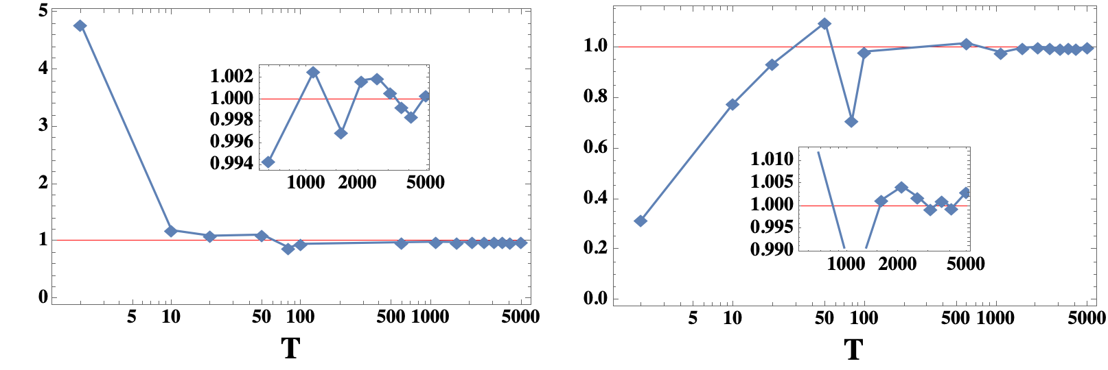
Figure 6: Time fluctuation of the integral in Eq.(28), $\frac{1}{T}\int^{T}_{0}dt{\rm Tr}\left[e^{iH_{D}t}\mathcal{P}_{D}^{\prime}e^{-iH_{D}t}{\bf J}_{\alpha}^{T}{\bf J}_{\alpha}\right]$ ($\alpha=\alpha_{1}$ for left panel and $\alpha=\alpha_{2}$ for right panel), as a function of $T$.

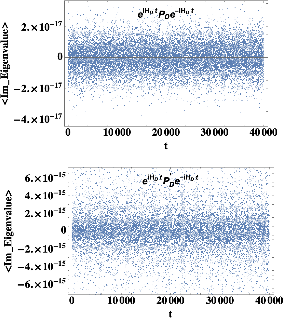
Figure 10: Time evolutions of the mean value of the imaginary part of eigenvalues for $e^{iH_{D}t}\mathcal{P}_{D}e^{-iH_{D}t}$ and $e^{iH_{D}t}\mathcal{P}^{\prime}_{D}e^{-iH_{D}t}$.

Note that although the Hermitian matrices $\mathcal{P}_{D}$ and $\mathcal{P}_{D}^{\prime}:=\sum_{j}|E_{j}\rangle\sum_{j}\langle E_{j}|$ have the same trace equal to $D$, they have different ranks, where the former is always full rank and be a identity matrix, while the latter is a rank-1 matrix. In terms of the quantum evolution, $e^{iH_{D}t}\mathcal{P}_{D}e^{-iH_{D}t}$ and $e^{iH_{D}t}\mathcal{P}_{D}^{\prime}e^{-iH_{D}t}$ are still the Hermitian matrices and their eigenvalues are independent of time, but we notice that they have quite different variances for the small imaginary part of eigenvalues which can be observed only in log scale, and also, their eigenvectors behave quite differently during the evolution of time. $e^{iH_{D}t}\mathcal{P}_{D}^{\prime}e^{-iH_{D}t}$ exhibits more significaant character in non-Hermiticity, that its eigenvectors keep mutually independent (do not forced to be mutually orthogonal and self-normalized with the evolution of time) while its imaginary parts of eigenvalues exhibit persistive level repulsion (in log scale) with the time evolution, which cannot be found in $e^{iH_{D}t}\mathcal{P}_{D}e^{-iH_{D}t}$. Further, as shown in Fig.10, for the mean value of the imaginary part of eigenvalues, $e^{iH_{D}t}\mathcal{P}_{D}^{\prime}e^{-iH_{D}t}$ exhibit larger fluctuation and a more mild approching to the zero axis.

In a word,$e^{iH_{D}t}\mathcal{P}_{D}e^{-iH_{D}t}$ exhibits many-body localization through the thermalization of integrable eigenstates, while such case of many-body localization can be shut off for $e^{iH_{D}t}\mathcal{P}_{D}^{\prime}e^{-iH_{D}t}$ as the product of two collection of eigenvectors (like $\sum_{j}|E_{j}\rangle$) do not exhibit relaxation to equilibrium in long-time limit. Thus the off-diagonal part contributes to the nonlocal symmetries within $e^{iH_{D}t}\mathcal{P}_{D}^{\prime}e^{-iH_{D}t}$. While for $e^{iH_{D}t}|\mathcal{J}_{\alpha_{1}}\rangle\langle\mathcal{J}_{\alpha_{1}}|e^{-iH_{D}t}$ or $e^{iH_{D}t}|\mathcal{J}_{\alpha_{2}}\rangle\langle\mathcal{J}_{\alpha_{2}}|e^{-iH_{D}t}$, there is also without the many-body localization as can be seem from the long-time behavior of eigenvector products (), but different to the case of $e^{iH_{D}t}\mathcal{P}_{D}^{\prime}e^{-iH_{D}t}$, the "level repulsion" (from Fig; which is not real level repulsion) does not contributed by the off-diagonal part which can also be evidenced by the absence of end response (or boundary correspondence in the evolution). Thus this should be classified into the case of strong disorder limit where the non-Hermicity is destoried and the off-diagonal part plays no role. Also, the Hermicity can be seem from the linearly increased variance as shown in Fig., which follows a fixed slope without any saturation (i.e., an extensive type accumulation insteda of scaling base on the corresponding expectations of each subsystem). One of the direct result of absence of saturation is the absence of level statistics.

Also, we found that $e^{iH_{D}t}\mathcal{P}_{D}^{\prime}{\bf J}^{T}_{\alpha}{\bf J}_{\alpha}e^{-iH_{D}t}$ or $e^{iH_{D}t}\mathcal{P}_{D}|\mathcal{J}_{\alpha}\rangle\langle\mathcal{J}_{\alpha}|e^{-iH_{D}t}$ behave in the same way with $e^{iH_{D}t}|\mathcal{J}_{\alpha}\rangle\langle\mathcal{J}_{\alpha}|e^{-iH_{D}t}$. Thus, except $\mathcal{P}_{D}^{\prime}$ and $|\mathcal{J}_{\alpha}\rangle\langle\mathcal{J}_{\alpha}|$, $\mathcal{P}_{D}^{\prime}{\bf J}^{T}_{\alpha}{\bf J}_{\alpha}$ and $\mathcal{P}_{D}\mathcal{J}_{\alpha}\rangle\langle\mathcal{J}_{\alpha}|$ can also be thermalized with respect to some certain observable.

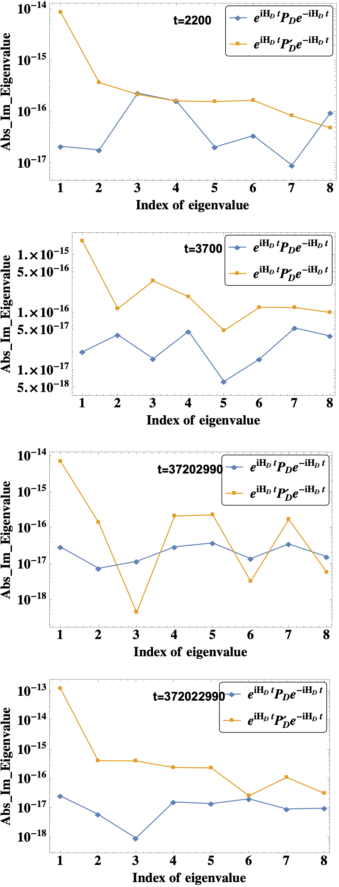
Figure 7: Absolute values of the imaginary part of eigenvalues of $e^{iH_{D}t}\mathcal{P}_{D}e^{-iH_{D}t}$ and $e^{iH_{D}t}\mathcal{P}^{\prime}_{D}e^{-iH_{D}t}$.

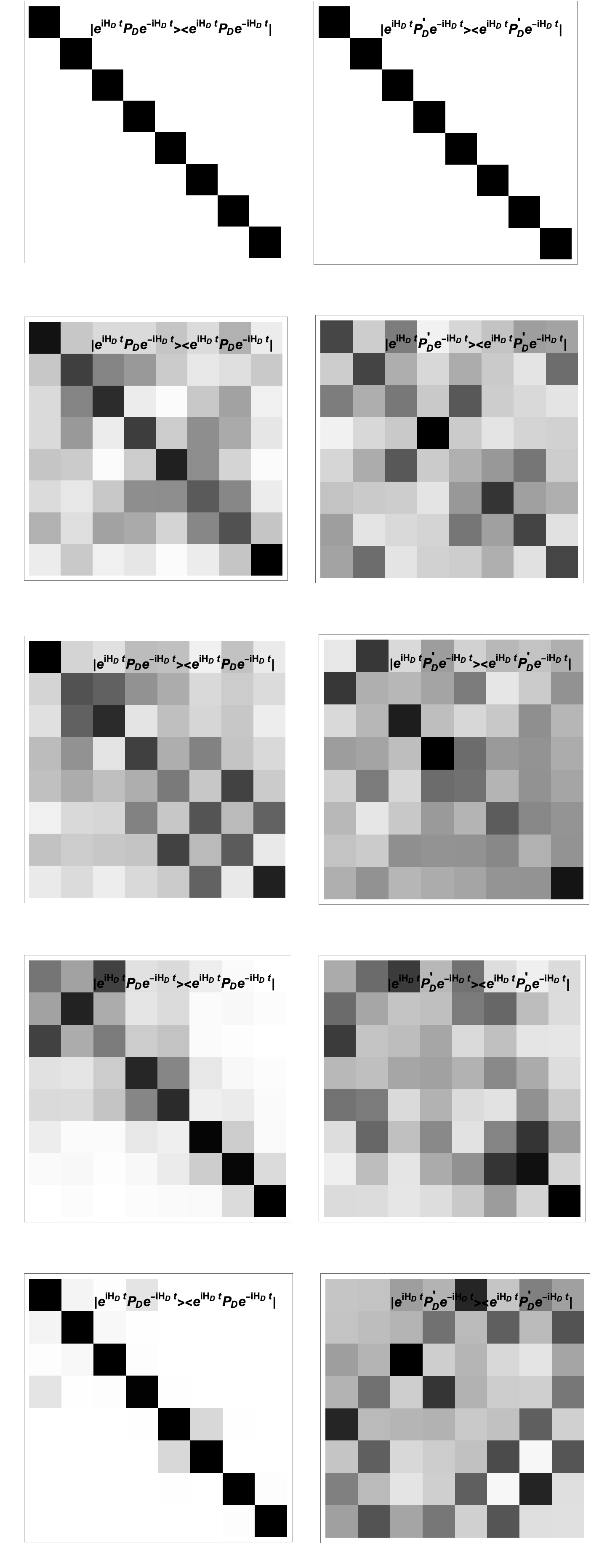
Figure 8: Matrix plots as the outer products between the eigenvectors of $e^{iH_{D}t}\mathcal{P}_{D}e^{-iH_{D}t}$ and that of $e^{iH_{D}t}\mathcal{P}^{\prime}_{D}e^{-iH_{D}t}$. The first to the last rows correspond to $t=0$, $t=0.8$, $t=50$, $t=150$, $t=3000$, respectively.

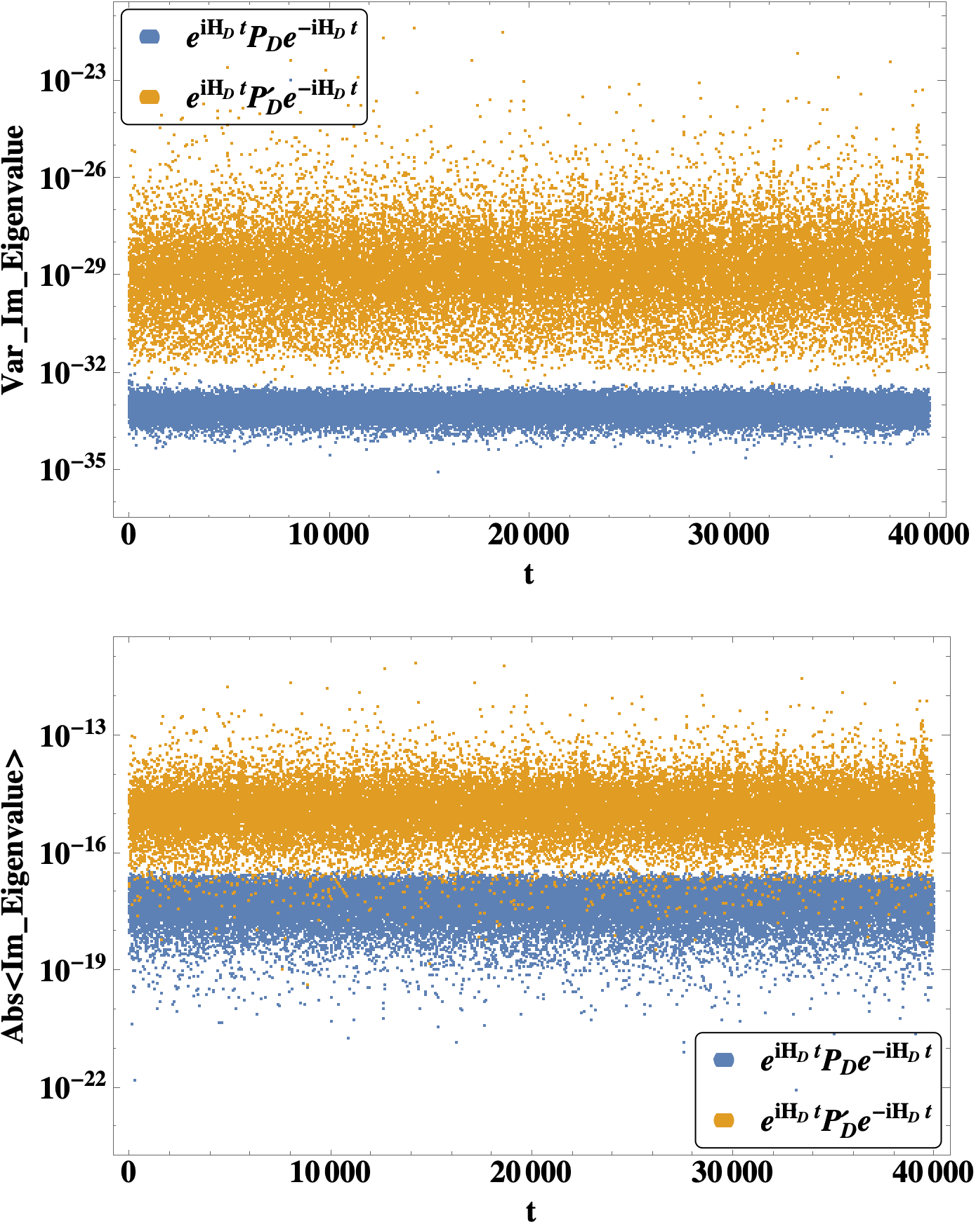
Figure 9: Time evolutions of the variance (top panel) and absolute value (bottom panel) of the mean value of the imaginary part of eigenvalues for $e^{iH_{D}t}\mathcal{P}_{D}e^{-iH_{D}t}$ and $e^{iH_{D}t}\mathcal{P}^{\prime}_{D}e^{-iH_{D}t}$. The non-Hermitian character can be seem from evolution of $e^{iH_{D}t}\mathcal{P}^{\prime}_{D}e^{-iH_{D}t}$ in the begining and end of the evolution. The difference between the begining and end of the evolution is enfored by the local conservations with level repulsion, as a necessary result of the non-Hermitian symmetry, while this cannot be found from $e^{iH_{D}t}\mathcal{P}_{D}e^{-iH_{D}t}$ which is nearly stable.

In other word, each diagonal element of $e^{iH_{D}t}\mathcal{P}_{D}e^{-iH_{D}t}$ can be thermalized with time evolution (as a consequence, its eigenvectors becomes mutually orthogonal and self-normalized in long-time limit) and as a result $e^{iH_{D}t}\mathcal{P}_{D}e^{-iH_{D}t}$ behaves more extensively as a Hermitian term; While each eigenvectors of $e^{iH_{D}t}\mathcal{P}_{D}^{\prime}e^{-iH_{D}t}$ exhibits insistent level repulsion and thus be mutually independent with the evolution of time, which leads to the absence of thermalization after the quench (i.e., adding two unitary operators to realizing the time evolution). The non-Hermitian feature of $e^{iH_{D}t}\mathcal{P}_{D}^{\prime}e^{-iH_{D}t}$ can also be found from its evolution by treating it as a whole observable, where the boundary-dependence can be seem from Fig.9 where, no matter how long the time evolution is, there is always be a sink in the begining and a bulge in the end (which is absent for $e^{iH_{D}t}\mathcal{P}_{D}e^{-iH_{D}t}$). Also, the persistive level repulsion for $e^{iH_{D}t}\mathcal{P}_{D}^{\prime}e^{-iH_{D}t}$ can be seem from the variance evolution, as it is the only explaination for the enhancement of variance (avoided accidental degeneration) after long-time evolution. Thus for $e^{iH_{D}t}\mathcal{P}_{D}^{\prime}e^{-iH_{D}t}$, the level repulsion exists between its replicas at different time.

As a consequence, $e^{iH_{D}t}\mathcal{P}_{D}^{\prime}e^{-iH_{D}t}$ as a (non-extensive) collection of initial states can be thermalized with respect to the observable ${\bf J}^{T}_{\alpha}{\bf J}_{\alpha}$. This is why the level repulsion can be observed only from the begining and end of the evolution. In other word, the localization for $e^{iH_{D}t}\mathcal{P}_{D}^{\prime}e^{-iH_{D}t}$ at a single time can be observed only begining and end of the spectrum (or variance of the mean values). Meanwhile, the unitary operator $e^{iH_{D}t}$ plays an important role in troducing the quenches away from the equilibrium.

Also, it should be distinguished from the above-discussed case, where the ${\bf\Psi}_{\alpha_{1}}$ keeps a non-defective degenerate region to guarantees the repulsion between degenerated levels, while the $e^{iH_{D}t}\mathcal{P}_{D}e^{-iH_{D}t}$ does not keeping the level repulsion even in log scale. In constrast, since $e^{iH_{D}t}\mathcal{P}_{D}^{\prime}e^{-iH_{D}t}$ withou the level repulsion and also without the non-defective character, there is only one (collective) observable that be able to thermalized with respect to ${\bf J}^{T}_{\alpha}{\bf J}_{\alpha}$, unlike the case for the ${\bf\Psi}_{\alpha_{1}}$ where its degenerated levels can be treated as thermalized with respect to itself as guaranteed by the robust diagonal correlation between the nondegenerated block (whose dimension tends to be 1 in many-subsystem limit) and the degenerated block. Note that in this case, the off-diagonal part for each subsystem does not form symmetry sector to guarantees the level repulsion and non-Hermicity.

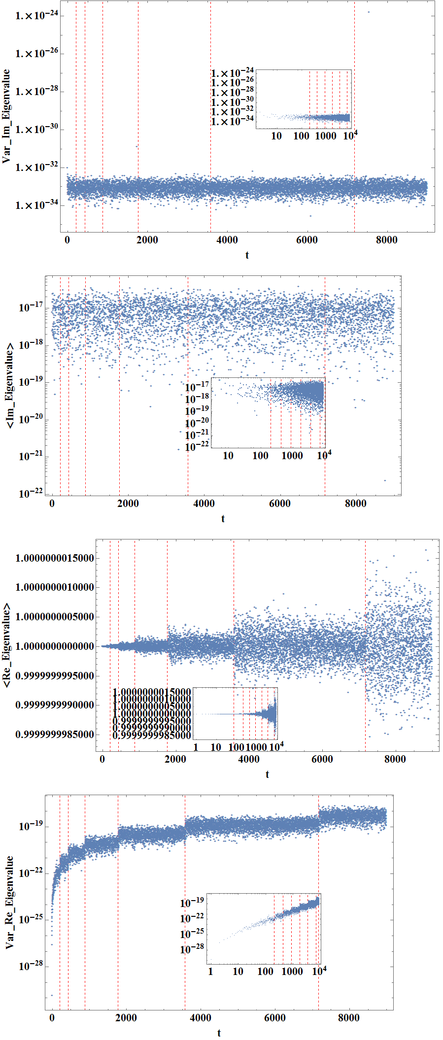
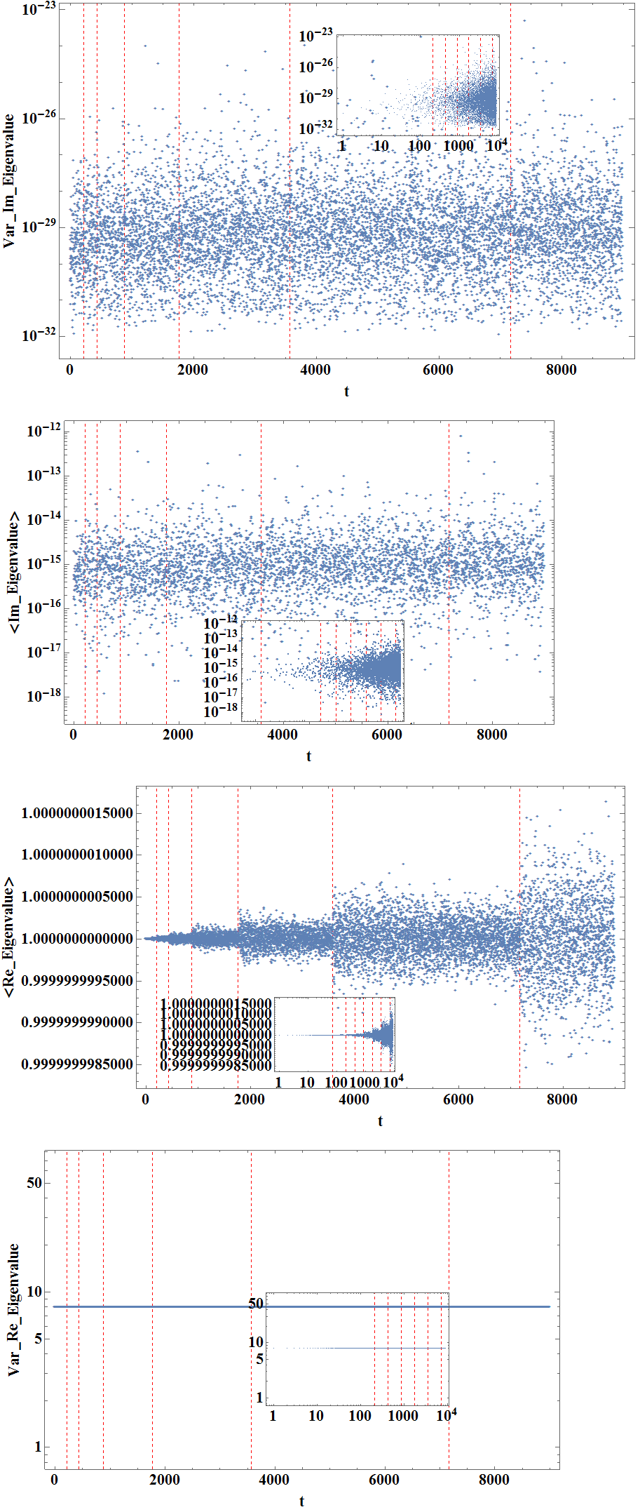
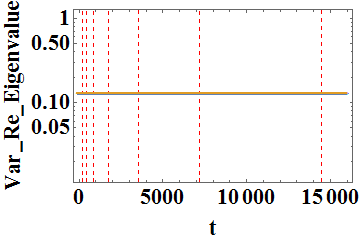
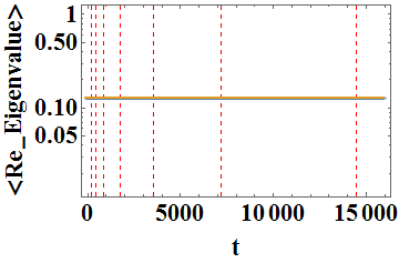
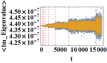
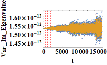
Figure 11: Time evolutions of the mean value and variance of the imaginary part and real part of eigenvalues for $e^{iH_{D}t}\mathcal{P}_{D}e^{-iH_{D}t}$. The imaginary part of eigenvalues exhibit no signal of thermalization or level repulsion From real part of eigenvalues, we can clearly see the quantization feature, i.e., the real part of spectrum evolved with time is consist of discontinuously connected segments where each one of them is governed by a non-Hermitian symmetry (as the edge burst can be seen from the left boundary of each segment; The red lines indicate the position of each edge burst: $t=208.772,434.43,875,1766,3572,7171.94$). Note that here the time interval for each segment does not increases in a fix ratio, but shift to larger ratio with the evolution. This means that there must be a edge at long-time limit, in which case the corresponding distincted levels correspond to the intervals of segments in ascending order. The pseudo-periodic reveals of thermalization for the real part of eigenvalues can be seen in terms of the mean value and variance for $\mathcal{P}_{D}$, while for $\mathcal{P}_{D}^{\prime}$ only that in terms of mean value preserve. As a result of stability of variance as shown in (), the correspondence to the above-mentioned edge at long-time limit can be overcomed by the fixed variance (as a nonlocal symmetry sector whose size is variant). Consequantly, the edge burst guaranteed by such nonlocal symmetry can be seen in imaginary spectrum () only for $\mathcal{P}_{D}^{\prime}$. In conclusion, the evolution of initial state of $\mathcal{P}_{D}^{\prime}$ is able to be non-Hermitian while that for $\mathcal{P}_{D}$ can only be a piece of spectrum of non-Hermitian system. In a sharp difference to the evolution of $e^{iH_{D}t}{\bf J}_{\alpha}^{T}{\bf J}_{\alpha}e^{-iH_{D}t}$, we reproduce the result of Fig.14(a) here in a larger scale. We found that, the imaginary spectrum of $e^{iH_{D}t}{\bf J}_{\alpha}^{T}{\bf J}_{\alpha}e^{-iH_{D}t}$ also exhibit quantization character but not as obvious as that for $\mathcal{P}_{D}$ and $\mathcal{P}_{D}^{\prime}$. This, again, explain the absence of level repulsion in Fig14(b).

6.2 Effect of multi-edge

The completely thermalization can be seem from Eq.(LABEL:10191), where the time evolution of $e^{-iH_{D}t}|\mathcal{J}_{\alpha}\rangle\langle\mathcal{J}_{\alpha}|e^{iH_{D}t}$ exhibits a simple linear increasing (without saturation) in the way of integrable state superposition. As a result, the final expectation for the thermalized state $e^{-iH_{D}t}|\mathcal{J}_{\alpha}\rangle\langle\mathcal{J}_{\alpha}|e^{iH_{D}t}$ with respect to ${\bf J}^{T}_{\alpha_{1}}{\bf J}_{\alpha_{1}}$ and ${\bf J}^{T}_{\alpha_{2}}{\bf J}_{\alpha_{2}}$ exhibit a obvious correlation ($3:1$ or $1:3$ as shown in Eq.(LABEL:10191)). In other word, in a system containing the initial state $|\mathcal{J}_{\alpha}\rangle\langle\mathcal{J}_{\alpha}|$, ${\bf J}^{T}_{\alpha}{\bf J}_{\alpha}$ provides the only "edge burst", i.e., the only source of the level repulsion between states $e^{-iH_{D}t}|\mathcal{J}_{\alpha}\rangle\langle\mathcal{J}_{\alpha}|e^{iH_{D}t}(t)$. That is why the traces in Eq.(LABEL:10191) reflect character of isolated system that completely decoupled with the environment. In contrast to this, there is already "edge burst" which can be seem from the evolution of $e^{-iH_{D}t}\mathcal{P}_{D}^{\prime}e^{iH_{D}t}$, as a result, we numerically obtain

$$\langle{\rm Tr}[{\bf J}^{T}_{\alpha_{2}}{\bf J}_{\alpha_{2}}]\rangle_{t}\gtrsim\langle{\rm Tr}[{\bf J}^{T}_{\alpha_{1}}{\bf J}_{\alpha_{1}}]\rangle_{t},$$ (29)

where

$$\langle{\rm Tr}[{\bf J}^{T}_{\alpha_{i}}{\bf J}_{\alpha_{i}}]\rangle_{t}:=\lim_{T\rightarrow\infty}\frac{1}{T}\int^{T}_{0}dt{\rm Tr}[e^{-iH_{D}t}\mathcal{P}_{D}^{\prime}e^{iH_{D}t}{\bf J}^{T}_{\alpha_{i}}{\bf J}_{\alpha_{i}}].$$ (30)

The reason is that ${\bf J}^{T}_{\alpha}{\bf J}_{\alpha}$ does not provides the only edge burst here, thus the resulting trace in Eq.(LABEL:) still have finite response to the "environment", and the level repulsion always exist between $\langle{\rm Tr}[{\bf J}^{T}_{\alpha_{i}}{\bf J}_{\alpha_{i}}]\rangle_{t}$'s.

Similar phenomenon can be observed from the evolution of initial states

$$\lim_{T\rightarrow\infty}\frac{1}{DT}\int^{T}_{0}dt{\rm Tr}[e^{-iH_{D}t}\sum_{i}|{\bf\Psi}_{\alpha_{1};i}\rangle\langle{\bf\Psi}_{\alpha_{1};i}^{*}|e^{iH_{D}t}{\bf J}^{T}_{\alpha_{1}}{\bf J}_{\alpha_{1}}]\lesssim\lim_{T\rightarrow\infty}\frac{1}{DT}\int^{T}_{0}dt{\rm Tr}[e^{-iH_{D}t}\sum_{i}|{\bf\Psi}_{\alpha_{1};i}\rangle\langle{\bf\Psi}_{\alpha_{1};i}^{*}|e^{iH_{D}t}{\bf J}^{T}_{\alpha_{2}}{\bf J}_{\alpha_{2}}]$$ (31)

$$\lesssim\lim_{T\rightarrow\infty}\frac{1}{DT}\int^{T}_{0}dt{\rm Tr}[e^{-iH_{D}t}\sum_{i}|{\bf\Psi}_{\alpha_{2};i}\rangle\langle{\bf\Psi}_{\alpha_{2};i}^{*}|e^{iH_{D}t}{\bf J}^{T}_{\alpha_{2}}{\bf J}_{\alpha_{2}}]\lesssim\lim_{T\rightarrow\infty}\frac{1}{DT}\int^{T}_{0}dt{\rm Tr}[e^{-iH_{D}t}\sum_{i}|{\bf\Psi}_{\alpha_{2};i}\rangle\langle{\bf\Psi}_{\alpha_{2};i}^{*}|e^{iH_{D}t}{\bf J}^{T}_{\alpha_{1}}{\bf J}_{\alpha_{1}}],$$

where according to our numerical result, each term in above expression converge to $0.12466,\ 0.12502,\ 0.1272,\ 0.1298$, respectively, at long time limit, where despite the minor fluctuations, there is always a fixed difference between them, which indicates the persistent level repulsion.

As the initial state need to be able to evolve according to a time-independent Hamiltonian, and localization (delocalization) of initial states directly determine the finial expectation with respect to the local-type observables ${\bf J}^{T}_{\alpha}{\bf J}_{\alpha}$. Such local-type observable can be called as non-destructive edge, as it does not eliminate the non-Hermicity of initial states. While the observables like ${\bf\Psi}_{\alpha}$, ${\bf J}^{H}_{\alpha}{\bf J}_{\alpha}$, and $|\mathcal{J}_{\alpha}\rangle\langle\mathcal{J}_{\alpha}|$ are destructive edges, which can be evidenced by the absence of level repulsion. Although such destructive edge can also leads to a relaxation to equilibrium state, but such relaxation is not completely originates from the level repulsion from original initial state without the edge. Thus the non-destructive edge must be: (1): not able to evolve according to the time-independent Hamiltonian $H_{D}$; (2): Without correlation with other observable. Here, the destructive observables ${\bf\Psi}_{\alpha}$ and $\mathcal{P}_{D}^{\prime}|\mathcal{J}_{\alpha}\rangle\langle\mathcal{J}_{\alpha}|$ violate the condition (2), while $\mathcal{P}_{D}^{\prime}{\bf J}_{\alpha}^{T}{\bf J}_{\alpha}$, ${\bf J}^{H}_{\alpha}{\bf J}_{\alpha}$, $\sum_{i}|{\bf\Psi}_{\alpha;i}\rangle\langle{\bf\Psi}_{\alpha;i}^{*}|$ and $|\mathcal{J}_{\alpha}\rangle\langle\mathcal{J}_{\alpha}|$ violate condition (1).

Another evidence for the level repulsion which exists for the non-Hermitian initial states and absent for Hermitian initial states is their evolution with respect to a observable. As a result, for initial state $\mathcal{P}_{D}$ which is Hermitian and cannot be thermalized, there is not the evolution for $e^{-iH_{D}t}\mathcal{P}_{D}e^{iH_{D}t}{\bf J}^{T}_{\alpha}{\bf J}_{\alpha}$; for initial state $\mathcal{P}_{D}^{\prime}$ which is non-Hermitian but cannot be completely thermalized with respect to ${\bf J}^{T}_{\alpha}{\bf J}_{\alpha}$, the evolution of $e^{-iH_{D}t}\mathcal{P}_{D}^{\prime}e^{iH_{D}t}{\bf J}^{T}_{\alpha}{\bf J}_{\alpha}$ exhibit level repulsion for $\alpha=1$ and $\alpha=2$; for initial state $|\mathcal{J}_{\alpha}\rangle\langle\mathcal{J}_{\alpha}|$ which is Hermitian and can be completely thermalized with respect to ${\bf J}^{T}_{\alpha}{\bf J}_{\alpha}$, the evolution of $e^{-iH_{D}t}|\mathcal{J}_{\alpha}\rangle\langle\mathcal{J}_{\alpha}|e^{iH_{D}t}{\bf J}^{T}_{\alpha}{\bf J}_{\alpha}$ exhibit no level repulsion. Importantly, the above-mentioned level repulsion only exist for the imaginary part of eigenvalues, which reflect a crucial dependence on the complex eigenvalue. It is also important to notice that the complex eigenfrequencies in a circuit have dramatical effects on the output signal resolution as well as the noise (frequencies). Further, the level repulsion disappear for initial state $\mathcal{P}_{D}^{\prime}$ with respect to $|\mathcal{J}_{\alpha}\rangle\langle\mathcal{J}_{\alpha}|$, ${\bf J}^{H}_{\alpha}{\bf J}_{\alpha}$, or ${\bf\Psi}_{\alpha}$, which means the level repulsion requires the observable does not contain non-defective degeneracies or other kinds of triggers for the correlations. In the mean time, this also indicates that the observable in some case does not have to be Hermitian (real eigenvalues), but just to be "local" enough, like the case we discuss here, where the observable ${\bf J}^{T}_{\alpha}{\bf J}_{\alpha}$ (despite the complex eigenvalue) behaves more locally than the Hermitian one ${\bf J}^{H}_{\alpha}{\bf J}_{\alpha}$ since there is higher degree of overlap between the eigenvalues of ${\bf J}^{T}_{\alpha_{1}}{\bf J}_{\alpha_{1}}$ and ${\bf J}^{T}_{\alpha_{2}}{\bf J}_{\alpha_{2}}$, compares to that between ${\bf J}^{H}_{\alpha_{1}}{\bf J}_{\alpha_{1}}$, and ${\bf J}^{H}_{\alpha_{2}}{\bf J}_{\alpha_{2}}$. In other word, level repulsion only appear between the evolutions (thermalization) of $\mathcal{P}_{D}^{\prime}$ with respect to two uncorrelated observables where each one of them behaves locally (due to the diagonal contribution), and such observable in this article should only be ${\bf J}_{\alpha}^{T}{\bf J}_{\alpha}$.

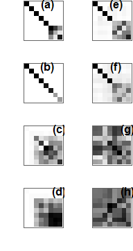
Figure 12: As an evidence for the localization of ${\bf J}^{T}_{\alpha}{\bf J}_{\alpha}$ and the delocalization of $|\mathcal{J}_{\alpha}\rangle\langle\mathcal{J}_{\alpha}|$. We show the eigenvector outer products of ${\bf J}^{T}_{\alpha_{1}}{\bf J}_{\alpha_{1}}$ ((a),(b)), ${\bf J}^{T}_{\alpha_{2}}{\bf J}_{\alpha_{2}}$ ((c),(d)), $|\mathcal{J}_{\alpha_{1}}\rangle\langle\mathcal{J}_{\alpha_{1}}|$ ((e),(f)), $|\mathcal{J}_{\alpha_{2}}\rangle\langle\mathcal{J}_{\alpha_{2}}|$ ((g),(h)), where the left column and right column correspond to zero time and long-time limit, respectively.

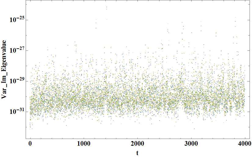
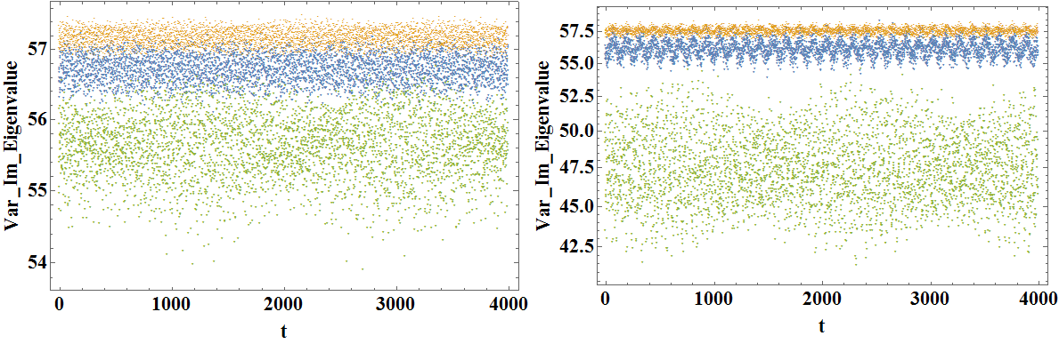
Figure 13: $e^{iH_{D}t}\sum_{i}|{\bf\Psi}_{\alpha;i}\rangle\langle{\bf\Psi}_{\alpha;i}^{*}|e^{-iH_{D}t}$ and $e^{iH_{D}t}\sum_{i}|{\bf\Psi}_{\alpha;i}\rangle\langle{\bf\Psi}_{\alpha;i}^{*}|e^{-iH_{D}t}{\bf J}^{T}_{\alpha_{1}}{\bf J}_{\alpha_{1}}$ for $\alpha=\alpha_{1}$ (blue), $\alpha=\alpha_{2}$ (orange), and $\alpha=\alpha_{3}$ (green).

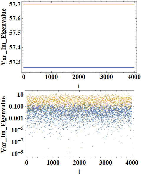
Figure 14: Evolution of $e^{iH_{D}t}{\bf J}_{\alpha}^{T}{\bf J}_{\alpha}e^{-iH_{D}t}$ (top panel) and $e^{iH_{D}t}\mathcal{P}_{D}^{\prime}e^{-iH_{D}t}{\bf J}_{\alpha}^{T}{\bf J}_{\alpha}$ (bottom panel) with $\alpha=\alpha_{1}$ (blue) and $\alpha=\alpha_{2}$ (orange).

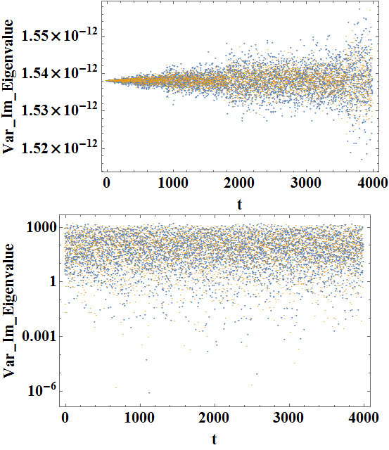
Figure 15: Evolution of $e^{iH_{D}t}|\mathcal{J}_{\alpha}\rangle\langle\mathcal{J}_{\alpha}|e^{-iH_{D}t}$ (top panel) and $e^{iH_{D}t}\mathcal{P}_{D}^{\prime}e^{-iH_{D}t}|\mathcal{J}_{\alpha}\rangle\langle\mathcal{J}_{\alpha}|$ (bottom panel) with $\alpha=\alpha_{1}$ (blue) and $\alpha=\alpha_{2}$ (orange).

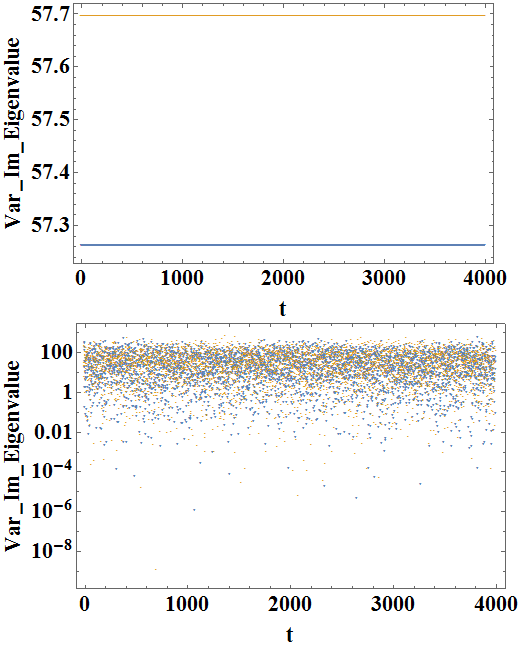
Figure 16: Evolution of $e^{iH_{D}t}{\bf\Psi}_{\alpha}e^{-iH_{D}t}$ (top panel) and $e^{iH_{D}t}\mathcal{P}_{D}^{\prime}e^{-iH_{D}t}{\bf\Psi}_{\alpha}$ (bottom panel) with $\alpha=\alpha_{1}$ (blue) and $\alpha=\alpha_{2}$ (orange).

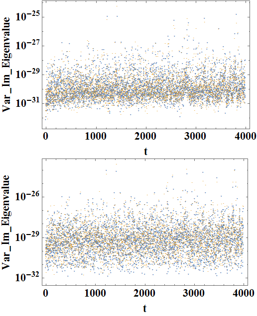
Figure 17: Evolution of $e^{iH_{D}t}\sum_{i}|{\bf\Psi}_{\alpha;i}\rangle\langle{\bf\Psi}_{\alpha;i}^{*}|e^{-iH_{D}t}$ (top panel) and $e^{iH_{D}t}\mathcal{P}_{D}^{\prime}e^{-iH_{D}t}\sum_{i}|{\bf\Psi}_{\alpha;i}\rangle\langle{\bf\Psi}_{\alpha;i}^{*}|$ (bottom panel) with $\alpha=\alpha_{1}$ (blue) and $\alpha=\alpha_{2}$ (orange). In contrast to the observable ${\bf J}_{\alpha}^{T}{\bf J}_{\alpha}$ the level repulsion between different observable is being replaced by that between different $t$.

6.3 Hilbert–Schmidt product

In terms of projector $\mathcal{P}_{D}$ (onto the size-dependent sector Hamiltonian $H_{D}$) with normalized basis ($\langle E_{j}|E_{j^{\prime}}\rangle=\delta_{jj^{\prime}},\ \sum_{j}\langle E_{j}|E_{j}\rangle=D$), we can rewrite the above expression in the form of microcanonical ensemble average,

$${\rm Tr}[{\bf J}_{\alpha}^{T}{\bf J}_{\alpha}] ={\rm Tr}\left[e^{iH_{D}t}\mathcal{P}_{D}{\bf J}_{\alpha}^{T}{\bf J}_{\alpha}e^{-iH_{D}t}\right]$$ (32)

$$={\rm Tr}\left[e^{iH_{D}t}{\bf J}_{\alpha}^{T}{\bf J}_{\alpha}\mathcal{P}_{D}e^{-iH_{D}t}\right]$$

$$={\rm Tr}\left[e^{iH_{D}t}\mathcal{P}_{D}e^{-iH_{D}t}{\bf J}_{\alpha}^{T}{\bf J}_{\alpha}\right]$$

$$={\rm Tr}\left[{\bf J}_{\alpha}^{T}{\bf J}_{\alpha}e^{iH_{D}t}\mathcal{P}_{D}e^{-iH_{D}t}\right]$$

where $[\mathcal{P}_{D},{\bf J}_{\alpha}^{T}{\bf J}_{\alpha}]=0,\ [e^{iH_{D}t}\mathcal{P}_{D}e^{-iH_{D}t},{\bf J}_{\alpha}^{T}{\bf J}_{\alpha}]=0$. Here $\intercal_{\alpha;1}:=e^{iH_{D}t}{\bf J}_{\alpha}^{T}{\bf J}_{\alpha}\mathcal{P}_{D}e^{-iH_{D}t}$ and $\intercal_{\alpha;2}:={\bf J}_{\alpha}^{T}{\bf J}_{\alpha}e^{iH_{D}t}\mathcal{P}_{D}e^{-iH_{D}t}$ are a pair of similar matrix with rank larger than one and conserved trace (${\rm Tr}\intercal_{\alpha;1}={\rm Tr}\intercal_{\alpha;2}=1$), and they have the same singular values which are independent of time. Indeed, we have verified that $\intercal_{\alpha;2}$ is the Hilbert-Schmidt operator (Endomorphism) while $\intercal_{\alpha;1}$ is not although it share the same Hilbert-Schmidt norm in some cases:

$$||\intercal_{\alpha;1}||_{HS}=||\sqrt{\intercal_{\alpha;1}^{{\dagger}}\intercal_{\alpha;1}}||_{HS}=||\sqrt{\intercal_{\alpha;1}\intercal_{\alpha;1}^{{\dagger}}}||_{HS}=\sqrt{{\rm Tr}[\intercal_{\alpha;1}^{{\dagger}}\intercal_{\alpha;1}]}=\sqrt{{\rm Tr}[\intercal_{\alpha;1}\intercal_{\alpha;1}^{{\dagger}}]}$$ (33)

$$=||\intercal_{\alpha;2}||_{HS}=||{\bf J}^{T}_{\alpha}{\bf J}_{\alpha}||_{HS}=||\sqrt{\intercal_{\alpha;2}^{*}\intercal_{\alpha;2}}||_{HS}=||\sqrt{\intercal_{\alpha;2}\intercal_{\alpha;2}^{*}}||_{HS}=\sqrt{{\rm Tr}[\intercal_{\alpha;2}^{*}\intercal_{\alpha;2}]}=\sqrt{{\rm Tr}[\intercal_{\alpha;2}\intercal_{\alpha;2}^{*}]}$$

$$={\rm Tr}[\sqrt{\intercal_{\alpha;1}^{{\dagger}}\intercal_{\alpha;1}}]+o(1)={\rm Tr}[\sqrt{\intercal_{\alpha;2}^{*}\intercal_{\alpha;2}}]+o(1),$$

$${\rm Tr}[\sqrt{\intercal_{\alpha;1}^{{\dagger}}\intercal_{\alpha;1}}]={\rm Tr}[\sqrt{\intercal_{\alpha;1}\intercal_{\alpha;1}^{{\dagger}}}]={\rm Tr}[\sqrt{\intercal_{\alpha;2}^{*}\intercal_{\alpha;2}}]={\rm Tr}[\sqrt{\intercal_{\alpha;2}\intercal_{\alpha;2}^{*}}]\neq{\rm Tr}[\sqrt{\intercal_{\alpha;1}^{*}\intercal_{\alpha;1}}]={\rm Tr}[\sqrt{\intercal_{\alpha;1}\intercal_{\alpha;1}^{*}}],$$

whose values depends only on the subscript $\alpha$ insteds of time $t$. $\intercal_{\alpha;1}$ and $\intercal_{\alpha;2}$ share the same (normalized) trace, and ${\rm Tr}[\intercal_{\alpha;1}^{r}]={\rm Tr}[\intercal_{\alpha;2}^{r}]$ be independent of $t$, where the superscript $r$ denotes the matrix power. Since $\intercal_{\alpha;1}$ and $\intercal_{\alpha;2}$ are similar, they share the same linear map, and in the case that $\intercal_{\alpha;1}$ and $\intercal_{\alpha;2}$ are all full rank, they are bijective.

While for $|\intercal_{\alpha;1}|$ and $|\intercal_{\alpha;2}|$, which means replacing all the entrices by its absolute value, ${\rm Tr}[|\intercal_{\alpha;2}|^{r}]$ are $t$-independent, but ${\rm Tr}[|\intercal_{\alpha;1}|^{r}]$ is $t$-dependent. The key reason for this difference is that the $\intercal_{\alpha;2}$ is symmetry ($\intercal_{\alpha;2}^{{\dagger}}=\intercal_{\alpha;2}^{*}$) while $\intercal_{\alpha;1}$ is not for $t\neq 0$. Due to this reason, we also have

$${\rm Re}[\intercal_{\alpha;2}^{2}]={\rm Re}[(\intercal_{\alpha;2}^{*})^{2}],{\rm Im}[\intercal_{\alpha;2}^{2}]=-{\rm Im}[(\intercal_{\alpha;2}^{*})^{2}],{\rm Re}[\intercal_{\alpha;2}\intercal_{\alpha;2}^{*}]={\rm Re}[\intercal_{\alpha;2}^{*}\intercal_{\alpha;2}],{\rm Im}[\intercal_{\alpha;2}\intercal_{\alpha;2}^{*}]=-{\rm Im}[\intercal_{\alpha;2}^{*}\intercal_{\alpha;2}],$$ (34)

$${\rm Tr}[|\intercal_{\alpha;2}|^{2}]={\rm Tr}[\intercal_{\alpha;2}\intercal_{\alpha;2}^{*}]={\rm Tr}[\intercal_{\alpha;2}^{*}\intercal_{\alpha;2}]={\rm Tr}[\intercal_{\alpha;1}\intercal_{\alpha;1}^{{\dagger}}]={\rm Tr}[\intercal_{\alpha;1}^{{\dagger}}\intercal_{\alpha;1}],$$

where the matrices in second line are all positive-defined. Also, the matrices $|\intercal_{\alpha;2}|^{2}$, $\intercal_{\alpha;2}\intercal_{\alpha;2}^{*}$, and $\intercal_{\alpha;2}^{*}\intercal_{\alpha;2}$ share the same (real) diagonal elements. According to the property of Hilbert–Schmidt operator, the complex and symmetry matrix $\intercal_{\alpha;2}$ corresponds to a linear endomorphism. From Eq.(LABEL:9101), the unitary dynamic with local measurements can be seem from $||\intercal_{\alpha;2}\mho||_{HS}=\sqrt{{\rm Tr}[\intercal_{\alpha;2}\intercal_{\alpha;2}^{*}]}$, where $\mho$ is arbitary unitary matrix. While the nonunitary dynamics can be seem from the time-dependence of the non-positive-defined matrices $\intercal_{\alpha;1}\intercal_{\alpha;1}^{*}$ or $\intercal_{\alpha;1}^{*}\intercal_{\alpha;1}$ governed by an effective non-Hermitian Hamiltonian.

For a bipartite system where we consider $\alpha_{1}\notin\underline{\alpha}$, $\alpha_{2}\in\underline{\alpha}$,

$$\langle{\rm Tr}[\intercal_{\alpha;1}\intercal_{\alpha;1}^{*}]\rangle_{t}:=\lim_{T\rightarrow\infty}\frac{1}{T}\int^{T}_{0}dt{\rm Tr}[\intercal_{\alpha_{1};1}\intercal_{\alpha_{1};1}^{*}]=\lim_{T\rightarrow\infty}\frac{1}{T}\int^{T}_{0}dt{\rm Tr}[\intercal_{\alpha_{2};1}\intercal_{\alpha_{2};1}^{*}]={\rm Tr}[\intercal_{\alpha;2}\intercal_{\alpha;2}^{*}]+o(1),$$ (35)

$${\rm Tr}[\intercal_{\alpha_{1};1}\intercal_{\alpha_{2};1}^{*}]={\rm Tr}[\intercal_{\alpha_{2};1}\intercal_{\alpha_{1};1}^{*}],$$

$$\lim_{T\rightarrow\infty}\frac{1}{T}\int^{T}_{0}dt{\rm Tr}[\intercal_{\alpha_{1};1}\intercal_{\alpha_{2};1}^{*}]=\frac{1}{D}.$$

Here ${\rm Tr}[\intercal_{\alpha;2}\intercal_{\alpha;2}^{*}]$ is independent of time, and has close values for $\alpha_{1}$ and $\alpha_{2}$

$${\rm Tr}[\intercal_{\alpha;2}\intercal_{\alpha;2}^{*}]={\rm Tr}[{\bf J}_{\alpha}^{T}{\bf J}_{\alpha}({\bf J}_{\alpha}^{T}{\bf J}_{\alpha})^{*}],$$ (36)

$$\frac{{\rm Tr}[\intercal_{\alpha_{1};2}\intercal_{\alpha_{1};2}^{*}]+{\rm Tr}[\intercal_{\alpha_{2};2}\intercal_{\alpha_{2};2}^{*}]}{2}\approx\frac{2}{D}{\rm Tr}[|\mathcal{J}_{\alpha}\rangle\langle\mathcal{J}_{\alpha}|],$$

$${\rm Tr}[|\mathcal{J}_{\alpha_{1}}\rangle\langle\mathcal{J}_{\alpha_{1}}|(|\mathcal{J}_{\alpha_{1}}\rangle\langle\mathcal{J}_{\alpha_{1}}|)^{*}]={\rm Tr}[|\mathcal{J}_{\alpha_{2}}\rangle\langle\mathcal{J}_{\alpha_{2}}|(|\mathcal{J}_{\alpha_{2}}\rangle\langle\mathcal{J}_{\alpha_{2}}|)^{*}],$$

$$\frac{||\intercal_{\alpha_{1};2}||_{HS}+||\intercal_{\alpha_{2};2}||_{HS}}{2}\approx\frac{1}{2}|||\mathcal{J}_{\alpha}\rangle\langle\mathcal{J}_{\alpha}|||_{HS},$$

where the outer product of the initial basis of diagonal ensemble $\{|\mathcal{J}_{\alpha}\rangle\}$ emphasize the ergodicity over the $\alpha_{1}$ and $\alpha_{2}$.

Moreover,

$$D{\rm Tr}[\rho_{\alpha}{\bf J}_{\alpha}^{T}{\bf J}_{\alpha}(\rho_{\alpha}{\bf J}_{\alpha}^{T}{\bf J}_{\alpha})^{*}]\approx\frac{\langle{\rm Tr}[\intercal_{\alpha;1}\intercal_{\alpha;1}^{*}]\rangle_{t}+{\rm Tr}[\intercal_{\alpha_{2};2}\intercal_{\alpha_{2};2}^{*}]}{2},$$ (37)

$$\frac{{\rm Tr}[\rho_{\alpha}{\bf J}_{\alpha}^{T}{\bf J}_{\alpha}(\rho_{\alpha}{\bf J}_{\alpha}^{T}{\bf J}_{\alpha})^{H}]}{\langle{\rm Tr}[\intercal_{\alpha;1}\intercal_{\alpha;1}^{*}]\rangle_{t}}={\rm Tr}[\intercal_{\alpha_{2};2}\intercal_{\alpha_{2};2}^{*}],$$

$$\frac{{\rm Tr}[\rho_{\alpha}{\bf J}_{\alpha}^{T}{\bf J}_{\alpha}(\rho_{\alpha}{\bf J}_{\alpha}^{T}{\bf J}_{\alpha})^{H}]}{{\rm Tr}[\rho_{\alpha}{\bf J}_{\alpha}^{T}{\bf J}_{\alpha}(\rho_{\alpha}{\bf J}_{\alpha}^{T}{\bf J}_{\alpha})^{*}]}\approx\frac{1}{2}D({\rm Tr}[\intercal_{\alpha_{2};2}\intercal_{\alpha_{2};2}^{*}]+\langle{\rm Tr}[\intercal_{\alpha;1}\intercal_{\alpha;1}^{*}]\rangle_{t}).$$

Although the symmetry complex matrix $\intercal_{\alpha;2}$ cannot be a Hermitian or non-Hermitian matrix by itself, it is closely related to the Hermiticity as well as the unitary dynamics of the bipartite system. This can be seem through the Takagi decomposition, $\intercal_{\alpha;2}=\mho_{1}\Lambda\mho_{1}^{T}$ where $\Lambda$ is the diagonal matrix whose diagonal elements are the singular values of $\intercal_{\alpha;2}$, $\mho_{1}=\mho_{2}\sqrt{\mho_{2}^{H}\nu_{2}^{*}}$ with $\mho_{2}$ and $\nu_{2}$ the matrices whose columns are the left- and right-singular vectors of $\intercal_{\alpha;2}$, respectively.

In terms of the normal matrix $(\intercal_{\alpha;2}+i\intercal_{\alpha;2}^{*})$,

$${\rm Tr}[\intercal_{\alpha;2}\intercal_{\alpha;2}^{*}]=\frac{1}{4}{\rm Tr}[(\intercal_{\alpha;2}+i\intercal_{\alpha;2}^{*})(\intercal_{\alpha;2}+i\intercal_{\alpha;2}^{*})^{*}+(\intercal_{\alpha;2}-i\intercal_{\alpha;2}^{*})(\intercal_{\alpha;2}-i\intercal_{\alpha;2}^{*})^{*}],$$ (38)

$${\rm Re}[{\rm Tr}[(\intercal_{\alpha;2}+i\intercal_{\alpha;2}^{*})(\intercal_{\alpha;2}-i\intercal_{\alpha;2}^{*})^{*}]]={\rm Re}[{\rm Tr}[(\intercal_{\alpha;2}+i\intercal_{\alpha;2}^{*})^{*}(\intercal_{\alpha;2}-i\intercal_{\alpha;2}^{*})]]=0,$$

where the last line is due to ${\rm Re}[i\intercal_{\alpha;2}\intercal_{\alpha;2}^{*}]=-{\rm Re}[i\intercal_{\alpha;2}^{*}\intercal_{\alpha;2}],{\rm Im}[i\intercal_{\alpha;2}\intercal_{\alpha;2}^{*}]={\rm Im}[i\intercal_{\alpha;2}^{*}\intercal_{\alpha;2}]$. Thus, as far as there is a singule sector with Hilbert space dimension $D$, the time-dependent projectors (or the orthogonal basis) perform a trace-preserving mapping which indicating a single sector. While the original projector $\mathcal{P}_{D}$ multipled by ${\bf J}_{\alpha}^{T}{\bf J}_{\alpha}$ on its left or right, the projector performs nomore the trace conserving mapping, and this process is equivalents to an estimation of expectation of ${\bf J}_{\alpha}^{T}{\bf J}_{\alpha}$ in the biorthogonal basis as shown in the last two lines of Eq.(28).

6.4 $\rho_{\alpha}{\bf J}_{\alpha}^{T}{\bf J}_{\alpha}$

While ${\bf J}_{\alpha}^{T}{\bf J}_{\alpha}e^{iH_{D}t}\sum_{j}|E_{j}\rangle\sum_{j}\langle E_{j}|e^{-iH_{D}t}$ and $e^{iH_{D}t}\sum_{j}|E_{j}\rangle\sum_{j}\langle E_{j}|e^{-iH_{D}t}{\bf J}_{\alpha}^{T}{\bf J}_{\alpha}$ are a pair of similar matrix that are both rank-1. Consequently, their corresponding unique singular values are guaranteed to be the same only at $t=0$.

In Eq.(3), we can further introduce a vector $|\mathcal{J}_{\alpha}\rangle$ which is able play the same role as ${\bf J}_{\alpha}^{T}$,

$$\langle E_{j}|{\bf J}^{T}_{\alpha}{\bf J}_{\alpha}|E_{j}\rangle=\langle E_{j}|\mathcal{J}_{\alpha}\rangle\langle\mathcal{J}_{\alpha}|E_{j}\rangle,\ \forall j,$$ (39)

which can be normalized as

$$\sum_{j}|\langle E_{j}|\mathcal{J}_{\alpha}\rangle|^{2}=\langle\mathcal{J}_{\alpha}|\mathcal{P}_{D}|\mathcal{J}_{\alpha}\rangle=\sum_{j}\langle E_{j}|{\bf J}^{T}_{\alpha}{\bf J}_{\alpha}|E_{j}\rangle=\sum_{j}\langle E_{j}|{\bf J}_{\alpha}{\bf J}^{T}_{\alpha}|E_{j}\rangle=\sum_{j}\langle E_{j}|\mathcal{J}_{\alpha}\rangle\langle\mathcal{J}_{\alpha}|E_{j}\rangle$$ (40)

$$={\rm Tr}[\boldsymbol{\mathcal{E}}|\mathcal{J}_{\alpha}\rangle\langle\mathcal{J}_{\alpha}|\boldsymbol{\mathcal{E}}^{T}]={\rm Tr}[\boldsymbol{\mathcal{E}}|{\bf J}_{\alpha}{\bf J}^{T}_{\alpha}|\boldsymbol{\mathcal{E}}^{T}]=1,$$

$${\rm Rank}[|\mathcal{J}_{\alpha}\rangle\langle\mathcal{J}_{\alpha}|]={\rm Tr}[|\mathcal{J}_{\alpha}\rangle\langle\mathcal{J}_{\alpha}|]={\rm Tr}[{\bf J}_{\alpha}^{T}{\bf J}_{\alpha}]=\langle\mathcal{J}_{\alpha}|\mathcal{J}_{\alpha}\rangle=1,\ \forall\alpha,$$

$${\rm Rank}[\sum_{\alpha}^{\alpha_{m}}|\mathcal{J}_{\alpha}\rangle\langle\mathcal{J}_{\alpha}|]={\rm Tr}[\sum_{\alpha}^{\alpha_{m}}|\mathcal{J}_{\alpha}\rangle\langle\mathcal{J}_{\alpha}|]=\alpha_{m},$$

where $\boldsymbol{\mathcal{E}}$ is the matrix whose rows are the eigenvectors of $H_{j}$, $\langle E_{j}|$. $\overline{\langle E_{j}|\mathcal{J}_{\alpha_{1}}\rangle}=\overline{\langle E_{j}|\mathcal{J}_{\alpha_{2}}\rangle}=\frac{1}{D}$. Then in terms of the diagonal ensemble for the macroscopic observable ${\bf J}^{T}_{\alpha}{\bf J}_{\alpha}$,

$${\rm Tr}[\rho_{\alpha}{\bf J}^{T}_{\alpha}{\bf J}_{\alpha}]={\rm Tr}[\rho_{\alpha}(t){\bf J}^{T}_{\alpha}{\bf J}_{\alpha}]={\rm Tr}[|\mathcal{J}_{\alpha}(t)\rangle\langle\mathcal{J}_{\alpha}(t)|\rho_{\alpha}]$$ (41)

$$=\langle\mathcal{J}_{\alpha}|\rho_{\alpha}|\mathcal{J}_{\alpha}\rangle=\langle\mathcal{J}_{\alpha}(t)|\rho_{\alpha}|\mathcal{J}_{\alpha}(t)\rangle\ (\forall t)$$

$$=\sum_{j}\langle E_{j}|e^{iE_{j}t}\langle\mathcal{J}_{\alpha}|E_{j}\rangle|\langle E_{j}|\mathcal{J}_{\alpha}\rangle|^{2}|E_{j}\rangle\langle E_{j}|\langle E_{j}|\mathcal{J}_{\alpha}\rangle e^{-iE_{j}t}|E_{j}\rangle$$

$$=\lim_{T\rightarrow\infty}\frac{1}{T}\int^{T}_{0}dt\langle\mathcal{J}_{\alpha}(t)|{\bf J}^{T}_{\alpha}{\bf J}_{\alpha}|\mathcal{J}_{\alpha}(t)\rangle$$

$$=\lim_{T\rightarrow\infty}\frac{1}{T}\int^{T}_{0}dt{\rm Tr}[|\mathcal{J}_{\alpha}(t)\rangle\langle\mathcal{J}_{\alpha}(t)|{\bf J}^{T}_{\alpha}{\bf J}_{\alpha}]$$

$$=\sum_{j}|\langle E_{j}|\mathcal{J}_{\alpha}\rangle|^{2}\langle{\bf J}^{T}_{\alpha}{\bf J}_{\alpha}\rangle_{mc}+o(1),$$

$$\rho_{\alpha}=\sum_{j}|\langle E_{j}|\mathcal{J}_{\alpha}\rangle|^{2}|E_{j}\rangle\langle E_{j}|=\sum_{j}\langle E_{j}|\mathcal{J}_{\alpha}\rangle|E_{j}\rangle\langle E_{j}|\langle\mathcal{J}_{\alpha}|E_{j}\rangle,$$

$$\left(=e^{iH_{D}t}\sum_{j}|\langle E_{j}|\mathcal{J}_{\alpha}\rangle|^{2}|E_{j}\rangle\langle E_{j}|e^{-iH_{D}t}=\sum_{j}\langle E_{j}|\mathcal{J}_{\alpha}\rangle e^{iE_{j}t}|E_{j}\rangle\langle E_{j}|e^{-iE_{j}t}\langle\mathcal{J}_{\alpha}|E_{j}\rangle\right)$$

$$\rho_{\alpha}(t)\mathcal{O}:=e^{iH_{D}t}\rho_{\alpha}\mathcal{O}e^{-iH_{D}t},$$

$$|\mathcal{J}_{\alpha}(t)\rangle=\sum_{j}\langle E_{j}|\mathcal{J}_{\alpha}\rangle e^{-iE_{j}t}|E_{j}\rangle=\sum_{j}\langle E_{j}|\mathcal{J}_{\alpha}\rangle e^{-iH_{D}t}|E_{j}\rangle,$$

where $\rho_{\alpha}$ (${\rm Tr}\rho_{\alpha}=1,\ {\rm Rank}\rho_{\alpha}=D$) is the stationary density matrix (microcanonical ensemble) of the diagonal ensemble.

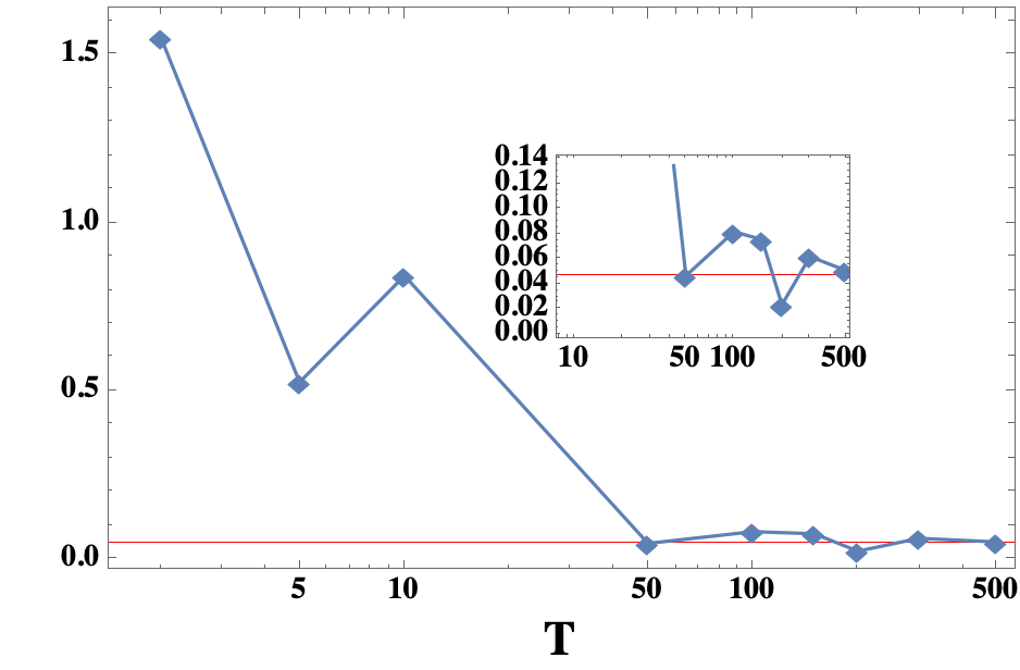
Figure 18: Time fluctuation of the integral in Eq.(LABEL:8231), $\frac{1}{DT}\int^{T}_{0}dt{\rm Tr}[|\mathcal{J}_{\alpha}(t)\rangle\langle\mathcal{J}_{\alpha}(t)|{\bf J}^{T}_{\alpha}{\bf J}_{\alpha}]$ as a function of $T$. The red line indicates the approaching tp $\frac{3}{D^{2}}=0.046875$.

For bipartite system, we found that

$${\rm Tr}[\sum_{j}|\langle E_{j}|\mathcal{J}_{\alpha_{1}}\rangle|^{2}|E_{j}\rangle\langle E_{j}|\langle{\bf J}^{T}_{\alpha_{1}}{\bf J}_{\alpha_{1}}]={\rm Tr}[\sum_{j}|\langle E_{j}|\mathcal{J}_{\alpha_{2}}\rangle|^{2}|E_{j}\rangle\langle E_{j}|\langle{\bf J}^{T}_{\alpha_{2}}{\bf J}_{\alpha_{2}}]$$ (42)

$$=\lim_{T\rightarrow\infty}\frac{1}{T}\int^{T}_{0}dt{\rm Tr}[|\mathcal{J}_{\alpha_{1}}(t)\rangle\langle\mathcal{J}_{\alpha_{1}}(t)|{\bf J}^{T}_{\alpha_{1}}{\bf J}_{\alpha_{1}}]$$

$$=\lim_{T\rightarrow\infty}\frac{1}{T}\int^{T}_{0}dt{\rm Tr}[|\mathcal{J}_{\alpha_{2}}(t)\rangle\langle\mathcal{J}_{\alpha_{2}}(t)|{\bf J}^{T}_{\alpha_{2}}{\bf J}_{\alpha_{2}}]=\frac{3}{D^{2}},$$

$${\rm Tr}[\sum_{j}|\langle E_{j}|\mathcal{J}_{\alpha_{1}}\rangle|^{2}|E_{j}\rangle\langle E_{j}|\langle{\bf J}^{T}_{\alpha_{2}}{\bf J}_{\alpha_{2}}]={\rm Tr}[\sum_{j}|\langle E_{j}|\mathcal{J}_{\alpha_{2}}\rangle|^{2}|E_{j}\rangle\langle E_{j}|\langle{\bf J}^{T}_{\alpha_{1}}{\bf J}_{\alpha_{1}}]$$

$$=\lim_{T\rightarrow\infty}\frac{1}{T}\int^{T}_{0}dt{\rm Tr}[|\mathcal{J}_{\alpha_{1}}(t)\rangle\langle\mathcal{J}_{\alpha_{1}}(t)|{\bf J}^{T}_{\alpha_{2}}{\bf J}_{\alpha_{2}}]$$

$$=\lim_{T\rightarrow\infty}\frac{1}{T}\int^{T}_{0}dt{\rm Tr}[|\mathcal{J}_{\alpha_{2}}(t)\rangle\langle\mathcal{J}_{\alpha_{2}}(t)|{\bf J}^{T}_{\alpha_{1}}{\bf J}_{\alpha_{1}}]=\frac{1}{D^{2}},$$

$${\rm Tr}[|\mathcal{J}_{\alpha}\rangle\langle\mathcal{J}_{\alpha}|]={\rm Tr}[|\mathcal{J}_{\alpha}(t)\rangle\langle\mathcal{J}_{\alpha}(t)|]$$ (43)

$$={\rm Tr}[\sum_{j}\langle E_{j}|\mathcal{J}_{\alpha}\rangle e^{-iE_{j}t}|E_{j}\rangle\langle E_{j}|e^{iE_{j}t}\langle\mathcal{J}_{\alpha}|E_{j}\rangle]$$

$$=\sum_{j}\left({\rm Tr}[|\mathcal{J}_{\alpha}(t)\rangle\langle E_{j}|]\ {\rm Tr}[E_{j}\rangle\langle\mathcal{J}_{\alpha}(t)|]\right)=\langle\mathcal{J}_{\alpha}(t)|\mathcal{J}_{\alpha}(t)\rangle$$

$$=\sum_{j}e^{iE_{j}t}\langle\mathcal{J}_{\alpha}|E_{j}\rangle\langle E_{j}|\mathcal{J}_{\alpha}\rangle e^{-iE_{j}t}=1=\langle E_{j}|E_{j}\rangle,\ (\forall j).$$

Thus the is $|\mathcal{J}_{\alpha}\rangle$ indeed a Hilbert-Schmidt operator

$${\rm Tr}[|\mathcal{J}_{\alpha}\rangle\langle\mathcal{J}_{\alpha}|] =\sum_{jj^{\prime}}{\rm Tr}[\langle E_{j}|\mathcal{J}_{\alpha}\rangle e^{-iE_{j}t}|E_{j}\rangle\{\langle{\bf e}_{j^{\prime}}|\}]\ {\rm Tr}[\{|{\bf e}_{j^{\prime}}\rangle\}\langle E_{j}|e^{iE_{j}t}\langle\mathcal{J}_{\alpha}|E_{j}\rangle]\ \delta(\{\langle{\bf e}_{j^{\prime}}|\},\{\langle E_{j^{\prime}}|\})$$ (44)

$$={\rm Tr}[\sum_{jj^{\prime}}\langle E_{j}|\mathcal{J}_{\alpha}\rangle e^{-iE_{j}t}|E_{j}\rangle\{\langle{\bf e}_{j^{\prime}}|\}]\ \{|{\bf e}_{j^{\prime}}\rangle\}\langle E_{j}|e^{iE_{j}t}\langle\mathcal{J}_{\alpha}|E_{j}\rangle]\ \delta(\{\langle{\bf e}_{j^{\prime}}|\},\{\langle E_{j^{\prime}}|\}),$$

where the right-hand-side of first line is independent of $t$ for arbitary basis $\{\langle{\bf e}_{j^{\prime}}|\}$, but

$${\rm Tr}[|\mathcal{J}_{\alpha}\rangle\langle\mathcal{J}_{\alpha}|]=\sum_{j}{\rm Tr}[\langle E_{j}|\mathcal{J}_{\alpha}\rangle e^{-iE_{j}t}|E_{j}\rangle\{\langle{\bf e}_{j}|\}]\ {\rm Tr}[\{|{\bf e}_{j}\rangle\}\langle E_{j}|e^{iE_{j}t}\langle\mathcal{J}_{\alpha}|E_{j}\rangle]$$ (45)

$$=\sum_{jj^{\prime}}{\rm Tr}[\langle E_{j}|\mathcal{J}_{\alpha}\rangle e^{-iE_{j}t}|E_{j}\rangle\{\langle{\bf e}_{j^{\prime}}|\}]\ {\rm Tr}[\{|{\bf e}_{j^{\prime}}\rangle\}\langle E_{j}|e^{iE_{j}t}\langle\mathcal{J}_{\alpha}|E_{j}\rangle]$$

$$=\sum_{j\leq j^{\prime}}{\rm Tr}[\langle E_{j}|\mathcal{J}_{\alpha}\rangle e^{-iE_{j}t}|E_{j}\rangle\{\langle{\bf e}_{j^{\prime}}|\}]\ {\rm Tr}[\{|{\bf e}_{j^{\prime}}\rangle\}\langle E_{j}|e^{iE_{j}t}\langle\mathcal{J}_{\alpha}|E_{j}\rangle]$$

$$=\sum_{j^{\prime}}{\rm Tr}\left[\sum_{j}\langle E_{j}|\mathcal{J}_{\alpha}\rangle e^{-iE_{j}t}|E_{j}\rangle\{\langle{\bf e}_{j^{\prime}}|\}]\ {\rm Tr}[\sum_{j}\{|{\bf e}_{j^{\prime}}\rangle\}\langle E_{j}|e^{iE_{j}t}\langle\mathcal{J}_{\alpha}|E_{j}\rangle]\right]$$

$$=\sum_{j^{\prime}}{\rm Tr}\left[\sum_{j}\langle E_{j}|\mathcal{J}_{\alpha}\rangle e^{-iE_{j}t}|E_{j}\rangle\{\langle{\bf e}_{j^{\prime}}|\}\ {\rm Tr}[\{|{\bf e}_{j^{\prime}}\rangle\}\langle E_{j}|e^{iE_{j}t}\langle\mathcal{J}_{\alpha}|E_{j}\rangle]\right]$$

is valid iff $\{\langle{\bf e}_{j^{\prime}}|\}=\{\langle E_{j^{\prime}}|\}$, and ${\rm Tr}[|\mathcal{J}_{\alpha}(t)\rangle\langle\mathcal{J}_{\alpha}(t)|\mathcal{O}]$ be time-independent only in the case of $\mathcal{O}={\bf I}$ and $\mathcal{O}=H_{D}$.

This density matrix is at zero time (or high-temperature limit) and it is a normal matrix thus can be obtained through the unitary transformation. The ensemble coefficients $|\langle E_{j}|\mathcal{J}_{\alpha}\rangle|^{2}$ (which satisfies $\sum_{j}|\langle E_{j}|\mathcal{J}_{\alpha}\rangle|^{2}=1$) play the role of weight for each eigenspace (spanned by a unique eigenvector). This coefficient set relate to the diagonal elements in ${\bf M}$ through $|\langle E_{j}|\mathcal{J}_{\alpha}\rangle|^{2}=\frac{\partial M_{jj^{\prime}}\delta_{jj^{\prime}}}{\partial\lambda_{\alpha}}$, and there must be $\frac{D}{\alpha_{m}}$ elements be $\frac{1}{D}$, which corresponds to the $\frac{D}{\alpha_{m}}$ un-unique eigenvectors in $\rho_{\alpha}$ spanning the $\frac{D}{\alpha_{m}}$-dimensional eigenspace.

In the follwoing text, this summation of ensemble coefficients also play the role of weight of microcanonical ensemble average, which representing the full occupation of the sector in single sector case.

In terms of the nonequilibrium fluctuations, the dynamical form of the density matrix is $\rho_{dia}(t)$, which can be obtained through the unitary operator $U_{1}:=e^{iH_{j}t}$ (unitary time evolution), where $H_{D}(iH_{D}t)$ is hermitian (skew hermitian). Besides, we notice

$${\rm Tr}[\rho_{\alpha}{\bf J}^{T}_{\alpha}{\bf J}_{\alpha}] ={\rm Tr}[{\bf J}^{T}_{\alpha}{\bf J}_{\alpha}e^{iH_{D}t}\sum_{j}|\langle E_{j}|\mathcal{J}_{\alpha}\rangle|^{2}|E_{j}\rangle\langle E_{j}|e^{-iH_{D}t}]$$ (46)

$$={\rm Tr}[e^{iH_{D}t}{\bf J}^{T}_{\alpha}{\bf J}_{\alpha}\sum_{j}|\langle E_{j}|\mathcal{J}_{\alpha}\rangle|^{2}|E_{j}\rangle\langle E_{j}|e^{-iH_{D}t}]$$

$$={\rm Tr}[e^{iH_{D}t}\sum_{j}|\langle E_{j}|\mathcal{J}_{\alpha}\rangle|^{2}{\bf J}^{T}_{\alpha}{\bf J}_{\alpha}|E_{j}\rangle\langle E_{j}|e^{-iH_{D}t}]$$

$$={\rm Tr}[e^{iH_{D}t}\sum_{j}|\langle E_{j}|\mathcal{J}_{\alpha}\rangle|^{2}|E_{j}\rangle\langle E_{j}|{\bf J}^{T}_{\alpha}{\bf J}_{\alpha}e^{-iH_{D}t}],$$

where the matrices within the bracket have different entries, but they have the same trace equals to that of $\rho_{dia}{\bf J}_{\alpha}^{T}{\bf J}_{\alpha}$ (and also same rank which equals to ${\rm Rank}[{\bf J}_{\alpha}$]). This can be explained by the trace class of the Eq.(46) which is a Hilbert–Schmidt product or the square of Frobenius norm (Hilbert–Schmidt norm). We also note that, both the $U_{1}U_{1}^{{\dagger}}$ and $\rho_{dia}$ are normal matrix, which satisfy ${\rm Tr}[U_{1}U_{1}^{{\dagger}}]=D$, ${\rm Tr}[\rho_{\alpha}]=1$, ${\rm Rank}[U_{1}U_{1}^{{\dagger}}]=D,\ {\rm Rank}[\rho_{\alpha}]=D\ (\forall\alpha)$, however, as a product of them, $\rho_{\alpha}(t)$ is not a normal matrix, although it still have ${\rm Tr}[\rho_{\alpha}(t)]=1$, ${\rm Rank}[\rho_{\alpha}(t)]=D\ (\forall\alpha,t)$. Thus the density operator $\rho_{\alpha}$ (or $\rho_{\alpha}(t)$) is the singular normal matrix.

Unlike the macroscopic observable ${\bf J}^{T}_{\alpha}{\bf J}_{\alpha}$, $\rho_{dia}$ is a normal matrix with full rank and thus can be written as $\rho_{dia}=U_{2}(\lambda_{dia}{\bf I})U_{2}^{{\dagger}}$ whose trace equal one. Then the second line of Eq.(46) can be written as

$${\rm Tr}[e^{iH_{D}t}{\bf J}^{T}_{\alpha}{\bf J}_{\alpha}\sum_{j}|\langle E_{j}|\mathcal{J}_{\alpha}\rangle|^{2}|E_{j}\rangle\langle E_{j}|e^{-iH_{D}t}]$$ (47)

$$={\rm Tr}[U_{1}{\bf J}^{T}_{\alpha}{\bf J}_{\alpha}U_{2}(\lambda_{dia}{\bf I})U_{2}^{{\dagger}}U_{1}^{{\dagger}}]$$

$$={\rm Tr}[{\bf J}^{T}_{\alpha}{\bf J}_{\alpha}U_{2}(\lambda_{dia}{\bf I})U_{2}^{{\dagger}}]$$

$$={\rm Tr}[U_{2}(\lambda_{dia}{\bf I})U_{2}^{{\dagger}}{\bf J}^{T}_{\alpha}{\bf J}_{\alpha}].$$

This trace (Eqs.(LABEL:8231,46,LABEL:8252)) depends on only the $H_{D}$, and be the same for distince eigenvalues labelled by $\alpha$'s. Now it is interesting to investigate another trace

$${\rm Tr}[U_{2}(\lambda_{\alpha}{\bf I}){\bf J}^{T}_{\alpha}{\bf J}_{\alpha}U_{2}^{{\dagger}}],$$ (48)

which is different from Eq.(LABEL:8252), and this trace will be different for distinct $\alpha$'s. In fact, for every $\alpha$'s, $(\lambda_{\alpha}{\bf I}){\bf J}^{T}_{\alpha}{\bf J}_{\alpha}$ never be a normal matrix, and the diagonlized matrix $(\lambda_{\alpha}{\bf I})$ can be viewed as a result of the altered observable ${\bf J}^{T}_{\alpha}{\bf J}_{\alpha}$ through the unitary evolution, while the trace in Eq.(LABEL:8252) representing the autocorrelation between them. But different to $U_{1}$ which is the time evolution in terms of the skew-Hermitian matrix $H_{j}$, $U_{2}$ is not a symmetry matrix but just be an unitary matrix ($U_{2}U_{2}^{{\dagger}}=U_{2}^{{\dagger}}U_{2}={\bf I}$) and thus be unitarily diagonalizable. Another direct evidence is that the matrix whose columns are the eigenvectors of $U_{2}$ is not an orthogonal matrix. While $U_{1}$ is symmetry and thus be orthogonally diagonalizable.

References

[1]Reimann, Peter. "Foundation of statistical mechanics under experimentally realistic conditions." Physical review letters 101.19 (2008): 190403.
[2]Sayyad, Sharareh. "Protection of all non-defective twofold degeneracies by antiunitary symmetries in non-Hermitian systems." Physical Review Research 4.4 (2022): 043213.
[3]Yurovsky, Vladimir A. "Exploring integrability-chaos transition with a sequence of independent perturbations." Physical Review Letters 130.2 (2023): 020404.
[4]Brody, Dorje C. "Biorthogonal quantum mechanics." Journal of Physics A: Mathematical and Theoretical 47.3 (2013): 035305.
[5]R. Hamazaki, T. N. Ikeda, and M. Ueda, Generalized Gibbs ensemble in a nonintegrable system with an extensive number of local symmetries, Phys. Rev. E 93, 032116 (2016).
[6]Yang Z, Schnyder A P, Hu J, et al. Fermion doubling theorems in 2d non-hermitian systems[J]. Preprint at http://arxiv. org/abs/1912.02788, 2019.
[7]Parto, Midya, et al. "Non-Hermitian and topological photonics: optics at an exceptional point." Nanophotonics 10.1 (2020): 403-423.
[8]Wang, Jiaozi, and Wen-ge Wang. "Characterization of random features of chaotic eigenfunctions in unperturbed basis." Physical Review E 97.6 (2018): 062219.
[9]Helbig, Tobias, et al. "Generalized bulk–boundary correspondence in non-Hermitian topolectrical circuits." Nature Physics 16.7 (2020): 747-750.
[10]Xiao, Zhicheng, et al. "Enhanced sensing and nondegraded thermal noise performance based on P T-symmetric electronic circuits with a sixth-order exceptional point." Physical Review Letters 123.21 (2019): 213901.