Minimal Timelike Surfaces in the Lorentz-Minkowski 3-space and their Canonical Parameters

Abstract.

We study minimal timelike surfaces in $\mathbb{R}^{3}_{1}$ using a special Weierstrass-type formula in terms of holomorphic functions defined in the algebra of the double (split-complex) numbers. We present a method of obtaining an equation of a minimal timelike surface in terms of canonical parameters, which play a role similar to the role of the natural parameters of curves in $\mathbb{R}^{3}$. Having one holomorphic function that generates a minimal timelike surface, we find all holomorphic functions that generate the same surface. In this way we give a correspondence between a minimal timelike surface and a class of holomorphic functions. As an application, we prove that the Enneper surfaces are the only minimal timelike surfaces in $\mathbb{R}^{3}_{1}$ with polynomial parametrization of degree 3 in isothermal parameters.

1. Introduction

The study of minimal surfaces is one of the main topics in classical differential geometry which goes back to the 18th century. Lagrange initiated in 1760 the study of minimal surfaces in Euclidean 3-space and found the minimal surface equation when he looked for a necessary condition for minimizing the area functional. He showed that a minimal surface parametrized as a graphic $x=(u,v,\varphi(u,v))$ satisfies the following equation, known nowadays as the Lagrange’s equation, 1762:

$$(1+\varphi_{v}^{2})\varphi_{uu}-2\varphi_{u}\varphi_{v}\varphi_{uv}+(1+\varphi_{u}^{2})\varphi_{vv}=0.$$

The link between curvature and minimal surfaces was made by Meusnier in 1776 who proved that the Lagrange’s equation implies that the mean curvature is zero everywhere on a minimal surface. Usually, minimal surfaces are defined as surfaces with zero mean curvature, but they are also characterized as surfaces of minimal surface area for given boundary conditions, as a critical point of the area functional, or as a graphic of the solution of a differential equation.

The Weierstrass representation formula (1866) describes minimal surfaces in terms of two holomorphic functions $f(z)$ and $g(z)$ as follows [18]:

$$\Psi(z)=\Re\int_{z_{0}}^{z}\,\left(\frac{1}{2}f(z)(1-g^{2}(z)),\frac{i}{2}f(z)(1+g^{2}(z)),f(z)g(z)\right)\,dz.$$

The theory of minimal surfaces in real space forms have been attracting the attention of many mathematicians for more than two centuries and have inspired many authors to study minimal surfaces in other ambient spaces. In the last years, great attention is paid to Lorentz surfaces in pseudo-Euclidean spaces, since pseudo-Riemannian geometry has many important applications in Physics, especially in problems related to General Relativity.

However, the local geometry of surfaces in the Lorentz-Minkowski space $\mathbb{R}^{3}_{1}$ is much more complicated than that in the Euclidean space $\mathbb{R}^{3}$, since in $\mathbb{R}^{3}_{1}$ the vectors have different casual characters (spacelike, timelike or lightlike), which yield more cases to be considered. One could consider spacelike, timelike or lightlike surfaces in $\mathbb{R}^{3}_{1}$. In the present paper we consider minimal timelike surfaces. Although in the timelike case the minimal surfaces neither maximize nor minimize surfaces area, they have many geometric properties similar to minimal surfaces in the Euclidean space $\mathbb{R}^{3}$. For example, Weierstrass representation formula was introduced by M. Magid in [16]. While the classical Weierstrass representation theorem uses a relationship between holomorphic functions and solutions of certain elliptic PDEs, in the case of minimal timelike surfaces in $\mathbb{R}^{3}_{1}$ the problem of finding a Weierstrass type representation is related to solving a certain system of hyperbolic PDEs. This shows that the difference between the pseudo-Riemannian and Riemannian case is as between hyperbolic and elliptic PDEs. In [16], M. Magid obtained local results. A global version of the Weierstrass representation theorem for Lorentz surfaces in $\mathbb{R}^{3}_{1}$ is given by J. Konderak in [14]. After the work of Konderak, many researches have studied spacelike and timelike surfaces in a 3-dimensional Lorentz space via Weierstrass-type formulas, see e.g. [2], [15], [17].

In the Euclidean space, the classical Björling problem, proposed by Björling in 1844, is related to the construction of a minimal surface in $\mathbb{R}^{3}$ containing a prescribed analytic strip. The Björling problem for timelike surfaces in the Lorentz-Minkowski spaces $\mathbb{R}^{3}_{1}$ was solved in [1], where a representation formula was obtained by use of split-complex numbers and natural split-complex extensions. The split-complex numbers are also known as Lorentz numbers, para-complex, double or hyperbolic numbers, and play a role similar to that played by the ordinary complex numbers in the spacelike case. The algebra of Lorentz numbers is often used in the study of timelike surfaces, see for instance [4], [5], [12].

In differential geometry, in the study of surfaces in both Euclidean and pseudo-Euclidean geometry, it is appropriate to use different types of special parameters: isothermal, principal, asymptotic, geodesic, etc., in different particular cases. In this paper, we deal with a special kind of parameters, which play a role similar to the role of the natural parameters of a curve which are essential in the theory of curves in $\mathbb{R}^{3}$. Note that two important invariants – the curvature and the torsion of a regular curve, parametrized by natural parameters, determine the curve up a motion in the space.

Actually, natural parameters of a surface are not known in the general case, even in the Euclidean space $\mathbb{R}^{3}$. However, such parameters were introduced for the Weingarten surfaces which form a wide class of surfaces in $\mathbb{R}^{3}$ [10]. Some results in [10] were specialized in [6] for the class of minimal surfaces (i.e. surfaces with vanishing mean curvature) in $\mathbb{R}^{3}$ and in this case the special parameters are called canonical principal parameters. They are determined up to renumbering, sign and additive constants. The normal curvature, expressed in terms of canonical principal parameters, satisfies a special partial differential equation determining the surface up to a motion in $\mathbb{R}^{3}$. Note that a surface may be parametrized in quite different ways and it is not easy to say whether or not two parametric equations define one and the same surface. The normal curvature of minimal surfaces gives a simple method to answer this question: one may simply calculate the normal curvatures of two minimal surfaces in terms of canonical principal parameters and then compare the results. The problem is that usually a minimal surface is defined in arbitrary (not canonical) parameters. An effective method to solve this problem was proposed in [13].

Similar questions may be considered for surfaces with vanishing mean curvature in the Lorentz-Minkowski space $\mathbb{R}^{3}_{1}$. An important tool to investigate the minimal surfaces in $\mathbb{R}^{3}$ are the complex numbers and the complex functions (on the field of complex numbers), see e.g. [11]. These functions are also convenient in the study of spacelike surfaces in $\mathbb{R}^{3}_{1}$ with vanishing mean curvature – the maximal surfaces.

In the present paper, we are interested in minimal timelike surfaces in $\mathbb{R}^{3}_{1}$, so we apply the theory of functions on the algebra of double numbers. We use also the special Weierstrass formula of G. Ganchev, proposed in [7], where a new approach to timelike surfaces is given and a determination of a minimal timelike surface via canonical parameters is established. We find a method of obtaining an equation of a minimal timelike surface in canonical parameters.

Having one holomorphic function (defined on a domain of the plane of double numbers) that generates a minimal timelike surface, we find all holomorphic functions that generate the same surface. Thus we obtain a correspondence between a minimal timelike surface and a class of holomorphic functions. As an application, we prove that the Enneper surfaces are the only minimal timelike surfaces in $\mathbb{R}^{3}_{1}$ with polynomial parametrization of degree 3 in isothermal parameters.

2. Preliminaries

We deal with the 3-dimensional Lorentz-Minkowski space $\mathbb{R}^{3}_{1}$, endowed with the standard flat metric of signature $(2,1)$:

$$\langle x,y\rangle=-x_{1}y_{1}+x_{2}y_{2}+x_{3}y_{3}\ .$$

The considerations in this paper are local and all functions are supposed to be of class $C^{\infty}$.

A regular surface $S$ in $\mathbb{R}^{3}_{1}$ is said to be:

- timelike, if the restriction of $\langle.,.\rangle$ to each tangent space of $S$ is indefinite;

- spacelike, if the restriction of $\langle.,.\rangle$ to each tangent space of $S$ is positive definite;

- lightlike, if the restriction of $\langle.,.\rangle$ to each tangent space of $S$ is degenerate.

In what follows, we suppose that the surface $S$ is timelike and is defined by the parametric equation

$${\bf x=x}(u,v)=(x_{1}(u,v),x_{2}(u,v),x_{3}(u,v)),\qquad(u,v)\in U\subset\mathbb{R}^{2}.$$

We denote the derivatives of the vector function ${\bf x=x}(u,v)$ by

$${\bf x}_{u}=\frac{\partial\bf x}{\partial u},\qquad{\bf x}_{v}=\frac{\partial\bf x}{\partial v},\qquad{\bf x}_{uv}=\frac{\partial^{2}\bf x}{\partial u\partial v},\ ...$$

The coefficients of the first fundamental form are given by

$$E=\langle{\bf x}_{u},{\bf x}_{u}\rangle,\qquad F=\langle{\bf x}_{u},{\bf x}_{v}\rangle,\qquad G=\langle{\bf x}_{v},{\bf x}_{v}\rangle.$$

Denote by ${\bf U}$ the unit normal to the surface, i.e.

$${\bf U}=\frac{{\bf x}_{u}\times{\bf x}_{v}}{|{\bf x}_{u}\times{\bf x}_{v}|}.$$

Then, the coefficients of the second fundamental form are

$$L=\langle{\bf U},{\bf x}_{uu}\rangle,\qquad M=\langle{\bf U},{\bf x}_{uv}\rangle,\qquad N=\langle{\bf U},{\bf x}_{vv}\rangle.$$

The Gauss curvarture and the mean curvature of $S$ are defined respectively by

$$K=\frac{LN-M^{2}}{EG-F^{2}},\qquad H=\frac{EN-2FM+GL}{2(EG-F^{2})}.$$

The surface $S$ is said to be minimal if the mean curvature vanishes identically.

Probably, the most used parameters of a surface are the isothermal parameters. The coefficients of the first fundamental form of a timelike surface in $\mathbb{R}^{3}_{1}$ parametrized in terms of isothermal parameters satisfy $E=-G$, $F=0$. In the study of minimal timelike surfaces in $\mathbb{R}^{3}_{1}$ we use the algebra $\mathbb{D}$ of the double numbers, which is determined in the following way: $\mathbb{D}=\{a+\mathrm{j}b:\ a,b\in\mathbb{R},\ \mathrm{j}^{2}=1\}$, where $\mathrm{j}$ commutes with the elements of $\mathbb{R}$. For the element $z=a+\mathrm{j}b$ of $\mathbb{D}$ we have $|z|^{2}=z\bar{z}=(a+\mathrm{j}b)(a-\mathrm{j}b)=a^{2}-b^{2}$. This shows that $\mathbb{D}$ is the hyperbolic analogue of the algebra of complex numbers $\mathbb{C}$ and reflects the Lorentz geometry. The algebra of double numbers is used essentially in paper [9] in the study of the Lorentz surfaces in $\mathbb{R}^{4}_{2}$.

Let $f(z)$ and $g(z)$ be two holomorphic functions defined in a domain of $\mathbb{D}$. Consider the Weierstrass curve, defined by

$$\Psi(z)=\int_{z_{0}}^{z}\,\left(-\frac{1}{2}\,f(z)(1+g^{2}(z)),\frac{\mathrm{j}}{2}\,f(z)(1-g^{2}(z)),f(z)g(z)\right)\,dz\ .$$

The real and the ”imaginary” parts ${\bf x}(u,v)$ and ${\bf y}(u,v)$ define two minimal timelike surfaces of Gauss curvature $K<0$ and $-K$, respectively.

For example, with the functions $f(z)=1,\ g(z)=z$ we obtain the classical Enneper surface of negative Gauss curvature

$${\bf x}(u,v)=\left(-\frac{u}{6}(u^{2}+3v^{2}+3),-\frac{v}{6}(3u^{2}+v^{2}-3),\frac{1}{2}(u^{2}+v^{2})\right)$$

as the real part of the Weierstrass curve and the classical Enneper surface of positive Gauss curvature

$${\bf y}(u,v)=\left(-\frac{v}{6}(3u^{2}+v^{2}+3),-\frac{u}{6}(u^{2}+3v^{2}-3),uv\right)$$

as the ”imaginary” part of the Weierstrass curve.

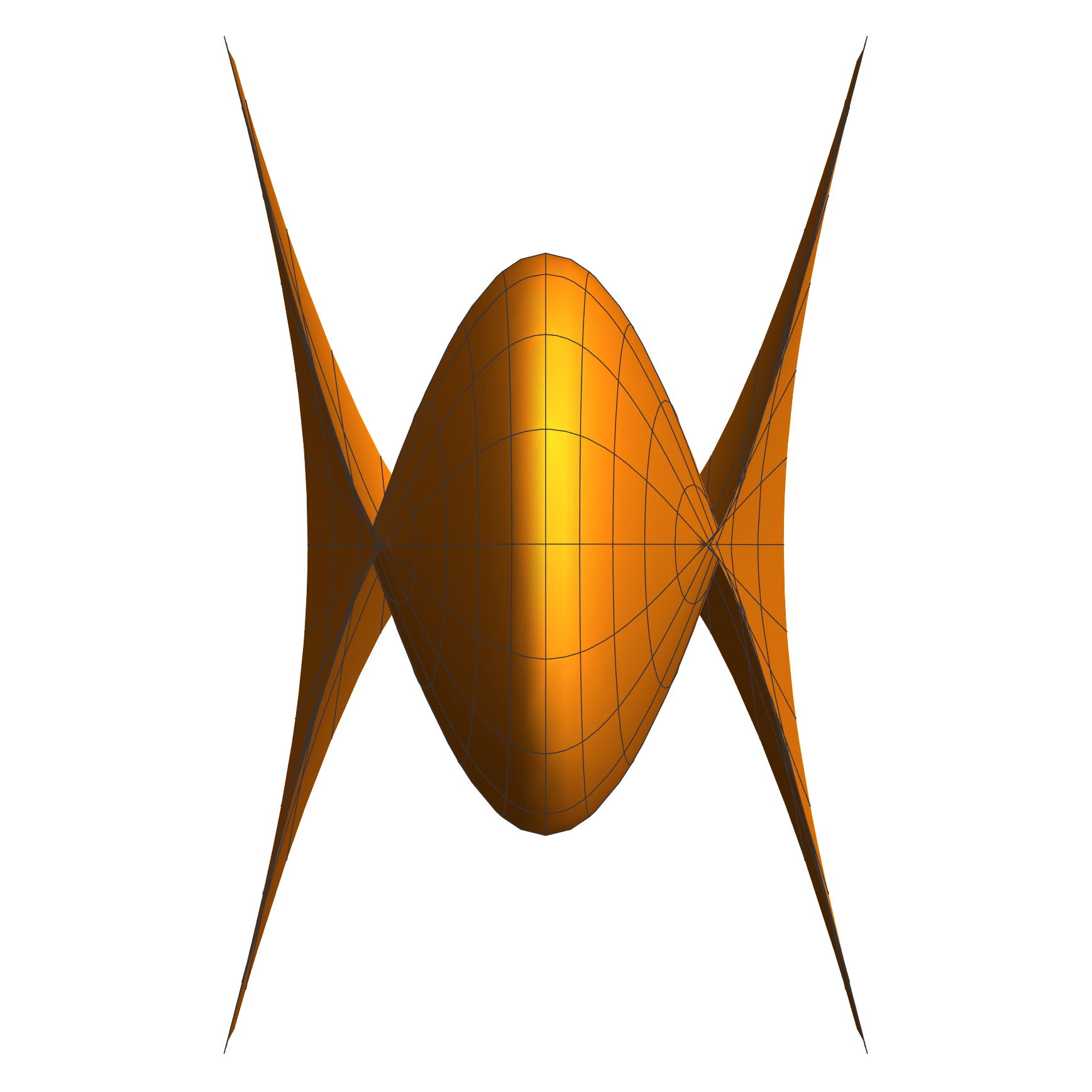
Enneper surface with $K<0$

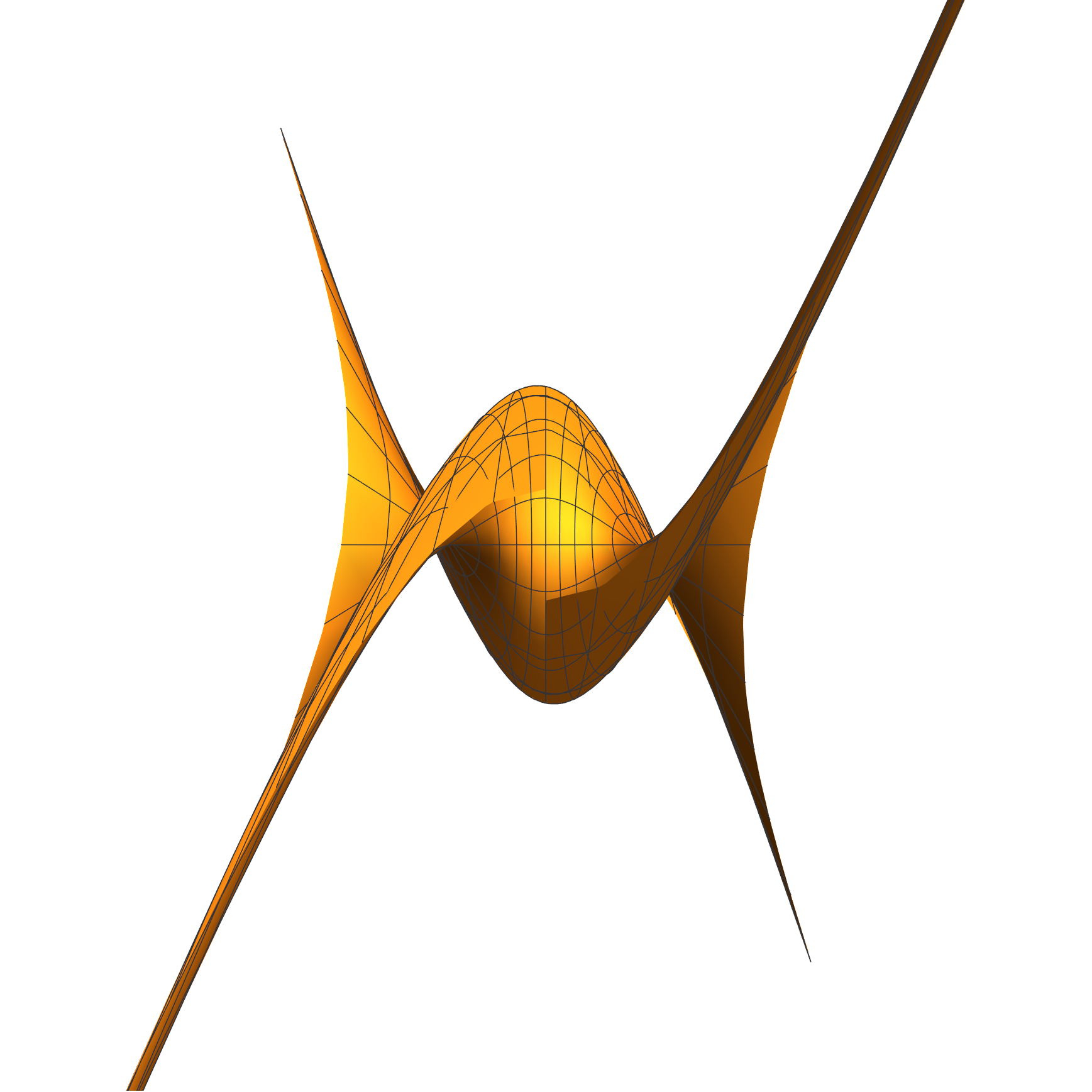
Enneper surface with $K>0$

Figure 1. Enneper surfaces

Conversely, every minimal timelike surface can be obtained at least locally in this way. Note, however, that a minimal timelike surface can be generated via the Weierstrass formula by different pairs of holomorphic functions on the algebra of double numbers.

In his study of minimal timelike surfaces in $\mathbb{R}^{3}_{1}$, G. Ganchev [7] specialized the Weierstrass formula by introducing special isothermal parameters, called canonical. If the surface is parametrized with respect to canonical parameters, then the coefficients of the first and second fundamental forms are

(2.1) $$\begin{array}[]{l}\displaystyle-E=G=\frac{1}{\sqrt{-K}}>0,\qquad F=0,\vspace{1mm}\\ \displaystyle L=-1,\qquad M=0,\qquad N=-1,\end{array}$$

in the case of minimal surfaces of negative Gauss curvature $K$, and

(2.2) $$\begin{array}[]{l}\displaystyle E=-G=\frac{1}{\sqrt{K}}>0,\qquad F=0,\\ \displaystyle L=0,\qquad M=1,\qquad N=0,\end{array}$$

in the case of minimal surfaces of positive Gauss curvature $K$. Note that, because of (2.1) the parametric lines are principal in the case of minimal surfaces with $K<0$. Analogously, because of (2.2) the parametric lines are asymptotic in the case of minimal surfaces with $K>0$. The idea of Ganchev leads to the special Weierstrass curve

(2.3) $$\Phi(z)=\int_{z_{0}}^{z}\,\left(-\frac{1}{2}\,\frac{1+g^{2}(z)}{g^{\prime}(z)},\frac{\mathrm{j}}{2}\,\frac{1-g^{2}(z)}{g^{\prime}(z)},\frac{g(z)}{g^{\prime}(z)}\right)\,dz\ .$$

The real (resp. the ”imaginary”) part of this curve is a minimal timelike surface with canonical parametrization and negative (resp. positive) Gauss curvature. We shall use also the following theorem:

Theorem A [7]. If a timelike surface in $\mathbb{R}^{3}_{1}$ with non-vanishing Gauss curvature is parametrized by canonical parameters $(u,v)$, then the Gauss curvature $K$ satisfies the equation

$$(\ln\sqrt{-K})_{uu}-(\ln\sqrt{-K})_{vv}=2\sqrt{-K},$$

in the case $K<0$, and

$$(\ln\sqrt{K})_{uu}-(\ln\sqrt{K})_{vv}=2\sqrt{K},$$

in the case $K>0$. Conversely, for any solution $K(u,v)$ of any of these equations there exists a unique (up to position in the space) minimal timelike surface of Gauss curvature $K(u,v)$, $(u,v)$ being canonical parameters.

The canonical parameters $(u,v)$ are determined uniquely up to the following transformations [7]:

(2.4) $$\begin{array}[]{l}\vspace{2mm}u=\varepsilon\bar{u}+A\\ \vspace{2mm}v=\varepsilon\bar{v}+B\end{array}\qquad\varepsilon=\pm 1\ ,\ A=const,\ B=const.$$

The idea of canonical parameters is further developed for the class of timelike surfaces in $\mathbb{R}^{n}_{1}$, see [8].

3. Transformation of the isothermal parameters to canonical ones

Suppose the surface $S$ is defined as the real part of the Weierstrass curve

(3.1) $$\Psi(z)=\int_{z_{0}}^{z}\,\left(-\frac{1}{2}\,f(z)(1+g^{2}(z)),\frac{\mathrm{j}}{2}\,f(z)(1-g^{2}(z)),f(z)g(z)\right)\,dz\ .$$

We look for a transformation $z=z(w)$ such that the curve $\Phi(w)=\Psi(z(w))$ has the form

$$\Phi(w)=\int_{w_{0}}^{w}\,\left(-\frac{1}{2}\,\frac{1+\tilde{g}^{2}(w)}{\tilde{g}^{\prime}(w)},\frac{\mathrm{j}}{2}\,\frac{(1-\tilde{g}^{2}(w))}{\tilde{g}^{\prime}(w)},\frac{\tilde{g}(w)}{\tilde{g}^{\prime}(w)}\right)\,dw$$

for some holomorphic function $\tilde{g}(w)$. The real part of this curve will be a canonical representation of the given surface $S$. The equality  $\Psi(z(w))=\Phi(w)$  implies $\Psi^{\prime}(z(w))z^{\prime}(w)=\Phi^{\prime}(w)$. Hence, it is easy to derive

(3.2) $$f(z(w))z^{\prime}(w)=\frac{1}{\tilde{g}^{\prime}(w)}\ ,\qquad\qquad g(z(w))=\tilde{g}(w)\ .$$

The last equality implies

$$\tilde{g}^{\prime}(w)=g^{\prime}(z(w))z^{\prime}(w)$$

and using the first equality of (3.2) we obtain

(3.3) $$(z^{\prime}(w))^{2}=\frac{1}{f(z(w))g^{\prime}(z(w))}\ .$$

Now, we know also the function $\tilde{g}(w)=g(z(w))$ that generates the surface in canonical parameters.

Similar considerations can be done in the case the surface is defined as the ”imaginary” part of the Weierstrass curve determined by (3.1).

So, we can state the following result:

Theorem 3.1.

Let the minimal timelike surface $S$ be defined by the real or ”imaginary” part of (3.1). Any solution to differential equation (3.3) defines a transformation of the isothermal parameters of $S$ to canonical ones. Moreover, the function $\tilde{g}(w)$ that defines $S$ via formula (2.3) is given by $\tilde{g}(w)=g(z(w))$.

As a consequence, we may obtain also relations (2.4) between two different pairs of canonical parameters.

As an application of Theorem 3.1, consider the minimal surfaces $S$ (of negative Gauss curvature) generated by the functions

$$f(z)=a\ ,\qquad g(z)=bz+c$$

via the Weierstrass formula, $a,b,c$ being double numbers, $a\neq 0$, $b\neq 0$, $ab\neq 0$. Equation (3.3) takes the form

$$(z^{\prime}(w))^{2}=\frac{1}{ab}$$

and has the following solution

$$z(w)=\pm\frac{w}{\sqrt{a}\sqrt{b}}+const.$$

According to (2.4) and Theorem 3.1, we may replace $z$ in $g(z)$ with  $\displaystyle{\frac{z}{\sqrt{a}\sqrt{b}}-\frac{c}{b}}$  and we will obtain a parametrization of the surface $S$ in canonical parameters via formula (2.3) and the function

$$\tilde{g}(z)=g\left(\frac{z}{\sqrt{a}\sqrt{b}}-\frac{c}{b}\right)=\frac{\sqrt{b}}{\sqrt{a}}\,z\ .$$

The Gauss curvature is given by the following formula:

$$K=-\frac{16\left|\frac{b}{a}\right|^{2}}{\left(1-\left|\frac{b}{a}\right|(u^{2}-v^{2})\right)^{4}}\ .$$

This result shows that the surface $S_{0}$ of negative Gauss curvature generated via the Weierstrass formula by the functions

$$f(z)=\frac{|a|}{|b|}\ ,\qquad g(z)=z,$$

has the same Gauss curvature in canonical parameters. Hence, due to Theorem A we may identify $S$ with $S_{0}$. On the other hand, the Weierstrass formula implies that $S_{0}$ is homothetic to the standard timelike Enneper surface ($a=b=1$) with $K<0$.

So, as in the case of minimal surfaces in the Euclidean space [3], we have

Corollary 3.2.

The minimal timelike surface generated by the pair of linear functions $f(z)=a,\,g(z)=bz+c$ via the Weierstrass formula coincides with the Enneper surface up to position in the space and homothety.

4. Holomorphic functions generating a minimal timelike surface

As we said before, a minimal timelike surface is generated by different pairs of holomorphic functions via the Weierstrass formula. For example, the Enneper surface of negative (resp. positive) Gauss curvature is the real (resp. ”imaginary”) part of the curve defined via the Weierstrass formula by the pair of functions

(4.1) $$f(z)=1;\qquad g(z)=z,$$

but also by

(4.2) $$f(z)=e^{z};\qquad g(z)=e^{z},$$

and, of course, by many others. So, the following natural question arises: under what conditions do two pairs of holomophic functions give rise to one and the same minimal timelike surface via the Weierstrass representation? It is not difficult to prove the following:

Proposition 4.1.

Suppose the pairs $(\tilde{f}(z),\tilde{g}(z))$ and $(f(w),g(w))$ generate two minimal timelike surfaces via the Weierstrass formula. Then, these surfaces coincide (up to translation) if and only if there exists a function $w=w(z)$, such that

$$\tilde{g}(z)=g(w(z))\qquad{\rm and}\qquad\tilde{f}(z)=f(w(z))w^{\prime}(z)\ .$$

For the two pairs (4.1) and (4.2), that generate the Enneper surface, the function $w(z)=e^{z}$ transfers the first pair into the second one.

Similarly, the following question related to formula (2.3) arises: what is the relation between the functions that generate a minimal timelike surface in canonical parameters? A result in this direction is given by the following theorem.

Theorem 4.2.

Let the holomorphic function $g(z)$ (defined on a domain of $\mathbb{D}$) generate a minimal timelike surface $S$ in canonical parameters, i.e. via formula (2.3). Then, for an arbitrary real number $\varphi$ and an arbitrary double number $\alpha$, by the transformations

(4.3) $$\tilde{g}(z)=\pm e^{\varphi j}\frac{\alpha+g(z)}{1+\bar{\alpha}g(z)};\qquad\qquad\tilde{g}(z)=\pm e^{\varphi j}\frac{1}{f(z)},$$

we obtain the same (up to position in the space) surface in canonical parameters. Conversely, any function that generates (up to position) the surface $S$ in canonical parameters may be obtained in this way.

Proof. Let us consider the first transformation. Denote by $S$ the minimal timelike surface of negative Gauss curvature, generated via formula (2.3) by the function $g(z)$ and let $\Psi(z)$ be the corresponding curve. Analogously, we define $\widetilde{S}$ and $\widetilde{\Psi}(z)$.

We may prove that $S$ and $\widetilde{S}$ coincide (up to position) by a direct computation of their Gauss curvatures using the formula

$$K=-\frac{16|g^{\prime}|^{4}}{(1-|g|^{2})^{4}}$$

and applying Theorem A. Now we give another proof, thus clarifying the relation between $S$, $\widetilde{S}$ and transformation (4.3). We have

$$\Psi^{\prime}(z)=\left(-\frac{1+g^{2}(z)}{2g^{\prime}(z)},\mathrm{j}\frac{1-g^{2}(z)}{2g^{\prime}(z)},\frac{g(z)}{g^{\prime}(z)}\right)\ ,$$

$$\widetilde{\Psi}^{\prime}(z)=\left(-\frac{1+\widetilde{g}^{2}(z)}{2\widetilde{g}^{\prime}(z)},\mathrm{j}\frac{1-\widetilde{g}^{2}(z)}{2\widetilde{g}^{\prime}(z)},\frac{\widetilde{g}(z)}{\widetilde{g}^{\prime}(z)}\right)\ .$$

Let $\alpha=a+\mathrm{j}b$, $a,b\in\mathbb{R}$. Define the SO(1,2)-matrices

$$A=\left(\begin{array}[]{ccc}\cosh\varphi&\sinh\varphi&0\\ \sinh\varphi&\cosh\varphi&0\\ 0&0&1\end{array}\right);\qquad\qquad B=\left(\begin{array}[]{ccc}\frac{1+a^{2}+b^{2}}{1-a^{2}+b^{2}}&\frac{-2ab}{1-a^{2}+b^{2}}&\frac{-2a}{1-a^{2}+b^{2}}\vspace{.1cm}\\ \frac{2ab}{1-a^{2}+b^{2}}&\frac{1-a^{2}-b^{2}}{1-a^{2}+b^{2}}&\frac{-2b}{1-a^{2}+b^{2}}\vspace{.1cm}\\ \frac{-2a}{1-a^{2}+b^{2}}&\frac{2b}{1-a^{2}+b^{2}}&\frac{1+a^{2}-b^{2}}{1-a^{2}+b^{2}}\end{array}\right).$$

A straightforward verification shows that

$$A\,B\,\Psi^{\prime}(z)=\widetilde{\Psi}^{\prime}(z)\ .$$

The last equality implies that up to translation

$$A\,B\,{\bf x}(u,v)=\tilde{\bf x}(u,v)\ .$$

Hence, the considered transformation of type (4.3) of the function $g(z)$ corresponds to a motion of the surface $S$.

Conversely, it is clear that any surface that coincides (up to position) with $S$ may be obtained from $S$ using as above two $SO(1,2)$ matrices and a translation.

∎

As an application of Theorem 4.2, we may prove that any polynomial minimal surfaces $S$ which has polynomial parametrization of degree 3 in isothermal coordinates is (up to position and homothety) an Enneper surface. Namely, we have the following result:

Theorem 4.3.

Let the minimal timelike surface $S$ of negative Gauss curvature has polynomial parametrization of degree 3 in isothermal parameters. Then, up to position in space and homothety, $S$ is (a part of) the Enneper surface of negative curvature.

Proof. Suppose that the surface is defined by

$$S\ :\ \ {\bf x}={\bf x}(u,v).$$

Similarly to the case of surfaces in the Euclidean space (see e.g. section 22.4 in [11]), $S$ is the real part of the Weierstrass curve obtained by substituting the double number variables $\displaystyle{\frac{z}{2}}$ and $\displaystyle{\frac{z}{2\mathrm{j}}}$ formally in the places of the real variables $u,v$:

$$\Psi(z)=2{\bf x}\left(\frac{z}{2},\frac{z}{2\mathrm{j}}\right)-{\bf x}(0,0).$$

Using a translation (if necessary) we may assume that ${\bf x}(0,0)=0$. Since the curve $\Psi(z)$ is a cubic polynomial, then

$$\Psi^{\prime}(z)=(\phi_{1}(z),\phi_{2}(z),\phi_{3}(z))=\left(-\frac{f(z)}{2}(1+g^{2}(z)),\frac{\mathrm{j}}{2}f(z)(1-g^{2}(z)),f(z)g(z)\right)\,dz\$$

for some functions $f(z)$ and $g(z)$ and the functions $\phi_{i}(z)$, $i=1,2,3$ are polynomials of degrees at most 2. Moreover, at least one of them is of degree exactly 2. Hence, the same is true for the following three functions

(4.4) $$f(z)=-\phi_{1}+\mathrm{j}\phi_{2};\qquad f(z)g^{2}(z)=-\phi_{1}-\mathrm{j}\phi_{2};\qquad f(z)g(z)=\phi_{3}\ .$$

So, $f(z)$ is a polynomial of degree at most 2. From the third equality of (4.4) we have $g=\displaystyle{\frac{\phi_{3}}{f}}$. Since $\phi_{3}$ and $f$ are polynomials, we may write $g(z)$ in the form

$$g(z)=\frac{P(z)}{Q(z)}\ ,$$

where the polynomials $P(z)$ and $Q(z)$ have no common zeros. If we assume that $Q(z)$ is a constant, then $g(z)$ is a polynomial and having in mind (4.4), we get $f(z)=const$, $g(z)=cz+d$. If we assume that $Q(z)$ is not a constant, then from the second equality of (4.4), we get

$$f(z)\frac{P^{2}(z)}{Q^{2}(z)}=-\phi_{1}-j\phi_{2},$$

which is a polynomial and hence

$$f(z)=\pm(az+b)^{2}=\pm Q^{2}(z)\ .$$

Up to symmetry of the surface, we assume that

$$f(z)=(az+b)^{2},\qquad Q(z)=az+b\ .$$

Now, $\psi_{3}=f(z)g(z)=(az+b)P(z)$ and since it is of degree at most 2, then $P(z)$ is of degree at most 1, i.e. $P(z)=cz+d$.

Hence, we conclude that, up to homothety of the surface, $f(z)$ and $g(z)$ have the form

$$f(z)=(az+b)^{2};\qquad g(z)=\frac{cz+d}{az+b}\ .$$

On the other hand, the Enneper surface is generated in canonical parameters by the pair of functions $f_{1}(z)=1$, $g_{1}(z)=z$ and due to Theorem 4.2 also by the functions

$$g_{2}(z)=e^{\varphi\mathrm{j}}\frac{\alpha+z}{1+\bar{\alpha}z};\qquad\qquad f_{2}(z)=\frac{1}{g_{2}^{\prime}(z)}=e^{-\varphi\mathrm{j}}\frac{(1+\bar{\alpha}z)^{2}}{|\alpha|^{2}-1}.$$

We can change the parameter $z$ by

$$\frac{(a\alpha e^{\varphi\mathrm{j}}-c)z+\alpha be^{\varphi\mathrm{j}}-d}{(\bar{\alpha}c-ae^{\varphi\mathrm{j}})z+\bar{\alpha}d-be^{\varphi\mathrm{j}}}$$

and then the generating functions take the form:

$$f_{3}(z)=\frac{e^{\varphi\mathrm{j}}(1-|\alpha|^{2})(az+b)^{2}}{\Big{(}(\bar{\alpha}c-ae^{\varphi\mathrm{j}})z+\bar{\alpha}d-be^{\varphi\mathrm{j}}\Big{)}^{2}};\qquad\qquad g_{3}(z)=\frac{cz+d}{az+b}.$$

Of course, in the last expressions the parameters are not canonical. Note that we may choose arbitrary $\varphi$ and $\alpha$, so we put

$$e^{\varphi\mathrm{j}}=\frac{\frac{c^{2}}{(bc-ad)^{2}}}{\left|\frac{c^{2}}{(bc-ad)^{2}}\right|};\qquad\qquad\bar{\alpha}=\frac{ae^{\varphi\mathrm{j}}}{c}\ .$$

Then, $f_{3}(z)$ becomes proportional (with real coefficient) to $f(z)$, thus proving the assertion. Note that $bc-ad$ can not be zero (if we assume that $bc-ad=0$, then the surface is planar which is not our case).

∎

Remark 4.1.

The same proposition holds for minimal timelike surfaces of positive Gauss curvature.

Acknowledgments: The authors are partially supported by the National Science Fund, Ministry of Education and Science of Bulgaria under contract KP-06-N52/3.

References

- [1] R. M. B. Chaves, M. P. Dussan, M. Magid, Björling problem for timelike surfaces in the Lorentz-Minkowski space. Math. Anal. Appl. 377 (2), (2011), 481–494. doi: 10.1016/j.jmaa.2010.10.076.
- [2] A. A. Cintra, I. I. Onnis, Enneper representation of minimal surfaces in the three-dimensional Lorentz-Minkowski space. Annali di Matematica, 197 (1), (2018), 21–39. doi: 10.1007/s10231-017-0666-z.
- [3] C. Cosín, J. Monterde, Bézier Surfaces of Minimal Area. Proc. Int. Workshop of Computer Graphics and Geom. Modelig. Lecture Notes of Computer Science, 72–81, Springer-Verlag, 2002.
- [4] S. Erdem, Harmonic maps of Lorentz surfaces, quadratic differentials and paraholomorphicity. Beiträge Algebra Geom. 38 (1) (1997) 19–32.
- [5] A. Fujioka, J. Inoguchi, Timelike surfaces with harmonic inverse mean curvature, in: Surveys on Geometry and Integrable Systems, in: Adv. Stud. Pure Math., vol. 51, Math. Soc. of Japan, Tokyo, 2008, pp. 113–141.
- [6] G. Ganchev, Canonical Weierstrass representation of minimal surfaces in Euclidean space. ArXiv: 0802.2374.
- [7] G. Ganchev, Canonical Representations of Minimal Time-like Surfaces in Minkowski Space and Explicit Solving of Their Natural PDE. (preprint)
- [8] G. Ganchev, K. Kanchev, Canonical coordinates on minimal time-like surfaces in the -dimensional Minkowski space. Serdica Math. J. 45 (2019), 341–372.
- [9] G. Ganchev, K. Kanchev, Canonical coordinates and natural equations for minimal time-like surfaces in . Kodai Mathematical Journal, 43 (3) 2020, 524–572.
- [10] G. Ganchev, V. Mihova, On the invariant theory of Weingarten surfaces in Euclidean space. J. Phys. A, 43, 40(2010),405210, 27 pp.
- [11] A. Gray, E. Abbena, S. Salamon, Modern Differential Geometry of Curves and Surfaces with Mathematica, Third Edition. Chapman and Hall/CRC, 2006.
- [12] J. Inoguchi, M. Toda, Timelike minimal surfaces via loop groups, Acta Appl. Math. 83 (3) (2004) 313–355.
- [13] O. Kassabov, Transition to canonical principal parameters on minimal surfaces. Comput. Aided Geom. Design. 31 (2014), 441–450.
- [14] J. Konderak, A Weierstrass representation theorem for Lorentz surfaces. Complex Var. Theory Appl., 50 (2005), 319–332. doi: 10.1080/02781070500032895.
- [15] J. H. Lira, M. Melo, F. Mercuri, A Weierstrass representation for minimal surfaces in 3-dimensional manifolds. Results. Math., 60, (2011), 311–323. doi: 10.1007/s00025-011-0169-y.
- [16] M. Magid, Timelike surfaces in Lorentz 3-space with prescribed mean curvature and Gauss map, Hokkaido Math. J. 19 (1991), 447–464. DOI: 10.14492/hokmj/1381413979
- [17] B. A. Shipman, P. D. Shipman, D. Packard, Generalized Weierstrass-Enneper representations of Euclidean, spacelike, and timelike surfaces: a unified Lie-algebraic formulation. J. Geom., 108 (2), (2017), 545–563. doi: 10.1007/s00022-016-0358-7.
- [18] K.T.W. Weierstrass, Untersuchung über die Flächen, deren mittlere Krümmung überall gleich null ist, Monatsberichte der Berliner Akademie, 1866, 612–625.