Numerical Unitarity for Binary Dynamics

Abstract

We present a calculation of the conservative two-body Hamiltonian of a compact binary system including a spinning black hole. We include up-to third order corrections in Newton’s constant $G$, all orders in velocity, and linear and quadratic terms in spin. The results are obtained from the classical limit of two-loop scattering amplitudes involving two massive scalars and two massive spin-1 particles minimally coupled to gravity. We discuss the usage of numerical techniques in our computation. In particular we show how the numerical unitarity method is well suited to obtain results of relevance to the physics program of current and future gravitational wave observatories.

1 Introduction

The first observation of gravitational waves by the LIGO-Virgo collaboration [1] started a new era in the study of the universe. Understanding the systems that produce those feeble spacetime perturbations which we detect is critical to make the most of the experimental programs of current and future (third-generation) gravitational wave observatories. The gravitational wave signals for compact binary systems can be described by three well-distinguished parts. First, the inspiral where the compact objects are very far apart, then the merger where the gravitational fields become strong (for example, when even horizons of coalescent black holes touch), and finally the rigndown where an excited black hole evolves into a stable configuration.

Large amount of templates of these waveform signals are required to find gravitational wave events in the data sets collected by experiments. Though nowadays numerical simulations of full evolution in general relativity are possible, they are rather computationally expensive and so semi-analytic models are required to interpolate among simulations in parameter space. One input that these models take are the conservative potential of the compact binary systems during the inspiral phase. In this presentation we focus on the calculation of those potentials as a post-Minkowskian (PM) expansion, that is as a series expansion in Newton’s coupling $G$. Great efforts have been devoted in recent years to compute higher-order terms in the PM expansion. For example, for spinless systems, third-PM corrections have been computed [2, 3, 4, 5, 6, 7, 8] as well as fourth-PM corrections [9, 10, 11, 12].

The computation of PM corrections to systems involving spinning black holes is of great interest as it is expected that they will play a key role in analyzing a good fraction of detected gravitational waves. In this presentation we focus on the third-PM calculation of the conservative potential for a compact binary system including a spinning black hole [13]. Other recent activity include the calculation of the scattering angle, momentum impulse and spin kick to fourth-PM order [14, 15] (see reference therein for further details). It is expected [16] that with the increased sensitivity of third-generation gravitational wave observatories up-to terms $\mathcal{O}(G^{7})$ will be required to describe signals, and so the development of techniques that can efficiently explore higher order correction is a necessity.

We report on our usage of numerical techniques to compute the two-loop scattering amplitudes necessary for our calculation. In particular we discuss the usage of the unitarity method [17, 18, 19, 20, 21], in a numerical variant [22, 23, 24, 25, 26] which is well suited to deal with generic effective field theories, like for example theories of gravity.

2 Scattering Amplitudes from Numerical Unitarity

We study the scattering process of a massive scalar particle with a massive vector (spin-1) particle minimally coupled to gravity. This is described by the Lagrangian:

$$\mathcal{L}={} \sqrt{-g}\left[-\frac{2R}{\kappa^{2}}\ \ +\frac{1}{2}g^{\mu\nu}\partial_{\mu}\phi\partial_{\nu}\phi-\frac{1}{2}m_{\phi}^{2}\phi^{2}\ \ -\frac{1}{4}g^{\mu\alpha}g^{\nu\beta}F_{\alpha\beta}F_{\mu\nu}+\frac{1}{2}m_{A}^{2}g^{\mu\nu}A_{\mu}A_{\nu}\right]\,,$$ (1)

where $\kappa=\sqrt{32\pi G}$ with $G$ Newton’s constant, $\phi$ is a scalar field, $A^{\mu}$ a vector field, $g_{\mu\nu}$ is the metric, $R$ the Ricci scalar, and $F_{\mu\nu}=\partial_{\mu}A_{\nu}-\partial_{\nu}A_{\mu}$. We study the elastic process

$$A(p_{1},\epsilon_{1})+\phi(p_{2})\to\phi(p_{3})+A(p_{4},\epsilon_{4})\ ,$$

with $p_{1}^{2}=p_{4}^{2}=m_{A}^{2}$, $p_{2}^{2}=p_{3}^{2}=m_{\phi}^{2}$, and where $\epsilon_{1,4}$ are the corresponding polarization vectors of the vector particles. We compute the scattering amplitudes, for given polarization choices, numerically employing the Caravel framework [27]. We do this over momentum configurations with values on a particular number field, that of a finite field with a large cardinality. This allows to employ these numeric evaluations to reconstruct the associated analytic expressions (see e.g. [28, 29]). The implementation of Feynman rules from the Lagrangian above has been made with the help of the package xAct [30, 31].

We employ the unitarity method [17, 18, 19, 20, 21] to compute the needed scattering amplitudes. We start by writing an ansatz for the scattering amplitude:

$$\mathcal{M}=\sum_{\Gamma\in\Delta}\sum_{i\in M_{\Gamma}}c_{\Gamma,i}\ \mathcal{I}_{\Gamma,i}\ ,$$

where the sum is over all the master integrals $\{\mathcal{I}_{\Gamma,i}\}$, here classified by a propagator structure $\Gamma$ and a set of master integral indices $M_{\Gamma}$. In the unitarity method we exploit analytic properties of the scattering amplitudes to extract directly the coefficients $\{c_{\Gamma,i}\}$. Furthermore, in an approach well suited for numerical calculations, we introduce an ansatz of the amplitude’s integrand $\mathcal{M}(\ell_{l})$ as

$$\mathcal{M}(\ell_{l})=\sum_{\Gamma}\sum_{k\in Q_{\Gamma}}c_{\Gamma,k}\frac{m_{\Gamma,k}(\ell_{l})}{\prod_{j\in P_{\Gamma}}\rho_{j}}\ .$$ (2)

The outer sum runs over all propagator structures $\Gamma$ encountered in the amplitude. Given our interest in classical effects, the set of propagator structures is considerably reduced with respect to the full quantum amplitude [2, 3]. In Fig. 1 we show all required structures at the two-loop order. The $\rho_{j}$ are inverse propagators present in $\Gamma$, and the functions $\{m_{\Gamma,k}(\ell_{l})\}$ parametrize all integrand insertions (up to a given power counting in loop momenta). Finally, the coefficients $c_{\Gamma,k}$ contain all the process-specific information and are functions of the external kinematics and the dimensional regularization [32] parameter $\epsilon=(4-D)/2$.

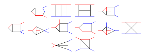
Figure 1: Topologically inequivalent propagator structures contributing to the classical two-body potential. Blue and red lines each represent a massive particle, while black lines denote massless graviton exchanges.

The family of functions $\{m_{\Gamma,k}(\ell_{l})\}$ is labelled by a set of indices $Q_{\Gamma}$. In principle, any complete set (up to a given power counting in the loop momenta) of linearly independent functions can be employed for the ansatz. Typically we use three types of sets. Consider the adaptive loop-momentum parametrization for a given propagator structure $\Gamma$:

$$\ell_{l}=\sum_{j\in B_{l}^{p}}v_{l}^{j}r^{lj}+\sum_{j\in B_{l}^{t}}u_{l}^{j}\alpha^{lj}+\sum_{i\in B^{ct}}\frac{n^{i}}{(n^{i})^{2}}\alpha^{li}+\sum_{k\in B^{\epsilon}}n^{k}\mu_{l}^{k}\ ,$$ (3)

where we have split the $D$-dimensional Minkowski space into four pieces. First, $B_{l}^{p}$ represents the scattering plane spanned by external momenta connected to $\ell_{l}$. Second, $B^{ct}$ is the so-called common-transverse space, the part of the 4-dimensional Minkowski space transverse to all external momenta attached to the propagator structure $\Gamma$. Then $B_{l}^{t}$ is the missing transverse piece to complete the 4-dimensional Minkowski space with the two previous subspaces, and finally we introduce a parametrization of the $\epsilon$-dimensional space with $B^{\epsilon}$. The vectors $v_{l}^{j}$, $u_{l}^{j}$, $n^{i}$, and $n^{k}$, span their corresponding spaces, and the variables left are the corresponding parameters to characterize the loop momenta. In particular the $r^{lj}$ and $\mu_{l}^{k}$ can be associated to inverse propagators of $\Gamma$.

Then when parametrizing a given integrand for a propagator structure $\Gamma$ we can construct the bases:

1. Tensor basis: where we construct from all monomials (up-to corresponding power counting) of the type $(\alpha^{lj})^{\vec{a}}(\alpha^{li})^{\vec{b}}$ with $j\in B_{l}^{t}$ and $i\in B^{ct}$. The vectors $\vec{a}$ and $\vec{b}$ are the non-negative integer exponents of the monomials.

2. Scattering-plane tensor basis: starting from the tensor basis before, we replace all monomials containing variables in $B^{ct}$ by corresponding functions which integrate to zero using one-loop-like surface terms (see e.g. [24]).

3. Master-surface basis: through the usage of unitarity-compatible integration-by-parts (IBP) relations [33] one can further reduce the left-over monomials of the previous basis by surface terms [22] in such way that $Q_{\Gamma}=M_{\Gamma}\cup S_{\Gamma}$ with:

   $$\int\frac{d^{D}\ell_{1}d^{D}\ell_{2}}{(2\pi)^{2D}}\,\frac{m_{\Gamma,i}(\ell_{l})}{\prod_{k\in P_{\Gamma}}\rho_{k}}=\left\{\begin{array}[]{cc}I_{\Gamma,i}&\mbox{for}\quad i\in M_{\Gamma}\ \ \mathrm{{\color[rgb]{0,0,0}\small(master)}}\\ 0&\mbox{for}\quad i\in S_{\Gamma}\ \ \ \mathrm{{\color[rgb]{0,0,0}\small(surface)}}\end{array}\right.$$ (4)

The latter basis is particularly powerful as it trivializes the map between our amplitude integrand ansatz and the integrated form in terms of master integrals. In Caravel we have an automated approach to build the first two types of integrand parametrization and we have collected several master-surface parametrization for amplitudes of interest (see e.g. [34] for more details).

A key factorization property of the integrand of an scattering amplitudes in field theory occurs when we take internal (loop) propagators to on-shell limits. That is, when the inverse propagators go to zero. In this limit equation (2) gives:

$$\sum_{\text{states}}\prod_{i\in T_{\Gamma}}\mathcal{M}_{i}^{\text{tree}}(\ell_{l}^{\Gamma})=\sum_{\begin{subarray}{c}\Gamma^{\prime}\geq\Gamma\\ k\in Q_{\Gamma^{\prime}}\end{subarray}}\frac{{c_{\Gamma^{\prime},k}}\ m_{\Gamma^{\prime},k}(\ell_{l}^{\Gamma})}{\prod_{j\in(P_{\Gamma^{\prime}}/P_{\Gamma})}\rho_{j}(\ell_{l}^{\Gamma})}\ ,$$ (5)

where the sum on the RHS over $\Gamma^{\prime}\geq\Gamma$ means for all propagator structures containing all propagators or more of $\Gamma$. The momenta $\ell_{l}^{\Gamma}$ is such that all inverse propagators in $\Gamma$ vanish. In the LHS of this equation we have the product of all tree-level amplitudes characterized by the vertices of the diagram $\Gamma$. This important relation is called the cut equation [23] and is the one used to compute the coefficients $\{c_{\Gamma,k}\}$ of an scattering amplitude. The process samples multiple values of $\ell_{l}^{\Gamma}$ and through linear algebra techniques, returns all needed coefficients. This is the core of the so-called numerical unitarity method [22, 23, 24, 25, 26].

Whenever we have scattering tensors in our integrand bases, we have employed IBP identities produced with the Fire 6 [35] program. The resulting expression is expanded as a Laurent series in small momentum transfer $q^{2}$ and we also expand the corresponding master integrals accordingly (using [36]). After functional reconstruction, we obtain final analytic expressions for our scattering amplitudes. We refer the reader to the appendices of [13] for the corresponding analytic expressions.

3 Effective Field Theory and Classical Potential

We extract the classical potential through effective field theory (EFT) techniques [37, 38, 39]. For that we employ the non-relativistic EFT described by the Lagrangian:

$$L_{\textrm{EFT}} =\int_{\bm{k}}\hat{\phi}^{\dagger}(-\bm{k})\left(\mathrm{i}\partial_{t}-\sqrt{\bm{k}^{2}+m_{\phi}^{2}}\right)\hat{\phi}(\bm{k})+\int_{\bm{k}}\hat{A}^{\dagger,i}(-\bm{k})\left(\mathrm{i}\partial_{t}-\sqrt{\bm{k}^{2}+m_{A}^{2}}\right)\hat{A}^{i}(\bm{k})$$ (6)

$$-\int_{\bm{k},\bm{k}^{\prime}}\tilde{V}_{ij}(\bm{k},\bm{k}^{\prime})\hat{A}^{\dagger,i}(\bm{k}^{\prime})\hat{A}^{j}(\bm{k})\hat{\phi}^{\dagger}(-\bm{k}^{\prime})\hat{\phi}(-\bm{k})\;,$$

where the integration $\int_{\bm{k}}$ is $\int\frac{d^{3}\bm{k}}{(2\pi)^{3}}$ and the non-local function $\tilde{V}_{ij}$ is the potential which we will obtain according to matching conditions. The potential $\tilde{V}_{ij}$ is decomposed in terms of spin operators, which will produce the different linear (spin-orbit) and quadratic terms in the Lagrangian that we will extract from our calculation.

++

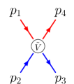
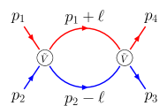
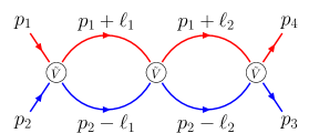
Figure 2: These iterated bubble diagrams give the corresponding amplitude in the effective theory. The blue or red lines represent either the scalar or vector particles.

The EFT amplitude is extracted from iterated bubble diagrams according to [38]. Furthermore the scattering amplitude, as well as the potential $\tilde{V}_{ij}$ is expanded perturbatively in terms of $\kappa$. These expansions are written explicitly in [13]. We perform all calculations in the effective theory in dimensional regularization around $3-2\epsilon$ dimensions. In this way all intermediate steps are properly regularized and the matching procedure systematically removes infrared divergent contributions to both the full theory amplitudes and to the effective theory amplitudes. This is the first time this type of matching procedure has been performed including all dimensional regularization contributions.

After matching the full theory amplitude to the EFT amplitude, order-by-order and up to two loops, we obtained the conservative potential with contributions up to third order in Newton’s constant $G$. For brevity here we only include the spin-orbit term of the potential. Its corresponding coefficient in momentum space we write as $\tilde{c}_{L+1}^{(2)}$, where the $L$ represents the loop order ($L$ is zero for the tree-level result, 1 for one loop, and 2 for two loops). This is decomposed as:

$$\tilde{c}^{(2)}_{L+1} =\tilde{c}^{(2)}_{L+1,\mathrm{red}}+\tilde{c}^{(2)}_{L+1,\mathrm{iter}}+\frac{\tilde{c}^{(1)}_{L+1,\mathrm{red}}}{m_{A}^{2}(\gamma_{1}+1)}\ ,$$ (7)

where $\gamma_{1}=E_{A}/m_{A}$. The coefficients $\tilde{c}^{(1)}_{L+1,\mathrm{red}}$ are the ones appearing in the analogous spinless system. In the end, the full expression for the spin-orbit coefficient up-to $\mathcal{O}(G^{3})$ is:

$$\tilde{c}^{(1)}_{1,\mathrm{red}}(\bm{k}^{2})={} \frac{m_{A}^{2}m_{\phi}^{2}}{E^{2}\xi}\left(1-2\sigma^{2}\right)\,,\qquad\tilde{c}^{(1)}_{2,\mathrm{red}}(\bm{k}^{2})={}\frac{3(m_{\phi}+m_{A})m_{\phi}^{2}m_{A}^{2}}{4E^{2}\xi}(1-5\sigma^{2})\,,$$ (8)

$$\tilde{c}^{(1)}_{3,\mathrm{red}}(\bm{k}^{2})={} \frac{m_{A}^{2}m_{\phi}^{2}}{E^{2}\xi}\left[-\frac{2}{3}m_{A}m_{\phi}\left(\frac{\operatorname{arccosh}(\sigma)}{\sqrt{\sigma^{2}-1}}\left(-12\sigma^{4}+36\sigma^{2}+9\right)+22\sigma^{3}-19\sigma\right)-2(m_{\phi}^{2}+m_{A}^{2})\left(6\sigma^{2}+1\right)\right]$$

$$+\frac{3Em_{A}^{2}m_{\phi}^{2}}{4E^{2}\xi}(m_{A}+m_{\phi})\frac{(1-2\sigma^{2})(1-5\sigma^{2})}{(\sigma^{2}-1)}-\frac{3m_{A}^{4}m_{\phi}^{4}}{E^{2}\xi\bm{k}^{2}}\ ,$$ (9)

$$\tilde{c}^{(2)}_{1,\mathrm{red}}(\bm{k}^{2})={} -\frac{2\sigma m_{\phi}}{E\xi}\ ,\qquad\tilde{c}^{(2)}_{2,\mathrm{red}}(\bm{k}^{2})={}\frac{m_{\phi}(4m_{A}+3m_{\phi})\sigma(5\sigma^{2}-3)}{4E\xi(\sigma^{2}-1)}\ ,$$ (10)

$$\tilde{c}^{(2)}_{3,\mathrm{red}}(\bm{k}^{2})={} \frac{m_{\phi}}{E\xi(\sigma^{2}{-}1)^{2}}\left[\left.{-}2m_{A}^{2}\sigma(3{-}12\sigma^{2}{+}10\sigma^{4}){-}\left(\tfrac{83}{6}{+}27\sigma^{2}{-}52\sigma^{4}{+}\tfrac{44}{3}\sigma^{6}\right)m_{A}m_{\phi}-m_{\phi}^{2}\sigma\left(\tfrac{7}{2}{-}14\sigma^{2}{+}12\sigma^{4}\right)\right.\right.$$

$$\qquad\qquad\qquad\left.{+}\frac{(4m_{A}{+}3m_{\phi})E}{4}\sigma(2\sigma^{2}{-}1)(5\sigma^{2}{-}3){+}4m_{A}m_{\phi}\sigma(\sigma^{2}{-}6)(2\sigma^{2}{+}1)\sqrt{\sigma^{2}{-}1}\operatorname{arccosh}(\sigma)\right]\,,$$ (11)

$$\tilde{c}^{(2)}_{1,\mathrm{iter}}(\bm{k}^{2})={} 0\,,\qquad\tilde{c}^{(2)}_{2,\mathrm{iter}}(\bm{k}^{2})={}E\xi{\tilde{c}}_{1}^{\text{(2)}}\frac{\partial{\tilde{c}}_{1}^{\text{(1)}}}{\partial\bm{k}^{2}}+{\tilde{c}}_{1}^{\text{(1)}}\left(E\xi\frac{\partial{\tilde{c}}_{1}^{\text{(2)}}}{\partial\bm{k}^{2}}+\frac{{\tilde{c}}_{1}^{\text{(2)}}\left(\frac{2E^{2}\xi}{\bm{k}^{2}}+\frac{1}{\xi}-3\right)}{2E}\right)\,,$$ (12)

$$\tilde{c}^{(2)}_{3,\mathrm{iter}}(\bm{k}^{2})={} \left({\tilde{c}}_{1}^{\text{(1)}}\right){}^{2}\left({-}\frac{2}{3}E^{2}\xi^{2}\frac{\partial^{2}{\tilde{c}}_{1}^{\text{(2)}}}{\partial(\bm{k}^{2})^{2}}{+}\left(\xi\left(3{-}\frac{E^{2}\xi}{\bm{k}^{2}}\right){-}1\right)\frac{\partial{\tilde{c}}_{1}^{\text{(2)}}}{\partial\bm{k}^{2}}{+}{\tilde{c}}_{1}^{\text{(2)}}\left(\frac{\frac{1}{2\xi}{-}2}{E^{2}}{+}\frac{3\xi{-}1}{\bm{k}^{2}}\right)\right)$$ (13)

$${+}{\tilde{c}}_{1}^{\text{(1)}}\left({\tilde{c}}_{1}^{\text{(2)}}\left(\left({-}\frac{3E^{2}\xi^{2}}{\bm{k}^{2}}{+}6\xi{-}2\right)\frac{\partial{\tilde{c}}_{1}^{\text{(1)}}}{\partial\bm{k}^{2}}{-}\frac{4}{3}E^{2}\xi^{2}\frac{\partial^{2}{\tilde{c}}_{1}^{\text{(1)}}}{\partial(\bm{k}^{2})^{2}}\right)\right.$$

$$\qquad\qquad\left.{+}\frac{4}{3}E\xi\left(\frac{\partial{\tilde{c}}_{2}^{\text{(2)}}}{\partial\bm{k}^{2}}{-}2E\xi\frac{\partial{\tilde{c}}_{1}^{\text{(1)}}}{\partial\bm{k}^{2}}\frac{\partial{\tilde{c}}_{1}^{\text{(2)}}}{\partial\bm{k}^{2}}\right){+}\frac{E^{2}\xi^{2}\left({\tilde{c}}_{1}^{\text{(2)}}\right){}^{2}}{2\bm{k}^{2}}{+}{\tilde{c}}_{2}^{\text{(2)}}\left(\frac{\frac{2}{3\xi}{-}2}{E}{+}\frac{E\xi}{\bm{k}^{2}}\right)\right){-}\frac{1}{6}E^{2}\xi^{2}\left({\tilde{c}}_{1}^{\text{(2)}}\right){}^{3}$$

$${+}{\tilde{c}}_{1}^{\text{(2)}}\left(\frac{2}{3}E\xi\left(\frac{\partial{\tilde{c}}_{2}^{\text{(1)}}}{\partial\bm{k}^{2}}{-}2E\xi\left(\frac{\partial{\tilde{c}}_{1}^{\text{(1)}}}{\partial\bm{k}^{2}}\right){}^{2}\right){+}\frac{{\tilde{c}}_{2}^{\text{(1)}}\left(\frac{3E^{2}\xi}{\bm{k}^{2}}{+}\frac{1}{\xi}{-}3\right)}{3E}\right){+}\frac{2}{3}E\xi{\tilde{c}}_{2}^{\text{(1)}}\frac{\partial{\tilde{c}}_{1}^{\text{(2)}}}{\partial\bm{k}^{2}}{+}\frac{4}{3}E\xi{\tilde{c}}_{2}^{\text{(2)}}\frac{\partial{\tilde{c}}_{1}^{\text{(1)}}}{\partial\bm{k}^{2}}\,,$$

where $\sigma=\frac{p_{1}\cdot p_{2}}{m_{A}m_{\phi}}$, $E=E_{A}+E_{\phi}$ and $\xi=E_{A}E_{\phi}/E^{2}$. As mentioned above these coefficients are written in momentum space. One can convert to position space if desired by a Fourier transform. We have provided all corresponding expressions as ancillary files to Ref. [13].

We have performed a series of validation tests in our results. In particular our calculation include spinless results which we have systematically compared to the literature [40, 2, 3, 41, 42]. Even more, we have compared to related results in the literature for spinning observables or for post-Newtonian results and found agreement [43, 44, 45, 46, 47, 48, 49].

4 Conclusions

We have presented a calculation including up-to third-order corrections in the Newton’s constant of the conservative potential for a compact binary system including a spinning black hole. The calculation has been performed to all orders in velocity and including up to quadratic terms in spin. We have employed the numerical unitarity method in order to extract analytic expressions for the scattering amplitudes involving massive scalar and massive vector particles minimally coupled to gravity. This framework is flexible enough to carry further calculations of interest to the future of gravitational wave astronomy. In particular it is possible to explore higher spin terms, finite-size effects, and even higher loop corrections.

References

- [1] B. P. Abbott et al. [LIGO Scientific and Virgo], “Observation of Gravitational Waves from a Binary Black Hole Merger,” Phys. Rev. Lett. 116, no.6, 061102 (2016) doi:10.1103/PhysRevLett.116.061102 [arXiv:1602.03837 [gr-qc]].
- [2] Z. Bern, C. Cheung, R. Roiban, C. H. Shen, M. P. Solon and M. Zeng, “Scattering Amplitudes and the Conservative Hamiltonian for Binary Systems at Third Post-Minkowskian Order,” Phys. Rev. Lett. 122, no.20, 201603 (2019) doi:10.1103/PhysRevLett.122.201603 [arXiv:1901.04424 [hep-th]].
- [3] Z. Bern, C. Cheung, R. Roiban, C. H. Shen, M. P. Solon and M. Zeng, “Black Hole Binary Dynamics from the Double Copy and Effective Theory,” JHEP 10, 206 (2019) doi:10.1007/JHEP10(2019)206 [arXiv:1908.01493 [hep-th]].
- [4] G. Kälin, Z. Liu and R. A. Porto, “Conservative Dynamics of Binary Systems to Third Post-Minkowskian Order from the Effective Field Theory Approach,” Phys. Rev. Lett. 125, no.26, 261103 (2020) doi:10.1103/PhysRevLett.125.261103 [arXiv:2007.04977 [hep-th]].
- [5] P. Di Vecchia, C. Heissenberg, R. Russo and G. Veneziano, “The eikonal approach to gravitational scattering and radiation at (G3),” JHEP 07, 169 (2021) doi:10.1007/JHEP07(2021)169 [arXiv:2104.03256 [hep-th]].
- [6] E. Herrmann, J. Parra-Martinez, M. S. Ruf and M. Zeng, “Radiative classical gravitational observables at (G3) from scattering amplitudes,” JHEP 10, 148 (2021) doi:10.1007/JHEP10(2021)148 [arXiv:2104.03957 [hep-th]].
- [7] N. E. J. Bjerrum-Bohr, P. H. Damgaard, L. Planté and P. Vanhove, “The amplitude for classical gravitational scattering at third Post-Minkowskian order,” JHEP 08, 172 (2021) doi:10.1007/JHEP08(2021)172 [arXiv:2105.05218 [hep-th]].
- [8] A. Brandhuber, G. Chen, G. Travaglini and C. Wen, “Classical gravitational scattering from a gauge-invariant double copy,” JHEP 10, 118 (2021) doi:10.1007/JHEP10(2021)118 [arXiv:2108.04216 [hep-th]].
- [9] Z. Bern, J. Parra-Martinez, R. Roiban, M. S. Ruf, C. H. Shen, M. P. Solon and M. Zeng, “Scattering Amplitudes and Conservative Binary Dynamics at ,” Phys. Rev. Lett. 126, no.17, 171601 (2021) doi:10.1103/PhysRevLett.126.171601 [arXiv:2101.07254 [hep-th]].
- [10] Z. Bern, J. Parra-Martinez, R. Roiban, M. S. Ruf, C. H. Shen, M. P. Solon and M. Zeng, “Scattering Amplitudes, the Tail Effect, and Conservative Binary Dynamics at O(G4),” Phys. Rev. Lett. 128, no.16, 161103 (2022) doi:10.1103/PhysRevLett.128.161103 [arXiv:2112.10750 [hep-th]].
- [11] C. Dlapa, G. Kälin, Z. Liu and R. A. Porto, “Dynamics of binary systems to fourth Post-Minkowskian order from the effective field theory approach,” Phys. Lett. B 831, 137203 (2022) doi:10.1016/j.physletb.2022.137203 [arXiv:2106.08276 [hep-th]].
- [12] C. Dlapa, G. Kälin, Z. Liu and R. A. Porto, “Conservative Dynamics of Binary Systems at Fourth Post-Minkowskian Order in the Large-Eccentricity Expansion,” Phys. Rev. Lett. 128, no.16, 161104 (2022) doi:10.1103/PhysRevLett.128.161104 [arXiv:2112.11296 [hep-th]].
- [13] F. Febres Cordero, M. Kraus, G. Lin, M. S. Ruf and M. Zeng, “Conservative Binary Dynamics with a Spinning Black Hole at O(G3) from Scattering Amplitudes,” Phys. Rev. Lett. 130, no.2, 021601 (2023) doi:10.1103/PhysRevLett.130.021601 [arXiv:2205.07357 [hep-th]].
- [14] G. U. Jakobsen, G. Mogull, J. Plefka, B. Sauer and Y. Xu, “Conservative Scattering of Spinning Black Holes at Fourth Post-Minkowskian Order,” Phys. Rev. Lett. 131, no.15, 151401 (2023) doi:10.1103/PhysRevLett.131.151401 [arXiv:2306.01714 [hep-th]].
- [15] G. U. Jakobsen, G. Mogull, J. Plefka and B. Sauer, “Dissipative scattering of spinning black holes at fourth post-Minkowskian order,” [arXiv:2308.11514 [hep-th]].
- [16] A. Buonanno, M. Khalil, D. O’Connell, R. Roiban, M. P. Solon and M. Zeng, “Snowmass White Paper: Gravitational Waves and Scattering Amplitudes,” [arXiv:2204.05194 [hep-th]].
- [17] Z. Bern, L. J. Dixon, D. C. Dunbar and D. A. Kosower, “One loop n point gauge theory amplitudes, unitarity and collinear limits,” Nucl. Phys. B 425, 217-260 (1994) doi:10.1016/0550-3213(94)90179-1 [arXiv:hep-ph/9403226 [hep-ph]].
- [18] Z. Bern, L. J. Dixon, D. C. Dunbar and D. A. Kosower, “Fusing gauge theory tree amplitudes into loop amplitudes,” Nucl. Phys. B 435, 59-101 (1995) doi:10.1016/0550-3213(94)00488-Z [arXiv:hep-ph/9409265 [hep-ph]].
- [19] Z. Bern and A. G. Morgan, “Massive loop amplitudes from unitarity,” Nucl. Phys. B 467, 479-509 (1996) doi:10.1016/0550-3213(96)00078-8 [arXiv:hep-ph/9511336 [hep-ph]].
- [20] Z. Bern, L. J. Dixon and D. A. Kosower, “One loop amplitudes for e+ e- to four partons,” Nucl. Phys. B 513, 3-86 (1998) doi:10.1016/S0550-3213(97)00703-7 [arXiv:hep-ph/9708239 [hep-ph]].
- [21] R. Britto, F. Cachazo and B. Feng, “Generalized unitarity and one-loop amplitudes in N=4 super-Yang-Mills,” Nucl. Phys. B 725, 275-305 (2005) doi:10.1016/j.nuclphysb.2005.07.014 [arXiv:hep-th/0412103 [hep-th]].
- [22] H. Ita, “Two-loop Integrand Decomposition into Master Integrals and Surface Terms,” Phys. Rev. D 94, no.11, 116015 (2016) doi:10.1103/PhysRevD.94.116015 [arXiv:1510.05626 [hep-th]].
- [23] S. Abreu, F. Febres Cordero, H. Ita, M. Jaquier and B. Page, “Subleading Poles in the Numerical Unitarity Method at Two Loops,” Phys. Rev. D 95, no.9, 096011 (2017) doi:10.1103/PhysRevD.95.096011 [arXiv:1703.05255 [hep-ph]].
- [24] S. Abreu, F. Febres Cordero, H. Ita, M. Jaquier, B. Page and M. Zeng, “Two-Loop Four-Gluon Amplitudes from Numerical Unitarity,” Phys. Rev. Lett. 119, no.14, 142001 (2017) doi:10.1103/PhysRevLett.119.142001 [arXiv:1703.05273 [hep-ph]].
- [25] S. Abreu, F. Febres Cordero, H. Ita, B. Page and M. Zeng, “Planar Two-Loop Five-Gluon Amplitudes from Numerical Unitarity,” Phys. Rev. D 97, no.11, 116014 (2018) doi:10.1103/PhysRevD.97.116014 [arXiv:1712.03946 [hep-ph]].
- [26] S. Abreu, F. Febres Cordero, H. Ita, B. Page and V. Sotnikov, “Planar Two-Loop Five-Parton Amplitudes from Numerical Unitarity,” JHEP 11, 116 (2018) doi:10.1007/JHEP11(2018)116 [arXiv:1809.09067 [hep-ph]].
- [27] S. Abreu, J. Dormans, F. Febres Cordero, H. Ita, M. Kraus, B. Page, E. Pascual, M. S. Ruf and V. Sotnikov, “Caravel: A C++ framework for the computation of multi-loop amplitudes with numerical unitarity,” Comput. Phys. Commun. 267, 108069 (2021) doi:10.1016/j.cpc.2021.108069 [arXiv:2009.11957 [hep-ph]].
- [28] A. von Manteuffel and R. M. Schabinger, “A novel approach to integration by parts reduction,” Phys. Lett. B 744, 101-104 (2015) doi:10.1016/j.physletb.2015.03.029 [arXiv:1406.4513 [hep-ph]].
- [29] T. Peraro, “Scattering amplitudes over finite fields and multivariate functional reconstruction,” JHEP 12, 030 (2016) doi:10.1007/JHEP12(2016)030 [arXiv:1608.01902 [hep-ph]].
- [30] D. Brizuela, J. M. Martin-Garcia and G. A. Mena Marugan, “xPert: Computer algebra for metric perturbation theory,” Gen. Rel. Grav. 41, 2415-2431 (2009) doi:10.1007/s10714-009-0773-2 [arXiv:0807.0824 [gr-qc]].
- [31] T. Nutma, “xTras : A field-theory inspired xAct package for mathematica,” Comput. Phys. Commun. 185, 1719-1738 (2014) doi:10.1016/j.cpc.2014.02.006 [arXiv:1308.3493 [cs.SC]].
- [32] G. ’t Hooft and M. J. G. Veltman, “Regularization and Renormalization of Gauge Fields,” Nucl. Phys. B 44, 189-213 (1972) doi:10.1016/0550-3213(72)90279-9
- [33] J. Gluza, K. Kajda and D. A. Kosower, “Towards a Basis for Planar Two-Loop Integrals,” Phys. Rev. D 83, 045012 (2011) doi:10.1103/PhysRevD.83.045012 [arXiv:1009.0472 [hep-th]].
- [34] S. Abreu, F. Febres Cordero, H. Ita, M. Jaquier, B. Page, M. S. Ruf and V. Sotnikov, “Two-Loop Four-Graviton Scattering Amplitudes,” Phys. Rev. Lett. 124, no.21, 211601 (2020) doi:10.1103/PhysRevLett.124.211601 [arXiv:2002.12374 [hep-th]].
- [35] A. V. Smirnov and F. S. Chuharev, “FIRE6: Feynman Integral REduction with Modular Arithmetic,” Comput. Phys. Commun. 247 , 106877 (2020) doi:10.1016/j.cpc.2019.106877 [arXiv:1901.07808 [hep-ph]].
- [36] J. Parra-Martinez, M. S. Ruf and M. Zeng, “Extremal black hole scattering at : graviton dominance, eikonal exponentiation, and differential equations,” JHEP 11, 023 (2020) doi:10.1007/JHEP11(2020)023 [arXiv:2005.04236 [hep-th]].
- [37] D. Neill and I. Z. Rothstein, “Classical Space-Times from the S Matrix,” Nucl. Phys. B 877, 177-189 (2013) doi:10.1016/j.nuclphysb.2013.09.007 [arXiv:1304.7263 [hep-th]].
- [38] C. Cheung, I. Z. Rothstein and M. P. Solon, “From Scattering Amplitudes to Classical Potentials in the Post-Minkowskian Expansion,” Phys. Rev. Lett. 121, no.25, 251101 (2018) doi:10.1103/PhysRevLett.121.251101 [arXiv:1808.02489 [hep-th]].
- [39] Z. Bern, A. Luna, R. Roiban, C. H. Shen and M. Zeng, “Spinning black hole binary dynamics, scattering amplitudes, and effective field theory,” Phys. Rev. D 104, no.6, 065014 (2021) doi:10.1103/PhysRevD.104.065014 [arXiv:2005.03071 [hep-th]].
- [40] B. R. Holstein and A. Ross, “Spin Effects in Long Range Gravitational Scattering,” [arXiv:0802.0716 [hep-ph]].
- [41] A. Cristofoli, P. H. Damgaard, P. Di Vecchia and C. Heissenberg, “Second-order Post-Minkowskian scattering in arbitrary dimensions,” JHEP 07, 122 (2020) doi:10.1007/JHEP07(2020)122 [arXiv:2003.10274 [hep-th]].
- [42] D. Kosmopoulos and A. Luna, “Quadratic-in-spin Hamiltonian at (G2) from scattering amplitudes,” JHEP 07, 037 (2021) doi:10.1007/JHEP07(2021)037 [arXiv:2102.10137 [hep-th]].
- [43] M. Levi and J. Steinhoff, “Next-to-next-to-leading order gravitational spin-squared potential via the effective field theory for spinning objects in the post-Newtonian scheme,” JCAP 01, 008 (2016) doi:10.1088/1475-7516/2016/01/008 [arXiv:1506.05794 [gr-qc]].
- [44] M. Levi and J. Steinhoff, “Next-to-next-to-leading order gravitational spin-orbit coupling via the effective field theory for spinning objects in the post-Newtonian scheme,” JCAP 01, 011 (2016) doi:10.1088/1475-7516/2016/01/011 [arXiv:1506.05056 [gr-qc]].
- [45] M. Levi and J. Steinhoff, “EFTofPNG: A package for high precision computation with the Effective Field Theory of Post-Newtonian Gravity,” Class. Quant. Grav. 34, no.24, 244001 (2017) doi:10.1088/1361-6382/aa941e [arXiv:1705.06309 [gr-qc]].
- [46] J. Vines, “Scattering of two spinning black holes in post-Minkowskian gravity, to all orders in spin, and effective-one-body mappings,” Class. Quant. Grav. 35, no.8, 084002 (2018) doi:10.1088/1361-6382/aaa3a8 [arXiv:1709.06016 [gr-qc]].
- [47] J. Vines, J. Steinhoff and A. Buonanno, “Spinning-black-hole scattering and the test-black-hole limit at second post-Minkowskian order,” Phys. Rev. D 99, no.6, 064054 (2019) doi:10.1103/PhysRevD.99.064054 [arXiv:1812.00956 [gr-qc]].
- [48] Z. Liu, R. A. Porto and Z. Yang, “Spin Effects in the Effective Field Theory Approach to Post-Minkowskian Conservative Dynamics,” JHEP 06, 012 (2021) doi:10.1007/JHEP06(2021)012 [arXiv:2102.10059 [hep-th]].
- [49] G. U. Jakobsen and G. Mogull, “Conservative and Radiative Dynamics of Spinning Bodies at Third Post-Minkowskian Order Using Worldline Quantum Field Theory,” Phys. Rev. Lett. 128, no.14, 141102 (2022) doi:10.1103/PhysRevLett.128.141102 [arXiv:2201.07778 [hep-th]].