Generalized Schröder paths arising from a combinatorial interpretation of generalized Laurent bi-orthogonal polynomials

Abstract

Lattice paths called $\ell$-Schröder paths are introduced. They are paths on the upper half-plane consisting of $\ell+2$ types of steps: $(i,\ell-i)$ for $i=0,\ldots,\ell$, and $(1,-1)$. Those paths generalize Schröder paths and some variants, such as $m$-Schröder paths by Yang and Jiang and Motzkin-Schröder paths by Kim and Stanton. We show that $\ell$-Schröder paths arise naturally from a combinatorial interpretation of the moments of generalized Laurent bi-orthogonal polynomials introduced by Wang, Chang, and Yue. We also show that some generating functions of non-intersecting $\ell$-Schröder paths can be factorized in closed forms.

1 Introduction

A Schröder path is a path in the $x$-$y$ plane with three types of elementary steps $(1,0),(0,1)$, and $(1,-1)$, never going below the $x$-axis. Schröder paths are among the well-studied lattice paths in combinatorics, having attracted attention due to their connection with exactly solvable models [8, 16, 1]. A typical example of such a model is the domino tilings of the Aztec diamonds introduced by Elkies et al. [6], which exhibits a one-to-one correspondence with non-intersecting tuples of Schröder paths [10]. Schröder paths have a notable property that certain generating functions of non-intersecting tuplets are expressed in a closed form [12, 7], which is one of the critical ingredients to enumerate solvable models.

In this paper, we propose a generalization of Schröder paths that preserves this notable property of generating functions.

Definition 1.1.

For a positive integer $\ell$, an $\ell$-Schröder path is a lattice path in the $x$-$y$ plane with steps $\mathsf{a}_{i}\triangleq(i,\ell-i)$ for $i=0\ldots,\ell$ and $\mathsf{a}_{\ell+1}\triangleq(1,-1)$, never going below the $x$-axis.

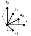
Figure  1: Left: an example of $3$-Schröder path. Right: the five types of steps in $3$-Schröder path.

See Figure 1 for an example of $\ell$-Schröder paths when $\ell=3$.

In the literature, there are several ways to extend Schröder paths. One way is to use steps $(0,m)$ and $(1,m-1)$ instead of $(0,1)$ and $(1,0)$. Such a generalization is called $m$-Schröder paths in [19]. Another way is to add a new step $(1,1)$ to Schröder paths. Such paths are called Motzkin-Schröder paths and were introduced by Kim and Stanton [13] in connection with orthogonal functions. In [13], they found that certain generating functions of non-intersecting tuplet of Motzkin-Schröder paths admit a closed-form factorization. The $\ell$-Schröder paths in this paper essentially contain both $m$-Schröder and Motzkin-Schröder paths as special cases.

The aim of this paper is twofold: (i) to describe that $\ell$-Schröder paths arise naturally from a combinatorial interpretation of orthogonal functions; (ii) to show that certain generating functions of non-intersecting tuplets of $\ell$-Schröder paths are written in closed forms. See Figure 8 in Section 4 for an example of a non-intersecting tuplet that we will consider.

The combinatorial theory of orthogonal polynomials (OPs) was established by Viennot [17] using weighted paths. A similar approach was developed by Kamioka [11, 12] for Laurent bi-orthogonal polynomials (LBPs), the analogue of OPs introduced in the field of two-point Padé approximation and discrete integrable systems [20]. In a series of his studies, Kamioka interpreted LBPs using weighted Schröder paths.

LBPs are, as in OPs, characterized by so-called the fundamental three-term recurrence relation [20]

$$P_{n+1}(x)=(x-d_{n})P_{n}(x)-b_{n}xP_{n-1}(x),$$ (1)

where $d_{n}$ and $b_{n}$ are non-zero. Generalizations of LBPs are obtained by increasing the number of terms in the recurrence as

$$P_{n}(x)=-\sum_{i=1}^{\ell-1}a_{i,n-\ell}P_{n-i}(x)+(x^{\ell}-a_{\ell,n-\ell})P_{n-\ell}(x)-a_{\ell+1,n-\ell}x^{\ell}P_{n-\ell-1}(x),\quad n\geq\ell,$$ (2)

where $a_{\ell,i}$ and $a_{\ell+1,i}$ are non-vanishing, and the other $a_{i,j}$ are some constants. Such generalized LBPs are studied by several authors [18, 14, 3]. We refer to these generalized LBPs as $\ell$-LBPs since the letter $\ell$ is used as a fixed parameter in [18]. We show that $\ell$-Schröeder paths emerge from a combinatorial interpretation of $\ell$-LBPs.

To show the second aim of this paper, we employ the technique developed by Eu and Fu [7]. They enumerate non-intersecting tuplets of Schröder paths in closed form by combining two kinds of paths, i.e., Schröder and small Schröder paths. We define new paths called small $\ell$-Schröder paths and generalize their technique.

This paper is organized as follows: In Section 2, we recall the definition and fundamentals of $\ell$-LBPs and present a Favard-type theorem essential for a combinatorial interpretation. In Section 3, we interpret the moments of $\ell$-LBPs using $\ell$-Schröder paths (Theorem 3.2). This theorem parallels the Kamioka development [11] for conventional LBPs. In section 4, we examine the enumerative aspects of $\ell$-Schröder paths. We explore the relationship between $\ell$-Schröder paths and small $\ell$-Schröder paths. Using the methods of Eu and Fu [7], we express generating functions of non-intersecting $\ell$-Schröder paths in a closed form (Theorem 4.10). As an application of the results in this chapter, we discuss specialized generating functions of $\ell$-Schröder paths, namely the $\ell$-Narayana polynomials.

2 $\ell$-LBPs and Favard-type theorem

In this section, we briefly review the fundamentals of $\ell$-LBPs, including their definitions, recurrence relations, Favard-type theorem, and determinant expressions.

Let $\mathbb{K}$ be a field, and $\mathbb{N}_{0}$ be the set of non-negative integers. Let $\mathcal{L}\colon\mathbb{K}[x,x^{-1}]\to\mathbb{K}$ be a linear functional on the space of Laurent polynomials over $\mathbb{K}$. A sequence of monic polynomials $(P_{n}(x))_{n=0}^{\infty}$ with each $P_{n}(x)$ having exact degree $n$ is called an $\ell$-Laurent bi-orthogonal polynomials ($\ell$-LBPs) with respect to $\mathcal{L}$ if it satisfies the orthogonality

$$\mathcal{L}\left[P_{n}(x)x^{-k\ell}\right]=h_{n}\delta_{nk},\qquad n,k\in\mathbb{N}_{0},\ 0\leq k\leq n$$ (3)

for some non-vanishing constant $h_{n}\neq 0$. The symbol $\delta_{n,k}$ denotes the Kronecker delta. In the case $\ell=1$, the conventional LBPs are recovered.

Each polynomial $P_{n}(x)$ in $\ell$-LBPs satisfies the $(\ell+2)$-term recurrence relation (2) for $n\geq\ell$ (cf. [18]). Conversely, the following theorem states that any sequence of polynomials defined by the recurrence (2) with suitable initial condition is a $\ell$-LBPs.

Theorem 2.1 (Favard-type theorem for $\ell$-LBPs).

Let $a_{i,j}\in\mathbb{K}$ be constants such that $a_{\ell,i}\neq 0$ and $a_{\ell+1,i}\neq 0$ for all $i\in\mathbb{N}_{0}$. Let $p_{n}(x)\in\mathbb{K}[x]$ be monic polynomials of degree $n$ for $n=0,\ldots,\ell-1$. The sequence of polynomials $(P_{n}(x))_{n=0}^{\infty}$ defined by the recurrence (2) with initial conditions $P_{-1}(x)\triangleq 0$ and $P_{n}(x)\triangleq p_{n}(x)$ for $n=0,\ldots,\ell-1$, is an $\ell$-LBPs with respect to some linear functional $\mathcal{L}$. Furthermore, if we impose the condition $\mathcal{L}[1]=1$, such a linear functional $\mathcal{L}$ is uniquely determined.

Theorem 2.1 is fundamental in the theory of $\ell$-LBPs. However, the author cannot find the reference that explicitly provides its proof, so we prove it here. We need a lemma to prove Theorem 2.1.

Lemma 2.2.

Let $(P_{n}(x))_{n=0}^{\infty}$ be as in Theorem 2.1. For any non-negative integer $k\in\mathbb{N}_{0}$, we have

$$\det\left([x^{j}]P_{k+i}(x)\right)_{i,j=0}^{\ell-1}=(-1)^{k\ell}\prod_{i=0}^{k-1}a_{\ell,i},$$ (4)

where $[x^{j}]P_{k+i}(x)$ denotes the coefficients of $x^{j}$ in the polynomial $P_{k+i}(x)$.

Proof.

Let $T_{k}\triangleq\det([x^{j}]P_{k+i}(x))_{i,j=0}^{\ell-1}$ be the left-hand side of (4). We derive a recurrence for $T_{k}$. It is easy to check that $T_{0}=1$ by using the monicity of $p_{k}(x)$ for $k=0,\ldots,\ell-1$.

Let us think about $T_{k}$ for $k\geq 1$. By multiplying the first column by $a_{\ell,k}$, we get

$$a_{\ell,k}T_{k}=\det\left[\begin{array}[]{cccc}\left[x^{0}\right]a_{\ell,k}P_{k}(x)&\left[x^{0}\right]P_{k+1}(x)&\cdots&\left[x^{0}\right]P_{k+\ell-1}(x)\\ \vdots&&&\vdots\\ \left[x^{\ell-1}\right]a_{\ell,k}P_{k}(x)&\left[x^{\ell-1}\right]P_{k+1}(x)&\cdots&\left[x^{\ell-1}\right]P_{k+\ell-1}(x)\end{array}\right].$$ (8)

Multiplying the $j$-th column by $a_{\ell-j,k}$ and adding it to the first ($0$-th) column for $j=1,\ldots,\ell-1$ we have

$$a_{\ell,k}T_{k}=\det\left[\begin{array}[]{cccc}\left[x^{0}\right]F_{k}&\left[x^{0}\right]P_{k+1}(x)&\cdots&\left[x^{0}\right]P_{k+\ell-1}(x)\\ \vdots&&&\vdots\\ \left[x^{\ell-1}\right]F_{k}&\left[x^{\ell-1}\right]P_{k+1}(x)&\cdots&\left[x^{\ell-1}\right]P_{k+\ell-1}(x)\end{array}\right],$$ (12)

where we write $F_{k}\triangleq\sum_{i=1}^{\ell}a_{i,k}P_{k+\ell-i}$. From the recurrence (2), we have $[x^{i}]F_{k}=-[x^{i}]P_{k+\ell}$ for $k\geq 0$ and $i=0,\ldots,\ell-1$. Substituting this into (12), we get the recurrence $T_{k+1}=(-1)^{\ell}a_{\ell,k}T_{k}$ for $k\geq 0$. ∎

Proof of Theorem 2.1.

We define a linear functional $\mathcal{L}$ by defining its moments $\mu_{n}=\mathcal{L}[x^{n}]\ (n\in\mathbb{Z})$ inductively on $n$. Let us define the positive-side moments $\mu_{n}\ (n\geq 0)$ by $\mathcal{L}[1]=1$ and equations

$$\mathcal{L}[P_{n}(x)]=0,\qquad n=1,2,3,\ldots.$$ (13)

Also, define the negative-side moments $\mu_{n}\ (n<0)$ by solving the system of equations

$$\mathcal{L}[P_{n+i}(x)x^{-n\ell}]=0,\qquad i=1,\ldots,\ell$$ (14)

for $n=1,2,\ldots$, as Lemma 2.2 shows the system (14) has a unique solution. Note that the moments $\mu_{-\ell n+i}\ (i=0,1,\ldots,\ell-1)$ are determined from equations (14). This process determines the moments $\mu_{n}\ (n\in\mathbb{Z})$ uniquely.

Next, we show that the linear functional $\mathcal{L}$ defined by the moments $\mu_{n}\ (n\in\mathbb{Z})$ as above satisfies the orthogonality

$$\mathcal{L}[P_{n}(x)x^{-k\ell}] =0,\qquad k,n\in\mathbb{N}_{0},k<n,\ {\rm and}$$ (15)

$$\mathcal{L}[P_{n}(x)x^{-n\ell}] \neq 0,\qquad n\in\mathbb{N}_{0}.$$ (16)

The equations (15) hold for $k=0$ and $k=n-\ell,\ldots,n-1$ by the definition of the moments. In other words, the equation (15) is already shown when $n\leq\ell+1$. Therefore, we show the remaining cases $n\geq\ell+2$ by induction on $n$. Assume that (15) holds for all $n$ less than $N$, where $N\geq\ell+2$. Using the recurrence (2), one can write $\mathcal{L}[P_{N}(x)x^{-k\ell}]$ as a linear combination of $\mathcal{L}[P_{N-i}(x)x^{-k\ell}]\ (i=1,\ldots,\ell-1),\ \mathcal{L}[P_{N-\ell}(x)x^{-(k-1)\ell}],\ \mathcal{L}[P_{N-\ell}(x)x^{-k\ell}]$, and $\mathcal{L}[P_{N-\ell-1}(x)x^{-(k-1)\ell}]$, all of which are zero by the inductive hypothesis. Thus (15) holds when $n=N$.

The equation (16) is shown by a recurrence

$$\mathcal{L}[P_{n}(x)x^{-n\ell}]=-\frac{a_{\ell+1,n}}{a_{\ell,n}}\mathcal{L}[P_{n-1}(x)x^{-(n-1)\ell}],\qquad n\geq 1,$$ (17)

which is derived from multiplying both sides of (2) by $x^{-(n-\ell)\ell}$ and acting $\mathcal{L}$. ∎

Additionally, we would like to discuss the relationship between the moments of $\ell$-LBPs defined by the recurrence (2) with different initial conditions. We define two $\ell$-LBPs as equivalent if they satisfy the recurrence (2) with identical coefficients $a_{i,j}$. The set of all $\ell$-LBPs is divided into equivalence classes based on this equivalence relation. Within each equivalence class, there exists a unique $\ell$-LBPs $(P_{n}(x))_{n=0}^{\infty}$ whose first $\ell$ polynomials are monomials, i.e., $P_{i}(x)=x^{i}$ for $i=0,\ldots,\ell-1$. We refer to such $\ell$-LBPs as primitive. The following theorem states that the moments of arbitrary $\ell$-LBPs can be expressed as a linear combination of the moments of equivalent primitive $\ell$-LBPs.

Theorem 2.3.

Let $(P_{n}(x))_{n=0}^{\infty}$ be a primitive $\ell$-LBPs, and let $(\widetilde{P}_{n}(x))_{n=0}^{\infty}$ be a equivalent $\ell$-LBPs with first $\ell$ polynomials defined as

$$(\widetilde{P}_{0}(x)\ \widetilde{P}_{1}(x)\ \widetilde{P}_{2}(x)\ \cdots\ \widetilde{P}_{\ell-1}(x))^{t}\triangleq S(1\ x\ x^{2}\ \cdots\ x^{\ell-1})^{t},$$ (18)

where $S$ is an arbitrary $\ell\times\ell$ lower triangular matrix with $1$’s on its diagonal. Furthermore, let $(\mu_{n})_{n\in\mathbb{Z}}$ and $(\widetilde{\mu}_{n})_{n\in\mathbb{Z}}$ represent the moments of linear functional with $\mu_{0}=\widetilde{\mu}_{0}=1$ associated with $(P_{n}(x))_{n=0}^{\infty}$ and $(\widetilde{P}_{n}(x))_{n=0}^{\infty}$, respectively. Then, we have

$$\left(\begin{array}[]{c}\widetilde{\mu}_{m\ell}\\ \widetilde{\mu}_{m\ell+1}\\ \vdots\\ \widetilde{\mu}_{m\ell+\ell-1}\end{array}\right)=S^{-1}\left(\begin{array}[]{c}\mu_{m\ell}\\ \mu_{m\ell+1}\\ \vdots\\ \mu_{m\ell+\ell-1}\end{array}\right)$$ (27)

for all $m\in\mathbb{Z}$.

We prove Theorem 2.3 after presenting a Lemma. Let $\Delta\triangleq(\delta_{i+1,j})_{i,j=0}^{\infty}$ be the infinite sized upper shift matrix.

Lemma 2.4.

Let $L$ be an infinite sized lower triangular matrix. The equation $L\Delta^{\ell}=\Delta^{\ell}L$ holds if and only if $L$ is a block diagonal matrix of the form $L={\rm diag}(S,S,S,\ldots)$, where $S$ is an $\ell\times\ell$ lower triangular matrix.

Proof.

We demonstrate the ‘only if’ side; the ‘if’ side is obvious. Let us express the matrix $L$ as a block matrix

$$L=(L_{i,j})_{i,j=0}^{\infty}=\left(\begin{array}[]{ccccc}L_{0,0}&O&O&O&\cdots\\ L_{1,0}&L_{1,1}&O&O&\cdots\\ L_{2,0}&L_{2,1}&L_{2,2}&O&\cdots\\ \vdots&\vdots&\vdots&\vdots&\end{array}\right),$$ (32)

where each $L_{i,j}$ is an $\ell\times\ell$ matrix. The equation $L\Delta^{\ell}=\Delta^{\ell}L$ can be expressed as

$$\left(\begin{array}[]{ccccc}O&L_{0,0}&O&O&\cdots\\ O&L_{1,0}&L_{1,1}&O&\cdots\\ O&L_{2,0}&L_{2,1}&L_{2,2}&\cdots\\ \vdots&\vdots&\vdots&\vdots&\end{array}\right)=\left(\begin{array}[]{ccccc}L_{1,0}&L_{1,1}&O&O&\cdots\\ L_{2,0}&L_{2,1}&L_{2,2}&O&\cdots\\ L_{3,0}&L_{3,1}&L_{3,2}&O&\cdots\\ \vdots&\vdots&\vdots&\vdots&\end{array}\right).$$ (41)

Comparing both sides, we obtain $L_{i,j}=L_{0,0}\delta_{i,j}$. This implies that $L$ takes the form $L={\rm diag}(S,S,S,\ldots)$ where $S=L_{0,0}$. ∎

Proof of Theorem 2.3.

Let ${\rm P}$ and $\widetilde{{\rm P}}$ be the coefficient matrices of the polynomials $(P_{n}(x))_{n=0}^{\infty}$ and $(\widetilde{P}_{n}(x))_{n=0}^{\infty}$, i.e.,

$${\rm P}\triangleq([x^{j}]P_{i}(x))_{i,j=0}^{\infty}\quad\textrm{and}\quad\widetilde{{\rm P}}\triangleq([x^{j}]\widetilde{P}_{j}(x))_{i,j=0}^{\infty},$$ (42)

where $[x^{i}]P_{j}(x)$ represents the coefficient of $x^{i}$ in $P_{j}(x)$. Let ${\rm S}\triangleq{\rm diag}(S,S,\ldots)$ be the infinite sized block diagonal matrix with the matrix $S$’s on its diagonal. We first show that $\widetilde{{\rm P}}={\rm PS}$.

The recurrence (2) can be written as a matrix equation

$${\rm BP}\Delta^{\ell}={\rm AP},$$ (43)

where ${\rm B}$ is an infinite sized lower bidiagonal and ${\rm A}$ is an upper triangular band matrix defined as

$${\rm B} \triangleq\left(\begin{array}[]{ccccc}1&&&&\\ -a_{\ell+1,1}&1&&&\\ &-a_{\ell+1,2}&1&&\\ &&-a_{\ell+1,3}&1&\\ &&&\ddots&\ddots\end{array}\right),$$ (49)

$${\rm A} \triangleq\left(\begin{array}[]{ccccccccc}a_{\ell,0}&a_{\ell-1,0}&a_{\ell-2,0}&\cdots&a_{1,0}&1&&\\ &a_{\ell,1}&a_{\ell-1,1}&\cdots&a_{2,1}&a_{1,1}&1&\\ &&a_{\ell,2}&\cdots&a_{3,2}&a_{2,2}&a_{1,2}&1\\ &&&\ddots&&&&&\ddots\end{array}\right).$$ (54)

The matrix $\widetilde{{\rm P}}$ also satisfies (43) since it satisfies the same recurrence (2). This implies that ${\rm P}$ and $\widetilde{{\rm P}}$ satisfies ${\rm P}\Delta^{\ell}{\rm P}^{-1}=\widetilde{{\rm P}}\Delta^{\ell}\widetilde{{\rm P}}^{-1}={\rm B}^{-1}{\rm A}$. By transforming the equation, we obtain $\Delta^{\ell}{\rm P}^{-1}\widetilde{{\rm P}}={\rm P}^{-1}\widetilde{{\rm P}}\Delta^{\ell}$. As ${\rm P}^{-1}\widetilde{{\rm P}}$ is lower triangular, from Lemma 2.4, we have ${\rm P}^{-1}\widetilde{{\rm P}}={\rm diag}(M,M,\ldots)$ for some $\ell\times\ell$ matrix $M$. Compareing the first $\ell\times\ell$ entries of the both sides of $\widetilde{{\rm P}}={\rm P}{\rm diag}(M,M,\ldots)$, we conclude that $M=S$.

Next, we demonstrate the statement of the Theorem. The orthogonality (3) can be expressed by using matrices as

$${\rm PL}={\rm H},$$ (55)

where ${\rm L}$ is an infinite sized matrix with moments in its entries and ${\rm H}$ is an infinite sized upper triangular matrix with $h_{i}\ (i=0,1,2,\ldots)$ on its diagonal, as

$${\rm L} \triangleq(\mu_{i-\ell j})_{i,j=0}^{\infty}$$ (56)

$$=\left(\begin{array}[]{cccc}\mu_{0}&\mu_{-\ell}&\mu_{-2\ell}&\cdots\\ \mu_{1}&\mu_{-\ell+1}&\mu_{-2\ell+1}&\cdots\\ \mu_{2}&\mu_{-\ell+2}&\mu_{-2\ell+2}&\cdots\\ \vdots&\vdots&\vdots&\end{array}\right),$$ (61)

$${\rm H} \triangleq\left(\begin{array}[]{cccc}h_{0}\ast&\ast&\ast&\cdots\\ 0&h_{1}&\ast&\cdots\\ 0&0&h_{2}&\cdots\\ \vdots&\vdots&\vdots&\end{array}\right).$$ (66)

Let us define new moments $(\widetilde{\mu}_{n})_{n\in\mathbb{Z}}$ as given in (27). We define a matrix $\widetilde{{\rm L}}$ as $\widetilde{{\rm L}}\triangleq(\widetilde{\mu}_{i-\ell j})_{i,j=0}^{\infty}$, which satisfies $\widetilde{{\rm L}}={\rm S}^{-1}{\rm L}={\rm diag}(S^{-1},S^{-1},\ldots,){\rm L}$. Additionally, the matrices $\widetilde{{\rm P}}$ and $\widetilde{{\rm L}}$ satisfies $\widetilde{{\rm P}}\widetilde{{\rm L}}={\rm PS}{\rm S}^{-1}{\rm L}={\rm PL}={\rm H}$. According to Theorem 2.1, it follows that $(\widetilde{\mu}_{n})_{n\in\mathbb{Z}}$ is the moments associated with $(\widetilde{P}_{n}(x))_{n=0}^{\infty}$. ∎

As an additional note, we point out a connection between $\ell$-LBPs and vector orthogonal polynomials of dimension $-d$ defined by Brezinski and Van Iseghem [3]. It is shown in [18] that $\ell$-LBPs admit a determinant expression

$$P_{n}(x)=\frac{1}{\tau_{n}}\left|\begin{array}[]{cccccc}\mu_{0}&\mu_{-\ell}&\mu_{-2\ell}&\cdots&\mu_{-(n-1)\ell}&1\\ \mu_{1}&\mu_{-\ell+1}&\mu_{-2\ell+1}&\cdots&\mu_{-(n-1)\ell+1}&x\\ \mu_{2}&\mu_{-\ell+2}&\mu_{-2\ell+2}&\cdots&\mu_{-(n-1)\ell+2}&x^{2}\\ \vdots&\vdots&\vdots&&\vdots&\vdots\\ \mu_{n}&\mu_{-\ell+n}&\mu_{-2\ell+n}&\cdots&\mu_{-(n-1)\ell+n}&x^{n}\end{array}\right|,$$ (72)

where $\mu_{n}\ (n\in\mathbb{Z})$ are the moments and $\tau_{n}\triangleq\det(\mu_{i-\ell j})_{i,j=0}^{n-1}$ is a block Toeplitz determinant of the moments. The polynomials $Q_{n}(x)$ defined as

$$Q_{n}(x)\triangleq\frac{1}{\tau_{n}}\left|\begin{array}[]{ccccc}\mu_{0}&\mu_{-\ell}&\mu_{-2\ell}&\cdots&\mu_{-n\ell}\\ \mu_{1}&\mu_{-\ell+1}&\mu_{-2\ell+1}&\cdots&\mu_{-n\ell+1}\\ \mu_{2}&\mu_{-\ell+2}&\mu_{-2\ell+2}&\cdots&\mu_{-n\ell+2}\\ \vdots&\vdots&\vdots&&\vdots\\ \mu_{n-1}&\mu_{-\ell+n-1}&\mu_{-2\ell+n-1}&\cdots&\mu_{-n\ell+n-1}\\ 1&x&x^{2}&\cdots&x^{n}\end{array}\right|$$ (79)

is called the bi-orthogonal partner of $P_{n}(x)$ since they satisfy the bi-orthogonality

$$\mathcal{L}[P_{n}(x)Q_{m}(x)]=h_{n,m}\delta_{n,m},\qquad n,m\in\mathbb{N}_{0}.$$ (80)

for non-vanishing $h_{n,m}$. This is why $P_{n}(x)$ is called bi-orthogonal polynomials. The polynomial $Q_{n}(x)$ is essentially the same as the polynomial introduced as a vector orthogonal polynomial of dimension $-d$ in [3].

3 Interpretation of $\ell$-LBPs using $\ell$-Schröder paths

This chapter is dedicated to interpreting the moments of $\ell$-LBPs as generating functions of $\ell$-Schröder paths and another type of paths called dual $\ell$-Schröder paths. We focus specifically on primitive cases, as Theorem 2.3 tells that the moments of general cases can be expressed in terms of those of the primitive ones.

The moments $\mu_{n}=\mathcal{L}[x^{n}]$ of primitive $\ell$-LBPs, as defined by Theorem 2.1, are Laurent polynomials of the coefficients of the recurrence (2). For example, when $\ell=3$, the first few moments of non-negative degrees are

$$\mu_{0}=1,\ \mu_{1}=\mu_{2}=0,\ \mu_{3}=a_{3,0},\ \mu_{4}=a_{3,0}a_{4,1},\ \mu_{5}=a_{3,0}a_{4,2}a_{4,1},$$ (81)

$$\mu_{6}=a_{3,0}(a_{1,0}a_{4,1}a_{4,2}+a_{4,1}a_{4,2}a_{4,3}+a_{2,0}a_{4,1}+a_{3,0}),\ldots$$ (82)

and those of negative degrees are

$$\mu_{-1}=0,\ \mu_{-2}=-\frac{a_{4,1}}{a_{3,1}},\ \mu_{-3}=\frac{a_{2,0}a_{4,1}}{a_{3,1}a_{3,0}}+\frac{1}{a_{3,0}},\ \mu_{-4}=\frac{a_{4,1}a_{4,2}}{a_{3,1}a_{3,2}}\$$ (83)

$$\mu_{-5}=-\frac{a_{4,1}^{2}a_{2,0}}{a_{3,1}^{2}a_{3,0}}-\frac{a_{4,1}a_{2,1}a_{4,2}}{a_{3,1}^{2}a_{3,2}}-\frac{a_{4,1}}{a_{3,1}^{2}}-\frac{a_{4,1}}{a_{3,1}a_{3,0}},\ldots.$$ (84)

Henceforth, all the examples in this paper will be mentioned for the case where $\ell=3$. In Theorem 3.2 in Section 3.3, this moments will be interpreted as generating functions.

Let us define some terminologies for lattice paths. A step is a vector of integers in the $x$-$y$ plane. Let $S$ be a finite set of steps. A path is a word over $S$ equipped with an initial point, a point in $\mathbb{Z}^{2}$. We say a path is from its initial point. Let $\eta=\eta_{1}\cdots\eta_{r}$, where $\eta_{i}\in S$, be a path from $(s,t)$. The starting point of the $i$-th step, denoted as ${\rm sp}_{i}$, is defined by ${\rm sp}_{i}\triangleq(s,t)+\sum_{j=1}^{i-1}\eta_{j}$ for $i=1,\ldots,r$. The ending point of the $i$-th step is defined by ${\rm sp}_{i}+\eta_{i}$ for $i=1,\ldots,r$. The final point of a path is the ending point of its last step. We say that a path goes to its final point. A path whose word is empty is called the empty path and is denoted by $\varepsilon$.

A weight of steps is a function $w\colon S\times\mathbb{Z}^{2}\to\mathbb{K}$. Given a weight of steps, the weight of a path $\eta=\eta_{1}\cdots\eta_{r}$ is defined by the product of the weight of each step as $w(\eta)\triangleq\prod_{i=1}^{r}w(\eta_{i},{\rm sp}_{i})$. The weight of the empty path is $1$.

For any paths $\eta=\eta_{1}\cdots\eta_{r}$ and $\nu=\nu_{1}\cdots\nu_{c}$, we define their concatenation as $\eta\nu\triangleq\eta_{1}\cdots\eta_{r}\nu_{1}\cdots\nu_{c}$, with the initial point being the same as that of $\eta$. We also define the concatenation of a path and a step as follows. Let $\eta$ be a path and $x$ be a step. Then define $\eta x\triangleq\eta_{1}\cdots\eta_{r}x$ and $x\eta\triangleq x\eta_{1}\cdots\eta_{r}$. The initial points of $x\eta$ and $\eta x$ are the same as that of $\eta$.

For a set $A$ of paths and for $\alpha$ a path or a step, we define their concatenation as $\alpha A\triangleq\bigcup_{\eta\in A}\alpha\eta$ and $A\alpha\triangleq\bigcup_{\eta\in A}\eta\alpha$.

3.1 Combinatorial interpretation of the recurrence of $\ell$-LBPs

A pre-Favard path is a path from $(0,-\ell+1)$ with the following $2\ell+1$ types of steps:

$${\rm step} \ \chi_{i}\triangleq(i,i),\qquad\text{for}\ i=1,\ldots,\ell,$$ (85)

$${\rm step} \ \alpha_{i}\triangleq(0,i),\qquad\text{for}\ i=1,\ldots,\ell,$$ (86)

$${\rm step} \ \alpha_{\ell+1}\triangleq(\ell,\ell+1).$$ (87)

We define the weight of the steps $\chi_{i}$ as $1$, and the weight of $\alpha_{i}$ as

$$w(\alpha_{i},(s,t))\triangleq-a_{i,t+i-1},\qquad\forall(s,t)\in\mathbb{Z},\ i=1,\ldots,\ell+1,$$ (88)

depending on the height where they are placed.

A Favard path is a pre-Favard path that satisfies the following two conditions.

• If a step $\chi_{i}\ (i=1,\ldots,\ell-1)$ exists in a path, it must be placed at the beginning of the path.

• The weight of a path does not depend on any of $a_{i,j}\ (j<0)$.

Note that, from the first condition, a Favard path can contain at most one copy of $\chi_{i}\ (i=1,\ldots,\ell-1)$. Let the width $\operatorname{wd}(\eta)$ and the height of a path $\eta=\eta_{1}\cdots\eta_{r}$ be the $x$-component and the $y$-component of the vector $\eta_{1}+\cdots+\eta_{r}$. Let $\mathcal{F}_{n}$ be the set of Favard path of height $n$.

Figure  2: Left: a Favard path $\eta$, whose steps are $\eta=\chi_{1}\alpha_{2}\chi_{3}\alpha_{3}\alpha_{4}$, weight $w(\eta)=-a_{2,0}a_{3,6}a_{4,10}$, width $\operatorname{wd}(\eta)=7$ and height $13$. Right: the seven types of steps of Favard path.

Figure 2 shows an example of Favard path and the available steps for when $\ell=3$.

The following theorem shows that primitive $\ell$-LBPs are generating functions of Favard paths.

Theorem 3.1.

Let $(P_{n}(x))_{n=0}^{\infty}$ be defined by the recurrence (2) with an initial condition $P_{n}(x)=x^{n}\ (n=0,\ldots,\ell-1)$. For any non-negative integer $n\in\mathbb{N}_{0}$, we have

$$\sum_{\eta\in\mathcal{F}_{n}}w(\eta)x^{\operatorname{wd}(\eta)}=P_{n}(x).$$ (89)

Proof.

The cases $n\leq\ell-1$ are clear since $\mathcal{F}_{n}=\{\chi_{n}\}$ for $1\leq n\leq\ell-1$. When $n\geq\ell$, the set $\mathcal{F}_{n}$ is decomposed into a disjoint union of $\ell+2$ sets as

$$\mathcal{F}_{n}=\left(\bigsqcup_{i=1}^{\ell}\mathcal{F}_{n-i}\alpha_{i}\right)\sqcup\mathcal{F}_{n-\ell}\chi_{\ell}\sqcup\mathcal{F}_{n-\ell-1}\alpha_{\ell+1}.$$ (90)

This shows that the polynomials $\sum_{\eta\in\mathcal{F}_{n}}w(\eta)x^{\operatorname{wd}(\eta)}$ and $P_{n}(x)$ satisfies the same recurrence and the initial condition. ∎

3.2 $\ell$-Schröder paths and dual $\ell$-Schröder paths

We have defined $\ell$-Schröder paths in Definition 1.1. Let us define the other path called dual $\ell$-Schröder paths having steps $\mathsf{A}_{i}\ (i=0,\ldots,\ell+1)$ as

$$\mathsf{A}_{i} \triangleq\left\{\begin{array}[]{ll}(\ell-i,\ell-i),&{\rm for}\ i=0,\ldots,\ell-1,\\ (\ell,0),&{\rm for}\ i=\ell,\\ (\ell-1,-1),&{\rm for}\ i=\ell+1.\end{array}\right.$$ (94)

A dual $\ell$-Schröder path is a path never going below the $x$-axis with the steps $\{\mathsf{A}_{i}\mid i=0,\ldots,\ell+1\}$. These paths also essentially coincide with Schröder paths when $\ell=1$.

Figure  3: Left: an example of dual $3$-Schröder path. Right: the five types of steps of $3$-Schröder path.

Figure 3 shows an example of dual $\ell$-Schröder path and availavel steps when $\ell=3$.

Let us define a weight of the step $\mathsf{a}_{0}$ of $\ell$-Schröder paths to be $1$ and the weight of the step $\mathsf{a}_{i}\ (i=1,\ldots,\ell+1)$ as

$$w(\mathsf{a}_{i},(s,t))\triangleq a_{i,t},\qquad\forall(s,t)\in\mathbb{Z}^{2},\ i=1,\ldots,\ell+1.$$ (95)

Also let the weight of step $\mathsf{A}_{i}\ (i=0,\ldots,\ell+1)$ of dual $\ell$-Schröder paths be

$$w(\mathsf{A}_{i},(s,t))\triangleq\left\{\begin{array}[]{ll}\vspace{3pt}\displaystyle\frac{(-1)^{\ell+1}}{a_{\ell,t}},&\textrm{if }i=0,\\ \vspace{3pt}\displaystyle\frac{(-1)^{\ell+1+i}a_{i,t}}{a_{\ell,t}},&\textrm{if }1\leq i\leq\ell-1\ \textrm{or }i=\ell+1,\\ \displaystyle\frac{1}{a_{\ell,t}},&\textrm{if }i=\ell.\end{array}\right.$$ (99)

For example, the weight of $\ell$-Schröder path $\omega$ in Figure 1 is

$$w(\omega)=a_{1,1}^{2}a_{2,0}a_{3,1}a_{4,1}a_{4,2}^{2}a_{4,3}^{3}a_{4,4}a_{4,5},$$ (100)

and the weight of dual $\ell$-Schröder path $\widetilde{\omega}$ in Figure 3 is

$$w(\widetilde{\omega})=-\frac{a_{2,1}a_{4,2}^{2}a_{1,1}a_{4,3}a_{4,1}^{2}a_{2,0}}{a_{3,1}^{4}a_{3,2}^{3}a_{3,3}a_{3,0}}.$$ (101)

Note that when $\ell=3$, the weights of the steps $\mathsf{A}_{0},\mathsf{A}_{1},\mathsf{A}_{2},\mathsf{A}_{3},\textrm{and }\mathsf{A}_{4}$ are

$$\frac{1}{a_{3,t}},-\frac{a_{1,t}}{a_{3,t}},\frac{a_{2,t}}{a_{3,t}},\frac{1}{a_{3,t}},\textrm{and }\frac{a_{4,t}}{a_{3,t}},$$ (102)

respectively, if their starting points are on the line $y=t$.

Let $r$ be the remainder of dividing $n$ by $\ell$. Let $\mathcal{B}_{n}$ denote the set of $\ell$-Schröder paths from $(0,r)$ to $(n,0)$ and let $\widetilde{\mathcal{B}}_{n}$ the set of dual $\ell$-Schröder paths from $(0,\ell-r)$ to $(n,0)$. The example in Figure 1 is in $\mathcal{B}_{16}$, and the example in Figure 3 is in $\widetilde{\mathcal{B}}_{17}$. We denote the weighted generating functions of the sets $\mathcal{B}_{n}$ and $\widetilde{\mathcal{B}}_{n}$ as

$$w(\mathcal{B}_{n})\triangleq\sum_{\omega\in\mathcal{B}_{n}}w(\omega),\qquad{\rm and}\qquad w(\widetilde{\mathcal{B}}_{n})\triangleq\sum_{\omega\in\widetilde{\mathcal{B}}_{n}}w(\omega).$$ (103)

Remark 3.1.

A $\ell$-Schröder path from $(s_{1},s_{2})$ to $(t_{1},t_{2})$ exists only when $s_{1}+s_{2}\equiv t_{1}+t_{2}\pmod{\ell}$ and a dual $\ell$-Schröder path only when $s_{1}-s_{2}\equiv t_{1}-t_{2}\pmod{\ell}$.

Remark 3.2.

Note that some sequences in the on-line encyclopedia of integer sequences [15] can be interpreted by $\mathcal{B}_{n}$ and $\widetilde{\mathcal{B}}_{n}$. For instance, when we set $\ell=2$, $(|\mathcal{B}_{n}|)_{n=0,1,2,\ldots}$ is coincident with the sequence A107708 and $(|\widetilde{\mathcal{B}}_{n}|)_{n=0,1,2,\ldots}$ with A007863.

3.3 Combinatorial interpretation of the moment of $\ell$-LBPs

The following is the main theorem of the first half of this paper, providing an explicit expression for the moments of primitive $\ell$-LBPs. Let us denote the remainder of dividing $p$ by $q$ as $(p\bmod q)$ for $p\in\mathbb{Z}$ and $q\in\mathbb{N}$.

Theorem 3.2.

Let $(P_{n}(x))_{n=0}^{\infty}$ be defined by the recurrence (2) with an initial condition $P_{n}(x)=x^{n}\ (n=0,\ldots,\ell-1)$. Let $\mathcal{L}\colon\mathbb{K}[x,x^{-1}]\to\mathbb{K}$ be the unique linear functional such that $(P_{n}(x))_{n=0}^{\infty}$ is an $\ell$-LBPs with respect to $\mathcal{L}$, and that satisfies $\mathcal{L}[1]=1$. Then the moments $\mu_{n}\triangleq\mathcal{L}[x^{n}]$ are written explicitly as

$$\mu_{n}=\left\{\begin{array}[]{ll}a_{\ell,0}w(\mathcal{B}_{n-\ell}),&\textrm{if }\ell\leq n\\ 0,&\textrm{if }1\leq n\leq\ell-1,\\ (-1)^{n\bmod\ell}w(\widetilde{B}_{-n}),&\textrm{if }n\leq 0.\end{array}\right.$$ (107)

The remaining of this section is devoted to the proof of Theorem 3.2. We show the orthogonality $\mathcal{L}[P_{n}(x)x^{-k\ell}]=h_{n}\delta_{n,k}$ for the functional $\mathcal{L}$ defined by the moments (107). Then, the claim of Theorem 3.2 follows from the uniqueness of the functional. We show the orthogonality by decomposing it into two lemmas: one is related to the moments of positive degrees (Lemma 3.3), and the other is related to non-positive degrees (Lemma 3.4). After two lemmas, we present the orthogonality in a general form (Theorem 3.5).

Remark 3.3.

Theorem 3.2 generalizes Kamioka’s combinatorial interpretation for the moments of $1$-LBPs [12, Theorem 3.1].

Lemma 3.3.

Let $\mathcal{L}$ be the linear functional defined by the moments (107). For any non-negative integer $n\in\mathbb{N}_{0}$ and integer $k\in\mathbb{Z}$, we have

2 & a_ℓ,0 ∑_η∈F_n,η starts with χ_ℓ,wd(η)=ℓ(k+1) w(η),    if $$k\geq 0 k<0$$,
a_ℓ,0 ∑_ω:ℓ-Schröderfrom (0,n)to (n-ℓ(k+1),0)w(ω), if ,

where $[x^{>0}]P_{n}(x)x^{-\ell k}$ denotes the sum of terms of degree one or heiger in the Laurent polynomial $P_{n}(x)x^{-\ell k}$. The sum (108) on the right-hand side is taken over all Favard paths in $\mathcal{F}_{n}$ whose first steps are $\chi_{\ell}$ and whose widths are $\ell(k+1)$. The sum (108) is taken over all $\ell$-Schröder paths from $(0,n)$ to $(n-\ell(k+1),0)$.

Proof.

By Theorem 3.1 and the definition (107) of the moments, the left-hand side of (108) is written as

$$\mathcal{L}\left[[x^{>0}]P_{n}(x)x^{-\ell k}\right]=a_{\ell,0}\sum_{(\eta,\omega)\in I(n,k)}w(\eta)w(\omega),$$ (109)

where

$$I(n,k)\triangleq\{(\eta,\omega)\mid\eta\in\mathcal{F}_{n},\ \operatorname{wd}(\eta)\geq\ell(k+1),\ \omega\in\mathcal{B}_{\operatorname{wd}(\eta)-\ell(k+1)}\}.$$ (110)

Let us define the prefixes to interpret the right-hand side of (108). Let $q$ and $r$ be the quotient and the remainder in the $h$ division by $\ell$, where $h$ is a non-negative integer. The Favard prefix of length $h$, denoted by $f(h)$, is the path from $(0,-\ell+1)$ defined as $f(h)\triangleq\chi_{\ell}^{q}$ if $r=0$ and $f(h)\triangleq\chi_{r}\chi_{\ell}^{q}$ if $r>0$, where $\chi_{\ell}^{q}$ means $\chi_{\ell}$ repeated $q$ times. The Schröder prefix of length $h$, denoted by $s(h)$ is the path from $(0,r)$ defined as $s(h)\triangleq\mathsf{a}_{0}^{q}$.

Let $J_{1}(n,k),J_{2}(n,k)$ and $J(n,k)$ be subsets of $I(n,k)$ as

$$J_{1}(n,k) \triangleq\{(\eta,\varepsilon)\mid\eta\in\mathcal{F}_{n},\ \text{\rm\ the first step of }\eta\text{\rm\ is }\chi_{\ell},\ \operatorname{wd}(\eta)=\ell(k+1)\}\textrm{ and }$$ (111)

$$J_{2}(n,k) \triangleq\{(f(n),s(n)\omega^{\prime})\mid\text{$\omega^{\prime}$ is a $\ell$-Schr\"{o}der path,\ }s(n)\omega^{\prime}\in\mathcal{B}_{n-\ell(k+1)}\},$$ (112)

and $J(n,k)\triangleq J_{1}(n,k)\cup J_{2}(n,k)$. The right-hand side of (108) is the sum over $J(n,k)$ multiplied by $a_{\ell,0}$. Indeed when $n\neq 0$, we have $J_{2}(n,k)=\emptyset$ if $k\geq 0$, and $J_{1}(n,k)=\emptyset$ if $k<0$, hence the sum over $J(n,k)$ is reduced to (108) if $k\geq 0$, and (108) if $k<0$.

Our task is to construct a sign-reversing involution $\varphi$ on the set $I(n,k)\setminus J(n,k)$. The involution we construct is similar to Viennot’s [17] but a bit complicated. For readers unfamiliar with this type of involutions, we recommend [5] for a detailed description.

For any Favard path $\eta\in\mathcal{F}_{n}\ (n\in\mathbb{N}_{0})$, let $h_{\eta}\in\mathbb{N}_{0}$ be the maximum integer such that $\eta=f(h_{\eta})\eta_{1}$ for some path $\eta_{1}$. Also, for any $\ell$-Schröder path $\omega\in\mathcal{B}_{n}\ (n\in\mathbb{N}_{0})$, let $h_{\omega}\in\mathbb{N}_{0}$ be the maximum integer such that $\omega=s(h_{\omega})\omega_{1}$.

The involution $\varphi$ works as follows. Let $(\eta,\omega)\in I(n,k)\setminus J(n,k)$. It compares the values $h_{\eta}$ and $h_{\omega}$.

Case 1: When $h_{\eta}>h_{\omega}$.

We can write $\eta$ and $\omega$ as $\eta=f(h_{\omega})\mu_{1}$ and $\omega=s(h_{\omega})\omega_{1}$ for some path $\eta_{1}$ and $\omega_{1}$. Then $\omega_{1}\neq\varepsilon$ because $(\eta,\omega)\notin J_{1}(n,k)$. The first step of $\omega_{1}$ is $\mathsf{a}_{i}$ for some $i\in\{1,\ldots,\ell+1\}$ because of the maximality of $h_{\omega}$. Also, the first step of $\eta_{1}$ is $\chi_{\ell}$ because of the maximality of $h_{\eta}$ and $h_{\eta}>h_{\omega}$. Thus we can write $(\eta,\omega)$ as $(\eta,\omega)=(f(h_{\omega})\chi_{\ell}\eta_{2},s(h_{\omega})\mathsf{a}_{i}\omega_{2})$ for some paths $\eta_{2}$ and $\omega_{2}$. Then $h_{\omega}+\ell-i\geq 0$. Define the value of $\varphi$ as $\varphi(\eta,\omega)\triangleq(f(h_{\omega}+\ell-i)\alpha_{i}\eta_{2},s(h_{\omega}+\ell-i)\omega_{2})$.

Case 2: When $h_{\eta}\leq h_{\omega}$.

Write $\eta$ and $\omega$ as $\eta=f(h_{\eta})\eta_{1}$ and $\omega=s(h_{\eta})\omega_{1}$. Then $\eta_{1}\neq\varepsilon$ because $(\eta,\omega)\notin J_{2}(n,k)$. The first step of $\eta_{1}$ is $\alpha_{i}$ for some $i\in\{1,\ldots,\ell+1\}$ hence we can write $\eta=f(h_{\eta})\alpha_{i}\eta_{2}$. We have $h_{\eta}+i-\ell\geq 0$ since $\eta$ is a Favard path. Define the value of $\varphi$ as $\varphi(\eta,\omega)\triangleq(f(h_{\eta}+i)\eta_{2},s(h_{\eta}+i-\ell)\mathsf{a}_{i}\omega_{1})$.

One can check that $\varphi(\eta,\omega)\in I(n,k)\setminus J(n,k)$ and that $\varphi$ is an involution. To check $\varphi$ is sign-reversing, let $(\eta^{\prime},\omega^{\prime})\triangleq\varphi(\eta,\omega)$. Suppose we are in Case 1. Let $\eta_{2}$ and $\omega_{2}$ be the paths that satisfies $(\eta,\omega)=(t(h_{\omega})\chi_{\ell}\eta_{2},s(h_{\omega})\mathsf{a}_{i}\omega_{2})$ and suppose that the initial point of $\eta_{2}$ and $\omega_{2}$ are the final point of $f(h_{\omega})\chi_{\ell}$ and $s(h_{\omega})\mathsf{a}_{i}$, respectively. We have

$$w(\eta)w(\omega)=w(\eta_{2})a_{i,h_{\omega}}w(\omega_{2}).$$ (113)

On the other hand, we have

$$w(\eta^{\prime})w(\omega^{\prime})=-a_{i,(-\ell+1+h_{\omega}+\ell-i)+i-1}w(\eta_{2})w(\omega_{2})=-a_{i,h_{\omega}}w(\eta_{2})w(\omega_{2}).$$ (114)

Thus we get $w(\eta^{\prime})w(\omega^{\prime})=-w(\eta)w(\omega)$. A similar proof works for Case 2. ∎

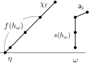
$\underset{1:1}{\overset{\varphi}{\longleftrightarrow}}$

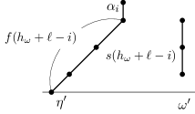
Figure  4: how the involution $\varphi$ works in the proof of Lemma 3.3.

Figure 4 illustrates how the involution $\varphi$ in the proof of Lemma 3.3 changes the paths. The figure represents the beginning part of the paths $\eta$ and $\omega$ where $(\eta,\omega)\in I(n,k)\setminus J(n,k)$. When we are In Case 1, the path’s beginning parts are like the figure’s left side. The involution $\varphi$ changes them to the right side while leaving the remaining parts unchanged.

Lemma 3.4.

Let $\mathcal{L}$ be the linear functional defined by the moments (107). For any non-negative integer $n\in\mathbb{N}_{0}$ and integer $k\in\mathbb{Z}$, we have

2 & ∑_η∈F_n,η starts with α_ℓ,wd(η)=ℓk w(η),    if $$k<n k\geq n$$,
(-1)^n ∑_ω:dual ℓ-Schröderfrom (0,n)to (ℓk-n,0) w(ω), if ,

where $[x^{\leq 0}]P_{n}(x)x^{-\ell k}$ denotes the sum of terms of degree equal to or less than zero in the Laurent polynomial $P_{n}(x)x^{-\ell k}$. The sum (115) on the right-hand side is taken over all Favard paths in $\mathcal{F}_{n}$ whose first steps are $\alpha_{\ell}$ and whose widths are $\ell k$. The sum (115) is taken over all dual $\ell$-Schröder paths from $(0,n)$ to $(\ell k-n,0)$.

Proof.

The left-hand side of the equation (115) can be written as

$$\mathcal{L}\left[[x^{\leq 0}]P_{n}(x)x^{-\ell k}\right]=\sum_{(\eta,\omega)\in\widetilde{I}(n,k)}w(\eta)w(\omega)(-1)^{\operatorname{wd}(\eta)\bmod\ell},$$ (116)

where

$$\widetilde{I}(n,k)\triangleq\{(\eta,\omega)\mid\eta\in\mathcal{F}_{n},\ \operatorname{wd}(\eta)\leq\ell k,\ \omega\in\widetilde{B}_{\ell k-\operatorname{wd}(\eta)}\}.$$ (117)

Let $q$ and $r$ be the quotient and the remainder of dividing $h$ by $\ell$. We define the dual-Favard prefix $F(h)$ as the path from $(0,-\ell+1)$ with $F(h)\triangleq\alpha_{\ell}^{q}$ if $r=0$ and $F(h)\triangleq\chi_{r}\alpha_{\ell}^{q}$ if $r>0$. Also, define the dual-Schröder prefix $S(h)$ as the path from $(0,r)$ with steps $S(h)\triangleq\mathsf{A}_{0}^{q}$.

Define subsets $\widetilde{J}_{1}(n,k),\widetilde{J}_{2}(n,k)$ and $\widetilde{J}(n,k)$ of $\widetilde{I}(n,k)$ as

$$\widetilde{J}_{1}(n,k) \triangleq\{(\eta,\varepsilon)\mid\eta\in\mathcal{F}_{n},\ {\rm the\ first\ step\ of\ }\eta{\rm\ is\ }\alpha_{\ell},\operatorname{wd}(\eta)=\ell k\},$$ (118)

$$\widetilde{J}_{2}(n,k) \triangleq\{(F(n),S(n)\omega^{\prime})\mid\text{$\omega^{\prime}$ is a dual $\ell$-Schr\"{o}der path,\ }S(n)\omega^{\prime}\in\widetilde{\mathcal{B}}_{\ell k-r}\},$$ (119)

and $\widetilde{J}(n,k)\triangleq\widetilde{J}_{1}(n,k)\cup J_{2}(n,k)$. The right-hand side of (115) is the weighted sum over $\widetilde{J}(n,k)$ since when $n\neq 0$, we have $\widetilde{J}_{1}(n,k)=\emptyset$ if $k\geq n$ and $\widetilde{J}_{2}(n,k)=\emptyset$ if $k<n$.

For any $(\eta,\omega)\in\widetilde{I}(n,k)\setminus\widetilde{J}(n,k)$, let $h_{\eta}$ (resp. $h_{\omega}$) be the maximum integer such that $\eta=F(h_{\eta})\eta_{1}$ for some paht $\eta_{1}$ (resp. $\omega=S(h_{\omega})\omega_{1}$ for some path $\omega_{1}$). Let us define a sign-reversing involution $\widetilde{\varphi}$ on the set $\widetilde{I}(n,k)\setminus\widetilde{J}(n,k)$, similar to that in Lemma 3.3. It compares the values $h_{\eta}$ and $h_{\omega}$.

Case 1: When $h_{\eta}>h_{\omega}$.

We can write $\eta$ and $\omega$ as $\eta=F(h_{\omega})\eta_{1}$ and $\omega=S(h_{\omega})\omega_{1}$ using some path $\eta_{1}$ and $\omega_{1}$. Then $\omega_{1}\neq\varepsilon$ since $(\eta,\omega)\notin\widetilde{J}_{1}(n,k)$. The first step of $\omega_{1}$ is $\mathsf{A}_{i}$ for some $i\in\{1,\ldots,\ell+1\}$ because of the maximality of $h_{\omega}$. Also, the first step of $\eta_{1}$ is $\alpha_{\ell}$ because of the maximality of $h_{\eta}$ and $h_{\eta}>h_{\omega}$. Thus we can write $(\eta,\omega)$ as $(\eta,\omega)=(F(h_{\omega})\alpha_{\ell}\eta_{2},s(h_{\omega})\mathsf{A}_{i}\omega_{2})$ for some paths $\eta_{2}$ and $\omega_{2}$. Define the value of $\widetilde{\varphi}$ as

$$\widetilde{\varphi}(\eta,\omega)\triangleq\left\{\begin{array}[]{ll}(F(h_{\omega})\chi_{\ell}\eta_{2},S(h_{\omega})\omega_{2}),&{\rm if}\ i=\ell,\\ (F(h_{\eta}+\ell-i)\alpha_{i}\eta_{2},S(h_{\eta}+\ell-i)\omega_{2}),&{\rm if}\ i\neq\ell.\end{array}\right.$$ (122)

Case 2: When $h_{\eta}\leq h_{\omega}$.

Write as $\eta=F(h_{\eta})\eta_{1}$ and $\omega=S(h_{\eta})\omega_{1}$. Then $\eta_{1}\neq\varepsilon$ since $(\eta,\omega)\notin\widetilde{J}_{2}(n,k)$, hence let the first step of $\eta_{1}$ be $\sigma$. From the maximality of $h_{\eta}$, we have $\sigma\neq\alpha_{\ell}$, that is, $\sigma\in\{\alpha_{1},\alpha_{2},\ldots,\alpha_{\ell-1},\alpha_{\ell+1},\chi_{\ell}\}$. We can write $(\eta,\omega)$ as $(\eta,\omega)=(F(h_{\omega})\sigma\eta_{2},S(h_{\eta})\omega_{1})$. Define the value of $\widetilde{\varphi}$ as

$$\widetilde{\varphi}(\eta,\omega)\triangleq\left\{\begin{array}[]{ll}(F(h_{\eta})\alpha_{\ell}\eta_{2},S(h_{\eta})\mathsf{A}_{\ell}\omega_{1}),&{\rm if}\ \sigma=\chi_{\ell},\\ (F(h_{\eta}+i-\ell)\alpha_{\ell}\eta_{2},S(h_{\eta}+i-\ell)\mathsf{A}_{i}\omega_{1}),&{\rm if}\ \sigma=\alpha_{i}\ {\rm for\ some\ }i\neq\ell.\end{array}\right.$$ (125)

Let $(\eta^{\ast},\omega^{\ast})\triangleq\widetilde{\varphi}(\eta,\omega)$. We show $\widetilde{\varphi}(\eta,\omega)\in\widetilde{I}(n,k)\setminus\widetilde{J}(n,k)$ by showing

$$\operatorname{wd}(\eta)+\operatorname{wd}(\omega)=\operatorname{wd}(\eta^{\ast})+\operatorname{wd}(\omega^{\ast}).$$ (126)

If (126) holds, then from $\omega\in\widetilde{\mathcal{B}}_{\ell k-\operatorname{wd}(\eta)}$, we have $\operatorname{wd}(\omega^{\ast})=\ell k-\operatorname{wd}(\eta^{\ast})$ and from $\operatorname{wd}(\omega^{\ast})\geq 0$, we have $\ell k\geq\operatorname{wd}(\eta^{\ast})$; Thus we have $(\eta^{\ast},\omega^{\ast})\in\widetilde{I}(n,k)$ if (126) holds. The proof of (126) is the following. When in Case 1 and when $(\eta,\omega)=(F(h_{\omega})\alpha_{\ell}\eta_{2},S(h_{\omega})\mathsf{A}_{\ell}\omega_{2})$, we have

$$\left\{\begin{array}[]{l}\operatorname{wd}(\eta)=r+\operatorname{wd}(\eta_{2}),\\ \operatorname{wd}(\omega)=\ell q+\ell+\operatorname{wd}(\omega_{2}),\end{array}\right.\ {\rm and}\ \left\{\begin{array}[]{l}\operatorname{wd}(\eta^{\ast})=r+\ell+\operatorname{wd}(\eta_{2}),\\ \operatorname{wd}(\omega^{\ast})=\ell q+\operatorname{wd}(\omega_{2}),\end{array}\right.$$ (131)

where the quotient and the remainder of dividing $h_{\omega}$ by $\ell$ are denoted as $q$ and $r$, respectively, hence (126) holds. A similar proof works for the remaining cases. It is easy to check that $\widetilde{\varphi}$ is an involution. The remaining task is to check $\widetilde{\varphi}$ is sign-reversing. When in Case 1 and when $(\eta,\omega)=(F(h_{\omega})\alpha_{\ell}\eta_{2},S(h_{\omega})\mathsf{A}_{\ell}\omega_{2})$, it suffices to show that

$$w(F(h_{\omega})\alpha_{\ell})w(S(h_{\omega})\mathsf{A}_{\ell})=-w(F(h_{\omega})\chi_{\ell})w(S(h_{\omega})).$$ (132)

By substituting

$$w(F(h_{\omega})\alpha_{\ell}) =\left(\prod_{j=0}^{q-1}(-a_{\ell,r+j\ell})\right)(-a_{\ell,h_{\omega}}),$$ (133)

$$w(S(h_{\omega})\mathsf{A}_{\ell}) =\left(\prod_{j=0}^{q-1}\frac{(-1)^{\ell+1}}{a_{\ell,r+j\ell}}\right)\frac{1}{a_{\ell,h_{\omega}}},$$ (134)

$$w(F(h_{\omega})\chi_{\ell}) =\left(\prod_{j=0}^{q-1}(-a_{\ell,r+j\ell})\right),\quad\textrm{and}$$ (135)

$$w(S(h_{\omega})) =\left(\prod_{j=0}^{q-1}\frac{(-1)^{\ell+1}}{a_{\ell,r+j\ell}}\right),$$ (136)

one can check that (132) holds. When $(\eta,\omega)=(F(h_{\omega})\alpha_{\ell}\eta_{2},S(h_{\omega})\mathsf{A}_{i}\omega_{2})$ for $i\neq\ell$, let us write $q^{\ast}$ and $r^{\ast}$ the quotient and the remainder of dividing $h_{\omega}+\ell-i$ by $\ell$, respectively. It suffices to show that

$$w(F(h_{\omega})\alpha_{\ell})w(S(h_{\omega})\mathsf{A}_{i})(-1)^{r}=-w(F(h_{\omega}+\ell-i)\alpha_{\ell})w(S(h_{\omega}+\ell-i))(-1)^{r^{\ast}}.$$ (137)

By substituting

$$w(S(h_{\omega})\mathsf{A}_{i}) =\left(\prod_{j=0}^{q-1}\frac{(-1)^{\ell+1}}{a_{\ell,r+j\ell}}\right)\frac{(-1)^{\ell+1+i}a_{i,h_{\omega}}}{a_{\ell},h_{\omega}},$$ (139)

$$w(F(h_{\omega}+\ell-i)\alpha_{i}) =\left(\prod_{j=0}^{q^{\ast}-1}(-a_{\ell,r^{\ast}+j\ell})\right)(-a_{i,h_{\omega}}),$$ (140)

$$w(S(h_{\omega}+\ell-i)) =\prod_{j=0}^{q^{\ast}-1}\frac{(-1)^{\ell+1}}{a_{\ell,r^{\ast}-j\ell}},$$ (141)

and (133), one can check that (LABEL:eq:wwww3) holds. A similar proof works for Case2. ∎

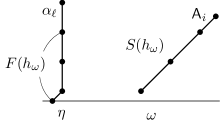
$\underset{1:1}{\overset{\widetilde{\varphi}}{\longleftrightarrow}}$

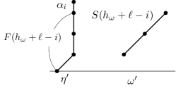
Figure  5: how the involution $\widetilde{\varphi}$ works in the proof of Lemma 3.4.

Figure 5 illustrates how the involution $\widetilde{\varphi}$ in the proof of Lemma 3.4 changes the paths. In Case 1, the beginning parts of the paths are like the left side. The involution $\widetilde{\varphi}$ changes them as the right side while leaving the remaining parts unchanged.

Combining Lemma 3.3 and Lemma 3.4, we obtain the general orthogonality.

Theorem 3.5.

Let $\mathcal{L}$ be the linear functional defined by the moments (107). For any non-negative integer $n\in\mathbb{N}_{0}$ and integer $k\in\mathbb{Z}$, we have

2 & (-1)^n ∑_ω:dual ℓ-Schröderfrom (0,n)to (ℓk-n,0) w(ω),    if $$n\leq k 0\leq k\leq n-1 k<0$$,
0,if ,
a_ℓ,0 ∑_ω:ℓ-Schröderfrom (0,n) to (n-ℓ(k+1),0)w(ω), if .

More specifically, we have

$$\mathcal{L}[P_{n}(x)x^{-n\ell}]=(-1)^{n}\prod_{i=1}^{n}\frac{a_{\ell+1,i}}{a_{\ell,i}}$$ (143)

when $k=n$, and

$$\mathcal{L}[P_{n}(x)x^{\ell}]=a_{\ell,0}\prod_{i=1}^{n}a_{\ell+1,i}$$ (144)

when $k=-1$.

Proof.

Substitute (108) and (115) into

$$\mathcal{L}[P_{n}(x)x^{-\ell k}]=\mathcal{L}[[x^{>0}]P_{n}(x)x^{-\ell k}]+\mathcal{L}[[x^{\leq 0}]P_{n}(x)x^{-\ell k}].$$ (145)

We get (142) since $\mathcal{L}[[x^{>0}]P_{n}(x)x^{-\ell k}]=0$ if $n\leq k$, get (142) since $\mathcal{L}[[x^{\leq 0}]P_{n}(x)x^{-\ell k}]=0$ if $k<0$, and (142) since $\mathcal{L}[[x^{>0}]P_{n}(x)x^{-\ell k}]+\mathcal{L}[[x^{\leq 0}]P_{n}(x)x^{-\ell k}]=0$ if $0\leq k\leq n-1$. When $k=n$, the right-hand side of (142) is the weight of the pair $(\eta,\omega)=(F(n),S(n)\mathsf{A}_{\ell+1}^{n})$. When $k=-1$, the right-hand side is the wheigh of $(\eta,\omega)=(f(n),s(n)\mathsf{a}_{\ell+1}^{n})$. ∎

4 Non-intersecting tuplets of $\ell$-Schröder paths

In the latter half of this paper, we study enumerative aspects of $\ell$-Schröder paths and new paths called small $\ell$-Schröder paths. The results are applied to obtain closed-form generating functions for non-intersecting tuplets of $\ell$-Schröder paths, the second aim of this paper.

Before we get to the main point, we would like to briefly discuss Narayana polynomials to relate the results of this chapter to the $\ell$-LBPs. Recall that the conventional Narayana polynomials [12, 2] are the generating functions of Schröder paths concerning the number of steps $(2,0)$. We define the $n$-th $\ell$-Narayana polynomial $N_{n}(a_{1},\ldots,a_{\ell+1})$ as

$$N_{n}=N_{n}(a_{1},\ldots,a_{\ell+1})\triangleq\sum_{\omega\in\mathcal{B}_{n}}\prod_{i=1}^{\ell+1}a_{i}^{(\text{number of steps $\mathsf{a_{i}}$ in $\omega$})}.$$ (146)

The moments of positive degrees of primitive $\ell$-LBPs are written by $\ell$-Narayana polynomials as $\mu_{n+\ell}=a_{\ell}N_{n}\ (n\geq 0)$ when the recurrence coefficients in (2) are constants as $a_{i,j}\triangleq a_{i}$ for all $i=1,\ldots,\ell+1$ and $j\in\mathbb{N}_{0}$. Using the results of this chapter, we will show the following two property of $\ell$-Narayana polynomials.

Theorem 4.1.

For any integer $n\geq\ell$, the $n$-th $\ell$-Narayana polynomial is divisible by $\sum_{i=0}^{\ell}a_{i}a_{\ell+1}^{\ell-i}$, where $a_{0}\triangleq 1$.

Theorem 4.2.

The following block Hankel determinant of $\ell$-Narayana polynomials can be factorized as

$$\det(N_{\ell(i+1)+j})_{i,j=0}^{n-1}=a_{\ell+1}^{\binom{n}{2}}\left(\sum_{i=0}^{\ell}a_{i}a_{\ell+1}^{\ell-i}\right)^{\binom{n+1}{2}},$$ (147)

where $a_{0}\triangleq 1$.

Remark 4.1.

Theorem 4.1 reduces to Proposition 2.1 in [2] when $\ell=1$, which describes roots of Narayana polynomials.

4.1 Relation between big and small $\ell$-Schröder paths

We introduce two new paths and consider their relations with $\ell$-Schröder paths. Firstly, let us define a new weight $v$ on $\ell$-Schröder paths, more suitable for the aim of this chapter. The weight of the step $\mathsf{a}_{i}\ (0\leq i\leq\ell)$ from the point $(x,y)\in\mathbb{Z}^{2}$ is defined as $v(\mathsf{a}_{i},(x,y))\triangleq b_{i,j}$, and the weight of $\mathsf{a}_{\ell+1}$ from $(x,y)$ is defined as $v(\mathsf{a}_{\ell+1},(x,y))\triangleq c_{j}$, where $j\triangleq(x+y)/\ell$.

Let us denote by $\mathcal{B}_{s,t}^{r}$ the set of $\ell$-Schröder paths from $(s\ell-r,r)$ to $(t\ell,0)$. The generating function for the set $\mathcal{B}_{s,t}^{r}$ is denoted by $v(\mathcal{B}_{s,t}^{r})\triangleq\sum_{\omega\in\mathcal{B}_{s,t}^{r}}v(\omega)$.

A small $\ell$-Schröder path is an $\ell$-Schröder path that does not have any step $\mathsf{a}_{i}$ starting from in the region $y\leq i-1$ for all $i=1,\ldots,\ell$. Let us denote by $\mathcal{S}_{s,t}^{r}$ the set of small $\ell$-Schröder paths from $(s\ell-r,r)$ to $(t\ell,0)$. We refer to $\ell$-Schörder paths as big $\ell$-Schröder paths. A marked $\ell$-Schröder path is a big $\ell$-Schröder path with a mark on its eastern slope, that is, an element of the set

$$\mathcal{M}_{s,t}^{r}\triangleq\{(\omega,m)\in\mathcal{B}_{s,t}^{r}\times\mathbb{N}_{0}\mid\omega\textrm{ have a step starting or ending at }(t\ell-m,m)\},$$ (148)

if $s\neq t$ or $r>0$, and $\mathcal{M}_{t,t}^{0}\triangleq\{(\varepsilon,0)\}$, if $s=t$ and $r=0$. See Fugire 7 for examples of marked (left-side) and small (right-side) $\ell$-Schröder paths.

A weight $v$ of marked $\ell$-Schröder paths is defined as, for $(\omega,m)\in\mathcal{M}_{s,t}^{r}$,

$$v((\omega,m))\triangleq v(\omega)\frac{c_{t+1}^{m}}{c_{t}^{m}}.$$ (149)

The generating functions of $\mathcal{S}_{s,t}^{r}$ and $\mathcal{M}_{s,t}^{r}$ are denoted by $v(\mathcal{S}_{s,t}^{r})\triangleq\sum_{\omega\in\mathcal{S}_{s,t}^{r}}v(\omega)$ and $v(\mathcal{M}_{s,t}^{r})\triangleq\sum_{(\omega,m)\in\mathcal{M}_{s,t}^{r}}v((\omega,m))$, respectively. The following lemmas describe the relation between generating functions $v(\mathcal{B}_{s,t}^{r})$, $v(\mathcal{S}_{s,t}^{r})$ and $v(\mathcal{M}_{s,t}^{r})$.

Lemma 4.3.

For any integers $s,t$ with $s\leq t$ and non-negative integer $r$ with $0\leq r<\ell$, we have

$$v(\mathcal{B}_{s,t+1}^{r})=v(\mathcal{M}_{s,t}^{r})\sum_{i=0}^{\ell}b_{i,t}c_{t+1}^{\ell-i}.$$ (150)

Proof.

The proof is based on a weight-preserving bijection $\theta\colon\mathcal{B}_{s,t+1}^{r}\to\mathcal{M}_{s,t}^{r}\times\mathcal{B}_{t,t+1}^{0}$. The map $\theta$ is defined as follows. Let $\omega\in\mathcal{B}_{s,t+1}^{r}$. Tracing the path $\omega$ backward from the final step, there is a step $\mathsf{a}_{\ell-k}$ other than $\mathsf{a}_{\ell+1}$ that is encountered first. Hence we can write uniquely as $\omega=\omega_{1}\mathsf{a}_{\ell-k}\mathsf{a}_{\ell+1}^{k+m}$ for some path $\omega_{1}$ and non-negative integers $m,k$. Define $\theta$ as $\theta(\omega)\triangleq((\omega_{1}\mathsf{a}_{\ell}^{m},m),\mathsf{a}_{\ell-k}\mathsf{a}_{\ell+1}^{k})\in\mathcal{M}_{s,t}^{r}\times\mathcal{B}_{t,t+1}^{0}$. ∎

$\overset{\theta}{\underset{1:1}{\longrightarrow}}$

Figure  6: Left: a big $3$-Schröder path $\omega\in\mathcal{B}_{0,5}^{1}$. Right: the pair $\theta(\omega)=((\omega^{\prime},m),\omega^{\prime\prime})\in\mathcal{M}_{0,4}^{1}\times\mathcal{B}_{4,5}^{0}$

Figure 6 shows how the bijection $\theta$ in Lemma 4.3 works. The left side is a big $3$-Schröder path $\omega\in\mathcal{B}_{0,5}^{1}$ with steps $\omega=\mathsf{a}_{1}\mathsf{a}_{4}^{2}\mathsf{a}_{3}\mathsf{a}_{4}\mathsf{a}_{2}\mathsf{a}_{1}\mathsf{a}_{4}^{3}$. The right side is a pair $((\omega^{\prime},m),\omega^{\prime\prime})$ of a marked $3$-Schröder path $(\omega^{\prime},m)\in\mathcal{M}_{0,4}^{1}$ and a big $3$-Schroder path $\omega^{\prime\prime}\in\mathcal{B}_{4,5}^{0}$, where the steps are $\omega^{\prime}=\mathsf{a}_{1}\mathsf{a}_{4}^{2}\mathsf{a}_{3}\mathsf{a}_{4}\mathsf{a}_{2}\mathsf{a}_{4}$, $\omega^{\prime\prime}=\mathsf{a}_{1}\mathsf{a}_{4}^{2}$. and $m=1$. The bijection $\theta$ maps $\omega$ onto $((\omega^{\prime},m),\omega^{\prime\prime})$.

Lemma 4.4.

For any integers $s,t$ with $s\leq t$ and non-negative integer $r$ with $0\leq r<\ell$, we have

$$v(\mathcal{M}_{s,t}^{r})=c_{t+1}^{-\ell}\sum_{i=0}^{r}c_{s}^{r-i}\left(v(\mathcal{S}_{s,t}^{i+\ell})\mid_{c_{k}:=c_{k+1}}\right).$$ (151)

The symbol $v(\mathcal{S}_{s,t}^{i+\ell})|_{c_{k}:=c_{k+1}}$ in (151) represents the generating function $v(\mathcal{S}_{s,t}^{i+\ell})$ in which all the variables $c_{k}$ replaced by the variable $c_{k+1}$ simultaneously for all $k\in\mathbb{Z}$.

Proof.

The statement is obvious if $s=t$. Let us consider the case when $s<t$. We decompose the set $\mathcal{M}_{s,t}^{r}$ into $r+1$ disjoint subsets based on the number of steps $\mathsf{a}_{\ell+1}$ placed at the beginning of paths. Let $\mathcal{N}_{s,t}^{r}$ be the subset of $\mathcal{M}_{s,t}^{r}$ defined as

$$\mathcal{N}_{s,t}^{r}\triangleq\{(\omega,m)\mid(\omega,m)\in\mathcal{M}_{s,t}^{r},\ {\rm the\ first\ step\ of\ }\omega{\rm\ is\ not\ }\mathsf{a}_{\ell+1}\}.$$ (152)

Using $\mathcal{N}_{s,t}^{r}$, the set $\mathcal{M}_{s,t}^{r}$ can be decomposed as

$$\mathcal{M}_{s,t}^{r}=\bigsqcup_{i=0}^{r}\mathsf{a}_{\ell+1}^{r-i}\mathcal{N}_{s,t}^{i},$$ (153)

where $\mathsf{a}_{\ell+1}^{r-i}\mathcal{N}_{s,t}^{i}$ denotes the set of marked $\ell$-Schröder paths in $\mathcal{M}_{s,t}^{r}$ whose first $r-i$ steps are $\mathsf{a}_{\ell+1}$ and $(r-i+1)$-th step is not $\mathsf{a}_{\ell+1}$. From (153), writing the generating function of $\mathcal{N}_{s,t}^{r}$ as $v(\mathcal{N}_{s,t}^{r})\triangleq\sum_{(\omega,m)\in\mathcal{N}_{s,t}^{r}}v((\omega,m))$, we have

$$v(\mathcal{M}_{s,t}^{r})=\sum_{i=0}^{r}c_{s}^{r-i}v(\mathcal{N}_{s,t}^{i}).$$ (154)

Our next step is to construct a bijection that sends $(\omega,m)\in\mathcal{N}_{s,t}^{i}$ to $\omega^{\prime}\in\mathcal{S}_{s,t}^{i+\ell}$ for $0\leq i\leq r$ that satisfies

$$v((\omega,m))=\left.\left(\frac{1}{c_{t}^{\ell}}v(\omega^{\prime})\right)\middle|_{c_{k}:=c_{k+1}}\right..$$ (155)

If such a bijection exists, then by summing (155) over $\mathcal{N}_{s,t}^{r}$ we have

$$v(\mathcal{N}_{s,t}^{i})=c_{t+1}^{-\ell}\left(v(\mathcal{S}_{s,t}^{i+\ell})\mid_{c_{k}:=c_{k+1}}\right)$$ (156)

and, together with (154), we get (151). The bijection is constructed as follows.

We split the marked path $(\omega,m)\in\mathcal{N}_{s,t}^{i}$ into two paths, before and after the mark. The former is a path from $(s\ell-i,i)$ to $(t\ell-m,m)$, and the latter is a path from $(t\ell-m,m)$ to $(t\ell,0)$. Let us denote the former as $\omega_{1}$ and the latter as $\omega_{2}$. The path $\omega_{1}$ has a unique decomposition as a sequence of the elements of $\{\mathsf{a}_{j}\mathsf{a}_{\ell+1}^{k}\mid 0\leq j\leq\ell,k\geq 0\}$. Let us write this decomposition as $\omega_{1}=\alpha_{1}\cdots\alpha_{d}$. We define $\omega^{\prime}$ as the path from $(s\ell-i-\ell,i+\ell)$ with steps

$$\omega^{\prime}\triangleq\operatorname{rot}(\alpha_{1})\cdots\operatorname{rot}(\alpha_{d})\omega_{2}\mathsf{a}_{\ell+1}^{\ell},$$ (157)

where $\operatorname{rot}(v_{1}v_{2}\cdots v_{n})\triangleq v_{2}\cdots v_{n}v_{1}$. This map $\mathcal{N}_{s,t}^{i}\ni(\omega,m)\mapsto\omega^{\prime}\in\mathcal{S}_{s,t}^{i+\ell}$ is a bijection and it satisfies (155). ∎

$\underset{1:1}{\longrightarrow}$

Figure  7: Left: a marked $3$-Schröder path in $\mathcal{N}_{0,4}^{1}$. Right: a small $3$-Schröder path in $\mathcal{S}_{0,4}^{4}$.

Figure 7 shows an example of how the bijection in Lemma 4.4 works. The left side is a marked $3$-Schröder path $(\omega,1)\in\mathcal{N}_{0,4}^{1}$ with steps $\omega=\mathsf{a}_{1}\mathsf{a}_{4}^{2}\mathsf{a}_{3}\mathsf{a}_{4}\mathsf{a}_{2}\mathsf{a}_{4}$. The decomposition of $\omega$ is as $\omega=(\mathsf{a}_{1}\mathsf{a}_{4}^{2})(\mathsf{a}_{3}\mathsf{a}_{4})(\mathsf{a}_{2})\mathsf{a}_{4}$. Therefore, the bijection maps $(\omega,1)$ onto the small $3$-Schröder paths $\omega^{\prime}\in\mathcal{S}_{0,4}^{4}$ on the right side of the figure. The steps of $\omega^{\prime}$ are $\omega^{\prime}=\mathsf{a}_{4}^{2}\mathsf{a}_{1}\mathsf{a}_{4}\mathsf{a}_{3}\mathsf{a}_{2}\mathsf{a}_{4}^{4}$.

Combining Lemma 4.3 and Lemma 4.4, we obtain the following.

Theorem 4.5.

For any integers $s,t$ with $s\leq t$ and non-negative integer $r$ with $0\leq r<\ell$, we have

$$v(\mathcal{B}_{s,{t+1}}^{r})=c_{t+1}^{-\ell}\left(\sum_{i=0}^{r}c_{s}^{r-i}\left(v(\mathcal{S}_{s,t}^{i+\ell})\middle|_{c_{k}:=c_{k+1}}\right)\right)\left(\sum_{i=0}^{\ell}b_{i,t}c_{t+1}^{\ell-i}\right).$$ (158)

We obtain Theorem 4.1 mentioned at the beginning of the chapter by setting the variables in Theorem 4.5 as $b_{i,j}:=a_{i}$ for $i=0,\ldots,\ell+1$ and $c_{j}:=a_{\ell+1}$. Also by $b_{i,j}:=1$ and $c_{j}:=1$ for all $i,j\in\mathbb{Z}$ in Theorem 4.5, we obtain the following.

Corollary 4.6.

For any integers $s,t$ with $s\leq t$ and non-negative integer $r$ with $0\leq r<\ell$, we have

$$|\mathcal{B}_{s,t+1}^{r}|=(\ell+1)\sum_{i=0}^{r}|\mathcal{S}_{s,t}^{i+\ell}|.$$ (159)

Corollary 4.6 is reduced to the well-known fact that the $n$-th big Schröder number is double the $n$-th small Schröder number when $\ell=1$ (cf. [19]).

4.2 Generating functions for non-intersecting tuplets of $\ell$-Schröder paths

In this subsection, we show that some generating functions of non-intersecting tuplets of $\ell$-Schröder paths are factorized nicely, as in the case of $\ell=1$. We generalize the technique developed by Eu and Fu [7] for Schröder paths. Theorem 4.5 plays an essential role in the proof of the factorization.

Let us define some terms that we need for non-intersecting paths. Let $\mathbf{s}=(s_{0},\ldots,s_{n-1})$ and $\mathbf{t}=(t_{0},\ldots,t_{n-1})$ be tuplets of points in $\mathbb{Z}^{2}$. A path system of size $n$ from $\mathbf{s}$ to $\mathbf{t}$ is a tuplet of paths $(\omega_{0},\ldots,\omega_{n-1})$ such that $\omega_{i}$ is from $s_{i}$ to $t_{\sigma(i)}$ for $0\leq i\leq n-1$, where $\sigma$ is a permutation on $\{0,1,\ldots,n-1\}$. A path system is said to be non-intersecting if the paths are pairwise disjoint, i.e., if no steps in the paths share their starting or ending point. The weight $v(\boldsymbol{\omega})$ of a path system $\boldsymbol{\omega}=(\omega_{0},\ldots,\omega_{n-1})$ is defined as $v(\boldsymbol{\omega})\triangleq\operatorname{sign}(\sigma)v(\omega_{0})\cdots v(\omega_{n-1})$.

Let us denote as $\Pi_{n}$ the set of non-intersecting path systems of $n$ $\ell$-Schröder paths from $\mathbf{s}$ to $\mathbf{t}$ with

$$\mathbf{s} \triangleq((-i,i\bmod\ell))_{i=0,\ldots,n-1}\qquad\textrm{and}$$ (160)

$$\mathbf{t} \triangleq(((i+1)\ell,0))_{i=0,\ldots,n-1},$$ (161)

where $i\bmod\ell$ denotes the remainder of dividing $i$ by $\ell$. Also, denote as $\Omega_{n}$ the set of non-intersecting systems of $n$ small $\ell$-Schröder paths from $\mathbf{s}$ to $\mathbf{t}$ with

$$\mathbf{s} \triangleq((-i,(i\bmod\ell)+\ell))_{i=0,\ldots,n-1}\qquad\textrm{and}$$ (162)

$$\mathbf{t} \triangleq((i\ell,0))_{i=0,\ldots,n-1}.$$ (163)

See Figure 8 for examples of non-intersecting paths in $\Pi_{n}$ (left side) and $\Omega_{n}$ (right side). Note that although a path system is non-intersecting, lines may cross when drawn in a plane.

Let us write the generating function of $\Pi_{n}$ and $\Omega_{n}$ as

$$v(\Pi_{n})\triangleq\sum_{\boldsymbol{\omega}\in\Pi_{n}}v(\boldsymbol{\omega}),\qquad v(\Omega_{n})\triangleq\sum_{\boldsymbol{\omega}\in\Omega_{n}}v(\boldsymbol{\omega}).$$ (164)

These generating functions have the following relations.

Lemma 4.7.

For any non-negative integer $n$, we have

$$v(\Pi_{n})=\left(v(\Omega_{n})\middle|_{c_{k}:=c_{k+1}}\right)\times\prod_{t=0}^{n-1}\left(c_{t+1}^{-\ell}\sum_{i=0}^{\ell}b_{i,t}c_{t+1}^{\ell-i}\right).$$ (165)

Proof.

From the Lindström–Gessel–Viennot lemma [9], we know that $v(\Pi_{n})$ and $v(\Omega_{n})$ are written as determinants of generating functions of big and small $\ell$-Schröder paths as

$$v(\Pi_{n}) =\det(v(\mathcal{B}_{-\lfloor i/\ell\rfloor,j+1}^{i\bmod\ell}))_{i,j=0}^{n-1},$$ (166)

$$v(\Omega_{n}) =\det(v(\mathcal{S}_{-\lfloor i/\ell\rfloor,j}^{(i\bmod\ell)+\ell}))_{i,j=0}^{n-1},$$ (167)

where $\lfloor i/\ell\rfloor$ and $i\bmod\ell$ denotes the quotient and the remainder of $i$ divided by $\ell$. Substituting (158) into (166), we have

$$\begin{aligned} &\det(v(\mathcal{B}_{-\lfloor i/\ell\rfloor,j+1}^{i\bmod\ell}))_{i,j=0}^{n-1}\\ &=\left(\prod_{t=0}^{n-1}c_{t+1}^{-\ell}\sum_{i=0}^{\ell}b_{i,t}c_{t+1}^{\ell-i}\right)\det\left(\sum_{p=0}^{i\bmod\ell}c_{-\lfloor i/\ell\rfloor}^{(i\bmod\ell)-p}\left(v(\mathcal{S}_{-\lfloor i/\ell\rfloor,j}^{p+\ell})\middle|_{c_{k}:=c_{k+1}}\right)\right)_{i,j=0}^{n-1}.\end{aligned}$$ (168)

By performing the elementary row operations on the determinant in (168), we obtain

$$\det(v(\mathcal{B}_{-\lfloor i/\ell\rfloor,j+1}^{i\bmod\ell}))_{i,j=0}^{n-1}=\left(\prod_{t=0}^{n-1}c_{t+1}^{-\ell}\sum_{i=0}^{\ell}b_{i,t}c_{t+1}^{\ell-i}\right)\det\left(v(\mathcal{S}_{\lfloor i/\ell\rfloor,j}^{(i\bmod\ell)+\ell})|_{c_{k}:=c_{k+1}}\right)_{i,j=0}^{n-1}.$$ (169)

From (169) and (167), we obtain (165). ∎

The generating functions also satisfy the following.

Lemma 4.8.

For any positive integer $n$, we have

$$v(\Omega_{n})=c_{0}^{\ell}\left(\prod_{i=1}^{n-1}c_{i}^{\ell+1}\right)\left(\prod_{i=1}^{\lfloor(n-1)/\ell\rfloor}b_{0,-i}\right)v(\Pi_{n-1}).$$ (170)

Proof.

There is a natural bijection between $\Pi_{n-1}$ and $\Omega_{n}$ that shift all paths in $\boldsymbol{\omega}\in\Pi_{n-1}$ northwestward. Let $\boldsymbol{\omega}=(\omega_{0},\ldots,\omega_{n-2})\in\Pi_{n-1}$. The bijection is defined as $\boldsymbol{\omega}\mapsto\boldsymbol{\omega}^{\prime}\triangleq(\mathsf{a}_{\ell+1}^{\ell},\omega_{0}^{\prime},\ldots,\omega_{n-2}^{\prime})\in\Omega_{n}$ where the word for $\omega^{\prime}_{i}$ is defined as

$$\omega_{i}^{\prime}\triangleq\left\{\begin{array}[]{ll}\omega_{i}\mathsf{a}_{\ell+1}^{\ell+1}&{\rm if\ }i\bmod\ell\not\equiv\ell-1,\\ \mathsf{a}_{0}\omega_{i}\mathsf{a}_{\ell+1}^{\ell+1}&{\rm if\ }i\bmod\ell\equiv\ell-1.\end{array}\right.$$ (173)

The weight $v(\boldsymbol{\omega}^{\prime})$ of the new path system satisfies

$$v(\boldsymbol{\omega}^{\prime})=c_{0}^{\ell}\left(\prod_{i=1}^{n-1}c_{i}^{\ell+1}\right)\left(\prod_{i=1}^{\lfloor(n-1)/\ell\rfloor}b_{0,-i}\right)v(\boldsymbol{\omega}).$$ (174)

Summing up over $\Pi_{n-1}$ leads to (170). Figure 8 shows an example of the bijection. ∎

$\underset{1:1}{\longrightarrow}$

Figure  8: Left: a non-intersecting tuplet of big $3$-Schröder paths in the set $\Pi_{4}$. Right: a non-intersecting tuplet of small $3$-Schröder paths in the set $\Omega_{5}$. The dotted lines are frozen steps due to the non-intersectingness.

Combining Lemma 4.7 and Lemma 4.8, we obtain a recurrence for $v(\Pi_{n})$.

Lemma 4.9.

For any positive integer $n$, we have

$$v(\Pi_{n})=\left(\prod_{i=2}^{n}c_{i}\right)\left(\prod_{i=1}^{\lfloor(n-1)/\ell\rfloor}b_{0,-i}\right)\left(\prod_{t=0}^{n-1}\sum_{i=0}^{\ell}b_{i,t}c_{t+1}^{\ell-i}\right)(v(\Pi_{n-1})|_{c_{k}:=c_{k+1}}).$$ (175)

From the recurrence (175), we have an explicit formula for $v(\Pi_{n})$. This is the main theorem of the latter half of this paper.

Theorem 4.10.

For any non-negative integer $n$, we have

$$v(\Pi_{n})=\left(\prod_{i=2}^{n}c_{i}^{i-1}\prod_{j=1}^{\lfloor(i-1)/\ell\rfloor}b_{0,-j}\right)\left(\prod_{s=1}^{n-1}\prod_{t=0}^{s-1}\sum_{i=0}^{\ell}b_{i,t}c_{s}^{\ell-i}\right).$$ (176)

As a direct consequence of Theorem 4.10, we can show Theorem 4.2 presented at the beginning of the chapter.

Proof of Theorem 4.2.

Reduce the variables appearing in the weight $v$ as $b_{i,j}:=a_{i}$ and $c_{j}:=a_{\ell+1}$ for all $j\in\mathbb{Z}$. Then we have $v(\mathcal{B}^{i\bmod\ell}_{-\lfloor i/\ell\rfloor,j+1})=w(N_{i+\ell(j+1)})$. Thus we have $\det(N_{\ell(i+1)+j})_{i,j=0}^{n-1}=\det(v(\mathcal{B}^{i\bmod\ell}_{-\lfloor i/\ell\rfloor,j+1}))_{i,j=0}^{n-1}=v(\Pi_{n})$. ∎

Remark 4.2.

We obtain Theorem 6.14 in [13] by setting $\ell=2$ in Theorem 4.10. It is worth highlighting that distinct orthogonal functions, namely $R_{I}$ polynomials and $2$-LBPs, result in the same factorization formula.

Remark 4.3.

By considering the one-to-one correspondence between the domino tilings of the Aztec diamonds and the non-intersecting paths in $\Pi_{n}$ when $\ell=1$, one will find that Theorem 4.10 provides another proof of refined Aztec diamond theorem that first appeared in Ciucu [4, Theorem 3.1].

Remark 4.4.

The problem of finding tiling models with a one-to-one correspondence between the non-intersecting paths in $\Pi_{n}$ for $\ell\geq 2$ is still open. It would be interesting to seek such tiling models.

References

- [1] J. Baik, P. Deift, T. Suidan, Combinatorics and random matrix theory. American Mathematical Society, Providence, RI, 2016.
- [2] J.Bonim, L. Shapiro, R. Simion, Some -analogues of the Schröder numbers arising from combinatorial statistics on lattice paths, J. Statist. Plann. Inference 34 (1993) 35–55.
- [3] C. Brezinski, J. Van Iseghem, Vector orthogonal polynomials of dimension , Approximation and computation (West Lafayette, IN, 1993), International Series in Numerical Mathematics, vol. 119, Birkhäuser Boston, Boston, MA, 1994, pp. 29–39.
- [4] M. Ciucu, A complementation theorem for perfect matchings of graphs having a cellular completion, J. Combin. Theory Ser. A 81 (1998) 34–68.
- [5] S. Corteel, J. S. Kim, D. Stanton, Moments of orthogonal polynomials and combinatorics. Recent trends in combinatorics, volume 159 of IMA Vol. Math. Appl., pages 545–578. Springer Cham, 2016.
- [6] N. Elkies, G. Kuperberg, M. Larsen, and J. Propp. Alternating-sign matrices and domino tilings (part I), J. Algebraic Combin. 1 (1992) 111–132.
- [7] S.-P. Eu, T.-S. Fu, A simple proof of the Aztec diamond theorem. Elec. J. Combin., 12 (2005) R18.
- [8] P. D. Francesco, E. Guitter, Twenty-vertex model with domain wall boundaries and domino tilings. Elec. J. Combin., 27(2) (2020) R2.13.
- [9] I. Gessel, G. Viennot, Binomial determinants, paths, and hook legnth formulae, Adv. Math. 58 (1985) 300–321.
- [10] K. Johansson, Non-intersecting paths, random tilings and random matrices, Probab. Theory Related Fields 123 (2002) 225–280.
- [11] S. Kamioka, A combinatorial representation with Schröder paths of biorthogonality of Laurent biorthogonal polynomials, Elec. J. Combin., 14 (2007) R37.
- [12] S. Kamioka, Laurent biotrhogonal polynomials, -Narayana polynomials and domino tilings of the Aztec diamonds, J. Comb. Theory Ser. A 123 (2014) 14–29.
- [13] J. S. Kim, D. Stanton, Combinatorics of orthogonal polynomials of type , Ramanujan J. (2021).
- [14] K. Kobayashi, Studies on discrete integrable systems with positivity and their applications, Ph.D thesis, Kyoto University, Mar. 2022.
- [15] OEIS Foundation Inc. (2023), The On-Line Encyclopedia of Integer Sequences, http://oeis.org.
- [16] V. Strehl, Counting domino tilings of rectangles via resultants, Adv. Appl. Math. 27 (2001) 597–626.
- [17] G. Viennot, A combinatorial theory for general orthogonal polynomials with extensions and applications, in Polynômes Orthogonaux et Applications (Lecture Notes in Mathematics #1171), Springer-Verlag, Berlin, 1985, pp. 139–157.
- [18] B. Wang, X.-K. Chang, X.-L. Yue, A generalization of Laurent biorthogonal polynomials and related integrable lattices, J. Phys. A: Math. Theor. 55 (2022) 214002.
- [19] S.-L. Yang, M.-y. Jiang, The -Schröder paths and -Schröder numbers, Discrete Math. 344 (2021) 112209.
- [20] A. Zhedanov, The “classical” Laurent biorthogonal polynomials, J. comput. appl. math 98.1 (1998) 121–147.