Ordering ambiguity for sharply peaked states in quantum cosmology

Abstract

Sharply peaked quantum states are conjectured to be conducive to the notion of a quantum-corrected spacetime. We investigate this conjecture for a flat-FLRW model with perfect fluid, where a generalized ordering scheme is considered for the gravitational Hamiltonian. We study the implications of different ordering choices on the dynamics of the quantum universe. We demonstrate that the imprints of the operator ordering ambiguity are minimal, and quantum fluctuations are small in the case of sharply peaked states, leading to a consistent notion of a quantum-corrected spacetime defined via the expectation value of scale factor.

1 Introduction

The operator ordering ambiguity is one of the many issues at the heart of all canonical approaches to quantizing gravity Kiefer (2012). Ordering ambiguity in quantum gravity appears in two avatars: the structure of the Hamiltonian constraint involves the product of non-commuting variables leading to inequivalent constraint operator choices DeWitt (1967), and implementation of constraint algebra at the operator level leading to quantum anomalies Tsamis and Woodard (1987). In this work, we will address the first case in the context of a quantum mechanical model of gravity, i.e., a minisuperspace system with finite degrees of freedom. Even in the early seminal work of DeWitt DeWitt (1967), the ordering prescription is proposed for the Hamiltonian constraint, the Laplace-Beltrami ordering, based on physical arguments pertaining to the covariance of the differential operator in the space of 3-geometries Halliwell (1988). However, there is still no consensus on the preferred ordering for the Hamiltonian constraint, and several other choices are also proposed Hawking and Page (1986); Vilenkin (1988b).

The analyses that consider a generalized scheme of the ordering of the Hamiltonian constraint are hard to find; one that deals with how the ordering choice affects the evolution of the quantum universe is further obscure. Still, there are a handful of analyses that address the operator ordering ambiguity at some level, e.g., see Louko (1988); Rostami et al. (2015); Halliwell ; Kontoleon:1998pw ; Bojowald (2002); Bojowald and Simpson (2014); Kiefer and Schmitz (2019); Matsui:2021yte ; Sahota and Lochan (2023, 2021). A typical quantum gravity analysis deals with the status of a singularity Thebault (2023), leading to the notion of a quantum-corrected spacetime, with the understanding that quantum effects are relevant only near the singularity Bojowald (2007); Ashtekar et al. (2009); Agullo et al. (2013a, 2012, b). However, it is an important (although tedious) exercise to demonstrate these notions to be ordering independent, i.e., the ordering imprints do not leak into the semiclassical regime via the quantum-corrected spacetime. The focus of this work is on the identifications of states for which the dynamics of the quantum universe is agnostic to the ordering chosen. As it happens, such states are of importance in the discussion surrounding a consistent notion of quantum-corrected spacetime defined via the expectation value of the metric variables Ashtekar et al. (2009); Sahota and Lochan (2023).

The notion of a quantum-corrected spacetime is conjectured to be well defined for a state that is sharply peaked on the classical trajectory away from the singularity, and near-singularity it is peaked on an effective geometry undergoing a quantum bounce Ashtekar et al. (2009). The moments of the scale factor appearing in the perturbation Hamiltonian effectively capture the quantum fluctuations, and one can introduce a quantum-corrected geometry through the expectation value of the scale factor, leading to a consistent semiclassical analysis. In Sahota and Lochan (2023), we have demonstrated the consistency of such a simplification, where the consideration of a sharply peaked state turned out to be the crucial assumption. The expectation value of geometric quantities is shown to match the quantities computed from the expectation value of the metric variables in the leading order in the parameter that determines the shape of the distribution, thus verifying the conjecture in Ashtekar et al. (2009). The question we would like to address in this analysis is; Do the ordering choice leave any imprint on the quantum-corrected spacetime?

In this work, we investigate the imprints of ordering ambiguity on the dynamics of the quantized flat-FLRW universe with perfect fluid. We construct a unitarily evolving wave packet and study the evolution of the probability distribution associated with it for different ordering choices. The expectation value of the scale factor has global non-zero minima at the classical singularity and provides the notion of quantum-corrected spacetime that represents a universe undergoing quantum bounce. The goal of this analysis is to determine how the different ordering choices manifest into the notion of a quantum-corrected spacetime and to study the fluctuations in the quantum-corrected spacetime. We start with the canonical formulation of the model and discuss the classical behavior of the model in Sec. 2. The model is quantized in Sec. 3, and we discuss the behavior of the probability distribution associated with the wave packet. In Sec. 4, we investigate the imprints of ordering choice on the quantum dynamics of the universe and summarize our findings in Sec. 5.

2 FLRW Model with Schutz Fluid

We are interested in the dynamics of a flat-FLRW universe

$$ds^{2}=-\mathcal{N}^{2}(\tau)d\tau^{2}+a^{2}(\tau)d{\bf x}^{2},$$ (1)

with a perfect fluid as matter. The Hamiltonian constraint for this model with Schutz’s parameterization of the perfect fluid takes the form Schutz (1970, 1971),

$$\mathcal{H}\coloneqq\mathcal{N}\left[-\frac{p_{a}^{2}}{2a}+\frac{p_{T}}{a^{3\omega}}\right]\approx 0,$$ (2)

where $a$ is the scale factor, $\mathcal{N}$ is the lapse function, $p_{a}$ is momentum conjugate to the scale factor, $T$ is the fluid degree of freedom, and $p_{T}$ is momentum conjugate to fluid variable. The lapse function that is compatible with the choice of fluid variable as the clock degree of freedom is $\mathcal{N}=a^{3\omega}$. With this choice, we have $\dot{T}=1$, and the fluid variable is linearly related to the coordinate time $\tau$. The Hamiltonian constraint, in this case, becomes

$$\mathcal{H}=-\frac{1}{2}a^{3\omega-1}p_{a}^{2}+p_{T}\approx 0.$$ (3)

The equations of motion with this gauge choice are

$$\dot{T} =1\qquad\&\qquad\dot{p}_{T}=0,$$ (4)

$$\frac{\ddot{a}}{a} +\frac{1-3\omega}{2}\left(\frac{\dot{a}}{a}\right)^{2}=0,\qquad\&\qquad a^{1-3\omega}\dot{a}^{2}=2p_{T}.$$

The momentum conjugate to the fluid variable, $p_{T}$, is the standard constant of motion for perfect fluid cosmology, $\rho\,a^{3(1+\omega)}$, and is a Dirac observable of the system. The scale factor in this gauge behaves as

$$a(\tau)=\left(\frac{9p_{T}(1-\omega)^{2}}{2}\right)^{1/3(1-\omega)}\tau^{2/3(1-\omega)}.$$ (5)

The solution space of this model consists of two branches, an expanding $(\tau>0)$ and a collapsing $(\tau<0)$ universe, and the universe remains in either of these trajectories throughout its evolution.

3 Quantum Model

The aim is to write a generalized ordering for the operator corresponding to the phase space function in Eq. (3) and study the imprints of ordering on the dynamics in this quantum model. We will follow the operator representation introduced in Kiefer and Schmitz (2019) and generalize it for the case of an arbitrary equation of state parameter. The Wheeler-DeWitt equation, in this case, takes the form of Schrödinger equation where the fluid variable plays the role of time

$$i\frac{\partial\Psi}{\partial\tau}=\frac{1}{2}a^{3\omega-1+p+q}\frac{d}{da}a^{-p}\frac{d}{da}a^{-q}\Psi.$$ (6)

The parameters $p$ and $q$ represent the freedom in choosing the ordering, and we are working with $\hbar=1$. The Hamiltonian operator is symmetric on the Hilbert space $L^{2}(\mathbb{R}^{+},a^{1-3\omega-p-2q}da)$ with the inner product

$$\braket{\psi}{\chi}=\int_{0}^{\infty}da\,\psi^{*}(a,\tau)\chi(a,\tau)a^{1-3\omega-p-2q}$$ (7)

and the discussion about the self-adjointness of this operator will follow the analysis in Kiefer and Schmitz (2019). In this case, the operator is essentially self-adjoint for $|1+p|\geq 3(1-\omega)$, and there exists a family of self-adjoint extensions for $|1+p|<3(1-\omega)$, with the boundary condition, in this case, parameterized by an angle $\theta\in[0,2\pi)$. The representation of the momentum operator that is symmetric with the choice of measure is given by

$$\hat{p}_{a}=-ia^{-\frac{1-3\omega-p-2q}{2}}\frac{d}{da}a^{\frac{1-3\omega-p-2q}{2}}.$$ (8)

The Hamiltonian operator can be written as

$$\hat{\mathcal{H}}_{g}=-\frac{1}{2}\hat{a}^{\frac{3\omega-1+p}{2}}\hat{p}_{a}\hat{a}^{-p}\hat{p}_{a}\hat{a}^{\frac{3\omega-1+p}{2}}.$$ (9)

In this form, the ordering parameter $q$ appears as a free parameter of the model, i.e., the expectation values are independent of this parameter in the quantum model, which can be explicitly shown, for example, as demonstrated in Sahota and Lochan (2021) for the case of $\omega=0$. The solution of the WDW equation (6) is obtained by the separation ansatz $\Psi(a,\tau)=e^{iE\tau}\phi_{E}(a)$, leading to the eigenvalue equation $\hat{\mathcal{H}}\psi_{E}=-E\psi_{E}$. The spectrum of the Hamiltonian operator comprises of negative as well as positive eigenvalues, where the spectrum is continuous for $E>0$ and discrete for $E<0$ Kiefer and Schmitz (2019). We restrict the analysis to the positive energy only, and the stationary states with $E>0$ are given by

$$\begin{aligned} \phi_{E}^{1}(a)&=a^{\frac{1}{2}(1+p+2q)}J_{\frac{|1+p|}{3(1-\omega)}}\left(\frac{2\sqrt{2E}a^{\frac{3}{2}(1-\omega)}}{3(1-\omega)}\right)\\ \phi_{E}^{2}(a)&=a^{\frac{1}{2}(1+p+2q)}Y_{\frac{|1+p|}{3(1-\omega)}}\left(\frac{2\sqrt{2E}a^{\frac{3}{2}(1-\omega)}}{3(1-\omega)}\right).\end{aligned}$$ (10)

To facilitate the construction of unitarily evolving wave packets, we require orthonormal stationary states. Owing to the orthogonality of Bessel functions ArfkenWeber ,

$$\int_{0}^{\infty}x\;J_{\nu}(\lambda x)J_{\nu}(\lambda^{\prime}x)dx=\frac{\delta(\lambda-\lambda^{\prime})}{\lambda},\quad\text{for }\nu>-\frac{1}{2},$$ (11)

the stationary states $\phi_{E}^{1}$ form an orthogonal set in the Hilbert space.

$$\braket{\phi_{E}^{1}}{\phi_{E^{\prime}}^{1}}=\frac{3(1-\omega)}{4\sqrt{E}}\delta(\sqrt{E}-\sqrt{E^{\prime}}).$$ (12)

For these stationary states, the self-adjoint extension $\theta=\pi$ is appropriate, and the Hamiltonian is self-adjoint for all ordering choices Kiefer and Schmitz (2019). Furthermore, the behavior of the probability distribution for these positive energy stationary states near the singularity is

$$\lim_{a\rightarrow 0}a^{1-3\omega-p-2q}|\phi^{1}_{E}(a)|^{2}\sim\lim_{a\rightarrow 0}a^{2-3\omega+|1+p|}.$$ (13)

Therefore, the probability distribution vanishes provided that $2-3\omega+|1+p|>0$, which is the case for $\omega\leq 2/3$, i.e., the singularity is resolved for the cases that we are interested in, dust dominated and cos. We will construct the wave packet from these states using a Poisson-like energy distribution

$$\psi(a,\tau) =\int_{0}^{\infty}d\sqrt{E}A(\sqrt{E})\tilde{\phi}_{E}^{1}(a)e^{iE\tau}$$ (14)

$$A(\sqrt{E}) =\frac{\sqrt{2}\lambda^{\frac{1}{2}(\kappa+1)}}{\sqrt{\Gamma(\kappa+1)}}\sqrt{E}^{\kappa+\frac{1}{2}}e^{-\frac{\lambda}{2}E},$$ (15)

following the choice made in Hájíček and Kiefer (2001) and here $\tilde{\phi}^{1}_{E}(a)$ is the normalized stationary state. The mean and width of this distribution are

$$\overline{E}=\frac{\kappa+1}{\lambda},\quad\frac{\Delta E}{\overline{E}}=\frac{1}{\sqrt{\kappa+1}}.$$ (16)

Here, the stationary states are labeled by the eigenvalue of the operator $\hat{p}_{T}$, whose classical counterpart identifies the different trajectories in the solution space, as seen in the Eq. (5). In this treatment of quantum gravity, the statistical interpretation of quantum mechanics BALLENTINE (1970) is appropriate. The classical counterpart to the quantum system that the wave packet represents is, in fact, the ensemble of universes. Here, the probability distribution for the statistical system is given by the energy distribution (15) used to construct the wave packet. Therefore, the classical properties of the system are the ensemble averages of the on-shell expressions of the geometric quantities of interest. Therefore, in this picture, a sharply peaked state is identified with the energy distribution of vanishing width, i.e., $\kappa\rightarrow\infty$. The analytical expression for the wave packet takes the form of Kummer’s confluent hypergeometric function, $\;{}_{1}F_{1}(a;b;z)$ GRADSHTEYN and RYZHIK (1980)

$$\psi(a,\tau)=\sqrt{\frac{3(1-\omega)}{\Gamma\left(\kappa+1\right)}} \left(\frac{\sqrt{2}}{3(1-\omega)}\right)^{\frac{|p+1|}{3(1-\omega)}+1}\lambda^{\frac{\kappa+1}{2}}\left(\frac{\lambda}{2}-i\tau\right)^{-\frac{|p+1|}{6(1-\omega)}-\frac{\kappa}{2}-1}a^{\frac{1}{2}(|p+1|+p+2q+1)}$$

$$\frac{\Gamma\left(\frac{\kappa}{2}+\frac{|p+1|}{6(1-\omega)}+1\right)}{\Gamma\left(\frac{|p+1|}{3(1-\omega)}+1\right)}\,_{1}F_{1}\left(\frac{\kappa}{2}+\frac{|p+1|}{6(1-\omega)}+1;\frac{|p+1|}{3(1-\omega)}+1;-\frac{2a^{3(1-\omega)}}{9(1-\omega)^{2}\left(\frac{\lambda}{2}-i\tau\right)}\right).$$ (17)

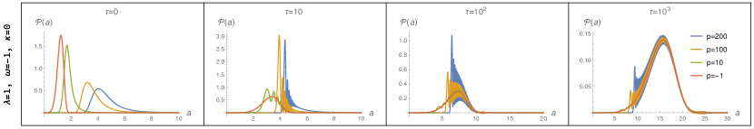
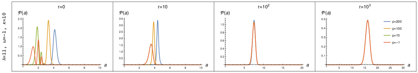
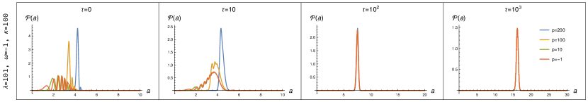
Figure 1: Time evolution of the probability distribution defined as $\mathcal{P}(a,\tau)=|\psi(a,\tau)|^{2}a^{1-3\omega-p-2q}$ associated with the wave packet in Eq. (17) for different ordering parameters and the energy distribution of fixed mean energy and varying width in the case of a cosmological constant driven universe. Profiles of different colors represent different ordering choices. The parameter associated with the width of the distribution increases across the rows as the width decreases from top to bottom, and the time increases from left to right.

The behavior of the probability distribution associated with the wave packet, i.e., $\mathcal{P}(a,\tau)=|\psi|^{2}a^{1-3\omega-p-2q}$ is shown in Fig. 1. Here, we have discussed the case of a cosmological constant driven universe, but the features observed here are generic in nature, and they appear for the other equation of state parameters as well, shown for the case of a matter dominated universe in Appendix A. We have plotted the probability distribution as a function of scale factor for different ordering choices, at different stages of the evolution and for distribution of fixed mean energy but different widths.

In the first row, we have the parameter choice that corresponds to an energy distribution of a large width. At the bounce point $\tau=0$, the probability distribution for different orderings has distinct profiles that peak at different values of the scale factor, hinting at the high sensitivity of the size of the universe at the bounce on the ordering choice. The profile corresponding to $p=-1$ peaks at the minimum value of the scale factor, and the bounce size increases as $|1+p|$ increases. As the universe expands, the probability distribution disperses in general, and profiles corresponding to large ordering parameters acquire an oscillatory character with chirp-like features, and they tend to envelop the profile for the lowest value of $p=-1$ (the probability distribution is a function of $|1+p|$). Far away from bounce, different ordering profiles completely envelop the profile for $p=-1$, and the probability distribution now peaks at the same scale factor value. For the parameter values under consideration, it seems that the oscillatory nature of the probability distribution is the distinguishing characteristic that separates the small $p$ case from the large $p$, and a large ordering parameter leads to a higher frequency and higher amplitude of the oscillations.

However, the situation reverses as we increase $\kappa$. The profiles at the bounce start to attain oscillatory features, whereas the late-time profiles start to lose the oscillatory features. The profiles for different ordering are distinct again at the bounce point, and at a later time, they merge onto the same profile, leading to the understanding that the ordering ambiguity has no imprint at a late time, in this case. As we continue to increase the parameter $\kappa$, i.e., for sharper energy distribution, the oscillatory features at the bounce keep on enhancing, and the oscillatory behavior persists away from the bounce as well.

From the analysis of the probability distribution, it is apparent that the ordering effects are most pronounced at the bounce point, where the probability distribution for different ordering parameters has different characteristics. During the later stages of the expansion, the imprints of ordering are apparent only for a broadly peaked energy distribution, manifested by the oscillatory nature of the probability distribution profiles, which persists away from the singularity. It is interesting to see whether the oscillatory behavior of the probability distribution at the late time can be captured by the expectation value of any observable. The behavior of probability distribution for varying mean energy and $-1<\kappa<0$ is discussed in Appendix A.

The evolution of the wave packet for a sharply peaked energy distribution and a small ordering parameter $(\kappa=100,\;p=-1)$ resembles the case of a Gaussian state for a free particle that is reflected from a hard boundary Andrews (1998); Robinett (2004). Initially, in the collapsing phase, i.e. $\tau\ll 0$, the probability distribution is a single-peaked profile. As the state evolves toward the bounce point, it starts attaining oscillatory features and is highly oscillatory at the bounce point. These oscillatory features disappear, giving a single peaked profile as the system evolves away from the bounce point. These oscillatory characteristics are conventionally attributed to the interference of the incoming part of the wave packet with the outgoing part Andrews (1998). The same interpretation holds for the wave packet under consideration, giving us the familiar notion of quantum bounce Alexandre and Magueijo (2022, 2023); Gielen and Magueijo (2023), making a good case for the small value of the ordering parameter as the preferred choice. On the other hand, the behavior of the wave packet for a broadly peaked energy distribution is highly counterintuitive, and the origin and interpretation of the oscillatory features at late times are a mystery at this juncture.

4 Imprints of Hamiltonian ordering on the quantum dynamics

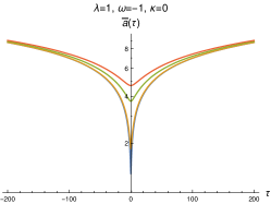
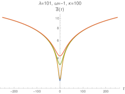
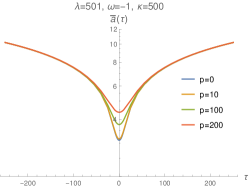
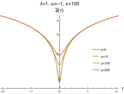
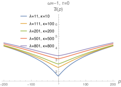
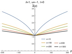
Figure 2: In the first row, the evolution of the expectation value of the scale factor for the cosmological constant driven universe with different widths of the energy distribution but fixed mean energy. Curves of different colors represent different orderings of the Hamiltonian constraint. In the first frame of the second row, we have the case for a different mean energy but the same width as for the middle frame of the first row. In the last two frames of the second row, we plot the expectation value of the scale factor at the bounce point as a function of the ordering parameter for different values of the shape parameter represented by the curves of different colors. In the middle frame of the second row, we have kept the mean energy fixed, and the width of the energy distribution decreases as $\lambda$ and $\kappa$ increase. In the last frame, we have fixed the parameter $\lambda$, so the mean energy also changes as we change $\kappa$.

We are interested in the ordering dependence of the quantum dynamics of the universe, defined by the expectation value of the scale factor. Due to the complicated nature of the wave packet, we resort to numerical computation of the expectation value using Mathematica. As alluded to in the discussion on the probability distribution, we are interested in the ordering dependence of the expectation values for two cases: a broadly peaked energy distribution, i.e., small $\kappa$, and a sharply peaked energy distribution for large $\kappa$. We consider the case of a cosmological constant driven universe, with the understanding that the generic features are present for other fluid choices as well, where the matter dominated case is shown in Appendix B.

In Fig. 2, we have plotted the expectation value of the scale factor, and it follows the trend as anticipated from the discussion about the probability distribution. The system tunnels from a collapsing branch to an expanding branch and undergoes a symmetric quantum bounce. The signature of ordering ambiguity is most pronounced at the bounce point, where scale factor expectation has a non-zero minimum and profiles for different ordering merge together for large $|\tau|$. Furthermore, we see that the expectation value of the scale factor is insensitive to the oscillatory nature of the probability distribution for the widely peaked energy distribution and follows the classical behavior for large $\tau$ regardless of the ordering or width of the energy distribution. As we decrease the width of the energy distribution, keeping its mean energy fixed, we see that the profiles of different orderings begin to merge, and one can expect a single profile for all ordering choices in the limit $\kappa\rightarrow\infty$. The time window for which the ordering effects are relevant shrinks as we increase the mean energy by increasing the parameter $\kappa$ but fixing the parameter $\lambda$, as we see in the first frame of the second row of Fig. 2. For a subclass of wave packets considered in Sahota and Lochan (2023), we analytically showed that the time scale for which the quantum effects are relevant is, in fact, related to the mean energy.

However, from the discussion thus far, it is not clear whether the ordering imprints completely disappear from the dynamics of the universe for a sharply peaked energy distribution. The signatures of ordering ambiguity are most pronounced at the bounce point, and therefore, it is prudent that we investigate the sensitivity of the expectation value of the scale factor at the bounce on the ordering of the Hamiltonian. We plot the expectation value of the scale factor at the bounce as a function of the ordering parameter for different values of the shape parameters for the fixed energy in the middle frame of the second row in Fig. 2, while the mean energy also changes in the last frame according to (16) as we keep $\lambda$ fixed.

In both cases, the bounce size is minimum for $p=-1$ and is a monotonically increasing function of $|p+1|$. As we increase the sharpness of the energy distribution, this minimum bounce size continues to increase, and the slope of dependence on the ordering decreases. We can anticipate that the dependence on the ordering will be minimal in the limit of $\kappa\rightarrow\infty$. However, it is not apparent from the middle frame of the second row in Fig. 2 that the ordering imprints indeed wash away for the fixed mean energy. On the other hand, for fixed $\lambda$, as we continue to increase $\kappa$, $\bar{a}_{0}(p)$ curve continues to flatten, and we can anticipate a flat curve parallel to the p-axis for a sharply peaked state in this case. Surprisingly, the minimum value of the bounce size for the parameter $p=-1$ remains the same for different values of the shape parameters and for fixed $\lambda$. All other ordering choices approach this value in the limiting case of $\kappa\rightarrow\infty$. Since the mean energy changes as we change $\kappa$, for a sharply peaked distribution with a large mean energy, the ordering imprints are minimal.

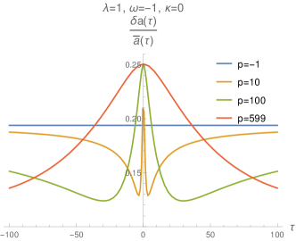
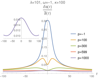
Figure 3: Relative standard deviation in scale factor as a function of time for different ordering choices, for a cosmological constant driven universe. In the first frame, we have the case of a broadly peaked distribution, and a sharply peaked distribution in the second frame.

Next, we are interested in the dynamics of fluctuations in the scale factor for different ordering choices. We plot the relative standard deviation in the scale factor as a function of time for the broadly peaked energy distribution in the first frame of Fig. 3 and the sharply peaked distribution in the second frame. The relative standard deviation turns out to be independent of time for the parameter choice $\kappa=|1+p|/3(1-\omega)$, and for other ordering choices, the relative standard deviation asymptote to this value far away from the bounce. The generic behavior of quantum fluctuations for a broadly peaked distribution is that it has a global maximum at the bounce that is sandwiched between two global minima, and it asymptotically reaches the limiting value at late time. For a larger ordering parameter, the location of global minima is pushed away from the bounce, although the magnitude of global maximum does not change. A point of reflection, in this case, is that the signatures of ordering ambiguity persist far away from the bounce, where the quantum fluctuations are not decaying but are increasing toward the limiting value asymptotically. Another observation is that the magnitude of the quantum fluctuations near the bounce is of the same order as compared to the late-time quantum fluctuations for all ordering choices.

The quantum fluctuations for sharply peaked states show a further intriguing character. For the shape parameter $\kappa=100$, the limiting case of constant quantum fluctuation is for the ordering choice $p=599$. The other ordering choices again asymptote to this value far away from the bounce. The nature of the extremum of quantum fluctuations at the bounce depends on the ordering choice. For the ordering parameter $p=-1$, the quantum fluctuations have a maximum at the bounce and monotonically decrease for large $|\tau$. For $|1+p|<599$, the quantum fluctuations have a local minimum at the bounce sandwiched between two global maxima, where the magnitude of global minima is decreasing as $|1+p|$ increases, reaching the limiting value for $p\sim 300$. For the limiting case $p=599$, the relative quantum fluctuations are constant, and as $p$ increases further, the quantum fluctuations at bounce attain a global maximum that is sandwiched between the global minima, as shown in the inset of the second frame in Fig. 3. In this case, the asymptotic behavior of the quantum fluctuation far away from the bounce is a distinguishing feature, where it decreases towards the limiting value for $|1+p|<599$, and it increases towards the limiting value for $|1+p|>599$. Furthermore, for certain ordering choices, i.e., small $p$, quantum fluctuations near the bounce are substantially larger than late-time quantum fluctuations. On the other hand, for large $p$ the magnitude of quantum fluctuations near the bounce is of the same order as compared to late-time quantum fluctuations. In general, the magnitude of late-time quantum fluctuations decreases as we decrease the width of the energy distribution.

At this point, a comment on the ordering scheme used in the literature is in order. The energy distribution considered in this work is used in numerous related works Alvarenga and Lemos (1998); Alvarenga et al. (2002); Batista et al. (2002); Hájíček and Kiefer (2001); Pedram et al. (2007a, b); Pedram and Jalalzadeh (2008); Pedram et al. (2008). To obtain analytical results, one needs to make a choice about the distribution parameter and the ordering parameter similar to the one followed in Kiefer and Schmitz (2019); Sahota and Lochan (2021, 2023), where the order of the Bessel function in Eq. (10) is chosen to be equal to the parameter $\kappa$. The issue is that once we choose an ordering scheme that generically corresponds to small $p$, the width of the distribution is large by default. Therefore, the ordering ambiguity will be relevant in addition to large quantum fluctuations, and the notion of the quantum-corrected spacetime is, therefore, ill-defined in these analyses.

In conclusion, near-bounce quantum dynamics is highly sensitive to the ordering chosen, and its imprint is most pronounced for states constructed from a broadly peaked energy distribution. The signature of operator ordering ambiguity is minimal, and the quantum fluctuations are small for states sharply peaked on a quantum-corrected trajectory. These states are of particular importance, as they are at the center of the dressed-metric approach in Ashtekar et al. (2009), and the notion of the quantum-corrected spacetime is well-defined for these states Sahota and Lochan (2023). Thus, we have shown that the ordering effects left a minimal imprint in the case of the class of states relevant to the semiclassical analysis. On the other hand, we expect the ordering to be irrelevant for a Dirac delta-like state, i.e., with $\Delta E=0$ or the stationary state in (10). However, these states are not part of the Hilbert space but the space of distributions, i.e., the antidual space in the Gelfand triplet de la Madrid (2005), in the same spirit as plane waves. The realistic scenario is that we have a state with finite although small $\Delta E/\bar{E}$, and therefore, the system will always have some sensitivity to the ordering chosen.

5 Discussion

We have investigated imprints of ordering ambiguity on the dynamics of a perfect fluid dominated quantum universe. A general ordering scheme is employed for the Hamiltonian operator and a wave packet is constructed that represents the quantum bounce. We start with the analysis of the probability distribution associated with the wave packet. The wave packet with sharply peaked energy distribution and small ordering parameter has a direct correspondence with a Gaussian state reflecting from a hard wall; in other cases, the behavior of the probability distribution is highly non-trivial. In the case of wave packets with a broadly peaked energy distribution, the probability distribution has oscillatory features at late times for a large ordering parameter, providing a possible avenue to investigate the signatures of ordering ambiguity.

The expectation value of the scale factor represents a robust, symmetric bounce with appropriate classical behavior away from the singularity. The quantum dynamics of the universe turn out to be insensitive to the oscillatory character of the probability distribution at a late time in the expanding phase. As the width of the energy distribution decreases, the profiles with different orderings tend to merge, and we expect the ordering imprints to wash away in this regime. The ordering imprints are most pronounced at the bounce, and we investigate the dependence of the bounce size on the ordering parameter for different values of the shape parameter. We find that the scale factor expectation is insensitive to the ordering chosen for sharply peaked states. The analysis suggests that the ordering imprints are washed away in the limit of the energy distribution of the vanishing width and the large mean energy. Moreover, we show that the quantum fluctuations in scale factor are of the same order throughout the evolution of the universe for broadly peaked states, whereas they are decaying to small albeit finite value far away from bounce for sharply peaked states. However, the ordering choice does dictate the near-bounce behavior of quantum fluctuations even for sharply peaked states.

We show that quantum ambiguities are of little relevance and that late-time quantum fluctuations are small for a universe with a well-defined energy, i.e., $\Delta E\ll\overline{E}$. The conjecture of sharply peaked state turns out to be a savior from the quantization ambiguities in the effective geometry approach Ashtekar et al. (2009); Sahota and Lochan (2023) in the case of this toy model, and the expectation value of scale factor provides a consistent quantum-corrected spacetime. However, the ordering choice will leave some signature on the cosmological observables through their imprint on the size from which the universe bounces off and the quantum fluctuations in the scale factor for physical states (which are not infinitely peaked with $\Delta E=0$). In standard quantum cosmology analysis, the Vilenkin or Laplace-Beltrami ordering choice leads to large quantum fluctuations and leaves an imprint of ordering ambiguity for states considered in Alvarenga and Lemos (1998); Alvarenga et al. (2002); Batista et al. (2002); Pedram et al. (2007a, b); Pedram and Jalalzadeh (2008); Pedram et al. (2008). On a side note, one wonders whether the conjecture of sharply peaked states can save other canonical approaches to quantum gravity, e.g., the dressed metric approach Ashtekar et al. (2009); Agullo et al. (2013a, 2012), from the operator ordering ambiguities as well.

6 Acknowledgments

HSS acknowledges the financial support from the University Grants Commission, Government of India, in the form of Junior Research Fellowship (UGC-CSIR JRF/Dec-2016 /503905). HSS thanks Kinjalk Lochan and Vikramaditya Mondal for the careful reading of manuscript, and for their comments and suggestions. HSS is grateful to Patrick Peter and Przemyslaw Malkiewicz for the helpful discussions during the early stage of this work and their hospitality during his visit to IAP Paris and NCBJ Warsaw. HSS is grateful to the organizers of the conference ‘Time and Clocks’ for the hospitality at Physikzentrum Bad Honnef and thanks Martin Bojowald for his comments on my previous work that initiated this project.

Appendix A Evolution of wave packet

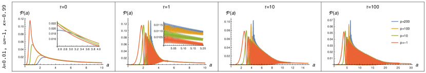
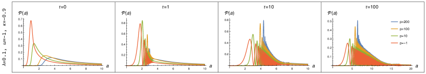
Figure 4: Time evolution of the probability distribution associated with the wave packet in Eq. (17) for different ordering parameters and the energy distribution of fixed mean energy and broadly peaked width in the case of a cosmological constant driven universe. Profiles of different colors represent different ordering choices.

In this appendix, we discuss the evolution of wave packet for the cases not considered in the main text. In Fig. 4, we have plotted the probability distribution for the case where $-1<\kappa<0$, where the width of the energy distribution is comparatively larger. In this case, we see that the behavior of probability distribution is even more peculiar with no apparent correspondence between different ordering choices at any stage of the evolution of the universe.

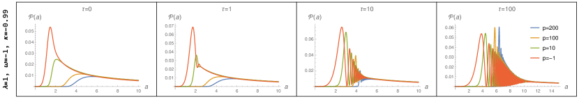
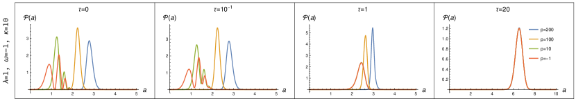
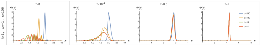
Figure 5: Time evolution of the probability distribution for different ordering parameters and the energy distribution of varying mean energy and varying width in the case of a cosmological constant driven universe.

In Fig. 5, we change the mean energy of the distribution as well as its width. We see that the dynamics of the probability distribution have the same generic features as we have seen for the previous case, although notably, the ordering imprints for a sharply peaked state sustain for a shorter duration only. Again, we have late-time oscillatory features in the probability distribution for the broadly peaked energy distribution, and for the sharply peaked energy distribution, we have oscillatory features at the bounce. Therefore, it seems that the behavior of the probability distribution is sensitive to the sharpness of the energy distribution rather than to the mean energy. In Fig. 6, we show that the characteristic features in the dynamics of the probability distribution are present for a matter dominated universe as well.

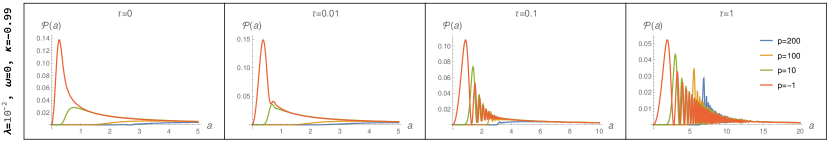
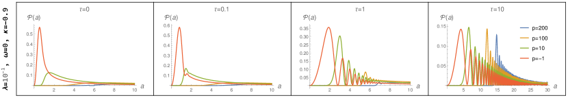
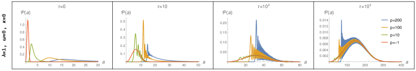
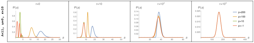
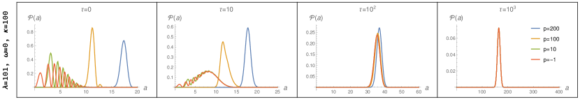
Figure 6: Time evolution of the probability distribution for different ordering parameters and the energy distribution of fixed energy and of varying width in case of a matter dominated universe.

Appendix B Evolution of the dust dominated quantum universe

In this appendix, we discuss the quantum evolution of a dust dominated universe. In the first row of Fig. 7, we have plotted the expectation value of the scale factor for different ordering choices and for the energy distribution of fixed mean energy and decreasing width. We see the results follow the cosmological constant driven universe considered in the main text, the ordering imprints are most pronounced at the bounce, the domain of ordering dependence is shrinking, and the different ordering profiles tend to merge with decreasing width. Moreover, as we increase the mean energy, the time window of ordering dependence decreases by several orders of magnitude. In the second row of Fig. 7, we plot the quantum fluctuations in the scale factor in the last two frames. In this case, the numerical computation for broadly peaked state and far away from bounce is stable, and we see that the fluctuations for different ordering choices tend to limiting case. For quantum fluctuations as well, the dust-dominated universe has the same characteristic features as in the case of the cosmological constant driven universe.

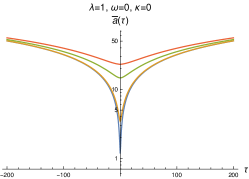
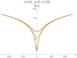
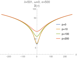
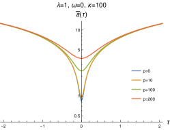
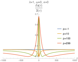
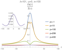
Figure 7: The expectation value of the scale factor for the cosmological constant driven universe in the first row and the dust dominated universe in the second row with different values of the shape parameter $\kappa=0$, $\kappa=100$ and $\kappa=500$, but fixed mean energy. Curves with different colors represent different orderings of the Hamiltonian constraint. In the third row, we have the case for different mean energy.

References

- Kiefer (2012) C. Kiefer, Quantum gravity, third edition ed., International series of monographs on physics No. 155 (Oxford University Press, Oxford, 2012).
- DeWitt (1967) B. S. DeWitt, Quantum Theory of Gravity. I. The Canonical Theory, Physical Review 160, 1113 (1967).
- Tsamis and Woodard (1987) N. C. Tsamis and R. P. Woodard, The factor-ordering problem must be regulated, Phys. Rev. D 36, 3641 (1987).
- Halliwell (1988) J. J. Halliwell, Derivation of the wheeler-dewitt equation from a path integral for minisuperspace models, Phys. Rev. D 38, 2468 (1988).
- Hawking and Page (1986) S. W. Hawking and D. N. Page, Operator Ordering and the Flatness of the Universe, Nucl. Phys. B 264, 185 (1986).
- Vilenkin (1988b) A. Vilenkin, Quantum cosmology and the initial state of the universe, Phys. Rev. D 37, 888 (1988b).
- Louko (1988) J. Louko, Semiclassical Path Measure and Factor Ordering in Quantum Cosmology, Annals Phys. 181, 318 (1988).
- (8) J. J. Halliwell, “Derivation of the wheeler-dewitt equation from a path integral for minisuperspace models,” Phys. Rev. D 38 (Oct, 1988) 2468–2481.
- Bojowald (2002) M. Bojowald, Isotropic loop quantum cosmology, Class. Quant. Grav. 19, 2717 (2002), arXiv:gr-qc/0202077 .
- (10) N. Kontoleon and D. L. Wiltshire, “Operator ordering and consistency of the wave function of the universe,” Phys. Rev. D 59 (1999) 063513, arXiv:gr-qc/9807075.
- Bojowald and Simpson (2014) M. Bojowald and D. Simpson, Factor ordering and large-volume dynamics in quantum cosmology, Class. Quant. Grav. 31, 185016 (2014), arXiv:1403.6746 [gr-qc] .
- Rostami et al. (2015) T. Rostami, S. Jalalzadeh, and P. V. Moniz, Quantum cosmological intertwining: Factor ordering and boundary conditions from hidden symmetries, Phys. Rev. D 92, 023526 (2015).
- Kiefer and Schmitz (2019) C. Kiefer and T. Schmitz, Singularity avoidance for collapsing quantum dust in the Lemaître-Tolman-Bondi model, Physical Review D 99, 126010 (2019)..
- (14) H. Matsui, S. Mukohyama, and A. Naruko, “DeWitt boundary condition is consistent in Hořava-Lifshitz quantum gravity,” Phys. Lett. B 833 (2022) 137340, arXiv:2111.00665 [gr-qc].
- Sahota and Lochan (2021) H. S. Sahota and K. Lochan, Infrared signatures of a quantum bounce in a minisuperspace analysis of lemaître-tolman-bondi dust collapse, Phys. Rev. D 104, 126027 (2021).
- Sahota and Lochan (2023) H. S. Sahota and K. Lochan, “Analyzing quantum gravity spillover in the semiclassical regime,” The European Physical Journal C 83, 1162 (2023), arXiv:2211.16426 [gr-qc] .
- Thebault (2023) K. P. Y. Thebault, Big bang singularity resolution in quantum cosmology, Class. Quant. Grav. 40, 055007 (2023), arXiv:2209.05905 [gr-qc] .
- Bojowald (2007) M. Bojowald, Dynamical coherent states and physical solutions of quantum cosmological bounces, Phys. Rev. D 75, 123512 (2007).
- Ashtekar et al. (2009) A. Ashtekar, W. Kaminski, and J. Lewandowski, Quantum field theory on a cosmological, quantum space-time, Phys. Rev. D 79, 064030 (2009), arXiv:0901.0933 [gr-qc] .
- Agullo et al. (2013a) I. Agullo, A. Ashtekar, and W. Nelson, Extension of the quantum theory of cosmological perturbations to the Planck era, Phys. Rev. D 87, 043507 (2013a), arXiv:1211.1354 [gr-qc] .
- Agullo et al. (2012) I. Agullo, A. Ashtekar, and W. Nelson, A Quantum Gravity Extension of the Inflationary Scenario, Phys. Rev. Lett. 109, 251301 (2012), arXiv:1209.1609 [gr-qc] .
- Agullo et al. (2013b) I. Agullo, A. Ashtekar, and W. Nelson, The pre-inflationary dynamics of loop quantum cosmology: Confronting quantum gravity with observations, Class. Quant. Grav. 30, 085014 (2013b), arXiv:1302.0254 [gr-qc] .
- Kiefer (1994) C. Kiefer, The Semiclassical approximation to quantum gravity, Lect. Notes Phys. 434, 170 (1994), arXiv:gr-qc/9312015 .
- Schutz (1970) B. F. Schutz, Perfect fluids in general relativity: Velocity potentials and a variational principle, Phys. Rev. D 2, 2762 (1970).
- Schutz (1971) B. F. Schutz, Hamiltonian theory of a relativistic perfect fluid, Phys. Rev. D 4, 3559 (1971).
- (26) G. Arfken and H. Weber, Mathematical Methods for Physicists, 6th ed. (Academic Press, Boston, 2005).
- Hájíček and Kiefer (2001) P. Hájíček and C. Kiefer, Singularity avoidance by collapsing shells in quantum gravity, International Journal of Modern Physics D 10, 775 (2001).
- BALLENTINE (1970) L. E. Ballentine, The Statistical Interpretation of Quantum Mechanics, Rev. Mod. Phys. 42, 358 (1970).
- GRADSHTEYN and RYZHIK (1980) I. Gradshteyn and I. Ryzhik, 6.-7 - definite integrals of special functions, in Table of Integrals, Series, and Products, edited by I. Gradshteyn and I. Ryzhik (Academic Press, 1980) pp. 635–903.
- Andrews (1998) M. Andrews, Wave packets bouncing off walls, American Journal of Physics 66, 252 (1998), https://pubs.aip.org/aapt/ajp/article-pdf/66/3/252/11525613/252_2_online.pdf .
- Robinett (2004) R. Robinett, Quantum wave packet revivals, Physics Reports 392, 1 (2004).
- Alexandre and Magueijo (2022) B. Alexandre and J. Magueijo, Possible quantum effects at the transition from cosmological deceleration to acceleration, Phys. Rev. D 106, 063520 (2022), arXiv:2207.03854 [gr-qc] .
- Alexandre and Magueijo (2023) B. Alexandre and J. Magueijo, Unimodular Hartle-Hawking wave packets and their probability interpretation, Phys. Rev. D 107, 063501 (2023), arXiv:2210.02179 [hep-th] .
- Gielen and Magueijo (2023) S. Gielen and J. Magueijo, Quantum analysis of the recent cosmological bounce in the comoving Hubble length, Phys. Rev. D 107, 023518 (2023), arXiv:2201.03596 [gr-qc] .
- Alvarenga and Lemos (1998) F. G. Alvarenga and N. A. Lemos, Dynamical vacuum in quantum cosmology, Gen. Rel. Grav. 30, 681 (1998), arXiv:gr-qc/9802029 .
- Alvarenga et al. (2002) F. G. Alvarenga, J. C. Fabris, N. A. Lemos, and G. A. Monerat, Quantum cosmological perfect fluid models, Gen. Rel. Grav. 34, 651 (2002), arXiv:gr-qc/0106051 .
- Batista et al. (2002) A. B. Batista, J. C. Fabris, S. V. B. Goncalves, and J. Tossa, Quantum cosmological perfect fluid model and its classical analog, Phys. Rev. D 65, 063519 (2002), arXiv:gr-qc/0108053 .
- Pedram et al. (2007a) P. Pedram, S. Jalalzadeh, and S. S. Gousheh, Schrodinger-Wheeler-DeWitt equation in chaplygin gas FRW cosmological model, Int. J. Theor. Phys. 46, 3201 (2007a), arXiv:0705.3587 [gr-qc] .
- Pedram et al. (2007b) P. Pedram, S. Jalalzadeh, and S. S. Gousheh, Quantum Stephani exact cosmological solutions and the selection of time variable, Class. Quant. Grav. 24, 5515 (2007b), arXiv:0709.1620 [gr-qc] .
- Pedram and Jalalzadeh (2008) P. Pedram and S. Jalalzadeh, Quantum FRW cosmological solutions in the presence of Chaplygin gas and perfect fluid, Phys. Lett. B 659, 6 (2008), arXiv:0711.1996 [gr-qc] .
- Pedram et al. (2008) P. Pedram, M. Mirzaei, S. Jalalzadeh, and S. S. Gousheh, Perfect fluid quantum Universe in the presence of negative cosmological constant, Gen. Rel. Grav. 40, 1663 (2008), arXiv:0711.3833 [gr-qc] .
- de la Madrid (2005) R. de la Madrid, “The role of the rigged hilbert space in quantum mechanics,” European Journal of Physics 26, 287–312 (2005).