Solving Max-Min Fair Resource Allocations Quickly on Large Graphs

Abstract– We consider the max-min fair resource allocation problem. The best-known solutions use either a sequence of optimizations or waterfilling, which only applies to a narrow set of cases. These solutions have become a practical bottleneck in WAN traffic engineering and cluster scheduling, especially at larger problem sizes. We improve both approaches: (1) we show how to convert the optimization sequence into a single fast optimization, and (2) we generalize waterfilling to the multi-path case. We empirically show our new algorithms Pareto-dominate prior techniques: they produce faster, fairer, and more efficient allocations. Some of our allocators also have theoretical guarantees: they trade off a bounded amount of unfairness for faster allocation. We have deployed our allocators in Azure’s WAN traffic engineering pipeline, where we preserve solution quality and achieve a roughly $3\times$ speedup.

1 Introduction

Multi-resource fair allocators have become essential for cloud operators as multi-tenancy, availability, and efficiency grow in importance. These allocators divide the resources fairly among different requests (applications, users, or network flows). Operators use them to meet customer expectations, especially during congestion and for network neutrality.

Recent works present fair allocators in settings such as WAN traffic engineering [17, 30, 34, 38] and GPU scheduling [14, 42, 56]. We show these allocators achieve fairness at the cost of speed (crucial for maintaining high utilization as loads change [4]) and efficiency (essential for profit).

We aim to achieve a better balance between fairness, efficiency, and speed, and our novel algorithms offer operators greater flexibility to control the trade-off between them. We focus on max-min fairness — where we cannot allocate more to one request without reducing the allocation of another with an equal or smaller value — because it is simple, commonly used in practice [30, 34, 39, 56], and can promote efficiency.

Figure 1: Comparing the new allocators with state-of-the-art. Soroush offers parameterizable max-min fair allocators. The axes are fairness and speed; the marker size corresponds to efficiency (larger is more efficient). Our new allocators empirically Pareto-dominate other schemes, and some of them have theoretical guarantees on fairness (§4).

The definition of max-min fairness naturally leads to iterative solutions that prioritize smaller requests over larger ones and assign rates in order from smallest to largest. In multi-resource settings, these solutions solve either mixed-integer or linear optimizations [52, 59] at each step. Their scalability depends on the size of each individual optimization and the number of iterations – typically a function of the number of resources and requests.

Operators need to invoke resource allocators when workloads change or failures occur. However, today’s exact [17, 56] or approximate solutions (e.g., that trade-off fairness for speed [30]) are too slow in reacting to these events at the production scale. They take tens of minutes to hours (§4) on WANs with 100s of routers that serve millions of flows or clusters with 1000s of jobs.

We ask: are iterative optimizations necessary for max-min fair resource allocation? Max-min fair algorithms must maximize smaller allocations before assigning more capacity to larger ones. Current solutions iterate because they do not know the sorted order of these rate allocations apriori. One of our ideas is to (1) use sorting networks [7] to discover the sorted order of max-min fair allocations dynamically within the optimization and (2) use a linear weighted objective that explicitly incentivizes the optimization to allocate more rates to requests with smaller indices in the sorted order. The result is a single-shot optimization for max-min fair allocation.

The above single-shot optimization is not always practical as modeling sorting networks within an optimization can significantly increase its size, and the linear weighted objective can cause double-precision issues when there are many requests. To develop a practical solution, we combine this idea with an approximate max-min fair allocator from SWAN [30]. This combination results in a new allocator, GeometricBinner (or GB), which is fundamentally faster than SWAN, does not need sorting networks, has no double precision issues, and provides the same fairness guarantees as SWAN.

Waterfilling-based algorithms [8] can be faster than black-box optimizations, but they are specialized for cases where each request seeks rates on a single path. In a broad class of problems [14, 17, 30, 34, 38, 42, 56], requests ask for allocation from multiple paths. In these cases, the global fair share is not locally fair along each path, and waterfilling does not apply. Our solution, AdaptiveWaterfiller (or AW), extends waterfilling to multi-path settings. AW is faster than GB but does not have a worst-case fairness guarantee. We prove AW can converge to a small set of allocations that contain the optimal.

Our third algorithm, which is empirically the fairest, combines the above approaches. We apply GB with one change: use the allocations from AW to spread requests more uniformly among bins (instead of the fixed geometrically increasing bin sizes in GB). This allocator, EquidepthBinner (or EB), is slower than both AW and GB (executes each once) but intuitively improves fairness for the same reason that equi-depth binning reduces histogram approximation error [32].

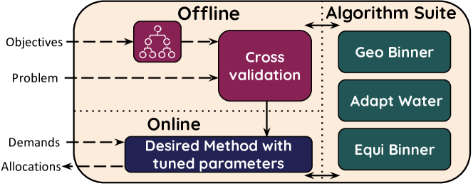
Soroush is the collection of these algorithms, each providing a different trade-off among fairness, efficiency, and speed. Operators can use our simple decision process to choose the allocator (and its hyper-parameters) that achieves their desired trade-off. Table 1 lists our allocators, their theoretical and empirical properties, and their parameters.

Allocator	Properties	Parameters
Geometric	(T) $\alpha$-approx fairness guarantee	$\alpha$
Binner	(E) Faster than other $\alpha$-approx methods	$\epsilon$
Adaptive	(T) Solution in a small set containing optimal	#iterations
Waterfiller	(E) Fastest
Equi-depth	(T) Better than Adaptive Waterfiller	#iterations
Binner	(E) Fairest and fast	#bins, $\epsilon$

Table 1: The Soroush allocators, their properties (Theoretical and Empirical), and their parameters. These allocators provide different trade-offs among fairness, efficiency, and speed.

To show Soroush is general, we introduce a graph model for multi-resource, max-min fair resource allocation problems where edges model resources and paths capture groups of resources the allocator must assign together. Requests (demands) can then ask for resources on any choice of multiple paths. This compact and general model subsumes problems from at least two domains: traffic engineering (TE) and cluster scheduling (CS). Soroush can solve any future max-min fair allocation problem if the user can specify it in this model.

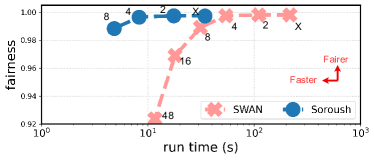
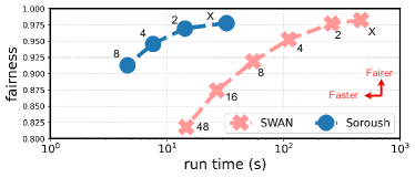
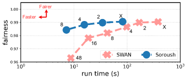
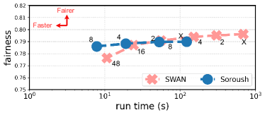
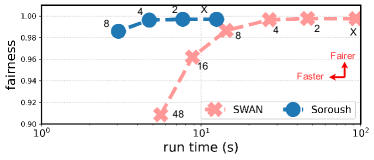
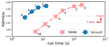
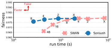
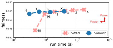
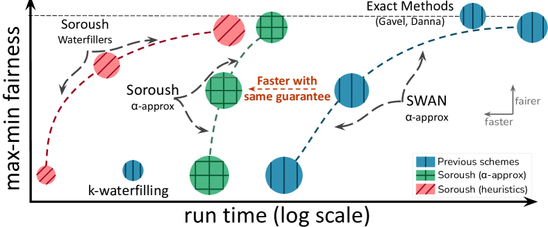
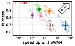
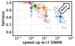
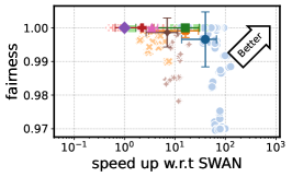
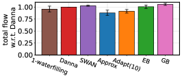
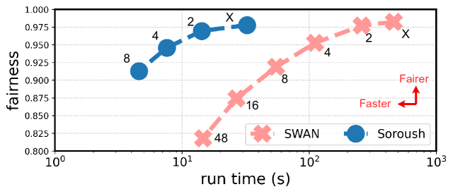
Our extensive evaluation in both TE and CS (which we summarize in Fig. 1) show the new allocators Pareto-dominate the state-of-the-art in fairness, speed, and efficiency.

We deployed GeometricBinner in the production TE pipeline at Azure where it provides a $2.4\times$ average speedup (up to $5.4\times$ in some cases) without any impact on fairness and efficiency compared to the previous allocator.

2 Motivation and Overall Approach

Figure 2: Slow max-min fair resource allocators cause under-utilization and unfairness. We compare two instances of the SWAN solver – one computes the allocations instantly while the other needs two windows – on a $5$-hour trace from Azure’s WAN. The results indicate a large gap between the two solutions in fairness and efficiency.

Faster workload dynamics [4] and higher availability requirements [45] have made fast resource allocation a necessity. Operators of multi-tenant clouds further require solutions that ensure fairness and maintain high efficiency [30, 34]. Prior work ([4, 45, 55, 66] in TE or [56] in CS) fails to meet one or more of these requirements.

Efficient and fair solvers [17, 30, 56] cannot adapt quickly to conditions that frequently change. Some production environments [4] use the most recent previous allocation when the solver cannot allocate resources within a fixed time window. This is sub-optimal: nodes that increase their demands in the new window do not get enough resources, and others who request less may receive more than they need.

Figure 3: State-of-the-art methods can not keep up with frequently changing demands. We capture the number of windows (left) and the number of iterations (right) each approach needs. To keep up with demands, they must finish within a single 5-minute window. However, SWAN [30] and Danna et al. [17] often need more than one window and miss their deadline. The results are on a topology with $\sim$200 nodes and $\sim$500 edges. Left captures 160 different scenarios. Right is a highly loaded scenario [4] – the results hold across all the algorithms in Soroush.

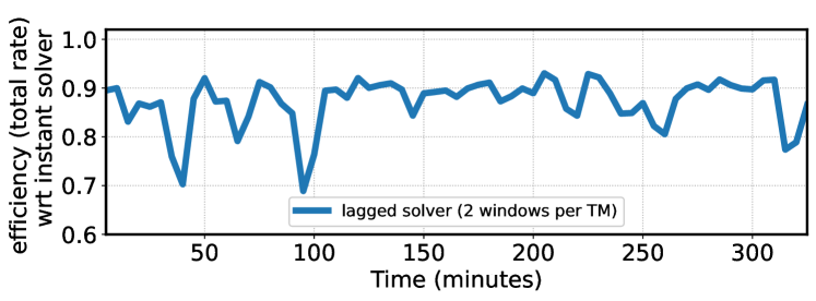
We quantify the impact of this strategy in the TE setting using a $5$-hour trace from Azure’s production WAN (Fig. 2), which uses a $5$-minute window. We observe a solver that needs two windows ($10$ minutes) to allocate resources reduces fairness by $20$% – $60$% and efficiency by $10$% – $30$% relative to a solver that completes within one window.

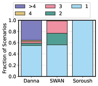
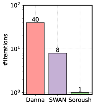
How often do solvers miss their deadline? We use traces from [4] to show the distribution of the number of windows an exact solver (Danna et al. [17]) and Microsoft’s approximate solver (SWAN [30]) need to compute max-min fair allocations. For nearly half of the traffic trace, these solvers exceed the $5$-minute window and often need $2$ to $3$ windows to finish (Fig. 3, left). This is because these approaches invoke expensive optimizations multiple times (Fig. 3, right).

Soroush invokes at most one optimization and always completes within a single window. Whether a one-shot optimization is faster than an iterative approach that solves multiple optimizations depends on two factors: (a) the number of optimizations in the iterative approach, and (b) the size of the optimization in the one-shot approach compared to those in the iterative solution. Our one-shot optimizations are faster than previous solutions [17, 30, 56] because we only add a small number of variables to convert the problem into one that can be solved in one shot, and we avoid the overhead in solving multiple optimizations. See §F for a detailed analysis.

While examples here are from TE, CS resource allocators are similar [56]. We omit the details for brevity.

2.1 Our model

We model the max-min fair resource allocation problem as a capacitated graph. Each edge represents a different resource, and edge capacities show the amount of available resources. Paths in the graph encode a collection of resources we must allocate together (e.g., GPU and memory), and demands can request resources on a subset of these paths. Our model also supports other affine constraints over graph variables (e.g., text in maroon below). Soroush solves any max-min fair resource allocation problem we can specify in this model.

Our model takes as input:

• A set of resources $\mathcal{E}$, each with capacities $c_{e},e\in\mathcal{E}$.

• A set of paths $\mathcal{P}$ where each path is a group of dependent resources that we must allocate together.

• A set of demands $\mathcal{D}$ where each demand $k\in\mathcal{D}$:

  • Requests some rate $d_{k}$.

  • Has weight $w_{k}$ (for weighted max-min fairness).

  • Can be routed over a set of multiple paths $P_{k}\in\mathcal{P}$.

  • Consumes $r_{k}^{e}$ of the capacity on edge $e$ for each unit rate we assign.

  • Has utility $q_{k}^{p}$ on path $p$ for each unit rate.

A max-min fair allocator assigns rates to demands such that the weighted ratios $\{\frac{f_{k}}{w_{k}}\}$ are max-min fair: to increase the allocation of any demand, we have to reduce the allocation of another demand with a smaller ratio.

Term	Interpretation
$\mathcal{E},\mathcal{D},\mathcal{P}$	sets of resources, demands and paths
$c_{e}$	capacity of resource $e\in\mathcal{E}$
$\mathbf{f},f_{k}^{p}$	rate allocation vector and rate for demand $k$ on path $p$
$d_{k},w_{k}$	requested rate and weight for demand $k\in\mathcal{D}$
$r^{e}_{k},q^{p}_{k}$	scaling resource consumption and rate utility for demand $k$

Table 2: Notation for our max-min fair resource allocation model. (more details in Table A.1)

Figure 4: Choosing allocators (and their parameters).

We can use this model to specify max-min fair allocation problems in traffic engineering (TE) [30, 34] and cluster scheduling (CS) [56, 22, 25].

TE. The actual links in the network are the resources, and demands are services that require a specific rate between nodes in the network. The TE scheme picks the paths for each demand. Weights describe how the operator wants to divide the rates (e.g., split rate between search and ads services).

CS. Each path corresponds to a server and contains multiple edges. Each edge models a different type of resource on each server (e.g., CPU, memory, or GPU). Demands are jobs that require a number of workers. We model heterogeneity (workers may progress at different rates on different servers) with the utility term $q_{k}^{p}$ and scale how much of each resource the worker uses with $r_{k}^{e}$. We also support extensions, such as jobs with varying resource requirements [22, 25].

We are unaware of any model as general as ours for max-min fair allocation. However, solving this general model is hard: when we must allocate resources along multiple paths (groups of resources), local fairness does not imply global fairness, so single-path solutions [36] are ineffective. In Soroush, we focus on this model and leave the extension to problems that we cannot model as graphs [21] for future work.

2.2 Soroush Overview

Soroush offers a suite of allocators that produce approximate solutions for graph-based max-min fair allocation problems. An allocator is either an algorithm or optimization (or a combination of both) that assigns max-min fair rates that meet the demand and capacity constraints.

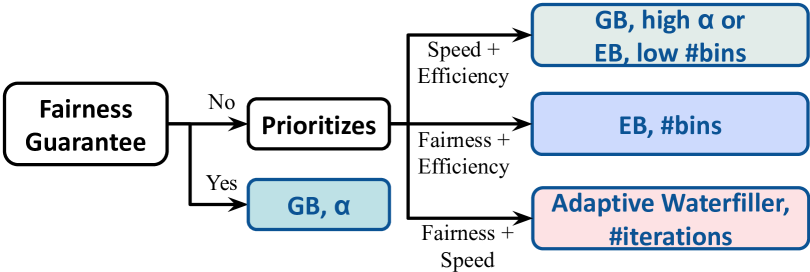
Table 1 lists our allocators, their key properties, and salient parameters that let the user trade-off between fairness, speed, and efficiency (see §3 for more details). We have many choices here and naïvely running multiple allocators in parallel can waste computational resources. We suggest a simple decision process along with a hyperparameter search to help practitioners choose a suitable allocator (Fig. 4 and 5). A sensitivity analysis in §4 indicates that this decision process is robust. We do not claim any credit for it but use it as evidence that we have effective mechanisms to make the choice.

The GeometricBinner (§3.1) is the only allocator in Soroush with worst-case fairness guarantees: for a given $\alpha>1$, it provably assigns rates to each demand within $[\alpha^{-1},\alpha]$ times its optimal max-min fair rate. EquidepthBinner (§3.3) is the best choice for users who prefer fairness and efficiency but do not need formal worst-case guarantees. AdaptiveWaterfiller (§3.2) is suitable for users who prefer speed over efficiency.

Figure 5: An example of how to pick the right allocator.

3 Max-Min Fair Resource Allocators

We present two novel kinds of multi-resource max-min fair resource allocation algorithms.

3.1 One-shot Optimizations

Overview. We can think of max-min fair resource allocation as an optimization with a prioritized list of objectives: first, we maximize the smallest allocation, then the second smallest, and so on. This intuition naturally leads to a sequence of linear optimization problems (LPs) [17, 30].

Prior exact methods are slow since they solve nearly as many LPs as the number of unique resources [17] (number of edges in a network or machines in a cluster).

We will show how to linearize a prioritized list of objectives such that we can solve one optimization instead of a (long) sequence. The optimization we arrive at is analytically interesting but can encounter double-precision errors, requires a sorting network to sort allocations, and is consequently slower in practice — we instead linearize an approximate version.

SWAN [30] uses an approximate solution that needs to solve fewer LPs. It gradually and geometrically increases the maximum possible rate for each demand and guarantees the final allocations are within $\alpha\times$ their optimal fair rates. Users pick an $\alpha$ based on their requirements for fairness and speed (e.g., $\alpha=2$ in SWAN). A larger $\alpha$ requires fewer LPs but results in less fair allocations. Microsoft has been using SWAN in production for many years [39].

We develop an approximate one-shot optimization by linearizing SWAN’s approximate geometric method. Our idea is to define “bins” that capture the geometric rate increase at each iteration and introduce new variables to model each flow’s allocation from each bin instead of the cumulative total. This combination of techniques is novel and has the same worst-case fairness guarantees as SWAN. By linearizing at the granularity of bins, we no longer encounter double precision issues, do not need a sorting network, and achieve an empirically faster solution.

We flesh out the details next (Tables 2 and 3 show our notations). We discuss why this one-shot optimization is fundamentally smaller and faster than SWAN’s sequence of optimizations. We present results from our production deployment in §4.2.

Max-min fair allocation as a sequence of LPs. If we have $n$ demands, we can use $n$ LPs to compute max-min fair allocations — the $i^{\mbox{\tiny{th}}}$ LP in the sequence maximizes the $i^{\mbox{\tiny{th}}}$ smallest rate. Let $t_{i}$ be the $i^{\mbox{\tiny{th}}}$ smallest rate, then:

$$\mbox{\sf MaxMin}_{i}(\mathcal{E},\mathcal{D},\mathcal{P})\leavevmode\nobreak\ \triangleq \arg\max\leavevmode\nobreak\ \leavevmode\nobreak\ t_{i}$$ (1)

s.t. $$(t_{1},\dots,t_{i-1})\in\mbox{\sf MaxMin}_{i-1}(\mathcal{E},\mathcal{D},\mathcal{P}),$$

$$f_{k}\geq t_{i},\quad\quad\forall k\leavevmode\nobreak\ \leavevmode\nobreak\ \mbox{whose rate is not yet frozen}$$

$$\mathbf{f}\in{\sf FeasibleAlloc}(\mathcal{E},\mathcal{D},\mathcal{P}).$$

Note that the algorithm freezes demands that can not receive more than $t_{i}$ in each iteration. These demands will not receive any allocations in later iterations.

Term	Meaning
$\mathbf{t}$, $t_{i}$	sorted rate vector and the $i^{\mbox{\tiny{th}}}$ smallest rate
$N_{\beta},\mathcal{D}_{b}$	number of bins and set of demands in bin $b$
${\ell}_{b},s_{b}$	boundary and slackness of bin $b$
$\mathbf{f}_{b}$, $f_{kb}$	bin allocation vector and rate of demand $k$ in bin $b$

Table 3: Additional notation for Soroush.

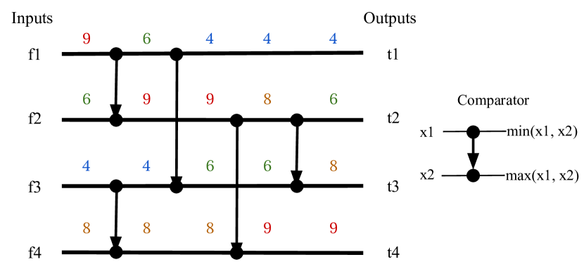
Our one-shot optimal max-min fair solution. We change Eqn. 1 (changes are in color) to a single optimization by (1) using a sorting network [7, 35, 45] to sort the rates as part of the optimization (Fig. A.1), and (2) using a linear weighted objective where the weight of a demand decreases based on its rank in the sorted order — these weights incentivize the optimization to increase the smaller rates.

Eqn. 1 does not need sorting because each LP maximizes the next smallest rate. The one-shot optimization, however, must explicitly sort the allocations in order to weight them appropriately in the objective. Let $\epsilon<1$, then:

$$\mbox{\sf OneShotOpt}(\mathcal{E},\mathcal{D},\mathcal{P})\leavevmode\nobreak\ \triangleq \arg\max_{\mathbf{f}}{\color[rgb]{0.5,0,0}\definecolor[named]{pgfstrokecolor}{rgb}{0.5,0,0}\sum_{i=1}^{n}\epsilon^{i-1}}t_{i}$$ (2)

s.t. $${\color[rgb]{0.5,0,0}\definecolor[named]{pgfstrokecolor}{rgb}{0.5,0,0}({t_{1}},\dots,{t_{n}})=\text{\sf sorted rates}(\mathbf{f}),}$$

$$\mathbf{f}\in{\sf FeasibleAlloc}(\mathcal{E},\mathcal{D},\mathcal{P}).$$

We prove OneShotOpt leads to max-min fair rates:

Theorem 1.

There exist values of $\epsilon$ for which the optimization in Eqn. 2 yields the same max-min fair rate allocations as the sequence of optimizations shown in Eqn. 1.

Proof Sketch.

Let ${\mathbf{t^{\dagger}}}$ be the rate vector solution from Eqn. 2. Notice that the optimal max-min fair rate vector, say ${\mathbf{t^{*}}}$, is a feasible solution to Eqn. 2. Thus, $\sum_{i}\epsilon^{i-1}t^{\dagger}_{i}\geq\sum_{i}\epsilon^{i-1}t^{*}_{i}$ (otherwise $\mathbf{t^{\dagger}}$ is not the optimal solution to Eqn. 2). We can re-arrange and get $t^{*}_{1}-t^{\dagger}_{1}\leq{\epsilon}\left(\sum_{i>1}\epsilon^{i-1}t^{\dagger}_{i}-\sum_{i>1}\epsilon^{i-1}t^{*}_{i}\right)$.

By definition of max-min fairness, we have $t^{*}_{1}\geq t^{\dagger}_{1}$ since $t^{*}_{1}$ is the smallest allocation in the optimal max-min fair solution. If we can find a feasible assignment where the smallest rate $t^{\dagger}_{1}$ is higher, then $t^{*}$ cannot be max-min fair — we can increase the smallest rate without hurting any other demand with an smaller allocation (because no such demand exists). These statements together imply the smallest rates must match as $\epsilon\rightarrow 0$. The rest follows by induction. ∎

OneShotOpt is not practical. We need a small $\epsilon$ to find an optimal solution (see proof), but we will encounter double precision errors if the smallest weight ($\epsilon^{n-1}$) is too small. In this case, the formulation may have to sacrifice optimality and use a large $\epsilon$ to solve the one-shot optimization (especially when there are many demands). Even with a large $\epsilon$, we find that solving LPs with a full sorting network is slow [35, 45] since sorting networks add $O(nlog^{2}(n))$ additional constraints.

Our one-shot GeometricBinner (or GB) linearizes the following approximate max-min fair technique. Compared to Eqn. 1, Eqn. 3 shows a shorter sequence of LPs inspired by SWAN [30] (changes in color) but also differs from SWAN  in one crucial way (it introduces new variables to track the increase in the allocation of each demand in each iteration):

$$\mbox{\sf ApproxMaxMin}_{{\color[rgb]{0.5,0,0}\definecolor[named]{pgfstrokecolor}{rgb}{0.5,0,0}b}}(\mathcal{E},\mathcal{D},\mathcal{P})\leavevmode\nobreak\ \triangleq \arg\max{\color[rgb]{0.5,0,0}\definecolor[named]{pgfstrokecolor}{rgb}{0.5,0,0}\sum_{k\in\mathcal{D}}{f_{k}}}$$ (3)

s.t. $${\color[rgb]{0.5,0,0}\definecolor[named]{pgfstrokecolor}{rgb}{0.5,0,0}f_{k}=\sum_{\mbox{bins}\leavevmode\nobreak\ j\leq b}f_{kj},}\quad {\color[rgb]{0.5,0,0}\definecolor[named]{pgfstrokecolor}{rgb}{0.5,0,0}\forall k\in\mathcal{D}}$$

$${\color[rgb]{0.5,0,0}\definecolor[named]{pgfstrokecolor}{rgb}{0.5,0,0}f_{k1}\leq U,} {\color[rgb]{0.5,0,0}\definecolor[named]{pgfstrokecolor}{rgb}{0.5,0,0}\forall k\in\mathcal{D}}$$

$${\color[rgb]{0.5,0,0}\definecolor[named]{pgfstrokecolor}{rgb}{0.5,0,0}f_{kb}\leq U(\alpha^{b-1}-\alpha^{b-2}),} {\color[rgb]{0.5,0,0}\definecolor[named]{pgfstrokecolor}{rgb}{0.5,0,0}\forall b>1,\forall k\in\mathcal{D}}$$

$${\color[rgb]{0.5,0,0}\definecolor[named]{pgfstrokecolor}{rgb}{0.5,0,0}f_{kb}=0\quad\quad\mbox{if}\leavevmode\nobreak\ \sum_{j<b}f_{kj}<U\alpha^{b-2},} {\color[rgb]{0.5,0,0}\definecolor[named]{pgfstrokecolor}{rgb}{0.5,0,0}\forall b>1,\forall k\in\mathcal{D}}$$

$$(\mathbf{f}_{1},\dots,\mathbf{f}_{b-1})\in\mbox{\sf ApproxMaxMin}_{b-1},$$

$$\mathbf{f}\in{\sf FeasibleAlloc}(\mathcal{E},\mathcal{D},\mathcal{P}).$$

The changes cause the $b^{\mbox{\tiny{th}}}$ LP, where index $b$ begins at $1$, to allocate only up to $U(\alpha^{b-1}-\alpha^{b-2})$ for $b>1$ and up to $U$ for $b=1$. The algorithm also freezes any demand that does not receive the full rate from the previous iteration. $\alpha$ and $U$ are input parameters that control the fairness guarantee and the minimum rate, respectively. Observe that each LP in the sequence allocates rates unfairly, but the unfairness is bounded as each LP allocates rates only within a small range.

Figure 6: Geometric Binning: Approximate one-shot max-min fair allocations. We can model the problem in one shot because we add a new variable to track the allocation to each demand from each bin. With this idea, we can then change the objective to incentivize the optimization to make sure its allocation saturates smaller bins before allocating from subsequent bins.

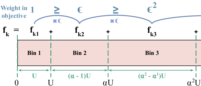
Fig. 6 shows the key idea behind our one-shot geometric binner. If we consider each allocation as the sum of contributions from different, geometrically-sized bins, we can use $\epsilon$-weighting per bin to incentivize the optimization to allocate more from the smaller bins. The resulting formulation is:

$$\mbox{\sf GeoBinning}(\mathcal{E},\mathcal{D},\mathcal{P})\leavevmode\nobreak\ \triangleq \arg\max_{\mathbf{f}}\sum_{k\in\mathcal{D}}\leavevmode\nobreak\ {\color[rgb]{0.5,0,0}\definecolor[named]{pgfstrokecolor}{rgb}{0.5,0,0}\sum_{\mbox{bins}\leavevmode\nobreak\ b}\epsilon^{b-1}f_{kb}}$$ (4)

s.t. $$f_{k}=\sum_{\mbox{bins}\leavevmode\nobreak\ b}f_{kb}, \forall k\in\mathcal{D}$$

$$f_{k1}\leq U, \forall k\in\mathcal{D}$$

$$f_{kb}\leq U(\alpha^{b-1}-\alpha^{b-2}), \forall b>1,\forall k\in\mathcal{D}$$

$$\mathbf{f}\in{\sf FeasibleAlloc}(\mathcal{E},\mathcal{D},\mathcal{P}).$$

The geometric binner (Eqn. 4):

• Applies to various bin choices beyond the geometric ones we used here. We use a similar intuition from equi-depth binning in databases [32] to show in §3.3 that we can choose bin boundaries to improve fairness.

• Offers the same fairness guarantee as SWAN [30] when using the same (geometric) bins. GeoBinning allocates rates within an $\alpha$ ratio of the optimal max-min fair rates for any demand.

  Theorem 2.

  Eqn. 4 assigns resources to a demand $k$ in bin $b$ only if it has assigned demand $k$ the full rate from all of the larger-weighted bins.

  Proof Sketch.

  Assume otherwise: Eqn. 4 has assigned a non-zero rate to some demand $k$ in some bin $b$ without assigning the full rate from some other bin $j<b$. Then, we can move some $\delta$ rate from bin $b$ to $j$ and not violate any constraints yet improve the objective value. ∎

  We can combine Theorem 2 with the proof technique of Theorem 1 to prove Eqn. 4 will allocate the same rates as Eqn. 3, so the approximation ratio proof from [30] applies directly.

• Lets users adjust $\alpha$ to balance the trade-off between fairness approximation guarantee and the solver time.

• Is less likely to run into precision issues compared to Eqn. 2 since there are fewer bins than demands.

• Requires no sorting constraints unlike Eqn. 2.

• Is only slightly larger in size compared to each of the optimizations in Eqn. 3 (see §F for more details). The key difference is that we can now run one LP instead of many. The one-shot optimization is empirically faster, likely due to redundant computation between the LPs in the sequence of optimizations in Eqn. 3.

3.2 Multi-path Waterfilling

We also generalize the classical waterfilling algorithm for max-min fair allocation over multiple resources. We present parallelizable combinatorial algorithms (and not optimizations) with better empirical performance compared to §3.1 but weaker fairness guarantees.

Waterfilling is a well-known method that applies to scenarios where all the demands are unconstrained and require resources on exactly one path [36]. Under these conditions, we can achieve max-min fairness by visiting resources in the ascending order of their fair share and splitting their capacities fairly among the demands [67] (see Alg. 1)

We extend this approach to constrained demands by adding a virtual edge with a capacity equal to the requested rate for each demand. This augmented topology ensures that demands receive at most what they asked for. For small requests, the virtual edge becomes the bottleneck and limits the allocation.

Input: $\boldsymbol{\mathit{\Gamma}}$ where $\boldsymbol{\mathit{\Gamma}}[e,k]$ is the weight of single-path demand $k$ on link $e$.

Input: $\mathbf{c}$: link capacity vector.

Output: $\mathbf{f}$: max-min rate allocation vector.

1

$\mathcal{D}_{a}\leftarrow[0,\dots,K-1]$

  initial list of active demands

$\mathbf{f}\leftarrow\mathbf{0}$

  initial rate vector

2

3while $\lvert{\mathcal{D}_{a}}\rvert>0$ do

       $\mathbf{n}\leftarrow\boldsymbol{\mathit{\Gamma}}\mathbf{1}$

        total weight per link

       $\mathbf{\boldsymbol{\zeta}}\leftarrow\frac{\mathbf{c}}{\mathbf{n}}$

        vector division, fairshare per link

       $e\leftarrow\mathop{\mathrm{arg\,min}}\leavevmode\nobreak\ \leavevmode\nobreak\ \mathbf{\boldsymbol{\zeta}}$

        link with minimum fair share

       $\mathcal{D}_{e}\leftarrow\{k:\boldsymbol{\mathit{\Gamma}}[e,k]>0\}$

        active demands on link $e$

4       foreach $k\in\mathcal{D}_{e}$ do

             $\mathbf{f}[\mathcal{D}_{a}[k]]\leftarrow\boldsymbol{\zeta}[e]\boldsymbol{\mathit{\Gamma}}[e,k]$

              fix to weighted fair share

5             foreach $l:\boldsymbol{\mathit{\Gamma}}[l,k]>0$ do

                   $\mathbf{c}[l]\leftarrow\mathbf{c}[l]-\mathbf{f}[\mathcal{D}_{a}[k]]$

                    deduct allocations

6                  

7             end foreach

8            

9       end foreach

      $\mathbf{c}\leftarrow\mathbf{c}[\setminus\{e\}]$

        remove link $e$

       $\boldsymbol{\mathit{\Gamma}}\leftarrow\boldsymbol{\mathit{\Gamma}}[\setminus\{e\};\setminus\mathcal{D}_{e}]$

        remove link $e$ and its demands

       $\mathcal{D}_{a}\leftarrow\mathcal{D}_{a}\setminus\mathcal{D}_{e}$

        update set of active demands

10      

11 end while

return $\mathbf{f}$

Algorithm 1 Waterfilling algorithm to compute single-path weighted max-min fair rates.

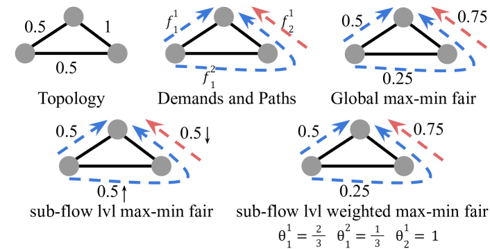
It is harder to generalize waterfilling to multi-path settings because the local max-min fair allocation at individual resources is not globally fair. Fig. 7 shows a simple example where the blue demand — which has access to more paths — must receive a locally unfair share on the common link in order to produce a globally max-min fair solution. We next modify waterfilling to produce approximate, globally max-min fair rates in the general multi-resource setting.

(a) Global and Local (per-link) max-min fairness are different.

	# iteration $t\longrightarrow$
$\theta^{1}_{1}$	$\frac{1}{2}$	$\frac{3}{5}$	$\frac{7}{11}$	$\frac{15}{23}$	$\frac{31}{47}$	$\frac{63}{95}$	$\ldots$	$\frac{2}{3}$
$\theta^{2}_{1}$	$\frac{1}{2}$	$\frac{2}{5}$	$\frac{4}{11}$	$\frac{8}{23}$	$\frac{16}{47}$	$\frac{32}{95}$	$\ldots$	$\frac{1}{3}$
$\theta^{1}_{2}$	$1$	$1$	$1$	$1$	$1$	$1$	$\ldots$	$1$
$f^{1}_{1}$	$\frac{1}{2}$	$\frac{1}{2}$	$\frac{1}{2}$	$\frac{1}{2}$	$\frac{1}{2}$	$\frac{1}{2}$	$\ldots$	$\frac{1}{2}$
$f^{2}_{1}$	$\frac{1}{3}$	$\frac{2}{7}$	$\frac{4}{15}$	$\frac{8}{31}$	$\frac{16}{63}$	$\frac{32}{127}$	$\ldots$	$\frac{1}{4}$
$f^{1}_{2}$	$\frac{2}{3}$	$\frac{5}{7}$	$\frac{11}{15}$	$\frac{23}{31}$	$\frac{47}{63}$	$\frac{95}{127}$	$\ldots$	$\frac{3}{4}$

(b) AW’s weight multipliers and allocations converge to global max-min fair allocation.

Figure 7: An example to illustrate the difficulty in extending waterfilling to multi-path settings and how our AdaptiveWaterfiller effectively tackles the issue. Waterfilling (single-path) computes local fair shares and is ineffective in multi-path settings as it ignore the dependencies between different paths of a single demand.

ApproxWaterfiller (or aW): For each demand, aW creates several “subdemands”, each going through one of the demand’s paths. Subdemands of each demand pass through a shared virtual edge to ensure the algorithm does not allocate more than the requested rate. We then use waterfilling to assign rates to these subdemands. This algorithm simply ignores the coupling between multiple paths and does not reach global max-min fair rates, but we use it as the starting point to generalize waterfilling. As a solution, it is fast, and we also use a variant of Alg. 1 to speed it up further (Alg. 2).

The new algorithm simplifies Alg. 1 by retaining the initial order of the links in subsequent iterations. In each iteration, it only recomputes the fair share for the link under consideration and fixes the rates for the demands bottlenecked by that link. It is approximate (even in the one-path case [5, 54]) but is faster and more parallelizable.

Global max-min fairness assigns lower rates to subdemands that are on congested paths but their corresponding demand can get enough allocation from its other paths. For example, the blue demand in Fig. 7(a) should receive a lower allocation on the path through the congested link. Intuitively, the allocator can get closer to global max-min fair assignments by moving each demand’s allocation from more congested paths to less congested ones. We can achieve this by iteratively seeking more rates from subdemands that have received higher rates (i.e., on less-contended paths) in previous iterations.

Input: $\boldsymbol{\mathit{\Gamma}}$ where $\boldsymbol{\mathit{\Gamma}}[e,k]$ is the weight of single-path demand $k$ on link $e$.

Input: $\mathbf{c}$: link capacity vector.

Output: $\mathbf{f}$: max-min rate allocation vector.

1

${\mathbf{f}}\leftarrow\boldsymbol{\infty}$

  initial max-min rate set to $\infty$

$\mathbf{n}\leftarrow\boldsymbol{\mathit{\Gamma}}\mathbf{1}$

  total weight per link

$\mathcal{L}\leftarrow\mathop{\mathrm{arg\,sort}}\leavevmode\nobreak\ \frac{\mathbf{c}}{\mathbf{n}}$

  vector division, sort links in ascending order

2 foreach $e\in\mathcal{L}$ do

       $\mathcal{D}_{e}\leftarrow\{k:\boldsymbol{\mathit{\Gamma}}[e,k]>0\}$

        demands on link $e$

3       while $\mathcal{D}_{e}\neq\emptyset$ do

             $\zeta\leftarrow\frac{\mathbf{c}[e]}{\sum_{k\in\mathcal{D}_{e}}\boldsymbol{\mathit{\Gamma}}[e,k]}$

              fair share of link $e$

4             $\mathcal{B}\leftarrow\{k\in\mathcal{D}_{e}:\mathbf{f}[k]<\zeta\boldsymbol{\mathit{\Gamma}}[e,k]\}$

5             if $\mathcal{B}=\emptyset$ then if no flows bottlenecked elsewhere,

                   $\mathbf{f}[\mathcal{D}_{e}]\leftarrow\zeta\boldsymbol{\mathit{\Gamma}}[e,\mathcal{D}_{e}]$

                    fix rate to weighted share.

6                   break

7                  

8            else  otherwise, remove those bottlenecked elsewhere.

9                   $\mathbf{c}[e]\leftarrow\mathbf{c}[e]-\sum_{k\in\mathcal{B}}\mathbf{f}[k]$

10                   $\mathcal{D}_{e}\leftarrow\mathcal{D}_{e}\setminus\mathcal{B}$

11             end if

12            

13       end while

14      

15 end foreach

return $\mathbf{f}$

Algorithm 2 Our Approx. Waterfilling algorithm to compute single-path weighted max-min fair rates.

AdaptiveWaterfiller (or AW): Motivated by this intuition, AW uses a weighted version of aW (using Alg. 1 or Alg. 2) and adjusts the input weights ($\boldsymbol{\mathit{\Gamma}}$) to seek more rate from subdemands on less congested paths.

Let $\theta^{p}_{k}$ be the weight multiplier for the subdemand of demand $k$ on path $p$. AW initializes these multipliers as $\theta^{p}_{k}=\frac{1}{\|\{p\in\mathcal{P}_{k}\}\|}$. In each iteration, AW first computes $\boldsymbol{\mathit{\Gamma}}$ directly from $\theta$. $\boldsymbol{\mathit{\Gamma}}[e,k_{p}]$ is the weight of the subdemand $k_{p}$ (demand $k$ on path $p$) on link $e$. Following the definition, $\boldsymbol{\mathit{\Gamma}}[e,k_{p}]=\theta^{p}_{k}\leavevmode\nobreak\ \mathbbm{1}\left[{e\in p}\right]$. AW then invokes one of the waterfilling algorithms with these weights $\boldsymbol{\mathit{\Gamma}}$. For iteration $t+1$, AW sets $\theta^{p}_{k}(t+1)=\frac{f^{p}_{k}(t)}{\sum_{p}f^{p}_{k}(t)}$ where $f^{p}_{k}(t)$ is the rate demand $k$ obtains from path $p$ in iteration $t$. We show how multipliers and rates evolve in our example in Fig. 7(b).

AW converges when $\theta^{p}_{k}(t+1)=\theta^{p}_{k}(t)$. We can prove that adapting weight multipliers gets close to global max-min fairness: we say a rate assignment in the multi-path setting is bandwidth-bottlenecked if for all demands $k$, (i) each of its subdemands $f^{p}_{k}$ is bottlenecked on some link $l$, and (ii) $f_{k}\geq f_{j}$, for all demands $j$ that have any subdemand on any such link $l$. We prove in §D.1 that:

Theorem 3.

If the adaptive waterfiller converges, it converges to a bandwidth bottlenecked assignment.

We prove the global max-min fair allocation is bandwidth-bottlenecked (see §D.2). The converse is not true — not all bandwidth-bottlenecked allocations are max-min fair. However, the set of bandwidth-bottlenecked allocations is significantly smaller than the set of all feasible allocations. We also prove that AW converges when its assignment is bandwidth-bottlenecked (i.e., it stops iterating). Empirically, AW’s allocations stabilize within $5$ – $10$ iterations on average (§4.4).

Adaptive waterfiller produces allocations that belong to a constrained set containing the optimal max-min fair rates. It is slower than approximate waterfiller because it iterates and updates weight multipliers. It is faster than the Geometric Binner as it does not solve an LP. Users can tune the maximum number of iterations to trade-off between fairness and speed.

3.3 Combinations and Extensions

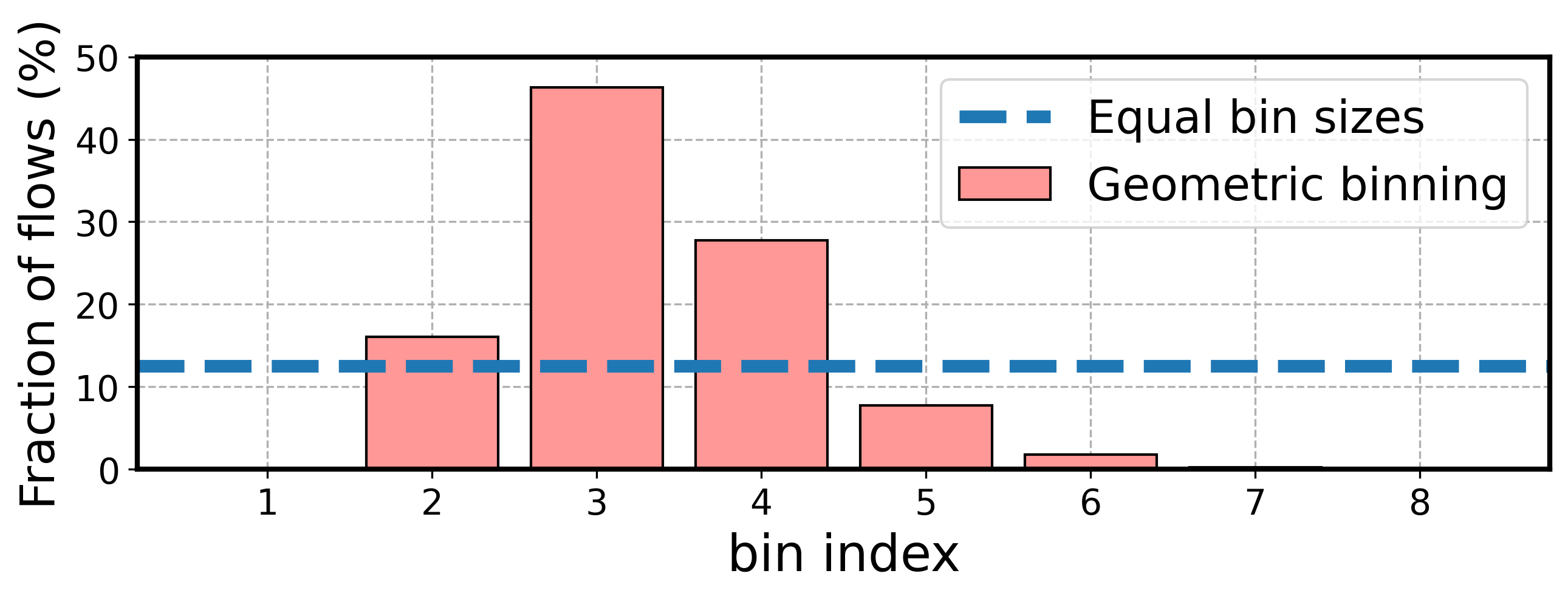
Empirically, we find that the geometric binner (§3.1) is fairer than what its worst-case guarantee suggests (recall, we prove the rates will be within $[\alpha^{-1},\alpha]$ times the optimal max-min fair rate). We can attribute most of the unfairness to bins that happen to contain many demands (Fig. A.5): can we set the bin boundaries differently to improve fairness?

We use the generalized waterfillers (§3.2) — which are fast but lack worst-case guarantees — to set bin boundaries in a way that spreads demands more uniformly across bins:

Equi-depth Binner (or EB) applies GeoBinning (Eqn. 4) with a few changes: it uses the rate allocation from AdaptiveWaterfiller to approximate the order across demands; distributes demands more uniformly over bins; and finds the bin boundaries as part of the optimization. Specifically, EB divides demands $\mathcal{D}$ into $N_{\beta}$ equi-sized sets ($\mathcal{D}_{1}\ldots\mathcal{D}_{n}$) based on their increasing order of rates from AW. In EB, the demands in a set $D_{b}$ only receive rates from one bin with index $b$. EB dynamically chooses bin boundaries: $\forall k\in D_{b},{\ell}_{b-1}\leq f_{k}<{\ell}_{b}+s(b)$ where $s(b)$ is a small constant that helps reducing the impact of inaccuracies from AW. We provide a more formal definition of EB in §E.

EB is slower than GB and AW because it executes both but we expect it to be fairer than GB — it spreads demands more uniformly across bins. We empirically confirm this hypothesis. It is hard to formally analyze EB but we suspect it also offers tighter worst-case guarantees. This is subject for future work.

Extensions: We did not explicitly account for weighted max-min fairness (e.g., $w_{k}$ in §2.1) when describing our one-shot optimization. This extension is straightforward. For example, we can replace the first constraint in the geometric binner (GB) in Eqn. 4 with $f_{k}/w_{k}=\sum_{\text{bins}\leavevmode\nobreak\ b}f_{kb}$. Algorithm 2, which we use in our generalized waterfillers in §3.2, already supports weights. We compute the per-edge per-subdemand weighted routing matrix as $\boldsymbol{\mathit{\Gamma}}[e,k_{p}]=w_{k}\theta_{k}^{p}\mathbbm{1}\left[{e\in p}\right]$.

We have also omitted the heterogeneous utilities, different resource consumption scales, and other affine functions in our model (§2.1) when describing the solutions. These extensions are also straightforward and we show them in §A. The key is to appropriately manipulate the constraints that determine when an allocation is feasible (FeasibleAlloc, Eqn. 5).

4 Evaluation

Implementation. We implemented Soroush in Python and C# using Gurobi 9.1.1 [27] as the solver.

Summary of results. We apply Soroush to traffic engineering (TE) and cluster scheduling (CS). We show Soroush captures the trade-off between speed, fairness, and efficiency. We also show the results from integrating Soroush with Azure’s production TE system where it reduces the run-times by up to $5.4\times$ without any impact on efficiency and fairness.

In TE, all the allocators in Soroush are faster than both the optimal algorithm by Danna et al. [17] (referred to as Danna) and the more practical $\alpha$-approximate SWAN [30]. Soroush contains algorithms that match or exceed the efficiency or fairness of these methods while running orders of magnitude faster. Soroush can also trade-off (a little) fairness and efficiency for up to $3$ orders of magnitude speed up.

Our solution scales to one of the largest WAN topologies (over $1000$ nodes and $1000$ edges), which is significantly larger than those in [17, 34, 30, 75, 10] and matches the size of topologies in [4]. We also analyze the sensitivity of Soroush to demand variations and other relevant inputs.

In CS, we show Soroush outperforms two variants of Gavel [56]. Our Equi-depth binner (EB) has the same fairness and efficiency as the optimal variant of Gavel (the one with waterfilling), but is $2$ orders of magnitude faster.

4.1 Benchmarks and Metrics

Benchmarks. We use state-of-the-art solutions in both WAN-TE and CS as benchmarks to evaluate Soroush:

WAN-TEs. We use Danna [17], SWAN [30], and a modified version of the k-waterfilling algorithm [36] as benchmarks. We also provide limited comparisons with B4 [34] for completeness (see §4.2). The k-waterfilling algorithm only applies to single-path, infinite-demand scenarios — we extend it to multi-path, demand-constrained cases. We tune each benchmark for maximum speed (see §G.1). Following [30], we set $\alpha=2$ for SWAN and GB unless mentioned otherwise.

CS. We compare with two variants of Gavel [56], the state-of-the-art max-min fair allocator in CS (with and without waterfilling). We use Gavel’s public implementation.

Topology	# Nodes	# Edges
WANLarge	$\sim$1000s	$\sim$1000s
WANSmall	$\sim$100s	$\sim$1000s
Cogentco	197	486
UsCarrier	158	378
GtsCe	149	386
TataNld	145	372

Table 4: Topologies used for the evaluation of Soroush.

Metrics. We use the following metrics for comparisons:

Fairness. We report fairness of a particular allocation ($\mathbf{f}$) as its distance from the optimal max-min fair allocation ($\mathbf{f}^{*}$). For fairness distance, we use the $q_{\vartheta}$ metric [46, 47]. This metric is resilient to numerical instability and is computed as $\min\big{(}\frac{\max(f_{k},\vartheta)}{\max(f^{*}_{k},\vartheta)},\frac{\max(f^{*}_{k},\vartheta)}{\max(f_{k},\vartheta)}\big{)}$ for a given demand $k$. We report the geometric mean of $q_{\vartheta}$ across all the demands as the overall fairness measure (the geometric mean is less sensitive than the arithmetic mean to outliers). For our evaluations, we use $\vartheta=0.01\%$ of the resource (link or GPU) capacities.

Efficiency. We measure efficiency in TE as the total rate allocated to flows relative to Danna (i.e., $\frac{e}{e_{danna}}$). For CS, we measure the effective throughput which is the progress rate of a job given an allocation. We report CS efficiency relative to Gavel (i.e., $\frac{e}{e_{gavel}}$).

Runtime. In most cases, we report speed up (i.e., relative runtime compared to a baseline $\frac{s_{baseline}}{s}$). Our runtimes consist of the time each algorithm needs to compute the allocations. We measure runtimes on an AMD Operaton 2.4GHz CPU (6234) with 24 cores and 64GB of memory.

() High Load (scale factor $\in$ {64, 128})

(a) Medium Load (scale factor $\in$ {16, 32})

(b) Light Load (scale factor $\in$ {1, 2, 4, 8})

Figure 8: The fairness vs speed trade-off across different approaches. As in [4], we use the scale-factor to denote the level of load. We observe even the slowest algorithm in Soroush is faster than SWAN and Danna. While 1-waterfilling is faster than most of the algorithms in Soroush, it has to sacrifice much more in terms of fairness (it is $30\%$ less fair than Danna in the high load case).

(a) High Load (scale factor $\in$ {64, 128})

(b) Medium Load (scale factor $\in$ {16, 32})

(c) Light Load (scale factor $\in$ {1, 2, 4, 8})

Figure 9: The efficiency of Soroush’s algorithms and our benchmarks. We report numbers relative to Danna. Empirically, Soroush Pareto-dominates SWAN, 1-waterfilling, and Danna on the efficiency, agility, and fairness. In (c), the error bar is small because of light load — most solutions can satisfy all the demands (fairness is also close to one for most algorithms in these cases.)

4.2 WAN Traffic Engineering

Experiment Setup. Table 4 summarizes the topologies in our evaluation. We show the results for both Azure’s production WAN topology and the topologies from the Topology Zoo [1]. We use K-shortest paths [73] to find the paths between node pairs (K=16 unless mentioned otherwise).

For topologies from Topology Zoo, we generate traffic using Poisson [6], Uniform, Bimodal, and Gravity [6, 62] distributions. We follow [4] and generate traffic at different scale factors. Our traffic spans a range of loads: light (scale factors {1, 2, 4, 8}), medium ({16, 32}), and high ({64, 128}). At higher loads, more flows compete for traffic than at medium or light loads. We report results of over $640$ experiments, which capture different traffic and topology combinations.

Comparison to benchmarks (Fig. 9 and 9). All algorithms in Soroush are faster than SWAN and Danna (Fig. 9). Each approach is in a different color in this figure, and each point corresponds to a single traffic demand on a single topology. The plot also shows the mean and standard deviations along the fairness and speedup axes.

We see the trade-off across these different max-min fair resource allocators: (a) Danna is optimal but also by far the slowest (on average taking $4.3\times$ longer than the second slowest algorithm, SWAN, under high-load); (b) 1-waterfilling is the fastest of the baselines but does not consider flow-level fairness ($30\%$ less fair than Danna on average but 4 orders of magnitude faster); (c) SWAN sits somewhere in between. It is faster than Danna (solves fewer optimizations), but slower than 1-waterfilling (1-waterfilling does not solve any optimization). It is fairer than 1-waterfilling but unlike Danna does not achieve optimal max-min fairness; (d) Soroush empirically Pareto-dominates these baselines as each of its algorithms provide a different point on the trade-off space.

Our algorithms are most effective under high loads (arguably, speed and fairness matter most). Soroush’s Geometric Binner (GB) is faster than SWAN by $4.5\times$ on average ($6\times$ in the $90^{th}$ percentile) because it only solves a single optimization. GB also has worst-case fairness guarantees. The Equi-depth Binner (EB) is faster than SWAN, slightly slower than GB, and fairer than both. Soroush’s Approximate Waterfiller is even faster than 1-waterfilling (by an order of magnitude) with the same flow-level fairness. Soroush’s Adaptive Waterfiller improves fairness ($19\%$ higher on average) at a slight speed reduction (still $21.4\times$ faster than SWAN on average).

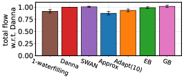
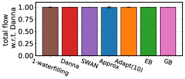
Fig. 9 compares the efficiency of different methods. Under low loads, all schemes are comparable. The differences become evident at higher loads, where EB is approximately as efficient as Danna. GB and SWAN are more efficient, likely because they sacrifice fairness.

(a) Fairness vs Run-time

(b) Efficiency wrt Danna

Figure 10: The empirical Pareto-dominance of Soroush over all of our baselines on an example topology (Cogentco) and an example workload with $64\times$ scale factor. The size of the markers in (a) are in proportion to the efficiency of each algorithm — we report exact comparisons in (b).

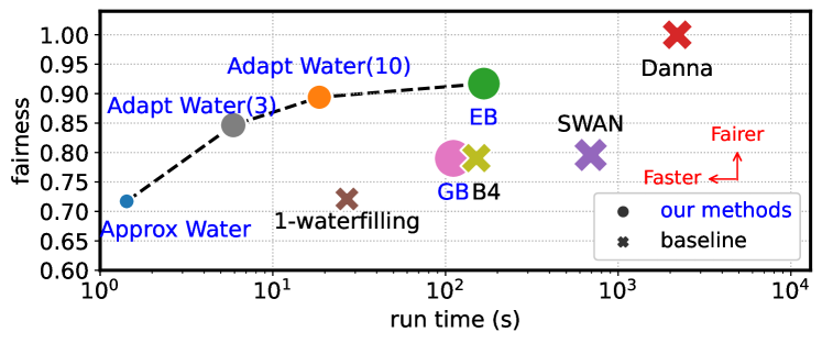
We can see these differences more clearly when we focus on a single topology and workload in Fig. 10. Soroush’s allocators Pareto-dominate other approaches. The Approximate Waterfiller, Adaptive Waterfiller (number of iterations = 3 and 10), and EB are faster than SWAN and Danna. Adaptive Waterfiller and EB are also fairer than SWAN while having comparable efficiency. Operators can use GB to get strong worst-case guarantees (at the cost of reduced fairness). B4 [34]’s TE algorithm is just as fast and fair as GB (albeit slightly less efficient) but does not have fairness guarantees. Note that we can control the fairness and runtime of GB by tuning $\alpha$, whereas we can not control either in B4.

In summary, in settings where Danna is impractical, Soroush outperforms other TE algorithms (SWAN, 1-waterfilling, B4). Depending on the requirements, users can opt for Adaptive or Approximate Waterfillers, or EB (or GB if fairness guarantees are important). They can also customize the parameters in each allocator to further tune the balance.

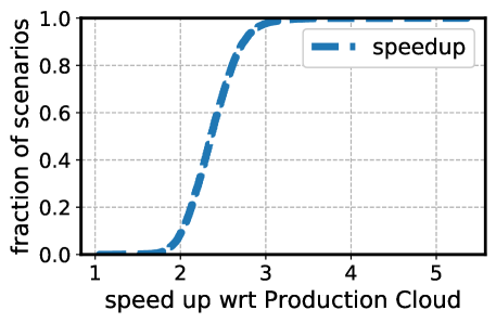
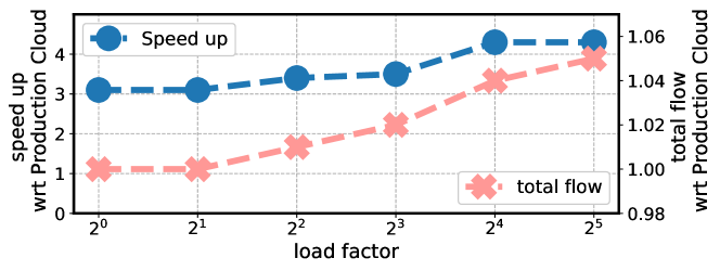
Production deployment (Fig. 12). We have successfully deployed Soroush in the production TE pipeline of Azure. Microsoft opted for GB as it has the same fairness guarantees as their existing TE solver. Fig. 11(a) shows cumulative density function (CDF) of the relative speed up of Soroush compared to the provider’s previous allocator. These measurements are over a month-long deployment in a WAN with thousands of nodes. Soroush reduces the run-time on average by $2.4\times$ (up to $5.4\times$) without impacting fairness or efficiency.

We compare Soroush with the previous allocator on production demands at different loads (Fig. 11(b)). Soroush’s speedup increases with the load because the previous iterative solver invokes more optimizations at higher loads. Soroush’s efficiency also increases because its $\epsilon$-trick can exploit minor fairness violations to improve efficiency. In all cases, Soroush is within 1% of the previous solver’s fairness.

(a) Speedup

(b) Impact of load

Figure 11: Results from deploying Soroush in production. (a) Month-long measurements show substantial speedup with no impact on efficiency or fairness compared to the provider’s previous max-min fair allocator. (b) Using production traces, we show the benefit of Soroush improves as loads [4] increase.

Figure 12: Impact of solver runtimes on fairness when demands change. SWAN can not react to the new demands quickly and faces another 10% reduction in fairness whereas EB can keep track of the changes. These results are on Cogentco following NCFlow’s change distribution [4] on medium load traffics.

(a) Fairness vs Run-time

(b) Efficiency wrt Gavel w-waterfilling

Figure 13: Trade-off between efficiency, fairness, and speed in CS on an example scenario (with 8192 jobs). (a) shows the fairness vs run-time behavior of the different approaches; (b) shows the efficiency relative to the Gavel w waterfilling. Empirically, Soroush Pareto-dominates both variants of Gavel.

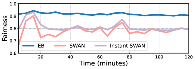
Tracking Changing Demands (Fig. 12). We evaluated each method on a sequence of traffic, arriving every five minutes (a window), starting from a medium load traffic demand. Our methodology is the same as NCFlow [4]. In this scenario, SWAN needs two windows to compute each allocation – it only computes allocations for half of the demands. This results in up to 10% reduction in fairness compared to an instant SWAN (a hypothetical scheme that computes the allocation instantly). However, EB reacts to changes quickly and meets all the deadlines. In general, SWAN’s inability to keep track of demands leads to even higher unfairness than EB (relative to what we reported in Fig. 9). Also, as we move from medium to high load, we expect the difference to be more as SWAN is even slower and needs to solve more optimizations.

(a) Convergence of the Adaptive Waterfiller

(b) Impact of the number of bins on the fairness

(c) Impact of the number of bins on the efficiency

Figure 14: Convergence and sensitivity analysis. (a) Adaptive Waterfiller empirically converges within 5 – 10 iterations. (b, c) The number of bins controls the trade-off between fairness and efficiency in EB and GB (fewer bins lead to higher efficiency and lower fairness). Results are on the Cogentco topology and Gravity traffic distribution (scale factor = 64). (see Fig. A.3 for Poisson)

4.3 Cluster Scheduling

Experiment Setup. We generate job requests from Gavel’s job generator: we consider $3$ types of GPUs (V100, P100, K80) and uniformly sample jobs from the $26$ different job types available in Gavel (see §G.2). Jobs are heterogeneous: they require a different number of workers (which we derive from the Microsoft public trace [3]) and have different priorities (which we sample uniformly from the set $\{1,2,4,8\}$).

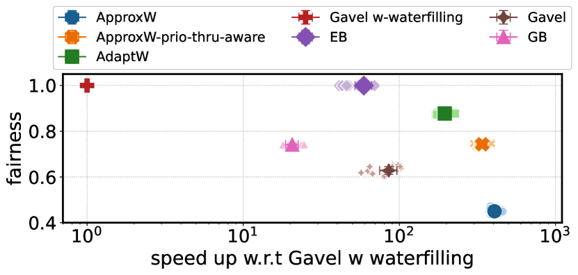
Comparison to benchmarks. We report results on over 40 different scenarios, which capture different number of available GPUs and competing jobs (see §G.2 for more details). Our results match our observations from WAN-TE; Soroush Pareto-dominates both Gavel and Gavel with waterfilling. We present these results in Fig. A.2 in §G.2 for space.

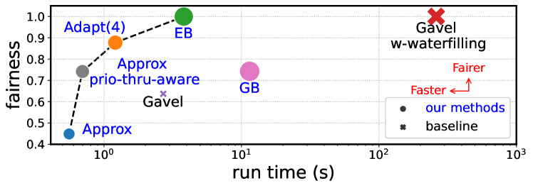
We provide further insight into Soroush’s performance through an example scenario where 8192 jobs compete for resources (Fig. 13). Adaptive Waterfiller outperforms standard Gavel in fairness, efficiency, and speed. For CS, GB is slower than Gavel but fairer (more than $10\%$) and more efficient (more than $30\%$). We can augment Gavel with waterfilling [56] to improve it, but with a substantial slowdown. In contrast, EB provides comparable fairness and efficiency as Gavel with waterfilling and is $\sim$ 2 orders of magnitude faster.

4.4 Convergence and Sensitivity Analysis

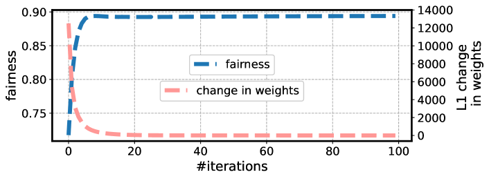
Convergence. We empirically evaluate the convergence of the Adaptive Waterfiller. In §D, we proved the algorithm in §3.2 only converges to and stops if it finds a bandwidth-bottlenecked allocation but may not converge if it does not find one. We empirically find that Adaptive Waterfiller always converges. Fig. 14(a) shows how its weights and fairness properties change with the number of iterations: the weights stabilize after 5 iterations.

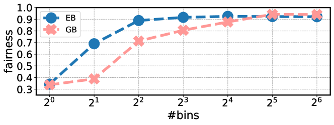
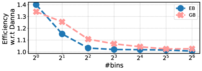
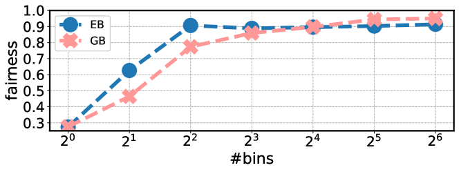
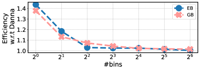
Impact of number of bins. Fig. 14(b) and 14(c) show fairness and efficiency of binners (GB/EB) for different number of bins. Soroush uses this parameter to tune the trade-off between efficiency, fairness, and run-time. Using more bins increases fairness because the number of demands within each bin decreases but at the cost of higher run-time (more variables in the optimization). EB is fairer than GB for up to 16 bins because GB suffers from bin-imbalance. However, GB does not incur bin-imbalance for $\geq 32$ bins and both methods have roughly the same fairness. The slightly lower fairness of EB is due to Adaptive Waterfiller making small mistakes when estimating the order of rates and influencing EB’s binning.

4.5 Other Experiments

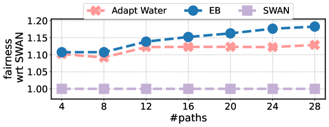
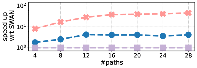
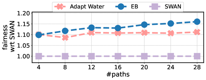
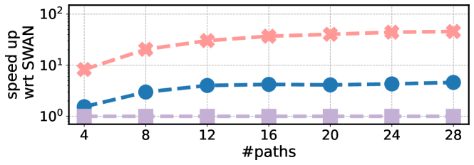
Impact of number of paths. We explore how sensitive our solutions are to the number of paths by varying this parameter and comparing our fairest methods (i.e., Adaptive Waterfilling and EB) to SWAN (Fig. 16). Increasing the number of paths improves the benefit of Soroush in both speedup and fairness. With more paths, each optimization of SWAN becomes more expensive, while Adaptive Waterfiller as well as EB can exploit path diversity better to achieve higher fairness.

Figure 15: Increasing the number of paths improves the fairness and speedup of Soroush compared to SWAN. Results are on the Cogentco topology and Gravity traffic distribution (scale factor = 64). (see Fig. A.4 for Poisson)

Figure 16: Impact of topology size. Soroush’s speed up relative to SWAN improves with the size of the topology.

Impact of topology size. The benefit of Soroush’s allocators increases with the topology size (Fig. 16): SWAN needs to solve more optimizations for larger topologies while Soroush solves a fixed number of optimizations (=1 for EB/GB and =0 for adaptive waterfilling).

Comparison to NCFlow and POP. NCFlow [4] and POP [55] decompose the resource allocation problem to scale but do not directly address max-min fairness [65]. NCFlow only maximizes the total flow, and the authors mention in the paper that it is hard to extend it to max-min fairness objective [4]. Similarly, POP maximizes total flow and maximum concurrent flow (i.e., the smallest fractional allocation) but does not provide any results on max-min fairness. To understand how POP compares to Soroush, we adapt both SWAN and Soroush to use it. We randomly divide demands (with client splitting as needed per POP’s guidelines) among different partitions and run SWAN or Soroush in parallel on each partition (Fig. 17, extended evaluation in §G.3).

We use GB to ensure a fair comparison to SWAN: it has the same theoretical guarantees, is more than $10\times$ faster, and maintains the same level of fairness. When we apply POP to SWAN, we lose the worst-case guarantee [53] and have to sacrifice over $10\%$ in fairness to achieve the same speed as Soroush. We also observe that applying POP to Soroush results in the same fairness as SWAN for the same number of partitions (but is also substantially faster).

Figure 17: Impact of POP [55]. The results are on 3 randomly generated traffic, following Poisson distribution with a scale factor 64, on the Cogentco topology. Consistent with POP, we use client splitting (ratio$=0.75$) for this traffic distribution. ["X" indicates that POP is not used, and "Numbers" = number of POP partitions.]

5 Discussion

Soroush allows operators to adjust the trade-off between fairness, speed, and efficiency. We focus on multi-path allocations but our solutions apply to single-path settings too [5, 54]. Under this setting, our experiments show the Approximate Waterfiller is an order of magnitude faster than the fastest single-path allocator with only a slight decrease in efficiency. We defer the following to future work:

Other fairness metrics. Soroush does not apply to other, less commonly used, fairness metrics [33, 11, 12].

Other problem domainss. Soroush applies to any graph-based resource allocation problem which seeks to achieve max-min fairness. We demonstrate significant benefit of Soroush using examples from CS and WAN-TE. To use Soroush in other domains [71, 5, 36, 64, 50, 43, 24, 54], users need to model the additional constraints in our graph model. We aim to provide tools to simplify this in future work.

Distributed extension. Soroush applies to centralized resource allocation problems. Our future work aims to extend it to distributed settings [36, 61, 74, 70].

6 Related Work

TE and CS resource allocation. Prior approaches to both TE and CS aim to produce fast and efficient allocations [30, 56, 34, 17, 59, 36, 23, 16, 37, 14, 42]. In §4, we show Soroush outperforms the sate-of-the-art in multi-resource max-min fair allocation (SWAN, Danna, B4, waterfilling, and Gavel).

Prior work employs ML in TE [68, 58, 72] to optimize objectives that are already solved using a single LP (e.g., max flow). These objectives are either convex or quasi-convex [58]. However, the exact from of max-min fairness is sequential and we are unaware of any work that considers end-to-end training on a sequence of LPs. In fact, it may be more tractable for ML methods to learn our GB which is a single LP. Applying ML to further speed up Soroush is an interesting future direction.

Recent work [4, 55] uses decomposition techniques to scale resource allocation problems. However, they focus on simpler objectives such as max flow or max concurrent flow that require single LPs and do not explicitly support max-min fairness. Extending NCFlow to max-min fairness is non-trivial as the authors mentioned [4]. We have extended POP to support max-min fairness and empirically compare it with Soroush. Our results show POP’s performance depends on the traffic distribution, whereas Soroush works consistently well. POP also does not have worst-case fairness guarantees [53], whereas Soroush has allocators that do (GB).

Algorithms for computing max-min fair rates. Prior work has expanded our understanding of max-min fair resource allocation [57, 60]. These are largely theoretical and do not provide a practical and fast solution. Bandit-based solutions [9] lack worst-case guarantees and do not allow users to control the trade-off between fairness, efficiency and speed.

7 Conclusion

Soroush enables fast max-min fair resource allocation for graph-based problems such as traffic engineering and cluster scheduling. It provides a suite of allocators that Pareto-dominate state-of-the-art in both of these domains. Some of the allocators in Soroush have theoretical guarantees, and all of them have parameters for users to control the trade-offs. We have deployed Soroush in Azure’s WAN traffic engineering pipeline. Future work can explore other applications and other notions of fairness.

Acknowledgements: We thank Ymir Vigfusson and the anonymous reviewers for their feedback on this paper. We also thank Luis Irun-Briz for his support of this work. This material is based upon work supported by Microsoft and the U.S. National Science Foundation under grant No. CNS-1901523.

Figure A.1: Sorting Network Example.

Appendix A Max-min fair allocation optimization

Term	Meaning	CS	WAN-TE
$\mathbf{w}$	inverse of coefficient vector in the objective of fair(.) where $w_{k}$ indicates the weight for the $k$-th demand and encodes the desired proportional max-min fair allocations.	priority of job $k$ (In [56] = user specified priority $\times$ effective average throughput $/$ number of workers)	priority of different services (e.g., search and ads)
$q^{p}_{k}$	the utility obtained by demand $k$ when assigned 1 unit on path $p$.	progress rate of the $k$-th job when assigned 1 unit on server $p$	$=1$
$r^{e}_{k}$	capacity consumed on resource $e$ (i.e., link or GPU) when allocating 1 unit to demand $k$	capacity consumed by job $k$ from resource $e$ (CPU, GPU or memory)	$=1$
$c_{e}$	capacity of resource $e\in\mathcal{E}$	capacity of CPU, GPU or any other resources on a server	capacity of link $e$
$d_{k}$	the resource requested by the $k$-th demand	job $k$’s requested duration of time ($=1$ in [56])	flow $k$’s requested rate
$f_{k},f^{p}_{k}$	$f_{k}:$ demand $k$’s total utility $f^{p}_{k}:$ demand $k$’s obtained allocation from path $p$	$f_{k}:$ job $k$’s total progress rate $f^{p}_{k}$: fraction of time server $p$ is assigned to job $k$	$f_{k}$: flow $k$’s total rate $f^{p}_{k}$: flow $k$’s rate on path $p$

Table A.1: Additional notation for the general multi-resource max-min fair formulation in §A.

Soroush offers a range of general algorithms that can solve any max-min fair resource allocation problem expressed using the model described in §2.1. In this section, we present the formulation behind this model. Table A.1 describes all the notations, their meanings, and their mappings to WAN Traffic Engineering (WAN-TE) and Cluster Scheduling (CS).

Feasible Allocation. Given a set of demands and a set of paths over a group of resources, an allocation is feasible if it satisfies demand and capacity constraints. We define the feasible allocation as:

$${\sf FeasibleAlloc}(\mathcal{E},\mathcal{D},\mathcal{P},\mathcal{Q},\mathcal{R})\triangleq\big{\{}\mathbf{f}\mid$$ (5)

$$f_{k}=\sum_{p\in\mathcal{P}_{k}}q^{p}_{k}f_{k}^{p}, \forall k\in\mathcal{D} k$$ (allocation for demand )

$$\sum_{p\in\mathcal{P}_{k}}{f^{p}_{k}}\leq d_{k}, \forall k\in\mathcal{D}$$ (allocation below volume)

$$\sum_{k,p\mid p\in\mathcal{P}_{k},e\in p}r^{e}_{k}f^{p}_{k}\leq C_{e} \forall e\in\mathcal{E}$$ (allocation below capacity)

$$f_{k}^{p}\geq 0 \forall p\in\mathcal{P}_{k},k\in\mathcal{D} \text{(non-negative allocation)}\big{\}}$$

Max-Min Fairness. Among all the feasible allocations, the optimal max-min fair solution seeks:

$$\mbox{\sf OptFair}(\mathcal{E},\mathcal{D},\mathcal{P},\mathcal{Q},\mathcal{R})\quad\triangleq\quad \arg\max_{\mathbf{f}}\quad\text{fair}(\mathbf{f}/\mathbf{w})$$ (6)

s.t. $$\mathbf{f}\in{\sf FeasibleAlloc}(\mathcal{E},\mathcal{D},\mathcal{P},\mathcal{Q},\mathcal{R})$$

where the function $\text{fair}(\mathbf{x})$ encodes the max-min fairness objective. To our knowledge, prior works do not present a closed form of this function. In §B, we introduce two potential candidates (one exact and one that converges in the limit).

Appendix B Closed-form max-min fair objective

We present two closed form representations of the max-min fair objective: one exact, and one that converges to the max-min fair objective in the limit. The exact form is the following:

$$\text{fair}(\mathbf{f})=\text{arg}\max_{\mathbf{f}}\bigcup\limits_{\{\mathcal{F}_{A}\mid\mathcal{F}_{A}\subseteq\mathbf{f}\}}\min(\{f_{k}\mid f_{k}\in\mathcal{F}_{A}\})$$ (7)

Intuitively, this is a collection of maximization problems, where each maximizes the smallest flow in a given subset of $\mathbf{f}$ (a total of $2^{\mid\mathbf{f}\mid}$ maximizations). We next prove that this objective, in the instance that $\mathbf{f}$ are bounded, results in max-min fair allocations.

Proof.

Without loss of generality, we assume if $i<j$ then $f_{i}\leq f_{j}$ for all $f_{i},f_{j}\in\mathbf{f}$.

Suppose the theorem is not true: there exists an allocation $\mathbf{f}^{*}$ which is optimum as measured by the objective in 7 but is not max-min fair. Three scenarios might have caused this;

Case 1. A flow $i$ exists with unbounded $f_{i}^{*}$, which can not be true as we assume all the flows are bounded.

Case 2. A flow $i$ exists that we can improve its rate without hurting other flows with $\leq$ rate. One of the constraints in Eqn. 7 is to maximize $f_{i}$ as a result such $i$ can not exist.

Case 3. Two flows $i$ and $j$ exist ($i<j$) with optimal max-min fair rates of $\hat{f}_{i}$ and $\hat{f}_{j}$ such that $\hat{f}_{j}<f^{*}_{j}$ and $f^{*}_{i}<\hat{f}_{i}$. This means that in the solution from Eqn. 7, flow $j$ is receiving more than its share and is hurting flow $i$. This also can not happen since it violates one of the constraints in Eqn. 7 that maximizes the minimum of $i$ and $j$. (Note that this holds even if $\hat{f}_{i}=\hat{f}_{j}$ since maximizing the minimum of these two ensures they get equal rates.)

As a result, each flow is guaranteed to be bounded, achieve its maximum possible rate, and can not hurt any other flow with less than or equal rate. This is the definition of max-min fairness ($\mathbf{f^{*}}$ is max-min fair). ∎

An alternate closed form representation of max-min fair is the following:

$$\text{fair}(\mathbf{f})=\arg\max_{\mathbf{f}}\sum_{i}\epsilon^{\sum_{j\neq i}\mathbb{I}(f_{i}\leq f_{j})}f_{i}$$ (8)

We can prove this converges to the max-min fair rate allocations as $\epsilon\rightarrow 0$ similar to the proof of Theorem 1.

Appendix C SWAN as a sequence of LPs

The original formulation of the $b^{\mbox{\tiny{th}}}$ iteration of SWAN [30] is the following:

$$\mbox{\sf SWANMaxMin}_{{\color[rgb]{0.5,0,0}\definecolor[named]{pgfstrokecolor}{rgb}{0.5,0,0}b}}(\mathcal{E},\mathcal{D},\mathcal{P})\leavevmode\nobreak\ \triangleq \arg\max\sum_{k\in\mathcal{D}}{\color[rgb]{0.5,0,0}\definecolor[named]{pgfstrokecolor}{rgb}{0.5,0,0}f_{kb}}$$ (9)

s.t. $${\color[rgb]{0.5,0,0}\definecolor[named]{pgfstrokecolor}{rgb}{0.5,0,0}f_{kb}\leq U\alpha^{b-1},} {\color[rgb]{0.5,0,0}\definecolor[named]{pgfstrokecolor}{rgb}{0.5,0,0}\forall k\in\mathcal{D}}$$

$${\color[rgb]{0.5,0,0}\definecolor[named]{pgfstrokecolor}{rgb}{0.5,0,0}f_{kb}\leavevmode\nobreak\ \left\{\begin{array}[]{cl}=f_{k(b-1)}&\mbox{if}\leavevmode\nobreak\ f_{k(b-1)}<U\alpha^{b-2}\\ \geq f_{k(b-1)}&\mbox{otherwise}\\ \end{array}\right.,} {\color[rgb]{0.5,0,0}\definecolor[named]{pgfstrokecolor}{rgb}{0.5,0,0}\forall b>1}$$ (12)

$$(\mathbf{f}_{1},\dots,\mathbf{f}_{b-1})\in{\sf SWANMaxMin}_{b-1},$$

$$\mathbf{f}\in{\sf FeasibleAlloc}(\mathcal{E},\mathcal{D},\mathcal{P}).$$

where $f_{kb}$ is the total allocated rate to demand $k$ up to iteration $b$.

Appendix D Proofs of results for AdaptiveWaterfiller

We present the proofs of the various results mentioned in §3.2 for Adaptive Waterfiller.

D.1 Proof of Theorem 3

If we denote by $\mathbf{f}(\mathbf{\theta})$, the solution of solving the weighted waterfilling sub-flow problem with weights $\mathbf{\theta}=\{\theta^{p}_{k}\}$, then convergence implies that

$$\theta^{p}_{k}=\frac{f^{p}_{k}(\mathbf{\theta})}{f_{k}(\mathbf{\theta})},$$ (13)

so that $\theta^{p}_{k}(t+1)=\theta^{p}_{k}(t)$ for all $p,k$. From the definition of single-path weighted waterfilling, it must be that if $f^{p}_{k}$ is bottlenecked at link $l$, then $\frac{f^{p}_{k}}{\theta^{p}_{k}}\geq\frac{f^{\hat{p}}_{j}}{\theta^{\hat{p}}_{j}}$ for all non-zero $f^{\hat{p}}_{j}$ going through that link. Using Eqn. 13 to replace the weights in this inequality, it immediately follows that $f_{k}\geq f_{j}$. Since this must hold for every $j$ such that there exists a non-zero subflow $f^{\hat{p}}_{j}$ going through link $l$, it must be that $\mathbf{f}$ is bandwidth-bottlenecked (see definition before Theorem 3).

D.2 Other results

In the discussion after Theorem 3, two results are stated without proof: the max-min fair rate allocation is bandwidth-bottlenecked and the adaptive waterfiller converges when it finds a bandwidth-bottlenecked rate allocation. Here, we provide their proofs in the form of the two following lemmas:

Lemma 1.

If $\mathbf{f}$ is a max-min fair rate allocation then it must be bandwidth-bottlenecked.

Proof.

Suppose that this is not true and a max-min rate allocation is not bandwidth-bottlenecked. This must mean that for some subflow $f^{p}_{k}$ bottlenecked on link $l$, there is another non-zero subflow $f^{\hat{p}}_{j}$ going through that link and $f_{j}>f_{k}$. This implies that we can increase the subflow $f^{p}_{k}$ at the expense of $f^{\hat{p}}_{j}$. Ultimately, this increases the allocation of $f_{k}$ without reducing the allocation of any other equal or smaller allocation (only reducing the allocation of $f_{j}$, which was larger to start with). We arrived at a contradiction since this violates the definition of max-min fair allocation. ∎

Lemma 2.

Every bandwidth-bottlenecked rate allocation $\mathbf{f}$ is a fixed point of the adaptive waterfiller algorithm.

Proof.

Assume that $\mathbf{f}$ is bandwidth-bottlenecked and we use these flows (and subflows) to construct weights $\theta^{p}_{k}={f^{p}_{k}}/{f_{k}}$. Let us denote by $\tilde{\mathbf{f}}$ the solution of solving the weighted waterfilling with those weights. We want to show that $\mathbf{f}=\tilde{\mathbf{f}}$. Notice that the following must hold for a subflow $f^{p}_{k}$ bottlenecked at link $l$:

$$\frac{f^{p}_{k}}{\theta^{p}_{k}}=\frac{f^{p}_{k}}{f^{p}_{k}}f_{k}=f_{k}\geq f_{j}=f_{j}\frac{f^{\hat{p}}_{j}}{f^{\hat{p}}_{j}}=\frac{f^{\hat{p}}_{j}}{\theta^{\hat{p}}_{j}},$$ (14)

where the inequality follows from the definition of bandwidth bottleneck (prior to Theorem 3) and the equality after that one assumes that $f^{\hat{p}}_{j}$ is a non-zero subflow also going through link $l$. Hence, we have established that for every $f^{p}_{k}$ bottlenecked at link $l$, it must hold that $\frac{f^{p}_{k}}{\theta^{p}_{k}}\geq\frac{f^{\hat{p}}_{j}}{\theta^{\hat{p}}_{j}}$ for all non-zero flows $f^{\hat{p}}_{j}$ going through that link. This implies that $\mathbf{f}$ is a solution to the weighted waterfilling problem. However, we denoted by $\tilde{\mathbf{f}}$ the solution to this problem. From uniqueness of the weighted waterfilling solution, it must be that $\mathbf{f}=\tilde{\mathbf{f}}$. ∎

Appendix E Equi-depth binner formulation

In this section, we present two variants of Equi-depth binner — one where boundaries are elastic but the demands get allocation from exactly one bin, and the other where the bin boundaries are fixed but the demands are allowed to get allocation from multiple bins.

Equi-depth binner with elastic bin boundaries. In this variant, we use the output of AdaptiveWaterfiller to sort demands by their estimated max-min fair rates. We then divide the demands from smallest to largest into equal-sized bins ($D_{b}$), each assigned to one specific bin. The order of bins is maintained using bin boundaries $\ell_{b}$, which are determined by the optimization. During the allocation process, we prioritize bins with smaller demands, following a similar linearization technique described in §3.1:

$$\mbox{\sf ElasticBoundaryEquiBinning}(\mathcal{E},\mathcal{D},\mathcal{P})\leavevmode\nobreak\ \triangleq$$ (15)

$$\arg\max_{\mathbf{f},{\color[rgb]{0.5,0,0}\definecolor[named]{pgfstrokecolor}{rgb}{0.5,0,0}\mathbf{\ell}}}{\color[rgb]{0.5,0,0}\definecolor[named]{pgfstrokecolor}{rgb}{0.5,0,0}\sum_{\mbox{bins}\leavevmode\nobreak\ b}\leavevmode\nobreak\ \sum_{k\in\mathcal{D}_{b}}\epsilon^{b-1}f_{k}}$$

s.t. $${\color[rgb]{0.5,0,0}\definecolor[named]{pgfstrokecolor}{rgb}{0.5,0,0}f_{k}<{\ell}_{b}+s_{b},} {\color[rgb]{0.5,0,0}\definecolor[named]{pgfstrokecolor}{rgb}{0.5,0,0}\forall b<N_{\beta},\forall k\in\mathcal{D}_{b}}$$

$${\color[rgb]{0.5,0,0}\definecolor[named]{pgfstrokecolor}{rgb}{0.5,0,0}f_{k}\geq{\ell}_{b-1},} {\color[rgb]{0.5,0,0}\definecolor[named]{pgfstrokecolor}{rgb}{0.5,0,0}\forall b>1,\forall k\in\mathcal{D}_{b}}$$

$${\color[rgb]{0.5,0,0}\definecolor[named]{pgfstrokecolor}{rgb}{0.5,0,0}{\ell}_{b}\geq 0,} {\color[rgb]{0.5,0,0}\definecolor[named]{pgfstrokecolor}{rgb}{0.5,0,0}\forall b}$$

$$\mathbf{f}\in{\sf FeasibleAlloc}(\mathcal{E},\mathcal{D},\mathcal{P}).$$

where $N_{\beta}$ is the number of bins, $D_{b}$ denotes the set of demands in bin $b$, $\ell_{b}$ shows the boundary of bin $b$ (determined by the optimization), and $s_{b}$ is the slack in quantization boundary of bin $b$ (input to the optimization).

Equi-depth binner with multi-bin allocations. In this variant, we use the output of AdaptiveWaterfiller to compute the bin boundaries $\ell_{b}$ that result in roughly the same number of demands per bin. Then, we reuse the Geometric Binner’s formulation from Eqn. 4 but with the estimated bin boundaries instead of geometrically increasing sizes:

$$\mbox{\sf MultiBinEquiBinning}(\mathcal{E},\mathcal{D},\mathcal{P},{\color[rgb]{0.5,0,0}\definecolor[named]{pgfstrokecolor}{rgb}{0.5,0,0}\{\ell_{b}\}})\leavevmode\nobreak\ \triangleq$$ (16)

$$\arg\max_{\mathbf{f}}\sum_{k\in\mathcal{D}}\leavevmode\nobreak\ {\color[rgb]{0.5,0,0}\definecolor[named]{pgfstrokecolor}{rgb}{0.5,0,0}\sum_{\mbox{bins}\leavevmode\nobreak\ b}\epsilon^{b-1}f_{kb}}$$

s.t. $${\color[rgb]{0.5,0,0}\definecolor[named]{pgfstrokecolor}{rgb}{0.5,0,0}f_{k}=\sum_{\mbox{bins}\leavevmode\nobreak\ b}f_{kb},} {\color[rgb]{0.5,0,0}\definecolor[named]{pgfstrokecolor}{rgb}{0.5,0,0}\forall k\in\mathcal{D}}$$

$${\color[rgb]{0.5,0,0}\definecolor[named]{pgfstrokecolor}{rgb}{0.5,0,0}f_{k1}\leq\ell_{1},} {\color[rgb]{0.5,0,0}\definecolor[named]{pgfstrokecolor}{rgb}{0.5,0,0}\forall k\in\mathcal{D}}$$

$${\color[rgb]{0.5,0,0}\definecolor[named]{pgfstrokecolor}{rgb}{0.5,0,0}f_{kb}\leq\ell_{b}-\ell_{b-1},} {\color[rgb]{0.5,0,0}\definecolor[named]{pgfstrokecolor}{rgb}{0.5,0,0}\forall b>1,\forall k\in\mathcal{D}}$$

$$\mathbf{f}\in{\sf FeasibleAlloc}(\mathcal{E},\mathcal{D},\mathcal{P}).$$

Appendix F Expected Run-time Benefit of GB and EB

Solving a linear program (with #constraints = $\Omega$(#variables) – holds for resource allocation problems such as TE and CS) has worst-case time complexity of $O(\nu^{a})$ where $a\approx 2.373$ [15] and $\nu$ is the number of variables in the optimization.

One can argue that simply solving a single optimization (as in the case of EB and GB) does not guarantee lower run-times compared to solving multiple optimizations (e.g., SWAN). Solving multiple optimizations adds a multiplicative term to the time complexity. However, a naive single-shot optimization may use too many additional variables and ends up being slower. In this part, we theoretically analyze the expected run-time benefit of GB and EB. We show that the speed up of Soroush’s optimization-based methods is due to their carefully designed approaches that only require a small number of additional variables compared to each optimization in the multi-shot variant.

SWAN uses 1 variable per demand per path to demonstrate the allocation from an specific path ($\nu=PK$ where $P$ is the number of paths and $K$ is the number of demands). Therefore, if SWAN needs $N^{S}_{\beta}$ iterations, its worst-case complexity is $O(N^{S}_{\beta}P^{a}K^{a})$.

GB needs 1 extra variable per demand per bin to measure the allocation from each bin ($\nu=(N^{G}_{\beta}+P)K$ – note that the number of bins in GB ($N^{G}_{\beta}$) is the same as the number of iterations in SWAN ($N^{S}_{\beta}$)). This leads to a worst-case complexity of $O((N^{G}_{\beta}+P)^{a}K^{a})$. Compared to SWAN, the run-time saving of GB is proportional to $N_{\beta}\big{[}1+\frac{N_{\beta}}{P}\big{]}^{-a}$. For $P=16$ paths and $N_{\beta}=8$ bins, we expect GB to be $\sim 3.06\times$ faster.

Our analysis of GB is only valid when the number of bins is small. When there are many bins, GB’s allocation may have too many zero variables. For example, if we have 128 bins, and a demand only needs allocation from the first bin, the remaining 127 bin variables will be zero. Existing solvers such as Gurobi [27] exploit this sparsity to improve their runtime.

EB only uses 1 extra variable per bin to show the bin boundaries ($\nu=N^{E}_{\beta}+PK$). Therefore, its worst-case complexity is $O((N^{E}_{\beta}+PK)^{a})$. Compared to SWAN, EB has a run-time saving proportional to ${N^{S}_{\beta}}\big{[}1+\frac{N^{E}_{\beta}}{PK}\big{]}^{-a}$. Since the number of demands is usually substantially larger than the number of bins $N^{E}_{\beta}$, we can approximate the run-time saving by ${N^{S}_{\beta}}$. For $N^{S}_{\beta}=8$, we expect EB to be $\sim 8\times$ faster.

Although theoretical analysis can help us understand the speedup of Soroush, solvers can typically perform better than their worst-case and can take advantage of the structure of the optimization (e.g., sparsity). In §4, we empirically show that the speedup of GB compared to SWAN is larger than what our theoretical analysis predicted. In fact, it is even faster than EB. Similarly, we found that the speed up of EB compared to SWAN is only slightly less than the theoretical analysis.

Appendix G Extended Evaluation

In this section, we provide both additional experiment details as well as an extended evaluation of Soroush.

G.1 Tuning benchmarks for performance

• We warm start SWAN’s and Danna’s optimizations for iterations $>1$ to reduce the run-times. We further tune Gurobi’s solver parameters using $5\%$ of the traffic demands to achieve the best run-time.

• Our Danna’s implementation is that of Figure 2 in [17] (i.e., binary and linear search): we found this algorithm is faster than the other proposed by the same work (i.e., binary then linear search in Figure 4) as it can find and eliminate more demand-constrained flows.

• Our modified K-waterfilling algorithm uses K=1 which is the fastest and most parallelizable version of the K-waterfilling [36].

• For cluster scheduling (CS), we changed Soroush’s implementation to use CVXPY [19] to match Gavel’s implementation and ensure fair run-time comparisons.

G.2 Evaluation on CS

Model	Task	App/Dataset	#Batch sizes
ResNet-18	Image	CIFAR-10 [40]	16, 32, 64,
[29, 41]	Classification		128, 256
ResNet-50	Image	ImageNet [18]	16, 32,
[29, 2]	Classification		64, 128
CycleGAN	Image-to-Image	monet2photo [76]	1
[76, 44]	Translation
LSTM	Language	Wikitext2 [48]	5, 10, 20,
[63]	Modeling		40, 80
Transformer	Language	Multi30k [20]	16, 32, 64,
[69, 31]	Translation	(de-en)	128, 256
A3C [49, 26]	Deep RL	Pong	4
			512, 1024,
Autoencoder	Recommendation	ML-20M [28]	2048, 4096,
[51]			8192

Table A.2: Type of jobs used for the evaluation of Soroush. We use Gavel’s job generator [56].

Experiment details. We consider 3 different types of GPUs (V100, P100, K80) and base the number of GPUs on the number of jobs. We randomly select jobs from a set of 26 different job types available in Gavel (see Table A.2). Each job has a specific priority and requires a certain number of workers. We determine the number of workers by randomly sampling from the distribution obtained from the Microsoft public trace [3] – $70\%$ of jobs need a single worker, 25% need between 2 and 4, and the remaining 5% need 8. We also sample job priorities uniformly from $\{1,2,4,8\}$. To compute the weights in the weighted max-min fair objective, we use the job throughput estimations from Gavel.

Results. In Fig. A.2, we compare Soroush to two variants of Gavel (with and without waterfilling) in 40 different scenarios. The number of competing jobs in each scenario is selected from the set $\{1024,2048,4096,8192\}$ – 10 scenarios from each. Following Gavel, we set the number of each type of GPU to one-fourth of the total number of jobs and generate each job using the methodology explained above.

The results are in line with our observations from WAN-TE; (a) Gavel with waterfilling is an optimal max-min fair algorithm, but it is more than $20\times$ slower than other methods, (b) Gavel is $\sim 100\times$ faster than the Gavel w waterfilling but at the cost of $\sim 40\%$ drop in fairness and $\sim 15\%$ drop in efficiency, and (c) Soroush’s algorithms empirically Pareto-dominate both Gavel and Gavel w waterfilling.

We also observe that GB is slower than the rest of the methods except (Gavel with waterfilling), but it provides worst-case per-demand fairness guarantees.

(a) Fairness vs Speed up.

(b) Efficiency (total effective rate)

Figure A.2: Soroush empirically Pareto-dominates Gavel. These results are on 40 different scenarios with varying number of jobs and GPUs.

(a) Impact of the number of bins on the fairness

(b) Impact of the number of bins on the efficiency

Figure A.3: Impact of number of bins on fairness and efficiency of GB and EB. These results are on the Cogentco topology and Poisson traffic distribution (scale factor = 64).

Figure A.4: Impact of number of paths in TE. These results are on the Cogentco topology and Poisson Traffic distribution (scale factor = 64).

Figure A.5: Example of imbalanced bins in GB for the TE usecase.

G.3 Evaluation of POP

POP [55] is a decomposition technique used to scale granular resource allocations. It involves dividing demands uniformly at random into partitions, assigning an equal share of each resource to each partition, and then, solving the resource allocation for each partition in parallel. This procedure is called resource splitting.

For large demands, POP incorporates an additional method called client splitting, where demands are divided among multiple partitions. [55] recommends using client splitting for Poission traffic distribution, as this can improve resource utilization. However, it is unnecessary for the other distributions such as Gravity.

POP focuses on objectives such as maximizing utilization or maximizing the minimum allocation, a different objective than max-min fairness. To assess the impact of POP on max-min fairness, we adapt POP to work with both Soroush and SWAN; We use the same procedure for partitioning the problem (resource splitting and client splitting as needed). We then allocate resources in each partition using a max-min fair solver such as SWAN or Soroush.

Theoretical Guarantee. POP results in losing all the theoretical guarantees ($\alpha$-approximation for Soroush and SWAN). In fact, [53] shows a substantial worst-case optimality gap for POP. However, Soroush is faster than SWAN because of its single optimization reformulation, while maintaining the same theoretical guarantees.

Empirical Evaluation. In Fig. A.6, we evaluate the performance of POP when applied to Soroush (specifically, GB) and SWAN for two different topologies, two load factors and two traffic distributions.

We find that the performance of POP depends on the traffic distribution whereas Soroush maintains the same level of fairness in all cases while being up to $15\times$ faster than SWAN. For distributions with granular demands such as Gravity, POP speeds up both SWAN and Soroush with only a minor drop in fairness. However, using POP causes significant fairness degradation – more than 10% to match the run-time of Soroush– for traffic distributions such as Poisson that are not granular and require client splitting to avoid resource under-utilization. This unfairness is a result of per-partition max-min fairness in POP, which differs from global max-min fairness in Soroush or SWAN.

We also observe that applying POP to Soroush results in the same fairness level as SWAN for the same number of partitions. In each partition, Soroush is guaranteed to produce an allocation similar to SWAN (see §3.1), and therefore, the aggregated allocation is guaranteed to be the same. Since Soroush is faster in each partition, the overall run-time of Soroush + POP is substantially lower.

(a) Topo: Cogentco, Traffic: Poisson, Scale factor=16, w client splitting

(b) Topo: Cogentco, Traffic: Poisson, Scale factor=64, w client splitting

(c) Topo: Cogentco, Traffic: Gravity, Scale factor=16, no client splitting

(d) Topo: Cogentco, Traffic: Gravity, Scale factor=64, no client splitting

(e) Topo: GtsCe, Traffic: Poisson, Scale factor=16, with client splitting

(f) Topo: GtsCe, Traffic: Poisson, Scale factor=64, with client splitting

(g) Topo: GtsCe, Traffic: Gravity, Scale factor=16, no client splitting

(h) Topo: GtsCe, Traffic: Gravity, Scale factor=64, no client splitting

Figure A.6: Impact of POP [55]. POP is not designed for max-min fair allocation and can cause drop in fairness depending on the traffic distribution (both on Soroush and SWAN). In contrast, Soroush achieves lower runtime compared to SWAN while maintaining the same level of fairness and theoretical guarantees. The figure reports the average over 3 randomly generated demands. "X" indicates that POP is not used, and the "Numbers" represent the number of POP partitions.

References

- [1] Internet topology zoo. http://www.topology-zoo.org/.
- [2] Imagenet training in pytorch. https://github.com/pytorch/examples/tree/main/imagenet, 2020.
- [3] Microsoft philly trace. https://github.com/msr-fiddle/philly-traces, 2022.
- [4] Firas Abuzaid, Srikanth Kandula, Behnaz Arzani, Ishai Menache, Matei Zaharia, and Peter Bailis. Contracting wide-area network topologies to solve flow problems quickly. In 18th USENIX Symposium on Networked Systems Design and Implementation (NSDI 21), pages 175–200. USENIX Association, April 2021.
- [5] Omid Alipourfard, Jiaqi Gao, Jeremie Koenig, Chris Harshaw, Amin Vahdat, and Minlan Yu. Risk based planning of network changes in evolving data centers. In Proceedings of the 27th ACM Symposium on Operating Systems Principles, SOSP ’19, page 414–429, New York, NY, USA, 2019. Association for Computing Machinery.
- [6] David Applegate and Edith Cohen. Making intra-domain routing robust to changing and uncertain traffic demands: Understanding fundamental tradeoffs. In Proceedings of the 2003 Conference on Applications, Technologies, Architectures, and Protocols for Computer Communications, SIGCOMM ’03, page 313–324, New York, NY, USA, 2003. Association for Computing Machinery.
- [7] K. E. Batcher. Sorting networks and their applications. In Proceedings of the April 30–May 2, 1968, Spring Joint Computer Conference, AFIPS ’68 (Spring), page 307–314, New York, NY, USA, 1968. Association for Computing Machinery.
- [8] Dimitri Bertsekas and Robert Gallager. Data Networks. Prentice-Hall, Inc., USA, 1987.
- [9] Ilai Bistritz, Tavor Baharav, Amir Leshem, and Nicholas Bambos. My fair bandit: Distributed learning of max-min fairness with multi-player bandits. In International Conference on Machine Learning, pages 930–940. PMLR, 2020.
- [10] Jeremy Bogle, Nikhil Bhatia, Manya Ghobadi, Ishai Menache, Nikolaj Bjørner, Asaf Valadarsky, and Michael Schapira. Teavar: striking the right utilization-availability balance in wan traffic engineering. In Proceedings of the ACM Special Interest Group on Data Communication, pages 29–43. Association for Computing Machinery, 2019.
- [11] Thomas Bonald, Laurent Massoulié, Alexandre Proutiere, and Jorma Virtamo. A queueing analysis of max-min fairness, proportional fairness and balanced fairness. Queueing systems, 53(1):65–84, 2006.
- [12] Thomas Bonald and Alexandre Proutiere. On performance bounds for balanced fairness. Performance Evaluation, 55(1-2):25–50, 2004.
- [13] Stephen Boyd, Stephen P Boyd, and Lieven Vandenberghe. Convex optimization. Cambridge university press, 2004.
- [14] Shubham Chaudhary, Ramachandran Ramjee, Muthian Sivathanu, Nipun Kwatra, and Srinidhi Viswanatha. Balancing efficiency and fairness in heterogeneous gpu clusters for deep learning. In Proceedings of the Fifteenth European Conference on Computer Systems, EuroSys ’20, New York, NY, USA, 2020. Association for Computing Machinery.
- [15] Michael B. Cohen, Yin Tat Lee, and Zhao Song. Solving linear programs in the current matrix multiplication time. Journal of the ACM, 2021.
- [16] Emilie Danna, Avinatan Hassidim, Haim Kaplan, Alok Kumar, Yishay Mansour, Danny Raz, and Michal Segalov. Upward max-min fairness. J. ACM, 64(1), mar 2017.
- [17] Emilie Danna, Subhasree Mandal, and Arjun Singh. A practical algorithm for balancing the max-min fairness and throughput objectives in traffic engineering. In 2012 Proceedings IEEE INFOCOM, pages 846–854, 2012.
- [18] Jia Deng, Wei Dong, Richard Socher, Li-Jia Li, Kai Li, and Li Fei-Fei. Imagenet: A large-scale hierarchical image database. In 2009 IEEE Conference on Computer Vision and Pattern Recognition, pages 248–255, 2009.
- [19] Steven Diamond and Stephen Boyd. Cvxpy: A python-embedded modeling language for convex optimization. J. Mach. Learn. Res., 17(1):2909–2913, jan 2016.
- [20] Desmond Elliott, Stella Frank, Khalil Sima’an, and Lucia Specia. Multi30K: Multilingual English-German image descriptions. In Proceedings of the 5th Workshop on Vision and Language, pages 70–74, Berlin, Germany, August 2016. Association for Computational Linguistics.
- [21] Alexander Gersht and Robert Weihmayer. Joint optimization of data network design and facility selection. IEEE Journal on Selected Areas in Communications, 8(9):1667–1681, 1990.
- [22] Ali Ghodsi, Matei Zaharia, Benjamin Hindman, Andy Konwinski, Scott Shenker, and Ion Stoica. Dominant resource fairness: Fair allocation of multiple resource types. In NSDI. USENIX, 2011.
- [23] Ali Ghodsi, Matei Zaharia, Scott Shenker, and Ion Stoica. Choosy: Max-min fair sharing for datacenter jobs with constraints. In Proceedings of the 8th ACM European Conference on Computer Systems, pages 365–378, 2013.
- [24] Ada Gogu, Dritan Nace, Supriyo Chatterjea, and Arta Dilo. Max-min fair link quality in wsn based on sinr. Journal of applied mathematics, 2014, 2014.
- [25] Robert Grandl, Ganesh Ananthanarayanan, Srikanth Kandula, Sriram Rao, and Aditya Akella. Multi-resource packing for cluster schedulers. In SIGCOMM, 2014.
- [26] David Griffis. Rl a3c pytorch. https://github.com/dgriff777/rl_a3c_pytorch, 2020.
- [27] Gurobi Optimization, LLC. Gurobi Optimizer Reference Manual, 2022.
- [28] F. Maxwell Harper and Joseph A. Konstan. The movielens datasets: History and context. ACM Trans. Interact. Intell. Syst., 5(4), dec 2015.
- [29] Kaiming He, Xiangyu Zhang, Shaoqing Ren, and Jian Sun. Deep residual learning for image recognition. In 2016 IEEE Conference on Computer Vision and Pattern Recognition (CVPR), pages 770–778, 2016.
- [30] Chi-Yao Hong, Srikanth Kandula, Ratul Mahajan, Ming Zhang, Vijay Gill, Mohan Nanduri, and Roger Wattenhofer. Achieving high utilization with software-driven wan. In Proceedings of the ACM SIGCOMM 2013 Conference on SIGCOMM, SIGCOMM ’13, page 15–26, New York, NY, USA, 2013. Association for Computing Machinery.
- [31] Yu-Hsiang Huang. Attention is all you need: A pytorch implementation. https://github.com/jadore801120/attention-is-all-you-need-pytorch, 2020.
- [32] Hosagrahar Visvesvaraya Jagadish, Nick Koudas, S Muthukrishnan, Viswanath Poosala, Kenneth C Sevcik, and Torsten Suel. Optimal histograms with quality guarantees. In VLDB, 1998.
- [33] Raj Jain, Arjan Durresi, and Gojko Babic. Throughput fairness index: An explanation. In ATM Forum contribution, volume 99, 1999.
- [34] Sushant Jain, Alok Kumar, Subhasree Mandal, Joon Ong, Leon Poutievski, Arjun Singh, Subbaiah Venkata, Jim Wanderer, Junlan Zhou, Min Zhu, Jon Zolla, Urs Hölzle, Stephen Stuart, and Amin Vahdat. B4: Experience with a globally-deployed software defined wan. In Proceedings of the ACM SIGCOMM 2013 Conference on SIGCOMM, SIGCOMM ’13, page 3–14, New York, NY, USA, 2013. Association for Computing Machinery.
- [35] Virajith Jalaparti, Ivan Bliznets, Srikanth Kandula, Brendan Lucier, and Ishai Menache. Dynamic pricing and traffic engineering for timely inter-datacenter transfers. SIGCOMM ’16, page 73–86, New York, NY, USA, 2016. Association for Computing Machinery.
- [36] Lavanya Jose, Stephen Ibanez, Mohammad Alizadeh, and Nick McKeown. A distributed algorithm to calculate max-min fair rates without per-flow state. Proc. ACM Meas. Anal. Comput. Syst., 3(2), jun 2019.
- [37] Srikanth Kandula, Dina Katabi, Bruce Davie, and Anna Charny. Walking the tightrope: Responsive yet stable traffic engineering. SIGCOMM Comput. Commun. Rev., 35(4):253–264, aug 2005.
- [38] Umesh Krishnaswamy, Rachee Singh, Nikolaj Bjørner, and Himanshu Raj. Decentralized cloud wide-area network traffic engineering with BLASTSHIELD. In 19th USENIX Symposium on Networked Systems Design and Implementation (NSDI 22), pages 325–338, Renton, WA, April 2022. USENIX Association.
- [39] Umesh Krishnaswamy, Rachee Singh, Paul Mattes, Paul-Andre C Bissonnette, Nikolaj Bjørner, Zahira Nasrin, Sonal Kothari, Prabhakar Reddy, John Abeln, Srikanth Kandula, Himanshu Raj, Luis Irun-Briz, Jamie Gaudette, and Erica Lan. OneWAN is better than two: Unifying a split WAN architecture. In 20th USENIX Symposium on Networked Systems Design and Implementation (NSDI 23), pages 515–529, Boston, MA, April 2023. USENIX Association.
- [40] Alex Krizhevsky, Vinod Nair, and Geoffrey Hinton. The cifar-10 dataset. http://www.cs.toronto.edu/kriz/cifar.html, 2014.
- [41] kuang liu. Train cifar10 with pytorch. https://github.com/kuangliu/pytorch-cifar, 2020.
- [42] Tan N. Le, Xiao Sun, Mosharaf Chowdhury, and Zhenhua Liu. Allox: Compute allocation in hybrid clusters. In Proceedings of the Fifteenth European Conference on Computer Systems, EuroSys ’20, New York, NY, USA, 2020. Association for Computing Machinery.
- [43] Rui Li and Paul Patras. Max-min fair resource allocation in millimetre-wave backhauls. IEEE Transactions on Mobile Computing, 19(8):1879–1895, 2019.
- [44] Erik Linder-Nore̊n. Pytorch-gan. https://github.com/eriklindernoren/PyTorch-GAN#cyclegan, 2020.
- [45] Hongqiang Harry Liu, Srikanth Kandula, Ratul Mahajan, Ming Zhang, and David Gelernter. Traffic engineering with forward fault correction. In Proceedings of the 2014 ACM Conference on SIGCOMM, SIGCOMM ’14, page 527–538, New York, NY, USA, 2014. Association for Computing Machinery.
- [46] Yao Lu, Srikanth Kandula, Arnd Christian König, and Surajit Chaudhuri. Pre-training summarization models of structured datasets for cardinality estimation. Proceedings of the VLDB Endowment, 15(3):414–426, 2021.
- [47] Ryan Marcus, Parimarjan Negi, Hongzi Mao, Chi Zhang, Mohammad Alizadeh, Tim Kraska, Olga Papaemmanouil, and Nesime Tatbul. Neo: A learned query optimizer. arXiv preprint arXiv:1904.03711, 2019.
- [48] Stephen Merity, Caiming Xiong, James Bradbury, and Richard Socher. Pointer sentinel mixture models. 2016.
- [49] Volodymyr Mnih, Adria Puigdomenech Badia, Mehdi Mirza, Alex Graves, Timothy Lillicrap, Tim Harley, David Silver, and Koray Kavukcuoglu. Asynchronous methods for deep reinforcement learning. In Maria Florina Balcan and Kilian Q. Weinberger, editors, Proceedings of The 33rd International Conference on Machine Learning, volume 48 of Proceedings of Machine Learning Research, pages 1928–1937, New York, New York, USA, 20–22 Jun 2016. PMLR.
- [50] Sourav Mondal and Marco Ruffini. A min-max fair resource allocation framework for optical x-haul and du/cu in multi-tenant o-rans. In ICC 2022-IEEE International Conference on Communications, pages 3016–3021. IEEE, 2022.
- [51] Abdallah Moussawi. Towards large scale training of autoencoders for collaborative filtering. ArXiv, abs/1809.00999, 2018.
- [52] Dritan Nace, Linh Nhat Doan, Olivier Klopfenstein, and Alfred Bashllari. Max-min fairness in multi-commodity flows. Comput. Oper. Res., 35(2):557–573, feb 2008.
- [53] Pooria Namyar, Behnaz Arzani, Ryan Beckett, Santiago Segarra, Himanshu Raj, and Srikanth Kandula. Minding the gap between fast heuristics and their optimal counterparts. In Proceedings of the 21st ACM Workshop on Hot Topics in Networks, HotNets ’22, page 138–144, 2022.
- [54] Pooria Namyar, Behnaz Arzani, Daniel Crankshaw, Daniel S. Berger, Kevin Hsieh, Srikanth Kandula, and Ramesh Govindan. Mitigating the performance impact of network failures in public clouds, 2023.
- [55] Deepak Narayanan, Fiodar Kazhamiaka, Firas Abuzaid, Peter Kraft, Akshay Agrawal, Srikanth Kandula, Stephen Boyd, and Matei Zaharia. Solving large-scale granular resource allocation problems efficiently with pop. In Proceedings of the ACM SIGOPS 28th Symposium on Operating Systems Principles, SOSP ’21, page 521–537, New York, NY, USA, 2021. Association for Computing Machinery.
- [56] Deepak Narayanan, Keshav Santhanam, Fiodar Kazhamiaka, Amar Phanishayee, and Matei Zaharia. Heterogeneity-Aware cluster scheduling policies for deep learning workloads. In 14th USENIX Symposium on Operating Systems Design and Implementation (OSDI 20), pages 481–498. USENIX Association, November 2020.
- [57] Nhan-Tam Nguyen, Trung Thanh Nguyen, and Jörg Rothe. Approximate solutions to max-min fair and proportionally fair allocations of indivisible goods. In Proceedings of the 16th Conference on Autonomous Agents and MultiAgent Systems, pages 262–271, 2017.
- [58] Yarin Perry, Felipe Vieira Frujeri, Chaim Hoch, Srikanth Kandula, Ishai Menache, Michael Schapira, and Aviv Tamar. DOTE: Rethinking (predictive) WAN traffic engineering. In 20th USENIX Symposium on Networked Systems Design and Implementation (NSDI 23), pages 1557–1581. USENIX Association, 2023.
- [59] Michal Pióro, Gábor Fodor, Pål Nilsson, and Eligijus Kubilinskas. On efficient max-min fair routing algorithms. In Proceedings of the Eighth IEEE Symposium on Computers and Communications. ISCC 2003, ISCC’03, page 365, USA, 2003. IEEE Computer Society.
- [60] Bozidar Radunovic and Jean-Yves Le Boudec. A unified framework for max-min and min-max fairness with applications. IEEE/ACM Transactions on networking, 15(5):1073–1083, 2007.
- [61] Jordi Ros-Giralt and Wei Kang Tsai. A theory of convergence order of maxmin rate allocation and an optimal protocol. In Proceedings IEEE INFOCOM 2001. Conference on Computer Communications. Twentieth Annual Joint Conference of the IEEE Computer and Communications Society (Cat. No. 01CH37213), volume 2, pages 717–726. IEEE, 2001.
- [62] Matthew Roughan, Albert Greenberg, Charles Kalmanek, Michael Rumsewicz, Jennifer Yates, and Yin Zhang. Experience in measuring backbone traffic variability: Models, metrics, measurements and meaning. In Proceedings of the 2nd ACM SIGCOMM Workshop on Internet Measurment, IMW ’02, page 91–92, New York, NY, USA, 2002. Association for Computing Machinery.
- [63] Mark Saroufim. Word-level language modeling using rnn and transformer. https://github.com/pytorch/examples/tree/main/word_language_model, 2020.
- [64] Adrian Schad and Marius Pesavento. Max-min fair transmit beamforming for multi-group multicasting. In 2012 International ITG Workshop on Smart Antennas (WSA), pages 115–118. IEEE, 2012.
- [65] Rachee Singh, Nikolaj Bjørner, and Umesh Krishnaswamy. Traffic engineering: From isp to cloud wide area networks. In Proceedings of the Symposium on SDN Research, SOSR ’22, page 50–58, 2022.
- [66] Rachee Singh, Manya Ghobadi, Klaus-Tycho Foerster, Mark Filer, and Phillipa Gill. Radwan: Rate adaptive wide area network. In Proceedings of the 2018 Conference of the ACM Special Interest Group on Data Communication, SIGCOMM ’18, page 547–560, New York, NY, USA, 2018. Association for Computing Machinery.
- [67] Ion Stoica, Scott Shenker, and Hui Zhang. Core-Stateless Fair Queueing: A Scalable Architecture to Approximate Fair Bandwidth Allocations in High Speed Networks. In SIGCOMM, 1998.
- [68] Asaf Valadarsky, Michael Schapira, Dafna Shahaf, and Aviv Tamar. Learning to route. In Proceedings of the 16th ACM Workshop on Hot Topics in Networks, HotNets-XVI, page 185–191, New York, NY, USA, 2017. Association for Computing Machinery.
- [69] Ashish Vaswani, Noam Shazeer, Niki Parmar, Jakob Uszkoreit, Llion Jones, Aidan N Gomez, Ł ukasz Kaiser, and Illia Polosukhin. Attention is all you need. In I. Guyon, U. Von Luxburg, S. Bengio, H. Wallach, R. Fergus, S. Vishwanathan, and R. Garnett, editors, Advances in Neural Information Processing Systems, volume 30. Curran Associates, Inc., 2017.
- [70] Weitao Wang, Masoud Moshref, Yuliang Li, Gautam Kumar, T. S. Eugene Ng, Neal Cardwell, and Nandita Dukkipati. Poseidon: Efficient, robust, and practical datacenter CC via deployable INT. In 20th USENIX Symposium on Networked Systems Design and Implementation (NSDI 23), pages 255–274, Boston, MA, April 2023. USENIX Association.
- [71] Yiting Xia, Ying Zhang, Zhizhen Zhong, Guanqing Yan, Chiun Lin Lim, Satyajeet Singh Ahuja, Soshant Bali, Alexander Nikolaidis, Kimia Ghobadi, and Manya Ghobadi. A social network under social distancing: Risk-Driven backbone management during COVID-19 and beyond. In 18th USENIX Symposium on Networked Systems Design and Implementation (NSDI 21), pages 217–231. USENIX Association, April 2021.
- [72] Zhiying Xu, Francis Y. Yan, Rachee Singh, Justin T. Chiu, Alexander M. Rush, and Minlan Yu. Teal: Learning-accelerated optimization of wan traffic engineering, 2023.
- [73] Jin Y. Yen. Finding the K Shortest Loopless Paths in a Network. Management Science, 17(11):712–716, 1971.
- [74] Liangcheng Yu, John Sonchack, and Vincent Liu. Cebinae: Scalable in-network fairness augmentation. In Proceedings of the ACM SIGCOMM 2022 Conference, SIGCOMM ’22, page 219–232, New York, NY, USA, 2022. Association for Computing Machinery.
- [75] Zhizhen Zhong, Manya Ghobadi, Alaa Khaddaj, Jonathan Leach, Yiting Xia, and Ying Zhang. Arrow: restoration-aware traffic engineering. In Proceedings of the 2021 ACM SIGCOMM 2021 Conference, pages 560–579, 2021.
- [76] Jun-Yan Zhu, Taesung Park, Phillip Isola, and Alexei A. Efros. Unpaired image-to-image translation using cycle-consistent adversarial networks. In 2017 IEEE International Conference on Computer Vision (ICCV), pages 2242–2251, 2017.