Effective field theory bootstrap, large-N $\chi$PT and holographic QCD

Abstract

We review the effective field theory (EFT) bootstrap by formulating it as an infinite-dimensional semidefinite program (SDP), built from the crossing symmetric sum rules and the S-matrix primal ansatz. We apply the program to study the large-$N$ chiral perturbation theory ($\chi$PT) and observe excellent convergence of EFT bounds between the dual (rule-out) and primal (rule-in) methods. This convergence aligns with the predictions of duality theory in SDP, enabling us to analyze the bound states and resonances in the ultra-violet (UV) spectrum. Furthermore, we incorporate the upper bound of unitarity to uniformly constrain the EFT space from the UV scale $M$ using the primal method, thereby confirming the consistency of the large-$N$ expansion. In the end, we translate the large-$N$ $\chi$PT bounds to constrain the higher derivative corrections of holographic QCD models.

1 Introduction

For long distances beyond a certain characteristic scale $1/M$, low-energy effective field theories (EFTs) are utilized to describe physical processes and predict observables. In these scenarios, ultra-violet (UV) effects manifest as tails shaped by higher-dimensional operators, which are suppressed by $1/M$. However, at short distances, UV effects intensify and become non-negligible, raising a profound question: What is the allowable space of EFTs that ensure a consistent UV completion, such as in quantum gravity? Particularly regarding completion to quantum gravity, there are numerous intriguing conjectures and arguments, known as the swampland program Ooguri:2006in ; Brennan:2017rbf ; Palti:2019pca ; vanBeest:2021lhn . Examples include the weak gravity conjecture ArkaniHamed:2006dz ; Harlow:2022ich ; Cheung:2018cwt , the distance conjecture Ooguri:2006in ; Grimm:2018ohb , and others. These are inspired by string theory and studies of black hole physics, and they provide conceptual criteria for gaining insights into this question.

Even without the gravitational degree of freedom, this question remains profound and warrants further investigation. It is known that EFTs without gravity can still be pathological. Having oversized Wilson coefficients Camanho:2014apa or possessing the wrong sign for some EFT Wilson coefficients Adams:2006sv can violate causality.

The EFT bootstrap program has recently been developed to quantitatively and systematically explore this question, assuming the unitarity and causality of the underlying UV theory above $M$, as well as Regge boundedness deRham:2017avq ; Caron-Huot:2020cmc ; Tolley:2020gtv ; Arkani-Hamed:2020blm ; Bellazzini:2020cot ; Chiang:2021ziz . The strategy involves studying $2$-to-$2$ scattering amplitudes in EFTs, denoted as $\mathcal{M}_{\rm EFT}$, and then searching for the allowed space of Wilson coefficients. Causality and Regge boundedness provide a bridge between the EFT amplitudes $\mathcal{M}_{\rm EFT}$ and the underlying UV amplitudes, which is known as the dispersive sum rules. Built upon dispersive sum rules, the unitarity can then be used to optimally carve out the EFT space. This whole procedure is known as the dual bootstrap algorithm, as it rigorously rules out disallowed values of Wilson coefficients. The dual EFT bootstrap can also incorporate dynamical gravity Caron-Huot:2021rmr ; Caron-Huot:2021enk ; Caron-Huot:2022ugt ; Caron-Huot:2022jli , thereby providing sharp bounds on some of the swampland conjectures Henriksson:2022oeu ; Hong:2023zgm . There are many relevant works utilizing this idea to constrain EFTs and their UV completions, see, e.g., Sinha:2020win ; Alberte:2020bdz ; Li:2021lpe ; Bern:2021ppb ; Haldar:2021rri ; Raman:2021pkf ; Henriksson:2021ymi ; Zahed:2021fkp ; Alberte:2019xfh ; AccettulliHuber:2020oou ; Alberte:2021dnj ; Chowdhury:2021ynh ; Bellazzini:2021oaj ; Zhang:2021eeo ; Wang:2020jxr ; Trott:2020ebl ; deRham:2017zjm ; deRham:2018qqo ; Wang:2020xlt ; deRham:2022gfe ; Noumi:2022wwf ; Albert:2022oes ; Fernandez:2022kzi ; Bellazzini:2023nqj ; Albert:2023jtd ; Chen:2023bhu .

However, there is a weakness in the current version of the dual EFT bootstrap. Typically, to optimize the EFT bounds, it is essential to ensure that we measure only a finite number of Wilson coefficients in which we are interested. Meanwhile, the null constraints should be employed Caron-Huot:2020cmc ; Tolley:2020gtv ; Arkani-Hamed:2020blm ; Bellazzini:2020cot ; Chiang:2021ziz . These null constraints are constructed using crossing symmetry, a crucial ingredient of quantum causality. They complement the original dispersive sum rules because the latter are not fully crossing symmetric and thus lack important information. These requirements are usually met using the improved sum rules Caron-Huot:2021rmr , which subtract the forward limit expansions from the original sum rules. This subtraction ensures they measure only those Wilson coefficients that saturate specific Regge boundedness. However, this procedure can be vulnerable to loop effects since the forward limit scale might compete with the loop expansions. This competition essentially hinders an efficient generalization that powerfully constrains EFTs at the loop level (for exploration on this subject, see, e.g., Bellazzini:2021oaj ; Li:2022aby ). Even at tree-level, this forward limit subtraction can sometimes complicate numerical exploration.

In this paper, we will explore the numerical usage of the crossing symmetric dispersive sum rules Auberson:1972prg ; Mahoux:1974ej ; Sinha:2020win , which automatically incorporate the crossing symmetry. In other words, the null constraints are encoded in the crossing symmetric sum rules, and these sum rules only retain a finite number of Wilson coefficients. We will show that this type of sum rule is an optimized version of the “improved sum rules”, as it fulfills all the requirements that the “improved sum rules” satisfy and it is free of any forward limit subtractions. Although our discussions in this paper are limited to tree-level, we believe that the crossing symmetric sum rules are an excellent playground for understanding the loop effects of EFT bounds.

There is a different approach termed the primal S-matrix bootstrap Paulos:2017fhb . The primal bootstrap is a powerful tool to constrain quantum field theories (QFT) non-perturbatively: it is built upon an appropriate ansatz of the S-matrix designed to obey causality and directly searches for optimal couplings under unitarity constraints. The term “primal” indicates that this method is used to rule in allowed values of couplings. Although the S-matrix bootstrap was proposed to constrain the dynamics of non-perturbative QFTs (with a large amount of applications, see, .e.g., Cordova:2018uop ; Guerrieri:2018uew ; EliasMiro:2019kyf ; Cordova:2019lot ; Bercini:2019vme ; Guerrieri:2021ivu ; Guerrieri:2022sod ; Karateev:2022jdb ; Marucha:2023vrn ; acanfora2023bounds ; Acanfora:2023axz ), it can be easily adapted for studying EFTs, e.g., Guerrieri:2020bto ; Chen:2022nym ; Haring:2022sdp . Some natural questions then arise: how do the resulting EFT bounds from the primal method compare to those from the dual method? In what sense are the primal and dual bootstraps dual to each other in the context of optimization theory? Regarding the first question, intuitively, we expect that when both methods are applied to the same EFT with the same assumptions, their resulting bounds should converge to each other, eventually leading to the optimal constraints of EFTs. This convergence has indeed been observed in relevant investigations for scalar EFTs Chen:2022nym . For the second question, it has been recognized that the primal bootstrap is the “primal problem” in optimization theory such as semidefinite program (SDP) Guerrieri:2020kcs ; Guerrieri:2021tak , and therefore one can construct its optimization Lagrangian and identify the “dual problem”. This “dual problem” should be the method one can construct using the dispersive sum rules as the dual EFT bootstrap EliasMiro:2022xaa .

In this paper, we will show that the EFT bootstrap can indeed be formulated as an infinite-dimensional SDP problem. This guarantees that the dual and primal bounds should converge to each other, as long as the strong duality is satisfied wolkowicz2012handbook . The strong duality condition can be translated to conditions of EFT bootstrap, which then indicates that we can extract UV physics from the primal solutions under the guidance of the dual extremal functionals.

We then apply the EFT bootstrap with the crossing symmetric sum rules, now formulated as an SDP, to the case study of large-$N$ chiral perturbation theory ($\chi$PT). $\chi$PT is an EFT that describes light meson physics, arising from chiral symmetry breaking in the low-energy regime of quantum chromodynamics (QCD). Large-$N$ $\chi$PT is the meson EFT that emerges from large-$N$ QCD Coleman:1980mx , which generalizes the colour group to SU$(N)$ with $N\rightarrow\infty$ t1993planar , and provides a qualitative understanding of many aspects of hadron physics. The dual EFT bootstrap program for large-$N$ $\chi$PT was initiated in Albert:2022oes , and it is still under active investigation Fernandez:2022kzi ; Albert:2023jtd ; Ma:2023vgc . One advantage of studying the large-$N$ limit is that it retains only tree-level physics, where the dual EFT bootstrap is efficient. For finite $N$, such as in real QCD, $\chi$PT may become strongly coupled around the threshold and therefore the loop cannot be neglected. To our knowledge, in this case, only primal studies has been be performed Guerrieri:2020bto ; He:2023lyy . On the other hand, the large-$N$ limit is also expected to have a string description t1993planar , so it might provide rich “experiments” for understanding quantum gravity and holography Maldacena:1997re ; Gubser:1998bc ; Witten:1998qj . In this paper, we will study large-$N$ $\chi$PT using both dual and primal methods, and we observe excellent convergence. We also extract the physical spectrum from our primal solutions and the dual functionals, not only confirming some understandings from Albert:2022oes ; Fernandez:2022kzi , but also revealing some novel and hidden physics that seems to be accessible only when using the primal method.

Typically, for $\mathcal{O}(p^{4})$ Wilson coefficients, a segment of the boundary corresponds precisely to the Skyrme model Albert:2022oes . However, as the Wilson coefficients increase beyond the kink Albert:2022oes ; Fernandez:2022kzi , the Skyrme model is excluded. On the other hand, large-$N$ QCD is known to have string and holographic descriptions, such as the well-known Witten-Sakai-Sugimoto model Witten:1998zw ; Sakai:2004cn ; Sakai:2005yt , which yields precisely the Skyrme model at low energy Sakai:2004cn ; Sakai:2005yt . It is intriguing to translate the constraints on large-$N$ $\chi$PT to see if there are any problems with holographic QCD models. Not surprisingly, all known holographic QCD models produce the Skyrme model that exists below the kink, and is thus consistent. However, these models have all been analyzed only at the leading order as EFTs of gauge fields. We will show that including the higher dimensional operators on the gravity side leads to a large-$N$ $\chi$PT that deviates from the Skyrme model, controlled by the bulk Wilson coefficients. This allows us to translate the large-$N$ $\chi$PT bounds to constrain the bulk EFTs of gauge fields on non-trivial backgrounds.

The rest of the paper is summarized as follows. In section 2, we review the basic ideas of dispersive sum rules and provide the construction of crossing symmetric sum rules. After reviewing the structures of amplitudes and the unitarity constraints, we focus on the positive unitarity condition, explaining why the EFT bootstrap is an infinite-dimensional SDP and how we can construct its Lagrangian formulation and derive physics from SDP duality. In section 3, we review large-$N$ $\chi$PT, including its Lagrangian, the flavour structure of the pion amplitudes, and the partial waves and unitarity conditions. We then explicitly construct the associated crossing symmetric dispersive sum rules and the primal S-matrix ansatz as our dual problem setup and the primal problem setup, respectively. In section 4, we obtain the EFT bounds using both the dual and primal algorithms and present the convergence between the two methods. We also display the spectral density and S-matrix, which are numerically solved using the primal methods for saturating certain EFT bounds. Using a simple sample bound, we demonstrate that modifying the Regge behaviour of the primal ansatz does not alter the resulting bounds, as long as it stays below the Regge boundedness assumption. As an ad hoc approach, we incorporate the upper bound of unitarity to uniformly bound the $\mathcal{O}(p^{4})$ Wilson coefficients in terms of the cut-off scale $M$, which does not contradict the large-$N$ bound, thereby confirming the consistency of the large-$N$ limit. In section 5, we study holographic QCD. We include the higher dimensional operators built from gauge fields and show that holographic QCD with higher derivative terms produces the most general $\chi$PT Lagrangian at order $\mathcal{O}(p^{4})$. We verify that the Witten-Sakai-Sugimoto model has no issues with the leading string corrections. Afterwards, we translate the chiral EFT bounds to constrain the $5D$ EFT with double gauge fields. We conclude the paper in section 6. Appendix A formulates other EFT bootstrap scenarios as SDP; appendix B records the SU$(N_{f})$ projectors that we used to organize the pion amplitudes and partial waves; and appendix C provides more details on the bootstrap Lagrangian for fixing one parameter and bounding another.

2 EFT bootstrap and SDP problem

2.1 Dispersive sum rules

2.1.1 Basic ideas

One essential component of EFT bootstrap is the dispersive sum rules. The strategy is to design vanishing integral identities along a large circle at infinity in the complex $s$ plane, e.g.,

$$B_{k}(p^{2})=\oint_{\infty}{\frac{ds}{4\pi i}}{\frac{\mathcal{M}(s,-p^{2})}{s^{k+1}}}\equiv 0\,,\quad k\geq k_{0}\in\mathbb{Z}\,,$$ (1)

where $k_{0}$ is the ceiling of the Regge spin $J_{0}$ for UV amplitudes

$$\Big{|}\mathcal{M}(s,t)\Big{|}_{|s|\rightarrow\infty}\sim|s|^{J_{0}}<|s|^{k_{0}}\,,\quad\text{for fixed}\,t<0\,.$$ (2)

Causality is also assumed, which is thought to imply both the crossing symmetry and the analyticity of the S-matrix in the complex $s$ plane, except for poles and branch cuts in the real axis (see Correia:2020xtr ; Mizera:2023tfe for more details on the analyticity of the S-matrix). Analyticity allows us to deform the contour of integral identities (1) towards the real axis, with a smaller arc within the regime where low-energy EFTs remain valid ($|s|<M^{2}$), as illustrated in Fig 1.

$\quad\longrightarrow\quad$

Figure 1: The contour deformation leads to the sum rules given by eq. (3). The red branch cut represents the UV branch cut, which is beyond our knowledge, while the blue branch cut represents the low-energy cut contributed by loop effects in low-energy EFTs. The final contour relates low-energy EFT data along the arcs to the discontinuity along the UV branch cuts.

This procedure establishes the dispersion relations (or dispersive sum rules) that relate low-energy to high-energy physics

$$-B_{k}(p^{2})\Big{|}_{\text{low arc}}=B_{k}(p^{2})\Big{|}_{\rm high}\,.$$ (3)

This gives

$$\oint_{|s|<M^{2}}{\frac{ds}{4\pi i}}{\frac{\mathcal{M}(s,-p^{2})}{s^{k+1}}}=\int_{M^{2}}^{\infty}{\frac{ds}{2\pi}}{\frac{{\rm Disc}\mathcal{M}(s,-p^{2})}{s^{k+1}}}+\text{$u$-channel}\,,$$ (4)

where the discontinuity is defined by

$${\rm Disc}f={\frac{f(s+i0)-f(s-i0)}{2i}}\,.$$ (5)

On the other hand, crossing symmetry allows for the relationship between the $u$-channel contribution and the $s$-channel contribution. Crossing symmetry enables us to modify and improve the dispersive sum rules into a more convenient and powerful basis by subtracting the null constraints Caron-Huot:2020cmc . For instance, it is demonstrated in Caron-Huot:2021rmr that improved spin-$k$ sum rules can be constructed by subtracting the forward-limit expansions of higher spin sum rules (i.e., $k^{\prime}>k$). This method leaves only a finite number of Wilson coefficients with Regge spin $k$ in the low-energy measurement, which is exceptionally beneficial. For example, the improved spin-$2$ sum rule for four-dimensional scalar EFT is given by Caron-Huot:2021rmr

$$B_{2}^{\rm imp}=\oint_{\infty}{\frac{ds}{4\pi i}}\Big{(}{\frac{(2s-p^{2})}{s^{2}(s-p^{2})^{2}}}\mathcal{M}(s,-p^{2})-{\frac{(4s-3p^{2})p^{4}}{s^{4}(s-p^{2})^{2}}}\mathcal{M}(s,0)-{\frac{2p^{6}}{s^{3}(s^{2}-p^{4})}}\partial_{p^{2}}\mathcal{M}(s,0)\Big{)}\equiv 0\,,$$ (6)

which at low-energy (tree-level) only measures gravity and Wilson coefficients of dimension-$8$ and dimension-$10$ operators

$$B_{2}^{\rm imp}\big{|}_{\rm low}={\frac{8\pi G}{p^{2}}}+2g^{{\rm dim}8}+p^{2}g^{{\rm dim}10}\,.$$ (7)

However, it is obvious that the construction of this improvement is heavily dependent on details; see Caron-Huot:2022ugt ; Caron-Huot:2022jli for more complicated scattering processes. In addition, the construction relies on the forward-limit expansion, making the loop effects vulnerable. In this note, we will instead use the crossing symmetric sum rules Auberson:1972prg ; Mahoux:1974ej ; Sinha:2020win , which we will introduce momentarily, to build causality (i.e., analyticity plus crossing symmetry) directly into the dispersive sum rules.

2.1.2 Crossing symmetric sum rules

We review the crossing symmetric sum rules in this section. The essence lies in the analytic and crossing-symmetric parameterization of the Mandelstam variables in terms of a complex variable $z$ and an auxiliary momentum $p$

$$s(z,p)=-{\frac{3p^{2}z}{1+z+z^{2}}}\,,\quad t(z,p)=s(z\,\xi,p)\,,\quad u(z,p)=s(z\,\xi^{2},p)\,,$$ (8)

where $\xi=e^{2/3i\pi}$ and $0<p^{2}\leq M^{2}/3$. In terms of the complex $z$-plane, the Mandelstam variables are geometrically symmetrical, with an angular difference of $2/3\pi$ from each other. The Regge limit in this parametrization is associated with special points on the unit circle. For example, the fixed-$t$ Regge limit $|s|\rightarrow\infty$ corresponds to $z=\xi^{2}$; other channels follow similarly. To build the crossing symmetric sum rules, it is necessary to study the full crossing symmetric amplitudes and find the crossing symmetric kernel that can perform the sufficient subtractions in the Regge limit. This kernel is easy to construct, from which we obtain the fixed-$p$ identity

$$B_{k}(p^{2})=\oint_{z=1,\xi,\xi^{2}}{\frac{dz}{4\pi i}}\,\mathcal{K}_{k}(z)\mathcal{M}^{\rm sym}(z,p^{2})\equiv 0\,,\quad k\geq k_{0}\,\,\text{and}\,\,k\in 2\mathbb{Z}\,,$$ (9)

where

$$\mathcal{K}_{k}(z)=(-1)^{{\frac{k}{2}}}3^{1-\frac{3k}{2}}\left(z^{3}+1\right)p^{-2k}z^{-\frac{3k}{2}-1}\left(1-z^{3}\right)^{k-1}\,.$$ (10)

Note that the integration contour consists of small circles surrounding the Regge limit point. The transformation of the integration variable to $s$ yields

$$B_{k}(p^{2})=\oint{\frac{ds}{4\pi i}}\,s^{-\frac{3k}{2}-1}\left(3p^{2}+2s\right)\left(p^{2}+s\right)^{\frac{k}{2}-1}\mathcal{M}^{\rm sym}(s,p^{2})\,.$$ (11)

Here, the Mandelstam variables $t$ and $u$ are parameterized in terms of $s$ by

$$t=-{\frac{s(p^{2}+s-\sqrt{s-3p^{2}}\sqrt{s+p^{2}})}{2(s+p^{2})}}\,,\quad u=-{\frac{s(p^{2}+s+\sqrt{s-3p^{2}}\sqrt{s+p^{2}})}{2(s+p^{2})}}\,.$$ (12)

In order to deform the contour in (9) and obtain the sum rule, we must understand the analyticity of $\mathcal{M}^{\rm sym}(z,p^{2})$ in terms of the complex variable $z$. We have three pieces of UV branch cuts: $s\geq M^{2},u\geq M^{2}$ for fixed-$t$; $s\geq M^{2},t\geq M^{2}$ for fixed-$u$; and $t\geq M^{2},u\geq M^{2}$ for fixed-$s$. In the complex $z$ plane, these branch cuts all reside on the unit circle and sandwich the Regge limit points in the associated channels. The UV branch cuts are summarized as follows

• UV branch cuts

• Fixed-$t$

  $$s\geq M^{2}:\quad 2\pi-\cos^{-1}(-{\textstyle{\frac{\scriptstyle 1}{\scriptstyle 2}}}(1+3p^{2}))\leq{\rm Arg}\,z<{\frac{4\pi}{3}}\,,$$

  $$t\geq M^{2}:\quad{\frac{4\pi}{3}}<{\rm Arg}\,z\leq{\frac{2\pi}{3}}+\cos^{-1}(-{\textstyle{\frac{\scriptstyle 1}{\scriptstyle 2}}}(1+3p^{2}))\,,$$

  $$\text{Regge point}:\quad{\rm Arg}\,z={\frac{4\pi}{3}}\,.$$

• Fixed-$u$

  $$s\geq M^{2}:\quad{\frac{2\pi}{3}}<{\rm Arg}\,z\leq\cos^{-1}(-{\textstyle{\frac{\scriptstyle 1}{\scriptstyle 2}}}(1+3p^{2}))\,,$$

  $$u\geq M^{2}:\quad{\frac{4\pi}{3}}-\cos^{-1}(-{\textstyle{\frac{\scriptstyle 1}{\scriptstyle 2}}}(1+3p^{2}))\leq{\rm Arg}\,z<{\frac{2\pi}{3}}\,,$$

  $$\text{Regge point}:\quad{\rm Arg}\,z={\frac{2\pi}{3}}\,.$$

• Fixed-$s$

  $$t\geq M^{2}:\quad{\frac{2\pi}{3}}-\cos^{-1}(-{\textstyle{\frac{\scriptstyle 1}{\scriptstyle 2}}}(1+3p^{2}))\leq{\rm Arg}\,z<0\,,$$

  $$u\geq M^{2}:\quad 0<{\rm Arg}\,z\leq-{\frac{2\pi}{3}}+\cos^{-1}(-{\textstyle{\frac{\scriptstyle 1}{\scriptstyle 2}}}(1+3p^{2}))\,,$$

  $$\text{Regge point}:\quad{\rm Arg}\,z=0\,.$$

In this paper, we consider only the tree-level at low-energy. However, it is instructive to analyze the low-energy analyticity when loops are present. A salient feature of the crossing symmetric representation is its clear distinction between the UV branch cuts and the low-energy branch cuts, which are not even connected. The low-energy branch cuts, such as $0\leq s<M^{2}$, extend from $|z|=0$ to $|z|=\infty$ at three specific angles:

• Low-energy branch cuts

  $$s>0:\quad|z|\in(0,\infty)\,,{\rm Arg}\,z=\pi\,,$$

  $$t>0:\quad|z|\in(0,\infty)\,,{\rm Arg}\,z=-{\frac{\pi}{3}}\,,$$

  $$u>0:\quad|z|\in(0,\infty)\,,{\rm Arg}\,z={\frac{\pi}{3}}\,.$$

It is important to note that at tree-level, the low-energy massless poles $s=t=u=0$ are all located on $|z|=0$ and $|z|=\infty$.

We are now ready to deform the contour and build the sum rules, as shown in Fig. 2. In this figure, the UV contour takes the discontinuities along the red UV branch cut, while the low-energy contour is stretched both inwards and outwards from the unit circle.

$\quad\longrightarrow\quad$

Figure 2: The analytic structures and the contour deformation for crossing symmetric sum rules. The red branch cut represents the UV branch cut, and the blue branch cut represents the low-energy cut contributed by loop effects in low-energy EFTs.

We continue to have (3), and more specifically, it now yields

$$\oint_{C_{\rm IR}}{\frac{dz}{4\pi i}}\,\mathcal{K}_{k}(z)\mathcal{M}^{\rm sym}(z,p^{2})=\int_{M^{2}}^{\infty}{\frac{ds}{2\pi}}s^{-\frac{3k}{2}-1}\left(3p^{2}+2s\right)\left(p^{2}+s\right)^{\frac{k}{2}-1}{\rm Disc}\mathcal{M}^{\rm sym}(s,p^{2})\,.$$ (13)

It is worth noting that we express the UV part in terms of $s$, which will be convenient when performing the partial-wave expansion. The sum rule (13) is constructed to be crossing symmetric, and it naturally subtracts all null constraints in a nonlinear manner. Indeed, for example, the low-energy part for scalar EFT at tree-level is precisely the same as in (7), as observed by deRham:2022gfe , but we are not taking any forward-limit! We argue that the crossing symmetric sum rule is a more natural and well-defined approach for addressing low-energy loops.

2.1.3 Manipulate sum rules using functionals

To harness the powerful capabilities of dispersive sum rules, it is instructive to build functionals that manipulate sum rules and measure the interesting couplings at low-energy

$$-\sum_{k}\mathcal{F}_{k}\circ B(p^{2})\Big{|}_{\text{low arc}}=\sum_{k}\mathcal{F}_{k}\circ B_{k}(p^{2})\Big{|}_{\rm high}\,.$$ (14)

To derive constraints on EFTs, one can the search for functionals that optimize quantities at low-energy, subject to the unitarity that we will introduce later. Generally, we can define the functionals by smearing the sum rules against wave functions

$$\mathcal{F}\circ f:=\int_{0}^{p_{\rm max}^{2}}dp^{2}\psi(p^{2})f\,,$$ (15)

where $p_{\rm max}^{2}=M^{2}$ for (4), while $p_{\rm max}^{2}=M^{2}/3$ for (13).

There are two kinds of functionals in the literature, which we call the forward-limit functional and the impact parameter functional Caron-Huot:2021rmr . The forward-limit function is achieved by taking the wave function $\psi(p^{2})=\sum_{i}c_{i}\partial_{p^{2}}^{i}$, which then performs the forward-limit expansion; on the other hand, the impact parameter functional measures the sum rules at small impact parameter $b\sim 1/M$.

• Forward-limit functional

  $$\psi(p^{2})=\sum_{i}c_{i}\partial_{p^{2}}^{i}\rightarrow\mathcal{F}_{p^{2}\rightarrow 0}\circ f:=\sum_{i}c_{i}\,\partial_{p^{2}}^{i}f\,.$$ (16)

• Impact parameter functional

  $\psi(p^{2})$ has finite support in the momentum space and decays fast enough in the impact parameter space $\psi(b):=\int d^{d-2}p\,e^{ib\cdot p}\psi(p^{2})$; such functionals are usually chosen as

  $$\psi(p^{2})=\sum_{i}c_{i}\,p^{i}\,,\quad i\in\mathbb{Z}\,,$$ (17)

  as well as its variants for numerical benefits Caron-Huot:2021rmr ; Caron-Huot:2022ugt ; Caron-Huot:2022jli .

The forward-limit functional is much simpler and requires fewer computational resources, therefore it is more often used in EFTs without graviton. However, this functional can be singular at low-energy when dealing with graviton propagation due to the $1/t$ graviton pole at low-energy. In contrast, the impact parameter functional would suppress the graviton pole, making the gravitational low-energy behaviour well-defined under its action. In addition, the impact parameter functional also provides a bonus for allowing one to weaken the Regge boundedness assumption (2). The essential reason behind this bonus is that smearing amplitudes against the fast decay wave function $\psi(b)$ would suppress the higher spin contributions at high energy, effectively enhancing the Regge behaviour under the smearing Caron-Huot:2022ugt (see also Haring:2022cyf for a more evident proof).

In this paper, we do not include the graviton, therefore we will use the forward-limit functional for quick convergence of numerics.

2.2 Low-energy amplitudes

It is worth noting that at this stage, the dispersive sum rules formally utilize the full amplitudes, even along the low-energy arc. For low-energy part, since this arc is inside the EFT regime, we may expect to replace the amplitudes there with EFT amplitudes. The simplest situation is that the underlying theory is weakly coupled at low energy, where we can replace low-energy amplitudes along the small arc with tree-level EFT amplitudes. These amplitudes contain only simple poles, allowing us to evaluate the arc integral by picking up the residues of simple poles. This is the simplest case that has been extensively studied. Generally, we have

$$\mathcal{M}_{\rm EFT}(s,t;\mu)+\mathcal{M}_{\rm match}(M^{2},\mu)=\mathcal{M}(s,t)\,,$$ (18)

where the full amplitudes $\mathcal{M}(s,t)$ are expanded in a Taylor series in terms of $1/M$. The EFT amplitudes are computed using the effective Lagrangian, which is dependent on the scale through logarithmic structures such as $\log(s/\mu)$ and $\log(m^{2}/\mu)$. An additional matching piece often appears because the order of Taylor expansions and the integrals do not commute, i.e.,

$$\big{(}\int d^{d}x\mathcal{L}\big{)}\Big{|}_{\rm expansion}\neq\int d^{d}x\mathcal{L}_{\rm eff}\,.$$ (19)

The matching piece contains terms like $\log(M^{2}/\mu)$. For simplicity, we often choose $\mu=M^{2}$, which gives us a simpler relation

$$\mathcal{M}_{\rm EFT}(s,t;\mu=M^{2})=\mathcal{M}(s,t)\,.$$ (20)

Therefore, the dispersive sum rules measure the Wilson coefficients at scale $\mu=M^{2}$; it is then necessary to apply the renormalization group equation to evolve Wilson coefficients back to other scales.

In this paper, we will study the large-$N$ chiral EFT, therefore the tree-level approximation is sufficient.

2.3 Unitarity constraints

How do we use (3) to constrain EFTs in terms of the UV amplitudes when the details of the UV theory are absent? It is instructive to study amplitudes at high energy using the partial wave expansion

$$\mathcal{M}(s,t)=s^{{\frac{4-d}{2}}}\sum_{\rho}{\frac{2^{d+1}(2\pi)^{d-1}{\rm dim}\rho}{{\rm Vol}S^{d-1}}}a_{\rho}(s)\,\pi_{\rho}\big{(}1+{\frac{2t}{s}}\big{)}\,,$$ (21)

where $\rho$ labels the irreducible representation of ${\rm SO}(d)$ and $\pi_{\rho}$ is the associated partial waves Caron-Huot:2022jli , and we slip off the indices of possible global symmetry. The unitarity then implies a strong constraint on the partial wave coefficients

$$|1+ia_{\rho}(s)|^{2}\leq 1\,.$$ (22)

This nonlinear unitarity condition implies the positivity constraint

$${\rm Disc}\,a_{\rho}(s)\geq 0\,.$$ (23)

This is the scenario that gives rise to the positivity bounds considered in the literature deRham:2017avq . If the couplings of the underlying theory are weak enough that the quadratic terms $|a_{\rho}(s)|^{2}\ll{\rm Disc}\,a_{\rho}(s)$ can be ignored, then the positivity condition robustly constrains the low-energy EFTs. However, it is important to understand that a weakly coupled EFT does not necessarily mean its UV completion will also be weakly coupled. The essential condition is the existence of a parametrically small but positive parameter $0<g\ll 1$ in low-energy EFTs that can be measured by dispersive sum rules. This leads us to

$$0<g=\sum_{\rho}\int_{M^{2}}^{\infty}dm^{2}Y_{\rho}(m^{2}){\rm Disc}\,a_{\rho}(m^{2})\ll 1\,,$$ (24)

where $Y_{\rho}(m^{2})$ is any appropriate function which is generated by functionals acting on partial waves. This obviously shows that ${\rm Disc}\,a_{\rho}$ has to be parametrically small as $g$. In this case, the optimal bounds on Wilson coefficients will be scaling with $g$. Gravitational EFTs studied in Caron-Huot:2022ugt ; Caron-Huot:2022jli (and their couplings to scalar and photon Henriksson:2022oeu ; Hong:2023zgm ; Hamada:2023cyt ) fall into this category, where the parametrically small parameter is the Newton constant $G_{N}=1/M_{\rm pl}^{d-2}\ll 1/M^{d-2}\ll 1$; Large-$N$ chiral EFT that will be studied in the following sections also falls into this category, where the small parameter is the inverse of the pion decay constant $1/f_{\pi}^{2}\sim 1/N\ll 1$ Coleman:1980mx (see section 3 for more details).

In other cases, the full unitarity (22) will be providing more stringent constraints on low-energy EFTs, such as scalar EFTs studied in Chen:2022nym . It turns out that the full unitarity (22) can be linearized by formalizing it as a positive matrix Paulos:2017fhb

$$|1+ia_{\rho}(s)|^{2}\leq 1\rightarrow\left(\begin{array}[]{cc}{\rm Disc}\,a_{\rho}(s)&{\rm Re}\,a_{\rho}(s)\\ {\rm Re}\,a_{\rho}(s)&2-{\rm Disc}\,a_{\rho}(s)\\ \end{array}\right)\succeq 0\,,$$ (27)

where ${\rm Re}\,a_{\rho}(s)=1/2\big{(}a_{\rho}(s+i0)+a_{\rho}(s-i0)\big{)}$. It is then easy to see that for small ${\rm Disc}\,a_{\rho}(s)$ we only need to consider the first diagonal element of this matrix; on the other hand, if ${\rm Disc}\,a_{\rho}(s)$ is not necessary small but ${\rm Re}\,a_{\rho}(s)$ is small, we can also ignore the off-diagonal terms and impose the linear constraint $0\leq{\rm Disc}\,a_{\rho}(s)\leq 2$ (which is considered in, e.g., Chen:2022nym ; Chiang:2022ltp ; Chiang:2022jep ; Chen:2023bhu ).

These discussions allow us to classify the scenarios of EFT bootstrap, which invoke different unitarity conditions according to the basic assumptions (we follow the terminology invented in Chen:2022nym )

• Positivity

  $${\rm Disc}\,a_{\rho}(s)\geq 0\,,\quad\exists\,\,g\in\mathcal{P}_{\rm EFT}\,\,\,\text{where}\,\,\,0<g\ll 1\,\,\text{and}\,\,g\subset B_{k}(p^{2})\Big{|}_{\text{low arc}}\,.$$

• Linear unitarity

  $$0\leq{\rm Disc}\,a_{\rho}(s)\leq 2\,,\quad\text{if}\,\,\big{(}{\rm Re}\,a_{\rho}(s)\big{)}^{2}\ll{\rm Disc}\,a_{\rho}(s)\,.$$

• Nonlinear unitarity

  $$\left(\begin{array}[]{cc}{\rm Disc}\,a_{\rho}(s)&{\rm Re}\,a_{\rho}(s)\\ {\rm Re}\,a_{\rho}(s)&2-{\rm Disc}\,a_{\rho}(s)\\ \end{array}\right)\succeq 0\,.$$ (30)

From now on, for simplicity, we will denote the discontinuity as the imaginary part, using the notation ${\rm Disc}\rightarrow{\rm Im}$, when there is no confusion.

2.4 EFT bootstrap as infinite dimensional SDP

2.4.1 Semidefinite programming

Since the unitarity of the S-matrix can be expressed as a semidefinite matrix, carving out the allowed space of EFTs can then be transformed into the semi-definite program (SDP), subject to those unitarity constraints. In this section, we provide a crash course on SDP. We will then show that EFT bootstrap is an infinite-dimensional SDP.

The SDP can be formulated as the following primal optimization procedure wolkowicz2012handbook ; Simmons-Duffin:2015qma

• Primal problem

  Minimize $$c\cdot x\,\,\,\text{over}\,\,\,x\in\mathbb{R}^{N}\,,$$

  Subject to $$X:=\sum_{i=1}^{N}A_{i}x_{i}-C\succeq 0\,,\,\,\,X\in\mathcal{S}^{K}$$

  $$B^{T}x=b\,,\,\,\,b\in\mathbb{R}^{P}\,,B\in\mathbb{R}^{P\times N}$$

In this algorithm, $\mathcal{S}^{K}$ is the space of $K\times K$ symmetric real matrices.

The primal S-matrix bootstrap Paulos:2017fhb , as applied to EFTs, falls into this problem with infinite dimensions. For simplicity, we only consider the positivity constraint. We can approximate the full amplitude (which is valid for both UV and low-energy EFT) by using an infinite number of analytic but simpler functions $\mathcal{M}_{i}$ with the assumed analyticity and Regge behaviour

$$\mathcal{M}(s,t)=\sum_{i=1}x_{i}\,\mathcal{M}_{i}(s,t)\,.$$ (31)

The positivity of the unitary condition now becomes

$$\sum_{i=1}x_{i}\,{\rm Im}\,a_{\rho}^{i}(s)\geq 0\,,\quad\text{for all allowed}\,J\geq 0\in\rho\,\,\text{and for all}\,s\geq M^{2}\,\text{with fixed $t<0$}\,,$$ (32)

where $a_{\rho}^{i}$ is the partial wave coefficients contributed by $\mathcal{M}^{i}$. If we imagine that we put ${\rm Im}\,a_{\rho}(s)$ at all values of $s\geq M^{2}$ for all spins into an infinite-dimensional diagonal matrix, the primal EFT bootstrap is, in principle, an infinite-dimensional primal problem with $K,N=\infty$ when taking $C\equiv 0$. Here, $B^{T}x=b$ is simply the normalization condition for fixing a particular Wilson coefficient, and we can minimize the target Wilson coefficient by choosing appropriate $c$. This is because any Wilson coefficient can be represented in terms of a linear combination of $x_{i}$ by taking the low-energy limit of the full amplitudes. However, in practice, we cannot reach $N,K=\infty$ in numerics. Instead, one takes a maximal value of $N_{\rm max}$, and we also consider up to a certain $J_{\rm max}$, imposing unitarity for a finite but large number of $s$-grids Paulos:2017fhb . This truncation procedure gives a well-defined optimization, after which one must extrapolate the bound Chen:2022nym ; Guerrieri:2021ivu ; Guerrieri:2022sod .

Duality plays an important role in SDP. Typically, the primal problem has a dual formulation, known as the dual problem

• Dual problem

  Maximize $${\rm Tr}(CY)+b\cdot y\,\,\,\text{over}\,\,\,y\in\mathbb{R}^{P}\,\text{and}\,Y\in\mathcal{S}^{K}\,,$$

  Subject to $${\rm Tr}(A_{i}Y)+\sum_{j=1}^{P}B_{ij}y_{j}=c_{i}\,,\,\,\,\text{and}\,\,\,Y\succeq 0\,.$$

We can easily construct the dual version for primal EFT bootstrap with positivity that we described previously. The maximization target is $b\cdot y$ since we choose $C\equiv 0$, we then have

$$\int_{M^{2}}^{\infty}ds\sum_{\rho}{\rm Im}\,a_{\rho}^{i}(s)Y_{\rho}(s)+\sum_{j}B_{ij}y_{j}=c_{i}\,,\quad Y_{\rho}(s)\geq 0\,.$$ (33)

where we have already explicitly evaluated the trace by integrating over $s\geq M^{2}$ and summing over all spins in the irreducible representation. Note that in this language, we use $Y_{\rho}(s)$ to denote an infinite-dimensional matrix in which the diagonal elements take the values of all $s\geq M^{2}$ and spins in $\rho$. What does (33) mean? It becomes clear if we dot (33) into $x$, we find

$$\int_{M^{2}}^{\infty}ds\sum_{\rho}{\rm Im}\,a_{\rho}(s)Y_{\rho}(s)=c\cdot x-b\cdot y\,.$$ (34)

In other words, the dual problem is to find a positive function $Y_{\rho}(s)$ such that its average against the spectral density can represent low-energy Wilson coefficients $c\cdot x$, and we bound $c\cdot x$ by maximizing $b\cdot y$ according to the positivity. The dual problem (34) can obviously be achieved by using the dispersive sum rules, which is precisely the dual bootstrap algorithm studied in Caron-Huot:2020cmc . In this algorithm, the function $Y_{\rho}(s)$ can be constructed by acting the functionals on the UV part of sum rules

$$\sum_{k}\mathcal{F}_{k}\circ B_{k}(p^{2})\Big{|}_{\rm high}=\int_{M^{2}}^{\infty}ds\sum_{\rho}{\rm Im}\,a_{\rho}(s)Y_{\rho}(s)\,.$$ (35)

Other scenarios can also be formulated as SDPs, see Guerrieri:2021tak ; EliasMiro:2022xaa and appendix A for further discussions.

It is also natural to ask whether the primal and dual problems yield the same optimal value for our target. This question can be answered by the duality theory in SDP, which we will review in the following subsections.

2.4.2 The Lagrangian formulation, SDP duality and physical implications

SDP has the Lagrangian formulation, which manifests the logics of optimization. A SDP is described by the following Lagrangian

$$\mathcal{L}(x,y,Y) =c\cdot x-{\rm Tr}(XY)+(b-B^{T}x)\cdot y$$

$$=({\rm Tr}(CY)+b\cdot y\big{)}-\sum_{i=1}^{N}\big{(}{\rm Tr}(A_{i}Y)+\sum_{j=1}^{P}B_{ij}y_{j}-c_{i}\big{)}x_{i}\,,$$ (36)

where the first line is intended to manifest the primal problem, while the second line targets the dual problem. Equality is achieved using the expression $X=\sum_{i=1}^{N}A_{i}x_{i}-C$ along with some basic algebra. It’s worth noting that we don’t use the subject identity, because we want to emphasize that every component of SDP can be seen from the Lagrangian. Using this Lagrangian, the primal problem can be formulated as wolkowicz2012handbook

$$\mathcal{P}=\min_{x}\Big{(}\sup_{Y\succeq 0}\mathcal{L}(x,y,Y)\Big{)}\,,\quad\text{for}\,\,X\succeq 0\,,$$ (37)

where we have used

$$\sup_{Y\succeq 0}\big{(}-{\rm Tr}(XY)\big{)}=\left\{\begin{array}[]{ll}0\,,&\text{if }X\succeq 0\,,\\ \infty\,,&\text{otherwise}\,.\end{array}\right.\qquad\sup_{Y\succeq 0}\big{(}(b-B^{T}x)\cdot y\big{)}=\left\{\begin{array}[]{ll}0\,,&\text{if }b=B^{T}x\,,\\ \infty\,,&\text{otherwise}\,.\end{array}\right.$$ (42)

The dual problem can then be constructed by interchanging the ordering of “minimize” and “maximize”, namely

$$\mathcal{D}=\max_{Y\succeq 0}\Big{(}\inf_{x}\mathcal{L}(x,y,Y)\Big{)}\,.$$ (43)

This indeed gives rise to the standard dual problem by noting

$$\inf_{x}\mathcal{L}(x,y,Y)=\left\{\begin{array}[]{ll}{\rm Tr}(CY)+b\cdot y\,,&\text{if }\,\,{\rm Tr}(A_{i}Y)+\sum_{j=1}^{P}B_{ij}y_{j}-c_{i}=0\,,\\ \infty\,,&\text{otherwise}\,.\end{array}\right.$$ (46)

According to our previous discussions, we can then immediately traslate (36) to the Lagrangian of positivity EFT bootstrap, built from any reasonable functionals acting on the dispersive sum rules

$$\mathcal{L}_{I}=\lambda_{\mathcal{F}}-\mathcal{F}\circ B(p^{2})\,.$$ (47)

The first term is the dual objective, and the second term represents functionals acting on sum rules for our targets, giving rise to (14). This Lagrangian is compact and is the guide throughout this paper. To be more concrete, let’s say we want to minimize a Wilson coefficient $g_{\mathcal{F}}$ in terms of $g_{0}>0$. We can simply expand $\mathcal{F}\circ B(p^{2})$

$$\mathcal{F}\circ B(p^{2})=-g_{\mathcal{F}}+\lambda_{\mathcal{F}}\,g_{0}+\int_{M^{2}}^{\infty}ds\sum_{\rho}{\rm Im}\,a_{\rho}(s)Y_{\rho}(s)\,.$$ (48)

We then have

$$\mathcal{L}_{I}=g_{\mathcal{F}}+\lambda_{\mathcal{F}}(1-g_{0})-\int_{M^{2}}^{\infty}ds\sum_{\rho}{\rm Im}\,a_{\rho}(s)Y_{\rho}(s)\,.$$ (49)

We can now easily read off either the primal or dual algorithm. The primal problem is straightforward to read; we fix $g_{0}=1$ and then minimize $g_{\mathcal{F}}$ subject to the positivity ${\rm Im}\,a_{\rho}(s)\geq 0$. It is worth noting that setting $g_{0}=1$ is not physical; this is a scaling trick to deal with the numerics, and one can always set other values of $g_{0}$. The physical result is the lower bound of $g_{\mathcal{F}}/g_{0}$; similarly, the solved ${\rm Im}\,a_{\rho}$ is also in the unit of $g_{10}$. For the dual problem, we maximize $\lambda_{\mathcal{F}}$ subject to $\mathcal{F}\circ B(p^{2})\equiv 0$ with $Y_{\rho}(s)\succeq 0$. Therefore, we have

$$g_{\mathcal{F}}-\lambda_{\mathcal{F}}g_{0}=\int_{M^{2}}^{\infty}ds\sum_{\rho}{\rm Im}\,a_{\rho}(s)Y_{\rho}(s)\geq 0\,\,\,\rightarrow\,\,\,g_{\mathcal{F}}\geq(\max\lambda_{\mathcal{F}})g_{0}\,.$$ (50)

This is precisely the dual algorithm proposed by Caron-Huot:2020cmc .

A natural question arises: For the same bootstrap problem, do the primal and dual methods yield the same constraints? This question can be answered using the duality theory of SDP. In general, if we find feasible solutions for both the primal and dual problems, we have weak duality, which states that the primal bound is always greater than the dual bound, leading to a duality gap as follows

$$c\cdot x-\big{(}{\rm Tr}(CY)-b\cdot y\big{)}={\rm Tr}(XY)\geq 0\,.$$ (51)

This is the reason the primal bound is always referred to as the rule-in bound, while the dual bound is termed as the rule-out bound. To ensure the duality gap vanishes, we clearly need $XY\equiv 0$ and the Slater’s condition $X\succ 0$ or $Y\succ 0$ wolkowicz2012handbook . This implies that a solution to the problem must satisfy

$$X\succ 0\,,\quad Y\equiv 0\,,\qquad\text{or}\qquad Y\succ 0\,,\quad X\equiv 0\,.$$ (52)

Physically, this condition is powerful. For example, numerical conformal bootstrap employs $Y\equiv 0$ to identify the physical spectrum, a method known as the extremal functional method Poland:2010wg ; ElShowk:2012hu . In terms of positivity EFT bootstrap, the second possible condition is trivial, it simply provides a free field theory solution. The nontrivial physical implication is then clearly

$${\rm Im}\,a_{\rho}(s)>0\,,\quad Y_{\rho}(s)\equiv 0\,.$$ (53)

The first condition makes physical sense, as the spectral density has to be nonzero for nontrivial physics. We can also use the second condition to locate the physical bound state or resonance above the cut-off Caron-Huot:2021rmr ; Albert:2022oes . It is worth noting, however, that this is the most ideal situation. As previously mentioned, in practice, it is not possible to treat EFT bootstrap as an infinite dimensional SDP. Therefore, practically, we expect the duality gap is not zero but will converge to zero as we increase the dimension of the problem. In this situation, the weak duality can serve as a double check criteria, helping us diagnose any numerical mistakes. Practical implementation of EFT bootstrap also complicates the task of solely using $Y_{\rho}(s)\equiv 0$ to determine the physical points Albert:2022oes . Nonetheless, we will demonstrate later that the first condition from (53) with sufficiently small $Y_{\rho}(s)$ can still be insightful for extracting physical information.

Other scenarios of EFT bootstrap can be formulated similarly, we keep the discussions in appendix A.

3 Large-$N$ chiral perturbation theory

Starting from this section and in all subsequent sections, we will apply the EFT bootstrap to large-$N$ $\chi$PT. We are adopting the set-up presented in Albert:2022oes , where the dual algorithm was employed.

Our innovations compared to Albert:2022oes ; Fernandez:2022kzi are twofold. For the dual algorithm, we use the crossing symmetric sum rules. As we previously indicated, these rules automatically incorporate all null constraints, making them more efficient and allowing us to easily explore higher dimensional operator; Additionally, we will establish the primal method and demonstrate the convergence between the primal and dual approaches.

3.1 Chiral Lagrangian and low-energy amplitudes

We consider the chiral limit of large-$N$ QCD (with SU$(N)$ gauge group) t1993planar , where the fermionic sector possesses ${\rm U}_{L}(N_{f})\times{\rm U}_{R}(N_{f})$ chiral symmetry. Usually, there is an axial anomaly which breaks the global symmetry by ${\rm U}_{L}(N_{f})\times{\rm U}_{R}(N_{f})\rightarrow{\rm SU}_{L}(N_{f})\times{\rm SU}_{R}(N_{f})\times{\rm U}_{V}(1)$. However, the axial anomaly is suppressed by the large-$N$ limit Witten:1979vv ; Veneziano:1979ec ; Kaiser:2000gs . At low-energy, we then have the spontaneous symmetry breaking pattern

$${\rm U}_{L}(N_{f})\times{\rm U}_{R}(N_{f})\rightarrow{\rm U}_{V}(N_{f})\,.$$ (54)

This results in $N_{f}^{2}-1$ pseudo-Goldstone bosons (which are massless in the chiral limit) in the adjoint representation of SU$(N_{f})$. There is also a singlet meson that can mix with the gluon. However, due to large-$N$ understanding of the OZI rule, this mixing is suppressed by $1/N$, making it the trivial U$(1)$ part of U$(N_{f})$. For $N_{f}=2$, the adjoint representation contains pions $\pi$; for $N_{f}=3$, the adjoint representation contains pions $\pi$, kaons $K$ and the eta $\eta$; while the singlet is referred to as the eta prime $\eta^{\prime}$. Nevertheless, we will show momentarily (see also Albert:2022oes ) that the unitarity constraints are independent of $N_{f}$ at the strict large-$N$ limit. We therefore follow Albert:2022oes to refer to the Goldstone bosons to as the large-$N$ pion.

We can formulate the large-N pion physics using the coset construction of

$${\rm U}_{L}(N_{f})\times{\rm U}_{R}(N_{f})/{\rm U}_{V}(N_{f})\,,$$ (55)

and then construct a non-linear sigma model by parameterizing the symmetry breaking in terms of low-energy field

$$U=\exp\big{[}2i{\frac{\Pi^{a}T^{a}}{f_{\pi}}}\big{]}\,,$$ (56)

where $f_{\pi}$ is the pion decay constant that scales as $\sqrt{N}$ in the large-$N$ limit. Here $\Pi^{a}$ denotes the large-$N$ pion. For example, for $N_{f}=3$ we have

$$\Pi={\frac{1}{\sqrt{2}}}\left(\begin{array}[]{ccc}\frac{\eta}{\sqrt{6}}+\frac{1}{\sqrt{2}}&\pi^{+}&K^{+}\\ \pi^{-}&\frac{\eta}{\sqrt{6}}-\frac{1}{\sqrt{2}}&K^{0}\\ K^{-}&K^{0}&-\sqrt{\frac{2}{3}}\eta\\ \end{array}\right)+{\frac{1}{\sqrt{6}}}\eta^{\prime}\mathbb{I}\,,$$ (60)

where $\mathbb{I}$ is a $3\times 3$ identity matrix. Then the chiral Lagrangian describing the EFT can be constructed Gasser:1983yg . Up to $p^{4}$ at large-$N$ limit, it is generally given by gasser1985chiral

$$\mathcal{L}_{\chi{\rm PT}} =-{\frac{f_{\pi}^{2}}{4}}{\rm Tr}\big{[}\partial_{\mu}U^{\dagger}\partial^{\mu}U\big{]}+l_{1}{\rm Tr}\big{[}(\partial_{\mu}U^{\dagger}\partial^{\mu}U)^{2}\big{]}+l_{2}{\rm Tr}\big{[}\partial_{\mu}U^{\dagger}\partial_{\nu}U\partial^{\mu}U^{\dagger}\partial^{\nu}U\big{]}+\cdots\,.$$ (61)

It is worth noting that we drop all sub-leading terms that are not single-trace because a flavor trace comes from a quark loop and thus also acquires a color trace gasser1985chiral ; peris1995large . This leaves us only two independent Wilson coefficients. Interestingly, for finite $N$ but $N_{f}=2$, there are also just two independent Wilson coefficients up to $p^{4}$; while for finite $N$ but $N_{f}=3$, there are three independent Wilson coefficients at this order. Since we only consider $2$-to-$2$ pion scattering, we then simply drop all background gauge fields (see Albert:2023jtd for dual bootstrap including background gauge fields). At higher orders, it becomes quite challenging to enumerate a complete set of higher-dimensional operators without redundancy, especially when identities exist that allow trading one operator for another in $N_{f}=2,3$. However, using global symmetry and Bose symmetry, one can easily write down tree-level amplitudes to any order in $p$.

It turns out to be useful to parametrize the amplitudes using the generators of U$(N_{f})$ chivukula1993analyticity

$$\mathcal{M}_{ab}\,^{cd}=4\Big{(}{\rm Tr}\big{(}T_{a}T_{b}T^{c}T^{d}\big{)}+{\rm Tr}\big{(}T_{b}T_{a}T^{d}T^{c}\big{)}\Big{)}\mathcal{M}(s,t)+\delta_{ab}\delta^{cd}\widehat{\mathcal{M}}(s,t)+{\rm perm}\,,$$ (62)

where it is obvious $\mathcal{M}(s,t)=\mathcal{M}(t,s),\widehat{\mathcal{M}}(s,t)=\widehat{\mathcal{M}}(t,s)$, making the Bose symmetry manifest. At large-$N$ limit, $\widehat{\mathcal{M}}(s,t)$ is trivially zero because it can only be contributed by non-planar diagrams and is therefore suppressed (see, e.g., chivukula1993analyticity for an explicit one-loop result). Using the permutation symmetry, one can easily construct tree-level amplitudes at low-energy up to any orders in $p$

$$\mathcal{M}_{\rm low}(s,t)=\sum_{m=1}^{\infty}\sum_{n=1}^{[{\frac{m}{2}}]}g_{mn}(s^{m-n}t^{n}+s^{n}t^{m-n})\,,$$ (63)

where we have removed $p^{0}$ term as it is forbidden by the Adler’s zero adler1965consistency . The low-lying identification with the Lagrangian is Albert:2022oes

$$g_{10}={\frac{1}{2f_{\pi}^{2}}}\,,\quad g_{20}={\frac{2(l_{1}+2l_{2})}{f_{\pi}^{4}}}\,,\quad g_{21}={\frac{4l_{2}}{f_{\pi}^{4}}}\,.$$ (64)

3.2 Partial waves and unitarity

We now turn our attention to reviewing the partial waves of large-$N$ pion scattering. This can be understood by considering the amplitude $\mathcal{M}_{ab},^{cd}$ as a sum over the U$(N_{f})$ irreducible representations that label the $\Pi^{a}\Pi^{b}\rightarrow X$ three-point vertices. Here, $X$ represents the intermediate states in the $\Pi^{a}\Pi^{b}\rightarrow\Pi^{c}\Pi^{d}$ scattering. Following the notation in BandaGuzman:2020wrz , the representation theory behind this physical picture is given by

$${\rm adj}\otimes{\rm adj}=0\oplus{\rm adj}_{\rm S}\oplus{\rm adj}_{\rm A}\oplus\overline{a}s\oplus\overline{s}a\oplus\overline{s}s\oplus\overline{a}a\,.$$ (65)

The multiplicity of $2$ for the adjoint representation arises because the vertices can be either symmetric or anti-symmetric in two legs. The resulting adjoint representation labels meson states consisting of bilinear quarks (i.e., $\overline{q}q$ states) in the intermediate channel, while the other representations label different exotic resonances. In addition to these global symmetries, $\Pi^{a}$ behaves like a scalar, making the partial waves trivially correspond to the Legendre polynomials, as in scalar scattering. Therefore, one has the following $s$-channel partial wave decomposition Albert:2022oes

$$\mathcal{M}_{ab}\,^{cd}(s|t,u)=\sum_{\mathcal{R}}\big{(}\mathbb{P}^{\mathcal{R}}\big{)}_{ab}\,^{cd}\,\mathcal{M}^{\mathcal{R}}(s|t,u)\,,$$ (66)

where

$$\mathcal{M}^{\mathcal{R}}(s|t,u)=16\pi\sum_{J}(2J+1)\,a_{J}^{\mathcal{R}}(s)P_{J}\big{(}1+{\frac{2t}{s}}\big{)}\,.$$ (67)

Here, $\mathcal{R}$ denotes the irreducible representations in (65), and $\mathbb{P}^{\mathcal{R}}$ is the projector associated with $\mathcal{R}$. The crucial difference from the pure scalar case is that the Bose symmetry also permutes the projector $\mathbb{P}^{\mathcal{R}}$. The unitarity condition is then also straightforward

$$\Big{|}1+ia_{J}^{\mathcal{R}}(s)\Big{|}^{2}\leq 1\,.$$ (68)

The projector associated with the adjoint representation can be easily constructed because there are only two simple $\Pi^{a}\Pi^{b}X^{c}$ vertices: either the structure constant $f^{abc}$ or $d^{abc}:=2{\rm Tr}\big{[}T^{a}{T^{b},T^{c}}\big{]}$. The two associated projectors are therefore proportional to $f^{abe}f^{ecd}$ and $d^{abe}d^{ecd}$. Other projectors are more intricate but can be constructed using the Casimir operators and the relevant eigenvalues BandaGuzman:2020wrz . We document all projectors in appendix B. From the permutation symmetry of the projectors, we can easily write down the spin selection rules for (68)

$$0,{\rm adj}_{\rm S},\overline{s}s,\overline{a}a:{\rm even}\,J\,,\quad{\rm adj}_{\rm A},\overline{a}s\oplus\overline{s}a:{\rm odd}\,J\,.$$ (69)

To perform the EFT bootstrap, it is beneficial to explicitly know the relations between the generator basis (62) and the basis from irreducible representations (66). This can be readily achieved if we are aware of all the projectors, and we have

$$\mathcal{M}^{0}(s|t,u)=-{\frac{2}{N_{f}}}\mathcal{M}(t,u)+{\frac{2(N_{f}^{2}-1)}{N_{f}}}\big{(}\mathcal{M}(s,t)+\mathcal{M}(s,u)\big{)}+\widehat{\mathcal{M}}(t,u)+{\frac{N_{f}^{2}}{2}}\big{(}\widehat{\mathcal{M}}(s,t)+\widehat{\mathcal{M}}(s,u)\big{)}\,,$$

$$\mathcal{M}^{{\rm adj}_{\rm S}}(s|t,u)=-{\frac{4}{N_{f}}}\mathcal{M}(t,u)+{\frac{(N_{f}^{2}-4)}{N_{f}}}\big{(}\mathcal{M}(s,t)+\mathcal{M}(s,u)\big{)}+\widehat{\mathcal{M}}(t,u)+{\frac{1}{2}}\big{(}\widehat{\mathcal{M}}(s,t)+\widehat{\mathcal{M}}(s,u)\big{)}\,,$$

$$\mathcal{M}^{{\rm adj}_{\rm A}}(s|t,u)=N_{f}\big{(}\mathcal{M}(s,t)-\mathcal{M}(s,u)\big{)}+{\frac{1}{2}}\big{(}\widehat{\mathcal{M}}(s,t)-\widehat{\mathcal{M}}(s,u)\big{)}\,,$$

$$\mathcal{M}^{\overline{s}s}(s|t,u)=-\mathcal{M}^{\overline{a}a}(s|t,u)=2\mathcal{M}(t,u)+\widehat{\mathcal{M}}(t,u)+{\frac{1}{2}}\big{(}\widehat{\mathcal{M}}(s,u)+\widehat{\mathcal{M}}(s,t)\big{)}\,,$$

$$\mathcal{M}^{\overline{a}s\oplus\overline{s}a}(s|t,u)={\frac{1}{2}}\big{(}\widehat{\mathcal{M}}(s,t)-\widehat{\mathcal{M}}(s,u)\big{)}\,.$$ (70)

After we take $\widehat{\mathcal{M}}=0$ due to the large-$N$ limit, we can reproduce the relations outlined in Albert:2022oes . Using these relations, we can easily translate the unitarity condition (68) into constraints on partial wave coefficients of $\mathcal{M}(s,t),\mathcal{M}(s,u)$ and $\mathcal{M}(t,u)$

$$\mathcal{M}(s,t)=16\pi\sum_{J}(2J+1)a_{J}^{st}(s)P_{J}\big{(}1+{\frac{2t}{s}}\big{)}\,,\quad\mathcal{M}(s,u)=16\pi\sum_{J}(2J+1)a_{J}^{su}(s)P_{J}\big{(}1+{\frac{2t}{s}}\big{)}\,,$$

$$\mathcal{M}(t,u)=16\pi\sum_{{\rm even}\,J}(2J+1)a_{J}^{tu}(s)P_{J}\big{(}1+{\frac{2t}{s}}\big{)}\,,$$ (71)

where we have $c_{J}^{su}=(-1)^{J}c_{J}^{st}$. This aids in constructing both the dual and primal problems. In the large-$N$ limit, it suffices to use the positivity bootstrap (this will be justified in the next subsection). Additionally, all exotic mesons are suppressed, and therefore ${\rm Im}\,c^{\overline{s}s}\equiv 0$. We then have Albert:2022oes

$${\rm Im}\,a_{J}^{st}(s)={\rm Im}\,a_{J}^{su}(s)={\frac{N_{f}}{4(N_{f}^{2}-1)}}{\rm Im}\,a^{0}(s)\geq 0\,,\quad a^{{\rm adj}_{S}}(s)={\frac{N_{f}^{2}-4}{2(N_{f}^{2}-1)}}a^{0}(s)\,,\quad\text{for even}\,J\,,$$

$${\rm Im}\,a_{J}^{st}(s)=-{\rm Im}\,a_{J}^{su}(s)={\frac{1}{2N_{f}}}{\rm Im}\,a^{{\rm adj}_{\rm A}}(s)\geq 0\,,\quad\text{for odd}\,J\,,$$

$${\rm Im}\,a^{tu}(s)\equiv 0\,.$$ (72)

It is obvious that, in the large-$N$ limit, the bootstrap constraints would be independent of the number of flavours. However, other bootstrap scenarios depend on $N_{f}$.

3.3 Dual problem set-up

Let’s set up the dual problem for large-$N$ pion scattering. The most crucial component is the crossing symmetric dispersive sum rules. As we previously described, the construction of these sum rules is universal. The theory-dependent inputs involve constructing the crossing symmetric amplitudes and making assumptions about their Regge behaviour.

In QCD, the Regge intercept is at $J_{0}\simeq 0.52$ for both $\mathcal{M}(s,t)$ and $\mathcal{M}(s,u)$ Pelaez:2003ky ; Pelaez:2004vs , therefore $k_{0}=1$. We follow Albert:2022oes to assume that the assumption $k_{0}=1$ remains valid after taking the large-$N$ limit. This improved Regge growth is usually assumed in QCD-like theories and SMEFT to constrain the low dimensional operators Low:2009di ; Falkowski:2012vh ; Bellazzini:2014waa .

It turns out that one can construct three independent crossing symmetric amplitudes Zahed:2021fkp

$$\mathcal{M}^{(1)}=\mathcal{M}(s,t)+\mathcal{M}(t,u)+\mathcal{M}(s,u)\,,$$

$$\mathcal{M}^{(2)}={\frac{\mathcal{M}(s,t)-\mathcal{M}(s,u)}{t-u}}+\text{cyc perm}\,,$$

$$\mathcal{M}^{(3)}=\Big{(}{\frac{\mathcal{M}(s,t)-\mathcal{M}(s,u)}{t-u}}-{\frac{\mathcal{M}(s,t)-\mathcal{M}(t,u)}{s-u}}\Big{)}{\frac{1}{s-t}}+\text{cyc perm}\,,$$ (73)

To construct well-defined crossing symmetric sum rules from these amplitudes, we need to determine their Regge behaviors using the Regge boundedness of the building blocks $\mathcal{M}(s,t)$. We find

$$k_{0}^{(1)}=1\,,\quad k_{0}^{(2)}=k_{0}^{(3)}=-1\,.$$ (74)

Thus, in terms of these symmetric amplitudes, the sum rules for $\mathcal{M}^{(2,3)}$ are super-convergence sum rules. The complete set of sum rules is therefore

$$B_{k}^{(1)}=\oint_{z=1,\xi,\xi^{2}}{\frac{dz}{4\pi i}}\mathcal{K}_{k+1}(z)\mathcal{M}^{(1)}(z,p^{2})\equiv 0\,,\quad B_{k}^{(2,3)}=\oint_{z=1,\xi,\xi^{2}}{\frac{dz}{4\pi i}}\mathcal{K}_{k-1}(z)\mathcal{M}^{(2,3)}(z,p^{2})\equiv 0\,,$$ (75)

where $k=1,3,5\cdots$, denoting the Regge spin of the sum rules with respect to $\mathcal{M}(s,t)$. The low-lying low-energy contributions from these sum rules are

$$-B_{1}\Big{|}_{\rm low}=\Big{\{}4g_{20}-2g_{21}+3p^{2}(2g_{30}-g_{31}),3g_{10},-3(g_{20}-2g_{21})\Big{\}}\,,$$

$$-B_{3}\Big{|}_{\rm low}=\Big{\{}\left(6g_{60}-3\left(g_{61}+g_{62}-2g_{63}\right)\right)p^{4}+\left(10g_{50}-5g_{51}+g_{52}\right)p^{2}+2\left(2g_{40}-g_{41}+g_{42}\right),$$

$$3\left(g_{40}+g_{41}-2g_{42}\right)p^{2}+3g_{30},-3\left(g_{50}-2g_{51}+g_{52}\right)p^{2}-3\left(g_{40}-2g_{41}+2g_{42}\right)\Big{\}}\,.$$ (76)

As we noted, using these sum rules, we don’t need to construct the null constraints as in Albert:2022oes ; Fernandez:2022kzi ; Albert:2023jtd . At high energy, we have

$$B_{k}^{(1)}\Big{|}_{\rm high}=\Big{\langle}\left((-1)^{J}+1\right)m^{-3k-5}\left(2m^{2}+3p^{2}\right)\left(m^{2}+p^{2}\right)^{\frac{k-1}{2}}P_{J}(x)\Big{\rangle}\,,$$

$$B_{k}^{(2)}\Big{|}_{\rm high}=\Big{\langle}{\textstyle{\frac{\scriptstyle 3m^{5-3k}\left(\left((-1)^{J}+1\right)\sqrt{m^{2}+p^{2}}\sqrt{m^{2}-3p^{2}}-\left(\left((-1)^{J}-1\right)m^{2}\right)-3\left((-1)^{J}-1\right)p^{2}\right)\left(m^{2}+p^{2}\right)^{\frac{k-4}{2}}}{\scriptstyle 2\sqrt{m^{2}-3p^{2}}}}}P_{J}(x)\Big{\rangle}\,,$$

$$B_{k}^{(3)}\Big{|}_{\rm high}=\Big{\langle}{\textstyle{\frac{\scriptstyle 3m^{3-3k}\left(-\left((-1)^{J}+1\right)\sqrt{m^{2}+p^{2}}\sqrt{m^{2}-3p^{2}}+3\left(1-(-1)^{J}\right)m^{2}+3\left(1-(-1)^{J}\right)p^{2}\right)\left(m^{2}+p^{2}\right)^{\frac{k-4}{2}}}{\scriptstyle 2\sqrt{m^{2}-3p^{2}}}}}P_{J}(x)\Big{\rangle}\,,$$ (77)

where $x=\big{(}(m^{2}-3p^{2})/(m^{2}+p^{2})\big{)}^{1/2}$. The average is defined by

$$\Big{\langle}\cdots\Big{\rangle}=8\sum_{J}(2J+1)\int_{M^{2}}^{\infty}dm^{2}\,{\rm Im}\,a^{st}(m^{2})\big{(}\cdots\big{)}\,.$$ (78)

We can now decide what bootstrap scenario that we should use. Let’s simply look at $B_{1}^{(2)}$, at leading order in $p^{2}\rightarrow 0$, we have

$$1\gg g_{10}=\Big{\langle}{\frac{1}{m^{4}}}\Big{\rangle}>0\,.$$ (79)

This does not only prove the positivity of $g_{10}$ Albert:2022oes , but it also satisfies the condition of using only positivity, because $g_{10}\sim 1/f_{\pi}^{2}\sim 1/N\ll 1$. Therefore, we will focus on the positivity bootstrap, with the exception of subsection 4.4. In subsection 4.4, we will employ the linear unitarity bootstrap to verify that the large-$N$ expansion is meaningful at the EFT level. We use SDPB Simmons-Duffin:2015qma ; Landry:2019qug to implement the algorithm.

3.4 Primal problem set-up

Let’s now focus on the setup of the primal problem. The fundamental building block of the primal problem is the S-matrix ansatz, which approximates the S-matrix Paulos:2017fhb . To ensure that we are indeed constructing a primal problem that is dual to the previously described dual problem, this ansatz must satisfy the assumptions of analyticity and Regge boundedness. Consequently, it has to validate all sum rules.

To ensure analyticity, we follow the approach in Paulos:2017fhb to define a function using Mandelstam variables

$$\rho_{s}={\frac{M-\sqrt{M^{2}-s}}{M+\sqrt{M^{2}+s}}}\,.$$ (80)

This function obviously has branch cut starting at $s=M^{2}$. Then the ansatz can be built by polynomials in $(\rho_{s},\rho_{t},\rho_{u})$ under the restrictions of Bose symmetry and momentum conservation $s+t+u=0$.

Let’s now use $\rho_{s,t,u}$ to construct the ansatz for $\mathcal{M}(s,t)$, which is symmetric in $s$ and $t$. It is crucial not to overcount or miss any terms in the ansatz. Since the primary problem is to determine the optimal coefficients of the ansatz terms, any redundancy or omission could either produce unfaithful bounds or simply disrupt the numerical calculations. We start with listing the generators of our ansatz that are symmetric in $(s,t)$

$$(\rho_{s}\rho_{t})^{a}\,,\quad(\rho_{s}+\rho_{t})^{b}\,.$$ (81)

We do not need to consider $\rho_{u}^{a}$ because the large-$N$ limit suppresses the $u$-channel cut of $\mathcal{M}(s,t)$, as previously reviewed. Typically, the relation $s+t+u\equiv 0$ constrains the number of independent polynomials at each order, starting from order $5$, which need to be subtracted Paulos:2017fhb . In our case, since there is no $\rho_{u}$ available in $\mathcal{M}(s,t)$ in the large-$N$ limit, the polynomials of the form $(s+t+u)\times(\cdots)$ do not exist. Hence, polynomials constructed using the above generators are independent. We can easily write down the ansatz

$$\mathcal{M}(s,t)=\mathcal{R}(s,t)\sum_{a+b>0}^{2a+b=N_{\rm max}}\alpha_{ab}\,(\rho_{s}\rho_{t})^{a}(\rho_{s}+\rho_{t})^{b}\,,$$ (82)

where the lowest order is $1$ rather than $0$ due to the Adler’s zero when expanding in $s,t\ll M^{2}$. The overall function $\mathcal{R}(s,t,u)$ is for controlling the Regge behaviour of the amplitudes. Because $k_{0}=1$, for simplicity, we choose

$$\mathcal{R}(s,t)=1\,.$$ (83)

We can modify $\mathcal{R}(s,t)$ to exhibit a more refined Regge behaviour by specifying $J_{0}$. However, since the only ingredient needed for constructing the solutions of the positivity EFT bootstrap comes from the sum rules, and these sum rules are sensitive to $k_{0}$ rather than $J_{0}$, it’s natural to speculate that modifying $\mathcal{R}(s,t)$ won’t alter the resulting bounds as long as it grows at a rate below $s^{k_{0}=1}$ at high energy. We will verify this point in subsection 4.3.

By expanding the ansatz (82) in the low-energy limit where $s,t,u\ll M^{2}$, we can derive the low-energy tree-level amplitudes and establish a dictionary that translates Wilson coefficients to $\alpha_{ab}$. For example, the dictionary for low-lying coefficients is

$$g_{10}={\frac{1}{4}}\alpha_{10}\,,\quad g_{20}={\frac{1}{16}}(2\alpha_{01}+\alpha_{02})\,,\quad g_{30}={\frac{1}{64}}(5\alpha_{01}+4\alpha_{02}+\alpha_{03})\,,\quad g_{21}={\frac{1}{32}}(2\alpha_{02}+\alpha_{10})\,.$$ (84)

We can then easily verify that every term in (82) satisfies the crossing symmetric sum rules.

The primal problem involves imposing the positivity condition (72) on the ansatz (82) and solving for the coefficients $\alpha_{ab}$ by optimizing the targeted Wilson coefficients using the dictionary like (84). The last technical question is how we read off the partial wave coefficients from our ansatz (82)? We use the standard inversion formula

$$a_{J}(s)=\frac{2^{3-2d}\pi^{1-\frac{d}{2}}}{\Gamma\left(\frac{d}{2}-1\right)}s^{{\frac{d-4}{2}}}\int_{-1}^{1}dx(1-x)^{{\frac{d-4}{2}}}\mathcal{M}(s,t)P_{J}(x)\,,\quad x=1+{\frac{2t}{s}}\,.$$ (85)

It is crucial to note that, although we only consider the imaginary part in the positivity SDP Lagrangian, we can still solve the full S-matrix from the optimal primal solutions. While it may seem that the primal method always provides more information than the dual, this perception is mistaken. On the dual side, one can also rely on the extreme functional to employ the analytic “rule-in” method, which enables the construction of a relevant UV theory Caron-Huot:2020cmc ; Chiang:2021ziz ; Albert:2022oes . We use SDPB Simmons-Duffin:2015qma ; Landry:2019qug to implement the algorithm.

4 Dual bounds meet primal dounds

4.1 Simple linear bounds

4.1.1 “Trivial” positivity bounds

Let us start with positivity bounds of $g_{10},g_{20}$ and $g_{21}$. The Lagrangian, as explicitly written down, are

$$\mathcal{L}_{1}=g_{10}-\int_{M^{2}}^{\infty}ds\sum_{J}{\rm Im}\,a_{J}(s)Y^{1}_{J}(s)\,,\quad\mathcal{L}_{2}=g_{20}+\lambda_{2}(g_{10}-1)-\int_{M^{2}}^{\infty}ds\sum_{J}{\rm Im}\,a_{J}(s)Y^{2}_{J}(s)\,,$$

$$\mathcal{L}_{3}=g_{21}+\lambda_{3}(g_{10}-1)-\int_{M^{2}}^{\infty}ds\sum_{J}{\rm Im}\,a_{J}(s)Y^{3}_{J}(s)\,.$$ (86)

Using the crossing symmetric sum rules, it is easy to obtain the dual bounds, we have (79) as well as

$${\frac{1}{3}}\big{(}B_{1}^{(1)}+{\frac{1}{3}}B_{1}^{(3)}\big{)}\Big{|}_{p=0}\rightarrow g_{20}=\Big{\langle}{\frac{1}{m^{6}}}\Big{\rangle}>0\,,$$

$${\frac{1}{6}}\big{(}B_{1}^{(1)}+{\frac{4}{3}}B_{1}^{(3)}\big{)}\Big{|}_{p=0}\rightarrow g_{21}=\Big{\langle}{\frac{1-(-1)^{J}}{m^{6}}}\Big{\rangle}\geq 0\,.$$ (87)

The primal bounds for $g_{10},g_{20}>0$ are also trivial to obtain, where the solutions are all $\alpha_{ab}\equiv 0$, since $g_{10}=0$ or $g_{20}=0$ would a trivial free theory. This is consistent with the Slater ’s condition and the complementary condition previously reviewed: the dual functional $Y_{J}(s)$ is strictly positive, therefore the strong duality gives ${\rm Im}\,a_{J}(s)\equiv 0$.

The first nontrivial example is $g_{21}$, since its dual functional $Y_{J}(s)$ can be zero for even spins, suggesting that nontrivial UV amplitudes with only even spin particles exist. It turns out that $g_{21}\geq 0$ converges trivially for a low $N_{\rm max}=5$ and a low $J_{\rm max}$, which we choose to be $J_{\rm max}=60$. A nontrivial S-matrix profile with $J=0$ that saturates $g_{21}=0$ can be illustrated, as shown in Fig 3. We observed that the spectral density for all higher spins is zero. This preliminary study thus confirms the statement from Albert:2022oes that the UV theory at $\tilde{g}_{21}=0$ is a scalar theory. However, we observe from Fig 3 that the UV scalar spectral density doesn’t show an extreme peak at certain points; instead, it presents a continuum. This suggests that the UV theory is not a single scalar but a scalar theory with all possible mass values where $m\geq M$.

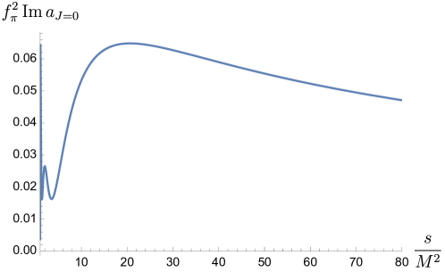
Figure 3: The spectral density at $J=0$ that saturates $\tilde{g}_{21}=0$, where the S-matrix is approximated by $N_{\rm max}=5$ polynomial.

4.1.2 Upper bounds on $g_{20}/g_{10}$ and $g_{21}/g_{10}$

To bootstrap the upper bounds, we simply flip the overall sign of $g_{20},g_{21}$ in the Lagrangians (86). The upper bound of $g_{20}$ in the unit of $g_{10}$ is also trivialized by the dual method

$${\frac{1}{3}}\big{(}-B_{1}^{(1)}+B_{1}^{(2)}+{\frac{1}{3}}B_{1}^{(3)}\big{)}\Big{|}_{p=0}\rightarrow g_{10}-g_{20}=\Big{\langle}{\frac{m^{2}-M^{2}}{m^{6}}}\Big{\rangle}\geq 0\rightarrow\tilde{g}_{2}=g_{20}/g_{10}M^{2}\leq 1\,.$$ (88)

The upper bound of $\tilde{g}_{2}^{\prime}=2g_{21}/g_{10}M^{2}$, although it is not straightforward, it can still be easily solved from the dual algorithm using SDPB Simmons-Duffin:2015qma . Using the crossing symmetric sum rules, we reproduced the result of Albert:2022oes

$$\tilde{g}_{2}^{\prime}\leq 3.25889135\,.$$ (89)

These two bounds are nontrivial from the primal side, since low spin sampling and low $N_{\rm max}$ would give us trash, which does not extrapolate well to an infinite dimensional SDP. For a more involved S-matrix bootstrap, which involves either linear unitarity or even complete unitarity, the strategy is to fix $N_{\rm max}$ and then increase $J_{\rm max}$ so that one can extrapolate the bounds to be valid for all $J$; subsequently, one should vary $N_{\rm max}$ and extrapolate the bounds to $N_{\rm max}=\infty$ Guerrieri:2021ivu ; Guerrieri:2022sod . However, for the positivity primal bootstrap, we find that we can simply fix $J_{\rm max}$ to a large value without doing the extrapolation. We choose $J_{\rm max}=60$, and we can see the nice convergence of bounds by varying $N_{\rm max}$ from $5$ to $25$, as shown in Fig 4. When $N_{\rm max}$ takes a small value, the approximation of the positivity EFT SDP is not good. However, we still expect the weak duality to be valid. This is precisely why we see that the primal upper bounds are always smaller than the dual upper bounds. Ultimately, we find that $N_{\rm max}=25$ is enough to conclude the strong duality, as the relative error of primal bounds from the dual bounds is roughly $\sim 1\%$.

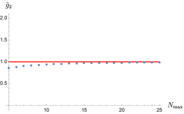
(a)

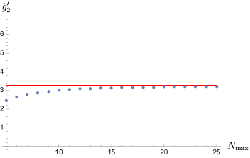
(b)

Figure 4: We determined the upper primal bounds of $\tilde{g}_{2}$ and $\tilde{g}_{2}^{\prime}$ by varying $N_{\rm max}$. These bounds converge quickly to the dual bounds, which are represented by red lines, approaching from below as guaranteed by the strong duality of SDP.

Now we can combine the dual and primal functionals to analyze the physical spectrum that saturates bounds. For primal side, we simply use the solutions from $N_{\rm max}=25$. The crucial point to understand is that since we are still far from the actual infinite-dimensional SDP, we cannot rely exclusively on either the dual functional or the primal solution to extract physical information. The strategy is as follows: initially, examine the dual functional. If the dual functional is precisely zero at a particular point, then we should trust the spectral density from the primal solution at that point, irrespective of its magnitude size. Conversely, if the dual functional is strictly positive and large, we would expect the corresponding primal “spectrum” to be small. Ideally, this primal spectrum should be vanishingly small. If it’s not, it should be small enough to be interpreted as a numerical artifact, and we should simply discard it. The most subtle situation arises when the dual functional is strictly positive and small enough to be approximated as zero. In this case, we should estimate the gap $Y_{J}(s){\rm Im}\,a_{J}(s)$ at that point. If the gap is sufficiently small, we can trust the primal spectrum; otherwise, we discard the data. However, this is also difficult to implement. It is worth noting that the dual functional is usually a polynomial of $M^{2}/s$, and is small for sufficiently high $s$ numerically. It is challenging to numerically detect that a small number is a zero or it is simply suppressed by $1/s$. This suggests that the EFT bootstrap does not have sharp implications in the deep UV, but a vague picture of the physics there can still be captured by the primal solutions: for large $s$, we believe that it is reasonable to trust the primal spectrum density, because we can always treat $Y_{\rho}(s)$ there as zero with small errors.

• $\tilde{g}_{2}=1$

From the dual functional (88), we see that $Y_{J}(s)$ can be zero only when $s=M^{2}$ and it is strictly positive for $s>M^{2}$, which is robust against adding more functionals. We indeed observe from the primal solution that there is a single peak around $s=M^{2}$ for $J=0$, see Fig 5; while ${\rm Im}\,a_{J}$ for $J\geq 1$ is vanishing. Besides, we also checked that the other Wilson coefficients at this point are $\tilde{g}_{2}^{\prime}=0$ and $\tilde{g}_{3}=g_{30}/g_{10}M^{4}\simeq 0.976\sim 1$. This analysis confirms that the UV theory with $\tilde{g}_{2}=1$ corresponds to a single scalar theory with mass $m=M$, as first pointed out by Albert:2022oes . The relevant scalar mode with $s^{0}$ Regge behaviour is

$$\mathcal{M}_{\rm scalar}(s,t)={\frac{M^{2}}{2f_{\pi}^{2}}}\big{(}{\frac{s}{M^{2}-s}}+{\frac{t}{M^{2}-t}}\big{)}\,.$$ (90)

A comparison of this scalar amplitudes with our numerical solution is illustrated in Fig 7(a). Nevertheless, it is important to note that the plot in Fig. 7(a) is drawn for the global region, which significantly suppresses the differences between the analytic and numerical amplitudes. The largest difference between amplitudes obtained by the two methods occurs at $|s|\rightarrow\infty$ and $t\rightarrow 0$, and is approximately $0.018$.

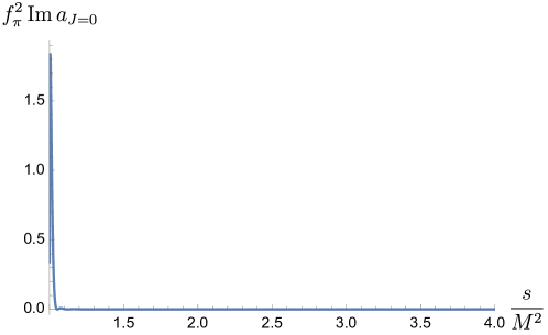
Figure 5: The spectral density at $J=0$ that saturates $\tilde{g}_{2}=0$. To generate this plot, we used a polynomial order in S-matrix of $N_{\rm max}=25$.

• $\tilde{g}_{2}^{\prime}\simeq 3.25889135$

The associated dual functional is complicated, but we can nevertheless easily observe that it is strictly positive for $J=0$ but it is zero for $J>0,s=M^{2}$. From the primal side, we indeed observe that ${\rm Im}\,a_{J=0}$, although not exactly zero, is parametrically small as of order $10^{-5}$; in addition, $J>0$ spectral density exhibits a sharp pump around $s=M^{2}$, which is, however, getting smaller and smaller for larger $J$. See Fig 6 for an illustration with $J=0,1,2,3$.

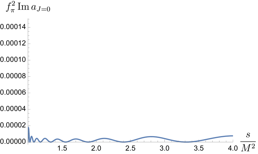
(a)

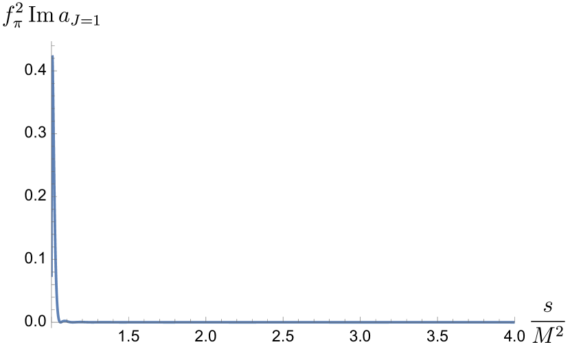
(b)

(c)

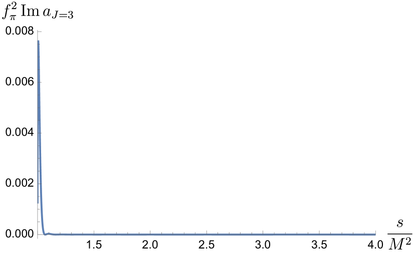
(d)

Figure 6: The spectral density from $J=0$ to $J=3$ is solved using $N_{\rm max}=25$ at $\tilde{g}_{2}^{\prime}\simeq 3.26$. The $J=0$ spectral density is nonphysical, as it is of the order $10^{-5}$, which is parametrically small compared to others. For higher $J$ values, we have smaller spectral densities, serving as a reminder of the low-spin dominance.

In addition, we find that this point gives $\tilde{g}_{2}\simeq 0.99\sim 1$ and $\tilde{g}_{3}\simeq 0.97\sim 1$. This analysis confirms the statement of Albert:2022oes that the UV theory with $\tilde{g}_{2}^{\prime}\simeq 3.26$ is a theory with $J\geq 1$ and $m=M$. However, it is important to note that our “numerical theory” is radically different from the $su$-model which also saturates $\tilde{g}_{2}^{\prime}\sim 3.26$ Albert:2022oes , because the $su$-model has Regge behaviour $s^{-1}$ while our ansatz grows like $s^{0}$. We can modify the $su$-model to describe a spin-$1$ theory with Regge behaviour $s^{0}$

$$\mathcal{M}_{su-{\rm mod}}(s,t)={\frac{M^{2}}{2(1-\log 2)f_{\pi}^{2}}}\Big{[}{\frac{s\,t}{(M^{2}-s)(M^{2}-t)}}+(1-\log 2)\Big{(}{\frac{s}{M^{2}-s}}+{\frac{t}{M^{2}-t}}\Big{)}\Big{]}\,.$$ (91)

We can then compare our numerical rule-in with this analytic rule-in in Fig. 7(b), where the maximal difference is around $0.017$

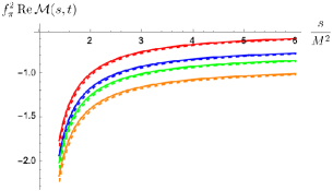
(a)

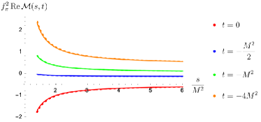
(b)

Figure 7: (a) The real part of the amplitudes $\mathcal{M}(s,t)$ with $\tilde{g}_{2}=1$ for several values of $t$. (b) The real part of the amplitudes $\mathcal{M}(s,t)$ with $\tilde{g}_{2}^{\prime}\simeq 3.26$ for several values of $t$. The solid lines are drawn from the analytic rule-in amplitudes (90) and (91) respectively, while the dashed lines are drawn from the primal solutions.

4.1.3 The Skyrme bound and a mysterious Regge trajectory

There is an interesting linear bound, giving rise to precisely the Skyrme model makhankov2012skyrme ; lenz1997lectures , as first noticed in Albert:2022oes . This bound involves $g_{21}$ and $g_{20}$, and we can formulate it as

$$\mathcal{L}=-g_{21}+\lambda(g_{20}-1)-\int_{M^{2}}^{\infty}ds\sum_{J}{\rm Im}\,a_{J}(s)Y_{J}(s)\,.$$ (92)

The bound is again trivial on the dual side, we have

$$B_{1}^{(1)}(p=0)\rightarrow 4g_{20}-2g_{21}=\Big{\langle}{\frac{2(1+(-1)^{J})}{s^{3}}}\Big{\rangle}\geq 0\rightarrow\tilde{g}_{2}^{\prime}\leq 4\tilde{g}_{2}\,.$$ (93)

According to the previous experience, $N_{\rm max}=25$ is good enough for us to perform a nice primal algorithm. We then find that the primal bound is

$$\tilde{g}_{2}^{\prime}\lesssim 3.939\,\tilde{g}_{2}\,,\quad\text{primal bound with $N_{\rm max}=25$}\,.$$ (94)

The error from the dual rigorous bound is around $1.54\%$.

Let’s now turn to analyze the physical spectrum of the Skyrme model. We observe that the simple dual functional $Y_{J}(s)$ can be zero only for odd $J$, which seems to suggest that we should discard all data with even spin in the primal solution. However, this conclusion is not robust against expanding the space of the dual functionals. When using $126$ functionals, we can find that the dual functional is small at $J=0,s=M^{2}$ (around $10^{-3}$), while it is strictly positive and not small close to $s=M^{2}$ for other $J$. With this in mind, we can examine the primal solution, and we find that the contributions from $J\neq 1$ are relatively smaller than those from $J=1$. This behaviour can be described as the vector meson dominance sakurai1960theory . Specifically, for $J=1$ we identify a sharp peak around $m=M$, which can be interpreted as a vector $\rho$ meson. There is also significant physics at higher energies: a continuum with a resonant bump around $m\approx 7.4M$ and a width of roughly $12.6M$, which might be a numerical artifact when compared to the $m=M$ peak. For other spins, we should only trust the behaviour at sufficiently high $s=m^{2}$, and we indeed observe dominate resonances at energies $m>7M$ with a relatively wide width. It is important to note that these resonances are stable upon increasing $N_{\rm max}$. Interestingly, if we consider $M$ as the mass of the $\rho$ meson, approximately $770{\rm MeV}$, then the mass of all those heavy resonances exceeds $4000{\rm MeV}$ and thus would contain, e.g., a bottom quark. See Fig 8 for an explicit illustration for $J=0,1,2,3$.

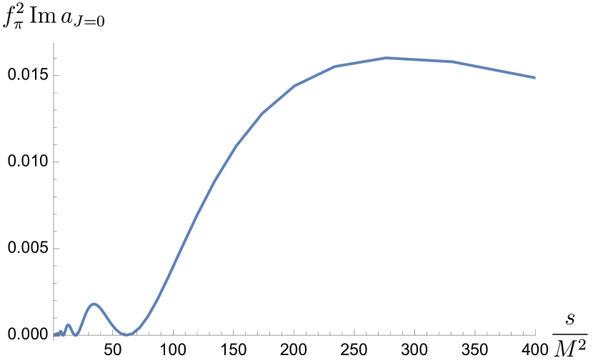
(a)

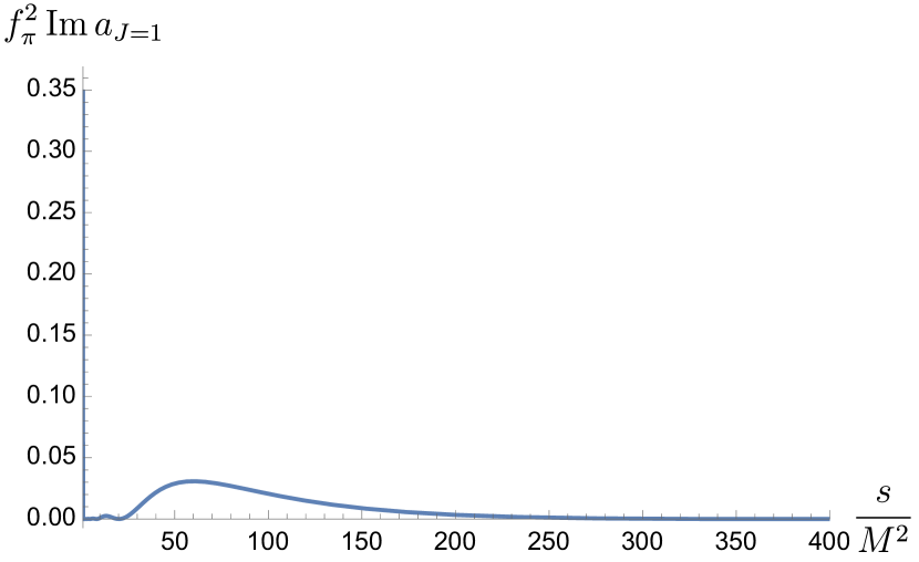
(b)

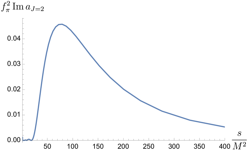
(c)

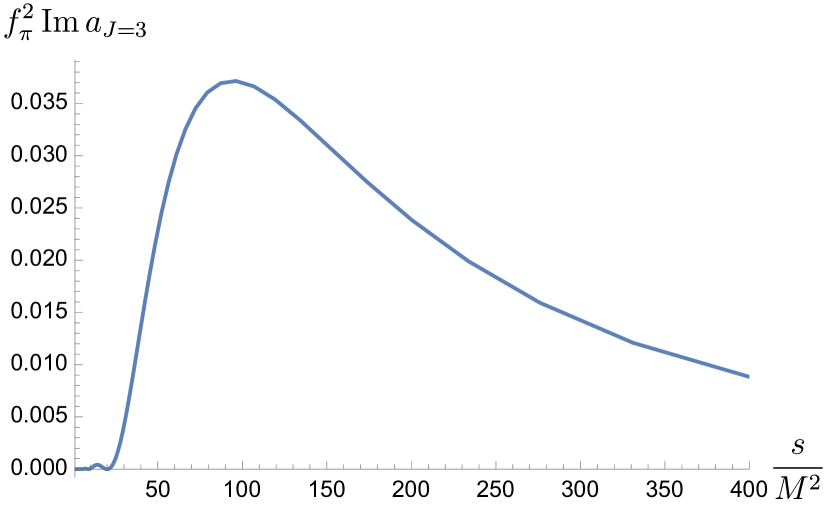
(d)

Figure 8: The spectral density for $J=0,1,2,3$ is solved using $N_{\rm max}=25$ on the Skryme line $\tilde{g}_{2}^{\prime}=4\tilde{g}_{2}$. The vector meson dominance is exhibited. For $J=1$, there is a vector $\rho$ meson with mass around $M$ and also other resonance around $7.4M$ that might be a numerical flaw; for other spins, there are dominated resonances at energy $s>50M^{2}$.

We can extend our primal analysis up to $J=10$ and find subsequent resonances. More surprisingly, these resonances can be organized as an approximately linear Regge trajectory, as shown in Fig 9. For higher $J$, we observe a significant deviation from the fitted Regge trajectory. This deviation is likely due to poor numerical shooting. Unfortunately, we have no clear explanation for this trajectory. It is possible that we should not take it from such high energy behaviour of primal solutions, and as inferred by Albert:2022oes , those resonances are actually pushed to infinity in the large-$N$ limit. Refining the numerics to better understand this Regge trajectory would be interesting in the future.

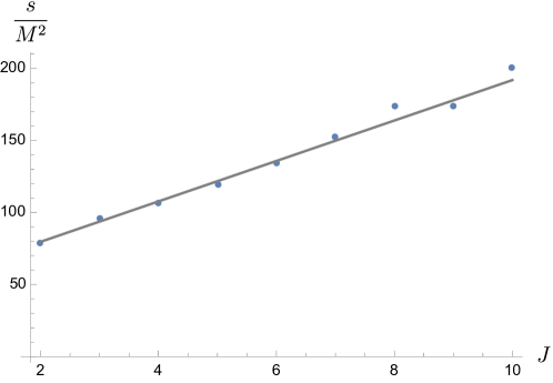
Figure 9: The Regge trajectory is read off from the primal solutions. This trajectory can be fitted as a linear line with minor errors.

Now we can compare the numerical amplitude to the model proposed in Albert:2022oes

$$\mathcal{M}_{{\rm spin}-1}^{(\rm UV)}={\frac{M^{2}}{2f_{\pi}^{2}}}{\frac{m_{\infty}^{2}}{M^{2}+3m_{\infty}^{2}}}\Big{(}{\frac{M^{2}+2t}{M^{2}-s}}{\frac{m_{\infty}^{2}}{m_{\infty}^{2}-t}}+{\frac{M^{2}+2s}{M^{2}-t}}{\frac{m_{\infty}^{2}}{m_{\infty}^{2}-t}}\Big{)}\,,$$ (95)

where it reduces to a single $\rho$ meson model in the limit $m_{\infty}\rightarrow\infty$. Our strategy of comparison is to first solve $m_{\infty}$ for requiring the Regge limit of this analytic model equals the numerical amplitude at fixed $t$ and then compare the amplitudes with other energy. We take $t=-1/10$ and find that $m_{\infty}\big{|}_{t=-1/10}\simeq 14.7M$, the comparison is displayed in Fig 10. We observe that although the extremely high energy limit is required to be the same, two amplitudes become clearly distinguishable at $s\sim 15M^{2}$. The difference at large $s$ but below $|s|\rightarrow\infty$ is anticipated, because (95) is just a toy model with a single resonance $m_{\infty}$ to adjust, while the primal solutions Fig 8 contain more than one resonance, organized as a Regge trajectory Fig 9. We can also evaluate the Wilson coefficients that saturate the Skyrme bound from our primal solution, $\tilde{g}_{2}\simeq 0.364,\tilde{g}_{2}^{\prime}\simeq 1.434,\tilde{g}_{3}\simeq 0.349$, which are close to what (95) predicts $(1/3,4/3,1/3)$.

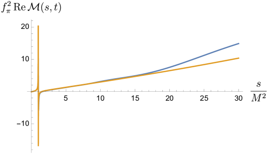
Figure 10: The comparison between the numerical amplitude from the primal solution with $N_{\rm max}=25$ (blue) and the UV model (95) with $m_{\infty}\simeq 14.7M$ (yellow).

4.2 Exclusion plots

4.2.1 $\mathcal{O}(p^{4})$

So far, we have only dealt with simple linear bounds. The power of the EFT bootstrap lies in its ability to search for allowed spaces that involve multiple Wilson coefficients. These represent nonlinear bounds, implying that the boundary is not a linear function. Let’s focus on the space spanned by $\tilde{g}_{2}^{\prime}$ and $\tilde{g}_{2}$ and reproduce the exclusion plot made using dual methods in Albert:2022oes .

Our strategy is to search in different directions in the $\tilde{g}_{2}^{\prime}-\tilde{g}_{2}$ plane. The corresponding Lagrangian is

$$\mathcal{L}_{p^{4}}=\big{(}\cos(2\pi c)g_{20}+\sin(2\pi c)g_{21}\big{)}+\lambda(g_{10}-1)-\int_{M^{2}}^{\infty}ds\sum_{J}{\rm Im}\,a_{J}(s)Y_{J}(s)\,,$$ (96)

where $c\in[0,1)$. On the dual side, this corresponds to fixing the objective and varying the normalization condition; while on the primal side, this precisely means fixing the normalization to $g_{10}=1$ and bounding different linear combinations of $g_{20}$ and $g_{21}$. There is another approach, different from these angle-searching methods. In this approach, one can fix a particular value of one parameter, for example, $g_{20}/g_{10}$, and search for the upper and lower bounds of another parameter $g_{21}/g_{10}$ Caron-Huot:2020cmc . While this method is typically as efficient as the previous one on the dual side, it complicates the search on the primal side. This is because it fixes two parameters, $g_{20}$ and $g_{10}$, making the positive matrices degenerate. Consequently, an additional transformation is needed to generate a valid positivity input. Nevertheless, near the corner, it is aways better to adopt the “fixing-parameter” method rather than the “angle-searching”. We leave the details of “fixing-parameter” methods in appendix C.

By sampling a sufficient number of $c$ values (roughly $100$ points) and few “fixing-parameter” points near the corner, we can make a sufficiently nice exclusion plot using both dual and primal methods (where we choose $N_{\rm max}=25$). The plot is displayed in Fig 11, where the dashed black boundary is drawn using the dual method, coinciding with the findings in Albert:2022oes ; on the other hand, the solid boundary is derived from the primal method. We find that the primal bounds efficiently converge to the dual bounds. To generate the dual bounds, we use $126$ functionals that are constructed from the crossing symmetric sum rules $B_{1},B_{3},B_{5}$.

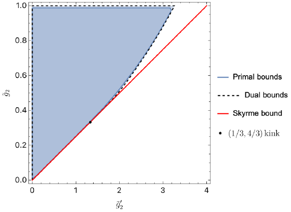
Figure 11: The exclusion plot involves $\tilde{g}_{2}$ and $\tilde{g}_{2}^{\prime}$, and compares the primal bounds to the dual bounds. The red line represents the linear Skyrme bound and the black dot is the position of $(1/3,4/3)$ kink.

We observe from Fig 11 that the Skyrme line represents only a small segment of the entire boundary. The point where the bounds begin to deviate from the Skyrme model is referred to as a “kink” in Albert:2022oes . Nontrivial physics is anticipated at this kink El-Showk:2012cjh ; Albert:2022oes . Further studies suggest that the kink is located at the point $(\tilde{g}_{2},\tilde{g}_{2}^{\prime})=(1/3,4/3)$ Fernandez:2022kzi , which is ruled-in by the analytic model (95) with $m_{\infty}\rightarrow\infty$. We present several points on the boundary in Fig 11, retaining three digits after the decimal, as shown in Table 1. We note that around $\tilde{g}_{2}\simeq 0.26$, the value of $\tilde{g}_{2}^{\prime}$ is already slightly smaller than what the Skyrme bound predicts, which is, however, likely to be numerical error. Therefore, using our dual numerical results does not provide sensible way to clearly pinpoint the position of the kink.

$\tilde{g}_{2}$	$\tilde{g}_{2}^{\prime}$
$0.001$	$0.004$
$0.005$	$0.020$
$0.020$	$0.080$
$0.120$	$0.480$
$0.250$	$1.000$
$0.260$	$1.039$
$0.333$	$1.332$
$0.390$	$1.577$

Table 1: Few boundary points with small $\tilde{g}_{2}$, obtained using the dual methods.

4.2.2 $\mathcal{O}(p^{6})$

For $\mathcal{O}(p^{6})$, we consider a similar Lagrangian but for $g_{30},g_{31}$

$$\mathcal{L}_{p^{6}}=\big{(}\cos(2\pi c)g_{30}+\sin(2\pi c)g_{31}\big{)}+\lambda(g_{10}-1)-\int_{M^{2}}^{\infty}ds\sum_{J}{\rm Im}\,a_{J}(s)Y_{J}(s)\,,$$ (97)

Following the same strategy as noted previously, we can create the exclusion plot for $\tilde{g}_{3}=g_{30}M^{4}/g_{10}$ and $\tilde{g}_{3}^{\prime}=g_{31}M^{4}/g_{10}$. There is a good convergence between the primal and dual methods, as seen in Fig 12.

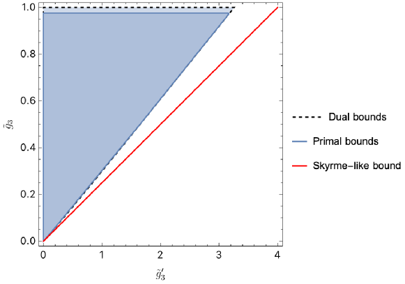
Figure 12: The exclusion plot involves $\tilde{g}_{3}$ and $\tilde{g}_{3}^{\prime}$, with comparison of the primal bounds to the dual bounds. The red line represents the linear Skyrme-like bound $\tilde{g}_{3}^{\prime}\leq 4\tilde{g}_{3}$.

Some comments are in order. Interestingly, we find that the linear upper bound of $\tilde{g}_{3}$ and $\tilde{g}_{3}^{\prime}$ is the same as in $\tilde{g}_{2}$ and $\tilde{g}_{2}^{\prime}$. This is because that the corner can still be analytically ruled in by (91). and we also have the Skyrme-like linear bound $\tilde{g}_{3}^{\prime}\leq 4\tilde{g}_{3}$. However, it is obvious from Fig 12 that the whole allowed region is much smaller than the region enclosed by the linear bounds, even though there is no clear kink. In this case, the nonlinearity largely shrinks the allowed space of EFT. The same phenomenon was also observed in gravitational EFT Bern:2021ppb ; Caron-Huot:2022ugt ; Chiang:2022jep .

4.3 Is the positivity primal bootstrap sensitive to the Regge behaviour?

In this subsection, we aim to address the question of whether the Regge behaviour in the primal ansatz affects the primal bounds. The answer should be “No” for the positivity bootstrap, as long as the Regge behaviour is below $k_{0}=1$ ensuring that our dual set-up remains valid. This is confirmed by the duality between the dual and primal methods: the dual bounds are only sensitive to $k_{0}$, which provides all sum rules. Therefore, the primal bounds should not depend on the specifics of the Regge behaviour of the amplitudes, as long as their growth rate is below $k_{0}$. However, if the Regge behaviour of the primal ansatz reaches $k_{0}$ or exceeds it, it cannot measure and provide bounds on the Wilson coefficients with Regge spin $k_{0}$.

Our strategy is to choose $\mathcal{R}(s,t)$ in the ansatz (86) as

$$\mathcal{R}(s,t)=\big{(}(1+\sqrt{1-s})(1+\sqrt{1-t})\big{)}^{2J^{0}}\,.$$ (98)

For $J^{0}=0$, we recover the case that we have been studying. In general, this factor modifies the dictionary that relates the ansatz parameters $\alpha_{ab}$ to the low-energy Wilson coefficients, but it preserves the analyticity and grows as $s^{J^{0}}$ in the Regge limit. We will study the primal upper bound of $\tilde{g}_{2}^{\prime}$, which can be measured by $B_{1}$ sum rules and is sufficiently nontrivial. We will vary $J^{0}$ by taking several values: $J^{0}=(0,0.5,0.75,1,1.1)$ and observe how the primal bounds change accordingly. This exploration is displayed in Fig 13 below. In Fig 13, we present only the results for $J^{0}=(0,0.5,0.75)$, and it’s clear that they all converge to the dual rigorous bound at sufficiently large $N_{\rm max}$. For $J^{0}=1,1.1$, as expected, we do not obtain any bounds.

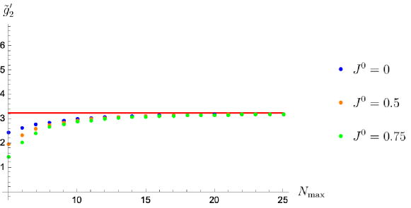
Figure 13: The primal upper bound of $\tilde{g}_{2}^{\prime}$ from the primal ansatz with different Regge behaviour $s^{J^{0}}$.

4.4 An ad hoc: primally confirming the large-$N$ assumption

So far, we have been considering the constraints of the large-$N$ $\chi$PT, as suggested in Albert:2022oes . As previously noted, we assume the large-$N$ limit from IR to UV; therefore, the positivity bootstrap is sufficient and strongly constraining. In this way, we can bound the Wilson coefficients in terms of $g_{10}=1/(2f_{\pi}^{2})\sim 1/N$. Nevertheless, it is essential to question whether this assumption is justified from a low-energy point of view. In other words, do the large-$N$ bounds fall into the allowed regime of a more complete unitary region like linear unitarity?

This question may seem trivial, since there is no doubt that the spectral density scaling as $1/N$ falls into the linear unitarity ${\rm Im}\,a_{J}\sim 1/N\ll 2$. Indeed, this simple argument trivializes the linear bound: the large-$N$ limit yields bounds that scale in $g_{10}$, i.e., $g\leq\mathcal{O}(1)g_{10}/M^{{\rm dim}-2}$, which are significantly stronger than the bounds provided by linear unitarity, $g\leq\mathcal{O}(1)/M^{\rm dim}$, because $g_{10}\ll 1/M^{2}$. However, it is important to emphasize that this straightforward argument and power counting do not obviously work for nonlinear bounds. The dimensional analysis can only infer that the large-$N$ exclusion plot resides in the near-zero corner in the linear unitarity plot, however, its boundary may bend outside of the region of the linear unitarity exclusion plot. This concern arises due to results of Chiang:2022ltp ; Chen:2022nym , where it turns out that the boundary of the linear unitarity bounds is more curved and is sandwiched between the linear bounds.

Our strategy to justify the large-$N$ bound involves using the linear unitarity bootstrap for pion amplitudes, whose structures remain constrained by the large-$N$ limit. We employ only the primal method. For the dual method that incorporates the upper bound of unitarity, see Caron-Huot:2020cmc ; Chiang:2022ltp ; Chiang:2022jep ; Chen:2023bhu . For a recent systematic numerical algorithm on the dual side, refer to Chen:2023bhu . For simplicity, we take $N_{f}=2$, then (72) indicates that the unitarity constraints are

$$0\leq{\rm Im}\,a_{{\rm even}\,J}(s)\leq{\frac{1}{3}}\,,\quad 0\leq{\rm Im}\,a_{{\rm odd}\,J}(s)\leq{\frac{1}{2}}\,.$$ (99)

Follow appendix A, we then consider the following SDP Lagrangian

$$\mathcal{L}_{\rm up} =\big{(}\cos(2\pi c)g_{20}+\sin(2\pi c)g_{21}\big{)}-\int_{M^{2}}^{\infty}ds\sum_{J}{\rm Im}\,a_{J}(s)Y_{J}(s)$$

$$-\int_{M^{2}}^{\infty}ds\sum_{{\rm even}\,J}\big{(}{\frac{1}{2}}-{\rm Im}\,a_{J}(s)\big{)}\tilde{Y}_{J}(s)-\int_{M^{2}}^{\infty}ds\sum_{{\rm odd}\,J}\big{(}{\frac{1}{3}}-{\rm Im}\,a_{J}(s)\big{)}\tilde{Y}_{J}(s)\,.$$ (100)

In this case, we physically “normalize” the free theory part $S=1+iT$. Although in this case, the numerical convergence is more slow, we find that $N_{\rm max}=25$ and $J_{\rm max}=60$ still suffice for our purpose. By searching different values of $c$, we found Fig 14, where we define $\widehat{g}_{2}^{\prime}=2g_{21}M^{4}$ and $\widehat{g}_{2}=g_{20}M^{4}$.

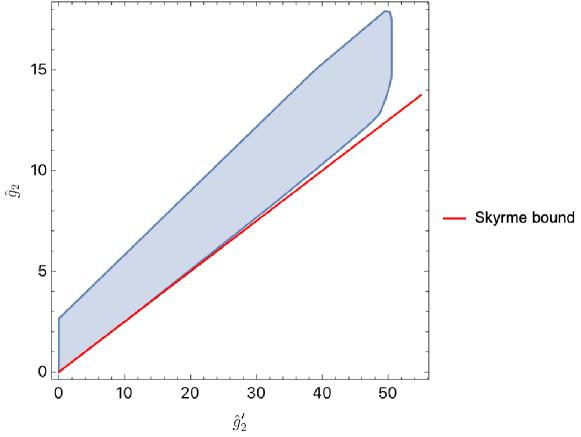
Figure 14: The exclusion plot for $\widehat{g}_{2}$ and $\widehat{g}_{2}^{\prime}$ from the primal linear unitarity bootstrap.The red line still represents the linear Skyrme bound $\widehat{g}_{2}^{\prime}\leq 4\widehat{g}_{2}$.

From Fig 14, we can confirm that the linear bounds are indeed consistent with the large-$N$ bounds as long as $N\sim\mathcal{O}(10)$. Nevertheless, we do observe dangerous regions. The first dangerous region is around $\widehat{g}_{2}\sim 2.7$, where there is a sharp kink, and the boundary shrinks away from the vertical line. In contrast, the large-$N$ bounds in Fig 11 do not exhibit this shrinking. To resolve this danger, we need to require

$$f_{\pi}^{2}\geq 0.19M^{2}\,.$$ (101)

The second danger is the Skyrme line. In this plot, the lower boundary behaves similarly to the large-$N$ plot: it first coincides with the Skyrme bound and then bends inward. Therefore, the position of the “Skyrme kink” in Fig 14 must be larger than the one in the large-$N$ case. Fortunately, the kink in Fig 11 is around $\widehat{g}_{2}^{\prime}\sim 11.6$, for which the condition (101) easily resolves the danger. Since (101) can be easily satisfied in the large-$N$ limit where $f_{\pi}^{2}\sim N\rightarrow\infty$, we thus confirm that assuming the large-$N$ limit at low energy is valid without paradox. Besides, we emphasize that this exercise also shows that the unitarity can be used to bound the decay constant in terms of the EFT scale $M$. Indeed, we can set an EFT bootstrap to directly constrain the decay constant $f_{\pi}$ which deserves further exploration for finite $N$ $\chi$PT

5 Constrain holographic QCD models

Large-$N$ QCD enjoys holographic descriptions, which utilize the dual gravity theory to capture the salient properties of QCD, such as hadrons, in the strong coupling limit. One famous example of these models is known as the Witten-Sakai-Sugimoto model Witten:1998zw ; Sakai:2004cn ; Sakai:2005yt , which can be constructed from string theory. Such models can also be built from low-energy EFTs of gauge fields with gravitational couplings Son:2003et ; Kim:2009qs ; Erlich:2005qh ; DaRold:2005mxj ; Hirn:2005nr ; Panico:2007qd ; Colangelo:2012ipa , where the fits to the experimental data of hadrons, glueballs, and so on have been extensively studied (see e.g., Erdmenger:2007cm ; Pahlavani:2014dma for brief reviews). Typically, at low energy, the holographic models can also give rise to the $\chi$PT Lagrangian with Wilson coefficients mapping to parameters on the gravity side Sakai:2004cn ; Sakai:2005yt ; Kim:2009qs ; Erlich:2005qh ; DaRold:2005mxj ; Hirn:2005nr ; Panico:2007qd ; Colangelo:2012ipa . Therefore, we expect that the bounds on large-$N$ $\chi$PT can be translated into constraints on those holographic QCD models, carving out the allowed space of EFTs for gauge theories that can be consistently UV completed with gravity.

However, to our knowledge, all holographic QCD models so far only include ${\rm Tr}\,F^{2}$ term when deriving the $\chi$PT, giving rise to the Skryme model at order $\mathcal{O}(p^{4})$. The essential reason is that higher derivative terms are relatively small, like suppressed by the string scale Sakai:2004cn ; Sakai:2005yt . Therefore, one can always adjust the fundamental parameters so that the Wilson coefficients live on the boundary of the exclusion plot 11 below the kink. Nevertheless, although the higher derivative terms only give small corrections, these small corrections may still deform the Wilson coefficients outside of the allowed region in Fig 11. In this section, we will show that higher derivative terms ${\rm Tr}\,F^{3}$ and ${\rm Tr}\,F^{4}$ cause the low-energy theory deviate from the Skyrme model. Therefore, requiring the consistency with Fig 11 puts constraints on the higher derivative couplings.

5.1 Chiral Lagrangian from holographic QCD

5.1.1 Bulk theory and the power counting

We now move to derive the chiral Lagrangian from $5D$ EFT of ${\rm SU}_{\rm L}(N_{f})\times{\rm SU}_{\rm R}(N_{f})$ gauge fields. We consider the following effective action with the background field $\overline{g}$

$$S_{\rm eff}=\sum_{i={\rm L},{\rm R}}{\frac{1}{g_{\rm YM}^{2}}}\int d^{5}x\sqrt{-\overline{g}}\,\varphi(x)\Big{(}-{\frac{1}{2}}{\rm Tr}\,F_{i}^{2}+{\frac{ig_{H}}{3}}{\rm Tr}\,F_{i}^{(3)}+{\frac{\alpha_{1}}{4}}{\rm Tr}\,F_{i}^{4}+{\frac{\alpha_{2}}{4}}{\rm Tr}\,F_{i}^{(4)}\Big{)}\,,$$ (102)

where

$${\rm Tr}\,F^{2}={\rm Tr}\Big{(}F_{AB}F^{AB}\Big{)}\,,\quad{\rm Tr}\,F^{(3)}={\rm Tr}\Big{(}F_{A}\,^{B}[F_{B}\,^{C},F_{C}\,^{A}]\Big{)}\,,$$

$${\rm Tr}\,F^{4}={\rm Tr}\Big{(}F_{AB}F^{AB}F_{CD}F^{CD}\Big{)}\,,\quad{\rm Tr}\,F^{(4)}={\rm Tr}\Big{(}F_{A}\,^{B}F_{B}\,^{C}F_{C}\,^{D}F_{D}\,^{A}\Big{)}\,.$$ (103)

All $A,B,\cdots$ refer to the five dimensional indices, and all indices so far are contracted by the background field $\overline{g}_{AB}$ and a background dilaton $\varphi$

$$ds^{2}=\overline{g}_{AB}dX^{A}dX^{B}=b(z)^{2}dz^{2}+a(z)^{2}\eta_{\mu\nu}x^{\mu}x^{\nu}\,,\quad z\in[z_{\rm UV},z_{\rm IR}]\,,$$ (104)

where we put an UV Randall-Sundrum (RS) bane Randall:1999ee ; Randall:1999vf at $z_{\rm UV}$ and an IR RS brane at $z_{\rm IR}$. For Anti de-Sitter (AdS) space, the UV brane is served as the boundary of AdS. Nevertheless, throughout this subsection, we consider $a(z),b(z)$ and $\varphi$ to be arbitrary. Their precise forms satisfy the equations of motion for both the gravity sector and the matter sectors (such as dilaton associated with $\varphi$ Sakai:2004cn ; Sakai:2005yt ; Karch:2006pv ). However, we treat the flavour gauge fields as probes Sakai:2004cn ; Sakai:2005yt . Appropriate boundary conditions are imposed on both the UV brane at $z_{\rm UV}\rightarrow 0$ and the IR brane $z_{\rm IR}$ to obtain the background solution (104). We ignore fluctuations from the graviton and other matters, as they are irrelevant for our purposes.

How should we think about the EFT power counting of (102) without a top-down picture like string theory? The bulk gauge fields are expected to correspond to conserved currents in QCD. Hence, we then have $J_{L}^{\mu a}$ and $J_{R}^{\mu a}$, which can be constructed by quark bilinear operators $J^{\mu a}=q\gamma^{\mu}T^{a}\overline{q}$; their conservation precisely reflects the global chiral symmetry. From large-$N$ counting, we know that we usually scale such quark bilinear operators by $1/\sqrt{N}$ to normalize the two-point function t1993planar ; this corresponds to scaling $A$ by $g_{\rm YM}$ to normalize the kinematic term, suggesting $g_{\rm YM}\sim 1/\sqrt{N}$ in (102). Moreover, the Wilson coefficients $g_{H},\alpha_{i}$ should be suppressed by some EFT cut-off $\Lambda$, which could be the mass of higher spin particles or the string states (it’s important to distinguish it from the $\chi$PT EFT cut-off $M$ for the moment). However, due to the presence of $g_{\rm YM}$, there are different possible consistent schemes of power counting for $g_{H}$ and $\alpha_{i}$, as long as their sizes don’t grow beyond $\langle F\rangle^{\#}$. For instance, we can have $g_{H}\sim 1/\Lambda^{2},\alpha_{i}\sim 1/\Lambda^{4}$; or we can have $g_{H}\sim g_{\rm YM}^{2}/\Lambda,\alpha_{i}\sim g_{\rm YM}^{2}/\Lambda^{2}$, both of which are then suppressed by the large-$N$ limit. The idea is then to use the EFT constraints to decide the correct size of those Wilson coefficients. It’s important to note that we actually ignore some double trace terms like $\big{(}{\rm Tr}\,F^{2}\big{)}^{2}$, because ${\rm Tr}$ maps to the trace in $\chi$PT, and coefficients of double-trace operators in large-$N$ $\chi$PT are $1/N$ suppressed, for general $N_{f}$. Therefore, we conclude for $N_{f}>3$, without doing anything, that the Wilson coefficient of $1/g_{\rm YM}^{2}\big{(}{\rm Tr}\,F^{2}\big{)}^{2}$ must scale at least as $g_{\rm YM}^{2}/\Lambda^{2}$! Indeed, in the Witten-Sakai-Sugimoto model from the $D_{4}$-$D_{8}$-$\overline{D}_{8}$ intersection, the effective action is the dilaton-Born-Infeld (DBI) action Sakai:2004cn , which still has only a single trace when generalized to the non-Abelian case Hagiwara:1981my .

5.1.2 Routine to obtain the chiral Lagrangian

We follow the strategy of Panico:2007qd that uses the IR boundary condition to break the chiral symmetry

$$A_{L\mu}(z_{\rm IR})-A_{R\mu}(z_{\rm IR})=0\,,\quad F_{L\mu z}(z_{\rm IR})+F_{R\mu z}(z_{\rm IR})=0\,.$$ (105)

This implies that the chiral symmetry breaks to its vector subgroup at IR. For convenience, we regroup the gauge group by its vector component and axial component

$$\mathcal{V}_{\mu}={\frac{1}{2}}(A_{L\mu}+A_{R\mu})\,,\quad\mathcal{A}_{\mu}={\frac{1}{2}}(A_{L\mu}-A_{R\mu})\,.$$ (106)

It turns out that one can define a Wilson line stretch from the IR point into the bulk

$$U=P\Big{\{}e^{i\int_{z_{\rm IR}}^{z}dzA_{Lz}}e^{-i\int_{z_{\rm IR}}^{z}dzA_{Rz}}\Big{\}}\,,$$ (107)

which has the property of the pion field under the gauge transformation $U\rightarrow g_{R}Ug_{L}^{-1}$, and thus it corresponds to $U$ in $\chi$PT at the UV point. For simplicity, we choose the gauge $A_{Rz}\equiv 0$, and use $U$ to gauge away $A_{Lz}$ using the gauge fixing prescription of Sakai:2004cn ; Hirn:2005nr ; Panico:2007qd . This procedure allows us to define the following boundary condition

$${\rm IR}:\,\quad\partial_{z}\mathcal{V}_{\mu}(x,z_{\rm IR})=0\,,\quad\mathcal{A}_{\mu}(x,z_{\rm IR})=0\,,$$

$${\rm UV}:\,,\quad\mathcal{V}_{\mu}(x,z_{\rm UV})=\mathcal{A}_{\mu}(x,z_{\rm UV})={\frac{i}{2}}U\partial_{\mu}U^{\dagger}\,.$$ (108)

To obtain an effective action, one can solve the bulk gauge fields with respect to these boundary conditions, and then substitute the solutions back to have the on-shell action. For simplicity, in this paper, we only focus on those terms up to $\mathcal{O}(p^{4})$, therefore we can simply solve the equation of motion at leading order Panico:2007qd

$$\mathcal{V}_{\mu}(x,z)=\mathcal{V}_{\mu}(x,z_{\rm IR})+\cdots\,,\quad\mathcal{A}_{\mu}(x,z)=f_{A}(z)\mathcal{A}_{\mu}(x,z_{\rm IR})+\cdots\,,$$ (109)

where $\cdots$ refer to those terms contributing to higher orders like $\mathcal{O}(p^{6})$, and one has

$$f_{A}(z)=c_{A}\int_{z}^{z_{\rm IR}}d\xi{\frac{b(\xi)}{a(\xi)^{2}\varphi(\xi)}}\,,\quad f_{A}(z_{\rm UV})=1\,.$$ (110)

It is then straightforward to obtain the chiral Lagrangian (61), where the pion decay constant $f_{\pi}$ and other Wilson coefficients are given by

$$l_{1}={\frac{1}{16g_{\rm YM}^{2}}}\int_{z_{\rm UV}}^{z_{\rm IR}}dz\frac{\varphi(z)\left(-4b(z)^{2}g_{H}\left(f_{A}(z){}^{2}-1\right)f_{A}^{\prime}(z){}^{2}-2b(z)^{4}\left(f_{A}(z){}^{2}-1\right){}^{2}+\left(2\alpha_{1}+\alpha_{2}\right)f_{A}^{\prime}(z){}^{4}\right)}{b(z)^{3}}\,,$$

$$l_{2}={\frac{1}{8g_{\rm YM}^{2}}}\int_{z_{\rm UV}}^{z_{\rm IR}}dz\frac{\varphi(z)\left(f_{A}(z){}^{2}-1\right)\left(b(z)^{2}\left(f_{A}(z){}^{2}-1\right)+2g_{H}f_{A}^{\prime}(z){}^{2}\right)}{b(z)}\,,$$

$$f_{\pi}^{2}={\frac{2}{g_{\rm YM}^{2}}}\int_{z_{\rm UV}}^{z_{\rm IR}}dz\,{\frac{a(z)\varphi(z)f_{A}^{\prime}(z)^{2}}{b(z)}}\,.$$ (111)

5.2 Bounds for different models

5.2.1 Witten-Sakai-Sugimoto model is healthy

The Witten-Sakai-Sugimoto model, constructed from the $D_{4}$-$D_{8}$-$\overline{D}_{8}$ brane configuration in type IIA string theory, is considered a top-down model and is expected to be robust. Therefore, before imposing constraints on more general bottom-up models like (102), we aim to verify the health of the Witten-Sakai-Sugimoto model from a low-energy perspective.

The essential idea is to start with the $D_{8}$ brane embedded in the $D_{4}$ configuration

$$ds_{D_{8}}^{2}={\frac{2}{3(1+z^{2})^{{\frac{5}{6}}}}}\big{(}dz^{2}+(1+z^{2})^{{\frac{4}{3}}}\eta_{\mu\nu}dx^{\mu}dx^{\nu}+{\frac{9}{4}}(1+z^{2})d\Omega_{4}^{2}\big{)}\,,\quad z\in(-\infty,\infty)\,,$$

$$e^{\phi}=\sqrt{\frac{2}{3}}\sqrt[4]{z^{2}+1}g_{s}\,,\quad F_{4}=dC_{3}={\frac{2\pi N}{{\rm Vol}_{4}}}\epsilon_{4}\,,$$ (112)

on which we have the DBI action

$$S=-{\frac{1}{(2\pi)^{8}\ell_{s}^{9}}}\int d^{9}x\sqrt{-g}\,e^{-\phi}\Big{(}-{\rm Tr}\big{\{}{\rm det}\big{[}g_{MN}-2i\pi\alpha^{\prime}F_{MN}\big{]}\big{\}}\Big{)}^{{\frac{1}{2}}}\,.$$ (113)

Since we have the complete picture from the string theory, we can easily keep track of the power counting (where we keep the leading KK tower mass to be $M_{KK}=1$ for simplicity) Sakai:2004cn ; Sakai:2005yt

$$\alpha^{\prime}=\ell_{s}^{2}={\frac{9}{2\lambda}}\,,\quad g_{s}={\frac{\lambda^{{\frac{3}{2}}}}{3\sqrt{2}N\pi}}\,,\quad\lambda=g_{{\rm YM},c}^{2}N\,.$$ (114)

$\lambda$ is the ’t Hooft coupling, where $g_{{\rm YM},c}$ is the Yang-Mills coupling for the colour sector on $D_{4}$ brane. The weakly-coupled supergravity regime is only valid for $\lambda\rightarrow\infty,N\rightarrow\infty$.

To map this model to our bottom-up EFT (102), we cut the brane in half for $z\in(-\infty,0)$ and introduce an additional gauge field to compensate for the contribution from the other half, where $z_{\rm UV}=-\infty$ and $z_{\rm IR}=0$. We find

$$\varphi=\frac{9\sqrt{3}(1+z^{2})^{{\frac{1}{12}}}}{4\sqrt{2}}\,,\quad a(z)=\sqrt{\frac{2}{3}}(1+z^{2})^{{\frac{1}{4}}}\,,\quad b(z)=\frac{\sqrt{\frac{2}{3}}}{\left(1+z^{2}\right)^{5/12}}\,,\quad g_{\rm YM}^{2}=\frac{486\pi^{3}}{\lambda N}\,.$$ (115)

Besides, expanding in $\alpha^{\prime}$ yields Hagiwara:1981my

$$g_{H}=0\,,\quad\alpha_{1}=-\pi^{2}(\alpha^{\prime})^{2}\,,\quad\alpha_{2}=4\pi^{2}(\alpha^{\prime})^{2}\,.$$ (116)

Using the dictionary (111), we find

$$f_{\pi}^{2}={\frac{\lambda N}{54\pi^{4}}}\,,\quad l_{1}=-f_{\pi}^{2}\big{(}0.122985-{\frac{4.62298}{\lambda^{2}}}\big{)}\,,\quad l_{2}=0.122985f_{\pi}^{2}\,.$$ (117)

At the leading order when $\lambda\rightarrow\infty$, we reproduce the results of Sakai:2004cn ; Sakai:2005yt . We can immediately see that the string correction causes the Wilson coefficients to deviate from the Skyrme model. To compare with the large-$N$ $\chi$PT bound, we should examine $\tilde{g}_{2}^{\prime}$ and $\tilde{g}_{2}$

$$\tilde{g}_{2}=0.491942{\frac{M^{2}}{M_{KK}^{2}}}+{\frac{18.4919M^{2}}{\lambda^{2}M_{KK}^{2}}}\,,\quad\tilde{g}_{2}^{\prime}=1.96777{\frac{M^{2}}{M_{KK}^{2}}}\,.$$ (118)

At leading order, this is constrained to be below the kink for $M^{2}\leq 0.68M_{KK}^{2}$. Indeed, the KK spectroscopy analysis suggests that the $\rho$ mass is $M_{\rho}^{2}=0.67M_{KK}^{2}$! The string correction then pushes $\tilde{g}_{2}^{\prime}$ and $\tilde{g}_{2}$ upwards from the boundary, ensuring they still fall within the allowed region of Fig 11. We thus conclude that, even when including the leading string correction, we do not identify problems with the Witten-Sakai-Sugimoto model.

5.2.2 Flat and AdS hard wall models

Now we move to constrain two known holographic QCD models with $\varphi=1$. We focus on two models, one is constructed in the flat space as RS scenario Son:2003et , another is the hard wall model Hirn:2005nr constructed in AdS. They are both clearly explained in Hirn:2005nr . We believe that our discussions can be generalized to other holographic QCD models (with possible modifications on how the chiral symmetry is breaking), like the soft wall models, where the dilaton $\varphi$ is nontrivially turned out Karch:2006pv ; Ballon-Bayona:2020qpq ; Ballon-Bayona:2021ibm ; Afonin:2022qby .

• Flat space scenario Son:2003et

  For this model, we consider

  $$a(z)=b(z)=\varphi(z)=1\,,\quad z\in(0,z_{\rm IR}]\,,$$ (119)

  where we fix the UV brane to be $z_{\rm UV}=0$, and $z_{\rm IR}\sim 1/\Lambda_{\rm QCD}$. We have

  $$f_{\pi}^{2}={\frac{2}{g_{\rm YM}^{2}z_{\rm IR}}}\,,\quad l_{1}=\frac{15\alpha+40g_{H}z_{\text{IR}}^{2}-16z_{\text{IR}}^{4}}{240g_{\text{YM}}^{2}z_{\text{IR}}^{3}}\,,\quad l_{2}=\frac{2z_{\text{IR}}^{2}-5g_{H}}{30g_{\text{YM}}^{2}z_{\text{IR}}}\,,$$

  $$\tilde{g}_{2}=\frac{\pi^{2}\left(15\alpha-40g_{H}z_{\text{IR}}^{2}+16z_{\text{IR}}^{4}\right)}{480z_{\text{IR}}^{4}}\,,\quad\tilde{g}_{2}^{\prime}=\frac{1}{15}\pi^{2}\left(2-\frac{5g_{H}}{z_{\text{IR}}^{2}}\right)\,,$$ (120)

  where we have used $M^{2}\sim M_{\rho}^{2}=\pi^{2}/(4z_{\rm IR}^{2})$ Son:2003et . Besides, we denote $2\alpha_{1}+\alpha_{2}=\alpha$, which is the unique combination appears. We can easily observe some simple linear bounds

  $$\tilde{g}_{2}^{\prime}>0\rightarrow\tilde{g}_{H}={\frac{g_{H}}{z_{\rm IR}^{2}}}\leq{\frac{2}{5}}\,,\quad\tilde{g}_{2}\geq{\frac{1}{4}}\tilde{g}_{2}^{\prime}\rightarrow\tilde{\alpha}={\frac{\alpha}{z_{\rm IR}^{4}}}\geq 0\,.$$ (121)

  A more complete exclusion plot is depicted in Fig 15(a), which looks like a thin river.

• Hard wall in AdS Hirn:2005nr

  For this model, we consider

  $$a(z)=b(z)={\frac{R_{\rm AdS}^{2}}{z^{2}}}\,,\quad\varphi(z)=1\,,\quad z\in(0,z_{\rm IR}]\,.$$ (122)

  We obtain

  $$f_{\pi}^{2}={\frac{4R_{\rm AdS}}{g_{\rm YM}^{2}z_{\rm IR}^{2}}}\,,\quad l_{1}=\frac{24\alpha+40R_{\text{AdS}}^{2}g_{H}-11R_{\text{AdS}}^{4}}{192R_{\text{AdS}}^{3}g_{\text{YM}}^{2}}\,,\quad l_{2}=\frac{11R_{\text{AdS}}^{2}-40g_{H}}{192R_{\text{AdS}}g_{\text{YM}}^{2}}\,,$$

  $$\tilde{g}_{2}=-\frac{1.20483g_{H}}{R_{\text{AdS}}^{2}}+\frac{0.722898\alpha}{R_{\text{AdS}}^{4}}+0.331328\,,\quad\tilde{g}_{2}^{\prime}=1.32531\,-\frac{4.81932g_{H}}{R_{\text{AdS}}^{2}}\,,$$ (123)

  where we have used $M^{2}\sim M_{\rho}^{2}\sim 5.78/z_{\rm IR}^{2}$ Hirn:2005nr . Interestingly, in general we have two parameters $z_{\rm IR}$ and $R_{\rm AdS}$, but the resulting bounds suggest that $1/R_{\rm AdS}$ rather than $1/z_{\rm IR}$ is the cut-off for bulk EFT. We have similar simple bounds

  $$\tilde{g}_{2}^{\prime}>0\rightarrow\widehat{g}_{H}={\frac{g_{H}}{R_{\rm AdS}^{2}}}\leq{\frac{11}{40}}\,,\quad\tilde{g}_{2}\geq{\frac{1}{4}}\tilde{g}_{2}^{\prime}\rightarrow\widehat{\alpha}={\frac{\alpha}{R_{\rm AdS}^{4}}}\geq 0\,.$$ (124)

  The exclusion plot Fig 15(b) also shows a thin river.

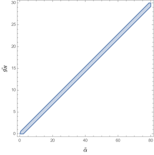
(a)

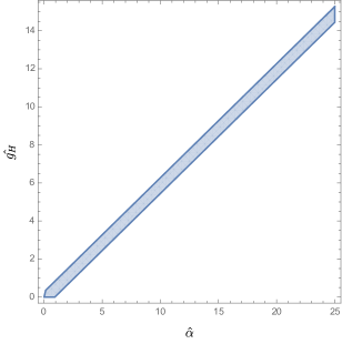
(b)

Figure 15: (a) The bounds on holographic QCD supported by the model in flat space Son:2003et (b) The bounds on holographic QCD from hard wall model in AdS Hirn:2005nr . All plots are still extending like a thin river.

It is important to note that the dictionary provides bounds uniformly scaled by $z_{\rm IR}$ or $R_{\rm AdS}$, both of which are the IR scales in QCD. From naive dimensional analysis, we expect them to be bounded by the bulk“string” scale $\Lambda$. This either means that this method yields bounds that are too weak, or that the IR RS branes disrupt the naive dimensional analysis. On the other hand, we found that even though we identify $R_{\rm AdS}$ with $z_{\rm IR}$, we can’t reproduce the flat-space scenario from the AdS one, which suggests a breakdown of the flat-space limit of causality bounds Caron-Huot:2021enk . It would be interesting to explore all these points in the future for a better understanding.

6 Summary

We reviewed the EFT bootstrap, especially for the positivity scenario. We demonstrated that the EFT bootstrap is essentially an infinite-dimensional SDP, where the optimization Lagrangian can be formulated. We built the dual problem of the EFT bootstrap using the crossing symmetric dispersive sum rules, which embrace the crossing symmetry without the IR danger, and thus it serves as a better version of the improved sum rules. For the primal problem of the EFT bootstrap, we adapted the S-matrix primal ansatz and optimized the target Wilson coefficients.

We then applied the EFT bootstrap program to large-$N$ $\chi$PT, which is a low-energy pion EFT from the chiral symmetry breaking of large-$N$ QCD. Due to the large-$N$ limit, the positivity EFT bootstrap is sufficiently strong to carve out the allowed EFT space. Our dual bounds match with earlier literature Albert:2022oes ; Fernandez:2022kzi , and we demonstrated that the primal bounds are also converging to the dual rigorous bounds. This is consistent with the strong duality of SDP. We then focused on some converged bounds and used the primal solutions to extract the physical spectrum and S-matrix that saturate those bounds. By doing this, we confirmed some of the analytic rule-in amplitudes studied in Albert:2022oes ; Fernandez:2022kzi . Interestingly, for the Skyrme bound, we also observed a mysterious heavy Regge trajectory, which seems to suggest meta-stable exotic states with heavy quarks. In addition, we showed that the Regge behaviour of the primal ansatz does not affect the bounds, if it stays below the assumed Regge boundedness. This is consistent with SDP, as the dual problem is only sensitive to the Regge boundedness rather than the explicit Regge behaviour. Eventually, we incorporated the upper bound of the unitarity, i.e., the linear unitarity EFT bootstrap to confirm that the large-$N$ limit is consistent.

In the end, we considered the holographic QCD models, which are EFTs of gauge fields in $5D$ and correspond to large-$N$ QCD in $4D$. Typically, we included the higher derivative terms in the bulk and showed that they give rise to the general chiral Lagrangian up to $\mathcal{O}(p^{4})$. We demonstrated that the Witten-Sakai-Sugimoto model with string corrections gives rise to a large-$N$ $\chi$PT within the allowed EFT region. Besides, for bottom-up models like the flat-space RS model and AdS hard-wall model, we translated the large-$N$ $\chi$PT to constrain the higher derivative couplings of ${\rm Tr}\,F^{3}$ and ${\rm Tr}\,F^{4}$ terms.

There are several aspects that deserve further investigations. From formal aspect, it would be interesting to build more precise relation between different methods for EFT and S-matrix bootstrap, include the SDP we reviewed, the moment problem Chiang:2021ziz ; Chiang:2022jep ; Chiang:2022ltp , geometric function Raman:2021pkf , iterative algorithm Tourkine:2023xtu ; Tourkine:2021fqh and machine learning approach Dersy:2023job . Focusing on the SDP perspective, typically, we state that the crossing symmetric sum rules are the more natural tools to understand the loop effects on the EFT bounds, since they are free of forward-limit issues. It is then interesting to make this statement concrete by using the crossing symmetric sum rules to study the scalar EFT, $\chi$PT and other EFTs, with one and even two loop effects, trying to make the results of Bellazzini:2021oaj ; Chala:2021wpj ; Li:2022aby sharp. For this exploration, it is also important to understand the primal-dual convergence when there are loops and the nonlinear unitarity is utilized. For example, we can apply the nonlinear unitarity bootstrap to real $\chi$PT like Guerrieri:2020bto ; He:2023lyy , and if the primal bounds and dual bounds converge, we can then probably extract the real QCD physics in the UV. Such analysis may also be extended to other important EFTs, like the standard model EFT Remmen:2019cyz ; Bi:2019phv ; Li:2022tcz ; Ghosh:2022qqq ; Chen:2023bhu , gravitational EFT Caron-Huot:2022ugt ; Caron-Huot:2022jli ; Noumi:2022wwf ; CarrilloGonzalez:2022fwg ; Chiang:2022jep ; deRham:2021bll , QCD string EFT EliasMiro:2019kyf , etc., helping us gain more information about their low-energy space as well as their possible UV completions.

Particularly for large-$N$ $\chi$PT, it remains puzzling to us that the Skyrme model is problematic above the kink, since the Skyrme model is a good phenomenological model for understanding many aspects of nuclear physics, e.g., Klebanov:1985qi ; Callan:1985hy . It would be interesting to understand, microscopically, how the Skyrme model goes wrong above the kink. A possible route is to study the pion-nuclei scattering, which can be described as pion fluctuations around the Skyrmion Saito:1985wd ; mattis1985baryon (which are solitons of the Skyrme model and serve as the baryon adkins1983static ; witten1979baryons ), and to detect if there are any causality violations like time advance Camanho:2014apa . Besides, it is also interesting to understand where our constraints on holographic QCD models come from in the bulk. The constraints may again arise from classical causality, and techniques from deRham:2021bll ; Chen:2021bvg ; CarrilloGonzalez:2022fwg ; CarrilloGonzalez:2023cbf ; Chen:2023rar would then be useful. This investigation may also be generalized to other RS scenarios, which provide the standard model EFTs.

Appendix A EFT bootstrap as SDP: more

In this appendix, we formulate the linear unitarity bootstrap and the nonlinear unitarity bootstrap as SDP.

A.1 Linear unitarity

For linear unitarity bootstrap, we write the Lagrangian as follows

$$\mathcal{L}_{g}=-\mathcal{F}\circ B(p^{2})-2(1-S+iT)\int_{M^{2}}^{\infty}\sum_{\rho}Y_{\rho}^{(2)}(s)\,,$$

$$\mathcal{F}\circ B(p^{2})=-g+\int_{M^{2}}^{\infty}ds\sum_{\rho}{\rm Im}\,a_{\rho}(s)\big{(}Y_{\rho}^{(1)}(s)-Y_{\rho}^{(2)}(s)\big{)}\,.$$ (125)

This SDP reads

• Primal

  $$\text{Minimize}\,\,g\,,\quad\text{Subject to}\,\,0\leq{\rm Im}\,a_{\rho}(s)\leq 2\,,S_{\rm free}=1\,.$$ (126)

• Dual

  $$\text{Maximize}\,\quad-2\int_{M^{2}}^{\infty}\sum_{\rho}Y_{\rho}^{(2)}(s)\,,\quad\text{Subject to}\,\,Y_{\rho}^{(i)}(s)\succeq 0\,.$$ (127)

A.2 Nonlinear unitarity

The nonlinear unitarity bootstrap is more subtle. From primal side, we have further requirement for real part of $a_{\rho}(s)$, however, such object does not appear in our dispersive sum rule. Nevertheless, one can shift the dispersion relation to finite $|s_{0}|>M$, we then have, for example for spin-$2$ sum rule

$$B_{2}(s_{0},p^{2})=\oint{\frac{ds}{4\pi i}}{\frac{2s+t}{(s_{0}-s)^{2}(s_{0}+s+t)^{2}}}=0\rightarrow$$

$$B_{2}(s_{0},p^{2})\Big{|}_{\text{low arc}}+{\frac{\mathcal{M}(s_{0},t)-\mathcal{M}(u_{0},t)+(2s_{0}+t)\partial_{s_{0}}\mathcal{M}(s_{0},t)}{2s_{0}+t}}+B_{2}(s_{0},p^{2})\Big{|}_{\rm high}=0\,.$$ (128)

We can then invert $\mathcal{M}(s_{0},t)$ to have $a_{\rho}(s)$, which is expressed in terms of complicated integral over low-energy contributions and UV part of the sum rules; schematically, we may have

$${\rm Re}\,a_{\rho}(s)\sim-i\,{\rm Im}\,a_{\rho}(s)+\int_{M^{2}}^{\infty}ds_{1}\int ds_{2}\mathcal{Y}_{\rho}(s_{1},s_{2}){\rm Im}\,a_{\rho}(s)+\text{low energy contribution}\,.$$ (129)

This type of relation can be used to build the functionals acting on ${\rm Re}\,a_{\rho}(s)$ by functionals acting on ${\rm Im}\,a_{\rho}(s)$ with double integrals. We then can write down the Lagrangian for nonlinear unitarity

$$\mathcal{L}_{g}=-\mathcal{F}\circ B(p^{2})-2(1-S+iT)\int_{M^{2}}^{\infty}\sum_{\rho}Y_{\rho}^{22}(s)-2\int_{M^{2}}^{\infty}ds\sum_{\rho}{\rm Re}\,a_{\rho}(s)Y_{\rho}^{12}(s)\,,$$

$$\mathcal{F}\circ B(p^{2})=-g+\int_{M^{2}}^{\infty}ds\sum_{\rho}{\rm Im}\,a_{\rho}(s)\big{(}Y_{\rho}^{11}(s)-Y_{\rho}^{22}(s)\big{)}\,.$$ (130)

In this Lagrangian, $Y^{11}$ and $Y^{22}$ can be constructed using the standard dispersive sum rules, while $Y_{\rho}^{12}(s)$ can only realized using intricate operations like (128) and (129) and contain double integral.

This SDP then reads

• Primal:

  $$\text{Minimize}\,\,g\,,\quad\text{Subject to}\,\,\mathcal{S}=\left(\begin{array}[]{cc}{\rm Im}\,a_{\rho}(s)&{\rm Re}\,a_{\rho}(s)\\ {\rm Re}\,a_{\rho}(s)&2-{\rm Im}\,a_{\rho}(s)\\ \end{array}\right)\succeq 0\,.$$ (133)

• Dual:

  Maximize $$-2\Big{(}\int_{M^{2}}^{\infty}\sum_{\rho}Y_{\rho}^{22}(s)+\int_{M^{2}}^{\infty}\sum_{\rho}{\rm Re}\,a_{\rho}(s)Y_{\rho}^{12}(s)\Big{)}\,,\quad\text{Subject to}$$

  $$Y=\left(\begin{array}[]{cc}Y_{\rho}^{11}(s)&Y_{\rho}^{12}(s)\\ Y_{\rho}^{12}(s)&Y_{\rho}^{22}(s)\\ \end{array}\right)\succeq 0\,.$$ (136)

Unfortunately, a more concrete dual example of this type of bootstrap is beyond the scope of this paper. We refer the readers to relevant discussions in Henriksson:2021ymi . It would be interesting to explicitly realize the dual algorithm we propose here and compare with other dual algorithm in the future Henriksson:2021ymi .

Appendix B Projectors of irreducible representation in SU$(N_{f})$

In this appendix, we record all the projectors of irreducible representation in SU$(N_{f})$ BandaGuzman:2020wrz that we used to organize the pion amplitudes.

$$P^{0}_{abcd}={\frac{1}{2N_{f}}}\delta_{ab}\delta_{cd}\,,\quad P^{{\rm adj}_{\rm A}}_{abcd}=-{\frac{1}{N_{f}}}f^{abe}f^{ecd}\,,\quad P^{{\rm adj}_{\rm S}}_{abcd}={\frac{N_{f}}{N_{f}^{2}-4}}d_{abe}d_{ecd}\,,$$

$$P^{\overline{a}s\oplus\overline{s}a}_{abcd}=-{\frac{1}{2}}\big{(}\delta_{ac}\delta_{bd}-\delta_{ad}\delta_{bd}\big{)}-{\frac{1}{N_{f}}}f_{abe}f_{ecd}\,,$$

$$P^{\overline{s}s}_{abcd}={\frac{N_{f}+2}{4N_{f}}}\big{(}\delta_{ac}\delta_{bd}+\delta_{ad}\delta_{bc}\big{)}-{\frac{N_{f}+2}{2N_{f}(N_{f}+1)}}\delta_{ab}\delta_{cd}-{\frac{N_{f}+4}{4(N_{f}+2)}}d_{abe}d_{ecd}+{\frac{1}{4}}\big{(}d_{abe}d_{ecd}+d_{cbe}d_{ead}\big{)}\,,$$

$$P^{\overline{a}a}_{abcd}={\frac{N_{f}-2}{4N_{f}}}\big{(}\delta_{ac}\delta_{bd}+\delta_{ad}\delta_{bc}\big{)}+{\frac{N_{f}-2}{2N_{f}(N_{f}-1)}}\delta_{ab}\delta_{cd}+{\frac{N_{f}-4}{4(N_{f}-2)}}d_{abe}d_{ecd}-{\frac{1}{4}}\big{(}d_{abe}d_{ecd}+d_{cbe}d_{ead}\big{)}\,.$$ (137)

Appendix C Fixing-parameter method

In this appendix, we explain the “fixing-parameter” method for nonlinearly bounding two Wilson coefficients, as a complementary of “angle-searching” method that was described in the main text.

The Lagrangian of “fixing-parameter method” is

$$\mathcal{L}=g_{1}+\lambda_{1}(g_{0}-1)+\lambda_{2}(g_{2}-g_{2}^{\ast})-\int_{M^{2}}^{\infty}ds\sum_{J}{\rm Im}\,a_{J}(s)Y_{J}(s)\,.$$ (138)

The interpretation is that we fix $g_{2}=g_{2}^{\ast}$ and bound $g_{1}$ in the unit of $g_{0}$. From dual method, this corresponds to having

$$\mathcal{F}\circ B(p^{2})\Big{|}_{\rm low}=-g_{1}-\lambda_{1}g_{0}-\lambda_{2}g_{2}\,,\quad{\rm maximize}\,\,\lambda_{1}+\lambda_{2}g_{2}^{\ast}\,,$$ (139)

which is precisely the fixing-parameter dual method used in Zhang:2021eeo . On the primal side, however, the implementation is a bit subtle. $g_{0}=1$ is the normalization condition in the primal algorithm, then how should we address $g_{2}=g_{2}^{\ast}$? Recall that any Wilson coefficients are linear combinations of the coefficients in primal ansatz that we aim to solve, this indicates that $g_{2}=g_{2}^{\ast}$ put more constraints on the primal ansatz. Effectively, the primal ansatz is then degenerate and the coefficients there are no longer all independent. The strategy is to make an matrix $R$ to reduce the anstaz to independent subspace so that

$$R\cdot g_{2}=g_{2}^{\ast}\,R\cdot g_{0}\,,$$ (140)

where we understand $g_{2}$ and $g_{0}$ as vectors spanned by the primal ansatz. Thus we can play with the effective Lagrangian

$$\mathcal{L}=R\cdot g_{1}+\lambda(R\cdot g_{0}-1)-\int_{M^{2}}^{\infty}ds\sum_{J}{\rm Im}\big{(}R\cdot a_{J}(s)\big{)}Y_{J}(s)\,.$$ (141)

References

- (1) H. Ooguri and C. Vafa, On the Geometry of the String Landscape and the Swampland, Nucl. Phys. B 766 (2007) 21–33, [hep-th/0605264].
- (2) T. D. Brennan, F. Carta and C. Vafa, The String Landscape, the Swampland, and the Missing Corner, PoS TASI2017 (2017) 015, [1711.00864].
- (3) E. Palti, The Swampland: Introduction and Review, Fortsch. Phys. 67 (2019) 1900037, [1903.06239].
- (4) M. van Beest, J. Calderón-Infante, D. Mirfendereski and I. Valenzuela, Lectures on the Swampland Program in String Compactifications, 2102.01111.
- (5) N. Arkani-Hamed, L. Motl, A. Nicolis and C. Vafa, The String landscape, black holes and gravity as the weakest force, JHEP 06 (2007) 060, [hep-th/0601001].
- (6) D. Harlow, B. Heidenreich, M. Reece and T. Rudelius, Weak gravity conjecture, Rev. Mod. Phys. 95 (2023) 035003, [2201.08380].
- (7) C. Cheung, J. Liu and G. N. Remmen, Proof of the Weak Gravity Conjecture from Black Hole Entropy, JHEP 10 (2018) 004, [1801.08546].
- (8) T. W. Grimm, E. Palti and I. Valenzuela, Infinite Distances in Field Space and Massless Towers of States, JHEP 08 (2018) 143, [1802.08264].
- (9) X. O. Camanho, J. D. Edelstein, J. Maldacena and A. Zhiboedov, Causality Constraints on Corrections to the Graviton Three-Point Coupling, JHEP 02 (2016) 020, [1407.5597].
- (10) A. Adams, N. Arkani-Hamed, S. Dubovsky, A. Nicolis and R. Rattazzi, Causality, analyticity and an IR obstruction to UV completion, JHEP 10 (2006) 014, [hep-th/0602178].
- (11) C. de Rham, S. Melville, A. J. Tolley and S.-Y. Zhou, Positivity bounds for scalar field theories, Phys. Rev. D 96 (2017) 081702, [1702.06134].
- (12) S. Caron-Huot and V. Van Duong, Extremal Effective Field Theories, JHEP 05 (2021) 280, [2011.02957].
- (13) A. J. Tolley, Z.-Y. Wang and S.-Y. Zhou, New positivity bounds from full crossing symmetry, 2011.02400.
- (14) N. Arkani-Hamed, T.-C. Huang and Y.-t. Huang, The EFT-Hedron, JHEP 05 (2021) 259, [2012.15849].
- (15) B. Bellazzini, J. Elias Miró, R. Rattazzi, M. Riembau and F. Riva, Positive moments for scattering amplitudes, Phys. Rev. D 104 (2021) 036006, [2011.00037].
- (16) L.-Y. Chiang, Y.-t. Huang, W. Li, L. Rodina and H.-C. Weng, Into the EFThedron and UV constraints from IR consistency, 2105.02862.
- (17) S. Caron-Huot, D. Mazac, L. Rastelli and D. Simmons-Duffin, Sharp Boundaries for the Swampland, JHEP 07 (2021) 110, [2102.08951].
- (18) S. Caron-Huot, D. Mazac, L. Rastelli and D. Simmons-Duffin, AdS bulk locality from sharp CFT bounds, JHEP 11 (2021) 164, [2106.10274].
- (19) S. Caron-Huot, Y.-Z. Li, J. Parra-Martinez and D. Simmons-Duffin, Causality constraints on corrections to Einstein gravity, JHEP 05 (2023) 122, [2201.06602].
- (20) S. Caron-Huot, Y.-Z. Li, J. Parra-Martinez and D. Simmons-Duffin, Graviton partial waves and causality in higher dimensions, Phys. Rev. D 108 (2023) 026007, [2205.01495].
- (21) J. Henriksson, B. McPeak, F. Russo and A. Vichi, Bounding violations of the weak gravity conjecture, JHEP 08 (2022) 184, [2203.08164].
- (22) D.-Y. Hong, Z.-H. Wang and S.-Y. Zhou, Causality bounds on scalar-tensor EFTs, 2304.01259.
- (23) A. Sinha and A. Zahed, Crossing Symmetric Dispersion Relations in QFTs, Phys. Rev. Lett. 126 (2021) 181601, [2012.04877].
- (24) L. Alberte, C. de Rham, S. Jaitly and A. J. Tolley, QED positivity bounds, 2012.05798.
- (25) X. Li, H. Xu, C. Yang, C. Zhang and S.-Y. Zhou, Positivity in Multifield Effective Field Theories, Phys. Rev. Lett. 127 (2021) 121601, [2101.01191].
- (26) Z. Bern, D. Kosmopoulos and A. Zhiboedov, Gravitational effective field theory islands, low-spin dominance, and the four-graviton amplitude, J. Phys. A 54 (2021) 344002, [2103.12728].
- (27) P. Haldar, A. Sinha and A. Zahed, Quantum field theory and the Bieberbach conjecture, SciPost Phys. 11 (2021) 002, [2103.12108].
- (28) P. Raman and A. Sinha, QFT, EFT and GFT, 2107.06559.
- (29) J. Henriksson, B. McPeak, F. Russo and A. Vichi, Rigorous Bounds on Light-by-Light Scattering, 2107.13009.
- (30) A. Zahed, Positivity and geometric function theory constraints on pion scattering, JHEP 12 (2021) 036, [2108.10355].
- (31) L. Alberte, C. de Rham, A. Momeni, J. Rumbutis and A. J. Tolley, Positivity Constraints on Interacting Spin-2 Fields, JHEP 03 (2020) 097, [1910.11799].
- (32) M. Accettulli Huber, A. Brandhuber, S. De Angelis and G. Travaglini, Eikonal phase matrix, deflection angle and time delay in effective field theories of gravity, Phys. Rev. D 102 (2020) 046014, [2006.02375].
- (33) L. Alberte, C. de Rham, S. Jaitly and A. J. Tolley, Reverse Bootstrapping: IR lessons for UV physics, 2111.09226.
- (34) S. D. Chowdhury, K. Ghosh, P. Haldar, P. Raman and A. Sinha, Crossing Symmetric Spinning S-matrix Bootstrap: EFT bounds, 2112.11755.
- (35) B. Bellazzini, M. Riembau and F. Riva, The IR-Side of Positivity Bounds, 2112.12561.
- (36) C. Zhang, SMEFTs living on the edge: determining the UV theories from positivity and extremality, 2112.11665.
- (37) Y.-J. Wang, F.-K. Guo, C. Zhang and S.-Y. Zhou, Generalized positivity bounds on chiral perturbation theory, JHEP 07 (2020) 214, [2004.03992].
- (38) T. Trott, Causality, Unitarity and Symmetry in Effective Field Theory, 2011.10058.
- (39) C. de Rham, S. Melville, A. J. Tolley and S.-Y. Zhou, UV complete me: Positivity Bounds for Particles with Spin, JHEP 03 (2018) 011, [1706.02712].
- (40) C. de Rham, S. Melville, A. J. Tolley and S.-Y. Zhou, Positivity Bounds for Massive Spin-1 and Spin-2 Fields, JHEP 03 (2019) 182, [1804.10624].
- (41) Z.-Y. Wang, C. Zhang and S.-Y. Zhou, Generalized elastic positivity bounds on interacting massive spin-2 theories, JHEP 04 (2021) 217, [2011.05190].
- (42) C. de Rham, S. Jaitly and A. J. Tolley, Constraints on Regge behavior from IR physics, Phys. Rev. D 108 (2023) 046011, [2212.04975].
- (43) T. Noumi and J. Tokuda, Finite energy sum rules for gravitational Regge amplitudes, JHEP 06 (2023) 032, [2212.08001].
- (44) J. Albert and L. Rastelli, Bootstrapping pions at large N, JHEP 08 (2022) 151, [2203.11950].
- (45) C. Fernandez, A. Pomarol, F. Riva and F. Sciotti, Cornering large-Nc QCD with positivity bounds, JHEP 06 (2023) 094, [2211.12488].
- (46) B. Bellazzini, G. Isabella, S. Ricossa and F. Riva, Massive Gravity is not Positive, 2304.02550.
- (47) J. Albert and L. Rastelli, Bootstrapping Pions at Large . Part II: Background Gauge Fields and the Chiral Anomaly, 2307.01246.
- (48) Q. Chen, K. Mimasu, T. A. Wu, G.-D. Zhang and S.-Y. Zhou, Capping the positivity cone: dimension-8 Higgs operators in the SMEFT, 2309.15922.
- (49) X. Li, Positivity bounds at one-loop level: the Higgs sector, JHEP 05 (2023) 230, [2212.12227].
- (50) G. Auberson and N. N. Khuri, Rigorous parametric dispersion representation with three-channel symmetry, Phys. Rev. D 6 (1972) 2953–2966.
- (51) G. Mahoux, S. M. Roy and G. Wanders, Physical pion pion partial-wave equations based on three channel crossing symmetry, Nucl. Phys. B 70 (1974) 297–316.
- (52) M. F. Paulos, J. Penedones, J. Toledo, B. C. van Rees and P. Vieira, The S-matrix bootstrap. Part III: higher dimensional amplitudes, JHEP 12 (2019) 040, [1708.06765].
- (53) L. Córdova and P. Vieira, Adding flavour to the S-matrix bootstrap, JHEP 12 (2018) 063, [1805.11143].
- (54) A. L. Guerrieri, J. Penedones and P. Vieira, Bootstrapping QCD Using Pion Scattering Amplitudes, Phys. Rev. Lett. 122 (2019) 241604, [1810.12849].
- (55) J. Elias Miró, A. L. Guerrieri, A. Hebbar, J. a. Penedones and P. Vieira, Flux Tube S-matrix Bootstrap, Phys. Rev. Lett. 123 (2019) 221602, [1906.08098].
- (56) L. Córdova, Y. He, M. Kruczenski and P. Vieira, The O(N) S-matrix Monolith, JHEP 04 (2020) 142, [1909.06495].
- (57) C. Bercini, M. Fabri, A. Homrich and P. Vieira, S-matrix bootstrap: Supersymmetry, , and symmetry, Phys. Rev. D 101 (2020) 045022, [1909.06453].
- (58) A. Guerrieri, J. Penedones and P. Vieira, Where Is String Theory in the Space of Scattering Amplitudes?, Phys. Rev. Lett. 127 (2021) 081601, [2102.02847].
- (59) A. Guerrieri, H. Murali, J. Penedones and P. Vieira, Where is M-theory in the space of scattering amplitudes?, JHEP 06 (2023) 064, [2212.00151].
- (60) D. Karateev, J. Marucha, J. a. Penedones and B. Sahoo, Bootstrapping the a-anomaly in 4d QFTs, JHEP 12 (2022) 136, [2204.01786].
- (61) J. K. Marucha, Bootstrapping the -anomaly in QFTs: Episode II, 2307.02305.
- (62) F. Acanfora, A. Guerrieri, K. Häring and D. Karateev, Bounds on scattering of neutral goldstones, 2023.
- (63) F. Acanfora, A. Guerrieri, K. Häring and D. Karateev, Bounds on scattering of neutral Goldstones, 2310.06027.
- (64) A. L. Guerrieri, J. Penedones and P. Vieira, S-matrix bootstrap for effective field theories: massless pions, JHEP 06 (2021) 088, [2011.02802].
- (65) H. Chen, A. L. Fitzpatrick and D. Karateev, Nonperturbative bounds on scattering of massive scalar particles in d 2, JHEP 12 (2022) 092, [2207.12448].
- (66) K. Häring, A. Hebbar, D. Karateev, M. Meineri and J. a. Penedones, Bounds on photon scattering, 2211.05795.
- (67) A. L. Guerrieri, A. Homrich and P. Vieira, Dual S-matrix bootstrap. Part I. 2D theory, JHEP 11 (2020) 084, [2008.02770].
- (68) A. Guerrieri and A. Sever, Rigorous Bounds on the Analytic S Matrix, Phys. Rev. Lett. 127 (2021) 251601, [2106.10257].
- (69) J. Elias Miro, A. Guerrieri and M. A. Gumus, Bridging positivity and S-matrix bootstrap bounds, JHEP 05 (2023) 001, [2210.01502].
- (70) H. Wolkowicz, R. Saigal and L. Vandenberghe, Handbook of semidefinite programming: theory, algorithms, and applications, vol. 27. Springer Science & Business Media, 2012.
- (71) S. R. Coleman and E. Witten, Chiral Symmetry Breakdown in Large N Chromodynamics, Phys. Rev. Lett. 45 (1980) 100.
- (72) G. ’t Hooft, A planar diagram theory for strong interactions, in The Large N Expansion In Quantum Field Theory And Statistical Physics: From Spin Systems to 2-Dimensional Gravity, pp. 80–92. World Scientific, 1993.
- (73) T. Ma, A. Pomarol and F. Sciotti, Bootstrapping the Chiral Anomaly at Large , 2307.04729.
- (74) Y. He and M. Kruczenski, Bootstrapping gauge theories, 2309.12402.
- (75) J. M. Maldacena, The Large N limit of superconformal field theories and supergravity, Adv. Theor. Math. Phys. 2 (1998) 231–252, [hep-th/9711200].
- (76) S. S. Gubser, I. R. Klebanov and A. M. Polyakov, Gauge theory correlators from noncritical string theory, Phys. Lett. B 428 (1998) 105–114, [hep-th/9802109].
- (77) E. Witten, Anti-de Sitter space and holography, Adv. Theor. Math. Phys. 2 (1998) 253–291, [hep-th/9802150].
- (78) E. Witten, Anti-de Sitter space, thermal phase transition, and confinement in gauge theories, Adv. Theor. Math. Phys. 2 (1998) 505–532, [hep-th/9803131].
- (79) T. Sakai and S. Sugimoto, Low energy hadron physics in holographic QCD, Prog. Theor. Phys. 113 (2005) 843–882, [hep-th/0412141].
- (80) T. Sakai and S. Sugimoto, More on a holographic dual of QCD, Prog. Theor. Phys. 114 (2005) 1083–1118, [hep-th/0507073].
- (81) M. Correia, A. Sever and A. Zhiboedov, An Analytical Toolkit for the S-matrix Bootstrap, 2006.08221.
- (82) S. Mizera, Physics of the Analytic S-Matrix, 2306.05395.
- (83) K. Häring and A. Zhiboedov, Gravitational Regge bounds, 2202.08280.
- (84) I. Buric, F. Russo and A. Vichi, Spinning Partial Waves for Scattering Amplitudes in Dimensions, 2305.18523.
- (85) Y. Hamada, R. Kuramochi, G. J. Loges and S. Nakajima, On (scalar QED) gravitational positivity bounds, JHEP 05 (2023) 076, [2301.01999].
- (86) L.-Y. Chiang, Y.-t. Huang, L. Rodina and H.-C. Weng, De-projecting the EFThedron, 2204.07140.
- (87) L.-Y. Chiang, Y.-t. Huang, W. Li, L. Rodina and H.-C. Weng, (Non)-projective bounds on gravitational EFT, 2201.07177.
- (88) D. Simmons-Duffin, A Semidefinite Program Solver for the Conformal Bootstrap, JHEP 06 (2015) 174, [1502.02033].
- (89) D. Poland and D. Simmons-Duffin, Bounds on 4D Conformal and Superconformal Field Theories, JHEP 05 (2011) 017, [1009.2087].
- (90) S. El-Showk and M. F. Paulos, Bootstrapping Conformal Field Theories with the Extremal Functional Method, Phys. Rev. Lett. 111 (2013) 241601, [1211.2810].
- (91) E. Witten, Current Algebra Theorems for the U(1) Goldstone Boson, Nucl. Phys. B 156 (1979) 269–283.
- (92) G. Veneziano, U(1) Without Instantons, Nucl. Phys. B 159 (1979) 213–224.
- (93) R. Kaiser and H. Leutwyler, Large N(c) in chiral perturbation theory, Eur. Phys. J. C 17 (2000) 623–649, [hep-ph/0007101].
- (94) J. Gasser and H. Leutwyler, Chiral Perturbation Theory to One Loop, Annals Phys. 158 (1984) 142.
- (95) J. Gasser and H. Leutwyler, Chiral perturbation theory: expansions in the mass of the strange quark, Nuclear Physics B 250 (1985) 465–516.
- (96) S. Peris and E. de Rafael, On the large-nc behaviour of the l7 coupling in pt, Physics Letters B 348 (1995) 539–542.
- (97) R. S. Chivukula, M. J. Dugan and M. Golden, Analyticity, crossing symmetry, and the limits of chiral perturbation theory, Physical Review D 47 (1993) 2930.
- (98) S. L. Adler, Consistency conditions on the strong interactions implied by a partially conserved axial-vector current, Physical Review 137 (1965) B1022.
- (99) V. M. Banda Guzmán, R. Flores-Mendieta, J. Hernández and F. d. J. Rosales-Aldape, Spin and flavor projection operators in the spin-flavor group, Phys. Rev. D 102 (2020) 036010, [2006.14169].
- (100) J. R. Pelaez and F. J. Yndurain, Regge analysis of pion pion (and pion kaon) scattering for energy s**1/2 1.4-GeV, Phys. Rev. D 69 (2004) 114001, [hep-ph/0312187].
- (101) J. R. Pelaez and F. J. Yndurain, The Pion-pion scattering amplitude, Phys. Rev. D 71 (2005) 074016, [hep-ph/0411334].
- (102) I. Low, R. Rattazzi and A. Vichi, Theoretical Constraints on the Higgs Effective Couplings, JHEP 04 (2010) 126, [0907.5413].
- (103) A. Falkowski, S. Rychkov and A. Urbano, What if the Higgs couplings to W and Z bosons are larger than in the Standard Model?, JHEP 04 (2012) 073, [1202.1532].
- (104) B. Bellazzini, L. Martucci and R. Torre, Symmetries, Sum Rules and Constraints on Effective Field Theories, JHEP 09 (2014) 100, [1405.2960].
- (105) W. Landry and D. Simmons-Duffin, Scaling the semidefinite program solver SDPB, 1909.09745.
- (106) V. G. Makhankov, Y. P. Rybakov and V. I. Sanyuk, The Skyrme Model: Fundamentals Methods Applications. Springer Science & Business Media, 2012.
- (107) F. Lenz, H. Griesshammer and D. Stoll, Lectures on QCD: Foundations. Springer, 1997.
- (108) J. J. Sakurai, Theory of strong interactions, Annals of Physics 11 (1960) 1–48.
- (109) B. McPeak, M. Venuti and A. Vichi, Adding subtractions: comparing the impact of different Regge behaviors, 2310.06888.
- (110) S. El-Showk, M. F. Paulos, D. Poland, S. Rychkov, D. Simmons-Duffin and A. Vichi, Solving the 3D Ising Model with the Conformal Bootstrap, Phys. Rev. D 86 (2012) 025022, [1203.6064].
- (111) D. T. Son and M. A. Stephanov, QCD and dimensional deconstruction, Phys. Rev. D 69 (2004) 065020, [hep-ph/0304182].
- (112) H.-C. Kim, Y. Kim and U. T. Yakhshiev, Hadrons from a hard wall AdS/QCD model, Chin. Phys. C 34 (2010) 1520–1522, [0912.1202].
- (113) J. Erlich, E. Katz, D. T. Son and M. A. Stephanov, QCD and a holographic model of hadrons, Phys. Rev. Lett. 95 (2005) 261602, [hep-ph/0501128].
- (114) L. Da Rold and A. Pomarol, Chiral symmetry breaking from five dimensional spaces, Nucl. Phys. B 721 (2005) 79–97, [hep-ph/0501218].
- (115) J. Hirn and V. Sanz, Interpolating between low and high energy QCD via a 5-D Yang-Mills model, JHEP 12 (2005) 030, [hep-ph/0507049].
- (116) G. Panico and A. Wulzer, Effective action and holography in 5D gauge theories, JHEP 05 (2007) 060, [hep-th/0703287].
- (117) P. Colangelo, J. J. Sanz-Cillero and F. Zuo, Holography, chiral Lagrangian and form factor relations, JHEP 11 (2012) 012, [1207.5744].
- (118) J. Erdmenger, N. Evans, I. Kirsch and E. Threlfall, Mesons in Gauge/Gravity Duals - A Review, Eur. Phys. J. A 35 (2008) 81–133, [0711.4467].
- (119) M. R. Pahlavani and R. Morad, Application of AdS/CFT in Nuclear Physics, Adv. High Energy Phys. 2014 (2014) 863268, [1403.2501].
- (120) M. Mia, K. Dasgupta, C. Gale and S. Jeon, Five Easy Pieces: The Dynamics of Quarks in Strongly Coupled Plasmas, Nucl. Phys. B 839 (2010) 187–293, [0902.1540].
- (121) V. Yadav, A. Misra and K. Sil, Delocalized SYZ Mirrors and Confronting Top-Down -Structure Holographic Meson Masses at Finite and with P(article) D(ata) G(roup) Values, Eur. Phys. J. C 77 (2017) 656, [1707.02818].
- (122) V. Yadav, G. Yadav and A. Misra, (Phenomenology/Lattice-Compatible) SU(3) MPT HD up to (p4) and the (R4)-Large-N Connection, JHEP 08 (2021) 151, [2011.04660].
- (123) L. Randall and R. Sundrum, A Large mass hierarchy from a small extra dimension, Phys. Rev. Lett. 83 (1999) 3370–3373, [hep-ph/9905221].
- (124) L. Randall and R. Sundrum, An Alternative to compactification, Phys. Rev. Lett. 83 (1999) 4690–4693, [hep-th/9906064].
- (125) A. Karch, E. Katz, D. T. Son and M. A. Stephanov, Linear confinement and AdS/QCD, Phys. Rev. D 74 (2006) 015005, [hep-ph/0602229].
- (126) T. Hagiwara, A NONABELIAN BORN-INFELD LAGRANGIAN, J. Phys. A 14 (1981) 3059.
- (127) A. Ballon-Bayona and L. A. H. Mamani, Nonlinear realization of chiral symmetry breaking in holographic soft wall models, Phys. Rev. D 102 (2020) 026013, [2002.00075].
- (128) A. Ballon-Bayona, L. A. H. Mamani and D. M. Rodrigues, Spontaneous chiral symmetry breaking in holographic soft wall models, Phys. Rev. D 104 (2021) 126029, [2107.10983].
- (129) S. Afonin and T. Solomko, Motivations for the Soft Wall holographic approach to strong interactions, 9, 2022. 2209.09042.
- (130) P. Tourkine and A. Zhiboedov, Scattering amplitudes from dispersive iterations of unitarity, 2303.08839.
- (131) P. Tourkine and A. Zhiboedov, Scattering from production in 2d, JHEP 07 (2021) 228, [2101.05211].
- (132) A. Dersy, M. D. Schwartz and A. Zhiboedov, Reconstructing -matrix Phases with Machine Learning, 2308.09451.
- (133) M. Chala and J. Santiago, Positivity bounds in the standard model effective field theory beyond tree level, Phys. Rev. D 105 (2022) L111901, [2110.01624].
- (134) G. N. Remmen and N. L. Rodd, Consistency of the Standard Model Effective Field Theory, JHEP 12 (2019) 032, [1908.09845].
- (135) Q. Bi, C. Zhang and S.-Y. Zhou, Positivity constraints on aQGC: carving out the physical parameter space, JHEP 06 (2019) 137, [1902.08977].
- (136) X. Li and S. Zhou, Origin of neutrino masses on the convex cone of positivity bounds, Phys. Rev. D 107 (2023) L031902, [2202.12907].
- (137) D. Ghosh, R. Sharma and F. Ullah, Amplitude’s positivity vs. subluminality: causality and unitarity constraints on dimension 6 & 8 gluonic operators in the SMEFT, JHEP 02 (2023) 199, [2211.01322].
- (138) M. Carrillo Gonzalez, C. de Rham, V. Pozsgay and A. J. Tolley, Causal effective field theories, Phys. Rev. D 106 (2022) 105018, [2207.03491].
- (139) C. de Rham, A. J. Tolley and J. Zhang, Causality Constraints on Gravitational Effective Field Theories, 2112.05054.
- (140) I. R. Klebanov, Nuclear Matter in the Skyrme Model, Nucl. Phys. B 262 (1985) 133–143.
- (141) C. G. Callan, Jr. and I. R. Klebanov, Bound State Approach to Strangeness in the Skyrme Model, Nucl. Phys. B 262 (1985) 365–382.
- (142) S. Saito, T. Otofuji and M. Yasuno, PION FLUCTUATIONS ABOUT THE SKYRMION, Prog. Theor. Phys. 75 (1986) 68–83.
- (143) M. P. Mattis and M. Karliner, Baryon spectrum of the skyrme model, Physical Review D 31 (1985) 2833.
- (144) G. S. Adkins, C. R. Nappi and E. Witten, Static properties of nucleons in the skyrme model, Nuclear Physics B 228 (1983) 552–566.
- (145) E. Witten, Baryons in the 1n expansion, Nuclear Physics B 160 (1979) 57–115.
- (146) C. Y. R. Chen, C. de Rham, A. Margalit and A. J. Tolley, A cautionary case of casual causality, 2112.05031.
- (147) M. Carrillo González, C. de Rham, S. Jaitly, V. Pozsgay and A. Tokareva, Positivity-causality competition: a road to ultimate EFT consistency constraints, 2307.04784.
- (148) C. Y. R. Chen, C. de Rham, A. Margalit and A. J. Tolley, Surfin’ pp-waves with Good Vibrations: Causality in the presence of stacked shockwaves, 2309.04534.