Classical shadow tomography with mutually unbiased bases

Abstract

Classical shadow tomography, harnessing randomized informationally complete (IC) measurements, provides an effective avenue for predicting many properties of unknown quantum states with sample-efficient precision. Projections onto $2^{n}+1$ mutually unbiased bases (MUBs) are widely recognized as minimal and optimal IC measurements for full-state tomography. We study how to use MUBs circuits as the ensemble in classical shadow tomography. For the general observables, the variance to predict their expectation value is shown to be exponential to the number of qubits $n$. However, for a special class termed as appropriate MUBs-average (AMA) observables, the variance decreases to $poly(n)$. Additionally, we find that through biased sampling of MUBs circuits, the variance for non-AMA observables can again be reduced to $poly(n)$ with the MUBs-sparse condition. The performance and complexity of using the MUBs and Clifford circuits as the ensemble in the classical shadow tomography are compared in the end.

I Introduction

In the realm of quantum information science, efficiently extracting information from unknown quantum states is pivotal. This is traditionally achieved through quantum state tomography [1, 2, 3], performing informationally complete (IC) measurements usually projected on $\{U_{j}|k\rangle,k=0,\cdots,d-1;j=1\cdots\}$, obtaining experimental data $\text{tr}(\rho U_{j}|k\rangle\langle k|U_{j}^{{\dagger}})$, then uniquely reconstructing density matrix $\rho$ with different methods. It allows for the prediction of various important functions $f(\rho)$, such as predicting the properties $\text{tr}(O\rho)$ under certain observable $O$, along with metrics like purity and entropy [4, 5, 6]. These predictions are central to many-body physics and quantum information theory [7, 8]. However, as quantum systems scale up, such as in the case of $n$-qubit quantum systems with dimension $d=2^{n}$, this method becomes impractical and even infeasible due to the enormous memory requirements.

Nevertheless, when computing specific functions $f(\rho)$, we can avoid the need to accurately calculate all elements of the density matrix with exponential measurements. While shadow tomography was initially proposed with polynomial sampling [9], it required exponential-depth quantum circuits applied to copies of all quantum states, presenting challenges for quantum hardware. Subsequently, Huang et al. introduced classical shadow tomography [10], enabling random measurements on individual quantum states and efficient prediction of various properties with a sampling complexity of  $\log(M)\|\cdot\|_{\text{norm}}^{2}$, where $M$ represents the number of observables, and $\|\cdot\|_{\text{norm}}^{2}$ denotes the norm of the corresponding observables. This norm is also influenced by the unitary ensemble $\{U_{j}\}$ we randomly choose.

The initial procedure applies random unitaries from a specific IC ensemble to the system and then performs computational projective measurements, which is equivalent to performing randomly $3^{n}$ Pauli measurements or all Clifford measurements. Pauli measurements are ideal for predicting localized target functions, while Clifford measurements excel in estimating functions with constant Hilbert-Schmidt norms, both offering valuable tools for various quantum tasks. Subsequently, various other ensembles have been explored, including fermionic Gaussian unitaries [11], chaotic Hamiltonian evolutions [12], locally scrambled unitary ensembles [13, 14, 15], and Pauli-invariant unitary ensembles [16]. The concept of randomly selecting multiple sets of projective measurements has been theoretically generalized to one POVM [17, 18]. Up to now, Classical shadow tomography has found applications in diverse fields, including energy estimation [19], entanglement detection [20, 21], and quantum chaos [22], quantum gate engineering cycle [23], and quantum error mitigation [24] to name a few.

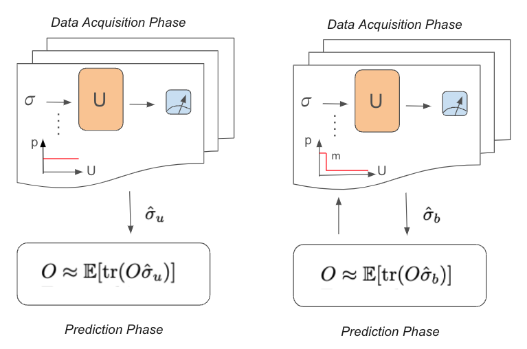
Figure 1: The procedure of the classical shadow tomography.

Without ancilla, the minimal number of IC ensemble contains $2^{n}+1$ unitary operations [25]. Projective measurements onto the set of $2^{n}+1$ mutually unbiased bases (MUBs) are recognized as the optimal approach for quantum tomography [25, 26, 27]. For a vector prepared within a specific MUB, a uniform distribution will be achieved when projecting it onto any other MUBs. These MUBs measurements are regarded as maximal incompatibility and complementarity [28], finding applications in various aspects of quantum information science, including quantum tomography [29, 30], uncertainty relations [31, 32, 33], quantum key distribution [34, 35], quantum error correction [36, 37, 38], as well as the identification of entanglement and other forms of quantum correlations [39, 40, 41, 42, 43, 44].

In this work, we use the MUBs as the unitary ensemble for classical shadow tomography. The reconstruction channel and the variance for MUBs are computed. We find that the variance for some bounded norm observables can be exponential with the number of qubits, but it can become polynomial when the observables (or state) are approximate MUBs-average (AMA). For observables that are not AMA but obey the MUBs-sparse condition, we show that by biased sampling, one can reduce the variance to polynomial order. The procedure of the classical shadow tomography based on MUBs circuits is summarized in Figure 1. In the end, we compare the algorithmic and circuit complexity of the MUBs and Clifford measurements.

II MUBs Classical shadow tomography

Let $A$ and $B$ be two Hermitian operators with normalized eigenstates $\{|a_{i}\rangle\}_{i=1}^{d}$ and $\{|b_{j}\rangle\}_{j=1}^{d}$. These two bases are called mutually unbiased if they satisfy the property

$$\lvert\langle a_{i}\lvert b_{j}\rangle\rvert^{2}=\frac{1}{d}$$ (1)

for all $i$ and $j$. For prime power $d$, there exist maximal ($d+1$) mutually unbiased bases (MUBs).

In $n$-qubit systems, the Hilbert space has a dimension of $d=2^{n}$. Denote the $2^{n}+1$ MUBs as $\{\mathcal{B}_{0},\cdots,\mathcal{B}_{2^{n}}\}$. Consider $\mathcal{B}_{0}$ as the canonical basis $\{|t\rangle\}_{t=0}^{2^{n}-1}$. Each additional basis is denoted as $\mathcal{B}_{j}=\{|e_{k}^{j}\rangle\}_{k=0}^{2^{n}-1}$. Utilizing the Galois-Fourier method, all basis states $|e_{k}^{j}\rangle$ are explicitly constructed [45]. Recently, each unitary operation $V_{j}=\sum_{k=0}^{2^{n}-1}|e_{k}^{j}\rangle\langle k|$ has been efficiently decomposed into $O(n^{2})$ elementary gates within $O(n^{3})$ time, structured as $-H-S-CZ-$ [46].

One of the nice properties of the MUBs is that the projective measurements onto them are informationally complete [27]. By utilizing these projections, we can construct $4^{n}$ orthogonal operations according to the Hilbert–Schmidt inner product, $\text{tr}(A^{{\dagger}}B)=(A,B)$. These operations can be constructed in the following manner:

• The initial $2^{n}$ operations stem from basis $\mathcal{B}_{0}$, represented as $\{|t\rangle\langle t|\}_{t=0}^{2^{n}-1}$.

• The remaining $4^{n}-2^{n}$ operations are generated from the bases $\{\mathcal{B}_{j}\}_{j=1}^{2^{n}}$. For each $j$, $2^{n}-1$ operations are constructed: $\{V_{j}|k\rangle\langle k|V_{j}^{{\dagger}}-I/2^{n}\}_{k=0}^{2^{n}-2}$.

II.1 Procedure

We can employ MUBs circuits as a unitary ensemble for conducting classical shadow tomography [10]. Consider $\sigma$ as the unknown quantum state and $O$ as the observable for prediction. The general procedure encompasses two primary steps.

The initial step involves generating classical shadows of state $\sigma$ utilizing MUBs measurements. We randomly select a $U_{j}$ from the $2^{n}+1$ MUBs circuits and rotate the unknown state, i.e., $\sigma\to U_{j}\sigma U_{j}^{{\dagger}}$. Here, $U_{j}=V_{j}^{{\dagger}}$. Subsequently, the qubits are measured on the computational basis. This measurement yields a 0/1 bit string of length $n$, denoted by $b_{0}\cdots b_{n-1}$. Let $k=b_{0}+2b_{1}+\cdots+b_{n-1}2^{n-1}$. We calculate the classical snapshot of $\sigma$, defined as

$$\hat{\sigma}=\mathcal{M}^{-1}(U_{j}^{{\dagger}}|k\rangle\langle k|U_{j})\;,$$ (2)

where $\mathcal{M}^{-1}$ represents the reconstruction channel depending on the chosen unitary ensemble. Interestingly, when uniformly sampling from MUBs circuits, the reconstruction channel mirrors that of Clifford circuits and can be expressed for any operator $X$ as

$$\mathcal{M}^{-1}_{\text{u}}(X)=(2^{n}+1)X-\text{tr}(X)I_{n}\;.$$ (3)

The specific calculations are detailed in Appendix A. Repeat this rotation-measurement process $N$ times. This yields a set of $N$ classical snapshots, termed a classical shadow of $\sigma$, which will be stored in the classical memory.

The second step involves using the obtained classical shadows to predict observables $\{O_{1},O_{2},\ldots,O_{M}\}$ of the unknown quantum state $\sigma$. Their expectation values are given by

$$o_{i}=\text{tr}(O_{i}\sigma),\quad 1\leq i\leq M\;,$$

which can be approximated by the median of means of the expectation values

$$\hat{o}_{i}(N,K)=\text{median}\{\hat{o}^{(1)}_{i}(L,1),\hat{o}^{(2)}_{i}(L,1),\ldots,\hat{o}^{(K)}_{i}(L,1)\}$$

where $L=\lfloor N/K\rfloor$ and

$$\hat{o}^{(k)}_{i}(L,1)=\frac{1}{L}\sum_{j=(k-1)L+1}^{kL}\text{tr}(O_{i}\hat{\sigma}_{j}),\quad 1\leq k\leq K\;.$$

This approximation depends on the choices of the parameters $L$ and $K$.

II.2 Performance

Suppose the unknown state is $\sigma$. To assess the performance of using MUBs-based classical shadow tomography to predict an observable $O$ under $\sigma$, one should examine the variance $\lVert O_{0}\rVert_{\sigma}^{2}$ in equation (4), where $O_{0}=O-\frac{\text{tr}(O)}{2^{n}}$ represents the traceless part of $O$. The sample complexity is linearly correlated with the variance.

$$\lVert O_{0}\rVert_{\sigma}^{2}=\mathbb{E}_{U\sim\mathcal{U}}\sum_{k=0}^{2^{n}-1}\langle k|U\mathcal{M}^{-1}(O_{0})U^{\dagger}|k\rangle^{2}\cdot\langle k|U\sigma U^{\dagger}|k\rangle$$ (4)

The variance for an arbitrary unknown state is defined by the shadow norm $\lVert O_{0}\rVert_{\text{shadow}}^{2}=\max_{\sigma:\text{state}}\lVert O_{0}\rVert_{\sigma}^{2}$. The variance of the shadow norm for Clifford and Pauli measurements has been studied in [10]. Now, we consider the shadow variance of the MUBs measurement. Using the result of the reconstruction channel in equation (3), it is straightforward to show that

$$\lVert O_{0}\rVert_{\sigma,\text{u}}^{2} =(2^{n}+1)\sum_{j=0}^{2^{n}}\sum_{k=0}^{2^{n}-1}\text{tr}^{2}(O_{0}P_{jk})\cdot\text{tr}(\sigma P_{jk})$$ (5)

where $P_{jk}=U_{j}^{{\dagger}}|k\rangle\langle k|U_{j}$. This variance depends exponentially on $n$ because the terms $\text{tr}(\sigma P_{jk})$ and $\text{tr}(O_{0}P_{jk})$ can take their maximal value $\sim O(1)$ at the same $j,k$. For example, when $O=|0\rangle\langle 0|$ and $\sigma=|0\rangle\langle 0|$, the variance is $\lVert O_{0}\rVert_{|0\rangle\langle 0|,\text{u}}^{2}\geq(2^{n}+1)(1-1/2^{n})^{2}$. Since each $0\leq\text{tr}(\sigma P_{jk})\leq 1$ for all $j,k$, we can derive that the variance $\max_{\sigma:\text{state}}\lVert O_{0}\rVert_{\sigma,\text{u}}^{2}\leq(2^{n}+1)\text{tr}(O_{0}^{2})$ for all $\sigma$ and $O$. Thus, when the unitary ensemble in the shadow tomography is MUBs circuits, to obtain an accurate enough prediction of $\langle O\rangle$, for the worst case, one needs to perform $\sim 2^{n}$ many samples.

A numerical experiment is performed. Consider the observable $O=|\text{GHZ}\rangle\langle\text{GHZ}|$ on the unknown state $|\text{GHZ}\rangle\langle\text{GHZ}|$. We predict the expectation value of $\langle O\rangle$, equivalently the fidelity between two GHZ states, for $n$ up to $8$ using shadows generated by $1000$ Pauli, Clifford, and MUBs measurements. The experiments are independently performed $10$ times. We plot the variance $\lVert O\rVert_{\sigma}$ in Figure 2, where the shaded area is the statistical variance between $10$ different random experiments. The results show that the variance of the prediction with shadows of Clifford measurements is independent of the number of qubits while for shadows obtained using Pauli and MUBs measurements, $\lVert O\rVert_{\sigma}$ scales exponential with $n$, which is consistent with the analysis made above.

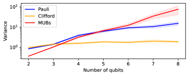
Figure 2: The variance of fidelity estimation between two GHZ states obtained from the shadows with different unitary ensembles. For each case, we randomly generate $10$ different shadows. The number of measurements in each shadow is $1000$. The shaded area is the statistical variance for $10$ independent experiments.

Although when the unitary ensemble is MUBs circuit, the variance $\lVert O_{0}\rVert_{\sigma,\text{u}}$ of the prediction $\langle O\rangle$ using classical shadow tomography depends exponentially with $n$, it can be shown that this variance can decrease to polynomial with $n$ when the interested observable $O$ or the unknown state $\sigma$ has the following property.

Definition 1 (Approximately MUBs-average).

A state $\sigma$ (or observable $O$) is called approximately MUBs-average (AMA) if it satisfies

$$|\text{tr}(\sigma P_{jk})-1/2^{n}|\leq\epsilon$$ (6)

for all $j,k$ and $\epsilon=O(poly(n))/2^{n}\ll 1$.

In other words, its probability distribution under each basis of MUBs is approximately uniform. Or if we express $\sigma$ with the $4^{n}$ orthogonal operations defined above, the matrix elements are all less than $\epsilon+1/2^{n}$. Here $\epsilon$ reflects the deviation from the MUBs-average state $I/2^{n}$ with $\epsilon=0$. $\lVert O_{0}\rVert_{I/d,\text{u}}^{2}=(1+1/2^{n})\text{tr}(O_{0}^{2})$. For $\epsilon=\frac{s}{2^{n}}\neq 0$, we can find many AMA states in the Hilbert space.

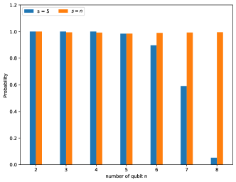
Figure 3: The percentage of AMA states with $\epsilon=s/2^{n}$ in $1000$ randomly chosen quantum states according to Haar measure in $n=2,3,\ldots,8$ qubit systems.

For example, we randomly generate $1000$ quantum states according to Haar measure in $n$-qubit system for $n=2,3,\ldots,8$. If we set $s=5$, we find that $89.7\%$ of these random states are AMA for $n=6$, $59\%$ for $n=7$, and $5.2\%$ for $n=8$. While for $n=2,3,4,5$, almost all these random states are AMA because $s=5$ is comparable with the $2^{n}$. However, if we increase it to $s=n$, almost all of these random states are AMA even for $n=8$. Thus, it seems that as long as we choose an approximate $s$ such that $\epsilon$ is large enough but still $\ll 2^{n}$, there are a large amount of AMA states in the Hilbert space.

Theorem 1.

If the observable $O$ is AMA, then for any unknown states $\sigma$, the upper bound of the variance is

$$\lVert O_{0}\rVert_{\sigma,\text{u}}^{2}\leq(1+\frac{1}{2^{n}})poly^{2}(n)\;.$$ (7)

On the other hand, if the unknown state $\sigma$ is AMA, then for any observable $O$ the variance is upper bounded by

$$\lVert O_{0}\rVert_{\sigma,\text{u}}^{2}\leq(1+\frac{1}{2^{n}})(1+poly(n))\text{tr}(O_{0}^{2})\;.$$ (8)

If $\text{tr}(O_{0}^{2})$ is constant bounded norm, then the variance is bounded by a polynomial function of $n$.

The proof of the theorem is left in Appendix B. Thus, if the observable is AMA or the unknown state happens to be AMA, the MUBs-based shadow tomography is an effective method to predict $\langle O\rangle$.

As an example, we study the expectation value $\langle O\rangle$ on the GHZ state for both AMA observable $O_{\text{AMA}}=|\phi\rangle\langle\phi|$ and non-AMA observable $O_{\text{GHZ}}=|\text{GHZ}\rangle\langle\text{GHZ}|$ for $n=2,3,\ldots,8$. Here, $|\phi\rangle$ are randomly chosen AMA states with $\epsilon=2/2^{n}$ for each $n$. By $1000$ MUBs measurements, we plot the variance of the prediction $\langle O\rangle$ in Figure 4. Compared with the $O_{\text{GHZ}}$ case, the variance of $O_{\text{AMA}}$ does not depends exponentially on $n$. Thus, it confirms our Theorem 1 and one can use the MUBs-based classical shadow tomography to predict the AMA observables.

Figure 4: The variance of fidelity estimation based on MUBs measurements. The unknown state is $|\text{GHZ}\rangle\langle\text{GHZ}|$. The observable is $O_{\text{GHZ}}=|\text{GHZ}\rangle\langle\text{GHZ}|$ (red) and $O_{\text{AMA}}=|\phi\rangle\langle\phi|$ (blue) where $|\phi\rangle$ are randomly chosen AMA states with $\epsilon=2/2^{n}$. The number of measurements in each shadow is $1000$. The shaded area is the statistical variance for $10$ independent experiments.

III Biased-MUBs classical shadow tomography

When both the unknown state $\sigma$ and observable $O$ are not AMA, the variance $\lVert O_{0}\rVert_{\sigma,\text{u}}^{2}$ could be exponential with $n$. To obtain an accurate prediction of $\langle O\rangle$, it requires $\sim 2^{n}$ MUBs measurements in classical shadow tomography. While, we find that if the observable $O=|\phi\rangle\langle\phi|$ or the unknown state $\sigma$ satisfies the MUBs-sparse condition, by the biased sampling, the variance can also be $poly(n)$.

Definition 2 (MUBs-sparse).

A state $|\phi\rangle$ is called MUBs-sparse if it has sparse expression under some basis $\mathcal{B}_{j}$. Precisely, $|\phi\rangle=\sum_{k=0}^{2^{n}-1}a_{k}U_{j}^{{\dagger}}|k\rangle$ for some $j$ and the nonzero elements in set $\{a_{k}:k=0,\cdots,2^{n}-1\}$ is $t=O(poly(n))$.

If a state is MUBs-sparse under basis $\mathcal{B}_{j}$, it is not AMA, as $\epsilon=O(1)$ under the measurement of $\mathcal{B}_{j}$. However, for the other $2^{n}$ bases, we can prove $\epsilon=t/2^{n}$ as follows.

Proposition 1.

Consider that $|\phi\rangle$ contains at most $t$ nonzero amplitudes under the expression of $\mathcal{B}_{j}$. For the other $2^{n}$ MUBs, we can prove $|\langle\phi|U_{j^{\prime}}|k\rangle|^{2}\leq t/2^{n}$, where $j^{\prime}\neq j$.

Proof.

We may as well express $|\phi\rangle=\sum_{k=1}^{t}a_{l_{k}}U_{j}^{{\dagger}}|l_{k}\rangle$. With the definition of MUBs, $|\langle k^{\prime}|U_{j^{\prime}}U_{j}^{{\dagger}}|l_{k}\rangle|=\frac{1}{\sqrt{2^{n}}}$ for $j\neq j^{\prime}$.

$$|\langle\phi|U_{j^{\prime}}|k\rangle|^{2} =\frac{1}{2^{n}}|\sum_{k=1}^{t}a_{l_{k}}e^{i\theta_{jk}}|^{2}$$

$$\leq\frac{1}{2^{n}}(\sum_{k=1}^{t}|a_{l_{k}}|^{2})(\sum_{k=1}^{t}|e^{i\theta_{jk}}|^{2})=\frac{t}{2^{n}}$$

∎

As we will see in the following, for MUBs-sparse observables, the variance of prediction can decrease significantly if one performs the MUBs measurements in a biased way. Our motivation to consider the biased sampling is from the observations in fidelity estimation between two GHZ states. In this case, both the unknown states and observable is not AMA but they are MUBs-sparse with $t=2$ under $\mathcal{B}_{0}$. If we sample the MUBs circuits $\{U_{i}\}_{i=0}^{d}$ uniformly in shadow tomography, the variance is exponential with $n$ from the Figure 2. In specific, $2000$ snapshots are enough to give $0.99$ fidelity for $n\leq 7$, but when $n\geq 8$, ensuring a fidelity of $0.95$ requires $10000$ samplings. Upon reviewing the numerical outcomes, we find that choosing more operation $U_{0}$ improves the estimated performance. Theoretically, $\text{tr}(O\mathcal{M}^{-1}(P_{0k}))=(2^{n}-1)/2$ when $U_{0}$ is chosen. If not, the expectation values could be $1/2^{n+1}-1/2$ or $1/2^{n}$. However, as $n$ exceeds 8, the likelihood of uniformly selecting $U_{0}$ drastically decreases. Appropriately increasing the number of samples of $U_{0}$ will result in a faster approximation of the exact expected value $1$.

Biased shadow tomography follows a similar process to the usual case, with the difference lying in the data acquisition phase—employing random MUBs measurements based on a biased distribution. For instance, if the observable $O=|\phi\rangle\langle\phi|$ is MUBs-sparse under $\mathcal{B}_{j}$, adjusting probabilities can prioritize sampling from $U_{j}$ while reducing others’ likelihood, as outlined below.

$$p_{U_{j}}=\frac{1}{2^{n}+1}\to\frac{1+m}{2^{n}+1+m},\qquad U_{j}$$

$$p_{U_{k}}=\frac{1}{2^{n}+1}\to\frac{1}{2^{n}+1+m},\qquad$$ otherwise (9)

where $m$ is a real number. Note that when we use the biased shadow to predict $\langle O\rangle$, the variance for uniform sampling in equation (5) does not apply anymore. In fact, the correct variance depends on the parameter $m$. As we will see later, $m$ is not a free parameter in our scheme but will be fixed to be the one that minimizes this variance.

When we randomly sample the MUBs circuits according to equation (III), for any operator $X$, the reconstruction channel becomes

$$\mathcal{M}_{b}^{-1}(X)=(2^{n}+1+m)[X-\frac{m}{1+m}\text{tr}(XP_{jk})P_{jk}]-\frac{\text{tr}(X)I}{1+m}.$$ (10)

When $m=0$, it becomes the reconstruction channel for the uniform sampling case in equation (3) and $\mathcal{M}_{b}^{-1}(X)=\mathcal{M}_{u}^{-1}(X)$. The details of this derivation can be found in Appendix A.

Theorem 2.

Given an observable $O=|\phi\rangle\langle\phi|$ and unknown quantum state $\sigma$, if $|\phi\rangle$ is MUBs-sparse, one can efficiently predict $\langle O\rangle$ using biased MUBs sampling. The upper bound of variance is given by

$$\lVert O_{0}\rVert_{\sigma,b}^{2}\leq t^{2},\;\text{~{}when~{}}\;m=\frac{2^{n}}{t-1}-1.$$ (11)

and the optimal probabilities to choose $U_{j}$ and the other unitary circuits in the MUBs-set are

$$p_{U_{j}}=\frac{1}{t};\qquad p_{U_{k}}=\frac{1}{2^{n}}\left(1-\frac{1}{t}\right),\quad k\neq j$$ (12)

On the other hand, given an observable $O$ and unknown quantum state $\sigma=|\phi\rangle\langle\phi|$, if $|\phi\rangle$ is MUBs-sparse, one can predict $\langle O\rangle$ using biased MUBs sampling. The upper bound of variance is given by

$$\lVert O_{0}\rVert_{\sigma,b}^{2}\leq(\sqrt{t}+1)^{2}\text{tr}(O_{0}^{2}),\;\text{when }\;m=\frac{2^{n}}{\sqrt{t}}-1.$$ (13)

and the optimal probabilities to choose $U_{j}$ and the other unitary circuits in the MUBs-set are

$$p_{U_{j}}=\frac{1}{1+\sqrt{t}};\qquad p_{U_{k}}=\frac{1}{2^{n}}\left(\frac{1}{1+\sqrt{t}}\right),\quad k\neq j$$ (14)

The proof is left in the Appendix B. For both cases, the variance for predicting the MUBs-sparse observable is upper bounded by a function independent of $n$. Thus, classical shadow tomography based on the MUBs circuits works not only for AMA observables but also for observables that are MUBs-sparse by biased sampling.

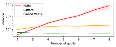
Figure 5: The variance of fidelity estimation between two GHZ states using MUBs shadows (red), Clifford shadows (orange), and Biased MUBs shadows (green). The shaded region is the statistical variance among $10$ randomly generated shadows. The number of measurements in each shadow is $1000$.

Let’s consider the fidelity estimation between two GHZ states again. In Figure 5, we compare the variance of the predictions of $O_{\text{GHZ}}$ using the shadows obtained by Clifford, MUBs and biased MUBs measurements. As discussed before, the observable is not AMA. Uniform sampling in the shadow tomography leads to the exponential dependence of $n$ in the variance. While since $O_{\text{GHZ}}$ is MUBs-sparse with $t=2$ under $U_{0}=I$, according to Theorem 2, we perform the MUBs measurements in a biased ways with the probability $0.5$ on $U_{0}$ and $1/2^{n+1}$ on the others. By doing so, the variance decreases significantly that is even lower than the Clifford case. In this simple example, we have shown that by biased sampling, the classical shadow tomography based on MUBs circuits works for the MUBs-sparse observables.

Remark.

Note that for observables that can be treated as the density matrix of mixed states i.e. $O=\sum_{k=1}^{s}p_{k}|\phi_{k}\rangle\langle\phi_{k}|$ with $p_{k}\geq 0$ and $\sum_{k=1}^{s}p_{k}=1$, if all $\{|\phi_{k}\rangle\}$ are MUBs-sparse under the same basis $\mathcal{B}_{j}$, then the theorem 2 still holds.

It is easy to check that $\text{tr}(OP_{j^{\prime}k})\leq\frac{t}{2^{n}}$ for each $k$ when $j^{\prime}\neq j$.

IV Comparison with random Clifford measurements

Based on the performance of the classical shadow tomography with MUBs ensemble, we classify the quantum states (observables) into three classes as depicted in Figure (6). With uniform MUBs circuit sampling, we observe that the worst-case variance is bounded by $(2^{n}+1)\text{tr}(O_{0})^{2}$, while the average variance is $(1+1/2^{n})\text{tr}(O_{0})^{2}$. Notably, for AMA states (observables), the variance remains polynomial. Additionally, with biased MUBs circuit sampling, the variance for sparse states (observables) also stays polynomial. By contrast, when employing uniform sampling of Clifford circuits, the variance for all states (observables) is limited to $3\text{tr}(O_{0}^{2})$.

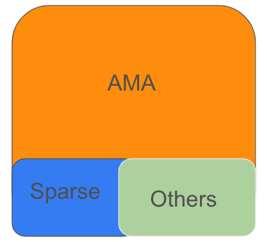
Figure 6: States classification. We divide all $n$-qubit states into three parts, AMA states (observables), states (observables) with a ‘sparse’ representation under some basis $\mathcal{B}_{j}$, and others. It’s intriguing to explore if other states share similar properties with the sparse states and to assess the percentage of these failed states within the complete set.

In addition to the performance, experiment implementation and post-processing are two main procedures in classical shadow tomography. We compare them for Clifford ensembles and MUBs ensembles.

Experiment implementation

In the data acquisition phase, one needs to randomly sample the unitary operations in the ensemble many times. The MUBs ensemble has much fewer elements compared with the Clifford one, thus making the sampling process more direct. Also, the random MUBs circuit structure is simpler to implement in the experiments than the random Clifford circuit. Surprisingly, we only need to consider $n$ special MUBs circuit to implement all.

• Sampling process

  As for the $n$-qubit Clifford ensemble, the number of elements is $2^{n^{2}+2n}\prod_{j=1}^{n}(4^{j}-1)$. The quantity is too large to sample directly from the first to the last. Nevertheless, each Clifford circuit $U$ is fully characterized by its action on $2^{n}$ Pauli operators [47]: $UX_{j}U^{\dagger}=(-1)^{r_{j}}\prod_{i=1}^{n}X_{i}^{\alpha_{ji}}Z_{i}^{\beta_{ji}}$, and $UZ_{j}U^{\dagger}=(-1)^{s_{j}}\prod_{i=1}^{n}X_{i}^{\gamma_{ji}}Z_{i}^{\delta_{ji}}$. The parameters that define $U$ are $(\alpha,\beta,\gamma,\delta,r,s)$, where $\alpha,\beta,\gamma,\delta$ are $n\times n$ matrices of bits, and $r,s$ are $n$-bit vectors. Given these parameters, different methods can decompose $U$ into elementary circuits [47, 48, 49, 50, 51, 52]. The time complexity is $O(n^{3})$ or $O(n^{2})$, while the number of elementary gates is $O(n^{2}/\log n)$ or $O(n^{2})$.

  As for the $n$-qubit MUBs ensemble, there are $2^{n}+1$ circuits. This allows for a direct uniform (biased) sampling due to their significantly lower count compared to Clifford circuits. In paper [46], $2^{n}+1$ circuits $\{I,U(0),U(1),\cdots,U(2^{n}-1)\}$ produce $2^{n}+1$ MUBs by acting on computational basis. The sampled MUBs circuits are $\{I,U^{{\dagger}}(0),\cdots,U^{{\dagger}}(2^{n}-1)\}$. Each nontrivial circuit $U(j)$ is obtained within $O(n^{3})$ time. Notably, every circuit comprises at most $(n^{2}+7n)/2$ elementary gates. On average, the counts of gates includes $3n/2$ $S$ gates, $(n^{2}-n)/4$ $CZ$ gates, and $(n-u)/2$ $CZ$ gates with a distance $u$.

• Circuits structure

  For the Clifford ensemble, the circuit is structured with 11-stage decomposition: $-H-CX-S-CX-S-CX-H-S-CX-S-CX-$ [48], or 7-stage decomposition: $-CX-CZ-S-H-S-CZ-CX-$ [50, 52].

  For the MUBs ensemble, the circuit is structured by $-H-S-CZ-$. The entanglement $CZ$ component consists of $2n-3$ fixed modules. Furthermore, the structures among different MUBs circuits exhibit a strong correlation. Linear relations exist in these $2^{n}+1$ MUBs circuits. Each $U(j)$ can be derived from the following $n$ circuits: $\{U(2^{0}),U(2^{1}),\cdots,U(2^{n-1})\}$.

Post-processing

In the prediction phase, we require two sets of data: the unitary operations used in the rotation, $U_{j}$, and the measurement outcomes, $|k\rangle$. With them, one can estimate the expected value of observable $O$ by

$$o\approx\text{tr}[\mathcal{M}^{-1}(U_{j}^{{\dagger}}|k\rangle\langle k|U_{j})O]\;.$$ (15)

However, as $n$ grows, the evaluation of the above expression becomes exponentially slow. This challenge is evident for Clifford circuits when the observable $O$ lacks efficient representations, such as an efficient stabilizer decomposition. For MUBs circuits, a similar issue may arise when $O$ lacks a sparse representation under some basis $\mathcal{B}_{j}$.

In the case of Clifford ensembles, the number of all stabilizer states ${U_{j}^{{\dagger}}|k\rangle}$ is $O(2^{n^{2}/2})$, while the number of MUBs states is $2^{n}(2^{n}+1)$. Consequently, the number of possible classical snapshots in equation (2) decreases for MUBs ensembles. Although the set of all MUBs states is a subset of all stabilizer states, the Clifford ensembles prove effective for a broader range of observables, considering the computational complexity involved in obtaining the estimation $o$.

The circuit decomposition can be realized in all physical platforms. In a quantum optical experiment, one could perform the random Clifford measurements by uniformly projecting a stabilizer state $U^{{\dagger}}_{j}|k\rangle$. To compute all these $2^{n}$ coefficients, the time complexity is $O(n\cdot 2^{3n})$ when we use the exression of stabilizers generators $\{g_{i}\}_{i=1}^{n}$, where $U^{{\dagger}}_{j}|k\rangle\langle k|U^{{\dagger}}_{j}=\frac{1}{2^{n}}\prod_{i=1}^{n}(I+g_{i})$. A new approach reduces the complexity to $O(2^{n}n^{3})$ [53]. If we randomly project a MUBs state $U(j)|k\rangle$, the time complexity is also $O(2^{n}n^{3})$ and one can directly calculate the coefficients [45, 46].

$$U(j)|k\rangle=|f_{k}^{j}\rangle=\frac{1}{\sqrt{2^{n}}}\sum_{l=0}^{2^{n}-1}|l\rangle(-1)^{k\cdot l^{T}}\cdot\alpha_{l}^{j}$$

where $\alpha_{l}^{j}=\prod_{s,t=0}^{n-1}\overline{(\sqrt{-1})^{j\odot(l_{s}\cdot 2^{s})\odot(l_{t}\cdot 2^{t})}}$ and $k$ ranges from $0$ to $2^{n}-1$.

V Conclusion

In this paper, we explore classical shadow tomography by uniform and biased sampling MUBs circuits. The $2^{n}+1$ MUBs is the minimal and optimal set for full $n$-qubit state tomography, which also constitutes a subset of all Clifford circuits. MUBs circuit is structured with 3-stage decomposition $-H-S-CZ-$ [46], a part of Clifford circuit [52]. There are ‘linear’ relations between these MUBs circuits and the average number of different gates can be counted.

The reconstruction channel and variance are calculated for random uniform and biased sampling of MUBs circuits. For the most general observable, the variance is bounded by $O(2^{n})$, but if one considers a special subset defined as AMA observables, we show that the upper bound of the variance becomes $poly(n)$ which is comparable with the Clifford case. Furthermore, we find that by biased sampling of MUBs circuits, we can effectively decrease the variance to $poly(n)$ when the observable (or the unknown state) is MUBs-sparse. All these results are demonstrated by the numerical experiments.

There are many future directions that one can pursue with the classical shadow tomography with MUBs circuits. First, we would like to find an efficient scheme to predict the general observables that are not AMA and MUBs-spares. Second, it’s interesting to consider more types of observables like two-point correlation functions and OTOCs. Third, one can also study how to use the MUBs circuits to predict nonlinear or polynomial observables such as entanglement entropy.

Acknowledgements— The work of Yu Wang received support from the National Natural Science Foundation of China through Grants No. 62001260 and No. 42330707, as well as from the Beijing Natural Science Foundation under Grant No. Z220002. The work of Wei Cui is supported by the fellowship of China Postdoctoral Science Foundation NO.2022M720507 and in part by the Beijing Postdoctoral Research Foundation.

Appendix A Computation details of the reconstruction channel

In the classical shadow tomography, after a MUBs measurements $\{U_{j}^{{\dagger}}|k\rangle\langle k|U_{j}\}_{k=0}^{2^{n}-1}$, the unknown density matrix $\rho$ can be viewed as collapsing to $P_{jk}=U_{j}^{{\dagger}}|k\rangle\langle k|U_{j}$ with $|k\rangle$ a state in the computational basis. To obtain the classical shadows $\hat{\rho}$, one needs to know the reconstruction channel $\mathcal{M}^{-1}$. We calculate the reconstruction channels of the MUBs measurements for both uniform and biased samplings. The computation details are given below.

Uniform sampling

The channel of the MUBs measurements is defined in the following way.

$$\mathcal{M}_{\text{u}}(\rho)=\frac{1}{{2^{n}+1}}\sum_{j=0}^{2^{n}}\sum_{k=0}^{2^{n}-1}\mbox{tr}(\rho P_{jk})\cdot P_{jk}$$ (16)

As the MUBs circuits are informationally complete, each $\rho$ can be expressed with the form of

$$\rho=\sum_{j=0}^{2^{n}}\sum_{k=0}^{2^{n}-1}x_{jk}P_{jk}.$$

Note here the coefficients $\{x_{jk}\}$ may not be unique. It is straightforward to show that

$$\mbox{tr}(\rho P_{jk}) =\mbox{tr}[(\sum_{a=0}^{2^{n}}\sum_{b=0}^{2^{n}-1}x_{ab}P_{ab})\cdot P_{jk}]$$ (17)

$$=(\sum_{a=j,b=k}+\sum_{a=j,b\neq k}+\sum_{a\neq j})\mbox{tr}[(x_{ab}P_{ab}\cdot P_{jk}]$$ (18)

$$=x_{jk}+\underbrace{0+\ldots+0}_{2^{n}-1}+\frac{1}{2^{n}}\sum_{a\neq j}\sum_{b=0}^{2^{n}-1}x_{ab}$$ (19)

$$=x_{jk}+\frac{1}{2^{n}}\sum_{a=0}^{2^{n}}\sum_{b=0}^{2^{n}-1}x_{ab}-\frac{1}{2^{n}}\sum_{b=0}^{2^{n}-1}x_{jb}$$ (20)

$$=x_{jk}+\frac{1}{2^{n}}\mbox{tr}(\rho)-\frac{1}{2^{n}}\sum_{b=0}^{2^{n}-1}x_{jb}$$ (21)

Here in equation (19) we use the property in equation (1), i.e. the square of the inner product of each two eigenstates in different MUBs is $1/2^{n}$.

$$\mathcal{M}_{\text{u}}(\rho) =\frac{1}{{2^{n}+1}}\sum_{j=0}^{2^{n}}\sum_{k=0}^{2^{n}-1}(x_{jk}+\frac{\text{tr}(\rho)}{2^{n}}-\frac{1}{2^{n}}\sum_{b=0}^{2^{n}-1}x_{jb})\cdot P_{jk}$$ (22)

$$=\frac{1}{{2^{n}+1}}(\rho+\frac{\text{tr}(\rho)(2^{n}+1)I}{2^{n}}-\sum_{j=0}^{2^{n}}\sum_{b=0}^{2^{n}-1}\frac{x_{jb}}{2^{n}}I)$$ (23)

$$=\frac{1}{{2^{n}+1}}(\rho+\frac{\text{tr}(\rho)(2^{n}+1)I}{2^{n}}-\frac{\mbox{tr}(\rho)}{2^{n}}I)$$ (24)

$$=\frac{1}{{2^{n}+1}}(\rho+\text{tr}(\rho)I)$$ (25)

Then the inverse channel is given by

$$\mathcal{M}_{\text{u}}^{-1}(\rho)=(2^{n}+1)\rho-\text{tr}(\rho)I.$$ (26)

It is the same as the reconstruction channel for the Clifford measurements [10].

Biased sampling

Without loss of generality, we may as well let the biased sampling basis be $\mathcal{B}_{0}$. The sampling probability is $\frac{1+m}{2^{n}+1+m}$ for $U_{0}=I$, and the sampling probability for other $U_{j}$ is $\frac{1}{2^{n}+1+m}$ where $j\neq 0$. The resulting reconstruction channel for this adjusted sampling process will be

$$\mathcal{M}_{\text{b}}(\rho) =\frac{1}{{2^{n}+1+m}}[\sum_{j=0}^{2^{n}}\sum_{k=0}^{2^{n}-1}\mbox{tr}(\rho P_{jk})\cdot P_{jk}+m\sum_{k=0}^{2^{n}-1}\mbox{tr}(\rho P_{0k})\cdot P_{0k}]$$ (27)

$$=\frac{1}{{2^{n}+1+m}}[\rho+\text{tr}(\rho)I+m\sum_{k=0}^{2^{n}-1}\mbox{tr}(\rho P_{0k})\cdot P_{0k}]$$ (28)

Then the updated inverse channel will be

$$\mathcal{M}_{\text{b}}^{-1}(\rho)=(2^{n}+1+m)[\rho-\frac{m}{1+m}\sum_{k}\text{tr}(\rho P_{0k})P_{0k}]-\frac{\text{tr}(\rho)I}{1+m}.$$ (29)

Appendix B Computational details on the variance

The performance of the classical shadow tomography is linear dependent with the variance defined below

$$\lVert O-\frac{\text{tr}(O)}{2^{n}}\rVert_{\text{ shadow}} =\max_{\sigma:\text{ state }}\left(\mathbb{E}_{U\sim\mathcal{U}}\sum_{b\in\{0,1\}^{n}}\langle b|U\sigma U^{\dagger}|b\rangle\cdot\langle b|U\mathcal{M}^{-1}(O-\frac{\text{tr}(O)}{2^{n}})U^{\dagger}|b\rangle^{2}\right)^{1/2}$$ (30)

where $U$ is a randomly chosen circuit in the unitary ensemble $\mathcal{U}$. From the definition, the variance depends on the observable $O$ and choice of the $\mathcal{U}$, but it also depends implicitly on how one samples the circuits. In this section, we calculate this variance when $\mathcal{U}$ is MUBs circuits for both uniform and biased sampling.

Uniform sampling

For the traceless part $O_{0}=O-\frac{\text{tr}(O)}{2^{n}}$, we know $\text{tr}(O_{0})=0$. The reconstruction channel is

$$\mathcal{M}_{\text{u}}^{-1}(O_{0})=(2^{n}+1)O_{0}-\text{tr}(O_{0})I=(2^{n}+1)O_{0}$$

One obtains that

$$\lVert O_{0}\rVert_{\text{ shadow}}^{2} =\max_{\sigma:\text{ state }}\lVert O_{0}\rVert_{\sigma,\text{u}}^{2}$$ (31)

$$=\max_{\sigma:\text{ state }}\frac{1}{2^{n}+1}\sum_{j=0}^{2^{n}}\sum_{k=0}^{2^{n}-1}\text{tr}(\sigma P_{jk})\cdot\text{tr}^{2}((2^{n}+1)O_{0}P_{jk})$$ (32)

$$=\max_{\sigma:\text{ state }}(2^{n}+1)\sum_{j=0}^{2^{n}}\sum_{k=0}^{2^{n}-1}\text{tr}^{2}(O_{0}P_{jk})\cdot\text{tr}(\sigma P_{jk})$$ (33)

Proposition 2.

$\sum_{j,k}\text{tr}^{2}(O_{0}P_{jk})=\text{tr}(O_{0}^{2})$.

Proof.

By equation (16), we have

$$\sum_{j=0}^{2^{n}}\sum_{k=0}^{2^{n}-1}\text{tr}(O_{0}P_{jk})\cdot P_{jk}=(2^{n}+1)\mathcal{M}({O_{0}})=O_{0}-\text{tr}(O_{0})I=O_{0}$$ (34)

Thus $\sum_{j,k}\text{tr}(O_{0}P_{jk})=\text{tr}(O_{0})=0$.

Define $O_{0,j}=\sum_{k=0}^{2^{n}-1}\text{tr}(O_{0}P_{jk})P_{jk}$, thus $O_{0}=\sum_{j}O_{0,j}$. It is easy to prove $\text{tr}(O^{2}_{0,j})=\sum_{k=0}^{2^{n}-1}\text{tr}^{2}(O_{0}P_{jk})$. If $j\neq j^{\prime}$, we have

$$\text{tr}(O_{0,j}O_{0,j^{\prime}}) =\frac{1}{2^{n}}\sum_{k,k^{\prime}}\text{tr}(O_{0}P_{jk})\text{tr}(O_{0}P_{j^{\prime}k^{\prime}})$$ (35)

$$=\frac{1}{2^{n}}\text{tr}(O_{0}\sum_{k}P_{jk})\text{tr}(O_{0}\sum_{k^{\prime}}P_{j^{\prime}k^{\prime}})$$ (36)

$$=0$$ (37)

Here we use $\text{tr}(O_{0}I)=0$. Thus $\text{tr}(O_{0}^{2})=\sum_{j}\text{tr}(O^{2}_{0,j})=\sum_{j}\sum_{k}\text{tr}^{2}(O_{0}P_{jk})$. ∎

Now, we give the proof of equation (7).

Proof.

As $\text{tr}(\sigma P_{jk})\leq\epsilon+\frac{1}{2^{n}}$ for all $j,k$, we have $\lVert O_{0}\rVert_{\sigma,\text{u}}^{2}\leq(2^{n}+1)(\epsilon+\frac{1}{2^{n}})\sum_{j,k}\text{tr}^{2}(O_{0}P_{jk})=(2^{n}+1)(\epsilon+\frac{1}{2^{n}})\text{tr}(O_{0}^{2})$. Thus $\lVert O_{0}\rVert_{\sigma,\text{u}}^{2}\leq(1+\frac{1}{2^{n}})(1+poly(n))\text{tr}^{2}(O_{0})$.

When $\epsilon=O(1/2^{n})$ and $\text{tr}(O_{0}^{2})$ is bounded, the variance for these states $\sigma$ is at a constant level. When $\sigma=I/2^{n}$ we have $\epsilon=0$ and $\lVert O_{0}\rVert_{\sigma}^{2}\leq\frac{2^{n}+1}{2^{n}}\text{tr}(O_{0}^{2})$. ∎

Here, we give the proof of equation (8).

Proof.

As $\text{tr}(O_{0}P_{jk})=\text{tr}(OP_{jk})-1/2^{n}$, we have $\text{tr}^{2}(O_{0}P_{jk})\leq\epsilon^{2}$. Then $\lVert O_{0}\rVert_{\sigma,\text{u}}^{2}\leq(2^{n}+1)\epsilon^{2}\cdot\sum_{j,k}\text{tr}(\sigma P_{jk})=(2^{n}+1)^{2}\epsilon^{2}$. Thus $\lVert O_{0}\rVert_{\sigma,\text{u}}^{2}\leq(1+\frac{1}{2^{n}})poly^{2}(n)$. ∎

Biased sampling

Here we give the proof of Theorem 2.

Proof.

The inverse reconstruction channel for biased sampling is as follows,

$$\mathcal{M}_{{\text{b}}}^{-1}(O_{0})=(2^{n}+1+m)[O_{0}-\frac{m}{1+m}\sum_{k}\text{tr}(O_{0}P_{0k})P_{0k}]$$ (38)

Denote $O_{0,m}=O_{0}-\frac{m}{1+m}\sum_{k}\text{tr}(O_{0}P_{0k})P_{0k}$.

The variance for state $\sigma$ changes to the following:

$$\lVert O_{0}\rVert_{\sigma,\text{b}}^{2} =(2^{n}+1+m)^{2}\sum_{j=1}^{2^{n}}\sum_{k=0}^{2^{n}-1}\text{tr}^{2}(O_{0,m}P_{jk})\cdot\frac{\text{tr}(\sigma P_{jk})}{2^{n}+1+m}$$

$$+(2^{n}+1+m)^{2}\sum_{k=0}^{2^{n}-1}\frac{\text{tr}^{2}(O_{0,m}P_{0k})}{(1+m)^{2}}\cdot\frac{(m+1)\text{tr}(\sigma P_{0k})}{2^{n}+1+m}$$

As we have the following relations. When $j=0$, $\text{tr}(O_{0,m}P_{0k})=\frac{1}{1+m}\text{tr}(O_{0}P_{0k})$.

When $j\neq 0$,

$$\text{tr}(O_{0,m}P_{jk}) =\text{tr}(O_{0}P_{jk})-\frac{1}{2^{n}}\frac{m}{1+m}\sum_{k^{\prime}}\text{tr}(O_{0}P_{0k^{\prime}})$$ (39)

$$=\text{tr}(O_{0}P_{jk})$$ (40)

As $\text{tr}(O_{0}I)=0$.

We can rewrite the variance as

$$\lVert O_{0}\rVert_{\sigma,\text{b}}^{2} =(2^{n}+1+m)\sum_{j=1}^{2^{n}}\sum_{k=0}^{2^{n}-1}\text{tr}^{2}(O_{0}P_{jk})\cdot\text{tr}(\sigma P_{jk})$$ (41)

$$+\frac{1}{1+m}(2^{n}+1+m)\sum_{k=0}^{2^{n}-1}\text{tr}^{2}(O_{0}P_{0k})\cdot\text{tr}(\sigma P_{0k})$$ (42)

Now we give the proof of equation (11).

Given the observable $O=|\phi\rangle\langle\phi|$ and any unknown state $\sigma$, we know $\text{tr}(O_{0}P_{0k})\leq\max_{|k\rangle}(\text{tr}(OP_{0k})-\frac{1}{2^{n}})\leq 1$ and $\text{tr}(O_{0}P_{jk})^{2}\leq\frac{(t-1)^{2}}{2^{n}}$ for $j\neq 0$.

$$\lVert O_{0}\rVert_{\sigma,\text{b}}^{2}\leq(2^{n}+1+m)[\frac{(t-1)^{2}}{2^{n}\cdot 2^{n}}\cdot 2^{n}+\frac{1}{1+m}\cdot\max_{|k\rangle}(\text{tr}(OP_{0k})-\frac{1}{2^{n}})^{2}]\leq(2^{n}+1+m)[\frac{(t-1)^{2}}{2^{n}}+\frac{1}{1+m}]$$ (43)

∎

Now we give the proof of equation (13). Given the observable $O$ and unknown state $\sigma=|\phi\rangle\langle\phi|$, we know $\text{tr}(\sigma P_{0k})\leq 1$ and $\text{tr}(\sigma P_{jk})\leq\frac{t}{2^{n}}$ for $j\neq 0$.

$$\lVert O_{0}\rVert_{\sigma,\text{b}}^{2}\leq(2^{n}+1+m)[\frac{t}{2^{n}}\cdot\sum_{j=1}^{2^{n}}\text{tr}(O_{0,j}^{2})+\frac{1}{1+m}\cdot\text{tr}(O_{0,0}^{2})]\leq(2^{n}+1+m)[\frac{t}{2^{n}}+\frac{1}{1+m}]\text{tr}(O_{0}^{2})$$ (44)

References

- [1] Ulf Leonhardt. Quantum-state tomography and discrete wigner function. Physical review letters, 74(21):4101, 1995.
- [2] Daniel FV James, Paul G Kwiat, William J Munro, and Andrew G White. Measurement of qubits. Physical Review A, 64(5):052312, 2001.
- [3] Matteo Paris and Jaroslav Rehacek. Quantum state estimation, volume 649. Springer Science & Business Media, 2004.
- [4] Marcus P da Silva, Olivier Landon-Cardinal, and David Poulin. Practical characterization of quantum devices without tomography. Physical Review Letters, 107(21):210404, 2011.
- [5] Steven T Flammia and Yi-Kai Liu. Direct fidelity estimation from few pauli measurements. Physical review letters, 106(23):230501, 2011.
- [6] Tiff Brydges, Andreas Elben, Petar Jurcevic, Benoît Vermersch, Christine Maier, Ben P Lanyon, Peter Zoller, Rainer Blatt, and Christian F Roos. Probing rényi entanglement entropy via randomized measurements. Science, 364(6437):260–263, 2019.
- [7] John Preskill. Quantum computing in the nisq era and beyond. Quantum, 2:79, 2018.
- [8] Luigi Amico, Rosario Fazio, Andreas Osterloh, and Vlatko Vedral. Entanglement in many-body systems. Reviews of modern physics, 80(2):517, 2008.
- [9] Scott Aaronson. Shadow tomography of quantum states. In Proceedings of the 50th annual ACM SIGACT symposium on theory of computing, pages 325–338, 2018.
- [10] Hsin-Yuan Huang, Richard Kueng, and John Preskill. Predicting many properties of a quantum system from very few measurements. Nature Physics, 16(10):1050–1057, 2020.
- [11] Andrew Zhao, Nicholas C Rubin, and Akimasa Miyake. Fermionic partial tomography via classical shadows. Physical Review Letters, 127(11):110504, 2021.
- [12] Hong-Ye Hu and Yi-Zhuang You. Hamiltonian-driven shadow tomography of quantum states. Physical Review Research, 4(1):013054, 2022.
- [13] Hong-Ye Hu, Soonwon Choi, and Yi-Zhuang You. Classical shadow tomography with locally scrambled quantum dynamics. Physical Review Research, 5(2):023027, 2023.
- [14] Ahmed A Akhtar, Hong-Ye Hu, and Yi-Zhuang You. Scalable and flexible classical shadow tomography with tensor networks. Quantum, 7:1026, 2023.
- [15] Matteo Ippoliti, Yaodong Li, Tibor Rakovszky, and Vedika Khemani. Operator relaxation and the optimal depth of classical shadows. Physical Review Letters, 130(23):230403, 2023.
- [16] Kaifeng Bu, Dax Enshan Koh, Roy J Garcia, and Arthur Jaffe. Classical shadows with pauli-invariant unitary ensembles. arXiv preprint arXiv:2202.03272, 2022.
- [17] Atithi Acharya, Siddhartha Saha, and Anirvan M Sengupta. Shadow tomography based on informationally complete positive operator-valued measure. Physical Review A, 104(5):052418, 2021.
- [18] H Chau Nguyen, Jan Lennart Bönsel, Jonathan Steinberg, and Otfried Gühne. Optimizing shadow tomography with generalized measurements. Physical Review Letters, 129(22):220502, 2022.
- [19] Charles Hadfield. Adaptive pauli shadows for energy estimation. arXiv preprint arXiv:2105.12207, 2021.
- [20] Antoine Neven, Jose Carrasco, Vittorio Vitale, Christian Kokail, Andreas Elben, Marcello Dalmonte, Pasquale Calabrese, Peter Zoller, Benoit Vermersch, Richard Kueng, et al. Symmetry-resolved entanglement detection using partial transpose moments. npj Quantum Information, 7(1):152, 2021.
- [21] Andreas Elben, Richard Kueng, Hsin-Yuan Robert Huang, Rick van Bijnen, Christian Kokail, Marcello Dalmonte, Pasquale Calabrese, Barbara Kraus, John Preskill, Peter Zoller, et al. Mixed-state entanglement from local randomized measurements. Physical Review Letters, 125(20):200501, 2020.
- [22] Lata Kh Joshi, Andreas Elben, Amit Vikram, Benoît Vermersch, Victor Galitski, and Peter Zoller. Probing many-body quantum chaos with quantum simulators. Physical Review X, 12(1):011018, 2022.
- [23] J Helsen, Marios Ioannou, Jonas Kitzinger, Emilio Onorati, AH Werner, Jens Eisert, and I Roth. Shadow estimation of gate-set properties from random sequences. Nature Communications, 14(1):5039, 2023.
- [24] Alireza Seif, Ze-Pei Cian, Sisi Zhou, Senrui Chen, and Liang Jiang. Shadow distillation: Quantum error mitigation with classical shadows for near-term quantum processors. PRX Quantum, 4(1):010303, 2023.
- [25] Julian Schwinger. Unitary operator bases. Proceedings of the National Academy of Sciences, 46(4):570–579, 1960.
- [26] ID Ivonovic. Geometrical description of quantal state determination. Journal of Physics A: Mathematical and General, 14(12):3241, 1981.
- [27] William K Wootters and Brian D Fields. Optimal state-determination by mutually unbiased measurements. Annals of Physics, 191(2):363–381, 1989.
- [28] Sébastien Designolle, Paul Skrzypczyk, Florian Fröwis, and Nicolas Brunner. Quantifying measurement incompatibility of mutually unbiased bases. Physical Review Letters, 122(5):050402, 2019.
- [29] RBA Adamson and Aephraim M Steinberg. Improving quantum state estimation with mutually unbiased bases. Physical review letters, 105(3):030406, 2010.
- [30] Gustavo Lima, Leonardo Neves, R Guzmán, Esteban S Gómez, WAT Nogueira, Aldo Delgado, A Vargas, and Carlos Saavedra. Experimental quantum tomography of photonic qudits via mutually unbiased basis. Optics Express, 19(4):3542–3552, 2011.
- [31] Hans Maassen and Jos BM Uffink. Generalized entropic uncertainty relations. Physical review letters, 60(12):1103, 1988.
- [32] Manuel A Ballester and Stephanie Wehner. Entropic uncertainty relations and locking: Tight bounds for mutually unbiased bases. Physical Review A, 75(2):022319, 2007.
- [33] Serge Massar and Philippe Spindel. Uncertainty relation for the discrete fourier transform. Physical review letters, 100(19):190401, 2008.
- [34] Nicolas J Cerf, Mohamed Bourennane, Anders Karlsson, and Nicolas Gisin. Security of quantum key distribution using d-level systems. Physical review letters, 88(12):127902, 2002.
- [35] Mhlambululi Mafu, Angela Dudley, Sandeep Goyal, Daniel Giovannini, Melanie McLaren, Miles J Padgett, Thomas Konrad, Francesco Petruccione, Norbert Lütkenhaus, and Andrew Forbes. Higher-dimensional orbital-angular-momentum-based quantum key distribution with mutually unbiased bases. Physical Review A, 88(3):032305, 2013.
- [36] A Robert Calderbank, Eric M Rains, Peter W Shor, and Neil JA Sloane. Quantum error correction and orthogonal geometry. Physical Review Letters, 78(3):405, 1997.
- [37] A Robert Calderbank, Eric M Rains, Peter M Shor, and Neil JA Sloane. Quantum error correction via codes over gf (4). IEEE Transactions on Information Theory, 44(4):1369–1387, 1998.
- [38] Daniel Gottesman. Fault-tolerant quantum computation with higher-dimensional systems. In NASA International Conference on Quantum Computing and Quantum Communications, pages 302–313. Springer, 1998.
- [39] Christoph Spengler, Marcus Huber, Stephen Brierley, Theodor Adaktylos, and Beatrix C Hiesmayr. Entanglement detection via mutually unbiased bases. Physical Review A, 86(2):022311, 2012.
- [40] D Giovannini, J Romero, Jonathan Leach, A Dudley, A Forbes, and Miles J Padgett. Characterization of high-dimensional entangled systems via mutually unbiased measurements. Physical review letters, 110(14):143601, 2013.
- [41] Lorenzo Maccone, Dagmar Bruß, and Chiara Macchiavello. Complementarity and correlations. Physical review letters, 114(13):130401, 2015.
- [42] Paul Erker, Mario Krenn, and Marcus Huber. Quantifying high dimensional entanglement with two mutually unbiased bases. Quantum, 1:22, 2017.
- [43] Jkedrzej Kaniewski, Ivan Šupić, Jordi Tura, Flavio Baccari, Alexia Salavrakos, and Remigiusz Augusiak. Maximal nonlocality from maximal entanglement and mutually unbiased bases, and self-testing of two-qutrit quantum systems. Quantum, 3:198, 2019.
- [44] Armin Tavakoli, Máté Farkas, Denis Rosset, Jean-Daniel Bancal, and Jedrzej Kaniewski. Mutually unbiased bases and symmetric informationally complete measurements in bell experiments. Science advances, 7(7):eabc3847, 2021.
- [45] Thomas Durt, Berthold-Georg Englert, Ingemar Bengtsson, and Karol Życzkowski. On mutually unbiased bases. International journal of quantum information, 8(04):535–640, 2010.
- [46] Wang Yu and Wu Dongsheng. An efficient quantum circuit construction method for mutually unbiased bases in -qubit systems. arXiv preprint arXiv:2311.11698, 2023.
- [47] Daniel Gottesman. Stabilizer codes and quantum error correction. California Institute of Technology, 1997.
- [48] Scott Aaronson and Daniel Gottesman. Improved simulation of stabilizer circuits. Physical Review A, 70(5):052328, 2004.
- [49] Robert Koenig and John A Smolin. How to efficiently select an arbitrary clifford group element. Journal of Mathematical Physics, 55(12), 2014.
- [50] Dmitri Maslov and Martin Roetteler. Shorter stabilizer circuits via bruhat decomposition and quantum circuit transformations. IEEE Transactions on Information Theory, 64(7):4729–4738, 2018.
- [51] Ewout Van Den Berg. A simple method for sampling random clifford operators. In 2021 IEEE International Conference on Quantum Computing and Engineering (QCE), pages 54–59. IEEE, 2021.
- [52] Sergey Bravyi and Dmitri Maslov. Hadamard-free circuits expose the structure of the clifford group. IEEE Transactions on Information Theory, 67(7):4546–4563, 2021.
- [53] GI Struchalin, Ya A Zagorovskii, EV Kovlakov, SS Straupe, and SP Kulik. Experimental estimation of quantum state properties from classical shadows. PRX Quantum, 2(1):010307, 2021.