MAC: ModAlity Calibration for Object Detection

Abstract

The flourishing success of Deep Neural Networks(DNNs) on RGB-input perception tasks has opened unbounded possibilities for non-RGB-input perception tasks, such as object detection from wireless signals, lidar scans, and infrared images. Compared to the matured development pipeline of RGB-input (source modality) models, developing non-RGB-input (target-modality) models from scratch poses excessive challenges in the modality-specific network design/training tricks and labor in the target-modality annotation. In this paper, we propose ModAlity Calibration (MAC), an efficient pipeline for calibrating target-modality inputs to the DNN object detection models developed on the RGB (source) modality. We compose a target-modality-input model by adding a small calibrator module ahead of a source-modality model and introduce MAC training techniques to impose dense supervision on the calibrator. By leveraging (1) prior knowledge synthesized from the source-modality model and (2) paired {target, source} data with zero manual annotations, our target-modality models reach comparable or better metrics than baseline models that require 100% manual annotations. We demonstrate the effectiveness of MAC by composing the WiFi-input, Lidar-input, and Thermal-Infrared-input models upon the pre-trained RGB-input models respectively.

Keywords modality calibration, object detection, model inversion

1 Introduction

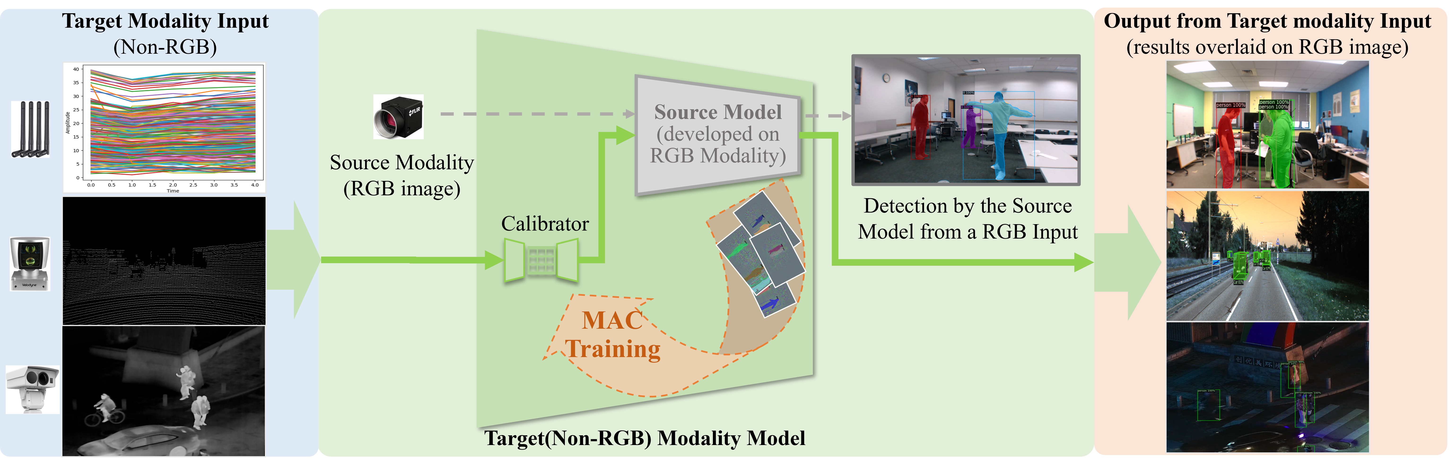
Figure 1: We propose ModAlity Calibration (MAC) for switching input modalities of DNN models. Our “Target Modality Model" is constructed and trained upon a pre-trained source-modality (RGB-input) model by “MAC Training". The dashed arrows “$\mathbf{\dashrightarrow}$" are for training only. In inference, each target-modality(Non-RGB) input is processed along the thick solid green arrows “→".

Although research on the DNN-based perception problem has been largely focused on RGB-input models, there are wide scenarios in that non-RGB sensors have clear advantages over RGB cameras. For instance, wireless signals Zhao et al. (2018); Wang et al. (2019a) can easily penetrate furniture occlusion and identify human bodies for their Dielectric properties, while being lighting-free, occlusion-resistant, and privacy-friendly compared to cameras. Lidar scans Geiger et al. (2012); Sun et al. (2020) contain depth information, enabling more accurate and robust object localization than RGB under low light or bad weather. Thermal InfRared(TIR) cameras Hwang et al. (2015); Jia et al. (2021) capture near-infrared ($0.75$-$1.3\mu m$) or long-wavelength infrared ($7.5$-$13\mu m$) signals, which makes, in particular, human bodies more visible than in RGB images and more robust to the visible spectrum interference.

Thanks to the decade of work on RGB-input DNN models, researchers has accumulated extensive resources on image-appeal architectures(e.g., MaskRCNN He et al. (2017), Yolo5 Jocher et al. (2020), Swin-Transformer Liu et al. (2021)), pre-train-datasets (ImageNet Deng et al. (2009), MS-COCO Lin et al. (2014), OpenImages Kuznetsova et al. (2020)), pre-train weights, training tricks He et al. (2018); Zhang et al. (2019); Ghiasi et al. (2020) and code repos(e.g., Detectron2 Wu et al. (2019), mmDetectionChen et al. (2019)). Unfortunately, non-RGB-input models cannot be directly built upon above RGB resources. Instead, one usually needs new DNN designsQi et al. (2017); Zhao et al. (2018); Wang et al. (2019a), from-scratch training, and new data collection/annotation of non-RGB sensors at the comparable scale of RGB databases above.

In this paper, we propose ModAlity Calibration (MAC) for calibrating target-modality inputs to a DNN model developed on the source modality. Figure 1 shows the main idea of MAC. Ahead of a source-modality model, we add a small target-modality-input calibrator module, composing a [Calibrator$|$Source]-structured target-modality model. The calibrator transforms a target-modality input into a source-modality-like tensor highlighting the foreground, which is then mapped to object detection results by the source module. Trained on {source, target} input pairs of zero manual annotation, the MAC target-modality models reach comparable or better metrics on WiFi, Lidar, and Thermal Infrared than the baselines that require 100% manual annotation. This is achieved by our MAC training techniques that learn prior knowledge from the enclosed source module and iteratively regularize gradients on the calibrator layers. MAC training helps the detection task by mimicking the foreground features of the source modality inputs.

Summary of Contributions:

• MAC, A simple pipeline, is proposed for building Non-RGB-input models upon pre-trained RGB-input models in reducing the DNN design efforts and training data.

• MAC training techniques are proposed to address the special vanishing gradient problem arising by adding a calibrator to a pre-trained RGB perception model. MAC training introduces strong and dense gradients that significantly improve the target-modality model metrics and reduce the need for annotations.

• Compared with target-modality-input models, (i.e., WiFi, Lidar, Thermal Infrared) under naive training, the MAC training techniques achieve comparable or better metrics without manual annotation (MAC-self-supervised), and significantly better metrics with manual annotation(MAC-supervised).

2 Realated Works

For conciseness, we only list object detection work on the three Non-RGB target modalities (WiFi, Lidar, and Thermal) involved in our experiments.

Modality-specific Perception. In most two-stage approaches, Non-RGB inputs are converted to RGB images before feeding to an RGB-input model. Researchers of Kato et al. (2021); Kefayati et al. (2020); Drob (2021) only convert Wifi signals to low-resolution ($<160\times 120$) RGB images by over-fitting a few antenna layouts. No codes or data are available. Points2Pix  Milz et al. (2019) translates Lidar points to RGB images with a conditional GAN. The infrared images were re-colored to RGB in  Limmer and Lensch (2019); Rajendran et al. (2019) by image translation  Karras et al. (2020).

In single-stage approaches, the whole model is only designed and trained on a non-RGB modality. Due to the lack of spatial representation, the WiFi-input models are mostly focused on coarse-granularity tasks such as crowd counting  Depatla and Mostofi (2018); Liu et al. (2019a) or single-person activity recognition  Wang et al. (2017a); Li et al. (2019).  Wang et al. (2019a) develop pioneer WiFi-specific DNNs for multi-person segmentation and pose estimation. Lidar-input models are specific to point-clouds representations, such as the Point View  Qi et al. (2016, 2017); Shi et al. (2019), the Bird’s Eye View  Yan et al. (2018); Lang et al. (2019) and the Range View( Meyer et al. (2019); Fan et al. (2021)). The range view is popular for its low quantization error and computational costs. Thermal images are close to RGB spatially, enabling  Hwang et al. (2015); Jia et al. (2021) to train RGB-input models on the TIR inputs.

Unlike existing two-stage approaches, we work on perception tasks that learn foreground representation instead of RGB appearances. By enclosing the pre-train source model in the target model, we simplify the design effort and reduce target-modality annotations of the single-stage approaches.

Domain Adaption. By definition, domain adaptation mainly addresses the shift of data sampling distribution. Modality adaption, on the other hand, mainly addresses the change in the spatial, temporal, and physical nature of the inputs. Nevertheless, some works still consider modality adaption as a special case of domain adaption especially in the case of image-to-image translation Murez et al. (2018); Dou et al. (2018); Pizzati et al. (2020); Musto and Zinelli (2020); Xie et al. (2020); Gal et al. (2021). All these works aim to generate realistic image pixels in new domains.

Our work applies to any non-image modalities such as WiFi signals. Instead of pursuing realistic pixels, we ONLY generate foreground-associated features contributing to the detection tasks, which aims to reduce the efforts in DNN design and data annotation. Moreover, for simplicity, this work is presented under the assumption that the source and target modality data are sampled from the same foreground/background distributions, such that MAC is only focused on reducing the discrepancy between modalities.

Knowledge Distillation between Models. Teacher-to-student Knowledge Distillation (KD) is a popular approach  Hinton et al. (2015); Dhar et al. (2019). The student models mimic the teacher models in predictive probabilities  Hinton et al. (2015); Li and Hoiem (2017), intermediate features Romero et al. (2014); Wang et al. (2019b), or attention maps Zagoruyko and Komodakis (2016); Wang et al. (2017b); Liu et al. (2020); Chen et al. (2017). When the teacher and student models have different input modalities  Gupta et al. (2016), KD requires the same amount of annotated source-target data as those in the teacher training. All KD methods run the teacher and student in parallel during training.

Unlike KD, our [Calibrator$|$Source] target model is initialized and supervised by the enclosed Source module, which requires neither an independent teacher inference dataflow nor fully annotated target-modality data. Ablation study shows that MAC clearly performs better.

Adversarial Training. To improve robustness on imbalanced datasets, many adversarial training strategies explicitly produce hard features/samples: auto-augmentation  Zoph et al. (2020), co-mixup  Kim et al. (2021), random erasing  Zhong et al. (2017), representation self-challenging  Huang et al. (2020a, b), reverse attention  Chen et al. (2020). Regulators such as cross-layer consistency Hou et al. (2019); Wang et al. (2019c) and self-distillation mechanism  Huang et al. (2020c) were also very effective. Generative Adversarial Networks(GAN) implicitly produce hard samples from a discriminator and are recently extended to the object detection tasks by  Rabbi et al. (2020); Liu et al. (2019b).

We improve target model robustness by synthesizing image-like foreground representation and regularising gradients of the enclosed source model.

Vector Quantized Representation. VQ-VAE  van den Oord et al. (2017); Razavi et al. (2019) and VQ-GAN  Esser et al. (2021) show that a quantized latent space provides a compact representation of natural images, language, and audio/video sequence while using a relatively small number of parameters, making them efficient to train and use.

We extend VQVAE to learn the foreground representation shared between modalities.

3 ModAlity Calibration (MAC)

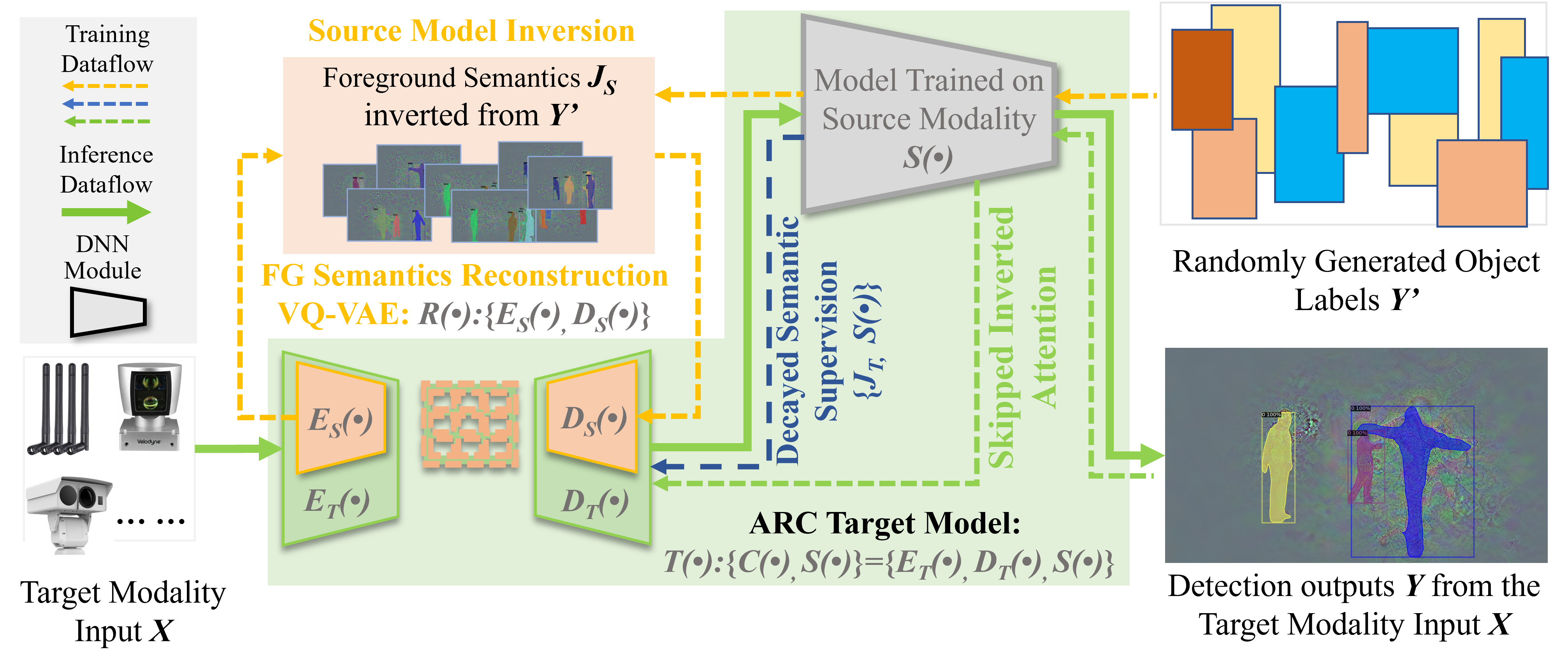
Figure 2: ModAlity Calibration(MAC) Framework. Our MAC target model $T(\cdot):\{E_{T},D_{T},S\}$ is composed of calibrator $C(\cdot):\{E_{T},D_{T}\}$ and source model $S(\cdot)$, with its inference dataflow along the solid green arrows (“$\mathbf{\longrightarrow}$"). The MAC training includes three types of supervision(along the dashed arrows “$\mathbf{\dashleftarrow}$") : (a) Foreground(FG) Semantic Reconstruction(FSR), which leverages the source model prior: the foreground(object) semantics $\mathbf{J}_{S}$ synthesized from $S(\cdot)$ and self-reconstructed by an auxiliary VQ-VAE, $R(\cdot):\{E_{S},D_{T}\}$. (b) Decayed Semantic Supervision(DSS), which regularizes the supervision from precomputed foreground semantics $\mathbf{J}_{T}$ on target modality training data and from source model $S(\cdot)$. (c) Skipped Inverted Attention(SIA), which improves the attention of $C(\cdot)$ output using high-level $S(\cdot)$ layer gradients. See details in the MAC Training section.

Problem Definition: MAC for the object detection task:

• Source model: $S(\cdot):\mathbf{I}\rightarrow\mathbf{Y}$ maps one RGB image $\mathbf{I}\in\Re^{[width\times height\times 3]}$ to the object locations and categories $\mathbf{Y}=[object\_bboxes,object\_mask,object\_class]$.

• Target model: $T(\cdot):\mathbf{X}\rightarrow\mathbf{Y}$ maps one target modality tensor $\mathbf{X}\in\Re^{[width\_T\times height\_T\times channel\_T]}$ to $\mathbf{Y}$.

• MAC target model: $T(\cdot):\{C(\cdot)|S(\cdot)\}$, where the “Calibrator" module $C(\cdot):\mathbf{X}\rightarrow\mathbf{J}$ produces an image-like tensor $\mathbf{J}\in\Re^{[width\times height\times 3]}$. The “Source" module $S(\cdot)$ maps $\mathbf{J}$ to $\mathbf{Y}$.

The goal of MAC is to train a MAC target model $\{C(\cdot)|S(\cdot)\}$ given a pre-trained source model $S(\cdot)$ and a set of $\{\mathbf{X},\mathbf{I}\}$ pairs. (See the framework in Figure 2).

For simplicity, we assume that the source and target modality data are sampled from the same $\mathbf{Y}$ (foreground/background) distributions, such that MAC is only focused on reducing the discrepancy between modalities.

3.1 Reasoning for the $\{C(\cdot)|S(\cdot)\}$ Target Model

If we follow the development procedure of $S(\cdot)$ to develop a new $T(\cdot)$, we need a modality-specific multi-resolution feature extractor (comparable to ResNet), which is coupled with a task-specific output head (Such as the anchor-based or transformer-based bounding box regressors) by multi-resolution skip connections. One also needs annotated $\{\mathbf{X},\mathbf{Y}\}$ data comparable to the amount of the $\{\mathbf{I},\mathbf{Y}\}$ data used in the source model $S(\cdot)$ training.

Under MAC(Figure 2), we only design calibrator $C(\cdot)$ that produces a single-resolution tensor $\mathbf{J}$ feeding to the source module $S(\cdot)$ enclosed in $T(\cdot)$.

Foreground encoding in $C(\cdot)$: Since it is $S(\cdot)$’s expertise to locate and classify objects, $C(\cdot)$ only needs to pass to $S(\cdot)$ some foreground-sensitive features $\mathbf{J}$, i.e., the edges/textures highlighting all the object categories. To generate such foreground features, we revisit the insight of the image-wise Class Activation Maps  Zhou et al. (2016): all pixels of each object category can be mapped to an element of a probability vector by Softmax activation, which highlights foreground pixels assuming category-wise features follow a multi-modal distribution. In order to preserve the internal spatial layout of objects, we encode pixel patches(object parts) under the multi-modal distribution. This is done by a encoder-decoder structure $C(\cdot):\{E_{T},D_{T}\}$ with a quantized latent space inspired by VQ-VAEvan den Oord et al. (2017) (see Figure 2). We set the latent space tensor size to $[width/8,height/8,channel]$, in which every $[1\times 1\times channel]$ vector is hard-coded to one of the multi-modal centers of local patches, denoted as codebook $\{B_{i}\in\Re^{1\times 1\times channel}\}|_{i=1,\dots,p}$. Mapping such a VQ-VAE-like latent space to image-like feature $\mathbf{J}$, the calibrator decoder $D_{T}$ simply takes the same structure as the standard VQ-VAE decoder. The calibrator encoders $E_{T}$ for target-modality inputs are similar to the standard VQ-VAE encoder with minor adjustments below.

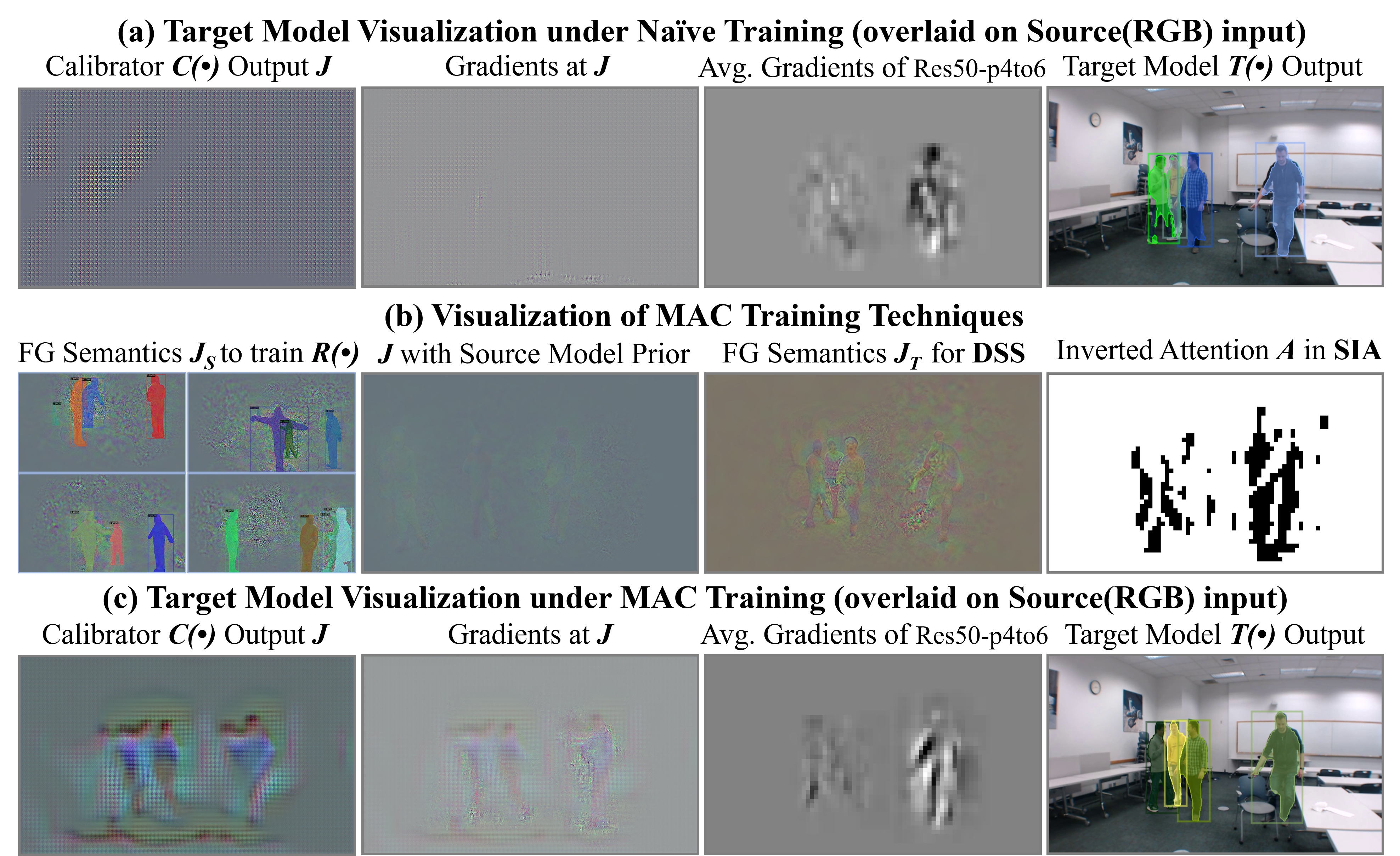
Figure 3: Training strategy examples on a WiFi-input target model $T(\cdot):\{C(\cdot),S(\cdot)\}$. Here, the source model $S(\cdot)$ is an RGB-input ResNet50-FPN-Mask-RCNN. (a) Target model visualization under Naïve training shows neither foreground-sensitive features in $C(\cdot)$ output $\mathbf{J}$ nor any clear gradients at $\mathbf{J}$ compared to “Avg. Gradients of Res50-p4to6" (the high-level gradients visualized by resizing and averaging on one channel). (b) Visualization of MAC training techniques (described the MAC Training section). (c) Target model visualization under MAC training shows clear foreground-sensitive features, strong gradients at $\mathbf{J}$ and better detection. Note that, in “Target Model $\mathbf{T}(\cdot)$ Output" of the 3rd row, all persons are detected with better masks than “Target Model $\mathbf{T}(\cdot)$ Output" of the 1st row. Please zoom in to see all the instance masks.

Target-Modality Encoder $E_{T}$: The WiFi signal corresponding to one synchronized RGB image  Wang et al. (2019a), is represented as the Channel State Information (CSI)  Halperin et al. (2011) tensor [samples, transmitters, receivers, sub-carriers]. The CSI tensor elements has no spatial dependence as RGB pixels. In this case, we construct $E_{T}$ by adding Wi2Vi  Kefayati et al. (2020) layers in front of a VQ-VAE encoder. For other target modalities (infrared and Lidar range images) that have the image-like tensor shape, we directly use the VQ-VAE encoder structure for $E_{T}$.

Remarks: To enable $T(\cdot):\{C(\cdot),S(\cdot)\}$ to produce the same $\mathbf{Y}$ as that of a pre-trained source model $S(\cdot)$, the latent space of $C(\cdot)$ has to contain the same semantics as those encoded in $S(\cdot)$. This opens the possibility to learn $C(\cdot)$ from $S(\cdot)$, without requiring a huge set of $\{\mathbf{X},\mathbf{Y}\}$ training data.

3.2 MAC Training

The devil lies in the training of the MAC target model $T(\cdot)$. There are two naïve sources of supervision: (1) Given the $\{\mathbf{X},\mathbf{I}\}$ pairs, one may pre-train $C(\cdot)$ to approximate $\mathbf{I}$. Since there are usually more background pixels than foreground pixels, the pre-trained $C(\cdot)$ outputs $\mathbf{J}$ may largely be background textures that are irrelevant to the detection tasks. (2) Given abundant $\{\mathbf{X},\mathbf{Y}\}$ training pairs, one may randomly initialize $C(\cdot)$ and update all $T(\cdot)$ layers using the gradients back-propagated from the source model losses. Such a strategy suffers from the vanishing gradient problem  Bengio et al. (1994); Glorot and Bengio (2010) and is contradictory to the common DNN training practice (for instance, ImageNet-pretrained Resnet + randomly initialized Mask-RCNN). In fact, the randomly initialized $C(\cdot)$ should receive the strong gradients for updating, while the pre-trained weights of $S(\cdot)$ should be preserved by updating with weak gradients. Figure 3(a) shows that the naïve training produces neither foreground-sensitive features nor any clear gradients at $\mathbf{J}$ comparable to the high-level gradients, e.g., “Avg. Gradients of Res50-p4to6".

To address the above issues, we propose the MAC training techniques below (Also see diagram in Figure 2).

Road-map: MAC training techniques address the special vanishing gradient problem arising by adding a calibrator to a pre-trained RGB perception model. Source Model Inversion(SMI) discovers the dense image-like foreground features. Foreground Semantics Reconstruction(FSR) introduces dense image-like supervision by pre-training the calibrator. Decayed Semantic Supervision (DSS) uses $\mathbf{J}_{T}$ to provide strong gradients for foreground supervision, then let the weaker gradients from $\mathcal{L}_{S}$ amend the acute details. Skipped Inverted Attention (SIA) channels the high-level gradient-based attention from $S(\cdot)$ back to the low-level feature layers of $C(\cdot)$. Along with section 3.2, Fig. 3 and Table 4 demonstrate how the gradients are improved by each MAC training technique.

3.2.1 Source Model Inversion(SMI)

We first guide the calibrator $C(\cdot)$ to produce foreground-sensitive features leveraging a pre-trained source model $S(\cdot)$. Given the pre-trained $S(\cdot)$ and the object annotation $\mathbf{Y}$, we conduct model inversion  Vondrick et al. (2013); Cao and Johnson (2021) to generate $\mathbf{J}_{S}$ by minimizing the $S(\cdot)$ losses,

$$\mathcal{L}_{S}(S(\mathbf{J}_{S}),\mathbf{Y})=\lambda_{bbox}\mathcal{L}_{bbox}+\lambda_{cls}\mathcal{L}_{cls}+\lambda_{mask}\mathcal{L}_{mask}.$$ (1)

This problem is solved by image-wise optimization: freezing all the $S(\cdot)$ layers, computing gradient from $\mathcal{L}_{S}(\mathbf{J}_{S},\mathbf{Y})$ and only updating $\mathbf{J}_{S}$ from its random initialization. After the optimization converges, $\mathbf{J}_{S}$ is synthesized as a most probable and style-invariant “image" from which $S(\cdot)$ can detect $\mathbf{Y}$. $\mathbf{J}_{S}$ only captures the edge-like patterns of the foreground (See pixels marked in colors Figure 3(b)). We call $\mathbf{J}_{S}$ the Foreground Semantics.

Compared with the original RGB pixels, we see $\mathbf{J}_{S}$ a clean foreground-focused supervision to guide $C(\cdot)$ training. Compared with the small gradient amplitude from $\mathcal{L}_{S}$, the amplitude of $\mathbf{J}_{S}$ is comparable to $\mathbf{I}$ resulting in strong gradients on the $C(\cdot)$ layers.

To increase the diversity of $\mathbf{J}_{S}$, we also randomly generate the object layouts in $\mathbf{Y}^{\prime}$ of different bbox locations (instance masks for Mask-RCNN) and class labels. The random object labels $\mathbf{Y}$ introduce diverse object locations, sizes, and co-occurrences. In addition, the noise diversity of the foreground is also introduced by the random $\mathbf{J}$ initialization of model inversion from different $\mathbf{Y}^{\prime}$s.

3.2.2 Foreground Semantics Reconstruction(FSR)

Next, to inject the prior knowledge in $J_{S}$ to calibrator $C(\cdot)$, we train an auxiliary VQ-VAE, $R(\cdot)=\{E_{S},D_{S}\}:\mathbf{J}_{S}\rightarrow\mathbf{J}_{S}$ that encodes and reconstructs $J_{S}$. Then we share the $R(\cdot)$’s VQ codebook with $C(\cdot)$, and initialize the $C(\cdot)$’s decoder $D_{T}(\cdot)$ by the $R(\cdot)$’s decoder $D_{S}(\cdot)$ weights. We call the initialization method of $C(\cdot)$ as Foreground Semantics Reconstruction(FSR).

In addition, our target model $T(\cdot)$ encloses $S(\cdot)$ as a module, which can explicitly inherit the source model knowledge by initializing it with the pre-trained source model weights.

Finally, to accommodate both above priors incorporated into $C(\cdot)$ and $S(\cdot)$, we train $T(\cdot)$ in a two-stage update strategy: (i) fix $S(\cdot)$ and only update $C(\cdot)$ until it converges; (ii) continue training by updating both $C(\cdot)$ and $S(\cdot)$.

Remarks: (i) $\mathbf{J}_{S}$ is synthesized from a pre-trained source model over synthetic $\mathbf{Y}^{\prime}$. No manually annotated source inputs $\mathbf{I}$ are needed. (ii) Given that the $R(\cdot)$ training requires no annotation on $\mathbf{X}$, and the $S(\cdot)$ module can provide pseudo ground truth $\mathbf{Y}_{pseudo}$ for the $\{\mathbf{X},\mathbf{I}\}$ pairs, the overall training of $T(\cdot)$ is self-supervised (zero manual annotation on $\mathbf{X}$).

3.2.3 Decayed Semantic Supervision (DSS)

The Decayed Semantic Supervision is used to regularize $\mathcal{L}_{S}$ gradients with image-space semantic supervision. Given a pre-trained $S(\cdot)$ and either $\{\mathbf{X},\mathbf{Y}_{pseudo}\}$ (the self-supervised MAC) or $\{\mathbf{X},\mathbf{Y}\}$ (the supervised MAC) as the target model training data, we invert $S(\cdot)$ to generated $\mathbf{J}_{T}$ as GT to directly supervise $C(\cdot)$. The $C(\cdot)$ output $\mathbf{J}$ is an image-like tensor, therefore $C(\cdot)$ can be trained with image-based losses against $J_{T}$ along with the source loss $\mathcal{L}_{S}$, leading to the Semantic Supervision (SS) loss,

$$\mathcal{L}_{SS}(\mathbf{J},\mathbf{J}_{T})=SSIM(\mathbf{J},\mathbf{J}_{T})+L_{1}(\mathbf{J},\mathbf{J}_{T})+\mathcal{L}_{S},$$ (2)

where $SSIM(\cdot,\cdot)$ is the structural similarity loss and $L_{1}(\cdot,\cdot)$ is the L1-norm loss (Both losses provide higher amplitudes gradients than gradients back-propagated from $\mathcal{L}_{S}$). Due to the image-wise optimization nature of model inversion, each $\mathbf{J}_{T}$ over-fit different noise of the source model $S(\cdot)$. When training on all $\mathbf{J}_{T}$ samples, $C(\cdot)$ tends to produce averaged foreground semantics smoothing out sample-specific details that may be critical to detection.

We propose a simple fix, called Decayed Semantic Supervision(DSS), to such a problem:

$$\mathcal{L}_{DSS}=\lambda_{DSS}(SSIM(\mathbf{J},\mathbf{J}_{T})+L_{1}(\mathbf{J},\mathbf{J}_{T}))+\mathcal{L}_{S},$$ (3)

where $\lambda_{DSS}$ is a scalar that continuously decays with the increase of iterations (see supplementary materials).

How DSS works? The foreground semantics $\mathbf{J}_{T}$ only contain relatively clean foreground features reconstructed from $\mathbf{Y}$, but the background features are random due to the image-wise optimization of SMI. When training over all the data, using $\mathbf{J}_{T}$ throughout all training iterations will contaminate the target model with random background noise. By smoothly decaying lambda_DSS, $\mathbf{J}_{T}$ provides strong gradients/supervision on foreground features in the early iterations, then the gradients from the source model losses $\mathcal{L}_{S}$ amend the acute overall details in later iterations. The effectiveness of DSS is qualitatively shown in Figure 3(b) and quantitatively evaluated in Table 4.

3.2.4 Skipped Inverted Attention (SIA)

The Skipped Inverted Attention (SIA) is applied to amplify and balance the gradients from $\mathcal{L}_{S}$. The strong gradients at the high-level layers of $S(\cdot)$ (see “Avg. Gradients of Res50-p4to6 " in Figure 3(a) of a ResNet-FPN-MaskRCNN $S(\cdot)$ module) does not propagate into strong “Gradients at $\mathbf{J}$".

To address this issue, we generate a 2D inverted attention mask $\mathbf{A}$ from the above gradients $\mathbf{G}$ and skip the earlier ResNet layers backward to supervise $C(\cdot)$. Formally, from $\mathbf{G}\in\Re^{width\times height\times channel}$, $\mathbf{A}(\mathbf{G})\in\Re^{width\times height}$ is computed as,

$$\mathbf{a}(i)=\cases{0},\quad\textnormal{if}\quad\sum_{j=1}^{channel}g(i,j)\geq q\\ 1,\quad\textnormal{otherwise}$$ (4)

where $g_{p}$ is a scalar of the $(100-p)$^th percentile of $\sum_{j=1}^{channel}\mathbf{G}(:,j)$, ($i\in[1,\cdots,width\times height]$). Low $\mathbf{G}$ and high $\mathbf{A}$ values denote under-represented regions by $S(\cdot)$ marked by white pixels in Figure 3(b)“Inverted Attention $\mathbf{A}$ in SIA". Forwarding the element-wise masked feature $\mathbf{A}\odot\mathbf{J}$ through $S(\cdot)$, $T(\cdot)$ is updated by the SIA loss

$$\mathcal{L}_{SIA}=\mathcal{L}_{S}(S(\mathbf{A}\odot\mathbf{J}),\mathbf{Y}).$$ (5)

Training with the $\mathbf{A}\odot\mathbf{J}$-induced loss $\mathcal{L}_{SIA}$, $C(\cdot)$ is forced to balance feature learning in all regions (See the strong foreground gradients at $\mathbf{J}$ in Figure 3(c)).

In summary, the MAC Training procedure consists of initializing $T(\cdot)$ with (1) and updating $T(\cdot)$ with (2-3). Figure 3(c) shows that MAC training produces foreground-focused features in $\mathbf{J}$, stronger gradients at $\mathbf{J}$, and better instance mask detection than the Naïve training in Figure 3(a).

4 Experiments

We use the following keywords throughout this section. “Standard" refers to the source model training strategy (backbone pretrained on Imagenet and $S(\cdot)$ fully updated with $\mathcal{L}_{S}$). “MAC training" refers to our techniques. “MAC-Self-supervised": Training on Pseudo-GT generated by inference $S(\cdot)$ with the source inputs of the target-source pairs in the target-modality training set. “MAC-Supervised": Training on manually annotated GT of the target-modality training set. “MAC-Semi-Supervised": Training on Pseudo-GT and a subset of manually annotated GT. All implementation details are described in the supplementary materials.

Model (on x101-GT)	Input	Training Strategy	Box	Mask	Target-Modality	Inference
			mAP $\uparrow$	mAP $\uparrow$	Annot. $(\%)\downarrow$	Flops$|$#Para.
Source models $S(\cdot)$
R50-FPN-MaskRCNN	RGB	Coco-pretrain Wu et al. (2019) + Standard	82.36	87.94	-	61.42G$|$44.30M
Target models baselines
PiW Wang et al. (2019a)$|S(\cdot)$	CSI	Source Init. $S(\cdot)$+ Standard	59.86	45.08	100	62.27G$|$45.0M
Wi2Vi Kefayati et al. (2020)$|S(\cdot)$	CSI	RGB-FG-pretrained Wi2Vi Kefayati et al. (2020)	0.12	0.09	100	63.22G$|$49.82M
Wi2Vi Kefayati et al. (2020)$|S(\cdot)$	CSI	Source Init. $S(\cdot)$+Standard	68.12	54.79	100	63.22G$|$49.82M
Ours target models $C(\cdot)|S(\cdot)$
MAC-Self-supervised	CSI	MAC training	71.21	63.67	0	70.10G$|$51.34M
MAC-Semi-Supervised	CSI	MAC training	74.65	65.86	10	70.10G$|$51.34M
MAC-Supervised	CSI	MAC training	77.38	66.49	100	70.10G$|$51.34M

Table 1: WiFi CSI-input model results on the Person-in-Wifi(PiW) dataset (all $16$ layouts). All models were trained and evaluated against GTs generated by X101-FPN-MaskRCNN($\times 3$) in Detectron2 model zoo. The best target model metrics are in bold.

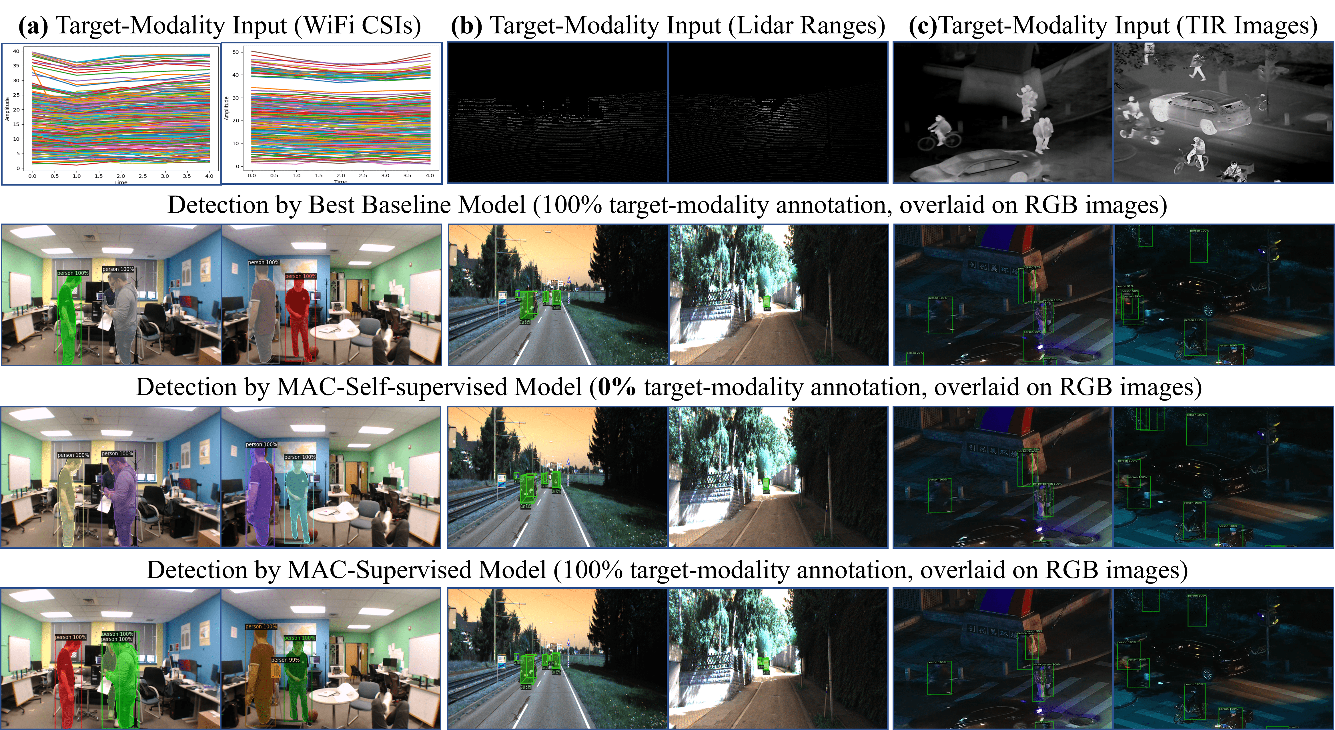
Figure 4: Qualitative results on three target-modality inputs (a) WiFi CSIs (amplitude sequences corresponding to each frame), (b) Lidar Ranges (sparse depth points projected on the pixel grid) and (c) Thermal InFraRed (TIR) images.

4.1 WiFi-input Target Model

In Table 1, we build WiFi-input models upon an RGB-input MaskRCNN model(source model) on the Person-in-Wifi(PiW) Wang et al. (2019a) dataset. The PiW dataset contains synchronized RGB videos (20FPS) and Channel State Information(CSI) sequences (100Hz) of the Wifi signal. There are 16 indoor layouts 16 with multiple persons captured. One RGB frame (resized to $[3,640,384]$) corresponds to a CSI tensor ([CSI_samples, transmitters, receivers, sub-carriers]=$[5,3,3,30]$). The model in Wang et al. (2019a) only produces image-wise semantic mask and body-joint heatmaps and cannot be directly compared on person detection metrics. No common ground truth was annotated to compare the RGB-input model and WiFi-input model.

To overcome these drawbacks, we propose the following setting: (1) All models are trained on and evaluated against a common ground truth X101-GT, which is generated by an MS-COCO-pre-trained ResNeXt101-FPN-MaskRCNN-32x8d(x3) model in Detectron2 Wu et al. (2019) on RGB inputs. (2) Source model $S(\cdot)$: an RGB-input R50-FPN-MaskRCNN pre-trained on MS-COCO and fine-tuned on the PiW data. (3) Target model baseline (“PiW$|S(\cdot)$" and “Wi2Vi$|S(\cdot)$"): composed by adding the CSI-to-RGB modules of PiW Wang et al. (2019a) and Wi2Vi Kefayati et al. (2020) to $S(\cdot)$ respectively. We train the target baselines by randomly initializing their CSI-to-RGB modules, initializing $S(\cdot)$ with source model weights, and training with the “Standard" strategy. Pre-training the Wi2Vi module to synthesize the foreground-cropped images Kefayati et al. (2020), denoted by “RGB-FG-pre-trained WiVi", does not work well on the multi-person and multi-layout PiW data.

“Our target models $C(\cdot)|S(\cdot)$" were trained by “MAC" under three configurations: “MAC-Self-supervised" produces box and mask mAP of [$71.21,63.67$] using 0% target-modality annotation, which outperforms the best target baseline metrics [$68.12,54,79$] on 100% target-modality annotation. This shows that MAC effectively transferred priors from the strong RGB-input model to the CSI-input model. Compared to the best baseline(Wi2Vi), the overheads of MAC models are 10% in Flops and 3% in #Para. “MAC-Semi-supervised" and “MAC-Supervised" outperforms all other target models using $10$% and 100% target-modality annotation, respectively. Figure 4(a) visualizes the results.

Models	Input	Training	Car BEV AP$|_{40}$	Car 3D-Bbox AP$|_{40}$	Target-Modality	Inference
			[Easy, Med., Hard] $\uparrow$	[Easy, Med., Hard] $\uparrow$	Annot. $(\%)\downarrow$	Flops$|$#Para.
Source models $S(\cdot)$
DD3D-DLA34 Park et al. (2021)(github)	RGB	Standard	[31.7, 24.4, 21.7]	[22.6, 17.0, 14.9]	-	109.9G$|$25.6M
Target model baselines
DD3D-DLA34	Range	Standard	[40.7, 25.4, 22.0]	[29.4, 17.9, 14.9]	$100$	109.9G$|$25.6M
Ours target models $C(\cdot)|S(\cdot)$
MAC-Self-supervised	Range	MAC	[41.5, 26.1, 23.2]	[30.2, 18.2, 15.4]	0	123.6G$|$28.1M
MAC-Semi-Supervised	Range	MAC	[43.6, 27.3, 25.5]	[32.1, 19.8, 16.8]	10	123.6G$|$28.1M
MAC-Supervised	Range	MAC	[46.3, 33.4, 30.9]	[35.4, 21.8, 19.9]	$100$	123.6G$|$28.1M

Table 2: Lidar Range-input model results on the KITTI validation set. Metrics (Car metrics only) are evaluated on the frontal sector of Lidar scans matching the RGB Camera 2 field-of-view. The best target model metrics are in bold.

4.2 Lidar-input Target Model

We build Lidar Range-input models upon an RGB-input DD3D model Park et al. (2021) on the Kitti-3D dataset Geiger et al. (2012). Since there is no $360$-degree RGB coverage that matches the 360-degree Lidar scans, we only evaluate results on the frontal-view sector of the Lidar scans overlapped the RGB Camera#2 field-of-view. The 32-beam Lidar scans at 1-degree horizontal resolution, creating $32\times 90$ points in the frontal-view sector, which are then projected to the $384\times 1270$ pixel grid to match the RGB pixels. Following Fan et al. (2021); Meyer et al. (2019), the missing range pixels are filled by a fixed depth value of $80$ (meters). Following Park et al. (2021), we report AP$|_{40}$ Simonelli et al. (2020) computed on the training$|$testing split of $3712|3769$ samples. As shown in Figure 4(b), the range image has very sparse depth pixels with no visual appearance.

In Table 2, the “Target model baseline", directly training a DD3D on Range-inputs, produces higher metrics than the RGB-input Source models, which indicates the advantage of the Lidar over the RGB camera. It appears that the weak RGB-input model cannot provide good prior knowledge to develop the Lidar-input model. However, the MAC-Self-supervised target model, with 0% target-modality annotation, still outperforms the target baseline trained on 100% annotation. Trained on 10% and 100% target-modality annotations respectively, our MAC-Self-Supervised and MAC-Supervised target models easily outperform all other models in all AP$|_{40}$ metrics. Figure 4(b) visualizes the results.

4.3 Infrared-input Target Model

On the LLVIP dataset Jia et al. (2021) , we show how MAC works when the source modality(RGB) contains far less information than the target modality(Thermal InfRared (TIR)) under low-light vision. We used the official training/testing split containing 15488 RGB-TIR pairs with manually labeled 2D bounding boxes.

In Table 3, we used the R50-FPN-FastRCNN (input size 1024$\times$1280) for both the source model (RGB input) and target model baseline (TIR input). Both models were pre-trained on MS-COCO and fine-tuned on the RGB and TIR inputs respectively. The MAC target models are trained with the MAC training algorithm. The source model produces Bbox Average Precision(Box AP) of $43.83$, which is clearly inferior to the target model baseline (Box AP $55.58$), therefore may not provide strong priors or correct Pseudo labels for the target model. However, the MAC-Self-supervised target model still gets Box AP of $55.63$ using 0% target-modality annotation, which is comparable to the target baseline trained on 100% annotation. With only 10% annotation, the MAC-Semi-supervised model easily outperforms the target baseline. With 100% annotation, the MAC-supervised target model outperforms all other models. Figure 4(c) visualizes the results. In this experiment, the higher MAC overheads are due to the large input size, which could be reduced by concatenating $C(\cdot)$ with the smaller feature maps of $S(\cdot)$.

Models	Input	Training	Box	Target-Modality	Inference
			AP $\uparrow$	Annot. $(\%)\downarrow$	Flops$|$#Para.
Source model $S(\cdot)$
R50-FPN-FasterRCNN	RGB	Standard	43.83	-	255G$|$41.70M
Target model baseline
R50-FPN-FasterRCNN	TIR	Standard	55.58	$100$	255G$|$41.70M
Ours target models $C(\cdot)|S(\cdot)$
MAC-Self-supervised	TIR	MAC	55.63	0	302G$|$44.35M
MAC-Semi-Supervised	TIR	MAC	57.08	$10$	302G$|$44.35M
MAC-Supervised	TIR	MAC	58.05	$100$	302G$|$44.35M

Table 3: Thermal InfRared TIR-input model results on the LLVIP dataset. Best in bold.

4.4 Ablation Study

In Table 4, we conduct an ablation study of the MAC training techniques on the “2018_10_17_2" subset of the PiW dataset. We start with the baseline training strategy: “RandInit+$\mathcal{L}_{S}$", and add MAC or alternative techniques in four groups. The cumulative relation among groups is denoted by their indents of “$+$"s. Each group is added upon its previous MAC techniques. For instance, “Feature-based KD…" and “Source Init. $S(\cdot)$…" are both added upon “FSR pretrained $C(\cdot)$…".

Training Strategies on $C(\cdot)|S(\cdot)$	Box	Mask	Target-Modality
	AP $\uparrow$	AP $\uparrow$	Annot. (%)$\downarrow$
Rand. Init.+Standard (Baseline)	75.28	66.26	$100$
MAC (bold rows) vs. Alternative techniques
+ w/o FSR-pretrained $C(\cdot)$	76.69	67,03	$100$
+ FSR-pretrained $C(\cdot)$	78.83	68.73	$100$
+ Feature-based KD Zhang and Ma (2021) from $S(\cdot)$	70.90	54.43	$100$
+ Source Init. $S(\cdot)$ and two-stage update	80.36	70.55	$100$
+ SS loss $\mathcal{L}_{SS}$ (Eq.(2))	81.03	71.09	$100$
+ DSS loss $\mathcal{L}_{DSS}$ (Eq.(3))	81.60	71.62	$100$
+ RSC Huang et al. (2020b) on the $C(\cdot)$ output layer	80.94	71.21	$100$
+ RSC Huang et al. (2020b) on the Res-50-p5 layer	81.89	71.92	$100$
+ SIA(Eq.(5)	82.15	72.33	$100$
MAC-Self-supervised	75.14	65.96	0

Table 4: Ablation study of training techniques on MAC target model $C(\cdot)|S(\cdot)$ on the “2018_10_17_2" subset of PiW. The cumulative relation among groups of “MAC vs.Alternative techniques" are denoted by their indents of “$+$"s. Each group of techniques is added upon the MAC techniques (bold rows) of the previous group.

Within each compared group, the MAC technique (bold rows) produces better metrics than their alternative counterparts. “FSR-pretrained $C(\cdot)$" and “Source Init. $S(\cdot)$ and two-stage update" provide better priors to the target model than“w/o FSR" and “Feature-based KD". SIA is better than RSC Huang et al. (2020b) which computes and applies attention on the same layer (“the C(·) output layer" or “the Res-50-p5 layer"). Using 100% target-modality annotation, our final model (after applying SIA) produces [82.15, 72.33], which is significantly better than the baseline ([75.28, 66.26]). Trained on the Pseudo GT generated by $S(\cdot)$, MAC-Self-supervised produces [75.14, 65.96] comparable to the baseline that is trained on $100\%$ manual target-modality annotation. Besides using the same number of pseudo images as the real images, we also tried fewer (0, 1/2) pseudo images and got [77.13,68.25] and [79.83,70.12] respectively. We also tried vanilla VAE as a calibrator and only got [0.5, 0.3] due to the VAE’s inferior fine-grain reconstruction ability than VQVAE.

In summary, DSS is proven better than SS, and also improves upon “Source Init. S(·) and two-stage update". SIA is proven better than two RSC variants, and also improves upon “DSS loss LDSS (Eq.(3))". “MAC-Self-supervised", that uses 0 manual annotations, has comparable performance as “Baseline" that uses 100% manual annotations. Using 100% annotations, “MAC-Supervised" is significantly better than “Baseline".

5 Discussion

Modality Calibration vs. Domain Adaption: By definition, domain adaptation mainly addresses the shift of data sampling distribution. Our modality calibration problem mainly addresses the change in the spatial, temporal, and physical nature of the inputs. Although some work consider image translation as both modality calibration and domain adaption, our work applies to any non-image modalities such as WiFi signals. Instead of pursuing realistic pixels in image domain, we ONLY generate foreground-associated features contributing to the detection tasks, which aims to reduce the efforts in DNN design and data annotation. Moreover, for simplicity, this work is presented under the assumption that the source and target modality data are sampled from the same foreground/background distributions, such that MAC is only focused on reducing the discrepancy between modalities.

Pros. and Cons. of MAC: By adding a calibrator to a pre-trained RGB perception model, MAC introduces an efficient pipeline for switching input modalities of DNNs, while bringing back the old deep learning challenge: the vanishing gradient problem  Bengio et al. (1994); Glorot and Bengio (2010). To address this challenge, multiple MAC training techniques, FSR, DSS, and SIA, are developed to generate strong and dense gradients.

MAC-Self-supervised vs. MAC-Supervised: In “MAC-Self-supervised" (see the cases of “Target-Modality Annot." $0\%$ in Table 1-4) the GTs for training the MAC target model are the pseudo annotations produced by inferencing a pre-trained source model. There is NO manual GT for the target modality. “MAC-Supervised" uses the real manually annotated GTs (see the case of “MAC-Supervised" with “Target-Modality Annot." $100\%$ in Table 1-4). This presents us with options to balance the performance and the effort of annual data annotation.

General use of MAC: The same FSR, DDS, and SIA training techniques can be used to develop all non-RGB modality models. Only different calibrators need to be developed for different non-RGB modalities.

6 Conclusions

We proposed MAC, an efficient pipeline for switching input modalities of DNNs. In training a target-modality model, MAC leverages the prior knowledge from the source-modality model and requires as few as zero target-modality annotations. The MAC components (FSR, DSS, SIA) could potentially be used to compose any cross-modality models, for instance, using DALL-E-mini as a calibrator to compose a text-input model.

Potential negative social impact: If the source model were trained on private RGB images, data-privacy concerns may arise from the source model inversion operation in MAC.

Appendix

Implementation Details

WiFi-input Model For the WiFi-input model, we use R50-FPN-MaskRCNN He et al. (2017) as our source model, and Wi2Vi Kefayati et al. (2020) + VQ-VAE2 Razavi et al. (2019) as calibrator. We used two-level latent maps which are approximately 16x, 2x times smaller than the original image. The codebook size is set as 1024. The decay factor for Decayed Semantic Supervision $\lambda_{DSS}$ is set as 0.9999. The percentile threshold $p$ used in Skipped Inverted Attention is 0.1.

We use 8 GPUs with batch size 64 for training. Following the R50-FPN-MaskRCNN training codes, the MAC target-input model is trained using the Adam optimizer for 150k iterations with a weight decay of 0.0001 and an initial learning rate of 0.0001. The training process is warmed up by a linear warm-up-scheduler with 0.001 factor for 1k iterations and then the learning rate is decayed by 10x times at 90k iterations.

Lidar-input Model For the Lidar-input model, we use DD3D Park et al. (2021) as our source model and VQVAE2 as calibrator. We used three-level latent maps which are approximately 32x, 4x, 2x, times smaller than the original image. The codebook size is set as 4096. We use 8 GPUs with batch size 64 for training. The decay factor for Decayed Semantic Supervision $\lambda_{DSS}$ is set as 0.9995. The percentile threshold $p$ used in Skipped Inverted Attention is 0.1.

Following DD3D training codes, the MAC target-input model is trained using SGD optimizer for 24k iterations with weight decay 0.0001, momentum 0.9, and an initial learning rate of 0.002. The training process is warmed up by a linear warm-up-scheduler with 0.001 factor for 2k iterations and then the learning rate is decayed by 10x times at 21.5k and 25k iterations.

Infrared-input Model For the Infrared-input model, we use R50-FPN-FastRCNN as our source model and VQVAE2 as the calibrator. We used three-level latent maps which are approximately 32x, 4x, 2x, times smaller than the original image respectively. The codebook size is set as 4096. We use 8 GPUs with batch size 64 for training. The decay factor for Decayed Semantic Supervision $\lambda_{DSS}$ is set as 0.9999. The percentile threshold $p$ used in Skipped Inverted Attention is 0.1.

Following the R50-FPN-FastRCNN training codes, the MAC target-input model is trained using Adam optimizer for 50k iterations with a weight decay of 0.0001 and an initial learning rate of 0.0001. The training process is warmed up by a linear warm-up-scheduler with 0.001 factor for 1k iterations and then the learning rate is decayed by 10x times at 30k iterations.

Training/inference Costs Take the setting in the main paper Table 4 for example. Compared to training the [Calibrator|Source] model from scratch (Baseline in Table 4), MAC training introduces three main overheads: pre-computing Foreground Semantics $J$, pretraining $C(\cdot)$ in FSR, and SIA, which respectively cost around 200%, 20%, and 10% of the baseline training time. Note that pre-computing Foreground Semantics $J$ is a one-time data pre-processing stage and does not join the training iteration of the target-modality model. The inference overhead is introduced only by the calibrator over the source model. In the main paper Table 1-3, the calibrators add 14% 13%, and 15% of the source model inference time, respectively.

Source Model Inversion Examples

Our Source Model Inversion(SMI) generate foreground semantics images $\mathbf{J}_{S}$. We show examples of SMI respectively on the three different source models in Figure 5, Figure 6 and Figure 7. In all cases, $\mathbf{J}_{S}$ shows clear foreground-sensitive features.

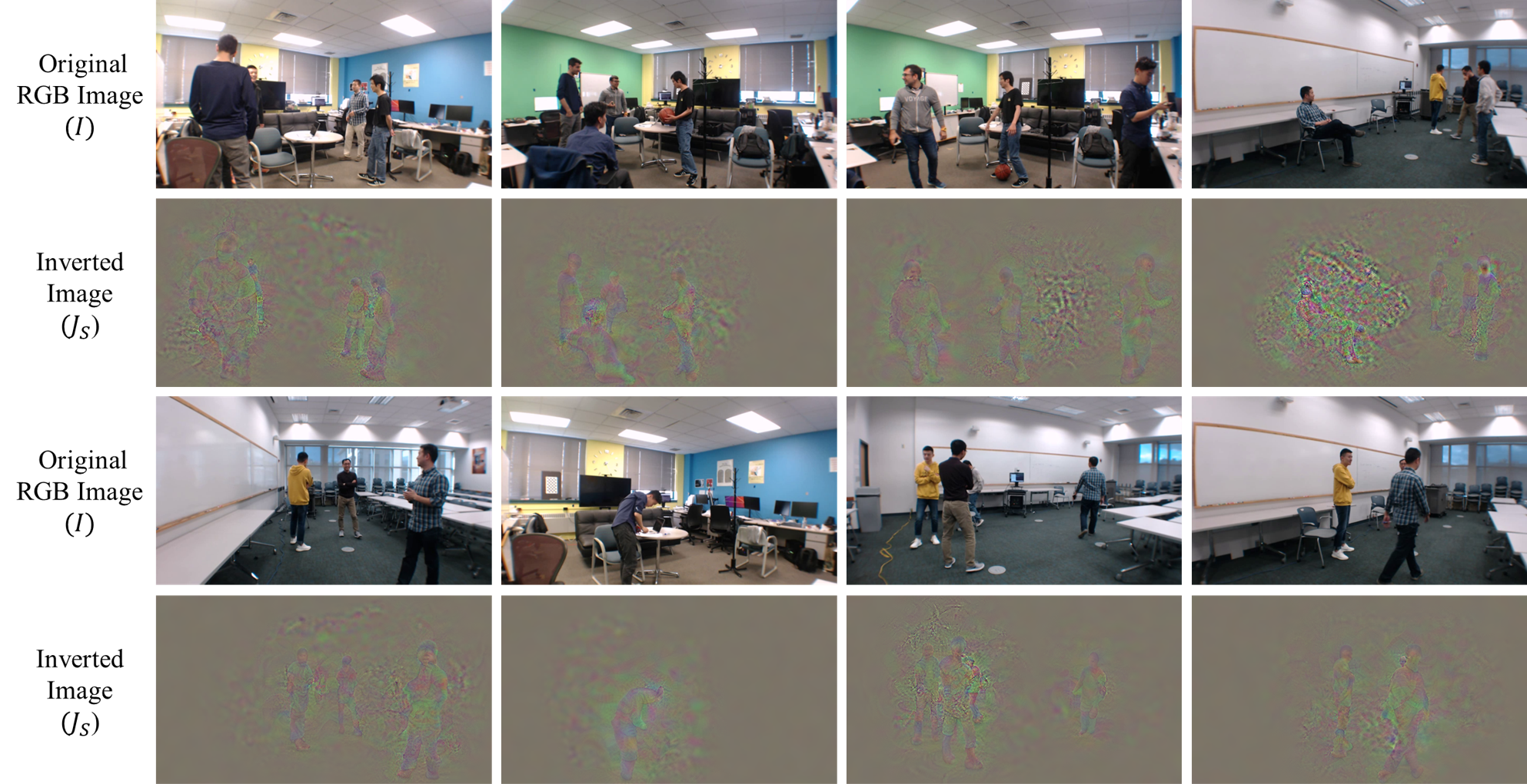
Figure 5: Model inversion examples of the R50-FPN-MaskRCNN source model in the “WiFi-input Target Model" experiments

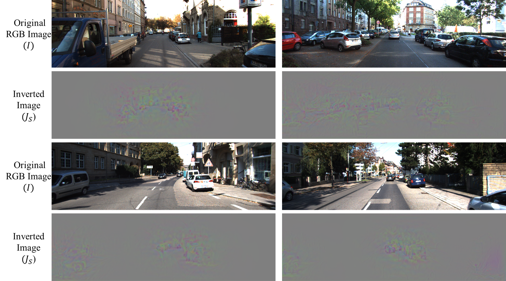
Figure 6: Model inversion examples of the DD3D source model in the “Lidar-input Target Model" experiments.

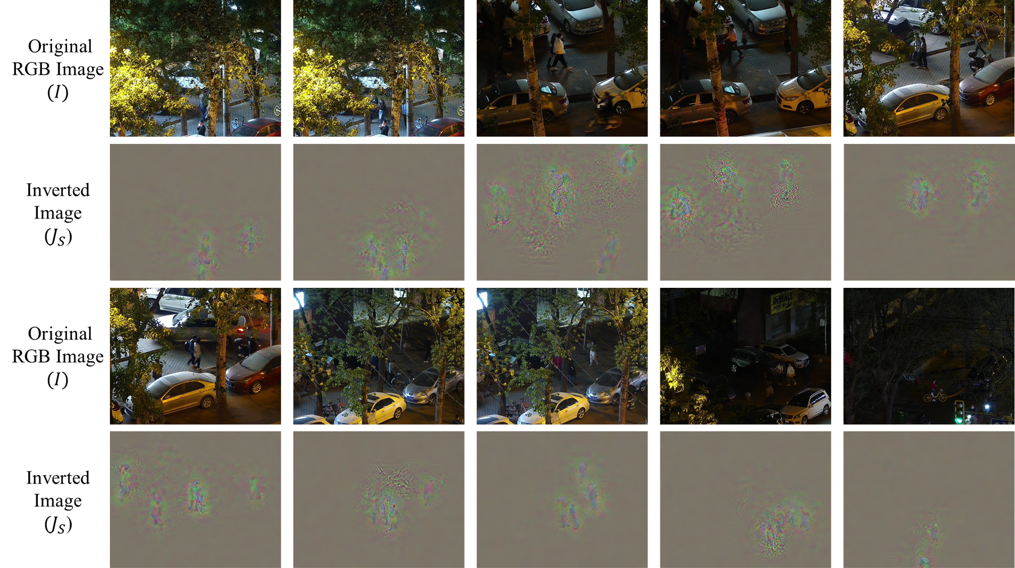
Figure 7: Model inversion examples of the R50-FPN-FasterRCNN source model in the “Infrared-input Target Model" experiments.

Target-modality Qualitative Results

In Figure 8, Figure 9, and Figure 10, we report more qualitative results on three target-modality input models. In all cases, the MAC-Self-supervised models that are trained on 0% target-modality annotations produce comparable or better than the best baseline models trained on 100% annotations. Trained on the same 100% target-modality annotations, the MAC-Supervised models clearly outperform the best baseline models.

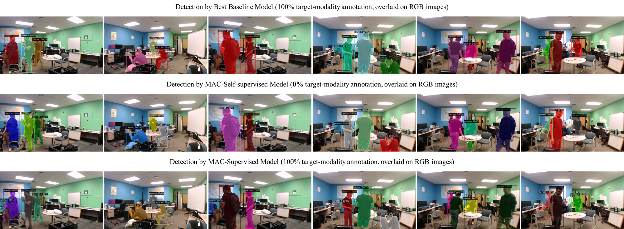
Figure 8: More Qualitative results on WiFi-input models (overlaid on RGB images).

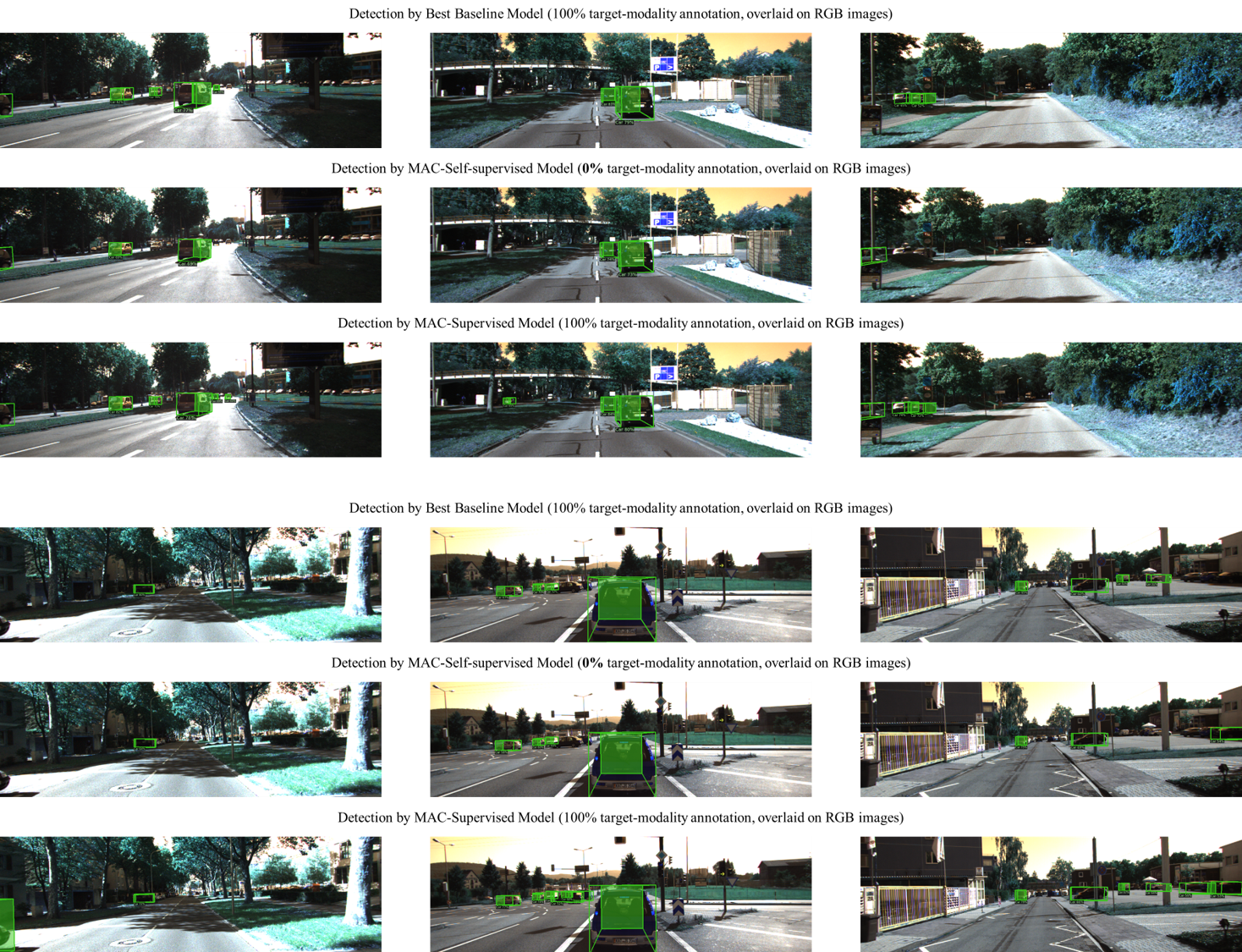
Figure 9: More Qualitative results on Lidar-input models (overlaid on RGB images).

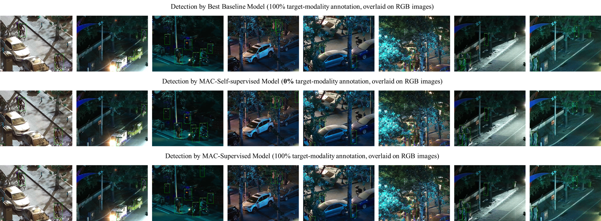
Figure 10: More Qualitative results on Infrared-input models (overlaid on RGB images).

References

- Zhao et al. [2018] Mingmin Zhao, Tianhong Li, Mohammad Abu Alsheikh, Yonglong Tian, Hang Zhao, Antonio Torralba, and Dina Katabi. Through-wall human pose estimation using radio signals. In CVPR, pages 7356–7365, 2018.
- Wang et al. [2019a] Fei Wang, Sanping Zhou, Stanislav Panev, Jinsong Han, and Dong Huang. Person-in-wifi: Fine-grained person perception using wifi. In ICCV, 2019a.
- Geiger et al. [2012] Andreas Geiger, Philip Lenz, and Raquel Urtasun. Are we ready for autonomous driving? the kitti vision benchmark suite. In CVPR, 2012.
- Sun et al. [2020] Pei Sun, Henrik Kretzschmar, Xerxes Dotiwalla, and et al. Scalability in perception for autonomous driving: Waymo open dataset. In CVPR, 2020.
- Hwang et al. [2015] Soonmin Hwang, Jaesik Park, Namil Kim, Yukyung Choi, and In So Kweon. Multispectral pedestrian detection: Benchmark dataset and baselines. In CVPR, 2015.
- Jia et al. [2021] Xinyu Jia, Chuang Zhu, Minzhen Li, Wenqi Tang, and Wenli Zhou. Llvip: A visible-infrared paired dataset for low-light vision. In Proceedings of the ICCV, pages 3496–3504, 2021.
- He et al. [2017] Kaiming He, Georgia Gkioxari, Piotr Dollár, and Ross B. Girshick. Mask R-CNN. CoRR, abs/1703.06870, 2017. URL http://arxiv.org/abs/1703.06870.
- Jocher et al. [2020] Glenn Jocher, Alex Stoken, Jirka Borovec, NanoCode012, ChristopherSTAN, Liu Changyu, Laughing, tkianai, Adam Hogan, lorenzomammana, yxNONG, AlexWang1900, Laurentiu Diaconu, Marc, wanghaoyang0106, ml5ah, Doug, Francisco Ingham, Frederik, Guilhen, Hatovix, Jake Poznanski, Jiacong Fang, Lijun Yu, changyu98, Mingyu Wang, Naman Gupta, Osama Akhtar, PetrDvoracek, and Prashant Rai. ultralytics/yolov5: v3.1 - Bug Fixes and Performance Improvements, October 2020. URL https://doi.org/10.5281/zenodo.4154370.
- Liu et al. [2021] Ze Liu, Yutong Lin, Yue Cao, Han Hu, Yixuan Wei, Zheng Zhang, Stephen Lin, and Baining Guo. Swin transformer: Hierarchical vision transformer using shifted windows. arXiv:2103.14030, 2021.
- Deng et al. [2009] J. Deng, W. Dong, R. Socher, L.-J. Li, K. Li, and L. Fei-Fei. ImageNet: A Large-Scale Hierarchical Image Database. In CVPR09, 2009.
- Lin et al. [2014] Tsung-Yi Lin, Michael Maire, Serge Belongie, James Hays, Pietro Perona, Deva Ramanan, Piotr Dollár, and C. Lawrence Zitnick. Microsoft coco: Common objects in context. In ECCV, Zürich, 2014. URL /se3/wp-content/uploads/2014/09/coco_eccv.pdf,http://mscoco.org.
- Kuznetsova et al. [2020] Alina Kuznetsova, Hassan Rom, Neil Alldrin, Jasper Uijlings, Ivan Krasin, Jordi Pont-Tuset, Shahab Kamali, Stefan Popov, Matteo Malloci, Alexander Kolesnikov, Tom Duerig, and Vittorio Ferrari. The open images dataset v4: Unified image classification, object detection, and visual relationship detection at scale. IJCV, 2020.
- He et al. [2018] Tong He, Zhi Zhang, Hang Zhang, Zhongyue Zhang, Junyuan Xie, and Mu Li. Bag of tricks for image classification with convolutional neural networks. arXiv:1812.01187, 2018.
- Zhang et al. [2019] Zhi Zhang, Tong He, Hang Zhang, Zhongyue Zhang, Junyuan Xie, and Mu Li. Bag of freebies for training object detection neural networks. arXiv:1902.04103, 2019.
- Ghiasi et al. [2020] Golnaz Ghiasi, Yin Cui, Aravind Srinivas, Rui Qian, Tsung-Yi Lin, Ekin D Cubuk, Quoc V Le, and Barret Zoph. Simple copy-paste is a strong data augmentation method for instance segmentation. arXiv:2012.07177, 2020.
- Wu et al. [2019] Yuxin Wu, Alexander Kirillov, Francisco Massa, Wan-Yen Lo, and Ross Girshick. Detectron2, 2019.
- Chen et al. [2019] Kai Chen, Jiaqi Wang, Jiangmiao Pang, Yuhang Cao, Yu Xiong, Xiaoxiao Li, Shuyang Sun, Wansen Feng, Ziwei Liu, Jiarui Xu, Zheng Zhang, Dazhi Cheng, Chenchen Zhu, Tianheng Cheng, Qijie Zhao, Buyu Li, Xin Lu, Rui Zhu, Yue Wu, Jifeng Dai, Jingdong Wang, Jianping Shi, Wanli Ouyang, Chen Change Loy, and Dahua Lin. MMDetection: Open mmlab detection toolbox and benchmark. arXiv:1906.07155, 2019.
- Qi et al. [2017] Charles R Qi, Li Yi, Hao Su, and Leonidas J Guibas. Pointnet++: Deep hierarchical feature learning on point sets in a metric space. arXiv:1706.02413, 2017.
- Kato et al. [2021] Sorachi Kato, Takeru Fukushima, T. Murakami, H. Abeysekera, Yusuke Iwasaki, T. Fujihashi, Takashi Watanabe, and S. Saruwatari. Csi2image: Image reconstruction from channel state information using generative adversarial networks. IEEE Access, 9:47154–47168, 2021.
- Kefayati et al. [2020] Mohammad Hadi Kefayati, Vahid Pourahmadi, and Hassan Aghaeinia. Wi2vi: Generating video frames from wifi csi samples. IEEE Sensors Journal, 20(19):11463–11473, 2020.
- Drob [2021] Michael Drob. Rf pix2pix unsupervised wi-fi to video translation. In arXiv:2102.09345, 2021.
- Milz et al. [2019] Stefan Milz, Martin Simon, Kai Fischer, and Maximillian Pöpperl. Points2pix: 3d point-cloud to image translation using conditional generative adversarial networks. arXiv:1901.09280, 2019.
- Limmer and Lensch [2019] Matthias Limmer and Hendrik P.A. Lensch. Infrared colorization using deep convolutional neural networks. arXiv:1604.02245, 2019.
- Rajendran et al. [2019] Rahul Rajendran, Thaweesak Trongtirakul, Thaweesak Trongtirakul, Karen Panetta, and Sos Agaian. A pixel-based color transfer system to recolor nighttime imagery. In Mobile Multimedia/Image Processing, Security, and Applications, 2019.
- Karras et al. [2020] Tero Karras, Samuli Laine, Miika Aittala, Janne Hellsten, Jaakko Lehtinen, and Timo Aila. Analyzing and improving the image quality of StyleGAN. In Proc. CVPR, 2020.
- Depatla and Mostofi [2018] S. Depatla and Y. Mostofi. Crowd counting through walls using wifi. In Proceedings of IEEE International Conference on Pervasive Computing and Communications, 2018.
- Liu et al. [2019a] Shangqing Liu, Yanchao Zhao, Fanggang Xue, Bing Chen, and Xiang Chen. Deepcount: Crowd counting with wifi via deep learning. arXiv:1903.05316, 2019a.
- Wang et al. [2017a] Wei Wang, Alex X. Liu, Muhammad Shahzad, Kang Ling, and Sanglu Lu. Device-free human activity recognition using commercial wifi devices. IEEE Journal on Selected Areas in Communications, 35(5):1118–1131, 2017a.
- Li et al. [2019] Heju Li, Xin He, Xukai Chen, Yinyin Fang, and Qun Fang. Wi-motion: A robust human activity recognition using wifi signals. IEEE Access, 7:153287 – 153299, 2019.
- Qi et al. [2016] Charles R Qi, Hao Su, Kaichun Mo, and Leonidas J Guibas. Pointnet: Deep learning on point sets for 3d classification and segmentation. arXiv:1612.00593, 2016.
- Shi et al. [2019] Shaoshuai Shi, Xiaogang Wang, and Hongsheng Li. Pointrcnn: 3d object proposal generation and detection from point cloud. In CVPR, June 2019.
- Yan et al. [2018] Yan Yan, Yuxing Mao, and Bo Li. Second: Sparsely embedded convolutional detection. Sensors, 2018.
- Lang et al. [2019] Alex H Lang, Sourabh Vora, Holger Caesar, Lubing Zhou, Jiong Yang, and Oscar Beijbom. Pointpillars: Fast encoders for object detection from point clouds. In CVPR, pages 12697–12705, 2019.
- Meyer et al. [2019] Gregory P Meyer, Ankit Laddha, Eric Kee, Carlos VallespiGonzalez, and Carl K Wellington. Lasernet: An efficient probabilistic 3d object detector for autonomous driving. In CVPR, page 12677–12686, 2019.
- Fan et al. [2021] Lue Fan, Xuan Xiong, Feng Wang, Naiyan Wang, and ZhaoXiang Zhang. Rangedet: In defense of range view for lidar-based 3d object detection. In ICCV, October 2021.
- Murez et al. [2018] Zak Murez, Soheil Kolouri, David Kriegman, Ravi Ramamoorthi, and Kyungnam Kim. Image to image translation for domain adaptation. In CVPR, 2018.
- Dou et al. [2018] Qi Dou, Cheng Ouyang, Cheng Chen, Hao Chen, and Pheng-Ann Heng. Unsupervised cross-modality domain adaptation of convnets for biomedical image segmentations with adversarial loss. In Proceedings of the 27th International Joint Conference on Artificial Intelligence (IJCAI), pages 691–697, 2018.
- Pizzati et al. [2020] Fabio Pizzati, Raoul de Charette, Michela Zaccaria, and Pietro Cerri. Domain bridge for unpaired image-to-image translation and unsupervised domain adaptation. In WACV, 2020.
- Musto and Zinelli [2020] Luigi Musto and Andrea Zinelli. Semantically adaptive image-to-image translation for domain adaptation of semantic segmentation. In BMVC, 2020.
- Xie et al. [2020] Xinpeng Xie, Jiawei Chen, Yuexiang Li, Linlin Shen, Kai Ma, and Yefeng Zheng. Self-supervised cyclegan for object-preserving image-to-image domain adaptation. In ECCV, 2020.
- Gal et al. [2021] Rinon Gal, Or Patashnik, Haggai Maron, Gal Chechik, and Daniel Cohen-Or. Stylegan-nada: Clip-guided domain adaptation of image generators, 2021.
- Hinton et al. [2015] Geoffrey Hinton, Oriol Vinyals, and Jeff Dean. Distilling the knowledge in a neural network. arXiv:1503.02531, 2015.
- Dhar et al. [2019] Prithviraj Dhar, Rajat Vikram Singh, Kuan-Chuan Peng, Ziyan Wu, and Rama Chellappa. Learning without memorizing. In CVPR, pages 5138–5146, 2019.
- Li and Hoiem [2017] Zhizhong Li and Derek Hoiem. Learning without forgetting. PAMI, 40(12):2935–2947, 2017.
- Romero et al. [2014] Adriana Romero, Nicolas Ballas, Samira Ebrahimi Kahou, Antoine Chassang, Carlo Gatta, and Yoshua Bengio. Fitnets: Hints for thin deep nets. arXiv:1412.6550, 2014.
- Wang et al. [2019b] Tao Wang, Li Yuan, Xiaopeng Zhang, and Jiashi Feng. Distilling object detectors with fine-grained feature imitation. In CVPR, pages 4933–4942, 2019b.
- Zagoruyko and Komodakis [2016] Sergey Zagoruyko and Nikos Komodakis. Paying more attention to attention: Improving the performance of convolutional neural networks via attention transfer. arXiv:1612.03928, 2016.
- Wang et al. [2017b] Fei Wang, Mengqing Jiang, Chen Qian, Shuo Yang, Cheng Li, Honggang Zhang, Xiaogang Wang, and Xiaoou Tang. Residual attention network for image classification. In CVPR, pages 3156–3164, 2017b.
- Liu et al. [2020] Xialei Liu, Hao Yang, Avinash Ravichandran, Rahul Bhotika, and Stefano Soatto. Continual universal object detection. arXiv:2002.05347, 2020.
- Chen et al. [2017] Guobin Chen, Wongun Choi, Xiang Yu, Tony Han, and Manmohan Chandraker. Learning efficient object detection models with knowledge distillation. In NIPS, pages 742–751, 2017.
- Gupta et al. [2016] Saurabh Gupta, Judy Hoffman, and Jitendra Malik. Cross modal distillation for supervision transfer. In CVPR, 2016.
- Zoph et al. [2020] Barret Zoph, Ekin D. Cubuk, Golnaz Ghiasi, Tsung-Yi Lin, Jonathon Shlens, and Quoc V. Le. Learning data augmentation strategies for object detection. In ECCV, 2020.
- Kim et al. [2021] JangHyun Kim, Wonho Choo, Hosan Jeong, and Hyun Oh Song. Co-mixup: Saliency guided joint mixup with supermodular diversity. In International Conference on Learning Representations, 2021.
- Zhong et al. [2017] Zhun Zhong, Liang Zheng, Guoliang Kang, Shaozi Li, and Yi Yang. Random erasing data augmentation. arXiv:1708.04896, 2017.
- Huang et al. [2020a] Zeyi Huang, Wei Ke, and Dong Huang. Improving object detection with inverted attention. In WACV, 2020a.
- Huang et al. [2020b] Zeyi Huang, Haohan Wang, Eric P. Xing, and Dong Huang. Self-challenging improves cross-domain generalization. In ECCV, 2020b.
- Chen et al. [2020] Shuhan Chen, Xiuli Tan, Ben Wang, Huchuan Lu, Xuelong Hu, and Yun Fu. Reverse attention based residual network for salient object detection. TIP, 29:3763–3776, 2020.
- Hou et al. [2019] Yuenan Hou, Zheng Ma, Chunxiao Liu, and Chen Change Loy. Learning lightweight lane detection cnns by self attention distillation. In ICCV, pages 1013–1021, 2019.
- Wang et al. [2019c] Lezi Wang, Ziyan Wu, Srikrishna Karanam, Kuan-Chuan Peng, Rajat Vikram Singh, Bo Liu, and Dimitris N Metaxas. Sharpen focus: Learning with attention separability and consistency. In ICCV, pages 512–521, 2019c.
- Huang et al. [2020c] Zeyi Huang, Yang Zou, BVK Kumar, and Dong Huang. Comprehensive attention self-distillation for weakly-supervised object detection. NIPS, 33, 2020c.
- Rabbi et al. [2020] Jakaria Rabbi, Nilanjan Ray, Matthias Schubert, Subir Chowdhury, and Dennis Chao. Small-object detection in remote sensing images with end-to-end edge-enhanced gan and object detector network. Remote Sensing, 12(9):1432, 2020.
- Liu et al. [2019b] Lanlan Liu, Michael Muelly, Jia Deng, Tomas Pfister, and Jia Li. Generative modeling for small-data object detection. In ICCV, 2019b.
- van den Oord et al. [2017] Aaron van den Oord, Oriol Vinyals, and Koray Kavukcuoglu. Neural discrete representation learning. arXiv:1711.00937, 2017.
- Razavi et al. [2019] Ali Razavi, Aaron van den Oord, and Oriol Vinyals. Generating diverse high-fidelity images with vq-vae-2. arXiv:1906.00446, 2019.
- Esser et al. [2021] Patrick Esser, Robin Rombach, and Bjorn Ommer. Taming transformers for high-resolution image synthesis. arXiv:2012.09841, 2021.
- Zhou et al. [2016] Bolei Zhou, Aditya Khosla, Agata Lapedriza, Aude Oliva, and Antonio Torralba. Learning deep features for discriminative localization. In CVPR, pages 2921–2929, 2016.
- Halperin et al. [2011] Daniel Halperin, Wenjun Hu, Anmol Sheth, and David Wetherall. Tool release: Gathering 802.11 n traces with channel state information. ACM SIGCOMM Computer Communication Review, 41(1):53–53, 2011.
- Bengio et al. [1994] Y. Bengio, P. Simard, and P. Frasconi. Learning long-term dependencies with gradient descent is difficult. IEEE Transactions on Neural Networks, 5(2):157––166, 1994.
- Glorot and Bengio [2010] X. Glorot and Y. Bengio. Understanding the difficulty of training deep feedforward neural networks. In AISTATS, 2010.
- Vondrick et al. [2013] C. Vondrick, A. Khosla, T. Malisiewicz, and A. Torralba. HOGgles: Visualizing Object Detection Features. ICCV, 2013.
- Cao and Johnson [2021] Ang Cao and Justin Johnson. Inverting and understanding object detectors. arXiv:2106.13933, 2021.
- Park et al. [2021] Dennis Park, Rares Ambrus, Vitor Guizilini, Jie Li, and Adrien Gaidon. Is pseudo-lidar needed for monocular 3d object detection? In ICCV, 2021.
- Simonelli et al. [2020] Andrea Simonelli, Samuel Rota Bulo, Lorenzo Porzi, Manuel Lopez Antequera, and Peter Kontschieder. Disentangling monocular 3d object detection: From single to multiclass recognition. PAMI, 2020.
- Zhang and Ma [2021] Linfeng Zhang and Kaisheng Ma. Improve object detection with feature-based knowledge distillation: Towards accurate and efficient detectors. In ICLR, 2021.