Signal reconstruction using determinantal sampling

Abstract

We study the approximation of a square-integrable function from a finite number of evaluations on a random set of nodes according to a well-chosen distribution. This is particularly relevant when the function is assumed to belong to a reproducing kernel Hilbert space (RKHS). This work proposes to combine several natural finite-dimensional approximations based two possible probability distributions of nodes. These distributions are related to determinantal point processes, and use the kernel of the RKHS to favor RKHS-adapted regularity in the random design. While previous work on determinantal sampling relied on the RKHS norm, we prove mean-square guarantees in $L^{2}$ norm. We show that determinantal point processes and mixtures thereof can yield fast convergence rates. Our results also shed light on how the rate changes as more smoothness is assumed, a phenomenon known as superconvergence. Besides, determinantal sampling generalizes i.i.d. sampling from the Christoffel function which is standard in the literature. More importantly, determinantal sampling guarantees the so-called instance optimality property for a smaller number of function evaluations than i.i.d. sampling.

Keywords— Christoffel sampling; instance optimality property; finite-dimensional approximations; determinantal point processes; reproducing kernel Hilbert spaces.

1 Introduction

The problem of reconstructing a continuous signal from a set of discrete samples is a fundamental question of sampling theory. It has stimulated a considerable literature. This problem consists in approximating an unknown function $f$ by a surrogate $\hat{f}$ knowing a discrete set of evaluations of $f$. The Whittaker-Shannon-Kotel’nikov (WSK) sampling theorem is arguably the most emblematic result in the field. It can be seen as an exact interpolation result from periodic samples for functions that are band-limited in the Fourier domain (Whittaker, 1928; Shannon, 1949; Kotel’nikov, 2006). This theorem has been extended to functions that are band-limited with respect to other transforms than Fourier including, for instance, Sturm-Liouville transforms (Kramer, 1959; Campbell, 1964), Laguerre transforms (Jerri, 1976) and Jacobi transforms (Koornwinder and Walter, 1990).

Reproducing kernel Hilbert spaces (RKHSs) and sampling problems have a long common history. Tracing back to (Aronszajn, 1943, 1950), one possible interpretation of the definition of an RKHS $\mathcal{F}$ of kernel $k$ is that any signal $f\in\mathcal{F}$ is a limit of weighted sums of kernel translates $k(x,\cdot)$. In a seminal paper, Yao (1967) derived sufficient conditions on a configuration of nodes $(x_{i})_{i\in\mathcal{I}}$ to achieve exact reconstruction of any element $f$ of the RKHS $\mathcal{F}$, i.e., to ensure that uniformly,

$$f=\sum\limits_{i\in\mathcal{I}}f(x_{i})k(x_{i},\cdot).$$ (1)

This is essential to signal processing that Yao proved that the spaces of band-limited signals in the Fourier, Bessel, or cosine domains are all RKHSs. In particular, Yao’s result generalizes the WSK theorem. Weaker sufficient conditions than Yao’s for (1) to hold have been studied, see e.g. (Nashed and Walter, 1991). However the WSK sampling theorem and its extensions to RKHSs remain asymptotic: an infinite number of samples is required in order to guarantee the exact reconstruction of the function. In real applications, only a finite number of evaluations $f(x_{1}),\dots,f(x_{N})$, at nodes $x_{1},\dots,x_{N}\in\mathcal{X}$, is available. Therefore non-asymptotic guarantees on reconstructions from $N$ samples are necessary. They are the purpose of the present work.

Interestingly, the problem of reconstruction from a finite number of evaluations arose first historically, as mentioned by Higgins (1985). Indeed, an early form of sampling theorem may be traced back to an interpolation scheme due to de La Vallée Poussin (1908); see (Butzer and Stens, 1992) for a historical account. Non-asymptotic sampling results have resurged in popularity recently (Cohen and Migliorati, 2017; Bach, 2017a; Avron et al., 2019). In those works, the nodes $x_{1},\dots,x_{N}$ were taken to be independent draws from a particular probability distribution. The latter is closely related to extensions of the so-called Christoffel function, a classical tool in the theory of orthogonal polynomials (Nevai, 1986). These configurations of independent particles were shown to yield approximations that satisfy the instance optimality property (IOP). IOP provides a desirable multiplicative error bound that guarantees exact recovery on a finite-dimensional subspace, with an almost optimal number of nodes. On the other hand, alternative designs have been proposed to achieve optimal reconstruction, using boosting (Haberstich et al., 2022) or sparsification techniques (Krieg and Ullrich, 2021; Dolbeault and Cohen, 2022a; Dolbeault et al., 2023; Chkifa and Dolbeault, 2023).

This work presents a general approach for signal reconstruction, based on non-independent random nodes. The key idea is to use random nodes sampled from mixtures of determinantal point processes (DPP). DPPs are distributions over configurations of points that encode repulsion in the form of a kernel: connecting the DPP’s kernel to the RKHS kernel makes the nodes to repel with an repulsion related to the smoothness of the target function. DPPs were introduced in Odile Macchi’s 1972 thesis –recently translated and reprinted as (Macchi, 2017)– as models for detection times in fermionic optics. Since then, they have been thoroughly studied in random matrix theory (Johansson, 2005), and have more recently been adopted in machine learning (Kulesza and Taskar, 2012), spatial statistics (Lavancier et al., 2015), and Monte Carlo methods (Bardenet and Hardy, 2020).

The proposed non-asymptotic guarantees for function reconstruction with DPPs are motivated by previous works on numerical integration (Belhadji et al., 2019, 2020). In these works, we measured reconstruction performance using the RKHS norm. Then a rather strong smoothness assumption appeared necessary to ensure that the function belong to a particular strict subspace of the RKHS. Now motivated by applications in signal reconstruction, and to overcome the smoothness assumption of previous works, an alternative analysis is proposed that replaces the RKHS norm by the $L_{2}$ norm. In particular, we study various finite-dimensional approximations of a function living in an RKHS, such as the least-squares approximation with respect to the $L_{2}$ norm. We show that its mean square error converges to zero at a rate that depends on the eigenvalues of the RKHS kernel. Moreover, we show that the convergence is faster for functions living in a certain low-dimensional subspace of the RKHS. This sheds light on the phenomenon of superconvergence observed in the literature of kernel-based approximations (Schaback, 2018), and relates to the question of completeness of DPPs (Lyons, 2014). Yet, in spite of its remarkable theoretical properties, the least-squares approximation with respect to the $L_{2}$ norm cannot be evaluated numerically by using a finite number of evaluations of the target function only. For this reason, we also investigate more practical approximations based on two particular transforms, i.e. linear operators from the RKHS to finite-dimensional vector spaces, built through a compilation of quadrature rules. In particular, we prove that the aforementioned instance optimality property holds for a particular transform-based approximation using DPPs, even with a minimal sampling budget. Numerical experiments in dimension one as well as on the hypersphere validate our results experimentally. They show the very good empirical efficiency of the proposed approximations. Even though our bounds guarantee good performance, the numerical performance actually exceeds the expectations, which shows as well that there is still some room for improvement of our theoretical results.

This article is organized as follows. Section 2 contains notations and definitions, as well as a brief review of previous work on the reconstruction of RKHS functions based on discrete samples. In Section 3, we present our main results. In Section 4, we illustrate our results and compare to related work using numerical simulations. In Sections 5 and 6, we discuss a number of open questions and conclude.

2 Sampling and reconstruction in RKHSs

In Section 2.1.1, for ease of reference, we introduce some basic notation and assumptions to be used throughout the paper. In Section 2.1.2, we define fractional subspaces, which correspond to increasing levels of smoothness within an RKHS. In Section 2.2, we recall the finite-dimensional approximations that we will work with in the rest of the article. To give historical context, Section 2.3 and Section 2.4 are devoted to related works on the topic. The contents of these two sections may be skipped in a first read except for Section 2.3.2 which is necessary for the statement of the main results presented in Section 3.

2.1 Kernels and RKHSs

2.1.1 Notations and assumptions

Let $\mathcal{X}$ be a metric set, equipped with a positive Borel measure $\omega$. Let $k:\mathcal{X}\times\mathcal{X}\rightarrow\mathbb{R}$ be a symmetric, positive definite kernel. Consider the inner product defined on the space $\mathcal{F}_{0}$ of finite linear combinations of kernel translates by

$$\left\langle\sum_{i=1}^{m}a_{i}k(x_{i},\cdot),\sum_{j=1}^{n}b_{j}k(y_{j},\cdot)\right\rangle_{\mathcal{F}}=\sum_{i=1}^{m}\sum_{j=1}^{n}a_{i}b_{j}k(x_{i},y_{j}),$$ (2)

where $a_{1},b_{1},\dots\in\mathbb{R}$ and $x_{1},y_{1},\dots\in\mathcal{X}$. In the sequel, $[N]$ will denote the set of indices ranging from $1$ to $N$. The completion $\mathcal{F}$ of $\mathcal{F}_{0}$ for $\langle\cdot,\cdot\rangle_{\mathcal{F}}$ is the so-called reproducing kernel Hilbert space of kernel $k$. By the Moore-Aronszajn theorem, it is the unique Hilbert space of functions that satisfies the reproducing property, i.e., for all $f\in\mathcal{F}$ and $x\in\mathcal{X}$, $f(x)=\langle f,k(x,\cdot)\rangle_{\mathcal{F}}$; see e.g. (Berlinet and Thomas-Agnan, 2011) for a general reference.

The properties of a function in $\mathcal{F}$ are often described in terms of the spectral characteristics of the integral operator of kernel $k$, at the price of some additional technicalities. Because we shall need a so-called Mercer decomposition, we follow here the precise reference paper of Steinwart and Scovel (2012). A convenient way to diagonalize the operator $\bm{\Sigma}$ defined by

$$\bm{\Sigma}f(x)=\int k(x,y)f(y)\mathrm{d}\omega(y)$$ (3)

is to make sure it defines a compact operator from $\operatorname{\mathbb{L}_{2}(\omega)}$ to itself. A practical sufficient condition for this compactness to hold is that $\int_{\mathcal{X}}k(x,x)\mathrm{d}\omega(x)<+\infty$; see (Steinwart and Scovel, 2012, Lemma 2.3). This is in particular implied by our Assumptions 1 and 2, whose additional strength we shall later require.

Assumption 1.

The diagonal of the kernel $x\mapsto k(x,x)$ is bounded in $\mathcal{X}$.

We note that the positive definiteness of $k$ implies that for all $x,y$,

$$k(x,x)k(y,y)-k(x,y)^{2}\geq 0,$$

so that under Assumption 1, $x,y\mapsto k(x,y)$ is bounded in $\mathcal{X}\times\mathcal{X}$.

Assumption 2.

The measure $\omega$ is finite, i.e. $\int_{\mathcal{X}}\mathrm{d}\omega(x)<+\infty$.

Under Assumptions 1 and 2, $\bm{\Sigma}$ in (3) is a self-adjoint, non-negative, compact operator. The spectral theorem, see e.g. Chapter 6 in (Brezis, 2010), guarantees the existence of an orthonormal basis $(\widetilde{e}_{m})_{m\in\mathbb{N}^{*}}$ of $\operatorname{\mathbb{L}_{2}(\omega)}$ and a family of non-increasing non-negative scalars $(\sigma_{m})_{m\in\mathbb{N}^{*}}$ such that $\bm{\Sigma}\widetilde{e}_{m}=\sigma_{m}\widetilde{e}_{m}$ for $m\in\mathbb{N}^{*}$. We now make extra assumptions to reach a Mercer decomposition.

Assumption 3.

The kernel $k$ is continuous, $\omega$ has full support, and $\sigma_{m}>0$ for all $m\in\mathbb{N}^{*}$.

Under Assumptions 1 to 3, it is easy to see that $\bm{\Sigma}$ maps to continuous functions, so that $\widetilde{e}_{m}=\frac{1}{\sigma_{m}}\bm{\Sigma}\widetilde{e}_{m}$ has a continuous representative $e_{m}$ in its equivalence class in $\operatorname{\mathbb{L}_{2}(\omega)}$. Letting $e_{m}^{\mathcal{F}}:=\sqrt{\sigma_{m}}e_{m}$, the family $(e_{m}^{\mathcal{F}})_{m\in\mathbb{N}^{*}}$ is then an orthonormal basis of $\mathcal{F}$, and $\mathcal{F}$ is isometrically isomorphic to a dense subspace of $\operatorname{\mathbb{L}_{2}(\omega)}$ through

$$\sum a_{i}e_{i}^{\mathcal{F}}\mapsto\sum\sigma_{m}^{1/2}a_{i}\widetilde{e}_{i};$$ (4)

see (Steinwart and Scovel, 2012, Theorem 2.11, Lemma 2.12, and Corollary 3.5). In particular, it is customary to (abusively) write $\mathcal{F}=\bm{\Sigma}^{1/2}\operatorname{\mathbb{L}_{2}(\omega)}$ and, for $f\in\mathcal{F}$,

$$\|f\|_{\operatorname{\mathcal{F}}}^{2}=\|\bm{\Sigma}^{-1/2}f\|_{\omega}^{2}=\sum\limits_{m\in\mathbb{N}^{*}}\frac{\langle f,e_{m}\rangle_{\omega}^{2}}{\sigma_{m}}<+\infty.$$ (5)

Finally, by (Steinwart and Scovel, 2012, Corollary 3.5), for any $x\in\mathcal{X}$, we can write the so-called Mercer decomposition,

$$k(x,y)=\langle k(x,\cdot),k(y,\cdot)\rangle_{\mathcal{F}}=\sum\limits_{m\in\mathbb{N}^{*}}e_{m}^{\operatorname{\mathcal{F}}}(x)e_{m}^{\operatorname{\mathcal{F}}}(y)=\sum\limits_{m\in\mathbb{N}^{*}}\sigma_{m}e_{m}(x)e_{m}(y).$$ (6)

where the convergence is uniform in $y\in\mathcal{X}$. Assumptions 1, 2, and 3 hold for the rest of this article.

2.1.2 Increasing levels of smoothness

Figure 1: A schematic diagram illustrating the relationship between the unit ball $\mathbb{B}_{\mathbb{L}_{2}(\omega)}$ of $\mathbb{L}_{2}(\omega)$, the unit ball $\mathbb{B}_{\operatorname{\mathcal{F}}}$ of $\operatorname{\mathcal{F}}$, and the image of $\mathbb{B}_{\mathbb{L}_{2}(\omega)}$ by the integration operator $\bm{\Sigma}$.

The fact that $\mathcal{F}=\bm{\Sigma}^{1/2}\mathbb{L}_{2}(\omega)$ illustrates the smoothing nature of the integral operator $\bm{\Sigma}$. Similarly, for $r\geq 0$, an element $g\in\mathbb{L}_{2}(\omega)$ belongs to $\bm{\Sigma}^{r+1/2}\mathbb{L}_{2}(\omega)$ if and only if

$$\sum_{m\in\mathbb{N}^{*}}\frac{\langle g,e_{m}\rangle_{\omega}^{2}}{\sigma_{m}^{2r+1}}<+\infty.$$ (7)

Moreover, since $(\sigma_{m})$ is a (non-increasing) sequence of positive real numbers, we have

$$r\geq r^{\prime}\geq 0\implies\bm{\Sigma}^{r+1/2}\mathbb{L}_{2}(\omega)\subset\bm{\Sigma}^{r^{\prime}+1/2}\mathbb{L}_{2}(\omega).$$ (8)

In particular, for $r\geq 0$, $\bm{\Sigma}^{r+1/2}\mathbb{L}_{2}(\omega)\subset\operatorname{\mathcal{F}}$: these subspaces define increasing levels of regularity in the RKHS $\operatorname{\mathcal{F}}$. Figure 1 illustrates this hierarchy of functional spaces.

2.2 Finite-dimensional approximations in RKHSs

The reconstruction of a function $f$ that belongs to an RKHS $\mathcal{F}$ based on its evaluations over a finite set of nodes $x_{1},\dots x_{N}\in\mathcal{X}$ can be achieved by different families of finite-dimensional approximations. The following approximations will be of interest for the rest of the article.

2.2.1 Approximations based on mixtures of kernel translates

By definition of an RKHS, a natural choice of approximation is a weighted sum of kernel functions. Formally, the objective is thus to build a set of nodes $(x_{i})$, a.k.a. a design, and weights $(w_{i})$, such that a suitable norm of the residual

$$f-\sum_{i\in[N]}w_{i}k(x_{i},\cdot)$$ (9)

is small. Assuming the design $\bm{x}=(x_{i})_{i\in[N]}$ is fixed, we now consider two possible choices for this norm that induce different sets of weights.

Minimizing the $\operatorname{\mathbb{L}_{2}(\omega)}$ norm of the residual (9) yields the classical least-squares (LS) approximation

$$\hat{f}_{\mathrm{LS},\bm{x}}=\arg\min_{\bm{w}\in\mathbb{R}^{N}}\|f-\sum\limits_{i\in[N]}w_{i}k(x_{i},\cdot)\|_{\omega}^{2}.$$ (10)

The least-squares approximation typically enjoys strong theoretical properties. However, we shall see in Section 3.1 that computing the optimal weights in (10) requires the evaluation of $\bm{\Sigma}f$ at the nodes $x_{1},\dots,x_{N}$. This makes the method impractical, and calls for more tractable approximations.

The RKHS norm of the residual is a natural alternative objective to minimize, and yields the so-called optimal kernel approximation (OKA)

$$\hat{f}_{\mathrm{OKA},\bm{x}}=\arg\min\limits_{\bm{w}\in\mathbb{R}^{N}}\|f-\sum\limits_{i\in[N]}w_{i}k(x_{i},\cdot)\|_{\operatorname{\mathcal{F}}}.$$ (11)

We shall sometimes write $\hat{f}_{\mathrm{OKA}}$ for $\hat{f}_{\mathrm{OKA},\bm{x}}$ when the design $\bm{x}$ is clear from the context. Let us observe that the approximation (11) is uniquely defined if the matrix $\bm{K}(\bm{x})=(k(x_{i},x_{i^{\prime}}))_{i,i^{\prime}\in[N]}$ is non-singular. The optimal vector of weights is then simply $\widehat{\bm{w}}_{\mathrm{OKA},\bm{x}}:=\bm{K}(\bm{x})^{-1}f(\bm{x})$; unlike the least-squared approximation, computing the weights depends on being able to evaluate $f$ at the nodes only. Moreover, OKA comes with a remarkable interpolation property: for $i\in[N]$, $\hat{f}_{\mathrm{OKA},\bm{x}}(x_{i})=f(x_{i})$.

2.2.2 Approximations living in eigenspaces

Another way to recover a continuous signal $f\in\operatorname{\mathcal{F}}$ from its evaluations $f(x_{1}),\dots,f(x_{N})$ at fixed nodes, is to seek an approximation that belongs to the eigenspace $\mathcal{E}_{M}=\mathrm{Span}(e_{1},\dots,e_{M})$ for some $M\in\mathbb{N}^{*}$. We consider two such approaches.

Transform-based approximations.

Consider the projection of $f$ onto $\mathcal{E}_{M}$,

$$f_{M}:=\sum_{m\in[M]}\langle f,e_{m}\rangle_{\omega}e_{m}.$$ (12)

Note that, for $m\in[M]$, $\langle f,e_{m}\rangle_{\omega}$ is the integral $I_{m}(f):=\int_{\mathcal{X}}f(x)e_{m}(x)\mathrm{d}\omega(x)$. Since we want to assume only the availability of the evaluation of $f$ at the nodes, we consider approximating each integral $I_{m}(f)$ by a weighted sum

$$\hat{I}_{m}(f):=\sum_{i\in[N]}\alpha_{m,i}f(x_{i}),$$ (13)

where $\alpha_{m,i}$ are quadrature weights to be discussed shortly. The collection of operators $\hat{I}_{m}$ form a transform $\Phi$, defined as $\Phi(f)=(\hat{I}_{m}(f))_{m\in[M]}\in\mathbb{R}^{M}$. The resulting approximation $\hat{f}_{\Phi}$ will be called a transform-based approximation of $f$. Note that

$$\hat{f}_{\Phi}:=\sum_{m\in[M]}\hat{I}_{m}(f)e_{m}=\sum_{i\in[N]}\left(\sum_{m\in[M]}\alpha_{m,i}\right)f(x_{i}),$$ (14)

is a weighted sum of evaluations of $f$ at the nodes $(x_{i})$.

For the construction of the quadrature weights $(\alpha_{m,i})$ in (13), this work focuses on interpolative quadrature rules (Larkin, 1972): given a kernel $\kappa:\mathcal{X}\times\mathcal{X}\rightarrow\mathbb{R}$, the weights $\alpha_{m,i}$ of an interpolative quadrature are chosen so that

$$\forall i\in[N],m\in[N],\>\>\hat{I}_{m}(\kappa(x_{i},\cdot))=I_{m}(\kappa(x_{i},\cdot)).$$ (15)

Under the assumption that the functions $\kappa(x_{1},\cdot),\dots,\kappa(x_{N},\cdot)$ are linearly independent, the sequence $(\alpha_{m,i})_{(m,i)\in[N]\times[N]}$ is uniquely defined by (15). We now single out two such interpolative quadratures, corresponding to two choices for $\kappa$.

In general, (15) only holds for $\hat{I}_{1},\dots,\hat{I}_{N}$. Yet, when $\kappa=k$, the property (15) extends to $\hat{I}_{m}$ for $m>N$ as well. Indeed, when $\kappa=k$, we have $I_{m}(\kappa(x,\cdot))=\sigma_{m}e_{m}(x)$ for $x\in\mathcal{X}$, so that (15) implies that the vector $\bm{\alpha}_{m}=\bm{\alpha}_{m}^{\mathrm{OKQ}}:=(\alpha_{m,i}^{\mathrm{OKQ}})_{i\in[N]}$ satisfies

$$\bm{\alpha}_{m}^{\mathrm{OKQ}}=\sigma_{m}\bm{K}(\bm{x})^{-1}e_{m}(\bm{x}),$$ (16)

under the assumption that the matrix $\bm{K}(\bm{x})$ is non-singular. In other words, the vector $\bm{\alpha}_{m}^{\mathrm{OKQ}}$ is nothing but the minimizer of (11) when $f$ is $\sigma_{m}e_{m}$. We name the resulting quadrature rule the optimal kernel quadrature (OKQ). In the rest of the article, the corresponding transform will be called the optimal kernel quadrature transform; the corresponding quadrature rules are denoted by $\hat{I}_{1}^{\mathrm{OKQ}},\dots,\hat{I}_{M}^{\mathrm{OKQ}}$, and the resulting approximation (14) by $\hat{f}_{\mathrm{OKQ},M,\bm{x}}$.

Alternately, taking $\kappa$ equal to $k_{N}(x,y):=\sum_{n\in[N]}e_{n}(x)e_{n}(y)$ in (15), we require that

$$\forall m,m^{\prime}\in[N],\>\>\hat{I}_{m}(e_{m^{\prime}})=\delta_{m,m^{\prime}},$$ (17)

which is reminiscent of a property satisfied by Gaussian quadrature (Gautschi, 2004). This yields new quadrature weights in (13),

$$\bm{\alpha}_{m}^{\mathrm{QI}}=\bm{K}_{N}(\bm{x})^{-1}e_{m}(\bm{x}),\quad m\in[N],$$ (18)

where $\bm{K}_{N}(\bm{x}):=(k_{N}(x_{i},x_{i^{\prime}}))_{i,i^{\prime}\in[N]}$. Note the similarity with (16). Except for some exceptional families of functions such as orthogonal polynomials, the quadrature weights (18) do not guarantee that (15) can be extended to $m>N$. Finally, note that the resulting approximation, denoted by $\hat{f}_{\mathrm{QI},N,\bm{x}}$ has been called quasi-interpolant (QI) or hyperinterpolant in the literature (Sloan, 1995), since

$$\forall f\in\mathcal{E}_{M}=\mathrm{Span}(e_{1},\dots,e_{M}),\quad\hat{f}_{\mathrm{QI},M,\bm{x}}=f=f_{M}.$$ (19)

In the rest of the article, we denote the corresponding quadrature rules by $\hat{I}^{\mathrm{QI}}_{1},\dots,\hat{I}^{\mathrm{QI}}_{N}$. Note that, for $m\in[N]$, $\hat{I}^{\mathrm{QI}}_{m}$ depends on $N$ and $\bm{x}$ that are dropped from the notation for simplicity.

The empirical least-squares approximation.

Let $\bm{x}\in\mathcal{X}^{N}$ and $q:\mathcal{X}\rightarrow\mathbb{R}_{+}^{*}$. Consider the so-called empirical semi-norm $\|.\|_{q,\bm{x}}$ defined on $\mathbb{L}_{2}(\omega)$ by

$$\|h\|_{q,\bm{x}}^{2}:=\frac{1}{N}\sum\limits_{i=1}^{N}q(x_{i})h(x_{i})^{2}.$$ (20)

The empirical least-squares estimator yields yet another approximation

$$\hat{f}_{\mathrm{ELS},M,\bm{x}}:=\operatorname*{arg\,min}_{\hat{f}\in\mathcal{E}_{M}}\|f-\hat{f}\|_{q,\bm{x}}^{2},$$ (21)

We discuss the choice of $q$ and the design $\bm{x}$ in Section 2.3.1. The intuition is that, for well-chosen weight $q$ and design $\bm{x}$, the semi-norm $\|.\|_{q,\bm{x}}$ is supposed to “mimic” the $\|.\|_{\omega}$ norm as $N$ goes to infinity. Similarly, $\hat{f}_{\mathrm{ELS},M,\bm{x}}$ is supposed to inherit some of the properties of $f_{M}$, the projection of $f$ onto $\mathcal{E}_{M}$. Compared to $\hat{f}_{\mathrm{LS},\bm{x}}$, the approximation $\hat{f}_{\mathrm{ELS},M,\bm{x}}$ has the advantage of being computable given the evaluations of $f$ at the nodes $\bm{x}$. Indeed, Cohen et al. (2013) show that writing $\hat{f}_{\mathrm{ELS},M,\bm{x}}=\sum_{m=1}^{M}w_{m}e_{m}$ yields

$$\bm{G}_{q,\bm{x}}\bm{w}=\bm{d}_{q,\bm{x}},$$ (22)

where $\bm{G}_{q,\bm{x}}=(\langle e_{m},e_{m^{\prime}}\rangle_{q,\bm{x}})_{m,m^{\prime}\in[M]}\in\mathbb{R}^{M\times M}$ is the Gramian matrix of the family $(e_{m})_{m\in[M]}$ with respect to the inner product defined by (20), and $\bm{d}_{q,\bm{x}}=(d_{m})_{m\in[M]}\in\mathbb{R}^{M}$ is defined by

$$d_{m}:=\sum_{i=1}^{N}q(x_{i})f(x_{i})e_{m}(x_{i})/N,\quad m\in[M].$$

In other words, the numerical evaluation of $\hat{f}_{\mathrm{ELS},M,\bm{x}}$ requires to solve the linear system (22). This in turn requires the evaluation of $\bm{G}_{q,\bm{x}}$ and $\bm{d}_{q,\bm{x}}$, which boils down to the evaluation of the functions $f$, $e_{m}$ and $q$ on the nodes $x_{1},\dots,x_{N}$. Moreover, $\hat{f}_{\mathrm{ELS},M,\bm{x}}$ is uniquely defined if and only if $\bm{G}_{q,\bm{x}}$ is non-singular.

2.3 Designs for finite-dimensional approximations

An abundant literature provides theoretical guarantees for the finite-dimensional approximations presented in Section 2.2; this includes, but is not limited to, (Erdős and Turán, 1937; Sloan, 1995; Wendland, 2004; Schaback and Wendland, 2006). These results deal with specific RKHSs, and cannot be easily generalized to an arbitrary RKHS. Recently, a new tendency has emerged that looks for a universal sampling approach that is valid for a large class of RKHSs. This section first provides an overview of this universal sampling literature. In the same spirit, we then show that determinantal point processes (DPPs) offer an adequate framework to design configurations of nodes with strong theoretical guarantees for finite-dimensional approximations, in a wide family of RKHSs.

2.3.1 Independent samples from the Christoffel function

The last decade has seen significant progress in the study of function reconstruction based on randomized configurations (Cohen et al., 2013; Hampton and Doostan, 2015; Cohen and Migliorati, 2017; Adcock and Cardenas, 2020; Adcock et al., 2022; Dolbeault and Cohen, 2022a). These works focused on the study of the empirical least-squares approximation; see Section 2.2.2. In particular, the so-called instance optimality property (IOP) has been a matter of extensive investigation. The idea is to find assumptions on the configuration $\bm{x}$, the function $q:\mathcal{X}\rightarrow\mathbb{R}_{+}^{*}$, and the order $M\leq N$, under which we can certify that

$$\forall f\in\mathcal{F},\>\>\|f-\hat{f}_{\mathrm{ELS},M,\bm{x}}\|_{\omega}\leq C\|f-f_{M}\|_{\omega},$$ (23)

where $C>0$ is a constant. Instance optimality implies that $\hat{f}_{\mathrm{ELS},M,\bm{x}}=f$ for $f\in\mathcal{E}_{M}$, so that the reconstruction is exact in the eigenspace $\mathcal{E}_{M}$. Moreover, it provides an upper bound of the approximation error $\|f-\hat{f}_{\mathrm{ELS},M,\bm{x}}\|_{\omega}$ for generic functions. Investigating necessary conditions for the IOP to hold unraveled the importance of the study of the eigenvalues of the Gramian matrix $\bm{G}_{q,\bm{x}}$ (Cohen and Migliorati, 2017). In particular, it was proved that

$$\|\bm{G}_{q,\bm{x}}-\mathbb{I}_{M}\|_{\mathrm{op}}\leq\delta\iff\forall f\in\mathcal{E}_{M},\>\>(1-\delta)\|f\|_{\omega}^{2}\leq\|f\|_{q,\bm{x}}^{2}\leq(1+\delta)\|f\|_{\omega}^{2},$$ (24)

where $\mathbb{I}_{M}\in\mathbb{R}^{M\times M}$ is the identity matrix of order $M$, and $\|.\|_{\mathrm{op}}$ is the operator norm. In other words, the $\|.\|_{q,\bm{x}}$ norm is equivalent to $\|.\|_{\omega}$ on $\mathcal{E}_{M}$ if and only if the matrix $\bm{G}_{q,\bm{x}}$ is close to $\mathbb{I}_{M}$. Interestingly, Gröchenig (2020) showed that the condition (24) was connected to Marcinkiewicz-Zygmund inequalities, which are common tools in the literature of non-uniform sampling (Gröchenig, 1993; Ortega-Cerdà and Saludes, 2007; Filbir and Mhaskar, 2011); see (Gröchenig, 2020) for more references. Cohen and Migliorati (2017) proved that drawing $x_{1},\dots,x_{N}$ proportionally to

$$1_{\|\bm{G}_{q,\bm{x}}-\mathbb{I}_{M}\|_{\mathrm{op}}\leq 1/2}\times\prod_{i=1}^{N}\frac{1}{q(x_{i})}\mathrm{d}{\omega}(x_{i}),$$ (25)

the IOP holds with large probability provided that $N$ scales as $\|qc_{M}\|_{\infty}\log(2M)$, where $c_{M}$ is the inverse of the so-called Christoffel function

$$c_{M}(x):=\sum\limits_{m=1}^{M}e_{m}(x)^{2};\>\>x\in\mathcal{X}.$$ (26)

Since the required sampling budget grows with $\|qc_{M}\|_{\infty}$, it is preferable to choose the function $q$ in such a way that $\|qc_{M}\|_{\infty}$ is minimized, under the constraint that $\int_{\mathcal{X}}1/q(x)\mathrm{d}\omega(x)=1$. In particular, if we take $q=M/c_{M}$, the constant $\|qc_{M}\|_{\infty}$ grows linearly with $M$, and the required sampling budget scales as $M\log(M)$. This is to be compared with the situation when $q$ is taken to be a constant, where the required sampling budget would scale as $\mathcal{O}(M\|c_{M}\|_{\infty}\log(M))$. The constant $\|c_{M}\|_{\infty}$, also called the Nikolskii constant in approximation theory, is known to be at best linear in $M$ for many families of orthogonal polynomials (Nevai, 1986; Bos, 1994; Xu, 1996; Totik, 2000), hinting at a suboptimal sampling budget in $\mathcal{O}(M^{2}\log(M))$. Note also that (25) with $q$ inversely proportional to $c_{M}$ can be sampled by rejection sampling using i.i.d. draws from $q$, with controllable rejection probability (Cohen and Migliorati, 2017). In spite of the rejection step to account for the constraint in (25), we still abusively denote the method as i.i.d. Christoffel sampling.

Achieving the IOP using a sampling budget that scales linearly in $M$ was proved to be possible using sparsification techniques (Dolbeault and Cohen, 2022b; Chkifa and Dolbeault, 2023). These results rely on the extension of techniques developed to solve the Kadison-Singer problem (Marcus et al., 2015). However, as was shown in (Dolbeault and Cohen, 2022b), the algorithmic complexity of these techniques is exponential in $N$.

Another line of research has focused on obtaining randomized approximations with optimal worst-case mean squared $L^{2}$ error, where worst-case is meant on the RKHS unit ball. With a budget of $N$ evaluations, the latter error was shown to be at least $\sigma_{2N}/\sqrt{2}$ by Novak (1992). Constructive solutions nearly achieving (Wasilkowski and Woźniakowski, 2007) or achieving (Krieg, 2019) the optimal rate followed, under conditions on the sequence $(\sigma_{m})$. In particular, the approximation of Krieg (2019) is based on a multi-level Monte Carlo method that uses i.i.d. Christoffel sampling in its proposal mechanism. One disadvantage of the approaches of (Wasilkowski and Woźniakowski, 2007; Krieg, 2019) is the strong assumptions on the decay of the spectrum $(\sigma_{m})$, which prevents, for instance, the spectrum to decay exponentially.

Alternately, a related approach was adopted by Bach (2017a), yet with a kernel-based approximation that solves a regularized variant of the optimization problem (11). In particular, his analysis relied on the so-called regularized leverage score function

$$\tilde{c}_{\lambda}(x):=\sum\limits_{m=1}^{+\infty}\frac{\sigma_{m}}{\sigma_{m}+\lambda}e_{m}(x)^{2},$$ (27)

where $\lambda>0$ is a regularization constant. Bach (2017a) showed that when the nodes are i.i.d. draws from $\tilde{c}_{\lambda}\mathrm{d}\omega$, the resulting approximation converges to $0$ at an almost optimal rate, as $\lambda$ is made to go to zero with $N$ at a suitable rate. One practical downside, compared to (26), is the need for an infinite summation.

2.3.2 Determinantal sampling

In (Belhadji et al., 2019) and (Belhadji et al., 2020), we have investigated two random designs defined using determinants and Gram matrices.

Definition 1 (A projection DPP).

Let $N\geq 1$, and

$$k_{N}(x,y)=\sum_{n\in[N]}e_{n}(x)e_{n}(y),$$ (28)

where $(e_{n})$ are the eigenfunctions in the Mercer decomposition (6) of the RKHS kernel $k$. The design $\bm{x}=(x_{1},\dots,x_{N})$ is said to have for distribution the DPP of kernel $k_{N}$ and reference measure $\omega$ if

$$\bm{x}=(x_{1},\dots,x_{N})\sim\frac{1}{N!}\operatorname{Det}\Big{(}k_{N}(x_{i},x_{j})\Big{)}_{(i,j)\in[N]\times[N]}\mathrm{d}\omega(x_{1})\dots\mathrm{d}\omega(x_{N}).$$ (29)

Since $k_{N}$ is a projection kernel, the resulting point process is a projection DPP and (29) integrates to $1$. In the remainder of the paper, $\mathbb{E}_{\mathrm{DPP}}$ is to be understood as an expectation under (29). DPPs were introduced by Macchi (1975), and possess many interesting properties (Hough et al., 2006). For instance, any point of $\bm{x}$ in (29) has marginal distribution

$$x_{i}\sim\frac{1}{N}\sum_{n=1}^{N}e_{n}(x_{i})^{2}\mathrm{d}\omega(x_{i}),$$ (30)

which is related to the inverse of the Christoffel function (26). In that sense, (29) generalizes previous work on i.i.d. designs sampled from the inverse of the Christoffel function, but adding a kernel-dependent correlation among the nodes. Another useful property of DPPs with projection kernels like (29) is that the chain rule for $\bm{x}$ amounts to a product of explicit “base-times-height” terms. This yields a polynomial-time, exact sampling algorithm colloquially known as HKPV, after the authors of (Hough et al., 2006).

Continuous volume sampling, introduced in (Belhadji et al., 2020), is a related distribution for nodes, which relies on the Gram matrix of the RKHS kernel instead of a projection kernel.

Definition 2 (continuous volume sampling).

Assume that $\int_{\mathcal{X}}~{}k(x,x)\mathrm{d}\omega(x)~{}<\infty$. The design $\bm{x}=(x_{1},\dots,x_{N})$ is said to have a distribution according to continuous volume sampling if

$$\bm{x}=(x_{1},\dots,x_{N})\sim\frac{1}{Z}\operatorname{Det}\Big{(}k(x_{i},x_{j})\Big{)}_{(i,j)\in[N]\times[N]}\mathrm{d}\omega(x_{1})\dots\mathrm{d}\omega(x_{N}),$$ (31)

where $Z<\infty$ is a normalization constant.

In the remainder of the paper, $\mathbb{E}_{\mathrm{CVS}}$ is to be understood as an expectation under (31). Note that unlike (29), the normalization constant is not explicit. Yet Hadamard’s inequality yields

$$Z_{\kappa,\omega} =\int_{\mathcal{X}^{N}}\operatorname{Det}\Big{(}\kappa(x_{i},x_{j})\Big{)}\prod_{n\in[N]}\mathrm{d}\omega(x_{n})\leq\int_{\mathcal{X}^{N}}\prod_{n\in[N]}\kappa(x_{n},x_{n})\mathrm{d}\omega(x_{n})$$

$$\leq\Big{(}\int_{\mathcal{X}}\kappa(x,x)\mathrm{d}\omega(x)\Big{)}^{N}<+\infty.$$

While the chain rule for continuous volume sampling is not as simple as for the DPP in (29), continuous volume sampling can actually be shown to be a statistical mixture of projection DPPs. In words, $\bm{x}$ in (31) can be drawn by first sampling a $N$-uplet $I\in\mathbb{N}^{N}$ proportionally to $\prod_{i\in I}\sigma_{i}$, and then drawing $\bm{x}$ from (29) with $k_{N}$ replaced by $\sum_{i\in I}e_{i}(x)e_{i}(y)$. In that sense, continuous volume sampling is a “soft” modification of the DPP (29), which is the component with largest weight in the mixture; see (Belhadji et al., 2020) for more details.

2.4 Existing results on RKHS sampling using DPPs and CVS

This section gathers existing work on function reconstruction using determinantal distributions. We provide some details because we shall use some results in Section 3.

2.4.1 The Ermakov-Zolotukhin quadrature rule

Non-asymptotic reconstruction guarantees for functions living in Hilbert spaces can be traced back to the work of Ermakov and Zolotukhin (1960). The authors studied quadrature rules $\hat{I}_{1},\dots,\hat{I}_{N}$ obtained by taking the configuration of the nodes $\bm{x}$ to follow the projection DPP of Definition 1 with $\kappa=k_{N}$, and the corresponding vectors of weights $\bm{\alpha}_{1},\dots,\bm{\alpha}_{N}$ to be equal to (18). In particular, they proved that for a continuous function $f:\mathcal{X}\rightarrow\mathbb{R}$ living in $\mathbb{L}_{2}(\omega)$,

$$\forall n\in[N],\>\>\left\{\begin{array}[]{ll}\mathbb{E}_{\operatorname{\mathrm{DPP}}}\hat{I}_{n}(f)&=I_{n}(f)\\ \mathbb{V}_{\operatorname{\mathrm{DPP}}}\hat{I}_{n}(f)&=\sum_{m\geq N+1}\langle f,e_{m}\rangle_{\omega}^{2}\\ \end{array}\right..$$ (32)

Gautier et al. (2019) revisited this result and proved that

$$\forall n_{1},n_{2}\in[N],\>\>n_{1}\neq n_{2}\implies\mathbb{C}\mathrm{ov}_{\operatorname{\mathrm{DPP}}}(\hat{I}_{n_{1}}(f),\hat{I}_{n_{2}}(f))=0.$$ (33)

As mentioned in (Kassel and Lévy, 2022), (32) implies that the resulting transform $\hat{f}_{\mathrm{QI},N,\bm{x}}$ introduced in Section 2.2 satisfies

$$\forall f\in\mathbb{L}_{2}(\omega),\>\>\mathbb{E}_{\operatorname{\mathrm{DPP}}}\|f-\hat{f}_{\mathrm{QI},N,\bm{x}}\|_{\omega}^{2}=N\|f-f_{N}\|_{\omega}^{2}.$$ (34)

In other words, the quasi-interpolant satisfies an instance optimality property. Yet, the corresponding constant grows to infinity with $N$. Observe that (34) holds in $\mathbb{L}_{2}(\omega)$ and $f$ is not assumed to live in a particular RKHS.

2.4.2 The optimal kernel approximation using determinantal sampling

The study of quadrature rules instigated the inquiry of non-asymptotic guarantees for finite-dimensional approximations based on determinantal nodes for functions living in RKHSs. Indeed, in the context of numerical integration, for any function $h$ living in the RKHS $\mathcal{F}$ and for any $g\in\mathbb{L}_{2}(\omega)$,

$$\Big{|}\int_{\mathcal{X}}h(x)g(x)\mathrm{d}\omega(x)-\sum\limits_{i=1}^{N}w_{i}h(x_{i})\Big{|}^{2}\leq\|h\|_{\mathcal{F}}^{2}\|f-\sum\limits_{i=1}^{N}w_{i}k(x_{i},\cdot)\|_{\mathcal{F}}^{2},$$ (35)

where $f=\bm{\Sigma}g$ (Muandet et al., 2017). Moreover, $\|f-\sum_{i=1}^{N}w_{i}k(x_{i},\cdot)\|_{\mathcal{F}}^{2}$ corresponds to the squared worst case integration error (WCE) on the unit ball of the RKHS $\mathcal{F}$. In other words, the squared residual provides an upper bound of the squared error of the approximation of the integral $\int_{\mathcal{X}}h(x)g(x)\mathrm{d}\omega(x)$ by the quadrature rule $\sum_{i=1}^{N}w_{i}h(x_{i})$. This is especially applicable to the optimal kernel quadrature mentioned in Section 2.2.2: taking the vector of weights $\bm{\alpha}_{g}$ equal to $\bm{K}(\bm{x})^{-1}f(\bm{x})=\bm{K}(\bm{x})^{-1}\bm{\Sigma}g(\bm{x})$ extends (16) to any $g$ and the squared WCE of the corresponding quadrature rule is equal to $\|f-\hat{f}_{\mathrm{OKA},\bm{x}}\|_{\mathcal{F}}^{2}$. Now, it was proven in (Belhadji et al., 2019) that

$$\operatorname{\mathbb{E}}_{\operatorname{\mathrm{DPP}}}\sup_{f\in\bm{\Sigma}\mathbb{B}_{\mathbb{L}_{2}(\omega)}}\|f-\hat{f}_{\mathrm{OKA},\bm{x}}\|_{\mathcal{F}}^{2}=\mathcal{O}(N^{2}r_{N+1}),$$ (36)

where $r_{N+1}:=\sum_{m\geq N+1}\sigma_{m}$. Moreover, it was proven in Theorem 3 of (Belhadji, 2021) that

$$\operatorname{\mathbb{E}}_{\operatorname{\mathrm{DPP}}}\|f-\hat{f}_{\mathrm{OKA},\bm{x}}\|_{\mathcal{F}}^{2}\leq 4\|g\|_{\omega}^{2}r_{N+1}.$$ (37)

The first upper bound (36) deals with the worst interpolation error on the set $\bm{\Sigma}\mathbb{B}_{\mathbb{L}_{2}(\omega)}$. In contrast, the second upper bound (37) is punctual since the expected squared error of interpolation depends on the function $f$. These upper bounds highlight the importance of the eigenvalues $\sigma_{m}$ for the study of the convergence of $\hat{f}_{\mathrm{OKA},\bm{x}}$ under the projection DPP of Definition 1: these quantities converge to $0$ if the convergence to zero of $\sigma_{m}$, and moreover of $r_{N}$, is fast enough. These results give convergence rates for the interpolation under the distribution of the projection DPP, that scale, at the best, as $\mathcal{O}(r_{N})$, which is slower than the empirical convergence rate $\mathcal{O}(\sigma_{N+1})$ observed in (Belhadji et al., 2019; Belhadji, 2020). Indeed, when $\sigma_{N}=N^{-2s}$ for $s>1/2$, we have $\mathcal{O}(r_{N})=\mathcal{O}(N^{1-2s})$, which is slower, by a factor of $N$, than $\mathcal{O}(\sigma_{N+1})$, which corresponds to the optimal rate of convergence in the following sense: for $N\in\operatorname{\mathbb{N}^{*}}$, there exists $g\in\mathbb{L}_{2}(\omega)$ such that $\|g\|_{\omega}\leq 1$ and $\|f-\hat{f}_{\mathrm{OKA},\bm{x}}\|_{\operatorname{\mathcal{F}}}^{2}\geq\sigma_{N+1}$ for $\bm{x}\in\mathcal{X}^{N}$ such that $\operatorname{Det}\bm{\kappa}(\bm{x})>0$; see Section 2.5. in Belhadji et al. (2020) for a proof.

On the other hand, it is possible to derive better convergence guarantees using continuous volume sampling. Indeed, Belhadji et al. (2020) showed that

$$\operatorname{\mathbb{E}}_{\operatorname{\mathrm{CVS}}}\|f-\hat{f}_{\mathrm{OKA},\bm{x}}\|_{\operatorname{\mathcal{F}}}^{2}=\sum\limits_{m\in\mathbb{N}^{*}}\langle g,e_{m}\rangle_{\omega}^{2}\epsilon_{m}(N),$$ (38)

where

$$\epsilon_{m}(N)=\sigma_{m}\frac{\sum\limits_{U\in\>\>\mathcal{U}_{N};m\notin U}\prod\limits_{u\in U}\sigma_{u}}{\sum\limits_{U\in\>\>\mathcal{U}_{N}}\prod\limits_{u\in U}\sigma_{u}};\>\>\>\>\mathcal{U}_{N}:=\{U\subset\mathbb{N}^{*};|U|=N\}.$$ (39)

The identity (38) gives and explicit expression of $\operatorname{\mathbb{E}}_{\operatorname{\mathrm{CVS}}}\|f-\hat{f}_{\mathrm{OKA},\bm{x}}\|_{\operatorname{\mathcal{F}}}^{2}$ in terms of the coefficients of $g$ on the o.n.b. $(e_{m})_{m\in\mathbb{N}^{*}}$ and the $\epsilon_{m}(N)$ defined by (39). Moreover, by observing that the sequence $(\epsilon_{m}(N))_{m\in\operatorname{\mathbb{N}^{*}}}$ is non-increasing, the formula (38) implies that

$$\sup\limits_{f\in\bm{\Sigma}\mathbb{B}_{\mathbb{L}_{2}(\omega)}}\operatorname{\mathbb{E}}_{\operatorname{\mathrm{CVS}}}\|f-\hat{f}_{\mathrm{OKA},\bm{x}}\|_{\operatorname{\mathcal{F}}}^{2}\leq\sup\limits_{m\in\mathbb{N}^{*}}\epsilon_{m}(N)=\epsilon_{1}(N).$$ (40)

Moreover, as it was proven in Theorem 4 of (Belhadji et al., 2020), we have

$$\epsilon_{1}(N)\leq\sigma_{N+1}\left(1+\beta_{N}\right),$$ (41)

where $\beta_{N}:=\min_{M\in[2:N+1]}\left[(N-M+2)\sigma_{N+1}\right]^{-1}\sum_{m\geq M}\sigma_{m}$. In particular, under the assumption that the sequence $(\beta_{N})_{N\in\mathbb{N}^{*}}$ is bounded, which is the case as soon as the sequence $(\sigma_{m})$ decreases polynomially or exponentially, (41) yields

$$\sup_{f\in\bm{\Sigma}\mathbb{B}_{\mathbb{L}_{2}(\omega)}}\operatorname{\mathbb{E}}_{\operatorname{\mathrm{CVS}}}\|f-\hat{f}_{\mathrm{OKA},\bm{x}}\|_{\operatorname{\mathcal{F}}}^{2}=\mathcal{O}(\sigma_{N+1}),$$ (42)

which corresponds to the optimal rate of convergence.

The results reviewed until now are restricted to functions that belong to $\bm{\Sigma}\mathbb{L}_{2}(\omega)$. They are mostly relevant in the study of kernel-based quadrature using determinantal sampling. Yet, as it was mentioned , $\bm{\Sigma}\mathbb{L}_{2}(\omega)$ is strictly included in the RKHS $\mathcal{F}$. Still, it is possible to extend (42) to functions belonging to $\bm{\Sigma}^{r+1/2}\mathbb{L}_{2}(\omega)$, where $r\in[0,1/2]$ is a parameter that interpolates between the set of the embeddings $\bm{\Sigma}\mathbb{L}_{2}(\omega)$ and the RKHS $\operatorname{\mathcal{F}}=\bm{\Sigma}^{1/2}\mathbb{L}_{2}(\omega)$. Indeed, as it was shown in Belhadji et al. (2020), $\operatorname{\mathbb{E}}_{\operatorname{\mathrm{CVS}}}\|f-\hat{f}_{\mathrm{OKA},\bm{x}}\|_{\operatorname{\mathcal{F}}}^{2}=\mathcal{O}(\sigma_{N+1}^{2r})$ under the assumption that the sequence $(\beta_{N})_{N\in\mathbb{N}^{*}}$ is bounded. This result is an extension of (42) to $r\leq 1/2$: the rate of convergence is $\mathcal{O}(\sigma_{N+1}^{2r})$ which is slower than $\mathcal{O}(\sigma_{N+1})$ and it gets worse as $r$ goes to $0$. In other words, an additional level of smoothness controlled by $r>0$ is needed to achieve the convergence with respect to the RKHS norm $\|.\|_{\operatorname{\mathcal{F}}}$. Nevertheless, we can expect that the convergence hold with respect to a weaker norm that is $\|.\|_{\omega}$ as we will see in Section 3.

3 Theoretical guarantees

While previous work on determinantal sampling measured performance in RKHS norm, we investigate here the mean squared reconstruction error in $\operatorname{\mathbb{L}_{2}(\omega)}$ norm. We emphasize that a few key results play a fundamental role, like the two properties (32) and (33) of the Ermakov-Zolotukhin quadrature, and the ‘Pythagorean’ formula (38) of continuous volume sampling.

3.1 The least-squares approximation

The following result gives a bound for the mean-square error of $\hat{f}_{\mathrm{LS},\bm{x}}$ under the projection DPP of Definition 1.

Theorem 1.

Consider $N\in\mathbb{N}^{*}$. Let $f\in\operatorname{\mathcal{F}}$, and let $f_{N}$ be its projection onto the eigenspace $\mathcal{E}_{N}$ defined by (12). Then

$$\mathbb{E}_{\operatorname{\mathrm{DPP}}}\|f-\hat{f}_{\mathrm{LS},\bm{x}}\|_{\omega}^{2}\leq 2\Big{(}\|f-f_{N}\|_{\omega}^{2}+\|f_{N}\|_{\omega}^{2}\sum\limits_{m=N+1}^{+\infty}\sigma_{m}^{2}\Big{)}.$$ (43)

The relative importance of the two terms of the r.h.s. of (43) depends on the smoothness of $f$, as characterized by the nested spaces in Section 2.1.2. To be more precise, if $f\in\bm{\Sigma}^{1/2+r}\mathbb{L}_{2}(\omega)$ with $r\geq 0$, there exists $g\in\mathbb{L}_{2}(\omega)$ such that

$$\forall m\in\mathbb{N}^{*},\>\>\langle f,e_{m}\rangle_{\omega}=\sigma_{m}^{r+1/2}\langle g,e_{m}\rangle_{\omega},$$ (44)

so that the first term of the r.h.s. of (43) satisfies

$$\|f-f_{N}\|_{\omega}^{2} =\sum\limits_{m=N+1}^{+\infty}\langle f,e_{m}\rangle_{\omega}^{2}=\sum\limits_{m=N+1}^{+\infty}\frac{\langle f,e_{m}\rangle_{\omega}^{2}}{\sigma_{m}^{2r+1}}\sigma_{m}^{2r+1}$$ (45)

$$\leq\sigma_{N+1}^{2r+1}\sum\limits_{m=N+1}^{+\infty}\langle g,e_{m}\rangle_{\omega}^{2}\leq\sigma_{N+1}^{2r+1}\|g\|_{\omega}^{2}.$$ (46)

Meanwhile, the second term in the r.h.s. of (43) is $o(\sigma_{N+1})$, upon noting that $\|f_{N}\|_{\omega}\leq\|f\|_{\omega}$ and

$$\sum_{m=N+1}^{+\infty}\sigma_{m}^{2}\leq\sigma_{N+1}\sum_{m=N+1}^{+\infty}\sigma_{m}.$$

So whatever $r\geq 0$, the r.h.s. of (43) is $\mathcal{O}(\sigma_{N+1})$, and as soon as $r>0$, it is even $o(\sigma_{N+1})$. As $r$ grows, and more smoothness is assumed, the second term in the r.h.s. gets to dominate. In particular, if $r\geq 1/2$, the first term is $\mathcal{O}(\sigma_{N+1}^{2})$: this is the fastest rate we can expect from the second term, however large $r$ is. This potential change of convergence rate when $r$ increases is called superconvergence in the literature; see (Schaback, 2018) and references therein. In particular, we shall observe a convergence in $\mathcal{O}(\sigma_{N+1}^{2})$ in the numerical experiments of Section 4.

Putting superconvergence aside, another immediate consequence of the above discussion is the following uniform bound.

Corollary 1.

Let $N\in\mathbb{N}^{*}$. We have

$$\sup\limits_{\begin{subarray}{c}f\in\operatorname{\mathcal{F}}\\ \|f\|_{\operatorname{\mathcal{F}}}\leq 1\end{subarray}}\mathbb{E}_{\operatorname{\mathrm{DPP}}}\|f-\hat{f}_{\mathrm{LS},\bm{x}}\|_{\omega}^{2}\leq 2\Big{(}\sigma_{N+1}+\sigma_{1}\sum\limits_{m=N+1}^{+\infty}\sigma_{m}^{2}\Big{)}.$$ (47)

This rate is essentially the best we can hope for (Novak, 1992); see the discussion in (Krieg, 2019, Section 1). The proof of Corollary 1 follows from Theorem 1 by observing that given a function $f\in\mathcal{F}$, that satisfies $\|f\|_{\mathcal{F}}\leq 1$, we have $\|f-f_{N}\|_{\omega}^{2}\leq\sigma_{N+1}$ and $\|f_{N}\|_{\omega}^{2}\leq\sigma_{1}$. Indeed, we have

$$\|f-f_{N}\|_{\omega}^{2}=\sum_{m\geq N+1}\langle f,e_{m}\rangle_{\omega}^{2}=\sum_{m\geq N+1}\sigma_{m}\langle f,e_{m}\rangle_{\omega}^{2}/\sigma_{m}\leq\sigma_{N+1}\|f\|_{\operatorname{\mathcal{F}}}^{2},$$

and

$$\|f_{N}\|_{\omega}^{2}\leq\|f\|_{\omega}^{2}=\sum_{m\geq 1}\langle f,e_{m}\rangle_{\omega}^{2}=\sum_{m\geq 1}\sigma_{m}\langle f,e_{m}\rangle_{\omega}^{2}/\sigma_{m}\leq\sigma_{1}\|f\|_{\operatorname{\mathcal{F}}}^{2}.$$

The following lemma, which we use to prove Theorem 1, underlines a practical limitation of the least-squares approximation.

Lemma 1.

Let $f\in\mathcal{F}$, $\bm{w}\in\mathbb{R}^{N}$ and $\bm{x}\in\mathcal{X}^{N}$. Then

$$\|f-\sum_{i\in[N]}w_{i}k(x_{i},\cdot)\|_{\omega}^{2}=\|f\|_{\omega}^{2}-2\sum_{i\in[N]}w_{i}\bm{\Sigma}f(x_{i})+\bm{w}^{\mathrm{T}}\bm{K}_{2}(\bm{x})\bm{w},$$ (48)

where $\bm{K}_{2}(\bm{x})$ is the Gram matrix associated to the kernel

$$k_{2}(x,y):=\sum_{m=1}^{+\infty}\sigma_{m}^{2}e_{m}(x)e_{m}(y),$$ (49)

where, for each $x\in\mathcal{X}$, the convergence holds uniformly in $y\in\mathcal{X}$. In particular, for a given $\bm{x}\in\mathcal{X}^{N}$ such that the matrix $\bm{K}_{2}(\bm{x})$ is non-singular, the associated least-squares approximation $\hat{f}_{\mathrm{LS},\bm{x}}$ is equal to $\sum_{i\in[N]}\hat{w}_{i}k(x_{i},\cdot)$, where

$$\hat{\bm{w}}=\bm{K}_{2}(\bm{x})^{-1}\bm{\Sigma}f(\bm{x}).$$ (50)

As a consequence, the most direct way to evaluate $\hat{f}_{\mathrm{LS},\bm{x}}$ requires evaluating $\bm{\Sigma}f$ rather than $f$, and evaluating the kernel $k_{2}$ instead of $k$. Both may not have tractable expressions, which can be an important practical limitation. The proof of Lemma 1 is based on the Mercer decomposition (6) and it is given in Section 3.4.1, while the crux of the proof of Theorem 1, given in Section 3.4.2, is a property of the Ermakov-Zolotukhin quadrature rule proved in (Belhadji, 2021).

3.2 The transform based on the optimal kernel quadrature

To bypass the practical limitations of the least-squares approximation, we study the transform $\hat{f}_{\mathrm{OKQ},M,\bm{x}}$ based on the optimal kernel quadrature, defined in Section 2.2.2. The latter transform can be seen as a surrogate of $\hat{f}_{\mathrm{LS},\bm{x}}$, and has the advantage to only require evaluating $f$ at the design.

Proposition 1.

Let $f\in\mathcal{F}$ and $N\in\mathbb{N}^{*}$. For a given $\bm{x}\in\mathcal{X}^{N}$ and $M\in\mathbb{N}^{*}$, denote by $\hat{f}_{\mathrm{OKQ},M,\bm{x}}$ the approximation (14) where the weights $\bm{\alpha}_{m}:=(\alpha_{m,i})$ are defined by (16). Then

$$\mathbb{E}_{\operatorname{\mathrm{DPP}}}\|f-\hat{f}_{\mathrm{OKQ},M,\bm{x}}\|_{\omega}^{2}\leq Mr_{N+1}\|f\|_{\operatorname{\mathcal{F}}}^{2}+\|f-f_{M}\|_{\omega}^{2}$$ (51)

and

$$\mathbb{E}_{\mathrm{CVS}}\|f-\hat{f}_{\mathrm{OKQ},M,\bm{x}}\|_{\omega}^{2}\leq M\epsilon_{1}(N)\|f\|_{\operatorname{\mathcal{F}}}^{2}+\|f-f_{M}\|_{\omega}^{2},$$ (52)

where $f_{M}:=\sum_{m=1}^{M}\langle f,e_{m}\rangle_{\omega}e_{m}$, $r_{N+1}:=\sum_{m\geq N+1}\sigma_{m}$ and $\epsilon_{1}(M)$ is given by (39).

Two comments are in order. First, the two upper bounds (51) and (52) both involve the squared residual $\|f-f_{M}\|_{\omega}^{2}$ and a term that depends on $\|f\|_{\mathcal{F}}$. The residual can be seen as a trace of approximating $f_{M}$ instead of $f$, while the RKHS norm is a trace of performing numerical quadrature. Note that the two upper bounds are not multiplicative in the squared residual $\|f-f_{M}\|_{\omega}^{2}$: for $f=e_{1}^{\operatorname{\mathcal{F}}}$, the residual is zero as long as $M\geq 1$, while the RKHS term is positive. In other words, a priori the IOP does not hold. We will see in Section 3.3 that the quasi-interpolant satisfies the IOP under the distribution of the projection DPP. Second, the upper bounds (51) and (52) yield convergence rates. Indeed, observe that

$$\|f-f_{M}\|_{\omega}^{2}=\sum_{m\geq M+1}\langle f,e_{m}\rangle_{\omega}^{2}=\sum_{m\geq M+1}\sigma_{m}\frac{\langle f,e_{m}\rangle_{\omega}^{2}}{\sigma_{m}}\leq\sigma_{M+1}\|f-f_{M}\|_{\operatorname{\mathcal{F}}}^{2}.$$ (53)

In particular, when $M=N$, (51) yields a convergence rate under the DPP in $\mathcal{O}((N+1)r_{N})$, while (52) yields a convergence rate under CVS that scales as $\mathcal{O}((N+1)\sigma_{N+1})$ when $\epsilon_{1}(N)=\mathcal{O}(\sigma_{N+1})$. Both are slower than the rate of convergence of $\mathbb{E}_{\operatorname{\mathrm{DPP}}}\|f-\hat{f}_{\mathrm{LS},\bm{x}}\|_{\omega}^{2}=\mathcal{O}(\sigma_{N+1})$ proved in Theorem 1.

It would be interesting to investigate whether (51) and (52) can be sharpened. One sign that they can be is that the r.h.s. of (51) and (52) goes to infinity as $M\rightarrow+\infty$. The following result shows that for a given configuration $\bm{x}\in\mathcal{X}^{N}$ such that $\bm{K}(\bm{x})$ is non-singular, $\|f-\hat{f}_{\mathrm{OKQ},M,\bm{x}}\|_{\omega}$ seen as a function of $M$ is bounded.

Proposition 2.

Let $f\in\mathcal{F}$ and $M,N\in\mathbb{N}^{*}$. For a given $\bm{x}\in\mathcal{X}^{N}$ such that the matrix $\bm{K}(\bm{x})$ is non-singular, denote by $\hat{f}_{\mathrm{OKQ},M,\bm{x}}$ the approximation (14) where the weights $\bm{\alpha}_{m}:=(\alpha_{m,i})$ are defined by (16). Then

$$\forall M\in\mathbb{N}^{*},\>\>\|f-\hat{f}_{\mathrm{OKQ},M,\bm{x}}\|_{\omega}^{2}\leq\|f-\hat{f}_{\mathrm{OKA},\bm{x}}\|_{\omega}^{2}+\|f-f_{M}\|_{\omega}^{2},$$ (54)

where $f_{M}:=\sum_{m=1}^{M}\langle f,e_{m}\rangle_{\omega}e_{m}$.

Compared to (51) and (52), the first term of the r.h.s. of (54) is independent of $M$. In particular, $\hat{f}_{\mathrm{OKA},\bm{x}}$ can be seen as limit of $\hat{f}_{\mathrm{OKQ},M,\bm{x}}$ as $M\rightarrow+\infty$. This result would yield an improved convergence rate of the squared mean error of $\hat{f}_{\mathrm{OKQ},M,\bm{x}}$ if we managed to prove a sharper upper bound on the squared mean error of $\hat{f}_{\mathrm{OKA},\bm{x}}$ under one of the two distributions defined in Section 2.3.2. Such a result is not yet available. However, the study of $\hat{f}_{\mathrm{LS},\bm{x}}$ in Section 3.1, which is close to $\hat{f}_{\mathrm{OKA},\bm{x}}$ in the construction, suggests that the squared mean error of $\hat{f}_{\mathrm{OKA},\bm{x}}$, under determinantal sampling, scales as $\mathcal{O}(\sigma_{N+1})$. This intuition is corroborated by numerical simulations presented in Section 4.1. The proof of Proposition 1, given in Section 3.4.3, is based on (37) and (40). The proof of Proposition 2 is given in Section 3.4.4.

3.3 The instance optimality property under projection DPPs

This section investigates the IOP of the empirical least-squares approximation (21) under the DPP defined in Section 2.3.2. More precisely, we show that under the DPP, the IOP is satisfied by a variant of the empirical least-squares approximation, with a smaller budget than i.i.d. Christoffel sampling.

Given a positive function $q:\mathcal{X}\rightarrow\mathbb{R}_{+}^{*}$, and given $N,M\in\mathbb{N}^{*}$ such that $M\leq N$, we define the truncated empirical least-squares approximation of order $M$ associated to the configuration $\bm{x}\in\mathcal{X}^{N}$ as

$$\hat{f}_{\mathrm{tELS},M,\bm{x}}:=\sum\limits_{m=1}^{M}\langle\hat{f}_{\mathrm{ELS},N,\bm{x}},e_{m}\rangle_{\omega}e_{m},$$ (55)

where $\hat{f}_{\mathrm{ELS},N,\bm{x}}$ is the empirical least-squares approximation of $f$ of dimension $N$ associated to the function $q$ and the configuration $\bm{x}$ of size $N$. A subtle but important remark is that, in general, $\hat{f}_{\mathrm{tELS},M,\bm{x}}\neq\hat{f}_{\mathrm{ELS},M,\bm{x}}$. Indeed, $\hat{f}_{\mathrm{tELS},M,\bm{x}}$ is the projection on ${\cal E}_{M}$ of the ELS approximation in ${\cal E}_{N}$, while $\hat{f}_{\mathrm{ELS},M,\bm{x}}$ is the ELS approximation in ${\cal E}_{M}$. As we shall now see, $\hat{f}_{\mathrm{tELS},M,\bm{x}}$ is even invariant to the choice of the function $q$, which is not the case of $\hat{f}_{\mathrm{ELS},M,\bm{x}}$.

Proposition 3.

Let $N\in\mathbb{N}^{*}$ and $\bm{x}\in\mathcal{X}^{N}$ be such that the matrix $E_{N}(\bm{x}):=(e_{m}(x_{i}))_{(i,m)\in[N]\times[N]}$ is non-singular. Then

$$\hat{f}_{\mathrm{ELS},N,\bm{x}}=\hat{f}_{\mathrm{QI},N,\bm{x}},$$ (56)

where $\hat{f}_{\mathrm{QI},N,\bm{x}}$ is the quasi-interpolant defined in Section 2.2.2. As a result,

$$\forall M\in[N],\>\>\hat{f}_{\mathrm{tELS},M,\bm{x}}=\sum\limits_{m=1}^{M}\langle\hat{f}_{\mathrm{QI},N,\bm{x}},e_{m}\rangle_{\omega}e_{m}.$$ (57)

In other words, the empirical least-squares approximation of dimension $N$ is invariant to the choice of the function $q$ and coincides with the quasi-interpolant defined in Section 2.2.2. As a result, $\hat{f}_{\mathrm{tELS},M,\bm{x}}$ is nothing but the projection of $\hat{f}_{\mathrm{QI},N,\bm{x}}$ onto the eigenspace $\mathcal{E}_{M}$. Therefore, the numerical evaluation of $\hat{f}_{\mathrm{tELS},M,\bm{x}}$ boils down to the evaluation of the quadrature rules (17), which in turn require the evaluation of the weights (18). Compared to the evaluation of (22) to get $\hat{f}_{\mathrm{ELS},M,\bm{x}}$, this involves an $N\times N$ rather than $M\times M$ matrix. Therefore the evaluation of the coefficients of $\hat{f}_{\mathrm{tELS},M,\bm{x}}$ in the basis $(e_{m})_{m\in\mathbb{N^{*}}}$ is numerically more expensive than $\hat{f}_{\mathrm{ELS},M,\bm{x}}$. For this price, the newly introduced approximation is more amenable to theoretical study when the configuration $\bm{x}$ is a projection DPP.

Proposition 4.

Consider $N,M\in\mathbb{N}^{*}$ such that $M\leq N$. Then, for $f\in\mathcal{F}$

$$\mathbb{E}_{\operatorname{\mathrm{DPP}}}\|f-\hat{f}_{\mathrm{tELS},M,\bm{x}}\|_{\omega}^{2}=\|f-f_{M}\|_{\omega}^{2}+M\|f-f_{N}\|_{\omega}^{2},$$ (58)

As a direct consequence,

$$\mathbb{E}_{\operatorname{\mathrm{DPP}}}\|f-\hat{f}_{\mathrm{tELS},M,\bm{x}}\|_{\omega}^{2}\leq(1+M)\|f-f_{M}\|_{\omega}^{2}.$$ (59)

In other words, under the projection DPP, $\hat{f}_{\mathrm{tELS},M,\bm{x}}$ satisfies the IOP with constant $(1+M)$, for any sampling budget that satisfies $N\geq M$. In particular, we obtain the IOP at a smaller budget than the $O(M\log(M))$ required by i.i.d. Christoffel sampling in (Cohen and Migliorati, 2017); see section 2.3.1.

The proof of Proposition 3 is given in Section 3.4.5, and the proof of Proposition 4, based on the identities (32) and (33), is given in Section 3.4.6.

3.4 Proofs

3.4.1 Proof of Lemma 1

Let $f\in\mathcal{F}$, $\bm{w}\in\mathbb{R}^{N}$ and $\bm{x}\in\mathcal{X}^{N}$. The squared residual $\|f-\sum_{i\in[N]}w_{i}k(x_{i},\cdot)\|_{\omega}^{2}$ writes

$$\|f\|_{\omega}^{2}-2\langle f,\sum_{i\in[N]}w_{i}k(x_{i},\cdot)\rangle_{\omega}+\|\sum_{i\in[N]}w_{i}k(x_{i},\cdot)\|_{\omega}^{2}.$$ (60)

The identity (48) follows from evaluating the latter two terms. First note that

$$\langle f,k(x_{i},\cdot)\rangle_{\omega}=\bm{\Sigma}f(x_{i}),$$ (61)

so that the linear term in (48) is as claimed. Now, the uniform convergence in Mercer’s decomposition (6) allows us to write, for $i,j\in[N]^{2}$,

$$\langle k(x_{i},\cdot),k(x_{j},\cdot)\rangle_{\omega} =\int\lim_{n\rightarrow\infty}\left(\sum_{k=1}^{n}\sigma_{k}e_{k}(x_{i})e_{k}(y)\right)\left(\sum_{k=1}^{n}\sigma_{k}e_{k}(x_{j})e_{k}(y)\right)\mathrm{d}\omega(y)$$ (62)

$$=k_{2}(x_{i},x_{j})$$ (63)

by dominated convergence. Plugging (61) and (62) into (60) yields the desired formula.

3.4.2 Proof of Theorem 1

First, observe that when $\bm{x}$ follows the distribution of the projection DPP of Definition 1, the Gram matrix $\bm{K}_{N}(\bm{x})$ associated to the kernel $k_{N}$ defined by (28) is almost surely non-singular. Similarly, the Gram matrix $\bm{K}_{2,N}(\bm{x})$ associated to the kernel $k_{2,N}(x,y)=\sum_{m=1}^{N}\sigma_{m}^{2}e_{m}(x)e_{m}(y)$ is almost surely non-singular. Now, observe that

$$\bm{K}_{2,N}(\bm{x})=\sum\limits_{m=1}^{N}\sigma_{m}^{2}e_{m}(\bm{x})e_{m}(\bm{x})^{\mathrm{T}}\prec\bm{K}_{2}(\bm{x})=\sum\limits_{m=1}^{+\infty}\sigma_{m}^{2}e_{m}(\bm{x})e_{m}(\bm{x})^{\mathrm{T}},$$ (64)

so that the matrix $\bm{K}_{2}(\bm{x})$ is also almost surely non-singular.

Now, let $f\in\operatorname{\mathcal{F}}$, $\bm{x}\in\mathcal{X}^{N}$ such that the matrices $\bm{K}_{N}(\bm{x}),\bm{K}_{2,N}(\bm{x})$ are non-singular. In short, we use the Ermakov-Zolotukhin quadrature of Section 2.4.1 as a pivot. Define

$$\hat{f}_{\mathrm{EZ},\bm{x}}:=\sum_{i=1}^{N}\hat{w}_{i}^{\mathrm{EZ}}k(x_{i},\cdot),$$

where $\bm{\hat{\bm{w}}}^{\mathrm{EZ}}:=\bm{K}_{N}(\bm{x})^{-1}f_{N}(\bm{x})$ and $f_{N}$ is defined by (12). By definition of $\hat{f}_{\mathrm{LS},\bm{x}}$, $\|f-\hat{f}_{\mathrm{LS},\bm{x}}\|_{\omega}^{2}\leq\|f-\hat{f}_{\mathrm{EZ},\bm{x}}\|_{\omega}^{2}$, so that

$$\|f-\hat{f}_{\mathrm{LS},\bm{x}}\|_{\omega}^{2}\leq 2\Big{(}\|f-f_{N}\|_{\omega}^{2}+\|f_{N}-\hat{f}_{\mathrm{EZ},\bm{x}}\|_{\omega}^{2}\Big{)}.$$

Therefore

$$\mathbb{E}_{\operatorname{\mathrm{DPP}}}\|f-\hat{f}_{\mathrm{LS},\bm{x}}\|_{\omega}^{2}\leq 2\Big{(}\|f-f_{N}\|_{\omega}^{2}+\mathbb{E}_{\operatorname{\mathrm{DPP}}}\|f_{N}-\hat{f}_{\mathrm{EZ},\bm{x}}\|_{\omega}^{2}\Big{)}.$$

Now, using the identity (48) of Lemma 1, $\|f_{N}-\hat{f}_{\mathrm{EZ},\bm{x}}\|_{\omega}^{2}$ writes

$$\|f_{N}\|_{\omega}^{2}-2\sum_{i\in[N]}\hat{w}_{i}^{\mathrm{EZ}}\bm{\Sigma}f_{N}(x_{i})+\hat{\bm{w}}^{\mathrm{EZ}^{\mathrm{T}}}\bm{K}_{2}(\bm{x})\hat{\bm{w}}^{\mathrm{EZ}},$$ (65)

which is equal to $\|\bm{\Sigma}f_{N}-\sum_{i\in[N]}\hat{w}_{i}^{\mathrm{EZ}}k_{2}(x_{i},\cdot)\|_{\operatorname{\mathcal{F}}_{2}}^{2}$, where $\operatorname{\mathcal{F}}_{2}$ is defined to be the RKHS associated to the kernel $k_{2}$ and $\|.\|_{\operatorname{\mathcal{F}}_{2}}$ its norm. Indeed, for $i,i^{\prime}\in[N]$, we have $k_{2}(x_{i},x_{i^{\prime}})=\langle k_{2}(x_{i},\cdot),k_{2}(x_{i^{\prime}},\cdot)\rangle_{\mathcal{F}_{2}}$. Moreover, denote by $\bm{\Sigma}_{2}$ the integration operator associated to the kernel $k_{2}$ and the measure $\omega$, and observe that $\bm{\Sigma}_{2}^{1/2}=\bm{\Sigma}$, so that

$$\|f_{N}\|_{\omega}^{2}=\|\bm{\Sigma}_{2}^{1/2}f_{N}\|_{\operatorname{\mathcal{F}}_{2}}^{2}=\|\bm{\Sigma}f_{N}\|_{\operatorname{\mathcal{F}}_{2}}^{2}=\|\bm{\Sigma}f_{N}\|_{\operatorname{\mathcal{F}}_{2}}^{2}.$$

Now, since $f_{N}\in\mathcal{E}_{N}=\mathrm{Span}(e_{1},\dots,e_{N})$, Theorem 3 in (Belhadji, 2021) yields

$$\mathbb{E}_{\operatorname{\mathrm{DPP}}}\|\bm{\Sigma}f_{N}-\sum_{i\in[N]}\hat{w}_{i}^{\mathrm{EZ}}k_{2}(x_{i},\cdot)\|_{\operatorname{\mathcal{F}}_{2}}^{2}=\|f_{N}\|_{\omega}^{2}\sum\limits_{m=N+1}^{+\infty}\sigma_{m}^{2}.$$

To sum up, we obtain

$$\mathbb{E}_{\operatorname{\mathrm{DPP}}}\|f-\hat{f}_{\mathrm{LS},\bm{x}}\|_{\omega}^{2}\leq 2\Big{(}\|f-f_{N}\|_{\omega}^{2}+\|f_{N}\|_{\omega}^{2}\sum\limits_{m=N+1}^{+\infty}\sigma_{m}^{2}\Big{)}.$$

3.4.3 Proof of Proposition 1

Let $f\in\operatorname{\mathcal{F}}$. We have $f=\sum_{m\in\mathbb{N}^{*}}I_{m}(f)e_{m}$, where $I_{m}(f):=\langle f,e_{m}\rangle_{\omega}$. Moreover, by definition (14), any transform-based approximation writes

$$\hat{f}_{\Phi}=\sum_{m\in[M]}\hat{I}_{m}(f)e_{m},$$

where $\hat{I}_{m}$ are quadrature rules. In particular,

$$f-\hat{f}_{\Phi}=\sum_{m\in[M]}(I_{m}(f)-\hat{I}_{m}(f))e_{m}+\sum\limits_{m\geq M+1}\langle f,e_{m}\rangle_{\omega}e_{m}$$ (66)

and

$$\|f-\hat{f}_{\Phi}\|_{\omega}^{2} =\sum_{m\in[M]}(I_{m}(f)-\hat{I}_{m}(f))^{2}+\|f-f_{M}\|_{\omega}^{2}.$$ (67)

Now, when $\Phi$ corresponds to the transform based on the optimal kernel quadrature, we have by (14) and (16)

$$\forall m\in[M],\>\>\hat{I}_{m}(f)=\sum_{i\in[N]}\alpha_{m,i}f(x_{i})=\mu_{m}(\bm{x})^{\mathrm{T}}\bm{K}(\bm{x})^{-1}f(\bm{x}),$$ (68)

where $\mu_{m}:=\sigma_{m}e_{m}=\bm{\Sigma}e_{m}$.

Now, let $m\in[M]$ and define $\mu:=\mu_{m}$. By definition (11), we have $\hat{\mu}_{\mathrm{OKA},\bm{x}}=\sum_{i\in[N]}w_{i}k(x_{i},\cdot)$, where $\bm{w}=\bm{K}(\bm{x})^{-1}\mu(\bm{x})$. Thus, by (68), we have

$$\hat{I}_{m}(f)=f(\bm{x})^{\mathrm{T}}\bm{w}=\langle f,\sum_{i\in[N]}w_{i}k(x_{i},\cdot)\rangle_{\operatorname{\mathcal{F}}}=\langle f,\hat{\mu}_{\mathrm{OKA},\bm{x}}\rangle_{\operatorname{\mathcal{F}}}.$$ (69)

Moreover, we have $\langle e_{m}^{\mathcal{F}},\varphi\rangle_{\mathcal{F}}=\langle e_{m},\varphi\rangle_{\omega}/\sqrt{\sigma_{m}}$ for any $\varphi\in\mathcal{F}$; see Section 2.1.1. Thus

$$I_{m}(f)=\langle f,e_{m}\rangle_{\omega}=\sqrt{\sigma_{m}}\langle f,e_{m}^{\mathcal{F}}\rangle_{\mathcal{F}}=\langle f,\mu\rangle_{\mathcal{F}}.$$ (70)

Combining (69) and (70), we get

$$\big{|}I_{m}(f)-\hat{I}_{m}(f)\big{|}=\big{|}\langle f,\mu-\hat{\mu}_{\mathrm{OKA},\bm{x}}\rangle_{\operatorname{\mathcal{F}}}\big{|}\leq\|f\|_{\mathcal{F}}\|\mu-\hat{\mu}_{\mathrm{OKA},\bm{x}}\|_{\mathcal{F}}.$$ (71)

Since $\|e_{m}\|_{\omega}=1$, $\mu\in\bm{\Sigma}\mathbb{B}_{\mathbb{L}_{2}(\omega)}$. Thus by (37) and  (40), we get

$$\mathbb{E}_{\operatorname{\mathrm{DPP}}}|I_{m}(f)-\hat{I}_{m}(f)|^{2}\leq 4r_{N}\|f\|_{\operatorname{\mathcal{F}}}^{2},$$ (72)

and

$$\mathbb{E}_{\mathrm{CVS}}|I_{m}(f)-\hat{I}_{m}(f)|^{2}\leq\epsilon_{m}(N)\|f\|_{\operatorname{\mathcal{F}}}^{2}.$$ (73)

By taking the sum over $m\in[M]$ in (72) and (73), and by using (67), we prove (51) and (52).

3.4.4 Proof of Proposition 2

Let $f\in\operatorname{\mathcal{F}}$. We proceed as in Section 3.4.3, and we prove that

$$\forall M\in\mathbb{N}^{*},\>\>\|f-\hat{f}_{\mathrm{OKQ},M,\bm{x}}\|_{\omega}^{2}=\sum_{m\in[M]}(I_{m}(f)-\hat{I}_{m}(f))^{2}+\|f-f_{M}\|_{\omega}^{2},$$ (74)

where $I_{m}(f)=\langle f,e_{m}\rangle_{\omega}$ for $m\in\mathbb{N}^{*}$, and $\hat{I}_{1},\dots,\hat{I}_{m}$ are given by (68). Thus, we only need to prove that $\sum_{m\in[M]}(I_{m}(f)-\hat{I}_{m}(f))^{2}\leq\|f-\hat{f}_{\mathrm{OKA},\bm{x}}\|_{\omega}^{2}$.

Now, let $m\in[M]$. By definition (11), we have $\hat{f}_{\mathrm{OKA},\bm{x}}=\sum_{i\in[N]}w_{i}k(x_{i},\cdot)$, where $\bm{w}=\bm{K}(\bm{x})^{-1}f(\bm{x})$. Thus, by (68), we have

$$\hat{I}_{m}(f)=\mu_{m}(\bm{x})^{\mathrm{T}}\bm{w}=\langle\mu_{m},\sum_{i\in[N]}w_{i}k(x_{i},\cdot)\rangle_{\operatorname{\mathcal{F}}}=\langle\mu_{m},\hat{f}_{\mathrm{OKA},\bm{x}}\rangle_{\operatorname{\mathcal{F}}}.$$ (75)

Moreover, we have $\langle e_{m}^{\mathcal{F}},\varphi\rangle_{\mathcal{F}}=\langle e_{m},\varphi\rangle_{\omega}/\sqrt{\sigma_{m}}$ for any $\varphi\in\mathcal{F}$; see Section 2.1.1. Thus, since $\mu_{e_{m}}=\bm{\Sigma}e_{m}=\sigma_{m}e_{m}=\sqrt{\sigma_{m}}e_{m}^{\mathcal{F}}$, we have

$$\langle\mu_{m},\hat{f}_{\mathrm{OKA},\bm{x}}\rangle_{\operatorname{\mathcal{F}}}=\sqrt{\sigma_{m}}\langle e_{m},\hat{f}_{\mathrm{OKA},\bm{x}}\rangle_{\omega}/\sqrt{\sigma_{m}}=\langle e_{m},\hat{f}_{\mathrm{OKA},\bm{x}}\rangle_{\omega}.$$ (76)

On the other hand, we have $I_{m}(f)=\langle e_{m},f\rangle_{\omega}$. Combining the latter with (76), we get

$$(I_{m}(f)-\hat{I}_{m}(f))^{2}=\langle e_{m},f-\hat{f}_{\mathrm{OKA},\bm{x}}\rangle_{\omega}^{2},$$ (77)

so that

$$\sum\limits_{m=1}^{M}(I_{m}(f)-\hat{I}_{m}(f))^{2}=\sum\limits_{m=1}^{M}\langle e_{m},f-\hat{f}_{\mathrm{OKA},\bm{x}}\rangle_{\omega}^{2} \leq\sum\limits_{m=1}^{+\infty}\langle e_{m},f-\hat{f}_{\mathrm{OKA},\bm{x}}\rangle_{\omega}^{2}$$

$$=\|f-\hat{f}_{\mathrm{OKA},\bm{x}}\|_{\omega}^{2}.$$

3.4.5 Proof of Proposition 3

Let $f\in\mathcal{F}$, $\bm{x}=(x_{1},\dots,x_{N})\in\mathcal{X}^{N}$, and $\bm{w}=(w_{1},\dots,w_{N})\in\mathbb{R}^{N}$. Define

$$\left\{\begin{array}[]{ll}\beta(\bm{x})&:=\frac{1}{N}\sum_{i\in[N]}q(x_{i})f(x_{i})^{2}\\ \delta(\bm{x})&:=(\frac{1}{N}\sum_{i\in[N]}q(x_{i})f(x_{i})e_{n}(x_{i}))_{n\in[N]}\in\mathbb{R}^{N}\\ \gamma(\bm{x})&:=(\frac{1}{N}\sum_{i\in[N]}q(x_{i})e_{n_{1}}(x_{i})e_{n_{2}}(x_{i}))_{(n_{1},n_{2})\in[N]\times[N]}\in\mathbb{R}^{N\times N}.\end{array}\right.$$ (78)

We have

$$\|f-\sum\limits_{m\in[N]}w_{m}e_{m}\|_{q,\bm{x}}^{2} =\frac{1}{N}\sum\limits_{i\in[N]}q(x_{i})\Big{(}f(x_{i})-\sum\limits_{m\in[N]}w_{m}e_{m}(x_{i})\Big{)}^{2}$$ (79)

$$=\beta(\bm{x})-2\bm{w}^{\mathrm{T}}\delta(\bm{x})+\bm{w}^{\mathrm{T}}\gamma(\bm{x})\bm{w}.$$ (80)

Under the assumption that $\gamma(\bm{x})$ is non-singular, let $\hat{\bm{w}}=\gamma(\bm{x})^{-1}\delta(\bm{x})$. The function $\hat{f}:=\sum_{m\in[N]}\hat{w}_{m}e_{m}$ is then the unique function belonging to $\mathcal{E}_{N}$ that satisfies

$$\|f-\hat{f}\|_{q,\bm{x}}=\min\limits_{\tilde{f}\in\mathcal{E}_{N}}\|f-\tilde{f}\|_{q,\bm{x}}.$$ (81)

Thus $\hat{f}_{\mathrm{ELS},N,q,\bm{x}}=\sum_{m\in[N]}\hat{w}_{m}e_{m}$, and we only need to prove that $\hat{w}_{m}=\hat{I}^{\mathrm{QI}}_{m}(f)$ for $m\in[N]$, where

$$\hat{I}^{\mathrm{QI}}_{m}(f)=f(\bm{x})^{\mathrm{T}}\bm{K}_{N}(\bm{x})^{-1}e_{m}(\bm{x})$$

are the interpolative quadrature rules that define the quasi-interpolant in Section 2.2.2. For this purpose, observe that $\gamma(\bm{x})$ and $\delta(\bm{x})$ write

$$\left\{\begin{array}[]{ll}\gamma(\bm{x})&:=\frac{1}{N}E_{N}(\bm{x})^{\mathrm{T}}Q(\bm{x})E_{N}(\bm{x})\\ \delta(\bm{x})&:=\frac{1}{N}E_{N}(\bm{x})^{\mathrm{T}}Q(\bm{x})f(\bm{x})\end{array}\right.,$$ (82)

where $Q(\bm{x}):=\mathrm{Diag}(q(x_{1}),\dots,q(x_{N}))$, $E_{N}(\bm{x}):=(e_{n}(x_{i}))_{(i,n)\in[N]\times[N]}$, and $f(\bm{x})=(f(x_{i}))_{i\in[N]}$. Thus, still under the assumption that $\gamma(\bm{x})$ is non-singular, we have

$$\hat{\bm{w}}=\gamma(\bm{x})^{-1}\delta(\bm{x})=E_{N}(\bm{x})^{-1}Q(\bm{x})^{-1}E_{N}(\bm{x})^{\mathrm{T}^{-1}}E_{N}(\bm{x})f(\bm{x})=E_{N}(\bm{x})^{-1}f(\bm{x}).$$ (83)

In particular, for $m\in[N]$,

$$\hat{w}_{m}=v_{m}^{\mathrm{T}}E_{N}(\bm{x})^{-1}f(\bm{x}),$$ (84)

where $v_{m}$ is the $m$-th element of the Euclidean basis of $\mathbb{R}^{N}$. By observing that $e_{m}(\bm{x})=E_{N}(\bm{x})v_{m}$, we deduce from (84) that

$$\hat{w}_{m}=e_{m}(\bm{x})^{\mathrm{T}}E_{N}(\bm{x})^{\mathrm{T}^{-1}}E_{N}(\bm{x})^{-1}f(\bm{x}) =e_{m}(\bm{x})^{\mathrm{T}}(E_{N}(\bm{x})E_{N}(\bm{x})^{\mathrm{T}})^{-1}f(\bm{x})$$ (85)

$$=e_{m}(\bm{x})^{\mathrm{T}}\bm{K}_{N}(\bm{x})^{-1}f(\bm{x})$$ (86)

$$=\hat{I}_{m}^{\mathrm{QI}}(f).$$ (87)

Finally, we need to check that $\gamma(\bm{x})$ is non-singular if and only if $E_{N}(\bm{x})$ is non-singular. This claim can be proved by observing that $\gamma(\bm{x})$ is non-singular if and only if the matrices $Q(\bm{x})$ and $E_{N}(\bm{x})$ are non-singular. We conclude by observing that $\operatorname{Det}Q(\bm{x})=\prod_{i\in[N]}q(x_{i})>0$, since $q$ is positive by assumption.

3.4.6 Proof of Proposition 4

Let $\bm{w}=(w_{m})_{m\in[N]}\in\mathbb{R}^{N}$. We have

$$\|f-\sum\limits_{m=1}^{M}w_{m}e_{m}\|_{\omega}^{2}=\|f\|_{\omega}^{2}-2\sum\limits_{m=1}^{M}w_{m}\langle f,e_{m}\rangle_{\omega}+\sum\limits_{m=1}^{M}w_{m}^{2}.$$ (88)

Therefore

$$\|f-\hat{f}_{\mathrm{ELS},M,\bm{x}}\|_{\omega}^{2}=\|f\|_{\omega}^{2}-2\sum\limits_{m=1}^{M}\hat{w}_{m}\langle f,e_{m}\rangle_{\omega}+\sum\limits_{m=1}^{M}\hat{w}_{m}^{2},$$ (89)

where $\hat{\bm{w}}=\bm{\gamma}(\bm{x})^{-1}\delta(\bm{x})$, with $\gamma(\bm{x})$ and $\delta(\bm{x})$ given by (82). By Proposition 3, we get

$$\forall n\in[N],\>\>\hat{w}_{n}=\hat{I}_{n}^{\mathrm{QI}}(f).$$ (90)

Based on (90), (32) implies that

$$\forall n\in[N],\>\>\mathbb{E}_{\operatorname{\mathrm{DPP}}}\hat{w}_{n}=\langle f,e_{n}\rangle_{\omega},$$ (91)

and (33) implies that

$$\forall n\in[N],\>\>\mathbb{E}_{\operatorname{\mathrm{DPP}}}\hat{w}_{n}^{2} =\mathbb{E}_{\operatorname{\mathrm{DPP}}}\hat{I}^{\mathrm{QI}}_{n}(f)^{2}$$

$$=I_{n}(f)^{2}+2I_{n}(f)\mathbb{E}_{\operatorname{\mathrm{DPP}}}(\hat{I}_{n}^{\mathrm{QI}}(f)-I_{n}(f))+\mathbb{E}_{\operatorname{\mathrm{DPP}}}(\hat{I}^{\mathrm{QI}}_{n}(f)-I_{n}(f))^{2}$$

$$=\langle f,e_{n}\rangle_{\omega}^{2}+\sum\limits_{m=N+1}^{+\infty}\langle f,e_{m}\rangle_{\omega}^{2}.$$ (92)

Finally, combining (89),(91) and (3.4.6), we get

$$\mathbb{E}_{\operatorname{\mathrm{DPP}}}\|f-\hat{f}_{\mathrm{ELS},M,\bm{x}}\|_{\omega}^{2} =\|f\|_{\omega}^{2}-2\sum\limits_{n=1}^{M}\langle f,e_{n}\rangle_{\omega}^{2}+\sum\limits_{n=1}^{M}\big{(}\langle f,e_{n}\rangle_{\omega}^{2}+\sum\limits_{m=N+1}^{+\infty}\langle f,e_{m}\rangle_{\omega}^{2}\big{)}$$

$$=\sum\limits_{n=M+1}^{+\infty}\langle f,e_{n}\rangle_{\omega}^{2}+\sum\limits_{n=1}^{M}\sum\limits_{m=N+1}^{+\infty}\langle f,e_{m}\rangle_{\omega}^{2}$$

$$=\|f-f_{M}\|_{\omega}^{2}+M\|f-f_{N}\|_{\omega}^{2}.$$

4 Numerical illustrations

In this section we illustrate the results of Section 3 on three families of RKHSs.

4.1 Periodic Sobolev spaces

In this section, we illustrate the superconvergence phenomenon of Theorem 1 in a one-dimensional domain.

Let $\mathcal{X}=[0,1]$ be equipped with the uniform measure $\omega$, and define for $s\in\mathbb{N}^{*}$ the kernel

$$k_{s}(x,y)=1+2\sum\limits_{m\in\mathbb{N}^{*}}\frac{1}{m^{2s}}\cos(2\pi m(x-y)),$$ (93)

where the convergence holds uniformly on $\operatorname{\mathcal{X}}\times\operatorname{\mathcal{X}}$. The kernel $k_{s}$ can be expressed in closed form using Bernoulli polynomials (Wahba, 1990),

$$k_{s}(x,y)=1+\frac{(-1)^{s-1}(2\pi)^{2s}}{(2s)!}B_{2s}(\{x-y\}).$$ (94)

The corresponding RKHS $\mathcal{F}=\mathcal{S}_{s}$ is the periodic Sobolev space of order $s$; an element of $\mathcal{S}_{s}$ is a function $f$ defined on $[0,1]$, that has a derivative of order $s$ in the sense of distributions such that $f^{(s)}\in\mathbb{L}_{2}(\omega)$, and

$$\forall i\in\{0,\dots,s-1\},\>\>f^{(i)}(0)=f^{(i)}(1);$$ (95)

see Chapter 7 of (Berlinet and Thomas-Agnan, 2011). This class of RKHSs is ideal to validate the theoretical guarantees obtained in Section 3, since the eigenvalues $\sigma_{m}$ and the eigenfunctions $e_{m}$ are known explicitly.

Figure 2a and Figure 2b show log-log plots of $\|f-\hat{f}_{\mathrm{LS},\bm{x}}\|_{\omega}^{2}$ when $f=e_{m}^{\operatorname{\mathcal{F}}}$ with $m\in\{1,2,3,4,5\}$ w.r.t. $N$, averaged over $50$ independent draws from the projection DPP, when $\operatorname{\mathcal{F}}$ is the periodic Sobolev spaces of order $s=1$ and $s=2$, respectively. We observe that the expected squared residual converges to $0$ at the same rate as $\sigma_{N+1}^{2}=\mathcal{O}(N^{-4s})$, which is slightly faster than the rate of convergence of $\sum_{m\geq N+1}\sigma^{2}_{m}=\mathcal{O}(N^{1-4s})$ predicted by Theorem 1. Interestingly, this fast rate of convergence is also observed for the kernel-based interpolant $\hat{f}_{\mathrm{OKA},\bm{x}}$, as shown in Figure 2c and Figure 2d. Indeed, these figures show log-log plots of $\|f-\hat{f}_{\mathrm{OKA},\bm{x}}\|_{\omega}^{2}$ when $f=e_{m}^{\operatorname{\mathcal{F}}}$ with $m\in\{1,2,3,4,5\}$ w.r.t. $N$, averaged over $50$ independent DPP samples. The squared residuals are evaluated using the formula (48).

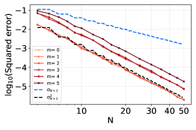
(a) The residual $\|f-\hat{f}_{\mathrm{LS},\bm{x}}\|_{\omega}^{2}$ vs. $N$ ($s=1$).

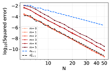
(b) The residual $\|f-\hat{f}_{\mathrm{LS},\bm{x}}\|_{\omega}^{2}$ vs. $N$ ($s=2$).

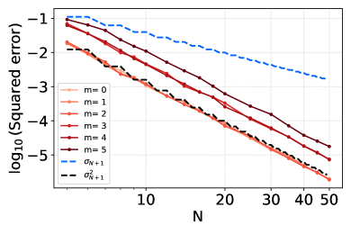
(c) The residual $\|f-\hat{f}_{\mathrm{OKA},\bm{x}}\|_{\omega}^{2}$ vs. $N$ ($s=1$).

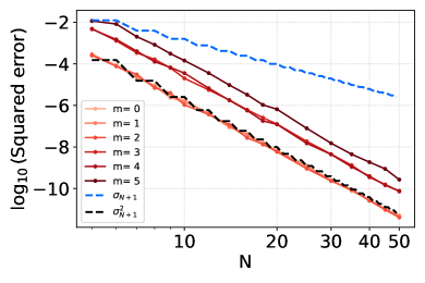
(d) The residual $\|f-\hat{f}_{\mathrm{OKA},\bm{x}}\|_{\omega}^{2}$ vs. $N$ ($s=2$).

Figure 2: The reconstruction error for $f=e_{m}^{\mathcal{F}}$, when $\operatorname{\mathcal{F}}$ is the periodic Sobolev space of order $s\in\{1,2\}$.

Now, we move to another experiment, and consider $f$ to be a random function

$$f=\sum\limits_{m=1}^{M}\xi_{m}e_{m}^{\operatorname{\mathcal{F}}},$$ (96)

where $M\in\mathbb{N}^{*}$ and the $\xi_{m}$ are i.i.d. standard Gaussians. In other words, $f$ is a random element of the eigenspace $\mathcal{E}^{\operatorname{\mathcal{F}}}_{M}$. Figure 3a and Figure 3b show log-log plots of $\|f-\hat{f}_{\mathrm{LS},\bm{x}}\|_{\omega}^{2}$ w.r.t. $N$, averaged over 50 independent DPP samples, and for a set of $50$ functions $f$ sampled according to (96), when $\operatorname{\mathcal{F}}$ is the periodic Sobolev spaces of order $s=1$. To be clear, for every function $f$ we use different DPP samples. We observe that the empirical convergence rate scales as $\mathcal{O}(\sigma_{N+1}^{2})$, which is slightly faster than $\mathcal{O}(\sum_{m\geq N+1}\sigma^{2}_{m})$. Again, this fast convergence is also observed for the kernel-based interpolant $\hat{f}_{\mathrm{OKA},\bm{x}}$, as shown in Figure 3c and Figure 3d.

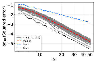
(a) The residual $\|f-\hat{f}_{\mathrm{LS},\bm{x}}\|_{\omega}^{2}$ vs. $N$ for $M=10$.

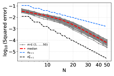
(b) The residual $\|f-\hat{f}_{\mathrm{LS},\bm{x}}\|_{\omega}^{2}$ vs. $N$ for $M=20$.

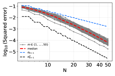
(c) The residual $\|f-\hat{f}_{\mathrm{OKA},\bm{x}}\|_{\omega}^{2}$ vs. $N$ for $M=10$.

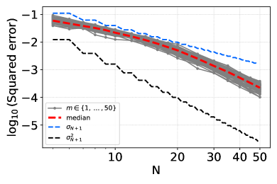
(d) The residual $\|f-\hat{f}_{\mathrm{OKA},\bm{x}}\|_{\omega}^{2}$ vs. $N$ for $M=20$.

Figure 3: The reconstruction error for $10$ samples of $f$ from the distribution defined by (96) when $\operatorname{\mathcal{F}}$ is the periodic Sobolev space of order $s=1$.

4.2 An RKHS with a rotation-invariant kernel on the hypersphere

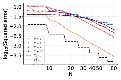
(a) The residual $\|f-\hat{f}_{\mathrm{LS},\bm{x}}\|_{\omega}^{2}$ vs. $N$ ($s=1$).

(b) The residual $\|f-\hat{f}_{\mathrm{LS},\bm{x}}\|_{\omega}^{2}$ vs. $N$ ($s=2$).

Figure 4: The reconstruction error for $f=e_{m}^{\mathcal{F}}$, when $\operatorname{\mathcal{F}}$ is the periodic Sobolev space of order $s\in\{1,2\}$ in the hypersphere $\mathbb{S}^{d-1}$ where $d=3$.

The RKHS framework allow treating high-dimensional and/or non-Euclidean domains. In this section, we illustrate the superconvergence phenomenon of Theorem 1 on a hypersphere.

The definition of a positive definite kernel on a hypersphere dates back to the seminal work of Schoenberg (1942). A kernel $k:\mathbb{S}^{d-1}\times\mathbb{S}^{d-1}\rightarrow\mathbb{R}$ is said to be a dot-product kernel if there exists a function $\varphi:[-1,1]\rightarrow\mathbb{R}$ such that $k(x,y)=\varphi(\langle x,y\rangle)$ for $x,y\in\mathbb{S}^{d-1}$. This defines a large class of rotation-invariant kernels on $\mathbb{S}^{d-1}$. Moreover, the integration operator $\bm{\Sigma}$ associated to a dot-product kernel, when $\mathbb{S}^{d-1}$ is equipped with the uniform measure, decomposes in the basis of spherical harmonics, and Mercer’s decomposition holds in the form

$$k(x,y)=\sum\limits_{\ell=0}^{+\infty}\sigma_{\ell}\sum\limits_{k=1}^{N(d,\ell)}Y_{\ell,k}(x)Y_{\ell,k}(y),$$ (97)

where for $\ell\in\mathbb{N}$, $\{Y_{\ell,k}:\mathbb{S}^{d-1}\rightarrow\mathbb{R},k=1,\dots,N(d,\ell)\}$ is the basis of spherical harmonics of exact degree $\ell$ and $N(d,\ell):=(2\ell+d-1)\Gamma(\ell+d-1)/\big{(}\Gamma(d)\Gamma(\ell+1)\big{)}$; see (Groemer, 1996). The exact expression of $\sigma_{m}$ or the eigenvalue decay may be found in (Cui and Freeden, 1997; Smola et al., 2000; Bach, 2017b; Azevedo and Menegatto, 2014; Scetbon and Harchaoui, 2021).

In order to illustrate the superconvergence phenomenon of Theorem 1,we consider the kernel obtained by taking $d=3$ and $\sigma_{\ell}=(1+\ell)^{-2s}$ in (97). The corresponding RKHS is akin to a Sobolev space of order $s$; an element of $\mathcal{F}$ is a function $f$ defined on $\mathbb{S}^{d-1}$, which has a derivative of order $s$ in the sense of distributions such that $f^{(s)}\in\mathbb{L}_{2}(\omega)$ (Hesse, 2006).

Figure 4a and Figure 4b show log-log plots of $\|f-\hat{f}_{\mathrm{LS},\bm{x}}\|_{\omega}^{2}$ when $f=e_{m}^{\operatorname{\mathcal{F}}}$ with $m\in\{1,10,20,30\}$ w.r.t. $N$, averaged over 50 independent DPP samples, for $s=1$ and $s=2$ respectively. Again, we observe that the expected squared residual converges to $0$ at the same rate as $\sigma_{N+1}^{2}=\mathcal{O}(N^{-4s})$, which is slightly faster than the rate of convergence predicted by Theorem 1 of $\sum_{m\geq N+1}\sigma^{2}_{m}=\mathcal{O}(N^{1-4s})$. Moreover, the superconvergence regime corresponds to $N\geq m$, as predicted by Theorem 1.

4.3 The RKHS spanned by the uni-dimensional PSWFs

In this section, we compare DPP-based sampling with i.i.d. Christoffel sampling in the classical setting of band-limited signals.

Let now $\mathcal{X}=[-T/2,T/2]$ equipped with $\omega$ the uniform measure, and let $F>0$. Consider the so-called Sinc kernel

$$k_{F}(x,y):=\mathrm{Sinc}(F(x-y))=\frac{\sin(F(x-y))}{F(x-y)}.$$ (98)

This kernel defines an RKHS that corresponds to the space of band-limited functions restricted to the interval $\mathcal{X}$. Slepian, Landau, and Pollak proved that the eigenfunctions of the integration operator $\bm{\Sigma}$ associated to (98) and the measure $\omega$ satisfy a differential equation known in physics as the prolate spheroidal wave equation (PSW; Slepian and Pollak, 1961). Since this seminal work, the eponymous functions were subject to extensive research. In particular, a detailed description of the eigenfunctions was carried out in (Osipov, 2013; Bonami and Karoui, 2014; Osipov and Rokhlin, 2012). In particular, these functions were shown to be well represented in the orthonormal basis defined by the Legendre polynomials (Boyd, 2005; Osipov et al., 2013).

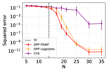
(a) The residual $\|f-\hat{f}_{\mathrm{OKA},\bm{x}}\|_{\omega}^{2}$ vs. $N$ ($m=1$).

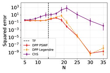
(b) The residual $\|f-\hat{f}_{\mathrm{OKA},\bm{x}}\|_{\omega}^{2}$ vs. $N$ ($m=2$).

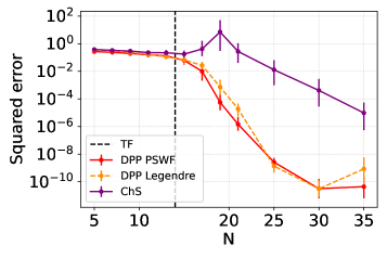
(c) The residual $\|f-\hat{f}_{\mathrm{OKA},\bm{x}}\|_{\omega}^{2}$ vs. $N$ ($m=3$).

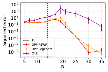
(d) The residual $\|f-\hat{f}_{\mathrm{OKA},\bm{x}}\|_{\omega}^{2}$ vs. $N$ ($m=4$).

Figure 5: The reconstruction error for $f=e_{m}^{\mathcal{F}}$ in the RKHS associated to the Sinc kernel.

The asymptotics of the eigenvalues $(\sigma_{m})$ of $\bm{\Sigma}$ in the limit $c:=TF\rightarrow+\infty$ were investigated too (Landau and Widom, 1980): for $\epsilon>0$, in this asymptotic regime, $\bm{\Sigma}$ has approximately $TF$ eigenvalues in the interval $[1-\epsilon,1]$, $\mathcal{O}(\log(TF)\log(1/\epsilon))$ eigenvalues in the interval $[\epsilon,1-\epsilon]$, and the remaining eigenvalues decrease to $0$ at an exponential rate.

In this set of experiments, we study the influence of the design $\bm{x}$ on the convergence of $\hat{f}_{\mathrm{OKA},\bm{x}}$ to $f$ with respect to the norm $\|.\|_{\omega}$. We compare the following random designs: (i) the projection DPP defined in Section 2.3.2 associated to the first PSW functions (DPP-PSWF), (ii) the projection DPP associated to the first normalized Legendre polynomials (DPP-Legendre), and (iii) i.i.d. Christoffel sampling (ChS). Figure 5 shows log-log plots of $\|f-\hat{f}_{\mathrm{OKA},\bm{x}}\|_{\omega}^{2}$ w.r.t. $N$, when $f=e_{m}^{\operatorname{\mathcal{F}}}$ with $m\in\{1,2,3\}$, averaged over 50 independent samples of each of the three distributions. We observe that both DPP-PSWF and DPP-Legendre significantly improve over Christoffel sampling. Moreover, the expected squared residual $\|f-\hat{f}_{\mathrm{OKA},\bm{x}}\|_{\omega}^{2}$ under the two DPPs converges to $0$ at an exponential rate when $N\geq TF$: we take $T=2$ and $F=7$ so that $TF=14$, which corresponds to the asymptotics described in (Landau and Widom, 1980).

5 Discussion and open questions

In this section, we give some high-level comments and discuss possible extensions of our results.

First, we insist that generating different random designs requires access to different quantities. Christoffel sampling in general will require rejection sampling. One should thus be able to evaluate the density $x\mapsto\sum_{m=1}^{N}e_{m}(x)^{2}/N$, as well as find a suitable proposal. The study of the ‘shape’ of the Christoffel function is thus crucial for sampling, and is an active topic of research (Pauwels et al., 2018; Avron et al., 2019; Dolbeault and Cohen, 2022b). A good sampler for the Christoffel function is also relevant to simulate the DPP of Equation 29, as the p.d.f. of Christoffel sampling can be used as a proposal distribution when sampling the sequential conditionals of the HKPV algorithm (Hough et al., 2006); see (Gautier et al., 2019). When the p.d.f. of Christoffel sampling cannot be evaluated, one can still resort to continuous volume sampling. Indeed, while the only known exact sampling algorithm for CVS still relies on possibly hard-to-evaluate projection kernels, there are approximate samplers that leverage the fact that evaluating the p.d.f. of CVS in Equation 31 only requires evaluating the RKHS kernel $k$. In particular, Rezaei and Gharan (2019) have studied a natural Markov chain Monte Carlo sampler, whose mixing time scales as $\mathcal{O}(N^{5}\log(N))$. Interestingly, each iteration of their Markov chain requires a rejection sampling step, the expected number of rejections is shown to be $\mathcal{O}(1/\sum_{m\geq N+1}\sigma_{m})$. In other words, the smoother the kernel, the harder it is to run the MCMC algorithm. It would be interesting to investigate whether alternative MCMC algorithms can circumvent this ‘smoothness curse’.

Second, we comment on the instance optimal property (IOP), which motivated the introduction of Christoffel sampling (Cohen and Migliorati, 2017). In particular, it was proven that for some variants of the empirical least-squares approximation, the IOP holds when the sampling budget is as low as $\mathcal{O}(M\log(M))$. These variants essentially exclude configurations of nodes $\bm{x}$ for which the Gramian matrix $\bm{G}_{q,\bm{x}}$, defined in the end of Section 2.2.2, is ill-conditioned. Similarly, determinantal sampling implicitly favors configurations of nodes $\bm{x}$ so that $\operatorname{Det}\bm{G}_{q,\bm{x}}$ is large. Moreover, Proposition 4 shows that the IOP holds under a suitable projection DPP, with a minimum sampling budget $N\geq M$. The price to pay is the constant $M+1$ in the IOP. Now, when $N=M$, this constant is $N+1$, which actually improves upon the constant $N^{2}+1$ proven in (Chkifa and Dolbeault, 2023) for an algorithm based on the so-called effective resistances. The latter algorithm generates randomized configurations $\bm{x}$ in a greedy fashion so that the ‘redundancy’ of sampling is reduced.

Third, we might seek approximation schemes that are optimal in some worst-case sense, rather than looking for ones that satisfy the IOP. This is the approach adopted in (Krieg and Ullrich, 2021; Dolbeault et al., 2023), for instance, where the authors investigate the sampling numbers

$$g_{N}:=\inf\limits_{\begin{subarray}{c}x_{1},\dots,x_{N}\in\mathcal{X}\\ \varphi_{1},\dots,\varphi_{N}\in\mathbb{L}_{2}(\omega)\end{subarray}}\sup\limits_{\begin{subarray}{c}f\in\mathcal{F}\\ \|f\|_{\mathcal{F}}\leq 1\end{subarray}}\|f-\sum\limits_{i=1}^{N}f(x_{i})\varphi_{i}\|_{\omega}.$$ (99)

The sampling numbers measure the complexity of the simultaneous recovery of all functions in the unit ball of $\mathcal{F}$. A consequence of the work of Dolbeault et al. (2023) is that there is a universal constant $c\in\mathbb{N}^{*}$ such that $g_{cN}=\mathcal{O}(\sigma_{N+1})$ under assumptions on the decay of $(\sigma_{m})$; see also (Krieg and Ullrich, 2021). Our Corollary 1 matches this fast rate for the worst-case expected error, but it would be interesting to switch expectation and supremum here, and investigate the expected worst-case approximation error. Such a worst-case optimality would further connect to a string of results on the completeness of DPPs (Lyons, 2003; Ghosh, 2015; Bufetov et al., 2021), which look for conditions under which a sample $\bm{x}$ from a DPP is a uniqueness set in the sense that two elements of $\mathcal{F}$ that coincide on $\bm{x}$ are equal.

6 Conclusion

In this article, we studied various finite-dimensional approximations for functions living in an RKHS, based on a finite number of repulsive nodes defined by RKHS-adapted determinantal distributions. Our results give convergence guarantees in $L^{2}$ norm for any function living in the RKHS. They are stronger than those of previous works on determinantal sampling that give convergence guarantees in RKHS norm for functions living in a strict subspace of the RKHS. In particular, we have shown that the mean square error of the least-squares approximation converges to zero at a rate that depends on the eigenvalues of the Mercer decomposition of the RKHS kernel. Moreover, we show that the convergence rate is faster for functions living in a certain low-dimensional subspace of the RKHS. This result provides insight on how the rate improves with smoothness. Moreover, we have investigated approximations that can be evaluated using only a finite number of evaluations of the target function, unlike the least-squares approximation. In particular, we prove that the instance optimality property holds for a particular transform-based approximation using DPPs, even with a minimal sampling budget. This result shows that determinantal sampling generalizes and improves on i.i.d. sampling from the Christoffel function. The numerical experiments conducted in various domains validate our theoretical results. The numerical performance actually exceeds the expectations, which both illustrates the relevance of the proposed approach and shows that there is still some room to improve of our theoretical results. Finally, we have discussed possible extensions of this work.

References

- Adcock and Cardenas [2020] B. Adcock and J. M. Cardenas. Near-optimal sampling strategies for multivariate function approximation on general domains. SIAM Journal on Mathematics of Data Science, 2(3):607–630, 2020.
- Adcock et al. [2022] B. Adcock, J. M. Cardenas, N. Dexter, and S. Moraga. Towards optimal sampling for learning sparse approximations in high dimensions. In High-Dimensional Optimization and Probability: With a View Towards Data Science, pages 9–77. Springer, 2022.
- Aronszajn [1943] N. Aronszajn. La théorie des noyaux reproduisants et ses applications première partie. In Mathematical Proceedings of the Cambridge Philosophical Society, volume 39, pages 133–153. Cambridge University Press, 1943.
- Aronszajn [1950] N. Aronszajn. Theory of reproducing kernels. Transactions of the American mathematical society, 68(3):337–404, 1950.
- Avron et al. [2019] H. Avron, M. Kapralov, C. Musco, C. Musco, A. Velingker, and A. Zandieh. A universal sampling method for reconstructing signals with simple fourier transforms. In Proceedings of the 51st Annual ACM SIGACT Symposium on Theory of Computing, pages 1051–1063, 2019.
- Azevedo and Menegatto [2014] D. Azevedo and V. A. Menegatto. Sharp estimates for eigenvalues of integral operators generated by dot product kernels on the sphere. Journal of Approximation Theory, 177:57–68, 2014.
- Bach [2017a] F. Bach. On the equivalence between kernel quadrature rules and random feature expansions. The Journal of Machine Learning Research, 18(1):714–751, 2017a.
- Bach [2017b] F. Bach. Breaking the curse of dimensionality with convex neural networks. The Journal of Machine Learning Research, 18(1):629–681, 2017b.
- Bardenet and Hardy [2020] R. Bardenet and A. Hardy. Monte carlo with determinantal point processes. The Annals of Applied Probability, 30(1):368–417, 2020.
- Belhadji [2020] A. Belhadji. Subspace sampling using determinantal point processes. PhD thesis, Centrale Lille Institut, 2020.
- Belhadji [2021] A. Belhadji. An analysis of Ermakov-Zolotukhin quadrature using kernels. Advances in Neural Information Processing Systems, 34:27278–27289, 2021.
- Belhadji et al. [2019] A. Belhadji, R. Bardenet, and P. Chainais. Kernel quadrature with DPPs. In Advances in Neural Information Processing Systems, pages 12907–12917, 2019.
- Belhadji et al. [2020] A. Belhadji, R. Bardenet, and P. Chainais. Kernel interpolation with continuous volume sampling. arXiv preprint arXiv:2002.09677, 2020.
- Berlinet and Thomas-Agnan [2011] A. Berlinet and Ch. Thomas-Agnan. Reproducing kernel Hilbert spaces in probability and statistics. Springer Science & Business Media, 2011.
- Bonami and Karoui [2014] A. Bonami and A. Karoui. Uniform bounds of prolate spheroidal wave functions and eigenvalues decay. Comptes Rendus Mathematique, 352(3):229–234, 2014.
- Bos [1994] L. Bos. Asymptotics for the Christoffel function for Jacobi like weights on a ball in . New Zealand J. Math, 23(99):109, 1994.
- Boyd [2005] J. P. Boyd. Algorithm 840: computation of grid points, quadrature weights and derivatives for spectral element methods using prolate spheroidal wave functions—prolate elements. ACM Transactions on Mathematical Software (TOMS), 31(1):149–165, 2005.
- Brezis [2010] H. Brezis. Functional analysis, Sobolev spaces and partial differential equations. Springer Science & Business Media, 2010.
- Bufetov et al. [2021] A. I. Bufetov, Y. Qiu, and A. Shamov. Kernels of conditional determinantal measures and the Lyons–Peres completeness conjecture. Journal of the European Mathematical Society, 23(5):1477–1519, 2021.
- Butzer and Stens [1992] P. L. Butzer and R. L. Stens. Sampling theory for not necessarily band-limited functions: a historical overview. SIAM review, 34(1):40–53, 1992.
- Campbell [1964] L. Campbell. A comparison of the sampling theorems of Kramer and Whittaker. Journal of the Society for Industrial and Applied Mathematics, 12(1):117–130, 1964.
- Chkifa and Dolbeault [2023] A. Chkifa and M. Dolbeault. Randomized least-squares with minimal oversampling and interpolation in general spaces. arXiv preprint arXiv:2306.07435, 2023.
- Cohen and Migliorati [2017] A. Cohen and G. Migliorati. Optimal weighted least-squares methods. The SMAI journal of computational mathematics, 3:181–203, 2017.
- Cohen et al. [2013] A. Cohen, M. A. Davenport, and D. Leviatan. On the stability and accuracy of least squares approximations. Foundations of computational mathematics, 13:819–834, 2013.
- Cui and Freeden [1997] J. Cui and W. Freeden. Equidistribution on the sphere. SIAM Journal on Scientific Computing, 18(2):595–609, 1997.
- de La Vallée Poussin [1908] Ch.-J. de La Vallée Poussin. Sur la convergence des formules d’interpolation entre ordonnées équidistantes. Hayez, 1908.
- Dolbeault and Cohen [2022a] M. Dolbeault and A. Cohen. Optimal sampling and Christoffel functions on general domains. Constructive Approximation, 56(1):121–163, 2022a.
- Dolbeault and Cohen [2022b] M. Dolbeault and A. Cohen. Optimal pointwise sampling for approximation. Journal of Complexity, 68:101602, 2022b.
- Dolbeault et al. [2023] M. Dolbeault, D. Krieg, and Mario Ullrich. A sharp upper bound for sampling numbers in . Applied and Computational Harmonic Analysis, 63:113–134, 2023.
- Erdős and Turán [1937] P. Erdős and P. Turán. On interpolation i. Annals of mathematics, pages 142–155, 1937.
- Ermakov and Zolotukhin [1960] S. M. Ermakov and V.G. Zolotukhin. Polynomial approximations and the Monte Carlo method. Theory of Probability & Its Applications, 5(4):428–431, 1960.
- Filbir and Mhaskar [2011] F. Filbir and H. N. Mhaskar. Marcinkiewicz–Zygmund measures on manifolds. Journal of Complexity, 27(6):568–596, 2011.
- Gautier et al. [2019] G. Gautier, R. Bardenet, and M. Valko. On two ways to use determinantal point processes for Monte Carlo integration. Advances in Neural Information Processing Systems, 32, 2019.
- Gautschi [2004] W. Gautschi. Orthogonal polynomials: computation and approximation. OUP Oxford, 2004.
- Ghosh [2015] S. Ghosh. Determinantal processes and completeness of random exponentials: the critical case. Probability Theory and Related Fields, 163(3-4):643–665, 2015.
- Gröchenig [1993] K. Gröchenig. A discrete theory of irregular sampling. Linear Algebra and its applications, 193:129–150, 1993.
- Gröchenig [2020] K. Gröchenig. Sampling, Marcinkiewicz–Zygmund inequalities, approximation, and quadrature rules. Journal of Approximation Theory, 257:105455, 2020.
- Groemer [1996] H. Groemer. Geometric applications of Fourier series and spherical harmonics, volume 61. Cambridge University Press, 1996.
- Haberstich et al. [2022] C. Haberstich, A. Nouy, and G. Perrin. Boosted optimal weighted least-squares. Mathematics of Computation, 91(335):1281–1315, 2022.
- Hampton and Doostan [2015] J. Hampton and A. Doostan. Coherence motivated sampling and convergence analysis of least squares polynomial chaos regression. Computer Methods in Applied Mechanics and Engineering, 290:73–97, 2015.
- Hesse [2006] K. Hesse. A lower bound for the worst-case cubature error on spheres of arbitrary dimension. Numerische Mathematik, 103:413–433, 2006.
- Higgins [1985] J. R. Higgins. Five short stories about the cardinal series. Bulletin of the American Mathematical Society, 12(1):45–89, 1985.
- Hough et al. [2006] J. B. Hough, M. Krishnapur, Y. Peres, and B. Virág. Determinantal processes and independence. Probability surveys, 3:206–229, 2006.
- Jerri [1976] A. Jerri. Sampling expansion for Laguerre-L: transforms. J. Res. Nat. Bur. Standards B, 80(3):415–418, 1976.
- Johansson [2005] K. Johansson. Random matrices and determinantal processes. ArXiv Mathematical Physics e-prints, October 2005.
- Kassel and Lévy [2022] A. Kassel and T. Lévy. On the mean projection theorem for determinantal point processes. arXiv preprint arXiv:2203.04628, 2022.
- Koornwinder and Walter [1990] T. H. Koornwinder and G. G. Walter. The finite continuous Jacobi transform and its inverse. Journal of Approximation Theory, 60(1):83–100, 1990.
- Kotel’nikov [2006] V. A. Kotel’nikov. On the transmission capacity of ’ether’ and wire in electric communications. Physics-Uspekhi, 49(7):736–744, 2006.
- Kramer [1959] H. P. Kramer. A generalized sampling theorem. Journal of Mathematics and Physics, 38(1-4):68–72, 1959.
- Krieg [2019] D. Krieg. Optimal monte carlo methods for -approximation. Constructive Approximation, 49(2):385–403, 2019.
- Krieg and Ullrich [2021] D. Krieg and M. Ullrich. Function values are enough for -approximation: Part ii. Journal of Complexity, 66:101569, 2021.
- Kulesza and Taskar [2012] A. Kulesza and B. Taskar. Determinantal point processes for machine learning. Foundations and Trends® in Machine Learning, 5(2–3):123–286, 2012.
- Landau and Widom [1980] H. J. Landau and H. Widom. Eigenvalue distribution of time and frequency limiting. Journal of Mathematical Analysis and Applications, 77(2):469–481, 1980.
- Larkin [1972] F. M. Larkin. Gaussian measure in Hilbert space and applications in numerical analysis. The Rocky Mountain Journal of Mathematics, pages 379–421, 1972.
- Lavancier et al. [2015] F. Lavancier, J. Møller, and E. Rubak. Determinantal point process models and statistical inference. Journal of the Royal Statistical Society: Series B (Statistical Methodology), 77(4):853–877, 2015.
- Lyons [2003] R. Lyons. Determinantal probability measures. Publications Mathématiques de l’IHÉS, 98:167–212, 2003.
- Lyons [2014] R. Lyons. Determinantal probability: basic properties and conjectures. arXiv preprint arXiv:1406.2707, 2014.
- Macchi [1975] O Macchi. The coincidence approach to stochastic point processes. 7:83–122, 03 1975.
- Macchi [2017] O. Macchi. Point processes and coincidences – Contributions to the theory, with applications to statistical optics and optical communication, augmented with a scholion by Suren Poghosyan and Hans Zessin. Walter Warmuth Verlag, 2017.
- Marcus et al. [2015] A. W. Marcus, D. A. Spielman, and N. Srivastava. Interlacing families ii: Mixed characteristic polynomials and the Kadison—Singer problem. Annals of Mathematics, pages 327–350, 2015.
- Muandet et al. [2017] K. Muandet, K. Fukumizu, B. Sriperumbudur, and B. Schölkopf. Kernel mean embedding of distributions: A review and beyond. Foundations and Trends® in Machine Learning, 10(1-2):1–141, 2017.
- Nashed and Walter [1991] M. Z. Nashed and G. G. Walter. General sampling theorems for functions in reproducing kernel hilbert spaces. Mathematics of Control, Signals and Systems, 4(4):363, 1991.
- Nevai [1986] P. Nevai. Géza Freud, orthogonal polynomials and Christoffel functions. a case study. Journal of approximation theory, 48(1):3–167, 1986.
- Novak [1992] E. Novak. Optimal linear randomized methods for linear operators in Hilbert spaces. Journal of Complexity, 8(1):22–36, 1992.
- Ortega-Cerdà and Saludes [2007] J. Ortega-Cerdà and J. Saludes. Marcinkiewicz–Zygmund inequalities. Journal of approximation theory, 145(2):237–252, 2007.
- Osipov [2013] A. Osipov. Certain upper bounds on the eigenvalues associated with prolate spheroidal wave functions. Applied and Computational Harmonic Analysis, 35(2):309–340, 2013.
- Osipov and Rokhlin [2012] A. Osipov and V. Rokhlin. Detailed analysis of prolate quadratures and interpolation formulas. arXiv preprint arXiv:1208.4816, 2012.
- Osipov et al. [2013] A. Osipov, V. Rokhlin, and H. Xiao. Prolate spheroidal wave functions of order zero. Springer Ser. Appl. Math. Sci, 187, 2013.
- Pauwels et al. [2018] E. Pauwels, F. Bach, and J.-P. Vert. Relating leverage scores and density using regularized christoffel functions. Advances in Neural Information Processing Systems, 31, 2018.
- Rezaei and Gharan [2019] A. Rezaei and S. O. Gharan. A polynomial time MCMC method for sampling from continuous determinantal point processes. In International Conference on Machine Learning, pages 5438–5447, 2019.
- Scetbon and Harchaoui [2021] M. Scetbon and Z. Harchaoui. A spectral analysis of dot-product kernels. In International conference on artificial intelligence and statistics, pages 3394–3402. PMLR, 2021.
- Schaback [2018] R. Schaback. Superconvergence of kernel-based interpolation. Journal of Approximation Theory, 235:1–19, 2018.
- Schaback and Wendland [2006] R. Schaback and H. Wendland. Kernel techniques: from machine learning to meshless methods. Acta numerica, 15:543–639, 2006.
- Schoenberg [1942] I. J. Schoenberg. Positive definite functions on spheres. Duke Mathematical Journal, 9(1):96 – 108, 1942. doi: 10.1215/S0012-7094-42-00908-6.
- Shannon [1949] C. E. Shannon. Communication in the presence of noise. Proceedings of the IRE, 37(1):10–21, 1949.
- Slepian and Pollak [1961] D. Slepian and H. O. Pollak. Prolate spheroidal wave functions, fourier analysis and uncertainty—i. Bell System Technical Journal, 40(1):43–63, 1961.
- Sloan [1995] I. H. Sloan. Polynomial interpolation and hyperinterpolation over general regions. Journal of Approximation Theory, 83(2):238–254, 1995.
- Smola et al. [2000] A. Smola, Z. Ovári, and R. C. Williamson. Regularization with dot-product kernels. Advances in neural information processing systems, 13, 2000.
- Steinwart and Scovel [2012] I. Steinwart and C. Scovel. Mercer’s theorem on general domains: on the interaction between measures, kernels, and RKHSs. Constructive Approximation, 35(3):363–417, 2012.
- Totik [2000] V. Totik. Asymptotics for Christoffel functions for general measures on the real line. Journal d’Analyse Mathématique, 81(1):283–303, 2000.
- Wahba [1990] G. Wahba. Spline Models for Observational Data, volume 59. SIAM, 1990.
- Wasilkowski and Woźniakowski [2007] G. W. Wasilkowski and H. Woźniakowski. The power of standard information for multivariate approximation in the randomized setting. Mathematics of computation, 76(258):965–988, 2007.
- Wendland [2004] H. Wendland. Scattered Data Approximation. Cambridge University Press, 2004.
- Whittaker [1928] J. M. Whittaker. The “Fourier” theory of the cardinal function. Proceedings of the Edinburgh Mathematical Society, 1(3):169–176, 1928.
- Xu [1996] Y. Xu. Asymptotics for orthogonal polynomials and Christoffel functions on a ball. Methods and Applications of Analysis, 3(2):257–272, 1996.
- Yao [1967] K. Yao. Applications of reproducing kernel Hilbert spaces–bandlimited signal models. Information and Control, 11(4):429–444, 1967.