Sub-network Discovery and Soft-masking for Continual Learning
of Mixed Tasks

Abstract

Continual learning (CL) has two main objectives: preventing catastrophic forgetting (CF) and encouraging knowledge transfer (KT). The existing literature mainly focused on overcoming CF. Some work has also been done on KT when the tasks are similar. To our knowledge, only one method has been proposed to learn a sequence of mixed tasks. However, these techniques still suffer from CF and/or limited KT. This paper proposes a new CL method to achieve both. It overcomes CF by isolating the knowledge of each task via discovering a sub-network for it. A soft-masking mechanism is also proposed to preserve the previous knowledge and to enable the new task to leverage the past knowledge to achieve KT. Experiments using classification, generation, information extraction, and their mixture (i.e., heterogeneous tasks) show that the proposed method consistently outperforms strong baselines.

1 Introduction

One of the overarching goals of AI is to develop agents that can continually learn diverse tasks. Toward this goal, continual learning (CL) has been proposed, which incrementally learns a sequence of tasks, 1, …., $T$ Chen and Liu (2018). Once a task $t$ is learned, its training data $D_{t}$ (at least a majority of it) is no longer accessible. This paper studies CL of NLP tasks Ke and Liu (2022), where a task is an end-task, e.g., text classification, summarization or information extraction, in the popular setting of task-incremental learning (TIL), in which the task-id is given in both training and testing.

Ideally, CL should (1) overcome catastrophic forgetting (CF), i.e., it should not degrade the performance of previously learned tasks; (2) encourage knowledge transfer (KT) across tasks, i.e., the learning of a task should be able to leverage the knowledge learned from previous tasks; and (3) be able to learn a mixed sequence of similar and dissimilar tasks and achieve both (1) and (2).

Most existing approaches for TIL address one of the three to the detriment of the others. For example, HAT Serrà et al. (2018) and SupSup (Wortsman et al., 2020) can overcome CF by isolating the parameters of each task, which makes KT difficult. CUBER (Lin et al., 2022a) and DAS Ke et al. (2023) can achieve KT by allowing some updates to existing knowledge, which causes CF. ProgressiveNet Rusu et al. (2016) assures no CF by fixing all the learned parameters and expanding the network, but it limits KT. To our knowledge, CAT (Ke et al., 2020) is the only system that tries to have all three capabilities. However, it still suffers from CF due to its weak task similarity detection (for KT) and parameter sharing across dissimilar tasks.

This paper takes a major step to achieve all three objectives without suffering from the above drawbacks. The proposed system is called TSS (TIL based on Sub-network discovery and Soft-masking). TSS performs two functions, (A) sub-network discovery with soft-masking and (B) importance computation, to learn a mixed sequence, where some tasks may be similar (which enable KT) and some may be dissimilar.

Given a fixed and randomly initialized backbone network $N$, function (A) finds a separate sub-network as the model for each task. A sub-network is indicated by a set of binary gates, one for each parameter of $N$, specifying whether the corresponding parameter in $N$ should be in the sub-network for the task. In training, $N$ is fixed and the binary gates are obtained by learning a set of positive and real-valued popup scores (one for each parameter of $N$) and then applying a threshold on the popup scores. In other words, we convert the network training into the popup scores training. Only the binary gates (1’s) obtained from the trained popup scores are stored for each task as its model. Thus, there is no interference across tasks to cause CF as the backbone network is fixed.

This sub-network discovery is effective for overcoming CF, but it prevents KT if the popup scores of each task are independently trained with no sharing across tasks. A naive way to share knowledge is to initialize the popup scores of the new task $t$ with the trained popup scores of the previous task $t-1$. However, this is problematic for a mixed sequence of similar and dissimilar tasks because the training of task $t$ can only leverage the knowledge from the $(t-1)$th task. This can cause negative transfer if task $t-1$ is dissimilar to task $t$. To address this, we propose a soft-masking mechanism to make the initialization of popup scores for the new task contain the learned knowledge from all previous tasks so that the new task training can leverage the knowledge of all previous similar tasks. This is a key novelty of our approach. It is achieved by reducing (called “soft-masking”) the gradient corresponding to the subset of popup scores that are important to previous tasks ($1...t-1$) in training the current task $t$ so that the previously learned knowledge is well protected. In this way, the trained popup scores for task $t$, which will be used as the initialization for the next task, contain not only the knowledge for task $t$ but also the knowledge from all previous tasks. This is critical for learning a mixed sequence of similar and dissimilar tasks because the system does not know a priori which tasks’ knowledge can be transferred to the current task. Note that soft-masking is only applied in backward propagation to preserve old knowledge. In the forward pass, the training can still use all popup scores corresponding to all parameters of the backbone network. Additionally, soft-masking reduces the gradient instead of fully blocking the gradient, which gives the model the flexibility to adjust any popup scores when training the current task $t$, which further encourages KT.

The question is how to decide the important popup scores for each task. This is done by (B), which computes the importance of the popup scores after training a task. The importance is a number between 0 and 1. After training popup scores for a task, we input the training data again to compute the importance of each popup score for the task based on its gradient. We save the accumulated importance over all previous tasks to keep track of the important popup scores so far. The accumulated importance (within 0 and 1; thus “soft”) is used to guide soft-masking in (A) in training a new task.

This paper makes three key contributions.

1. It studies an important but under-studied problem of continually learning a mixed sequence, where some tasks may be similar and some may be dissimilar. Existing CL methods suffer from either CF or limited KT in this scenario.

2. It proposes a novel method TSS consisting of sub-network discovery with soft-masking and importance computation to prevent CF and to encourage KT for a mixed sequence of tasks.

3. It evaluates TSS using datasets consisting of classification, generation and information extraction tasks and their mixture. The results demonstrate the effectiveness of TSS.

2 Related Work

Forgetting prevention in continual learning (CL). There are four main families of approaches:

(1) Regularization-based approaches (Kirkpatrick et al., 2016; Lee et al., 2017; Seff et al., 2017; Zenke et al., 2017; Rusu et al., 2016) add a regularization in the loss to penalize changes to parameters that are important to previous tasks. Gradient projection (Zeng et al., 2019) ensures the gradient updates occur in the orthogonal direction to the input of old tasks and in trust region (Lin et al., 2022a, b) TSS uses no regularization.

(2) Replay-based approaches (Rebuffi et al., 2017; Lopez-Paz and Ranzato, 2017; Chaudhry et al., 2019; Wang et al., 2020) retain some training data of old tasks and use them in learning a new task. The methods in (Shin et al., 2017; Kamra et al., 2017; Rostami et al., 2019; He and Jaeger, 2018) learn data generators and generate old task data for learning a new task. These are clearly different from TSS as it uses no any replay data.

(3) Parameter isolation (Serrà et al., 2018; Ke et al., 2020, 2021a; Mallya and Lazebnik, 2018; Fernando et al., 2017; Wortsman et al., 2020) learns and masks a dedicated sub-network for each task, but has limited KT. TSS leverages this approach to isolate knowledge for different tasks, but enables KT by using a soft-mask mechanism to preserve the learned knowledge and uses the old knowledge as the initialization for learning the new task.

(4) Parameter isolation plus out-of-distribution (OOD) detection is a new and theoretical grounded approach Kim et al. (2022, 2023). It is mainly used for class-incremental learning (CIL). The main idea is to use a parameter isolation approach for task incremental learning (TIL) to overcome CF and the model for each task is an OOD detection model. During inference, the system performs both task-id prediction and within-task prediction for CIL classification. However, our work is about TIL.

Knowledge transfer in CL. There are two main approaches for KT: (1) replay-based Huang et al. (2021); Wang et al. (2021, 2020); de Masson d’Autume et al. (2019); Zhu et al. (2022); Yin et al. (2022), which use replay data to help the transfer. TSS is replay-free. (2) similarity-based, which uses task similarities using features Ke et al. (2021a, b, 2020); Wang et al. (2022); Zhang et al. (2022) or gradients Lin et al. (2022a). However, these methods are not always reliable, which results in CF. CAT (Ke et al., 2020) considers a mixed sequence of tasks by first detecting previous tasks that are similar to the current task and then opening the masks of these tasks so that the new task learning can modify their parameters to achieve KT. However, this causes CF for dissimilar tasks that share parameters with those similar tasks. DAS Ke et al. (2023) encourages KT by allowing previous knowledge updates based on importance, but this also causes CF because previous parameters is changeable and there is no easy way to separate the parameters that are used for different tasks. In contrast, TSS does not require any explicit similarity detection but finds sub-network for each task to guarantee no CF. Its soft-masks allow the initialization contains all previously learned knowledge and thus encourage KT to the new task. Konishi et al. (2023) recently proposed a parameter-level soft-masking method using AlexNet as the backbone. The method has difficulties working with more complex architectures. Our soft-masks are set on the popup scores rather than network parameters and our approach is based on sub-network discovery and knowledge sharing.

Network pruning as importance computation. It is known that many parameters in a neural network are redundant and can be pruned (Li et al., 2021; Lai et al., 2021; Chen et al., 2020; Lin et al., 2020; Gao et al., 2021; Voita et al., 2019). For Transformer, one can prune the attention head (Michel et al., 2019; Voita et al., 2019; McCarley et al., 2019) and sub-layers (Fan et al., 2020; Sajjad et al., 2020). However, these methods are not directly applicable to us as we need to compute the importance of each popup score instead of each parameter in the network. We use the importance as soft-masks to leverage all existing sub-networks for KT rather than to compress the LM.

3 Proposed TSS Technique

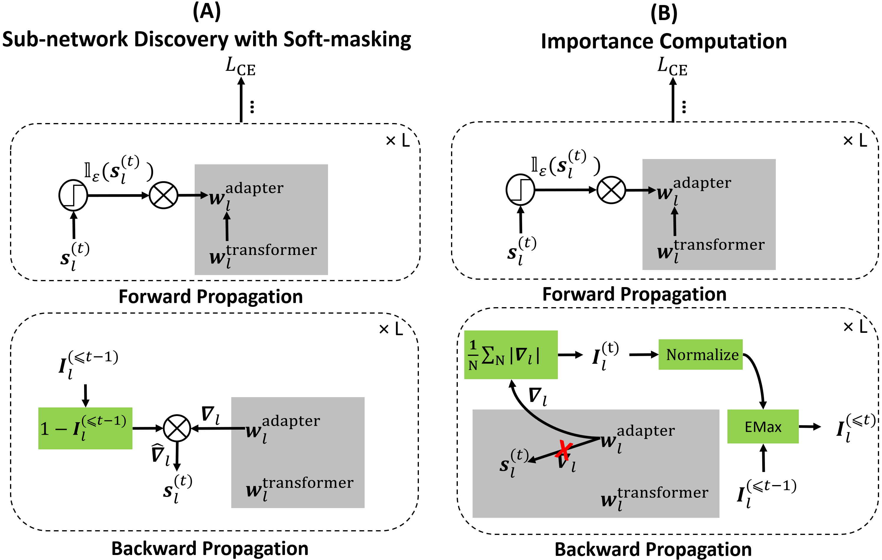
Figure 1: Illustration of TSS in training task $t$. The detailed description is in Sec. 3. The grey boxes indicate that the parameters of the adapters and backbone language model (LM) are all frozen. The only trainable parameters are the popup scores $\bm{s}_{l}^{(t)}$. In (A) sub-network discovery with soft-masking (Sec. 3.1.1), we remove the step function in the backward propagation to reflect the straight-through estimator in Eq. LABEL:eq.optimize, where the gradient “skips” the step function as if it is an identity function. The original gradient for popup scores, $\nabla_{l}$, is not directly used to update the popup scores but soft-masked based on the accumulated importance (Sec. 3.1.2). In (B) Importance Computation (Sec. 3.2), the red cross in backward propagation indicates that the gradient is not used to update the popup scores $\bm{s}_{l}^{(t)}$ but only to compute the importance.

TSS is designed for both CF prevention and forward KT. Figure 1 gives an overview of TSS. The backbone network consists of the transformer and adapters, which are indicated by the transformer parameters $\bm{w}_{l}^{\text{transformer}}$ of layer $l$ and by the parameters of adapter $\bm{w}_{l}^{\text{adapter}}$ of layer $l$ respectively (see the grey boxes). Note again that these are fixed in the entire learning process. On the left, we show the forward pass and backward propagation of (A) sub-network discovery with soft-masking (Sec. 3.1). In the forward pass, a set of learnable popup scores $\bm{s}_{l}^{(t)}$ are initialized (Sec. 3.1.2) and fed into a step function. The output of the step function is a set of binary gates $\bm{g}_{l}^{(t)}$ that element-wise multiply ($\otimes$) with the parameters of the adapter of the backbone network ($\bm{w}_{l}^{\text{adapter}}$). As a result, the binary gates indicate a sub-network for task $t$ within the $\bm{w}_{l}^{\text{adapter}}$ (Sec. 3.1.1). In the backward propagation (Sec. 3.1.2), we first accumulate the importance of popup scores for all previous tasks by normalization and element-wise maximum (“EMax”). The accumulated importance $\bm{I}_{l}^{(\leq t-1)}$ is converted into soft-mask by the operation $1-\bm{I}_{l}^{(\leq t-1)}$. This soft-mask is then element-wise multiplied with the original gradient of the popup scores $\bm{s}_{l}^{(t)}$ in layer $l$, $\nabla_{l}$ (computed by straight-through estimator in Eq. LABEL:eq.optimize). The soft-masked gradient, $\hat{\nabla}_{l}$, is the final gradient that is used to optimize the popup scores $\bm{s}_{l}^{(t)}$. Since the important popup scores have lower gradients in $\hat{\nabla}_{l}$, the popup scores that are important to previous tasks are preserved and are used to initialize the new task to encourage KT (not shown in Figure 1).

After (A), we show (B) importance computation (Sec. 3.2). The forward pass is the same as (A). However, in backward propagation, the gradient of popup scores, $\nabla_{l}$, is not used to update anything (red cross in the arrow) but computes the importance using its absolute average value, $\frac{1}{N}\sum_{n=1}^{N}|\nabla_{l}|$. The resulting importance of task $t$ in layer $l$, $\bm{I}_{l}^{(t)}$, is saved for (A) in learning the next task. The following sub-sections present each function and step in detail.

3.1 Sub-network Discovery and Soft-masking

Sub-network discovery finds a sub-network (represented as binary gates) for the current task, which is saved to overcome CF. It relies on the training of popup scores and its training also involves soft-masking to encourage knowledge transfer. In this section, we will present how we discover the sub-network via learning popup scores and how we encourage knowledge transfer (KT) via soft-masking.

3.1.1 From Popup Scores to Sub-network

Since the pre-trained language model (LM) contains useful general knowledge, we fix and use the full LM. The sub-network discovery is only done on adapters Houlsby et al. (2019), which are inserted into each layer of the LM. Note again that throughout the training process, both the adapters (randomly initialized) and backbone LM are fixed.

We now define a set of learnable popup scores $\bm{s}_{l}^{(t)}$ for layer $l$ for task $t$. It has the same size as the parameters of the adapters $w^{\text{adapter}}_{l}$ (which is fixed throughout learning). In the forward pass, $\bm{s}_{l}^{(t)}$ is constantly thresholded,

$$\bm{g}^{(t)}_{l}=\mathbbm{1}_{\epsilon}(\bm{s}^{(t)}_{l}),\vspace{-1mm}$$ (1)

where $\mathbbm{1}$ is a step function that outputs 1 for the scores that are larger than the threshold $\epsilon$ (a hyper-parameter). Since the gate $\bm{g}^{(t)}_{l}$ is always binary, it can naturally indicate a sub-network within the parameters of the fixed adapter, $\bm{w}_{l}^{\text{adapter}}$, by element-wise multiplication,

$$\hat{\bm{w}}_{l}^{\text{adapter}}=\bm{w}_{l}^{\text{adapter}}\otimes\bm{g}^{(t)}_{l},\vspace{-1mm}$$ (2)

where $\otimes$ is element-wise multiplication. $\hat{\bm{w}}_{l}^{adapter}$ indicates the selected parameters in the adapter that form the discovered sub-network.

Training the popup scores. $\bm{s}_{l}^{(t)}$ cannot be directly optimized because the derivative of its threshold-based step functions is zero. Then nothing can be learned. To solve the problem we use straight-through estimators Bengio et al. (2013). Specifically, we ignore the derivative of the threshold function and pass on the incoming gradient as if the threshold function was an identity function. Consequently, for each parameter $s_{i,j}^{(t)}$ in $\bm{s}_{l}^{(t)}$, it is updated as follows,

$$\begin{split}&\bm{s}_{l}^{(t)}=\bm{s}_{l}^{(t)}-\alpha\nabla_{l};\\ &\nabla_{l}=\frac{\partial\mathcal{L}}{\partial s_{i,j}^{(t)}}=\frac{\partial\mathcal{L}}{\partial\mathcal{I}_{j}}\frac{\partial\mathcal{I}_{j}}{\partial s_{i,j}^{(t)}}=\frac{\partial\mathcal{L}}{\partial\mathcal{I}_{j}}w_{i,j}\mathcal{O}_{i},\end{split}$$ (3)

where $\mathcal{I}_{j}$ and $\mathcal{O}_{i}$ are the input and output of neurons $i$ and $j$. $\nabla_{l}$ is the gradients on the popup scores $\bm{s}_{l}^{(t)}$ and $\alpha$ is the learning rate. After training, the binary gate, $\bm{g}_{l}^{(t)}$, is saved (taking only 1-bit per element). Since $\bm{g}_{l}^{(t)}$ is saved, and all the backbone parameters are fixed (including the adapter’s and backbone LM’s), TSS does not suffer from forgetting of the previously learned knowledge.

3.1.2 Preserving Previous Knowledge for New Task Initialization

While the sub-network discovery in Sec. 3.1.1 can help prevent forgetting (CF), it does not do knowledge transfer (KT). As discussed earlier, the naive way for KT is to initialize the popup scores $\bm{s}_{l}^{(t)}$ for the new task $t$ with the learned scores $\bm{s}_{l}^{(t-1)}$ for task $t-1$. However, $\bm{s}_{l}^{(t-1)}$ contains only the knowledge from task $t-1$, but we have no idea whether any knowledge from task $t-1$ can be transferred to task $t$ because tasks $t$ and $t-1$ may be entirely different. To address this, we preserve the learned knowledge from all previous tasks from 1 to $t-1$ in $\bm{s}_{l}^{(t-1)}$. In this way, task $t$ can leverage all previously learned knowledge for KT.

To make the preservation possible, inspired by Ke et al. (2023), we propose a soft-masking mechanism based on the importance of each popup score to all previous tasks. We compute the importance in Sec. 3.2. For now, we assume that we already have the set of importance value $\{\bm{I}^{(k)}_{l}\}_{k=1}^{t-1}$ for $\bm{s}_{l}^{(k)}$ for each previously learned task $k$. The preservation is achieved by soft-masking the learning based on the accumulated importance as follows:

Accumulating importance. We accumulate the importance after task $t-1$ is learned via element-wise max (EMax),

$$\bm{I}_{l}^{(\leq t-1)}=\text{EMax}(\{\bm{I}_{l}^{(t-1)},\bm{I}^{(\leq t-2)}_{l}\}),$$ (4)

where $\bm{I}^{(\leq t-2)}_{l}$ refers to the previously accumulated importance at task $t-2$. We do not need to save all $\{\bm{I}^{(k)}_{l}\}_{k=1}^{t\text{-1}}$ for Eq. 4, but only the incrementally accumulated importance after training each task.

Soft-masking the popup scores. Given the accumulated importance $\bm{I}_{l}^{(\leq t-1)}$ of layer $l$ and the cross-entropy loss $\mathcal{L}_{\text{CE}}$, we reduce (or soft-mask) $\bm{s}_{l}^{(t)}$’s gradient ($\nabla_{l}$ in Eq. LABEL:eq.optimize) flow as follows,

$$\hat{\nabla}_{l}=(1-\bm{I}_{l}^{(\leq t-1)})\otimes\nabla_{l},$$ (5)

The importance $\bm{I}_{l}^{(\leq t-1)}$ has the same size as $\nabla_{l}$ and the associated popup scores. This is soft-masking as each element in $\bm{I}_{l}^{(\leq t-1)}$ is a real number in $[0,1]$ (not binary {0, 1}), which gives the model the flexibility to adjust any popup scores. We note that the above soft-masks are only applied in the backward pass, but not in the forward pass, which encourages knowledge transfer because each task training can leverage all popup scores that are corresponding to all parameters of the backbone network and the popup scores contain the knowledge from all previously learned tasks.

Popup scores initialization. Thanks to the soft-masking mechanism, the trained $\bm{s}_{l}^{(t-1)}$ contains knowledge from all previous tasks. We use it to initialize the popup scores for the new task $\bm{s}_{l}^{(t)}$ to encourage knowledge transfer. Note that we apply Kaiming Initialization for $\bm{s}_{l}^{(0)}$.

3.2 Computing the Importance of Popup Scores to the Current Task

To apply soft-masking (Sec. 3.1.2), we need to determine the importance of popup scores for the previous tasks. This is done after training a task. We adapt the gradient-based importance detection method in (Michel et al., 2019) for our purpose. Given a dataset $D=\{(\bm{x}_{i},{y}_{i})\}_{i=1}^{n}$ of $n$ samples ($y_{i}$ is the class label of $\bm{x}_{i}$) and the trained popup scores $\bm{s}_{l}^{(t)}$, we input the data again and the importance of pupup scores in the layer $l$ is estimated with a gradient-based proxy score

$$\bm{I}_{l}^{(t)}=\frac{1}{N}\sum_{n=1}^{N}\frac{\partial\mathcal{L}_{\text{CE}}(\bm{x}_{n},{y}_{n}))}{\partial_{\bm{s}_{l}^{(t)}}},$$ (6)

Note the average gradient computed in Eq. 6 over all the data is only used to compute the importance and will not be used to optimize the popup scores. The resulting $\bm{I}_{l}^{(t)}$ is of the same size as $\bm{s}_{l}^{(t)}$, each entry corresponding to the importance of a popup score. It is used in the next task by accumulating with the previously accumulated importance (Eq. 4) and soft-masking the learning (Eq. 5). Note that $\bm{I}_{l}^{(0)}$ is all 0 as we do not know which popup scores are important before the training of the first task.

4 Experiments

We now evaluate the proposed system TSS. We first learn all tasks sequentially. After that, their task models are tested using their respective test sets. TSS does not use any replay data.

4.1 Datasets and Baselines

Datasets: We use five datasets covering a wide range of NLP problems, including classification, generation, and information extraction. For detailed datasets statistics, please see Appendix B. (1) ASC (Aspect Sentiment Classification) is from (Ke et al., 2021a) and has 19 tasks. Each task classifies the opinion (positive, negative, or neutral) in a review sentence at the aspect-level of a product. (2) CCD (Continual Classification Dataset) is a popular continual text classification dataset (de Masson d’Autume et al., 2019). (3) SUM (ConvoSum) is a conversational abstractive summarization dataset with 6 tasks/domains (Fabbri et al., 2021). Given conversations from a domain, the system generates its summary. (4) DRG (Dialogue Response Generation) is a popular task-oriented dialogue response dataset (Multi-WoZ2.0) (Ramadan et al., 2018) with 5 tasks/domains. Given the intent and dialogue state (slot-value pairs containing messages to express), the system generates a response. (5) NER (Named Entity Recognition) classifies mentions into pre-defined entity types in each task.

Since TSS aims at (1) preventing forgetting, (2) encouraging knowledge transfer and (3) learning a mixed sequence of similar and dissimilar tasks, we consider two types of sequences.

Homogeneous tasks sequences. In each such task sequence, all tasks are from the same dataset. Among the aforementioned 5 datasets, two of them (ASC and NER) are datasets consisting of similar tasks as the tasks share similar task labels (with some exceptions, see the statistic in Appendix B) but from different domains. Our goal is to achieve both CF prevention and KT. Three of them (SUM, CCD, and DRG) are dissimilar tasks as the distribution shift across tasks is relatively large. They have little shared knowledge to transfer and the main goal is to ensure there is little or no CF.

Heterogeneous tasks sequence. This sequence is constructed by mixing all the above similar and dissimilar tasks of different types from all the 5 datasets in random order. It has a total of 40 tasks. This is a challenging and more realistic setting where the system needs to prevent CF and encourage KT dynamically.

	Similar		Dissimilar			Average	Average	Similar		Dissimilar			Average	Average
Dataset	ASC	NER	SUM	CCD	DRG			ASC	NER	SUM	CCD	DRG
Model	MF1	F1	R1	MF1	BLEU	Main	FR	MF1	F1	R1	MF1	BLEU	Main	FR
Non-continual learning
MTL	92.28	63.33	39.39	90.57	25.29	62.17	—	92.28	63.33	39.39	90.57	25.29	62.17	—
MTL (Adapter)	92.17	60.61	38.84	91.09	24.50	61.44	—	92.28	63.33	39.39	90.57	25.29	62.17	—
ONE	85.55	59.33	39.07	91.07	24.14	59.83	—	85.55	59.33	39.07	91.07	24.14	59.83	—
ONE (Adapter)	83.95	56.69	38.90	90.78	23.42	58.75	—	83.95	56.69	38.90	90.78	23.42	58.75	—
ONE (Prompt)	76.46	45.90	30.67	86.23	12.67	50.39	—	76.46	45.90	30.67	86.23	12.67	50.39	—
	Continual learning of heterogeneous tasks							Continual learning of homogeneous tasks
NCL	88.05	34.56	22.86	81.86	8.68	47.20	13.94	89.25	49.19	32.68	85.08	22.31	55.70	6.42
EWC	88.73	28.75	18.65	83.24	7.99	45.47	13.43	88.36	51.76	32.64	87.27	18.30	55.66	5.53
HAT	87.45	50.16	35.21	89.85	20.98	56.73	0.97	89.33	52.31	37.11	90.21	21.47	58.08	0.49
DAS	90.62	43.38	25.45	82.66	15.21	51.47	10.49	90.94	42.12	31.31	87.97	22.25	54.92	9.26
SupSup	85.83	58.93	38.23	90.66	24.71	59.67	0.00	85.83	58.93	38.23	90.66	24.71	59.67	0.00
LAMOL	—	—	—	—	—	—	—	84.62	—	10.88	54.44	19.96	—	—
CAT	45.79	35.24	17.44	36.62	10.21	29.06	30.27	84.31	50.73	37.24	90.82	21.72	56.96	1.37
CTR	89.37	50.16	33.98	89.96	17.63	56.22	0.95	88.86	51.85	37.34	90.54	21.39	58.00	0.65
CUBER	90.58	46.67	30.94	81.54	15.68	53.08	7.27	91.25	47.19	30.44	89.19	21.66	55.95	5.82
L2P	78.10	39.03	28.34	72.35	4.55	44.47	6.44	74.81	44.22	26.65	85.35	8.52	47.91	2.58
TSS	90.61	62.13	38.29	90.70	24.56	61.26	0.00	91.28	63.96	38.39	90.89	24.75	61.85	0.00

Table 1: Performance for heterogeneous tasks (a sequence of 40 tasks from all 5 datasets) and homogeneous tasks (each sequence consisting of all tasks from one dataset), averaged over 5 random sequences (the standard deviations are given in Appendix H due to space limits). “—” means not applicable. We bold the best results within CL baselines. The smaller forgetting rate (FR) means the system can deal with forgetting better. Note, the results for non-continual learning are the same in both settings. Execution time and memory need are given in Appendix J.

Baselines. We use 14 baselines with both non-continual and continual learning (CL) methods.

Non-CL baselines: MTL and MTL (Adapter) train tasks in a multi-task or data combined setting, where the former trains the whole LM and the latter trains only the adapter. These two are widely accepted as the upper bounds of CL. ONE builds a separate model for each task by fine-tuning the LM, which has no KT or CF. ONE (Adapter) (Madotto et al., 2020) trains an adapter for each task separately (called AdapterCL in its original paper). ONE (Prompt) (Zhu et al., 2022) trains a prompt for each task (called C-PT in its original paper).

CL baselines. The CL baselines include an naive continual learning (NCL) method where the system learns the tasks one by one with no mechanism to deal with CF or to encourage KT, and 9 state-of-the-art TIL methods: . 5 adapter-based methods: CTR (Ke et al., 2021a), HAT (Serrà et al., 2018), SupSup (Wortsman et al., 2020), CAT (Ke et al., 2020) and CUBER (Lin et al., 2022a). 1 prompt-based method: L2P (Wang et al., 2022). 3 baselines that modify the Transformer: LAMOL (Sun et al., 2020), EWC (Kirkpatrick et al., 2016) and DAS Ke et al. (2023). Readers can refer to Appendix D for the details of these baselines.

LM and hyperparameters. Since we need a backbone LM that can do classification, generation, and information extraction. We adopt $\text{BART}_{\textbf{LARGE}}$ (Lewis et al., 2020) as our LM. Fine-tuning of BART follows the standard practice. Detailed hyperparameters are given in Appendix C.

	Similar		Dissimilar			Average	Average	Similar		Dissimilar			Average	Average
Dataset	ASC	NER	SUM	CCD	DRG			ASC	NER	SUM	CCD	DRG
Model	MF1	F1	R1	MF1	BLEU	Main	FR	MF1	F1	R1	MF1	BLEU	Main	FR
Non-continual learning
ONE	85.55	59.33	39.07	91.07	24.14	59.83	—	85.55	59.33	39.07	91.07	24.14	59.83	—
	Continual learning of heterogeneous tasks							Continual learning of homogeneous tasks
TSS (w/o SD)	86.54	37.03	28.04	78.29	14.85	48.95	9.02	91.06	40.47	30.42	88.34	22.77	54.61	9.61
TSS (w/o SM)	85.83	58.93	38.23	90.66	24.71	59.67	0.00	85.83	58.93	38.23	90.66	24.71	59.67	0.00
TSS (w/o SM; Naive)	88.89	34.79	36.11	89.99	24.19	54.80	0.00	90.38	62.42	38.08	90.63	24.59	61.22	0.00
TSS	90.61	62.13	38.29	90.70	24.56	61.26	0.00	91.28	63.96	38.39	90.89	24.75	61.85	0.00

Table 2: Ablation experiment results for heterogeneous and homogeneous tasks - averages over 5 random sequences (the standard deviations are reported in Appendix H due to space limits).

4.2 Evaluation Results and Analysis

Since the order of the tasks in a sequence may impact the final result, we ran 5 randomly sampled task sequences (results of individual sequences are given in Appendix I). For different types of tasks, we use their standard evaluation metrics. Table 1 gives the average result of each system over 5 random task sequences after continual learning of heterogeneous task sequences (left section) and homogeneous task sequences (right section). We report the main performance of each dataset, i.e., MF1 (Macro-F1) in ASC and CCD, F1 in NER, R1 in SUM and BLEU in DRG and their average in the Average Main column (the second from the right in each section). We also report the average forgetting rate (FR) on the same metrics in the Average FR column to evaluate the forgetting prevention. LAMOL is not included in heterogeneous tasks as it is not obvious how to adapt LAMOL for NER.

Heterogeneous Tasks. The left section in Table 1 shows that TSS outperforms all CL baselines for the mixed sequence of 40 heterogeneous tasks, with similar tasks (from ASC, NER) and dissimilar tasks (from SUM, CCD and DRG). Note, although we have only one task sequence, we report the results separately for each dataset. Other observations are:

(1). TSS is more effective than CL baselines that only deal with CF (EWC, HAT, SupSup). In the two similar datasets (ASC and NER), TSS clearly wins because regularization-based EWC sacrifices accuracy for overcoming CF and parameter-isolation based SupSup prevents any possible KT. In the 3 dissimilar datasets which have little shared knowledge to transfer, TSS is similar to the baseline that can prevent CF (like SupSup). This confirms TSS can achieve both CF prevention and KT in the challenging heterogeneous setting.

(2). TSS is more effective than CL baselines that deal with both CF and KT (CAT, CTR, DAS, CUBER, and L2P). Among these systems, CAT performs the worst due to its inaccurate task similarity detection and its difficulty to deal with CF. L2P performs better, but still has a large gap to TSS due to the poor prompt selection (we can see it is even poorer than ONE (prompt), indicating that its selection causes CF). DAS performs well on ASC, but poorly on other datasets, indicating it cannot effectively prevent CF. CUBER has strong performance on similar tasks (e.g., ASC) but performs poorly on dissimilar tasks. CTR is the best among the three, but it is still worse than TSS due to its inaccurate instance-level similarity detection.

Knowledge transfer (KT) and CF prevention. To validate TSS’s effectiveness in dealing with CF with a sequence of dissimilar tasks, we can first compare TSS with ONE. We can see TSS achieves similar results to ONE in the three dissimilar tasks datasets, indicating effective CF prevention. Additionally, we can evaluate the continual learning process to see whether forgetting occurs during the training of each system. To this end, we compute Forgetting Rate in Table 1 (the right-most column in the CL of heterogeneous tasks section). Clearly, TSS has a 0 forgetting. SupSup also has 0 forgetting because it also tries to find a sub-network for each task. While this is certainly good for CF prevention but makes KT impossible. We can see other baselines all suffer from forgetting (positive forgetting rate) on average.

Regarding KT, we can again use ONE as the control and see whether there is effective KT (learned tasks help the new task). Clearly, we can see TSS outperforms ONE in two datasets (ASC and NER) with similar tasks, indicating effective KT. Thanks to the sub-network discovery and soft-masking, we can also see TSS is very similar to MTL/Comb, which again shows the effectiveness of TSS.

Ablation study. We want to know whether (1) the sub-network discovery and (2) the soft-masking mechanism are effective. For (1), we conduct the ablation experiment TSS (w/o SD), where we remove the sub-network discovery and directly train the parameters of adapters with soft-masking. For (2), we conduct the experiment TSS (w/o SM) and TSS (w/o SM; Naive). They both do not use the soft-masking mechanism. The former initializes the popup scores with Kaiming Initialization for all tasks while the latter initializes the scores with only those of the last task.

The right section (heterogeneous) in Table 2 shows the ablation results and the corresponding forgetting rates. The full TSS gives the best average result, indicating that every component helps. We further observe: (1) TSS’s gain is partially from the sub-network discovery as TSS (w/o SD) is poorer on average, particularly for those datasets having little shared knowledge; (2) soft-masking helps as TSS (w/o SM) gives a worse performance; (3) soft-masking can help make the initialization for the new task better as TSS (w/o SM; Naive) is clearly worse than TSS. Note that both TSS (w/o SM) and TSS (w/o SM; Naive) have 0 forgetting rate, due to the effectiveness of sub-network discovery.

Homogeneous Tasks. For continual learning of homogeneous tasks, we conducted 5 experiments, one for each for the 5 datasets, i.e., each task sequence contains only the same type of tasks (see Sec. 4.1). The right section of Table 1 shows the average results for each system. The observations are similar to those for heterogeneous tasks, i.e., TSS outperforms all CL baselines. We further observe that TSS has larger improvements on similar tasks (ASC and NER), comparing to the improvements in the mixed sequence. This is expected.

The right section of Table 2 shows the ablation study. The observations are also similar to those for heterogeneous tasks, i.e., every component helps. We also observe that the naive transfer (TSS (w/o SM; Naive)) works similarly to TSS. This indicates that the proposed initialization is more important in the heterogeneous tasks setting because two adjacent tasks can be very dissimilar (e.g., the current task is NER but its previous/last task may be summarization) and causes negative transfer.

In summary, we can say that TSS works well for both the homogeneous tasks and the challenging heterogeneous tasks scenarios.

5 Conclusion

This paper studied task incremental learning (TIL) on a range of NLP problems. We first presented the three desired capabilities: no forgetting, knowledge transfer and learning a mixed sequence of similar and dissimilar tasks. To our knowledge, only one system (CAT) aims to achieve all these objectives but it suffers from forgetting. We then propose a novel method, TSS, to achieve all three. Experimental results showed that TSS achieves KT and no forgetting even for the challenging mixed (or heterogeneous) task sequence setting.

6 Limitation

While effective, TSS has some limitations. First, although TSS shows strong performance in forward transfer (old knowledge helps the new task), how to enable backward transfer (new knowledge improves the trained tasks) is left to future work. Second, while empirically soft-masking the gradient does not harm task learning, there is no theoretical guarantee that the task with soft-masking can learn as well as without soft-masking. It is interesting to investigate whether this is true for any scenario.

7 Ethics Statement

This paper proposes a novel task-incremental learning model that can achieve both forgetting prevention and knowledge transfer for a mixed sequence of heterogeneous tasks. We do not foresee any negative consequences for any individual as a result of this research. The consequence of the failure of the system is that the system makes some incorrect predictions, which, we believe, do not have any ethic implications. All the data and pre-trained models are publicly available and our method does not leverage biases in the data.

Appendix A Additional Details about Adapters

TSS leverages adapters to do masking. An adapter is simply a 2-layer fully connected network with layer normalization and residual connections inserted into each Transformer layer, which adapts the output distribution of the pre-trained Transformer language model (LM) without modifying LM’s original weights (the original LM is fixed). Figure 2 illustrates the LM with adapters.

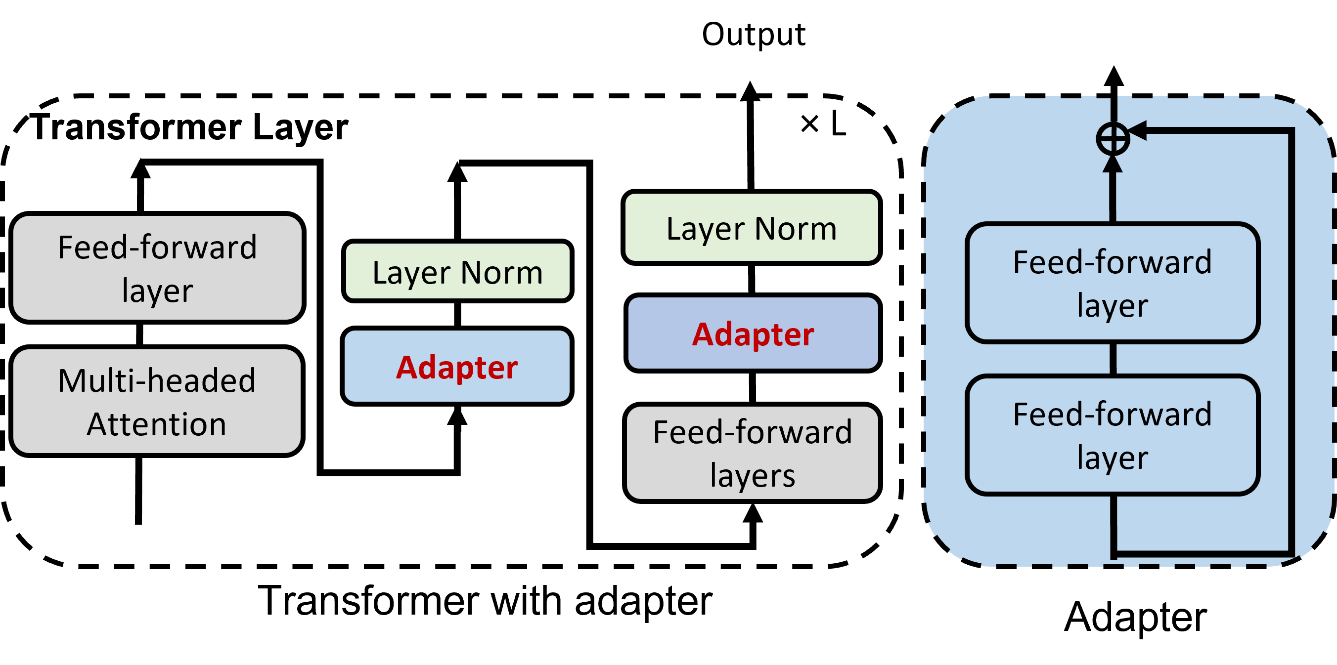
Figure 2: Architecture of Transformer with adapters. An adapter (blue component) is inserted in each layer. Only the blue and green boxes are trainable while the LM is fixed during training.

Appendix B Additional Details about the Datasets

Recall that TSS uses five datasets. Here we give their detailed statistics.

(1) ASC. ASC is more than the traditional sentiment classification because of the additional input of the aspect and the fact that in the same sentence different aspects can have different opinions. For example, “The picture is good but the sound is poor” about a TV expresses a positive opinion about the aspect “picture” and a negative opinion about the aspect “sound”. We show more details about these datasets in Table 3.

(2) CCD, SUM, DRG and NER. We give their detailed statistics in Table 4.

Tasks/Domains	#Training	#Validating	#Testing
Speaker	233 S./352 A./287 P./65 N./0 Ne.	30 S./44 A./35 P./9 N./0 Ne.	38 S./44 A./40 P./4 N./0 Ne.
Router	200 S./245 A./142 P./103 N./0 Ne.	24 S./31 A./19 P./12 N./0 Ne.	22 S./31 A./24 P./7 N./0 Ne.
Computer	187 S./283 A./218 P./65 N./0 Ne.	25 S./35 A./23 P./12 N./0 Ne.	29 S./36 A./29 P./7 N./0 Ne.
Nokia6610	209 S./271 A./198 P./73 N./0 Ne.	29 S./34 A./30 P./4 N./0 Ne.	28 S./34 A./25 P./9 N./0 Ne.
Nikon4300	131 S./162 A./135 P./27 N./0 Ne.	15 S./20 A./18 P./2 N./0 Ne.	15 S./21 A./19 P./2 N./0 Ne.
Creative	582 S./677 A./422 P./255 N./0 Ne.	68 S./85 A./42 P./43 N./0 Ne.	70 S./85 A./52 P./33 N./0 Ne.
CanonG3	190 S./228 A./180 P./48 N./0 Ne.	25 S./29 A./21 P./8 N./0 Ne.	24 S./29 A./24 P./5 N./0 Ne.
ApexAD	281 S./343 A./146 P./197 N./0 Ne.	35 S./43 A./16 P./27 N./0 Ne.	28 S./43 A./31 P./12 N./0 Ne.
CanonD500	103 S./118 A./96 P./22 N./0 Ne.	11 S./15 A./14 P./1 N./0 Ne.	13 S./15 A./11 P./4 N./0 Ne.
Canon100	137 S./175 A./123 P./52 N./0 Ne.	19 S./22 A./20 P./2 N./0 Ne.	16 S./22 A./21 P./1 N./0 Ne.
Diaper	166 S./191 A./143 P./48 N./0 Ne.	22 S./24 A./18 P./6 N./0 Ne.	24 S./24 A./22 P./2 N./0 Ne.
Hitachi	152 S./212 A./153 P./59 N./0 Ne.	23 S./26 A./19 P./7 N./0 Ne.	23 S./27 A./14 P./13 N./0 Ne.
Ipod	124 S./153 A./101 P./52 N./0 Ne.	18 S./19 A./14 P./5 N./0 Ne.	19 S./20 A./15 P./5 N./0 Ne.
Linksys	152 S./176 A./128 P./48 N./0 Ne.	19 S./22 A./13 P./9 N./0 Ne.	20 S./23 A./16 P./7 N./0 Ne.
MicroMP3	384 S./484 A./340 P./144 N./0 Ne.	42 S./61 A./48 P./13 N./0 Ne.	51 S./61 A./39 P./22 N./0 Ne.
Nokia6600	298 S./362 A./244 P./118 N./0 Ne.	26 S./45 A./32 P./13 N./0 Ne.	39 S./46 A./30 P./16 N./0 Ne.
Norton	168 S./194 A./54 P./140 N./0 Ne.	17 S./24 A./15 P./9 N./0 Ne.	24 S./25 A./5 P./20 N./0 Ne.
Restaurant	1893 S./3452 A./2094 P./779 N./579 Ne.	84 S./150 A./70 P./26 N./54 Ne.	600 S./1120 A./728 P./196 N./196 Ne.
Laptop	1360 S./2163 A./930 P./800 N./433 Ne.	98 S./150 A./57 P./66 N./27 Ne.	411 S./638 A./341 P./128 N./169 Ne.

Table 3: Statistics of the ASC tasks. S.: number of sentences; A: number of aspects; P., N., and Ne.: number aspects with positive, negative and neutral opinions, respectively. Note that the “Restaurant” and “Laptop” have 3 classes of opinion polarities (positive, negative and neutral) while the others have only 2 classes (positive and negative).

Dataset	Tasks/Domains	#Training	#Validating	#Testing	#Classes
CCD	Yahoo	4500	500	4840	10
	AGnews	1785	199	1756	2
	Amazon	898	100	998	2
	Dbpedia	6237	693	6748	14
	Yelp	900	100	984	4
SUM	icsi	43	10	6	—
	ami	97	20	20	—
	reddit	201	50	250	—
	stack	205	50	250	—
	nyt	200	50	250	—
	emails	215	50	250	—
DRG	taxi	406	71	56	—
	hotel	3366	143	177	—
	attraction	298	27	28	—
	train	1954	196	262	—
	restaurant	569	63	59	—
NER	conll2003	200	3250	3453	9
	wikigold	200	170	170	9
	btc	200	934	934	9
	re3d	200	77	200	21
	gum	200	250	1000	23

Table 4: Statistics of the CCD, SUM, DRE and NER datasets. Number of classes is not applicable to SUM and DRG because they are generation datasets.

Appendix C Hyperparameters

Unless otherwise stated, the same hyper-parameters are used in all experiments. The maximum input length is set to 128 for all datasets except for SUM which uses 1024 due to its longer sequences. AdamW optimizer is used. The learning rate is set to 5e-5 for Transformer (search within {5e-2,5e-3,5e-4,5e-5}), 3e-2 for prompt (search within {3e-1,3e-2,3e-3,3e-4,3e-5}), adapter and classifier. The prompt length is set to 20 (search within {10,20,50,80,100,150}) and adapter bottleneck size is 64, following the original paper (Houlsby et al., 2019). The batch size is set to 32 and the number of training epochs is set to 50 with early stopping. $\tau$ in Eq. 1 is set to 0. For classification tasks, a separate classification head is used for each task in the sequence. For generation tasks, a shared LM head is used for all tasks in a sequence. we further set the number of beams to 4 for beam search and constrain the target length in between 30 to 200. For image-based (EWC, Cuber, DAS, HAT, SupSup, CAT, L2P) and RoBERTa-based (CTR) systems, we adapt them for text classification and generation by replacing their feature extractors with BART. For LAMOL, we directly run the author provided code. Except for the aforementioned hyper-parameters, all baseline-specific hyper-parameters follow those in their original papers.

Appendix D Details of CL Baselines

5 adapter-based methods (CTR (Ke et al., 2021a), HAT (Serrà et al., 2018), SupSup (Wortsman et al., 2020), CAT (Ke et al., 2020) and CUBER (Lin et al., 2022a)). They all train a shared adapter while SupSup trains popup scores to indicate sub-network on the fixed adapter. HAT is one of the most effective TIL methods with little forgetting. CTR encourages transfer via capsule networks and transfer routing. SupSup uses the similar sub-network discovery method as TSS but cannot do KT at all. CAT and CTR are two systems that deal with both CF and KT. CUBER also deals with CF and KT, but a hard threshold is needed.

1 prompt-based method (L2P (Wang et al., 2022)), which trains a prompt pool to transfer task knowledge and a key-value pair prompt selection strategy to select the task-specific prompt (it thus deals with both KT and CF).

3 baselines that modify the Transformer (LAMOL (Sun et al., 2020), EWC (Kirkpatrick et al., 2016) and DAS Ke et al. (2023)). LAMOL is a pseudo-replay method using GPT-2. EWC is a regularization method. DAS is a soft-masking method aims to achieve both forgetting prevention and knowledge transfer for continual pre-training. Unlike TSS, it does not discover any sub-network and thus still suffers from forgetting.

Appendix E Detailed Results for Each System

In Tables 1 and  2 in the main paper, we only report the results of the main metrics (MF1 in ASC and CCD, F1 in NER, R1 in SUM and BLEU in DRG). In this section, we give all the results of all the other metrics. We report the detailed results in Tables 5 and 6, we can see TSS is effective in all other metrics.

	Similar			Dissimilar						Average	Average
Dataset	ASC		NER	SUM			CCD		DRG
Model	MF1	Acc	F1	R1	R2	RL	MF1	Acc	BLEU	Main	FR
Non-continual learning
MTL	92.28	94.82	63.33	39.39	10.33	35.05	90.57	90.55	25.29	62.17	—
MTL (Adapter)	92.17	94.65	60.61	38.84	11.38	34.81	91.09	91.14	24.50	61.44	—
ONE	85.55	91.50	59.33	39.07	10.71	35.25	91.07	91.09	24.14	59.83	—
ONE (Adapter)	83.95	90.90	56.69	38.90	11.54	35.23	90.78	90.81	23.42	58.75	—
ONE (Prompt)	76.46	85.54	45.90	30.67	7.23	27.53	86.23	86.28	12.67	50.39	—
Continual learning of heterogeneous Tasks
NCL	88.05	92.60	34.56	22.86	4.67	20.61	81.86	82.70	8.68	47.20	13.94
EWC	88.73	92.86	28.75	18.65	21.22	16.36	83.24	83.92	7.99	45.47	13.43
HAT	87.45	92.77	50.16	35.21	9.96	31.83	89.85	90.03	20.98	56.73	0.97
DAS	90.62	93.73	43.38	25.45	5.88	23.08	82.66	84.39	15.21	51.47	10.49
SupSup	85.83	92.41	58.93	38.23	11.44	34.88	90.66	90.68	24.71	59.67	0.00
CAT	45.79	50.08	35.24	17.44	2.43	15.50	36.62	39.01	10.21	29.06	30.27
CTR	89.37	93.28	50.16	33.98	9.97	30.80	89.96	89.98	17.63	56.22	0.95
CUBER	90.58	93.72	46.67	30.94	7.30	27.92	81.54	81.41	15.68	53.08	7.52
L2P	78.10	87.97	39.03	28.34	5.93	25.44	72.35	76.99	4.55	44.47	6.44
TSS	90.61	94.47	62.13	38.29	11.77	35.26	90.70	90.70	24.56	61.26	0.00
Continual learning of homogeneous Tasks
CL	89.25	93.04	49.19	32.68	6.84	29.19	85.08	85.10	22.31	55.70	6.42
EWC	88.36	92.60	51.76	32.64	7.12	29.00	87.27	87.37	18.30	55.66	5.53
HAT	89.33	93.28	52.31	37.11	10.40	33.53	90.21	90.23	21.47	58.08	0.49
DAS	90.94	94.20	42.12	31.31	7.61	28.79	87.97	88.12	22.25	54.92	9.26
SupSup	85.83	92.41	58.93	38.23	11.44	34.88	90.66	90.68	24.71	59.67	0.00
LAMOL	84.62	90.17	—	10.88	1.39	6.87	54.44	67.04	19.96	—	—
CAT	84.31	88.98	50.73	37.24	10.53	33.77	90.82	90.90	21.72	56.96	1.37
CTR	88.86	92.94	51.85	37.34	10.73	33.69	90.54	90.58	21.39	58.00	0.65
CUBER	91.25	94.33	47.19	30.44	6.75	27.51	89.19	89.27	21.66	55.95	5.82
L2P	74.81	84.64	44.22	26.65	4.82	23.90	85.35	85.54	8.52	47.91	2.58
TSS	91.28	94.06	63.96	38.39	11.60	35.22	90.89	90.92	24.75	61.85	0.00

Table 5: Performance for heterogeneous (40 tasks in total) and homogeneous tasks, averaged over 5 random sequences (the standard deviation is reported in Table 9). “—” means not applicable. We bold the best performance within CL baselines.

	Similar			Dissimilar						Average	Average
Dataset	ASC		NER	SUM			CCD		DRG
Model	MF1	Acc	F1	R1	R2	RL	MF1	Acc	BLEU	Main	FR
Non-continual learning
ONE	85.55	91.50	59.33	39.07	10.71	35.25	91.07	91.09	24.14	59.83	—
Continual learning of heterogeneous Tasks
TSS (w/o SD)	86.54	71.55	37.03	28.04	6.39	25.57	78.29	61.91	14.85	48.95	9.02
TSS (w/o SM)	85.83	92.41	58.93	38.23	11.44	34.88	90.66	90.68	24.71	59.67	0.00
TSS (w/o SM; Naive)	88.89	93.36	34.79	36.11	10.27	33.15	89.99	89.99	24.19	54.80	0.00
TSS	90.61	94.47	62.13	38.29	11.77	35.26	90.70	90.70	24.56	61.26	0.00
Continual learning of homogeneous Tasks
TSS (w/o SD)	91.06	94.24	40.47	30.42	7.30	27.83	88.34	88.40	22.77	54.61	9.61
TSS (w/o SM)	85.83	92.41	58.93	38.23	11.44	34.88	90.66	90.68	24.71	59.67	0.00
TSS (w/o SM; Naive)	90.38	94.25	62.42	38.08	11.52	35.05	90.63	90.74	24.59	61.22	0.00
TSS	91.28	94.06	63.96	38.39	11.60	35.22	90.89	90.92	24.75	61.85	0.00

Table 6: Ablation experiment results for heterogeneous and homogeneous tasks - averages over 5 random sequences (the standard deviation is reported in Table 10).

	Similar			Dissimilar						Average
Dataset	ASC		NER	SUM			CCD		DRG
Model	MF1	Acc	F1	R1	R2	RL	MF1	Acc	BLEU	FR
Continual learning of heterogeneous Tasks
NCL	1.89	3.41	26.89	15.79	6.16	8.77	8.65	7.35	16.47	13.94
EWC	-0.16	0.57	29.29	19.50	6.70	10.33	3.06	6.53	15.46	13.43
HAT	-0.98	0.11	1.54	2.21	1.20	1.49	0.62	1.12	1.44	0.97
DAS	-0.44	0.01	21.66	13.48	5.65	7.32	8.02	7.86	9.73	10.49
SupSup	0.00	0.00	0.00	0.00	0.00	0.00	0.00	0.00	0.00	0.00
CAT	39.99	36.92	18.30	25.23	9.99	13.93	53.85	32.99	13.96	30.27
CTR	-0.15	-0.13	0.72	2.31	0.64	1.39	0.47	0.38	1.42	0.95
CUBER	-1.84	-1.72	12.98	11.54	5.09	6.65	1.56	1.55	12.09	7.27
L2P	2.53	0.09	4.04	5.84	2.87	3.99	12.66	11.31	7.16	6.44
TSS	0.00	0.00	0.00	0.00	0.00	0.00	0.00	0.00	0.00	0.00
Continual learning of homogeneous Tasks
NCL	-0.44	0.31	15.49	8.37	5.54	5.90	5.67	5.64	3.01	6.42
EWC	7.81	2.78	7.53	2.58	1.68	2.04	8.94	8.17	0.78	5.53
HAT	-0.88	-0.36	0.79	1.10	1.22	0.78	-0.07	-0.08	1.48	0.49
DAS	-0.81	-0.77	31.88	7.87	3.89	4.98	3.73	3.56	3.61	9.26
SupSup	0.00	0.00	0.00	0.00	0.00	0.00	0.00	0.00	0.00	0.00
LAMOL	-1.88	-1.52	—	3.90	1.42	2.32	32.26	27.30	2.29	—
CAT	2.05	0.81	0.81	1.85	1.41	1.37	-0.13	-0.21	2.26	1.37
CTR	-0.38	-0.08	0.58	1.43	0.90	0.86	-0.27	-0.27	1.91	0.65
CUBER	-0.38	-0.08	0.58	1.43	0.90	0.86	-0.27	-0.27	1.91	0.65
L2P	0.30	0.54	0.96	7.27	3.53	4.68	0.94	0.82	3.42	2.58
TSS	0.00	0.00	0.00	0.00	0.00	0.00	0.00	0.00	0.00	0.00

Table 7: Forgetting rate for heterogeneous (40 tasks in total) and homogeneous tasks, averaged over 5 random sequences.

Appendix F Difference between our forgetting rate and the one in (Mehta et al., 2021)

Unlike our forgetting rate in Sec. 4, the forgetting rate in (Mehta et al., 2021) is defined as $F^{\prime}_{t}=\frac{1}{t-1}\sum_{\tau=1}^{t-1}\text{max}_{\tau^{\prime}\in\{1,...,t-1\}}(S_{\tau^{\prime},\tau}-S_{t,\tau})$. Since both metrics measure everything from the standing point of the end of continual learning, i.e., after all tasks are learned, we believe our measure is more reasonable. Let us use some examples to illustrate,

• (1). if task 1 archives the accuracy 0.5 right after its training, it achieves 0.4 after task 2, and it achieves 0.3 after task 3 (final task). In this case, both measures give the same forgetting 0.2.

• (2). if task 1 archives the accuracy 0.5 right after its training, it achieves 0.8 after task 2, and it achieves 0.82 after task 3 (final task). If we take max ($F_{t}^{\prime}$), then the forgetting is -0.02, but our method will give -0.32. In this case, our method is more reasonable because it precisely shows how much backward transfer (negative value here means backward transfer) has been achieved for task 1 after task 2 and task 3 are learned since both measures evaluate from the same reference point, i.e., after all tasks are learned (the last task is t in both measures, i.e., task 3 in this example).

• (3). If task 1 archives the accuracy 0.5 right after its training, 0.8 after task 2 and 0.4 after task 3 (final task), our metric will give the forgetting 0.1. $F_{t}^{\prime}$ will give 0.4. This case is more debatable because $F_{t}^{\prime}$ catches the worst forgetting. But since we evaluate after all tasks are learned (the reference point is when the last task is learned), again we believe that our method is more reasonable.

• (4). If task 1 archives the accuracy 0.5 right after its training, 0.1 after task 2 and 0.4 after task 3 (final task), both metrics will give the forgetting 0.1. In this case, $F_{t}^{\prime}$ does not catch the worst forgetting of 0.4 (0.5-0.1) in the process. Again, if we agree that we evaluate from the reference point of when the last task is learned, then both measures are fine in this case.

In summary, while we believe ours is more reasonable, a better metric may be designed in the future to characterize forgetting and knowledge transfer in the continual learning process.

Appendix G Detailed Forgetting Rate for Each Dataset

We report the average forgetting rate of each system in Tables 1 and 2 (in the main paper). In this section, we report the detailed forgetting rate of each system corresponding to each of the above tables.

Table 7 and Table 8 show the detailed forgetting rate for both heterogeneous and homogeneous tasks.

In heterogeneous tasks, we can see on average TSS and SupSup have the lowest forgetting rate (TSS outperforms SupSup in final performances due to knowledge transfer). While some baselines (e.g. DAS, CUBER, EWC) have a negative forgetting rate (indicating the new knowledge helps similar old tasks), they suffer from large forgetting in dissimilar tasks because they cannot do well in forgetting.

In homogeneous tasks, similar to the heterogeneous tasks, we can see on average TSS and SupSup have the lowest forgetting rate (TSS outperforms SupSup in final performances due to knowledge transfer). We also notice the forgetting is in general less than heterogeneous tasks because the tasks in heterogeneous sequence can be more dissimilar (e.g., from summarization to NER).

	Similar			Dissimilar						Average
Dataset	ASC		NER	SUM			CCD		DRG
Model	MF1	Acc	F1	R1	R2	RL	MF1	Acc	BLEU	FR
Continual learning of heterogeneous Tasks
TSS (w/o SD)	-0.48	0.24	20.90	8.88	4.19	4.57	8.38	8.53	7.41	9.02
TSS (w/o SM)	0.00	0.00	0.00	0.00	0.00	0.00	0.00	0.00	0.00	0.00
TSS (w/o SM; Naive)	0.00	0.00	0.00	0.00	0.00	0.00	0.00	0.00	0.00	0.00
TSS	0.00	0.00	0.00	0.00	0.00	0.00	0.00	0.00	0.00	0.00
Continual learning of homogeneous Tasks
TSS (w/o SD)	-1.71	-0.77	34.14	10.18	4.94	6.62	2.83	2.74	2.62	9.61
TSS (w/o SM)	0.00	0.00	0.00	0.00	0.00	0.00	0.00	0.00	0.00	0.00
TSS (w/o SM; Naive)	0.00	0.00	0.00	0.00	0.00	0.00	0.00	0.00	0.00	0.00
TSS	0.00	0.00	0.00	0.00	0.00	0.00	0.00	0.00	0.00	0.00

Table 8: Forgetting rate for ablation of heterogeneous tasks (40 tasks in total) and homogeneous tasks, averaged over 5 random sequences.

	Similar			Dissimilar
Dataset	ASC		NER	SUM			CCD		DRG
Model	MF1	Acc	F1	R1	R2	RL	MF1	Acc	BLEU
Continual learning of heterogeneous tasks
NCL	$\pm$0.0133	$\pm$0.0043	$\pm$0.1397	$\pm$0.1079	$\pm$0.0251	$\pm$0.0954	$\pm$0.0150	$\pm$0.0044	$\pm$0.0527
EWC	$\pm$0.0114	$\pm$0.0050	$\pm$0.1278	$\pm$0.1047	$\pm$0.2167	$\pm$0.0947	$\pm$0.0171	$\pm$0.0155	$\pm$0.0914
HAT	$\pm$0.0395	$\pm$0.0152	$\pm$0.0078	$\pm$0.0041	$\pm$0.0024	$\pm$0.0046	$\pm$0.0020	$\pm$0.0023	$\pm$0.0119
DAS	$\pm$0.0126	$\pm$0.0072	$\pm$0.0348	$\pm$0.1116	$\pm$0.0300	$\pm$0.1000	$\pm$0.0241	$\pm$0.0375	$\pm$0.0638
CAT	$\pm$0.1732	$\pm$0.2137	$\pm$0.0034	$\pm$0.0549	$\pm$0.0318	$\pm$0.0794	$\pm$0.1176	$\pm$0.2163	$\pm$0.0333
CTR	$\pm$0.0447	$\pm$0.0023	$\pm$0.0712	$\pm$0.0278	$\pm$0.0058	$\pm$0.0029	$\pm$0.1492	$\pm$0.0385	$\pm$0.0704
CUBER	$\pm$0.0175	$\pm$0.0107	$\pm$0.0589	$\pm$0.0682	$\pm$0.0208	$\pm$0.0598	$\pm$0.0394	$\pm$0.0396	$\pm$0.0631
L2P	$\pm$0.0173	$\pm$0.0260	$\pm$0.0225	$\pm$0.0328	$\pm$0.0153	$\pm$0.0298	$\pm$0.0759	$\pm$0.0494	$\pm$0.0287
TSS	$\pm$0.0058	$\pm$0.0124	$\pm$0.0503	$\pm$0.0025	$\pm$0.0018	$\pm$0.0021	$\pm$0.0047	$\pm$0.0034	$\pm$0.0058
Continual learning of homogeneous tasks
NCL	$\pm$0.0040	$\pm$0.0027	$\pm$0.0767	$\pm$0.0060	$\pm$0.0055	$\pm$0.0066	$\pm$0.0233	$\pm$0.0230	$\pm$0.0060
EWC	$\pm$0.0093	$\pm$0.0063	$\pm$0.0707	$\pm$0.0132	$\pm$0.0053	$\pm$0.0113	$\pm$0.0227	$\pm$0.0216	$\pm$0.0217
HAT	$\pm$0.0130	$\pm$0.0042	$\pm$0.0063	$\pm$0.0130	$\pm$0.0049	$\pm$0.0115	$\pm$0.0028	$\pm$0.0028	$\pm$0.0094
DAS	$\pm$0.0075	$\pm$0.0024	$\pm$0.0647	$\pm$0.0091	$\pm$0.0070	$\pm$0.0074	$\pm$0.0178	$\pm$0.0175	$\pm$0.0094
LAMOL	$\pm$0.0085	$\pm$0.0039	—	$\pm$0.0125	$\pm$0.0042	$\pm$0.0052	$\pm$0.0317	$\pm$0.0258	$\pm$0.0068
CAT	$\pm$0.0096	$\pm$0.0021	$\pm$0.0106	$\pm$0.0104	$\pm$0.0040	$\pm$0.0090	$\pm$0.0019	$\pm$0.0021	$\pm$0.0051
CTR	$\pm$0.0080	$\pm$0.0030	$\pm$0.0049	$\pm$0.0116	$\pm$0.0052	$\pm$0.0096	$\pm$0.0009	$\pm$0.0010	$\pm$0.0127
CUBER	$\pm$0.0072	$\pm$0.0031	$\pm$0.0543	$\pm$0.0157	$\pm$0.0061	$\pm$0.0119	$\pm$0.0069	$\pm$0.0062	$\pm$0.0090
L2P	$\pm$0.0650	$\pm$0.0361	$\pm$0.0022	$\pm$0.0215	$\pm$0.0047	$\pm$0.0203	$\pm$0.0181	$\pm$0.0176	$\pm$0.0216
TSS	$\pm$0.0031	$\pm$0.0035	$\pm$0.0032	$\pm$0.0021	$\pm$0.0020	$\pm$0.0015	$\pm$0.0024	$\pm$0.0026	$\pm$0.0035

Table 9: Standard deviations of the corresponding metrics of the proposed TSS model and the baselines on the heterogeneous and homogeneous tasks.

	Similar			Dissimilar
Dataset	ASC		NER	SUM			CCD		DRG
Model	MF1	Acc	F1	R1	R2	RL	MF1	Acc	BLEU
Continual learning of heterogeneous tasks
TSS (w/o SD)	$\pm$0.0866	$\pm$0.3657	$\pm$0.1328	$\pm$0.0536	$\pm$0.0216	$\pm$0.0473	$\pm$0.0942	$\pm$0.3222	$\pm$0.0541
TSS (w/o SM; Naive)	$\pm$0.0096	$\pm$0.0063	$\pm$0.0307	$\pm$0.0106	$\pm$0.0063	$\pm$0.0107	$\pm$0.0028	$\pm$0.0029	$\pm$0.0049
TSS	$\pm$0.0058	$\pm$0.0124	$\pm$0.0503	$\pm$0.0025	$\pm$0.0018	$\pm$0.0021	$\pm$0.0047	$\pm$0.0034	$\pm$0.0058
Continual learning of homogeneous tasks
TSS (w/o SD)	$\pm$0.0107	$\pm$0.0066	$\pm$0.0695	$\pm$0.0088	$\pm$0.0056	$\pm$0.0071	$\pm$0.0274	$\pm$0.0268	$\pm$0.0039
TSS (w/o SM; Naive)	$\pm$0.0102	$\pm$0.0040	$\pm$0.0067	$\pm$0.0024	$\pm$0.0014	$\pm$0.0023	$\pm$0.0019	$\pm$0.0016	$\pm$0.0019
TSS	$\pm$0.0031	$\pm$0.0035	$\pm$0.0032	$\pm$0.0021	$\pm$0.0020	$\pm$0.0015	$\pm$0.0024	$\pm$0.0026	$\pm$0.0035

Table 10: Standard deviations of the corresponding metrics of the proposed TSS model and the ablation experiments on the heterogeneous and homogeneous tasks.

Appendix H Standard Deviations

This section reports the standard deviations of the corresponding results in Tables 1 and 2 (in the main paper) of TSS and the considered baselines over 5 runs with random sequences. We only report the CL baselines since they are related to the task order. We can see the results of TSS is stable. SupSup and TSS (w/o SM) discover different sub-networks for different tasks, so they are not related to the task order and are not reported in the table. We report the standard deviations for all metrics for completeness.

In heterogeneous tasks, Table 9 and Table 10 report the standard deviations of TSS and the considered baselines over 5 runs with random sequences. We can see the results of TSS and its variants are stable.

In homogeneous tasks, similar to heterogeneous tasks, we can see the results of TSS and its variants are stable.

Task	Order	Similar			Dissimilar						Average
		ASC		NER	SUM			CCD		DRG
		MF1	Acc	F1	R1	R2	RL	MF1	Acc	BLEU	Main
Heterogeneous	0	90.61	94.47	62.13	38.29	11.77	35.26	90.70	90.70	24.56	61.26
	1	90.07	93.66	62.00	38.56	11.65	35.35	90.21	90.23	24.25	61.02
	2	89.34	93.46	48.83	37.80	11.33	34.75	91.35	91.20	25.92	58.65
	3	89.59	93.65	58.53	38.39	11.78	35.24	90.24	90.81	25.25	60.40
	4	88.95	90.82	61.25	38.31	11.45	35.09	90.07	90.38	25.07	60.73
Homogeneous	0	91.57	94.40	63.96	38.46	11.38	35.19	91.02	91.08	24.89	61.98
	1	91.65	94.45	63.19	38.53	11.62	35.28	90.84	90.86	24.07	61.66
	2	90.96	93.62	63.26	38.58	11.85	35.40	91.28	91.34	24.81	61.78
	3	91.48	94.39	63.01	38.14	11.72	35.06	90.65	90.65	25.02	61.66
	4	90.94	93.78	63.37	38.06	11.33	34.97	90.65	90.67	24.97	61.60

Table 11: Results for TSS in different orders for heterogeneous and homogeneous tasks.

Appendix I Results for Individual Sequences

In Table 1 in the main text, we reported the results averaged over 5 random sequences (different task orders). In this section, we give the results of TSS of each sequence in Table 11. We can see that the order indeed affects the results but not by much. In summary, we believe the average over random sequences in Table 1 (in the main text/paper) can show the effectiveness of TSS.

Appendix J Execution Time and Number of Parameters

Table 12 reports the number of parameters (regardless of trainable or non-trainable), training execution times for different CL models. Our experiments were run on 4 GeForce GTX 2080 Ti with 48G GPUs memory. We only report the training time for heterogenous tasks because the training time is related to datasets and one of the main goal of TSS is to work well in the challenging heterogeneous scenario. we can see TSS is very efficient, ranking among the least number of parameters and shortest training time among all the baselines considered.

Saved binary gates for each task. For each task, the memory usage for the saved binary gates is on average 3.1M bytes, which is 7 times less than saving all the information of the adapter (25.2M), not to mention if one saves the whole LM (3.6G). The number of accumulated importance values is constant, which has the same size as the adapter.

Model	#Params (M)	Training time (min)
NCL	896.9	600
EWC	896.9	600
HAT	958.0	600
DAS	896.9	600
LAMOL	124.4	550
CAT	896.9	24,000
CTR	1,536	48,000
CUBER	896.9	600
L2P	899.0	650
TSS	896.9	600

Table 12: Network size (#parameters in millions, regardless of trainable or non-trainable) and average training time per task of each CL model measured in minutes for heterogenous tasks. Here we report #parameters without including the memory buffer.

References

- Balasuriya et al. (2009) Dominic Balasuriya, Nicky Ringland, Joel Nothman, Tara Murphy, and James R. Curran. 2009. Named entity recognition in wikipedia. In Proceedings of the 1st 2009 Workshop on The People’s Web Meets NLP: Collaboratively Constructed Semantic Resources@IJCNLP 2009, Suntec, Singapore, August 7, 2009, pages 10–18. Association for Computational Linguistics.
- Bengio et al. (2013) Yoshua Bengio, Nicholas Léonard, and Aaron C. Courville. 2013. Estimating or propagating gradients through stochastic neurons for conditional computation. CoRR, abs/1308.3432.
- Chaudhry et al. (2019) Arslan Chaudhry, Marc’Aurelio Ranzato, Marcus Rohrbach, and Mohamed Elhoseiny. 2019. Efficient lifelong learning with A-GEM. In ICLR.
- Chen et al. (2020) Tianlong Chen, Jonathan Frankle, Shiyu Chang, Sijia Liu, Yang Zhang, Zhangyang Wang, and Michael Carbin. 2020. The lottery ticket hypothesis for pre-trained bert networks. Advances in neural information processing systems, 33:15834–15846.
- Chen and Liu (2018) Zhiyuan Chen and Bing Liu. 2018. Lifelong machine learning. Synthesis Lectures on Artificial Intelligence and Machine Learning, 12(3):1–207.
- de Masson d’Autume et al. (2019) Cyprien de Masson d’Autume, Sebastian Ruder, Lingpeng Kong, and Dani Yogatama. 2019. Episodic memory in lifelong language learning. In Advances in Neural Information Processing Systems 32: Annual Conference on Neural Information Processing Systems 2019, NeurIPS 2019, December 8-14, 2019, Vancouver, BC, Canada.
- Derczynski et al. (2016) Leon Derczynski, Kalina Bontcheva, and Ian Roberts. 2016. Broad twitter corpus: A diverse named entity recognition resource. In COLING 2016, 26th International Conference on Computational Linguistics, Proceedings of the Conference: Technical Papers, December 11-16, 2016, Osaka, Japan, pages 1169–1179. ACL.
- Fabbri et al. (2021) Alexander R. Fabbri, Faiaz Rahman, Imad Rizvi, Borui Wang, Haoran Li, Yashar Mehdad, and Dragomir R. Radev. 2021. Convosumm: Conversation summarization benchmark and improved abstractive summarization with argument mining. In Proceedings of the 59th Annual Meeting of the Association for Computational Linguistics and the 11th International Joint Conference on Natural Language Processing, ACL/IJCNLP 2021, (Volume 1: Long Papers), Virtual Event, August 1-6, 2021, pages 6866–6880. Association for Computational Linguistics.
- Fan et al. (2020) Angela Fan, Edouard Grave, and Armand Joulin. 2020. Reducing transformer depth on demand with structured dropout. In International Conference on Learning Representations.
- Fernando et al. (2017) Chrisantha Fernando, Dylan Banarse, Charles Blundell, Yori Zwols, David Ha, Andrei A. Rusu, Alexander Pritzel, and Daan Wierstra. 2017. Pathnet: Evolution channels gradient descent in super neural networks. CoRR.
- Gao et al. (2021) Yang Gao, Nicolo Colombo, and Wei Wang. 2021. Adapting by pruning: A case study on bert. arXiv preprint arXiv:2105.03343.
- He and Jaeger (2018) Xu He and Herbert Jaeger. 2018. Overcoming catastrophic interference using conceptor-aided backpropagation. In ICLR.
- Houlsby et al. (2019) Neil Houlsby, Andrei Giurgiu, Stanislaw Jastrzebski, Bruna Morrone, Quentin de Laroussilhe, Andrea Gesmundo, Mona Attariyan, and Sylvain Gelly. 2019. Parameter-efficient transfer learning for NLP. In ICML.
- Huang et al. (2021) Yufan Huang, Yanzhe Zhang, Jiaao Chen, Xuezhi Wang, and Diyi Yang. 2021. Continual learning for text classification with information disentanglement based regularization. arXiv preprint arXiv:2104.05489.
- Kamra et al. (2017) Nitin Kamra, Umang Gupta, and Yan Liu. 2017. Deep generative dual memory network for continual learning. CoRR.
- Ke and Liu (2022) Zixuan Ke and Bing Liu. 2022. Continual learning of natural language processing tasks: A survey. arXiv preprint arXiv:2211.12701.
- Ke et al. (2020) Zixuan Ke, Bing Liu, and Xingchang Huang. 2020. Continual learning of a mixed sequence of similar and dissimilar tasks. In NeurIPS.
- Ke et al. (2021a) Zixuan Ke, Bing Liu, Nianzu Ma, Hu Xu, and Lei Shu. 2021a. Achieving forgetting prevention and knowledge transfer in continual learning. Advances in Neural Information Processing Systems, 34.
- Ke et al. (2023) Zixuan Ke, Yijia Shao, Haowei Lin, Tatsuya Konishi, Gyuhak Kim, and Bing Liu. 2023. Continual pre-training of language models. In The Eleventh International Conference on Learning Representations.
- Ke et al. (2021b) Zixuan Ke, Hu Xu, and Bing Liu. 2021b. Adapting bert for continual learning of a sequence of aspect sentiment classification tasks. In NAACL.
- Kim et al. (2022) Gyuhak Kim, Changnan Xiao, Tatsuya Konishi, Zixuan Ke, and Bing Liu. 2022. A theoretical study on solving continual learning. In Advances in Neural Information Processing Systems.
- Kim et al. (2023) Gyuhak Kim, Changnan Xiao, Tatsuya Konishi, and Bing Liu. 2023. Learnability and algorithm for continual learning. arXiv preprint arXiv:2306.12646.
- Kirkpatrick et al. (2016) James Kirkpatrick, Razvan Pascanu, Neil C. Rabinowitz, Joel Veness, Guillaume Desjardins, Andrei A. Rusu, Kieran Milan, John Quan, Tiago Ramalho, Agnieszka Grabska-Barwinska, Demis Hassabis, Claudia Clopath, Dharshan Kumaran, and Raia Hadsell. 2016. Overcoming catastrophic forgetting in neural networks. CoRR.
- Konishi et al. (2023) Tatsuya Konishi, Mori Kurokawa, Chihiro Ono, Zixuan Ke, Gyuhak Kim, and Bing Liu. 2023. Parameter-level soft-masking for continual learning. Proceedingsofthe40thInternationalConferenceonMachine Learning (ICML-2023).
- Laboratory (2017) Defence Science Technology Laboratory. 2017. Relationship and entity extraction evaluation dataset.
- Lai et al. (2021) Cheng-I Jeff Lai, Yang Zhang, Alexander H Liu, Shiyu Chang, Yi-Lun Liao, Yung-Sung Chuang, Kaizhi Qian, Sameer Khurana, David Cox, and Jim Glass. 2021. Parp: Prune, adjust and re-prune for self-supervised speech recognition. NeurIPS, 34.
- Lee et al. (2017) Sang-Woo Lee, Jin-Hwa Kim, Jaehyun Jun, Jung-Woo Ha, and Byoung-Tak Zhang. 2017. Overcoming catastrophic forgetting by incremental moment matching. In NIPS.
- Lewis et al. (2020) Mike Lewis, Yinhan Liu, Naman Goyal, Marjan Ghazvininejad, Abdelrahman Mohamed, Omer Levy, Veselin Stoyanov, and Luke Zettlemoyer. 2020. BART: denoising sequence-to-sequence pre-training for natural language generation, translation, and comprehension. In Proceedings of the 58th Annual Meeting of the Association for Computational Linguistics, ACL 2020, Online, July 5-10, 2020, pages 7871–7880. Association for Computational Linguistics.
- Li et al. (2021) Jiaoda Li, Ryan Cotterell, and Mrinmaya Sachan. 2021. Differentiable subset pruning of transformer heads. Transactions of the Association for Computational Linguistics, 9:1442–1459.
- Lin et al. (2022a) Sen Lin, Li Yang, Deliang Fan, and Junshan Zhang. 2022a. Beyond not-forgetting: Continual learning with backward knowledge transfer. NeurIPS.
- Lin et al. (2022b) Sen Lin, Li Yang, Deliang Fan, and Junshan Zhang. 2022b. Trgp: Trust region gradient projection for continual learning. arXiv preprint arXiv:2202.02931.
- Lin et al. (2020) Zi Lin, Jeremiah Zhe Liu, Zi Yang, Nan Hua, and Dan Roth. 2020. Pruning redundant mappings in transformer models via spectral-normalized identity prior. arXiv preprint arXiv:2010.01791.
- Liu et al. (2020) Yaoyao Liu, Yuting Su, An-An Liu, Bernt Schiele, and Qianru Sun. 2020. Mnemonics training: Multi-class incremental learning without forgetting. In CVPR.
- Lopez-Paz and Ranzato (2017) David Lopez-Paz and Marc’Aurelio Ranzato. 2017. Gradient episodic memory for continual learning. In NIPS.
- Madotto et al. (2020) Andrea Madotto, Zhaojiang Lin, Zhenpeng Zhou, Seungwhan Moon, Paul Crook, Bing Liu, Zhou Yu, Eunjoon Cho, and Zhiguang Wang. 2020. Continual learning in task-oriented dialogue systems. arXiv preprint arXiv:2012.15504.
- Mallya and Lazebnik (2018) Arun Mallya and Svetlana Lazebnik. 2018. Packnet: Adding multiple tasks to a single network by iterative pruning. In CVPR.
- McCarley et al. (2019) JS McCarley, Rishav Chakravarti, and Avirup Sil. 2019. Structured pruning of a bert-based question answering model. arXiv preprint arXiv:1910.06360.
- Mehta et al. (2021) Sanket Vaibhav Mehta, Darshan Patil, Sarath Chandar, and Emma Strubell. 2021. An empirical investigation of the role of pre-training in lifelong learning. CoRR, abs/2112.09153.
- Michel et al. (2019) Paul Michel, Omer Levy, and Graham Neubig. 2019. Are sixteen heads really better than one? Advances in neural information processing systems, 32.
- Qin and Joty (2022) Chengwei Qin and Shafiq R. Joty. 2022. LFPT5: A unified framework for lifelong few-shot language learning based on prompt tuning of T5. In The Tenth International Conference on Learning Representations, ICLR 2022, Virtual Event, April 25-29, 2022. OpenReview.net.
- Ramadan et al. (2018) Osman Ramadan, Paweł Budzianowski, and Milica Gasic. 2018. Large-scale multi-domain belief tracking with knowledge sharing. In Proceedings of the 56th Annual Meeting of the Association for Computational Linguistics, volume 2, pages 432–437.
- Ramanujan et al. (2020) Vivek Ramanujan, Mitchell Wortsman, Aniruddha Kembhavi, Ali Farhadi, and Mohammad Rastegari. 2020. What’s hidden in a randomly weighted neural network? In 2020 IEEE/CVF Conference on Computer Vision and Pattern Recognition, CVPR 2020, Seattle, WA, USA, June 13-19, 2020, pages 11890–11899. Computer Vision Foundation / IEEE.
- Rebuffi et al. (2017) Sylvestre-Alvise Rebuffi, Alexander Kolesnikov, Georg Sperl, and Christoph H. Lampert. 2017. icarl: Incremental classifier and representation learning. In CVPR.
- Rostami et al. (2019) Mohammad Rostami, Soheil Kolouri, and Praveen K. Pilly. 2019. Complementary learning for overcoming catastrophic forgetting using experience replay. In IJCAI.
- Rusu et al. (2016) Andrei A. Rusu, Neil C. Rabinowitz, Guillaume Desjardins, Hubert Soyer, James Kirkpatrick, Koray Kavukcuoglu, Razvan Pascanu, and Raia Hadsell. 2016. Progressive neural networks. CoRR.
- Sajjad et al. (2020) Hassan Sajjad, Fahim Dalvi, Nadir Durrani, and Preslav Nakov. 2020. On the effect of dropping layers of pre-trained transformer models. arXiv preprint arXiv:2004.03844.
- Sang and Meulder (2003) Erik F. Tjong Kim Sang and Fien De Meulder. 2003. Introduction to the conll-2003 shared task: Language-independent named entity recognition. In Proceedings of the Seventh Conference on Natural Language Learning, CoNLL 2003, Held in cooperation with HLT-NAACL 2003, Edmonton, Canada, May 31 - June 1, 2003, pages 142–147. ACL.
- Seff et al. (2017) Ari Seff, Alex Beatson, Daniel Suo, and Han Liu. 2017. Continual learning in generative adversarial nets. CoRR, abs/1705.08395.
- Serrà et al. (2018) Joan Serrà, Didac Suris, Marius Miron, and Alexandros Karatzoglou. 2018. Overcoming catastrophic forgetting with hard attention to the task. In ICML.
- Shin et al. (2017) Hanul Shin, Jung Kwon Lee, Jaehong Kim, and Jiwon Kim. 2017. Continual learning with deep generative replay. In NIPS.
- Sun et al. (2020) Fan-Keng Sun, Cheng-Hao Ho, and Hung-Yi Lee. 2020. Lamol: Language modeling is all you need for lifelong language learning. In ICLR.
- Voita et al. (2019) Elena Voita, David Talbot, Fedor Moiseev, Rico Sennrich, and Ivan Titov. 2019. Analyzing multi-head self-attention: Specialized heads do the heavy lifting, the rest can be pruned. arXiv preprint arXiv:1905.09418.
- Wang et al. (2021) Chengyu Wang, Haojie Pan, Yuan Liu, Kehan Chen, Minghui Qiu, Wei Zhou, Jun Huang, Haiqing Chen, Wei Lin, and Deng Cai. 2021. Mell: Large-scale extensible user intent classification for dialogue systems with meta lifelong learning. In KDD ’21: The 27th ACM SIGKDD Conference on Knowledge Discovery and Data Mining, Virtual Event, Singapore, August 14-18, 2021.
- Wang et al. (2022) Zifeng Wang, Zizhao Zhang, Chen-Yu Lee, Han Zhang, Ruoxi Sun, Xiaoqi Ren, Guolong Su, Vincent Perot, Jennifer Dy, and Tomas Pfister. 2022. Learning to prompt for continual learning. In CVPR.
- Wang et al. (2020) Zirui Wang, Sanket Vaibhav Mehta, Barnabás Póczos, and Jaime Carbonell. 2020. Efficient meta lifelong-learning with limited memory. In EMNLP.
- Wortsman et al. (2020) Mitchell Wortsman, Vivek Ramanujan, Rosanne Liu, Aniruddha Kembhavi, Mohammad Rastegari, Jason Yosinski, and Ali Farhadi. 2020. Supermasks in superposition. In NeurIPS.
- Xu et al. (2019) Hu Xu, Bing Liu, Lei Shu, and Philip S. Yu. 2019. BERT post-training for review reading comprehension and aspect-based sentiment analysis. In NAACL-HLT.
- Yin et al. (2022) Wenpeng Yin, Jia Li, and Caiming Xiong. 2022. Contintin: Continual learning from task instructions. In Proceedings of the 60th Annual Meeting of the Association for Computational Linguistics (Volume 1: Long Papers), ACL 2022, Dublin, Ireland, May 22-27, 2022.
- Zeldes (2017) Amir Zeldes. 2017. The GUM corpus: creating multilayer resources in the classroom. Lang. Resour. Evaluation, 51(3):581–612.
- Zeng et al. (2019) Guanxiong Zeng, Yang Chen, Bo Cui, and Shan Yu. 2019. Continuous learning of context-dependent processing in neural networks. Nature Machine Intelligence.
- Zenke et al. (2017) Friedemann Zenke, Ben Poole, and Surya Ganguli. 2017. Continual learning through synaptic intelligence. In ICML.
- Zhang et al. (2022) Yanzhe Zhang, Xuezhi Wang, and Diyi Yang. 2022. Continual sequence generation with adaptive compositional modules. arXiv preprint arXiv:2203.10652.
- Zhu et al. (2022) Qi Zhu, Bing Li, Fei Mi, Xiaoyan Zhu, and Minlie Huang. 2022. Continual prompt tuning for dialog state tracking. arXiv preprint arXiv:2203.06654.