In situ subwavelength quantum gas microscopy using dressed excited states

Abstract

In this work, we study and demonstrate subwavelength resolutions in a quantum gas microscope experiment. The method that we implement uses the laser driven interaction between excited states to engineer hyperfine ground state population transfer on subwavelength scales. The performance of the method is first characterized by exciting a single subwavelength volume within the optical resolution of the microscope. These measurements are in quantitative agreement with the analytical solution of a three-level system model which allows to understand and predict the capabilities of this method for any light field configuration. As a proof of concept, this subwavelength control of the scattering properties is then applied to image a diffraction-limited object: a longitudinal wavefunction with a harmonic oscillator length of 30 nm that was created in a tightly confined 1D optical lattice. For this purpose, we first demonstrate the ability to keep one single site and then to resolve its nano-metric atomic density profile.

I Introduction

Quantum gas microscopes have emerged as essential tools for quantum simulations using cold neutral atoms in optical lattices [1]. For instance, anti-ferromagnetic long-range order has been measured in standard optical lattices [2, 3] by measuring spin-correlations between lattice sites with a microscopy that can resolve both atomic density and spin. In this context, subwavelength lattices using for instance stroboscopic techniques [4, 5] or near-field lattices in front of a surface [6] have emerged as a possibility to enhance interactions which is essential to enter into strongly correlated phases. Imaging such systems thus requires to develop novel techniques to beat the far-field diffraction limit of $\lambda/2$ where $\lambda$ is the imaging wavelength. The field of bio-imaging has long since been confronted to this issue and has developed dedicated method to bypass this limit. Among the methods, some m take advantage of a tightly focus beam to image individual sites [7], or use the optical transfer function noise properties and discreteness of the object to gain in resolution [8]. Others use the non-linearity of light-matter interactions, as STIRAP-based coherent population transfers [9], or optical pumping-based incoherent transfer [10].

In this work, we demonstrate a novel method based on dressed state engineering which is well adapted to multi-level systems. A strong light shift is generated by a spatially varying profile of intensity whom radiation frequency is tuned close to an atomic transition between two excited states of ⁸⁷Rb at 1529 nm. In section II, we detail the dressing method and model it using a three-level system (3LS) configuration for which we derive the expected scaling of the spatial resolution. In section III.1, we present the main characteristics of the experimental system. Then, in section III.2, using a calibrated in situ absorption imaging, we measure the spatial resolution as a function of the light shift gradient and demonstrate that the resolution can easily be tuned well below the diffraction limit in good agreement with the model. Finally, in section III.3, we use the method to prepare and test the subwavelength imaging resolution on the narrowest atomic density we could prepare via the adiabatic loading of a Bose-Einstein Condensate in the first band of a tightly confined lattice.

II Method

The method is depicted on Fig. 1. It consists in a spatially dependent incoherent transfer of atomic populations between hyperfine ground states $\ket{1}$ and $\ket{2}$ via their common coupling to a dressed excited state $\ket{2^{\prime}}$. The energy of $\ket{2^{\prime}}$ is spatially modulated such that an homogeneous repumper excitation is only locally resonant and the population transfer occurs on scales which are not limited by diffraction. After removing the dressing field, the population transferred in $\ket{2}$ is imaged on a cycling transition from $\ket{2}$ to $\ket{3^{\prime}}$.

Experimentally, as shown on Fig. 1b, a 1529 nm laser lattice intensity profile drives the transition between the two excited states $5^{2}P_{3/2}$ and $4^{2}D_{5/2}$ of ⁸⁷Rb, resulting in a spatially-dependent light shift for the excited state $\ket{2^{\prime}}$ (Fig. 1a). The lattice has a wave-vector $k_{1529}={2\pi}/{i_{1529}}$, an interfringe of $i_{1529}$, and a total amplitude of $U_{\text{5P,0}}$ which is given by the maximum of the 1529 nm intensity profile $I_{1529}$. This amplitude is computed from the diagonalization of the standard electric-dipole and hyperfine Hamiltonians as detailed in Appendix IV.1. We restrict our model to the linear light shift regime where the amplitude is proportional to the intensity. The excited state potential is therefore given by:

$$U_{\text{5P}}(x)= U_{\text{5P,0}}\cos^{2}\left(\frac{k_{1529}}{2}x\right).$$ (1)

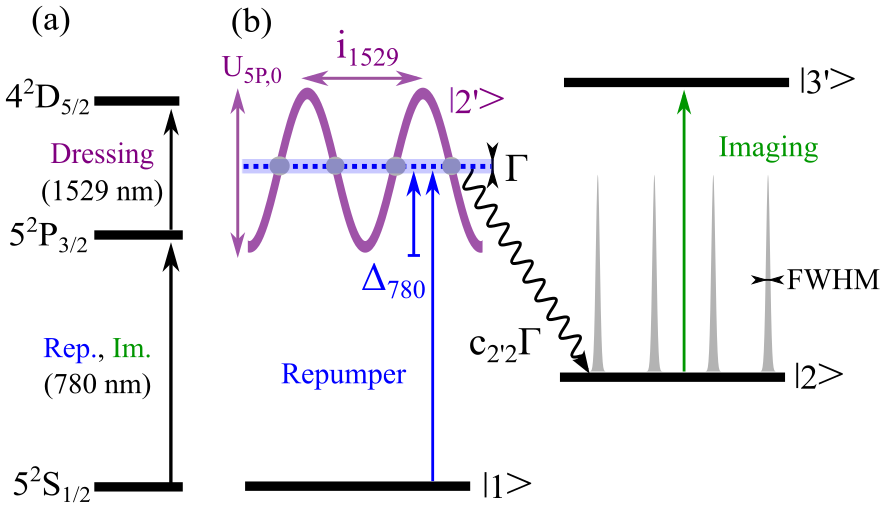
Figure 1: (a) Relevant three levels ⁸⁷Rb fine structure. (b) A three-level system with an optically dressed excited state using a 1529 nm lattice probed with a repumper at a detuning $\Delta_{780}$ and imaged on a cycling transition.

The detuning of the 780 nm laser with respect to the bare hyperfine state and the spatially-dependent saturation parameter are:

$$\Delta(x)=\Delta_{780}-\Delta_{\text{LS}}(x),$$ (2)

and,

$$s(x)= \frac{s_{0}}{1+4\Delta(x)^{2}},$$ (3)

where $\Delta_{780}=\omega_{780}-\omega_{0}$ is the bare detuning, $\Delta_{\text{LS}}(x)=\left(U_{\text{5P}}(x)-U_{\text{5S}}(x)\right)$ is the differential light shift between the ground and excited states, $U_{5S}(x)$ is the potential of the ground state which is small compared to the excited state light shift. The saturation parameter for the repumper transition is $s_{0}=I_{780}/I_{\text{sat,rep}}$, where $I_{780}$ is the intensity of the repumper beam and $I_{\text{sat,rep}}$ is the saturation intensity of the optical transition. In Appendix IV.2, we give the multi-level structure of ⁸⁷Rb and justify the choice of a three-level system (3LS) model to describe the population transfer from $\ket{1}$ to $\ket{2}$.

The point spread function (PSF), defined in our system as the spatially dependent population transferred in $\ket{2}$ ($\rho_{22}(x)$), is derived from the time evolution of the density matrix $\rho$ of the 3LS [11]. We focus on slow dynamics ($t\gg\Gamma$) where the adiabatic approximation is applied which assumes that the coherences are always in equilibrium with respect to the populations ($\dot{\rho}_{12^{\prime}}\approx 0$). In this case, the 3LS density matrix evolution simplifies to rate-equations:

$$\frac{d}{dt}\begin{pmatrix}{\rho_{11}}\\ {\rho_{2^{\prime}2^{\prime}}}\\ {\rho_{22}}\\ \end{pmatrix}=\begin{pmatrix}-\frac{s\Gamma}{2}&\frac{s\Gamma}{2}+c_{2^{\prime}1}\Gamma&0\\ \frac{s\Gamma}{2}&-\frac{s\Gamma}{2}-\Gamma&0\\ 0&c_{2^{\prime}2}\Gamma&0\\ \end{pmatrix}\begin{pmatrix}\rho_{11}\\ \rho_{2^{\prime}2^{\prime}}\\ \rho_{22}\\ \end{pmatrix}.$$ (4)

where $c_{2^{\prime}1}=1/2$ (resp. $c_{2^{\prime}2}=1/2$) are the normalized decay rates from $\ket{2^{\prime}}$ to $\ket{1}$ (resp. $\ket{2}$) due to spontaneous emission at a rate $\Gamma$.

An analytical solution of Eq. (4) is obtained by a diagonalisation method using symbolic computations. Starting from the initial state $\rho_{11}(t=0)=1$, the population of the state $\ket{2}$ at time $t$ is given by:

$$\rho_{22} =1-\frac{\Lambda_{-}}{\Lambda_{-}-\Lambda_{+}}e^{\Lambda_{+}t}-\frac{\Lambda_{+}}{\Lambda_{+}-\Lambda_{-}}e^{\Lambda_{-}t},$$ (5)

where $\Lambda_{\pm}=-{\Gamma}/{2}\left(1+s\pm\sqrt{1+2sc_{2^{\prime}1}+s^{2}}\right)$ correspond to non-zero eigenvalues.

In the low saturation limit $s_{0}\ll 1$ and including the spatial dependence of the saturation parameter $s(x)$, Eq. (5) simplifies to:

$$\rho_{22}(x)=1-e^{-c_{2^{\prime}2}\Gamma t\frac{s_{0}}{2}\frac{1}{1+s_{0}+4\Delta^{2}(x)}}.$$ (6)

For long pulse durations verifying $s_{0}\Gamma t\gg 1$ and for well-resolved fringes such that $\Gamma/U_{\text{5P,0}}\ll 1$, we can compute the full-width at half maximum of Eq. (6) for the two following limit cases:

• At the bottom of the modulation where $\Delta_{780}=0$:

  $$\text{FWHM}_{\text{bot}} =\sqrt{2}\left(\frac{\Gamma}{U_{\text{5P,0}}}\right)^{1/2}\frac{i_{1529}}{\pi}\left(\frac{c_{2^{\prime}2}\Gamma s_{0}t}{2\ln(2)}\right)^{1/4}.$$ (7)

• At the middle of the modulation where $\Delta_{780}=U_{\text{5P,0}}/2$:

  $$\text{FWHM}_{\text{mid}} =\frac{\Gamma}{U_{\text{5P,0}}}\frac{i_{1529}}{\pi}\left(\frac{c_{2^{\prime}2}\Gamma s_{0}t}{2\ln(2)}\right)^{1/2}.$$ (8)

As detailled in the next section, for our experimental implementation, Eq. (7) and (8) yield spatial widths smaller than the diffraction limit ($\lambda/2=390$ nm).

III Results

In the following, in III.1 we introduce the experimental setup used to produce and image the atomic clouds. Then, in III.2 we consider the case of cigar-shape thermal atomic cloud and a 1529 nm lattice that can be resolved by our imaging system. To validate our model, we measure the number of atoms transferred into the state $\ket{2}$ and compare it to the expected atom number deduced from our model. Finally, in III.3 we consider a Bose-Einstein Condensate loaded into a 1D lattice with a spacing smaller than the diffraction limit and we apply our method to image the longitudinal atomic density.

III.1 Cold atom apparatus

We prepare an atomic cloud of ⁸⁷Rb in state $\ket{1}$ using a hybrid trap composed of a magnetic trap compensating the gravity field and a crossed dipole trap (DT1, and DT2) [12]. Evaporative cooling is performed to produce either a thermal cloud or a BEC.

As shown in Figure 2 and 4, the 1529 nm lattice intensity is generated by the interferences of co- or counter-propagating laser beams with linear polarization aligned along $z$ which is set as the quantization axis. A $\pi$-polarized repumper pulse transfers the atoms to the state $\ket{2}$ which is imaged using a cycling transition. The repumper and imaging beam powers are monitored for each experimental runs from which the saturation parameters are computed.

We use a high numerical aperture absorption imaging system with a resolution limit of 1.3 µm. An image with atoms $I_{\text{at}}$, a reference image $I_{\text{noat}}$ of the imaging beam and an image for the background $I_{\text{back}}$ are acquired to compute the transmission $T=(I_{\text{at}}-I_{\text{back}})/(I_{\text{noat}}-I_{\text{back}})$ and the optical density $b=-\alpha\ln(T)+s_{\text{im}}(1-T)$ where the saturation parameter for the imaging beam is set at $s_{\text{im}}=1$.

For accurate atom number measurements, it has been crucial to calibrate the reduction factor $\alpha$ of the scattering cross-section which scales linearly with the optical density (OD) [13, 14]. In [13], we measured $\alpha(b)=\alpha_{0}+\beta b$ where $\alpha_{0}=1.17$ and $\beta=0.255$. Using this correction, the optical density is reformulated as $b={(-\alpha_{0}\ln(T)+s_{\text{im}}(1-T))}/{(1+\beta\ln(T))}$. Finally, the experimental atom number $N_{\text{tot}}=\iint b(x,y)dxdy/\sigma_{0}$ is computed using the scattering cross-section of a $\sigma^{-}$-polarized probe ($\sigma_{0}=2.907.10^{-9}$ cm²).

III.2 Characterization of the subwavelength PSF

For this experiment, we prepare and characterize by time-of-flight an initial thermal cloud containing $N_{0}=1.03(16).10^{5}$ atoms in $\ket{1}$ at a temperature of 169(10) nK, just above the condensation threshold. The cloud is trapped and compressed solely in DT2, creating a cigar-shape elongated along $y$. The atomic density is then homogeneous over a few 1529 fringe periods ($i_{1529}=8.3$ µm). An homogeneous magnetic bias of 280 mG along $z$ define the quantization axis. The maximum density at the cloud center is $1.8\times 10^{19}$ at/m³, giving an optical density of 31. To avoid high OD distorsion of atom number counting, we reduce the OD using coherent micro-wave (MW) transfer between the states $\ket{1}$ and $\ket{2}$ with transfer probability function $P(t_{\text{MW}})=P_{m}\sin^{2}(\pi t_{MW}/T_{MW})$, where $T_{MW}=56$ µs is the period and $P_{m}=0.96$ the maximum probability. A first MW $\pi$-pulse transfers all atoms from $\ket{1}$ to $\ket{2}$ and is followed by a short optical repumper pulse that empties the ground state $\ket{1}$. A second MW pulse of duration $t_{\text{MW}}=8$ µs is used to transfer a controlled population back into $\ket{1}$ and a cooler pulse pushes away the remaining atoms in $\ket{2}$. This sequence reduces the maximum optical density down to 6. In this configuration, the measured in situ cloud widths are $\sigma_{y}=64$ µm and $\sigma_{x}=2.4$ µm. The subwavelength imaging method described in section II is then performed on this thermal sample.

In the co-propagating case depicted in figure 2a, the lattice period is $i_{1529}=8.3$ µm. At mid-fringe, the clouds are separated by 4.15 µm which is well resolved by our microscope objective. This allows us to estimate the excitation size using both the well known atomic density and the measure of the number of transferred atoms $N_{exp}$. We additionally compute theoretically the expected atom number $N_{th}$ without any adjustable parameter by integrating the repumped fraction $\rho_{22}(y)$ over a width of one interfringe:

$$N_{\text{th}}= \frac{P(t_{\text{MW}})N_{0}}{\sqrt{2\pi}\sigma_{y}}\int_{0}^{i_{1529}}\rho_{22}(y)dy.$$ (9)

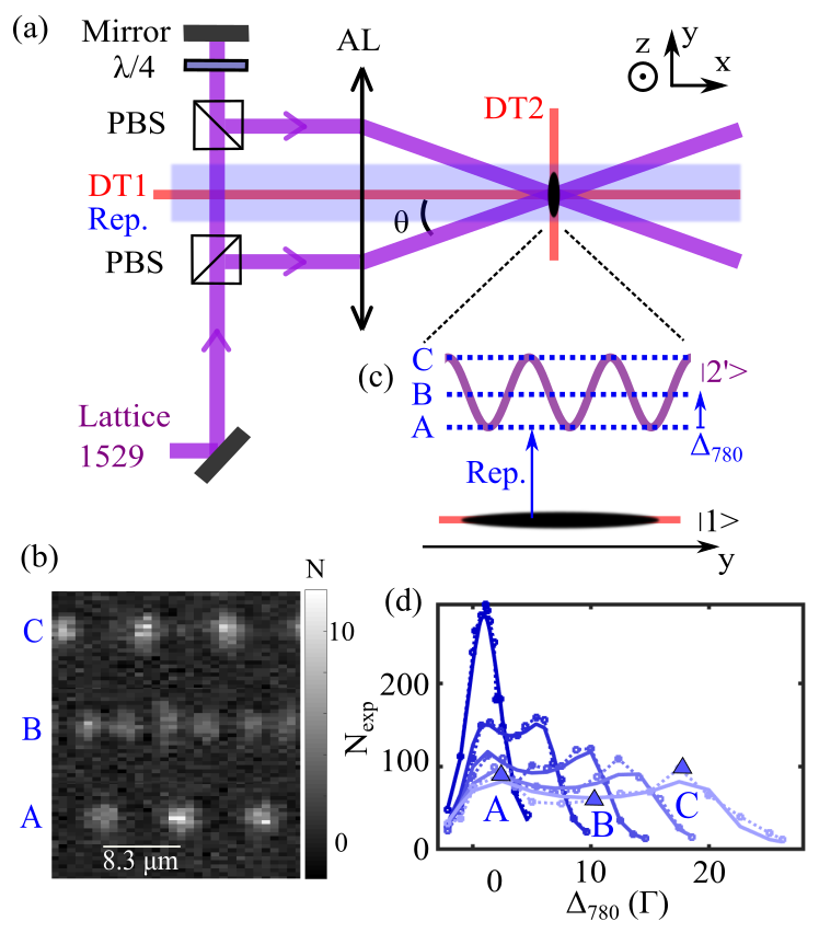
Figure 2: (a) Optical setup for the generation of the 1529 nm lattice. (b) Zoom on the ground state $\ket{1}$ with a homogeneous atomic cloud and the excited state $\ket{2^{\prime}}$. (c) 2D images of repumped atom numbers corresponding to the light blue curve on (d) which is the integrated atom number per interfringe (dashed lines with circles) for $U_{\text{5P,0}}$ of $2.5\Gamma$ (dark blue), $7.2\Gamma$, $11.6\Gamma$, $15.8\Gamma$ and $21\Gamma$ (dark blue), and fits (solid lines) with Eq. (9) where the free parameters are the light shift and the total atom number.

Fig. 2b shows in situ images of the atom number per pixel for three values of the repumper detuning ($\Delta_{780}=0,U_{\text{5P,0}}/2,U_{\text{5P,0}}$) for an excited state light shift of $U_{\text{5P,0}}=21\Gamma$. These images correspond to a tomography of the excited state. The number of atoms in one fringe ($N_{\text{exp}}$) is obtained by integrating the atomic density over one fringe. Figure 2c and d show the number of transferred atoms as a function of the repumper frequency for various excited state light shift. The points A, B, C corresponds respectively to the bottom, middle and top of the 1529 nm lattice. The width from the points A to C is a measure of the light shift and exactly matches with theoretical computations (see Appendix IV.1). The FWHM of Eq. (6) can be accurately computed with no free parameters and gives the expected atom number $N_{\rm th}$ in Eq. (9) that can be directly compared to the experimentally measured one $N_{\rm exp}$.

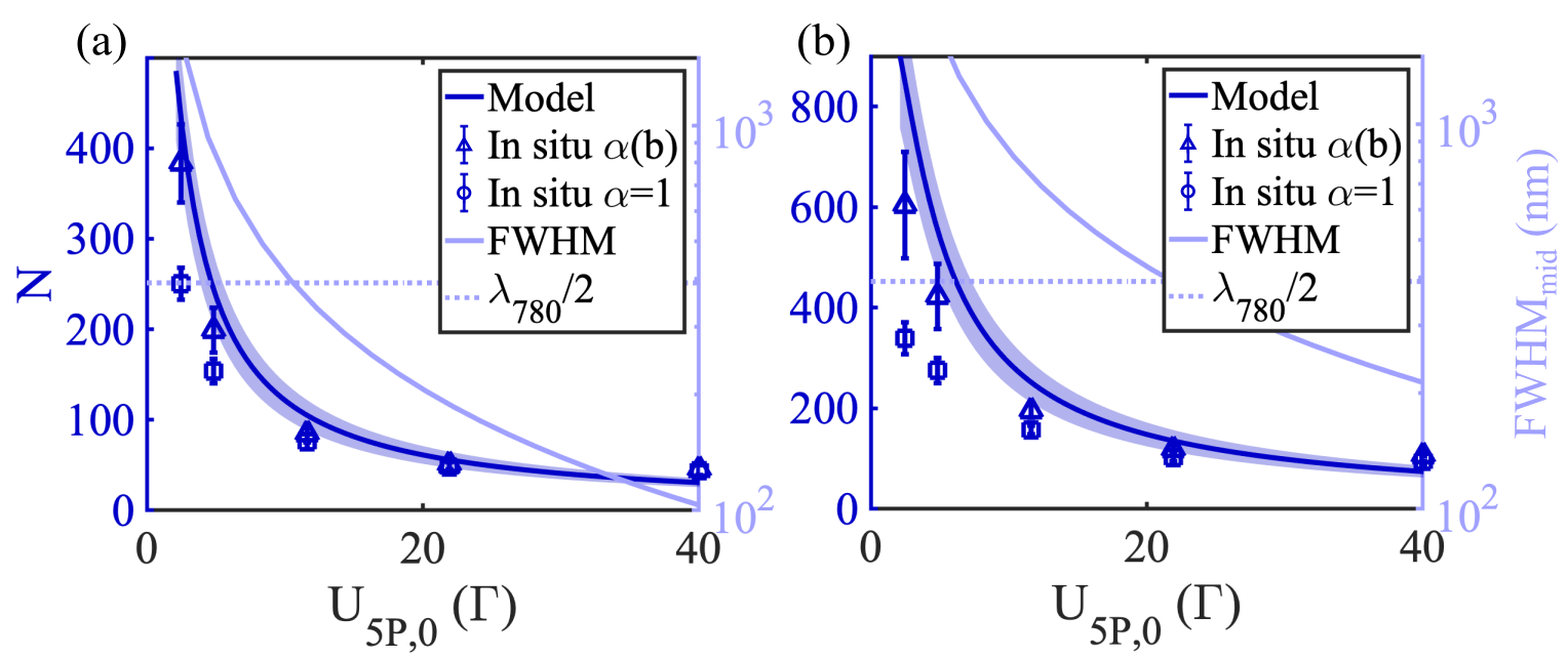
Figure 3: Atom number per unit of interfringe as a function on the light shift on the excited state $\ket{2^{\prime}}$ when $\Delta_{780}=U_{\text{5P,0}}/2$. The expected atom numbers is computed from the 3LS model with time-of-flight mesureaments (solid line), or in situ with $\alpha=1$ (dotted) and $\alpha=\alpha(b)$ (dashed lines). The resolution corresponds to the full-width at half maximum given by Eq. (8). The repumper saturations are (a) $s_{0}=0.022$, $t=8$ µs and (b) $s_{0}=0.063$, $t=12$ µs.

Fig. 3 shows the atom numbers $N_{\text{th}}$ and $N_{\text{exp}}$ as a function of the light shift amplitude $U_{\text{5P,0}}$ for two repumper saturations. The saturation and duration of repumper have been chosen such that the number of photons scattered on the repumper transition varies from 1 to 10 with either $s_{0}=0.022$ with $t=8$ µs or $s_{0}=0.063$ with $t=12$ µs. We see that using the correct atomic scattering cross-section ($\sigma_{0}/\alpha(b)$) leads to a very good agreement between the experimental and theoretical atom numbers $N_{\text{exp}}(\alpha(b))\approx N_{\text{th}}$. In comparison, we show the case of uncorrected data ($\alpha=1$) and we see that $N_{\text{exp}}(\alpha=1)<N_{\text{th}}$ in the low light shift limit which is where the transferred population $\ket{2}$ is the largest and the multiple scattering effects are the strongest [13]. For large light shifts ($U_{\rm 5P,0}=40\Gamma$), we detect more atoms than the model predicts. We attribute this discrepancy to the coupling of the repumper to other hyperfine excited states and to state mixing effects which are not included in the 3LS model.

The agreement of experimental and theoretical atom numbers confirms the validity of our model. As a result, we show the associated spatial resolutions given by Eq. (8) on Fig. 3a,b (right axis). For a large lattice spacing of $8.3\ \mu m$, we reached a FWHM of the repumped fraction of 100 nm which is smaller than the diffraction limit of $\lambda/2=390$ nm. This resolution being inversely proportional to the lattice spacing, it is expected to gain a factor $8.3/0.77=10.8$ by using counter-propagating beams.

III.3 PSF applied to a 1D lattice

In this section, we apply our method to image the longitudinal atomic density of a 1D optical lattice. For that purpose, the atoms are evaporated in an hybrid trap with a single dipole beam (DT1) to reach the Bose-Einstein Condensation with $2\times 10^{5}$ atoms. After compression of DT1, the trap frequencies are ($15,160,160$)Hz along ($x,y,z$). The atoms are then loaded in a 1064 nm lattice which is adiabatically ramped up from 0 to 40$E_{r}$, with $E_{r}$ the recoil energy at 1064 nm. The lattice depth has been characterized at the atom position using Kapitza-Dirac scattering [15, 16]. The magnetic gradient is then removed and a constant magnetic bias of 280 mG is set along $z$ before compressing the lattice up to 1000$E_{r}$. The width of the ground state wavefunction is given by the harmonic oscillator width $a_{\text{HO}}=\sqrt{\hbar/(m\omega)}$ where $\omega=2\sqrt{sE_{r}^{2}}/\hbar$ is the trap frequency and $s$ the lattice depth in recoil energy units. The standard deviation (std) of the atomic density along $x$ is therefore expected to be equal to $\sigma_{x}=a_{\text{HO}}/\sqrt{2}=21.2$ nm. Along $y$-direction, we experimentally measured a width $\sigma_{y}=$ 6 µm. The potential is spherically symmetric about $x$, we can then assume $\sigma_{z}=\sigma_{y}$.

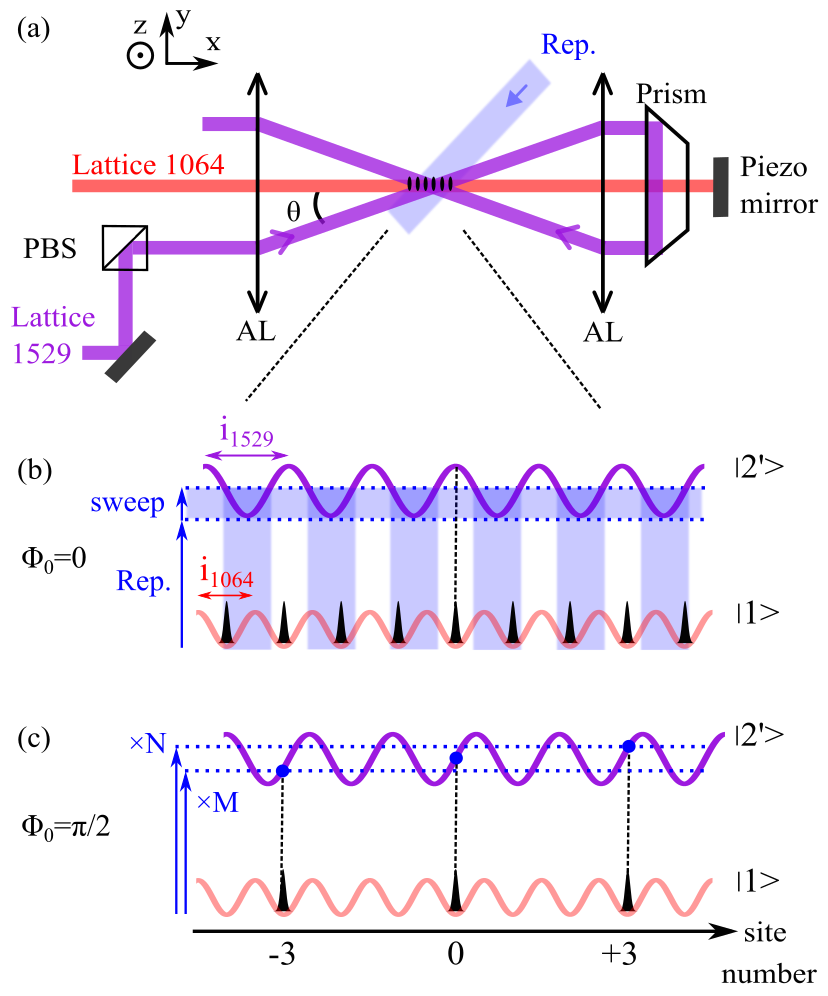
Figure 4: (a) Optical setup for the generation of the 1529 nm and 1064 nm lattices. (b) The two lattices with a relative phase $\Phi_{0}=0$. The blue shaded area corresponds to a sweep of the repumper frequency during the coarse cleaning of the lattice. (c) The two lattices with a relative phase $\Phi_{0}=\pi/2$. $M$ (resp. $N$) corresponds to the number of repumper pulses at specific frequency for the fine cleaning of the -3 (resp. +3 sites.

The ground state lattice with a period of $i_{1064}=\lambda_{1064}/2=532.23$ nm is formed by two counter-propagating beams (see Fig. 4a), yielding a ground state trapping potential given by:

$$U_{\text{5S}}(x)= U_{\text{5S,0}}\cos^{2}\left(\frac{k_{1064}}{2}x+\frac{\Phi_{0}}{2}\right),$$ (10)

where $k_{1064}=2\pi/i_{1064}$ is the lattice wavevector and $\Phi_{0}$ is the relative phase between the 1529 nm and the 1064 nm lattices. As shown in Fig. 4 b, , if $\Phi_{0}=0$ then both lattice extremum coincide for a central site, while if $\Phi_{0}=\pi/2$, the same central site is aligned at mid fringe of the 1529 nm lattice. The relative phase between the two lattices is controlled by a piezo stack that moves the reflecting mirror of the 1064 nm lattice. (see Appendix IV.3).

The 1529 nm lattice is generated along the 1064 nm lattice by reflecting a 1529 nm beam with a prism with an angle $\theta$ such that the interfringe is $i_{1529}={\lambda_{1529}}/{(2\cos(\theta))}$. Due to the different 1064 nm and 1529 nm lattice periodicities, a perfect commensurability is obtained for a given number of sites $n_{1064}$ at 1064 nm for the ground state and $n_{1529}$ at 1529 nm for the excited state:

$$n_{1529}i_{1529}=n_{1064}i_{1064}.$$ (11)

This gives sets of angles for $\theta$ for which the commensurability is obtained:

$$\theta=\acos\left(\frac{n_{1529}\lambda_{1529}}{n_{1064}\lambda_{1064}}\right).$$ (12)

Due to experimental mechanical constraints, the only accessible angle in our setup is $\theta=5.92^{\circ}$ for which we have $n_{1064}=13$ and $n_{1529}=9$. We have therefore a super-lattice period of 6.9 $\mu$m where every 13 interfringes of the 1064 nm lattice, the atoms will see exactly the same modulation of the 1529 nm lattice in the excited state. This super-lattice period is large and can be resolved easily by our microscope objective which enables the superresolution of the lattice sites.

To demonstrate the performances of the method, we now aim at measuring the standard deviation (std) of a single site that we will label site number 0. We start by preparing that single site in two steps. In a first step, we perform a coarse cleaning stage in which all sites except sites 0 and $\pm 3$, as indexed in Fig. 4b, are repumped. For that purpose, we spatially shift the excited state using a 529 nm modulation of $U_{\text{5P,0}}=17\Gamma$ and repump the atoms while sweeping in 10 ms the detuning of the repumper from $\Delta_{780}=0.4U_{\text{5P,0}}$ to $U_{\text{5P,0}}$ at a saturation of $s_{0}=2\times 10^{-3}$. All repumped atoms are then pushed away with a cooler pulse. In a second step, the piezo is ramped in 100 ms by a distance of $i_{1529}/4$ to align the site 0 onto a slope of the 1529 nm modulation as shown on Fig. 4c. The sites +3 (resp. -3) are cleaned using $N$ (resp. $M$) short repumper pulses at $\Delta_{780}=3\Gamma$ (resp. $\Delta_{780}=U_{\text{5P,0}}-3\Gamma$). Finally, the atomic density is imaged by varying the relative phase $\Phi_{0}$ and applying a last repumper pulse of detuning $\Delta_{780}=U_{\text{5P,0}}/2$, saturation $s_{0}=0.02$ and duration $t=16$ µs. The corresponding atomic densities are shown on Fig. 5a,b,c. Each curve is fitted by a Gaussian function from which the central position and std are shown on Fig. 5d,e.

As $M$ increases while $N=0$ (Fig. 5a), cleaning only the sites $-3$ shifts the wavepackets to the right after which it remains stable. In that case we can consider that the $-3$ site is empty. As the site $0$ is centered at the middle of the excited state modulation, the sites $\pm 3$ would be resonant exactly at $(3i_{1064}-2i_{1529})=60$ nm away from that central position. Therefore, for equal initial populations in the sites $-3,+3,0$, the central position should shift by at maximum $30$ nm. However, during the coarse cleaning stage, the $\pm 3$ sites are closer from resonance than the site $0$ and the repumper therefore induce more scattering on these sites and reduce more their population. These unequal populations would lead to a smaller shift of the central position. From numerical simulations (see Appendix IV.4), the experimental measured shift of about 20 nm is reproduced for relative populations of 0.6 in the sites $\pm 3$.

As both $M$ and $N$ increase, the Gaussian std decreases as expected as $\pm 3$ sites get cleaned (Fig. 5e). At minimum, the expected std should be 27 nm which corresponds to the convolution of the atomic density and the point spread function. We measured a std of $45\pm 5$ nm which is slightly larger than the expected one. This expected width limit (dashed line) corresponds to the case of a perfect alignment of the two lattices. It is however very sensitive to the relative angle between the lattice wave-vectors. In Appendix IV.5, we computed the effective std $\tilde{\sigma}_{x}$ after adding a rotation angle $\eta_{y}$ about the $y$-axis between the two lattices. We showed that in the small angle limit the std is given by $\tilde{\sigma}_{x}=\sigma_{x}\sqrt{1+\eta_{y}^{2}(\sigma_{y}/\sigma_{x})^{2}}$. For only $0.3^{\circ}$ (dash-dotted line in Fig. 5e), the calculated widths overlap with the experimental data.

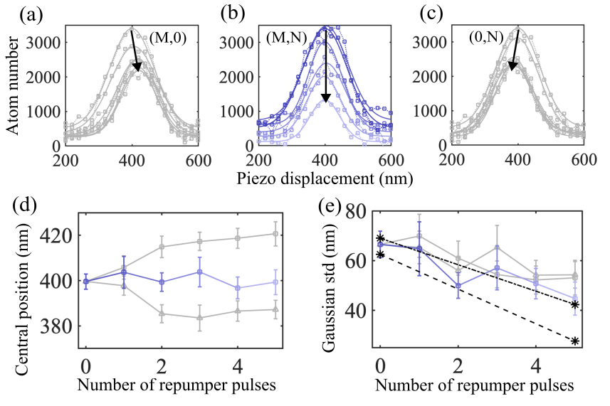
Figure 5: (a), (b), (c) Wavepacket density imaging by scanning the piezo mirror. The arrow indicates an increasing number of cleaning pulses of respectively $(M,0)$, $(M,N=M)$ and $(0,N)$ where $M$ and $N$ varies from 0 to 5 pulses. Dotted lines with squares are the data and the lines are Gaussian fits from which the central position (d) and width (e) are extracted. Errorbars are fit errors. In (e), the two star points with a dashed black line (resp. dash-dotted black line) shows the theoretical widths for $\eta_{y}=0^{\circ}$ (resp. $\eta_{y}=0.3^{\circ}$).

IV Conclusion

In this work, we used atoms as a local probe of their electromagnetic environment. We have demonstrated that excited state energy shifts were a versatile and well controlled solution to manipulate atomic transition frequencies over very short distances. We first applied the method in an optically resolved situation where we have demonstrated an excitation length around 100 nm. This resolution is well explained and quantitatively correspond to a model accounting for the internal state dynamics of a 3LS. We emphasize that the excitation length estimate relies on an absolute measurement of atom numbers. The quantitative match between the model and experimental data for large optical depths (low modulation depth) requires to account for a non-negligible reduction of the scattering cross section that was characterized in [13]. In the non-optically resolved limit (section III.3), the slope of the excited state energy was increased by the ratio of lattice spacing $8.3/0.768\approx 10.8$ which also corresponds to the reduction factor of the excitation length. We have used this improved resolution to image a strongly compressed atomic density. The expected std of $27$ nm given by the convolution of the atomic density ($21$ nm) and the point spread function is smaller than the measured width of $45\pm 5$ nm. We believe that the discrepancy is certainly explained by a slight lattice misalignment (see Appendix Appendix). The current experimental and numerical simulations have been performed for ⁸⁷Rb atoms. It can straightforwardly be extended to other alcaline species with large excited state hyperfine splittings such as Cesium atoms. For alcalines with lower excited state splitting, the method could be extended in the large field limit that would result in a mixing of the strongly shifted excited states, requiring to redefine the proper eigenbasis. With our method, the resolution depends both on the excited state shift and on the excited state linewidth, making it favorable for atomic species with narrow transitions, such as Strontium atoms for instance. The long living excited states shift can be controlled via the strong dipole coupling of the triplet states to the excited singlet states. Similar arguments apply for other species with long living excited states such as Dysprosium atoms.

Appendix

In the Appendix IV.1 we compare the experimental light shifts induced by the 1529 nm lattice to theoretical computations. In Appendix IV.2 we describe the three-level system model that is used to compute the point spread function. In Appendix IV.3 we show how the piezo stack controlling the 1064 nm is calibrated. Finally, we simulate the wavepacket microscopy sequence in the 1064 nm lattice to study the influence of experimental imperfections on the central position of the wavepacket in IV.4 and its associated width in IV.5.

IV.1 Light shifts at 1529 nm

The light shifts induced by the 1529 nm laser are computed by diagonalising the total Hamiltonian composed of the AC Stark Hamiltonian and the hyperfine Hamiltonian [11].

To compute the light shifts for a far-off-resonance laser, the counter-rotating term of the atom-field interaction has to be included. As both terms oscillate rapidly compared to each other, both light shifts computed independently from each other can be added after their respective diagonalisation in their own rotating-frame.

The numerical computations of the light shifts of the state $5P_{3/2}$ with a laser at exactly 1529.36098 nm includes the following states: $5S_{1/2}$, $5P_{1/2}$, $5P_{3/2}$, $6P_{1/2}$, $4D_{3/2}$ and $4D_{3/2}$. The main transitions that contribute to the light shifts are $5P_{3/2}$ to $4D_{5/2}$ at 1529.366 nm with dipole moment of $10.899ea_{0}$ and $5P_{3/2}$ to $4D_{3/2}$ at 1529.262 nm with dipole moment of $3.628ea_{0}$ where $e$ the electron charge and $a_{0}$ the Bohr radius. Atomic parameters can be found in [17], [18]. Our 1529 nm laser mainly drives the transition between $5P_{3/2}$ and $4D_{5/2}$ depicted on Fig. 1a. The theoretical light shift is ultimately obtained by the knowledge of the intensity of the 1529 nm laser beams. The power is locked and the waists are measured using a tomography technique [19]. The 1529 nm resonance is found by a spectroscopic scan onto the atoms.

We compared this theoretical description of the light shift with the experimental realizations on Fig. 6 for the homogenous cloud configuration. 5 repetitions of a tomographic curve are measured, from which the light shifts are obtained by fitting the atom number with Eq. (6). Both agree which enables us to precisely compute the spatial resolutions with Eq. (8) as the light shift is an input parameter.

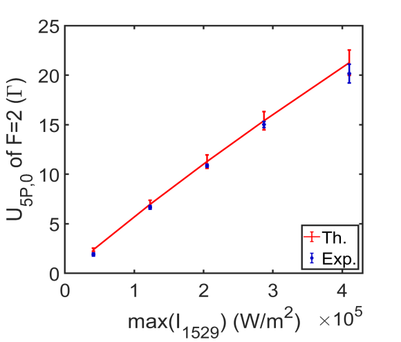
Figure 6: Experimental light shifts obtained from a tomographic measurements compared to the theoretical shifts computed from the knowledge of the waists, frequency and powers of the 1529 nm beams. Errorbars correspond to the waist uncertainty for the theoretical model and to the standard deviation over 5 realizations for the experimental data.

IV.2 3LS repump model for ⁸⁷Rb

Fig. 7 shows the effective 3LS that we consider to model the point spread function based on the multi-level structure of ⁸⁷Rb.

The differential light shifts between the $m_{F}$ states of $F^{\prime}=2$ for a $\pi$-polarized 1529 nm laser are much lower than the atomic linewidth $\Gamma/2\pi=6.066$ MHz. As a result, there is no dark state in the hyperfine ground state $F=1$ as all $m_{F}$ states can be locally coupled to the excited state. We numerically checked that taking all the states coupled by $\pi$-transitions or approximating it as a two-level system leads to the same population transfer. Therefore, we treat the multi-level repumper transition as the two-level system: $\ket{1}$ and $\ket{2^{\prime}}$ (blue levels in Fig. 7). For this two-level system, as the atom is initially prepared in $\ket{5^{2}S_{1/2},F=1,m_{F}=-1}$, we include in the saturation parameter the coupling strength of the transition between $\ket{5^{2}S_{1/2},F=1,m_{F}=-1}$ and $\ket{5^{2}P_{3/2},F^{\prime}=2,m_{F}=-1}$ of $-\sqrt{1/8}$ [20] which leads to a saturation intensity of $I_{\text{sat,rep}}=6.67$ mW/cm².

We ignore the coupling from $\ket{1}$ to the excited state $\ket{5^{2}P_{3/2},F^{\prime}=1,m_{F}=-1}$ as it is $26\Gamma$ away from $\ket{2^{\prime}}$ which is smaller that the 1529 nm induced light shifts of the experiment.

The population in $\ket{1}$ is transferred via absorption/spontaneous emission cycles into $F=2$ and remains there: we treat all $m_{F}$ state of $F=2$ as a single state $\ket{2}$.

Finally, the population in $\ket{2}$ is measured by absorption imaging using a circularly polarised laser tuned on the cycling transition from $\ket{5^{2}S_{1/2},F=2,m_{F}=-2}$ to $\ket{5^{2}P_{3/2},F^{\prime}=3,m_{F}=-3}$.

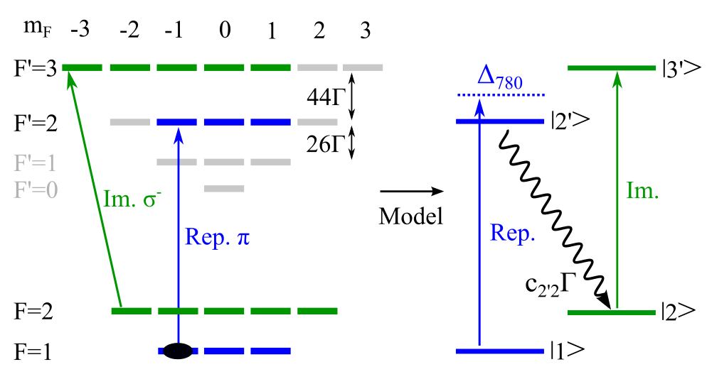
Figure 7: ⁸⁷Rb D₂ transition hyperfine structure ($5^{2}S_{1/2}$ to $5^{2}P_{3/2}$) and its approximation as a 3LS for the repumper transition and as a 2LS for the imaging transition.

IV.3 Piezo displacement calibration

The piezo stack controlling the position of the 1064 nm lattice is calibrated by measuring the displacement of on atomic fringes on a camera as a function of the piezo drive as shown on Fig. 8. These fringes are obtained after loading the 1064 nm lattice, turning on the 1529 nm lattice, repumping the atoms using $\Delta_{780}=0\Gamma$ and imaging them by aborption imaging. The piezo displacement axis is ultimately calibrated by knowing that two consecutive fringes along the site number axis is equal to $13i_{1064}=6.9$ µm. Along the piezo displacement axis, a displacement of exactly $i_{1064}$ gives the same fringe position due to the lattice periodicity. Note that the fringe visible around the site n${}^{\circ}0$ at a displacement of $0.6i_{1064}$ corresponds to the site n^∘-1 which is resonant.

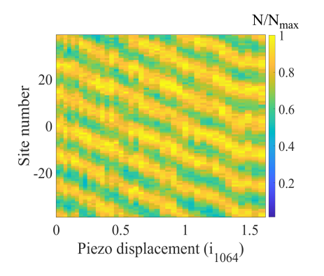
Figure 8: Projection along the $x$-axis of normalized atom numbers after repumping atoms in the 1064 nm lattice with $\Delta_{780}=0$, $s_{0}=0.02$ and $t=8$ µs in a modulation of $U_{\text{5P,0}}=16\Gamma$ as a function the camera axis ($y$-axis) and the relative phase $\Phi_{0}$ ($x$-axis) between the two lattices.

IV.4 Central position shifts

We numerically compute the position shift of the imaged wavepacket by simulating the total repumped fraction for different relative populations in the sites $\pm 3$ compared to the population in site 0. We scan numerically the relative phase between the lattices given the initial atomic density and knowing the point spread function $\rho_{22}(x)$, we compute the repumped populations. Then, we fit the resulting wavepackets with a Gaussian function to extract the central position. We see on Fig. 9 that for approximately populations of 0.6, the wavepacket shifts by $\pm 20$ nm which corresponds to the experimental data. We checked that residual angles as described in Appendix IV.5 do not shift significantly the position of the wavepacket.

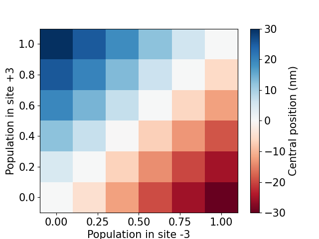
Figure 9: Central position shift of the wavepacket as a function of relative initial populations in the sites $\pm 3$.

IV.5 Width broadening by lattice misalignment

The atomic density in the ground state lattice site is characterized by the widths $\sigma_{x}\ll\sigma_{y,z}$ and $\sigma_{y}=\sigma_{z}$. Let us consider a 2D Gaussian atomic density in a rotated frame $(x^{\prime},i^{\prime})$ by an angle $\eta_{i}$ such that:

$$n(x^{\prime},i^{\prime})=e^{-\frac{x^{\prime 2}}{2\sigma_{x}^{2}}-\frac{i^{\prime 2}}{2\sigma_{i}^{2}}}.$$ (13)

The rotated frame is expressed in the intial frame by

$$\begin{pmatrix}x^{\prime}\\ i^{\prime}\end{pmatrix}=\begin{pmatrix}\cos(\eta_{i})&-\sin(\eta_{i})\\ \sin(\eta_{i})&\cos(\eta_{i})\end{pmatrix}\begin{pmatrix}x\\ i\end{pmatrix},$$ (14)

where $i\in\{y,z\}$.

Integrating Eq. (13) over the direction $i$, using $\sigma_{y}\gg\sigma_{x}$ and considering the case of small angles $\eta_{i}\ll 1$, one can compute the linear atomic density:

$$n(x)=e^{-\frac{x^{2}}{2\tilde{\sigma}_{x}^{2}}},$$ (15)

where the effective width $\tilde{\sigma}_{x}$ is given in the main text.

It is clear that a rotation about $x$-axis does not lead to any broadening as the potential is symmetric.

In the case of a relative angle $\eta_{z}$ about the $z$-axis (Fig. 10), the projection of the repumped cloud along $y$ is shifted on the order of $\sigma_{y}$ which corresponds to an angle of 0.3°. Experimentally, the cloud shifts by less than a micrometer so we believe that $\eta_{z}$ does not contribute to a broadening. Note that other datasets shown shifts on the order of a few micrometers and we could minimized that shift by a better alignment of the counter-propagating 1529 nm beam.

The angle $\eta_{y}$ is difficult to estimate experimentally, as on one hand the $z$-direction is integrated by the imaging system so we do not have access to that spatial direction to look for a displacement of the projection, and on the other hand, a small displacement on the order of $\sigma_{x}$ is difficult to measure along $x$.

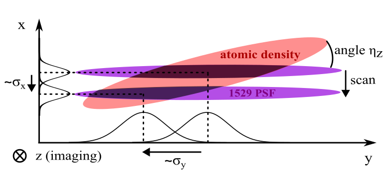
Figure 10: Schematics of the projection position shift of the repumped atomic cloud in the case of a relative angle $\eta_{z}$ between an atomic wavepacket and a 1529 nm point spread function plane.

As in Appendix IV.3, we perform a complete simulation of the measured wavepacket but we also include $\eta_{y}$ as a free parameter. We use the initial population in the $\pm 3$ sites that we found in Appendix IV.3. For this population, we numerically compute a width of 69 nm which matches with the experimental data of Fig. 5e in the main text. Then, we found that the experimental width after the second cleaning step can be explained by an angle $\eta_{y}=0.3^{\circ}$ which globally shifts the theoretical line towards larger widths.

Other sources of broadening could be consider in the case of perfect alignement. We ensured that the lattice laser frequencies do not drift significantly by frequency locking them on the same transfer cavity. Then, the initial phase at the atom position might also fluctuate over time due to room temperature changes. This would lead to an imperfect initial positionning of the site $0$ at the beginning of the first cleaning sequence and would cause an asymmetry in the measured wavepacket in the second cleaning step as either the $-3$ site or $+3$ site would be closer or further from resonance. Finally, the last repumper pulse can be shortened to durations smaller than the trap frequency period to avoid dynamical effects. We tried to use shorter repumper durations and did not see a narrower wavepackets which suggests that the dominating width broadening was due a residual angle, as in such a case, the dynamics in the trap along $x$ would be on longer timescales than along $x^{\prime}$.

References

- Schäfer et al. [2020] F. Schäfer, T. Fukuhara, S. Sugawa, Y. Takasu, and Y. Takahashi, Tools for quantum simulation with ultracold atoms in optical lattices, Nat. Rev. Phys. 2, 10.1038/s42254-020-0195-3 (2020).
- Mazurenko et al. [2017] A. Mazurenko, C. S. Chiu, G. Ji, M. F. Parsons, M. Kanász-Nagy, R. Schmidt, F. Grusdt, E. Demler, D. Greif, and M. Greiner, A cold-atom Fermi-Hubbard antiferromagnet, Nature 545, 10.1038/nature22362 (2017).
- Koepsell et al. [2020] J. Koepsell, S. Hirthe, D. Bourgund, P. Sompet, J. Vijayan, G. Salomon, C. Gross, and I. Bloch, Robust Bilayer Charge Pumping for Spin- and Density-Resolved Quantum Gas Microscopy, Phys. Rev. Lett. 125, 10.1103/PhysRevLett.125.010403 (2020).
- Nascimbene et al. [2015] S. Nascimbene, N. Goldman, N. R. Cooper, and J. Dalibard, Dynamic Optical Lattices of Subwavelength Spacing for Ultracold Atoms, Physical Review Letters 115, 140401 (2015).
- Tsui et al. [2020] T.-C. Tsui, Y. Wang, S. Subhankar, J. V. Porto, and S. L. Rolston, Realization of a stroboscopic optical lattice for cold atoms with subwavelength spacing, Physical Review A 101, 041603 (2020).
- Bellouvet et al. [2018] M. Bellouvet, C. Busquet, J. Zhang, P. Lalanne, P. Bouyer, and S. Bernon, Doubly dressed states for near-field trapping and subwavelength lattice structuring, Phys. Rev. A 98, 10.1103/PhysRevA.98.023429 (2018).
- Weitenberg et al. [2011] C. Weitenberg, M. Endres, J. F. Sherson, M. Cheneau, P. Schauß, T. Fukuhara, I. Bloch, and S. Kuhr, Single-spin addressing in an atomic Mott insulator, Nature 471, 10.1038/nature09827 (2011).
- Alberti et al. [2016] A. Alberti, C. Robens, W. Alt, S. Brakhane, M. Karski, R. Reimann, A. Widera, and D. Meschede, Super-resolution microscopy of single atoms in optical lattices, New J. Phys. 18, 10.1088/1367-2630/18/5/053010 (2016).
- Subhankar et al. [2019] S. Subhankar, Y. Wang, T.-C. Tsui, S. Rolston, and J. V. Porto, Nanoscale Atomic Density Microscopy, Phys. Rev. X 9, 10.1103/PhysRevX.9.021002 (2019).
- McDonald et al. [2019] M. McDonald, J. Trisnadi, K.-X. Yao, and C. Chin, Superresolution Microscopy of Cold Atoms in an Optical Lattice, Phys. Rev. X 9, 10.1103/PhysRevX.9.021001 (2019).
- Steck [2019] D. A. Steck, Quantum and atom optics, (2019).
- Lin et al. [2009] Y.-J. Lin, A. R. Perry, R. L. Compton, I. B. Spielman, and J. V. Porto, Rapid production of 87Rb Bose-Einstein condensates in a combined magnetic and optical potential, Phys. Rev. A 79, 10.1103/PhysRevA.79.063631 (2009).
- Veyron et al. [2022a] R. Veyron, V. Mancois, J.-B. Gerent, G. Baclet, P. Bouyer, and S. Bernon, Quantitative absorption imaging: The role of incoherent multiple scattering in the saturating regime, Phys. Rev. Res. 4, 033033 (2022a).
- Veyron et al. [2022b] R. Veyron, V. Mancois, J. B. Gerent, G. Baclet, P. Bouyer, and S. Bernon, Effective two-level approximation of a multilevel system driven by coherent and incoherent fields, Physical Review A 105, 043105 (2022b).
- Gadway et al. [2009] B. Gadway, D. Pertot, R. Reimann, M. G. Cohen, and D. Schneble, Analysis of Kapitza-Dirac diffraction patterns beyond the Raman-Nath regime, Opt. Express 17, 10.1364/OE.17.019173 (2009).
- Denschlag et al. [2002] J. H. Denschlag, J. E. Simsarian, H. Häffner, C. McKenzie, A. Browaeys, D. Cho, K. Helmerson, S. L. Rolston, and W. D. Phillips, A Bose-Einstein condensate in an optical lattice, J. Phys. B 35, 10.1088/0953-4075/35/14/307 (2002).
- Arora and Sahoo [2019] B. Arora and B. K. Sahoo, State-insensitive trapping of Rb atoms: Linearly versus circularly polarized light, Phys. Rev. A 99, 10.1103/PhysRevA.99.049901 (2019).
- Arora et al. [2007] B. Arora, M. S. Safronova, and C. W. Clark, Magic wavelengths for the np-ns transitions in alkali-metal atoms, Phys. Rev. A 76, 10.1103/PhysRevA.76.052509 (2007).
- Bertoldi et al. [2010] A. Bertoldi, S. Bernon, T. Vanderbruggen, A. Landragin, and P. Bouyer, In situ characterization of an optical cavity using atomic light shift, Opt. Lett. 35, 10.1364/OL.35.003769 (2010).
- Steck [2001] D. A. Steck, Rubidium 87 D line data, (2001).