Medial Skeletal Diagram: A Generalized Medial Axis Approach for Compact 3D Shape Representation

Abstract.

We propose the Medial Skeletal Diagram, a novel skeletal representation that tackles the prevailing issues around compactness and reconstruction accuracy in existing skeletal representations. Our approach augments the continuous elements in the medial axis representation to effectively shift the complexity away from the discrete elements. To that end, we introduce generalized enveloping primitives, an enhancement over the standard primitives in the medial axis, which ensure efficient coverage of intricate local features of the input shape and substantially reduce the number of discrete elements required. Moreover, we present a computational framework for constructing a medial skeletal diagram from an arbitrary closed manifold mesh. Our optimization pipeline ensures that the resulting medial skeletal diagram comprehensively covers the input shape with the fewest primitives. Additionally, each optimized primitive undergoes a post-refinement process to guarantee an accurate match with the source mesh in both geometry and tessellation. We validate our approach on a comprehensive benchmark of 100 shapes, demonstrating the compactness of the discrete elements and superior reconstruction accuracy across a variety of cases. Finally, we exemplify the versatility of our representation in downstream applications such as shape generation, mesh decomposition, shape optimization, mesh alignment, mesh compression, and user-interactive design.

1. Introduction

Geometric shape representations are fundamental to diverse areas of computer graphics and geometric modeling. Among them, the shape skeleton stands out as a powerful and intuitive tool for understanding and manipulating shapes, with a particularly broad range of applications including 3D reconstruction [Tang et al., 2019], shape segmentation [Lin et al., 2020], character animation [Baran and Popović, 2007], and shape correspondence [Wong et al., 2012]. As a prominent example among skeletal representations, the medial axis [Blum, 1967] is ubiquitous in shape approximation, simplification, and analysis tasks. The approximative counterpart, medial axis transform (MAT), comprises a discrete simplicial complex (termed medial mesh) and a continuous radius function defined on each vertex of the complex. Consequently, MAT enjoys many advantages including lower dimensionality than the original shapes, effective capture of components and protrusions, and preservation of homotopy [Lieutier, 2003].

Nonetheless, like most existing skeletal representations, the medial axis representation encounters an inevitable trade-off between the compactness of the skeletal structure and completeness of the reconstruction. The skeletal structure should ideally be as simple and compact as possible to allow for easy interpretation and modification. However, it is equally important to retain sufficient complexity to faithfully reconstruct all geometric details and features. Balancing such conflicting requirements poses a significant challenge. The excessive complexity hinders the application of medial axis to shape generation and interactive shape editing, which require a more compact skeleton but a complete representation. Numerous research efforts have been dedicated to simplifying the discrete part of the skeletal representation to enhance its manageability and visual cleanliness [Li et al., 2015; Dou et al., 2022; Lin et al., 2021; Tagliasacchi et al., 2016]. However, despite these advancements, the simplified skeleton is still bounded by excessively many elements with compromised reconstruction accuracy, resulting in degraded quality of the skeleton and a loss of geometric detail.

To conquer these limitations, we present a novel skeletal representation that significantly reduces the number of discrete elements while preserving the completeness characteristic of the medial axis. Our method stems from the insight that the complexity of the medial axis skeleton can be decimated by an augmented representation of the continuous elements. Discrete elements are often challenging to optimize due to their combinatorial nature, which results in severe computational bottlenecks. In contrast, continuous elements can be formulated and solved efficiently using off-the-shelf optimization frameworks.

Our versatile skeletal representation, named the medial skeletal diagram (MSD), extends the medial axis using generalized enveloping primitives. Compared with the uniform, linearly interpolated primitives used in the medial axis, our generalized enveloping primitives are non-uniform and nonlinearly interpolated. For example, the medial axis assumes consistent and uniform radii, whereas in our medial skeletal diagram, each medial sphere has varying radii along different directions. Such generalized primitives can effectively cover complex local regions, which in turn reduces the number of primitives required to represent a given shape. As a result, the medial skeletal diagram can represent arbitrary closed manifold surfaces, with the raw medial axis being a special case.

To construct a medial skeletal diagram for an arbitrary input, we start by building a forward procedure. This procedure takes a subset of points from the raw medial axis as its input and produces an MSD as its output. Utilizing restricted Voronoi diagrams (RVD) and restricted Delaunay triangulation (RDT), we determine the discrete skeletal structure based on the input set of points, which effectively ”remesh” the medial axis. Following this, generalized enveloping primitives are generated at each element of the discrete skeletal structure to align with the input mesh. With this established procedure, transforming a subset of medial axis points into a medial skeletal diagram, we then introduce an optimization pipeline. This pipeline is designed to identify the optimal subset of points, ensuring that the resulting medial skeletal diagram covers the input shape with the fewest necessary primitives. In the final stage, the optimized primitives undergo a refinement phase, aimed at achieving precise alignment with the target mesh in both its geometric form and tessellation.

The contributions of this paper are summarized as follows:

• We propose a novel 3D shape representation (in Sec. 4) that extends the medial axis approach using generalized enveloping primitives, enabling both compact skeletal structures and accurate representation for arbitrary closed manifold surfaces.

• We introduce a computational pipeline to construct the medial skeletal diagram from any given shape (in Sec. 5). Our pipeline find the best MSD which maximizes the coverage of the input shape with a minimal number of primitives. A subsequent refinement process precisely aligns optimized primitives with the target mesh, both in terms of geometry and tessellation.

• We validate the medial skeletal diagram on a benchmark of $100$ shapes to demonstrate the compactness of the skeleton and the completeness of the representation (in Sec. 6). Furthermore, we showcase the versatility and advantages of our representation in the context of shape optimization, shape generation, mesh decomposition, mesh alignment, mesh compression, and user-interactive design.

2. Related Work

Medial axis transformation.

MAT represents a 3D shape using thin-centered structures and is able to jointly describe shape topology and geometry. The rich history of MAT starts from early algorithms that employ seam tracing techniques to calculate the exact MAT for polyhedra [Milenkovic, 1993; Sherbrooke et al., 1996; Culver et al., 2004]. These exact algorithms primarily concentrate on simple shapes with up to $20$ faces. A significant amount of subsequent research has shifted towards approximated MAT, which is more suitable for practical applications [Amenta et al., 2001b; Pizer et al., 2003; Dey and Zhao, 2004; Chazal and Lieutier, 2005; Miklos et al., 2010; Sobiecki et al., 2014; Saha et al., 2016]. For a more comprehensive discussion, we refer the reader to survey papers by Pizer et al. [2003]; Tagliasacchi et al. [2016].

Curve skeletonization.

One type of shape representation relevant to our work is curve skeletons, which have been widely studied in rigging and interactive shape modeling [Borosán et al., 2012]. Traditional approaches compute curve skeletons following hand-crafted rules that encode geometric information. For instance, Ma et al. [2003] extract skeletons using radial basis functions. Sharf et al. [2007] apply deformable model evolution to capture the volumetric shape of an object for curve skeleton approximation. Au et al. [2008] compute the curve skeleton via mesh extraction. Livesu et al. [2012] use visual hulls to reconstruct curve skeletons. Mean curvature skeletonization [Tagliasacchi et al., 2012] creates curve skeletons by deploying mean curvature flow on the shape. Reeb graphs [Tierny et al., 2008] are also considered curve skeletons, which are constructed by tracing the isocontours of a given height function and contracting connected components into a single point. However, they are often suboptimal as skeleton junctions can be very close to the surface. Recently, Bærentzen and Rotenberg [2021] and Bærentzen et al. [2023] treat 3D shapes as spatially embedded graphs and compute curve skeletons using local operators. In shape modeling,  Bærentzen et al. [2014] use polar-annular mesh to obtain a co-representation of both the mesh and the curve skeleton. Pandey et al. [2022] obtain a curve skeleton from a sequence of face-loop modeling operations on a quad mesh. Although curve skeletons are well-suited for representing organic, articulated shapes, they often suffer from capturing large thin flat components, which are prevalent in CAD models. Our representation incorporates triangles and effectively captures large, flat regions with fewer elements.

Medial axis Simplification.

The medial axis representation is complete but sensitive to boundary noise. This has led to a large body of research on its simplification while preserving significant and stable parts. Angle-based filtering methods [Amenta et al., 2001a; Foskey et al., 2003; Dey and Zhao, 2002; Sud et al., 2005] consider the angle in MAT during simplification but struggle to maintain the original topology. $\lambda$-medial axis methods [Chazal and Lieutier, 2005; Chaussard et al., 2011] use the cumradius of the closest points of a medial point as a pruning criterion but have limitations in feature preservation at different scales [Attali et al., 2009]. The Scale Axis Transform (SAT) [Miklos et al., 2010] effectively prunes spikes by identifying unstable medial axis points. However, SAT has high computational costs and risks topology disruption by introducing new topological structures at large scales. Delta Medial Axis [Marie et al., 2016] and Bending Potential Ratio pruning [Shen et al., 2011] primarily focus on MAT simplification but cannot precisely reconstruct the original shape. Q-MAT [Li et al., 2015] collapses edges of MAT based solely on local information, which may lead to a suboptimal spatial distribution of medial vertices. Voxel Cores [Yan et al., 2018] approximate the medial axis of any smooth shape while guaranteeing correct topology but require fine voxel resolutions and high computational cost to achieve high geometric accuracy. Erosion Thickness [Yan et al., 2016] computes the simplified medial axis by introducing a burning process over the medial axis but is unable to reconstruct the original shape exactly. Coverage Axis [Dou et al., 2022] aims to encompass all mesh surface points while minimizing the number of internal medial spheres. MATFP [Wang et al., 2022a] computes MAT using a restricted power diagram while ensuring the preservation of both external mesh surface features and internal medial axis features. Both Coverage Axis and MATFP serve as competitive baselines for comparison in our experiments. Another line of research on point cloud data skeletonization includes methods like $l1$-medial skeleton [Huang et al., 2013], LSMAT [Rebain et al., 2019], and meso-skeleton based approaches [Wu et al., 2015; Tagliasacchi et al., 2012]. However, these methods often lack topological constraints or exhibit large errors. Recently, deep learning has been used for skeleton construction including P2MAT-NET [Yang et al., 2020], Deep medial fields [Rebain et al., 2021], and Point2Skeleton [Lin et al., 2021]. They do not guarantee accurate geometric features and suffer from generalization issues due to training data dependency. Compared to these medial axis simplification methods, our approach outputs a significantly more compact skeleton and employs a global optimization process to obtain the skeleton as opposed to a suboptimal heuristic search. These improvements allow our approach to efficiently generate higher-quality skeletons for various applications.

Shape Decomposition.

The generalized enveloping primitives in our method share similarities with several variants proposed in the field of shape decomposition [Simari and Singh, 2005; Zhou et al., 2015; Wei et al., 2022]. Examples of such methods include the use of generalized cylinders [Zhou et al., 2015] and ellipsoidal surface regions [Simari and Singh, 2005], both involving the use of predefined primitives. Our method has a distinct primary objective from shape decomposition as we aim to extract a compact and meaningful skeleton. By contrast, most shape decomposition methods do not yield a skeleton directly based on the decomposed domains. Although some of these methods, including generalized cylinder decomposition [Zhou et al., 2015], can produce a curve skeleton, they share the typical limitations of other curve skeleton techniques and do not attain the level of compactness that our approach offers.

3. Preliminaries

3.1. Medial Axis and Medial Mesh

Consider a closed, oriented shape $\mathbf{\mathcal{S}}$ in $\mathbb{R}^{3}$. The medial axis $\mathbf{\mathcal{M}}$ is defined as the set of centers of maximal spheres inscribed within $\mathbf{\mathcal{S}}$. Each sphere is tangent to at least two points on the boundary of $\mathbf{\mathcal{S}}$ and does not contain any other boundary points in its interior. The medial axis transformation (MAT) comprises both $\mathbf{\mathcal{M}}$ and the radius function associated with each sphere center [Li et al., 2015].

Typically, MAT is approximated using a 2D simplicial complex known as the medial mesh [Li et al., 2015; Sun et al., 2015]. The medial mesh is a triangle mesh that includes three types of basic elements: medial vertex, denoted by $\mathbf{v}$; medial edge, a line segment connecting two medial vertices, denoted by $\mathbf{e}$; and medial face, the convex combination of three medial vertices, defined by $\mathbf{f}$. Each of these three elements corresponds to an enveloping primitive in $\mathbb{R}^{3}$: 1) medial sphere which is a uniform sphere centered at the corresponding medial vertex; 2) medial cone, which is the linear interpolation of two spheres connected by a medial edge; and 3) medial slab, the convex hull of three spheres connected by a medial triangle face. See the inset figure for an illustration.

3.2. Restricted Voronoi Diagram and Delaunay Triangulation

Given a finite set of points $\mathbf{V}=\{\mathbf{v}_{k}\}\subset\mathbb{R}^{n}$, the Voronoi cell of a point $\mathbf{v}_{k}$ comprises all points in $\mathbb{R}^{n}$ whose distance to $\mathbf{v}_{k}$ is no greater than their distance to any other point in $\mathbf{V}$. It can be defined as

$$\mathrm{Vor}(\mathbf{v}_{k},\mathbf{V})=\big{\{}\mathbf{x}\in\mathbb{R}^{n},||\mathbf{v}_{k}-\mathbf{x}||\leq||\mathbf{v}_{l}-\mathbf{x}||,\forall l\neq k\big{\}}.$$

The Voronoi diagram is the collection of all Voronoi cells. The Delaunay triangulation is the complex with a dual structure to the Voronoi diagram. Each $d$-dimensional Voronoi element is dual to an $(n{-}d)$-dimensional Delaunay element, which is defined as the convex hull of points in $\mathbf{V}$ whose Voronoi cells have the considered Voronoi element on their boundary. For instance, when $n=3$, a Delaunay vertex corresponds to a Voronoi volumetric cell, a Delaunay edge corresponds to a Voronoi surface, and vice versa.

The Voronoi diagram restricted within a given domain $\mathbf{X}\subseteq\mathbb{R}^{n}$ is called restricted Voronoi diagram (RVD). RVD is defined as the collection of restricted Voronoi cells (RVC), each of which is the intersection between the Voronoi cell and the domain:

(1) $$\begin{aligned} \mathrm{RVC}(\mathbf{v}_{k},\mathbf{V})&=\mathrm{Vor}(\mathbf{v}_{k},\mathbf{V})\cap\mathbf{X}\\ &=\big{\{}\mathbf{x}\in\mathbf{X},||\mathbf{v}_{k}-\mathbf{x}||\leq||\mathbf{v}_{l}-\mathbf{x}||,\forall l\neq k\big{\}},\\ \mathrm{RVD}(\mathbf{V},\mathbf{X})&=\big{\{}\mathrm{RVC}(\mathbf{v},\mathbf{V}),\ \ \forall\mathbf{v}\in\mathbf{V},\mathrm{Vor}(\mathbf{v},\mathbf{V})\neq\varnothing\big{\}}.\end{aligned}$$

Likewise, the restricted Delaunay triangulation (RVT) is the dual of the restricted Voronoi diagram, with the constraint that all its elements lie within the domain $\mathbf{X}$.

4. Medial Skeletal Diagram Representation

In this section, we present how our proposed medial skeletal diagram represents 3D shapes (closed, oriented 2D manifolds). We leverage the medial axis to capture the topological and geometric information of 3D shapes but greatly improve the compactness of the skeleton while maintaining its accuracy. Our fundamental insight is that while the convex nature of medial enveloping primitives offers advantages such as simplicity and rapid union operations, it significantly restricts the ability to accurately represent intricate local regions, especially those with high-curvature sharp features. This issue is depicted in Fig. 2, where it is clear that a substantial number of medial spheres are needed to encompass all vertices in sharp local regions, resulting in a complex and unwieldy medial axis. Furthermore, a majority of these spheres intersect with only a few vertices of the target mesh, often merely covering two vertices, which leads to considerable inefficiency. This problem is exacerbated by the fact that the medial axis becomes overly complicated and noisy even for shapes with simple topologies. To address these issues, we introduce generalized enveloping primitives for medial spheres, cones, and slabs. These advanced primitives have been crafted to cover complex local regions effectively with fewer units, thus facilitating the creation of a simpler skeleton.

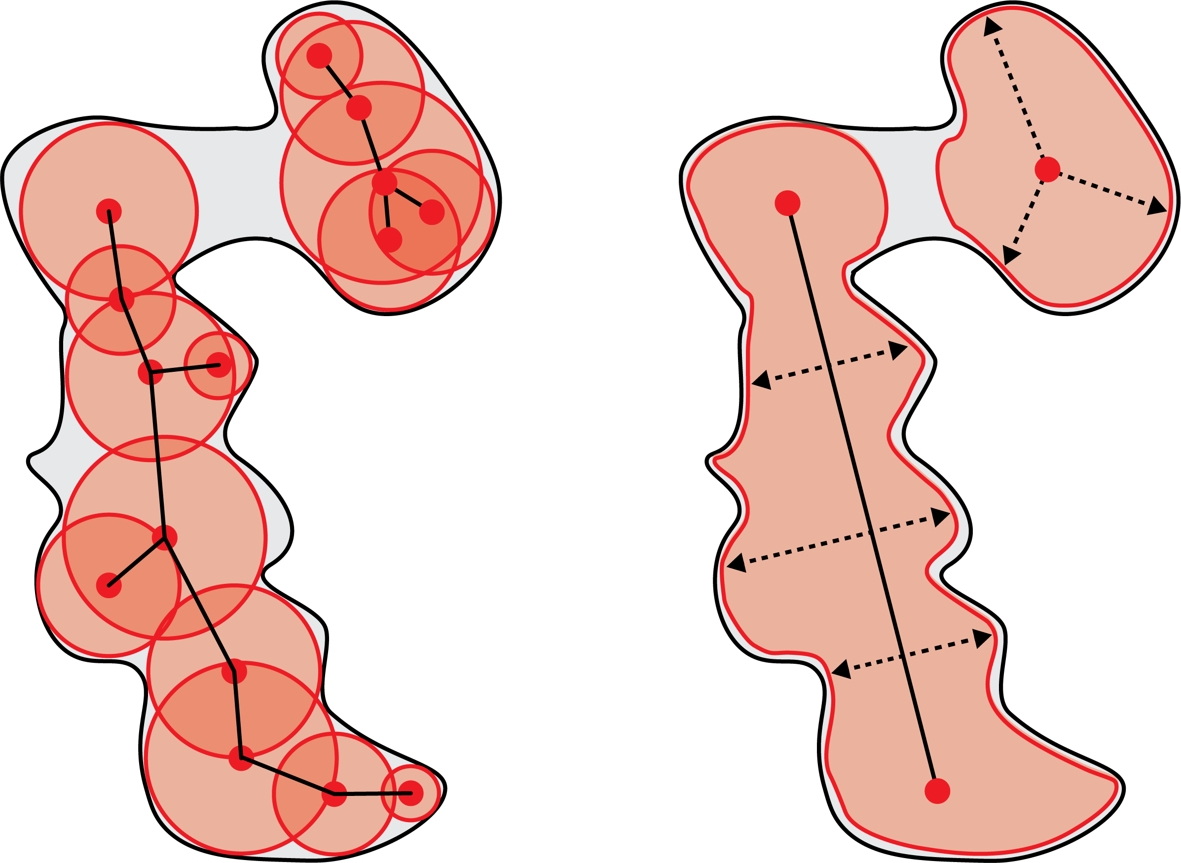
Figure 2. Generalized enveloping primitives in 2D. An illustration of employing our generalized enveloping primitives (right) for representing a 2D region. Compared to the standard medial primitives (left), our representation exhibits enhanced compactness when dealing with intricate, noisy, and high-curvature geometries.

4.1. Generalized Enveloping Primitives

We begin by outlining the formulation of generalized enveloping primitives. The basic idea is to replace the uniform, linearly interpolated primitives in the original medial axis with non-uniform, nonlinearly interpolated ones.

The generalized enveloping primitive is defined for all three types of medial mesh elements: $\mathbf{v}$, $\mathbf{e}$, and $\mathbf{f}$. For convenience, we define ${P}:=\mathrm{cvx}(\{v_{k}\}_{k=1}^{K})\in\{\mathbf{v},\mathbf{e},\mathbf{f}\}$, where $\mathrm{cvx}(\cdot)$ denotes the convex hull, $K\in\{1,2,3\}$ corresponds to the three types of medial mesh elements, respectively. We leverage the concept of $\epsilon$-neighborhood [Munkres, 2018] to define our generalized enveloping primitive.

Definition 4.1.

[Munkres, 2018, $\epsilon$-neighborhood] Let ${P}$ be a smooth submanifold in $\mathbb{R}^{3}$ and $\epsilon:{P}\mapsto\mathbb{R}^{+}$ be a smooth positive function. The $\epsilon$-neighborhood of ${P}$, denoted by ${P}^{\epsilon}$, is defined as,

(2) $${P}^{\epsilon}:=\big{\{}y\in\mathbb{R}^{3}\big{|}||y-x||_{2}<\epsilon(x)\ \text{for some}\ x\in{P}\big{\}}.$$

Furthermore, the $\epsilon$-neighborhood theorem asserts the existence of a surjective map between ${P}^{\epsilon}$ and ${P}$:

Theorem 4.2.

[Munkres, 2018, $\epsilon$-neighborhood theorem] For a smooth submanifold ${P}$ in $\mathbb{R}^{3}$, there exists a smooth positive function $\epsilon:{P}\mapsto\mathbb{R}^{+}$, such that (1) each $y\in{P}^{\epsilon}$ has a unique closest point $\pi_{\epsilon}(y)$ in ${P}$; (2) the map $\pi_{\epsilon}:{P}^{\epsilon}\mapsto{P}$ is a submersion. Moreover, if ${P}$ is compact, then $\epsilon$ can be taken to be a constant.

The $\epsilon$-neighborhood theorem ensures that for a medial mesh element ${P}$, there exists an appropriate constant ${\epsilon}$ to construct a smooth closed submanifold ${P}^{\epsilon}$ and establish a surjective map $\pi_{\epsilon}$ between ${P}^{\epsilon}$ and ${P}$. For more details of choosing ${\epsilon}$, we refer the readers to the proof of the theorem in  [Munkres, 2018]. If we consider the unit normal vector for each point $y$ on the boundary $\partial{P}^{\epsilon}$ of ${P}^{\epsilon}$, we obtain a submersion $g:N{\partial P}^{\epsilon}\mapsto{P}$,

$$g=\pi_{\epsilon}\circ f^{-1},$$

where $N{\partial P}^{\epsilon}=\{(y,n)|y\in\partial{P}^{\epsilon},n\in N_{p}\partial{P}^{\epsilon}\}$ denotes the unit normal bundle of ${\partial P}^{\epsilon}$, and $f:\partial{P}^{\epsilon}\mapsto N{\partial P}^{\epsilon}$, which is constructed from Gauss map of $\partial{P}^{\epsilon}$, maps between $\partial{P}^{\epsilon}$ and $N{\partial P}^{\epsilon}$. Here $f$ is bijective due to the fact that both ${P}^{\epsilon}$ and ${\partial P}^{\epsilon}$ are smooth and closed. The map $g$ serves as a crucial connector between the medial mesh element ${P}$ and the normal vectors of its $\epsilon$-neighborhood boundary $\partial{P}^{\epsilon}$. Essentially, $g$ associates each point in ${P}$ with a set of unit directional vectors – the normal vectors of $\partial{P}^{\epsilon}$, while the surjection of $\pi_{\epsilon}$ concurrently guarantees each such normal vector corresponds to a specific point in ${P}$. For any point $p\in{P}$, we denote its associated directional vectors as

(3) $$d_{p}({P}):=\big{\{}||n||_{2}=1\big{|}g(y,n)=p,\forall(y,n)\in N{\partial P}^{\epsilon}\big{\}},$$

and denote the set of all directional vectors of ${P}$ as

$$d({P})=\big{\{}d_{p}({P})|\forall p\in{P}\big{\}}.$$

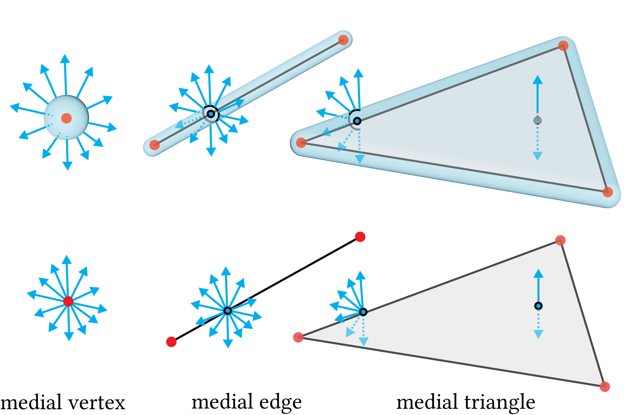
Figure 3. $\epsilon$-neighborhoods and corresponding normal bundles. Visualization of the boundary of ${P}^{\epsilon}$ for three medial mesh element types and the directional vectors $d({P})$ (only at selected points for clarity).

Fig. 3 shows $\partial{P}^{\epsilon}$ and $d({P})$ for all three types of medial mesh elements. In the case of a medial vertex, all the vectors in the set $d_{p}({P})$ belong to 2-sphere ${S}^{2}$. For a medial edge, the set of associated vectors $d_{p}({P})$ for any interior point $p$ forms a 1-sphere ${S}^{1}$. Meanwhile, at either endpoint of the edge, $d_{p}({P})$ forms a 2-hemisphere. For a medial triangle, the set $d_{p}({P})$ exhibits different characteristics for interior and boundary points. For each point located in the interior of the medial triangle, $d_{p}({P})$ consists of the normal vector of the triangle plane and its negative. For points in the interior of the three edges of the medial triangle, $d_{p}({P})$ comprises 1-hemisphere. For each of the three vertices at the corners of the medial triangle corners, $d_{p}({P})$ consists of a sphere wedge, whose angle is equal to the external angle of the triangle at the respective corner.

By leveraging the directional vectors $d_{p}({P})$, we have definition of a generalized enveloping primitive as follows:

Definition 4.3 (Generalized enveloping primitive).

Given a medial mesh element ${P}=\mathrm{cvx}(\{v_{k}\}_{k=1}^{K})$ and a smooth radius function $r(\cdot):d({P})\mapsto\mathbb{R}_{+}$, the generalized enveloping primitive is defined by an implicit function as

(4) $$\mathcal{E}_{{P}}(x)=||x-p_{x}||_{2}-r(d_{p_{x}}),d_{p_{x}}=(x-p_{x})/||x-p_{x}||_{2},$$

where $p_{x}=\mathrm{cp}(x;{P})$ is the point in ${P}$ which is closest to $x\in\mathbb{R}^{3}$.

We make $r(\cdot)$ to be smooth to comply with Theorem 4.2. One can observe that if $r(\cdot)\equiv\epsilon$, then the zero set of $\mathcal{E}_{{P}}(x)$ is $\partial{P}^{\epsilon}$. Fig. 2 and 4 illustrate the generalized enveloping primitives representing local regions of a 2D and a 3D shape, respectively. Compared to the ones used in the standard medial mesh, our generalized enveloping primitives can cover a diverse range of local regions using fewer primitives.

It is crucial to highlight that our generalized enveloping primitive formulation encompasses the standard enveloping primitives used in the medial axis as a special case, where the radius function $r(\cdot)$ is uniform and linearly interpolated (Fig. 5). More specifically, for a medial sphere,

$$r(d)\equiv\bar{r},\ \forall d\in d({P}).$$

For a medial cone ($K=2$) or a medial slab ($K=3$) with radii $\{\bar{r}_{k}\}_{k=1}^{K}$ at its corners, for each point $p\in{P}$,

$$r(d)\equiv\sum_{k=1}^{K}w_{k}(p)\bar{r}_{k},\ \forall d\in d_{p}({P}),$$

where $w_{k}(p)$ is the barycentric coordinates of $p$ on the medial element (edge or triangle).

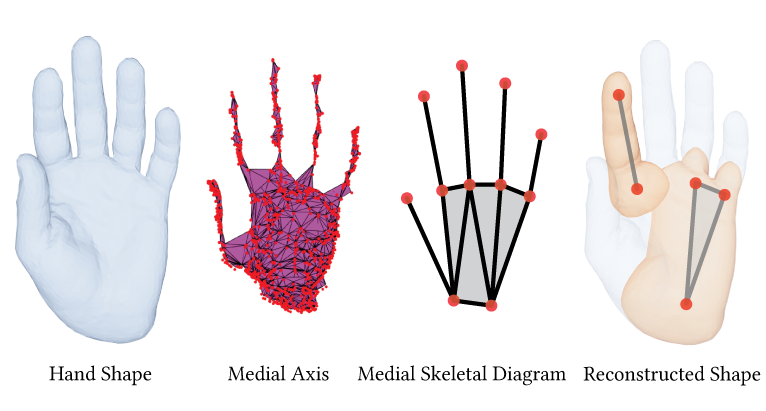
Figure 4. Medial skeletal diagram on Hand example. An illustration of employing our representation for a 3D hand shape. Compared to the medial axis, our medial skeletal diagram is more compact while maintaining the ability to accurately capture the detailed geometry. Our medial skeletal diagram offers a complete representation for 3D shapes.

4.2. Medial Skeletal Diagram

Our medial skeletal diagram (MSD) is constructed as a non-manifold triangular mesh with a much-reduced number of elements compared to the medial axis. Each element of this mesh is equipped with a generalized enveloping primitive. Formally,

Definition 4.4 (Medial skeletal diagram).

A medial skeletal diagram $\mathcal{D}$ is a non-manifold triangulated mesh $\mathcal{M}_{S}=(\mathsf{V},\mathsf{E},\mathsf{F})$ equipping with a generalized enveloping primitive $\mathcal{E}_{{P}}$ for each element ${P}\in\mathsf{V}\cup\mathsf{E}\cup\mathsf{F}$. $\mathcal{D}$ represents a 3D shape $\hat{\mathcal{S}}$ by $\hat{\mathcal{S}}=\bigcup_{{P}}\mathcal{E}_{{P}}$.

Medial skeletal diagram provides a compact skeleton of 3D shapes while maintaining the ability to accurately capture complex local regions and sharp features. As demonstrated in Fig. 4, under the same accuracy, the traditional medial axis requires 1,056 medial spheres and 2,449 medial slabs to represent the whole shape, resulting in a complex skeleton. By contrast, our method can efficiently and accurately cover the whole hand shape with 11 generalized medial spheres, 5 generalized medial cones, and 4 generalized medial slabs.

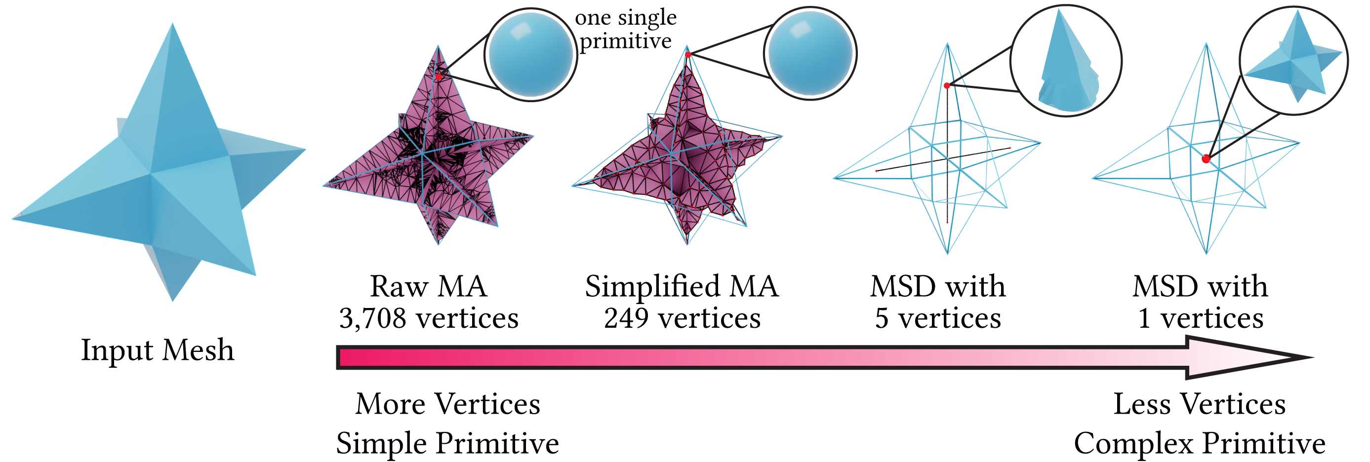
Figure 5. Generalization of our MSD. Our MSD spans a broad range of the skeleton representation spectrum. At one extreme lies the medial axis representation, characterized by simple primitives but intricate skeletons. At the opposite end, we have star-shaped regions that encompass just one, albeit complexly-shaped, primitive. The complexity of the MSD skeleton can be modulated by adjusting the fitting capability of each primitive.

Our medial skeletal diagram provides a complete representation for 3D shapes, incorporating the standard medial axis as a special case. It is capable of representing arbitrary 3D shapes (closed, oriented 2D manifolds, akin to the medial axis requirements).

Moreover, it pledges a more versatile representation compared to the standard approach. Under a worst-case scenario concerning the number of primitives needed, our method is not worse than the standard medial axis representation. This is because the upper limit of primitives necessary to fit the mesh in our model equals that in the medial axis, a correlation depicted in Fig. 5. In such instances, while the primitive remains simple, there is a trade-off in the form of an amplified skeletal complexity. Conversely, our diagram can encapsulate the entity with a single vertex for shapes representable through a solitary spherical function, such as the star domain demonstrated in Fig. 5.

Beyond this, our generalized enveloping primitives have several pivotal benefits:

• Providing a substantially simpler skeleton compared to conventional medial primitives, as demonstrated in Sec. 6.1. This compact skeletal structure is advantageous in various applications, highlighted in Sec. 6.2.

• Incorporating a well-researched and simple-to-build implicit function formulation, thereby becoming suitable for a range of tasks such as shape optimization [Chen et al., 2007], as further detailed in Sec. 6.2.1.

• Our primitives can be alternatively represented using orthogonal functions, including spherical/cylindrical harmonics [MacRobert, 1967; Smythe, 1988] and wavelets [Schröder and Sweldens, 1995], thereby reducing the mesh DOFs. In Sec. 6.2.5, we showcase a simple strategy to compress our generalized enveloping primitives.

5. Medial Skeletal Diagram Computation

To produce our medial skeletal diagram $\mathcal{D}$ for a given closed manifold triangular mesh $\mathcal{S}=(V_{\mathcal{S}},E_{\mathcal{S}},F_{\mathcal{S}})$, we begin with a target shape and its medial axis. Using an arbitrary set of points from the raw medial axis, we deterministically create the medial skeleton as detailed in Sec. 5.1. Subsequently, we fit our generalized enveloping primitives to each vertex, edge, and triangle of the skeleton to coincide with the target shape, as discussed in Sec. 5.2. The collective union of these primitives defines the final shape. This process forms an automated workflow to compute an MSD from any selection of vertices on the input medial axis.

Additionally, we introduce an efficient optimization pipeline to compute an optimal MSD. It aims to minimize the count of primitives while capturing the input shape in detail, preserving local geometry, tessellation, and vital topological nuances. Utilizing the aforementioned procedure, we employ a gradient-free optimizer to determine a vertex set ensuring the resultant 3D shape aligns with the input shape, as explained in Sec. 5.3. After optimization, the fitted primitives are refined through a feature-preserving refinement process considering both geometry and tessellation to achieve a precise match with the target mesh, as described in Sec. 5.4.

5.1. Medial Skeleton Construction

The idea behind constructing the medial skeleton $\mathcal{M}_{S}$ of a medial skeletal diagram $\mathcal{D}$ is to perform a “remeshing” of the medial axis by selecting a subset of vertices on the medial axis as constraints. Given that the medial axis is homotopy equivalent to the shape and the remeshing operation generally preserves topology, the resulting $\mathcal{M}_{S}$ can embody most of the topological information of the shape. We presume the input medial axis is high-quality and densely sampled. Meanwhile, by limiting the number of constrained vertices, we can maintain a compact number of discrete elements in $\mathcal{M}_{S}$.

There are primarily two ways for conducting vertex-constrained remeshing on the non-manifold raw medial mesh: 1) using mesh simplification operations, including vertex removal, edge collapse, and triangle collapse, while maintaining topology preservation through link conditions [Dey et al., 1999]; or 2) constructing a Voronoi diagram restricted to the raw medial mesh and using its dual, restricted Delaunay triangulation (RDT), for remeshing. Although mesh simplification operations can provide a strict guarantee of topology preservation, the remeshing result is affected by the order in which these operations are conducted. Conversely, the RDT method is order-independent but requires additional conditions to satisfy homotopy [Yan et al., 2009; Edelsbrunner and Shah, 1994; Amenta and Bern, 1998]. In our framework, we opt for the RDT approach, because the number of constrained vertices required to construct $\mathcal{M}_{S}$ is remarkably smaller than that in the raw medial axis. This means that a significant number of order-dependent operations would be required if the mesh simplification methods were used.

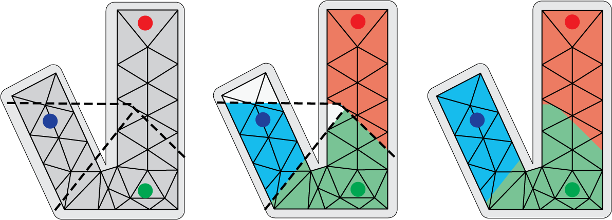
Figure 6. Illustration of RVC and its modification. The initial RVC (bounded by dash lines) may contain more than one connected component (CC) of the medial mesh $\mathcal{M}$. We assign each separate unassigned CC (white regions in the middle figure) to the nearest neighboring CC.

More specifically, given the target mesh $\mathcal{S}$ and its raw medial mesh $\mathcal{M}$, $\mathcal{M}_{S}$ construction algorithm takes a set of medial vertices $\mathsf{V}=\{\mathbf{v}\big{|}\mathbf{v}\in\mathcal{M}\}$ as input. These vertices can either be manually selected or obtained from the global optimization described in Sec. 5.3. The restricted Voronoi diagram $\mathrm{RVD}(\mathsf{V},\mathcal{M})$ is then constructed following Eq. (1). We split any element in $\mathcal{M}$ that intersects with a Voronoi face into two parts at the intersection and insert necessary vertices or edges to maintain it as a triangle mesh. Each vertex $\mathbf{v}$ corresponds to a restricted Voronoi cell $\mathrm{RVC}(\mathbf{v},\mathsf{V})$. Note that the $\mathrm{RVC}(\mathbf{v},\mathsf{V})$ might have more than one connected component (CC) of $\mathcal{M}$. Similar to [Xin et al., 2022], we modify each RVC to contain only one CC for the use of the following Delaunay triangulation. Specifically, we first perform a breadth-first search (BFS) rooted at $\mathbf{v}$ on $\mathcal{M}$ within each $\mathrm{RVC}(\mathbf{v},\mathsf{V})$. We then assign the CC expanded by BFS to $\mathbf{v}$. For those CCs not assigned to any vertices, i.e., they do not contain any vertex from the input set, we assign them to their nearest neighboring CC based on the distance between the RVC site and the center of the CC. Fig. 6 shows an example of the RVC modification. Since the raw medial mesh has only one CC for a closed shape, this assignment ensures that every element of $\mathcal{M}$ has an associated $\mathbf{v}$ and that each modified RVC is a single CC.

Then, the medial skeleton is obtained by RDT, which is dual to the RVD. Each $\mathbf{v}{\in}\mathsf{V}$ corresponds to a volumetric cell, i.e., the modified RVC. Each $\mathbf{e}{\in}\mathsf{E}$ connects two $\mathbf{v}$ if their corresponding modified RVCs share a common face of $\mathcal{M}$. Each $\mathbf{f}{\in}\mathsf{F}$ joins the vertices whose corresponding RVCs share a common edge of $\mathcal{M}$. We triangulate the polygonal surfaces of $\mathbf{f}$ to ensure $\mathsf{F}$ only consists of triangle faces. Note that RDT can yield volumetric objects when several RVC cells share a common vertex of $\mathcal{M}$. To address this, we adopt the thinning process described in [Wang et al., 2022a] to convert all tetrahedra in the RDT into two-dimensional sheets, thereby ensuring $\mathcal{M}_{S}$ does not contain any solid components.

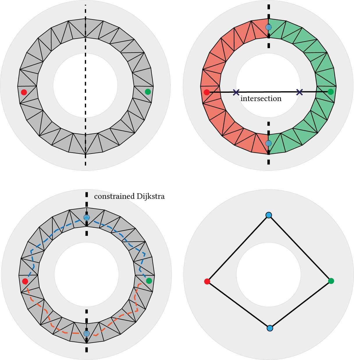
Figure 7. Revising RDT for a torus. The initial RVCs for two vertices of the torus exhibit two interfaces (bold dash lines), and the edge connecting these vertices intersects with the mesh (top right). We add additional vertices at each interface and compute the constrained shortest path (bottom left). The revised RDT (bottom right) remains entirely within the mesh and effectively captures the topology of the shape.

While the standard RDT approach successfully constructs the $\mathcal{M}_{S}$ for most shapes, there are two additional considerations needed, particularly for shapes of non-zero genus (example shown in Fig. 7): 1) neighboring RVCs can share more than one isolated interface (bold dash lines in Fig. 7); and 2) elements of the $\mathcal{M}_{S}$ might intersect with the target mesh $\mathcal{S}$, resulting in parts of the element being located outside the mesh.

To handle both situations, we first revise the edges of $\mathcal{M}_{S}$ and then update the associated RDT triangles. To address 1), we perform a BFS to identify all shared elements of $\mathcal{M}_{S}$ between every pair of neighboring RVCs, allowing us to locate their isolated interfaces. For each interface, we add a piecewise linear curve to $\mathcal{M}_{S}$ in $\mathcal{S}$ that originates from and terminates at the two vertices corresponding to the RVCs and passes through this interface. For situation 2), if an edge intersects with $\mathcal{S}$, we iteratively subdivide the edge until the tessellated edge is in $\mathcal{S}$. For each newly added point, we project it to the shortest path between these two endpoints on $\mathcal{M}$. Upon revising all the edges, we proceed to update the triangles incorporating any edges that have been revised in the previous two steps. Due to the addition of the edges, the triangles change to polygons. Therefore, we then perform triangulation of them. This approach effectively avoids triangle intersections with the target mesh for all the samples we tested in the paper. As an alternative, subdividing intersecting triangles and deforming them to fit inside the mesh could be explored in future work. Note that performing this revision results in a final medial element set for the medial skeletal diagram that may differ from the initial input set $\mathsf{V}$. We denote the final constructed medial skeleton as $\mathcal{M}_{S}=(\hat{\mathsf{V}},\hat{\mathsf{E}},\hat{\mathsf{F}})$, where $\mathsf{V}\subseteq\hat{\mathsf{V}}$.

5.2. Local Primitive Fitting

Primitive fitting involves discretizing the generalized enveloping primitive $\mathcal{E}_{{P}}$ in the space of the directions $d({P})$ for a given medial element $P$. This is achieved by the discretization of the $\epsilon$-neighborhood boundary $\partial P^{\epsilon}$, which provides a spatial tessellation for $\mathcal{E}_{{P}}$. A piecewise linear triangulated surface, denoted as $\mathcal{T}_{\partial P^{\epsilon}}=(V_{\epsilon},E_{{\epsilon}},F_{{\epsilon}})$, is used to discretize $\partial P^{\epsilon}$. For meshes scaled to the unit cube, we set $\epsilon=0.1$. This leads to the spatial discretization of directional vectors $d({P})$ aligning with the vertex normal vectors of $\mathcal{T}_{\partial P^{\epsilon}}$. We denote these unit discretized directional vectors as $\mathbf{d}\in\mathbb{R}^{|V_{\epsilon}|\times 3}$.

The discretized generalized enveloping primitive, denoted as $\mathcal{T}_{\mathcal{E}_{P}}=(V_{\mathcal{T}},E_{\mathcal{T}},F_{\mathcal{T}})$, is a triangle mesh derived by equipping $\mathcal{T}_{\partial P^{\epsilon}}$ with a discretized radius function $\mathbf{r}\in\mathbb{R}^{|V_{\epsilon}|}_{+}$. Each vertex of $\mathcal{T}_{\mathcal{E}_{P}}$ can only move along the direction $\mathbf{d}_{i}$, with distance indicated by $r_{i}$. Here, $E_{\mathcal{T}}=E_{{\epsilon}}$, $F_{\mathcal{T}}=F_{{\epsilon}}$, and $V_{\mathcal{T}}=\{v_{i}+{r}_{i}\mathbf{d}_{i},\forall v_{i}\in V_{\epsilon}\}$. Corresponding to the continuous case as in Def. 4.3, we use $\mathcal{E}(x;\mathcal{T}_{\mathcal{E}_{P}})$ to denote the implicit function of $\mathcal{T}_{\mathcal{E}_{P}}$ for any point $x\in\mathbb{R}^{3}$.

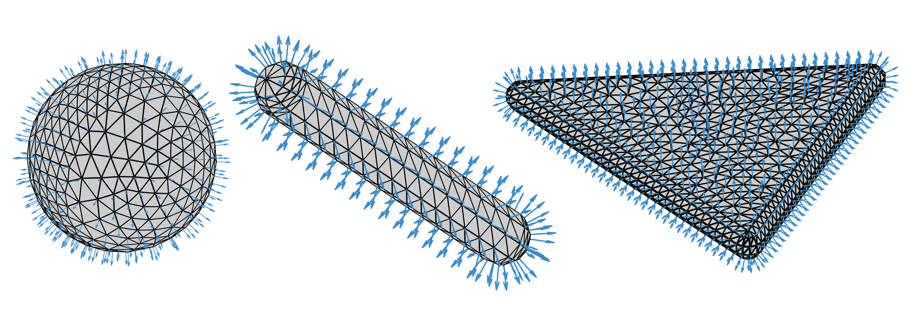
Figure 8. Discretized generalized enveloping primitives. We use triangle meshes to represent the discretized primitives. The directional vectors $d(P)$ become vertex normals (the blue vectors) in the discrete cases.

To be more specific, for the three types of medial elements, when we have a medial vertex $\mathbf{v}$, $\mathcal{T}_{\partial P^{\epsilon}}$ is represented by an isotropically meshed unit sphere centered at $\mathbf{v}$ with radius $\epsilon$. By modifying $\mathbf{r}$, each vertex of $\mathcal{T}_{\mathcal{E}_{P}}$ moves along the direction extending from the sphere center to the vertex itself. For a medial edge $\mathbf{e}$, we represent $\mathcal{T}_{\partial P^{\epsilon}}$ using two components: a uniformly meshed cylindrical wall and two end cap hemispheres. For a medial triangle $\mathbf{f}$, $\mathcal{T}_{\partial P^{\epsilon}}$ consists of three parts: two triangle planes, three half-cylindrical walls, and three spherical wedges. Fig. 8 illustrates the discretized mesh $\mathcal{T}_{\mathcal{E}_{P}}$ and the discretized directional vectors $\mathbf{d}$ for three cases. In general, the resolution of the primitive meshes is set such that it matches the input mesh resolution. For the generalized enveloping primitives of the medial vertices, we use a mesh with 1,588 vertices. For medial edges and triangles, the mesh resolution is determined by the size of the element. On average, the primitive mesh for an edge has 4,037 vertices and the mesh for a triangle has 1,360 vertices.

The goal of fitting primitive $\mathcal{T}_{\mathcal{E}_{P}}$ to the target mesh $\mathcal{S}$ is to find an optimal $\mathbf{r}^{*}$ such that $\mathbf{r}^{*}$ is smooth across $\mathcal{T}_{\mathcal{E}_{P}}$ and matches the local region of $\mathcal{S}$. The smoothness of the radius function is a prerequisite to upholding submersion in Thm. 4.2 and the requirement according to the definition of generalized enveloping primitive in Def. 4.3. Moreover, this smoothness prevents the occurrence of excessively large radii along certain directions, guaranteeing the locality of the primitives. We define the following energy optimization problem:

(5) $$\mathbf{r}^{*}=\operatorname*{arg\,min}_{\mathbf{r\in\mathbb{R}^{|V|}_{+}}} E_{\mathrm{smooth}}(\mathbf{r})+wE_{\mathrm{expansion}}(\mathbf{r})$$

$$\mathrm{s.t.} \mathbf{r}-\mathbf{r}^{\mathrm{max}}\leq\mathbf{0},$$

where the energies are defined as

(6) $$E_{\mathrm{smooth}}(\mathbf{r})=\mathbf{r}^{\intercal}\mathbf{L}^{\intercal}\mathbf{L}\mathbf{r},\ \ E_{\mathrm{expansion}}(\mathbf{r})=||\mathbf{r}-\mathbf{r}^{\mathrm{tgt}}||_{2}^{2}.$$

In the optimization problem, $E_{\mathrm{smooth}}$ penalizes non-smoothness of the radii across $\mathcal{T}_{\mathcal{E}_{P}}$. We choose $\mathbf{L}$ to be the graph Laplacian matrix of the initial $\mathcal{T}_{\mathcal{E}_{P}}$. $\textbf{r}^{\mathrm{tgt}}$ determines how much the primitives grow. $E_{\mathrm{expansion}}$ aims to expand $\mathcal{T}_{\mathcal{E}_{P}}$ and increase the radii $\mathbf{r}$ to a larger target value $\mathbf{r}^{\mathrm{tgt}}$, while the constraint prevents the penetration of $\mathcal{T}_{\mathcal{E}_{P}}$ into the target mesh $\mathcal{S}$. $\mathbf{r}^{\mathrm{max}}\in\mathbb{R}^{|V|}_{+}$ is the maximal expansion radii of all directions. This is precomputed by measuring the distance from $v_{i}$ to the first intersection point between the target mesh $\mathcal{S}$ and the ray that originates at $v_{i}$ with directional vector $\mathbf{d}_{i}$. In Fig. 9, we show how weight $w$ balances the trade-off between the expansion and the mitigation of exceedingly long radii. In our implementation, we choose $w=10$ consistently for all the examples.

Figure 9. Effect of $w$ in local primitive fitting. The weight $w$ balances the trade-off between expansion and smoothness. An overly large $w$ can induce excessively long radii, especially in tubular shapes, while a notably small $w$ may over-smooth the primitive, failing to capture necessary geometry details (bottom row). As a result, a more smoothed primitive requires more skeleton elements, and vice versa (top row). We choose $w=10$ in our implementation.

Eq. (5) is a quadratic programming problem that can be solved using standard techniques, such as the interior point method. To improve performance, we employ an alternating optimization approach inspired by [Bouaziz et al., 2014] instead of a Newton-type solver. For each iteration, we first identify the index set $\mathcal{Z}$ which includes all directions having a radius larger than $\mathbf{r}_{i}^{\mathrm{max}}$. Then, we optimize the following modified objective:

(7) $$\tilde{\mathbf{r}}^{(t)}=\operatorname*{arg\,min}_{\mathbf{r}}\ E_{\mathrm{smooth}}(\mathbf{r})+wE_{\mathrm{expansion}}(\mathbf{r})+\sum_{i\in\mathcal{Z}}\Delta{{}^{(t)}}(r_{i}),$$

(8) $$\Delta^{(t)}(r_{i})=\hat{w}||r_{i}-r_{i}^{\mathrm{max}}||_{2}^{2},$$

where $\hat{w}$ is a constant ($\hat{w}=10^{4}$) for the contact constraints. We execute up to 15 iterations; however, our solver typically converges in fewer than 5 iterations, with an average fitting time of 0.08 seconds per primitive. Compared to Newton-type optimization methods, the objective is quadratic and can be minimized with a single linear solver, thereby speeding up the optimization process. Our optimization approach also benefits from the use of generalized enveloping primitives. Compared to the commonly used vertex positions, the radii $\mathbf{r}$ has a much-reduced number of degrees of freedom (DOF) as the optimization variable and simplifies the handling of contact constraints.

In our implementation, the initial radii of enveloping elements are computed based on the closest distance from the shape to their centers. To increase the robustness of primitive expansion, we progressively increase $\textbf{r}^{\mathrm{tgt}}$ by $10\%$ of the initial radius for each ray direction and solve Eq. (5) at each progression. $\mathbf{r}^{\mathrm{tgt}}$ is increased $25$ times in our experiments.

5.3. Global Optimization

Figure 10. Effect of each energy term. (a) Without any regularization, the skeleton vertices are unevenly distributed along the input medial axis. (b) Incorporating $E_{\mathrm{centrality}}$ addresses this issue. (c) Furthermore, introducing $E_{\mathrm{count}}$ reduces the vertex count (from 9 vertices to 8 vertices), leading to a simpler skeleton.

Figure 11. Intermediate results and energy convergence curves of the global optimization. The global optimization is framed to obtain an optimal medial skeletal diagram that strives to maximize target mesh coverage while minimizing the number of primitives used. A gradient-free optimization method is carried out to efficiently optimize the energies. During the optimization, we incrementally add new points to each isolated uncovered volume and fit primitives (shown in the orange color). The geometric details such as dragon horns, tails, and claws are successfully captured, as highlighted by the rectangles. Note that energy spikes are encountered due to the introduction of new trial points by the NM optimizer, as it does not ensure a consistent decrease in energy.

In the previous sections, we discussed how the construction of the medial skeletal diagram $\mathcal{D}$ for a given target mesh is determined by the input set of candidate vertices. We use vector $\mathbf{V}\in\mathbb{R}^{|\mathsf{V}|\times 3}$ to indicate the input candidate vertices and denote the resulting medial skeletal diagram by $\mathcal{D}(\mathbf{V})=(\mathcal{M}_{S}(\mathbf{V}),\{\mathcal{T}_{\mathcal{E}_{P}}\}_{P\in\mathcal{M}_{S}(\mathbf{V})})$. We now present a global optimization scheme that aims to obtain an optimal $\mathcal{D}(V^{*})$ that strives to maximize target mesh coverage while minimizing the number of primitives used. The global optimization is formulated as follows:

(9) $$\mathbf{V}^{*}=\operatorname*{arg\,min}_{\mathbf{V}\in\mathcal{M}}\ E_{\mathrm{coverage}}(\mathcal{D}(\mathbf{V}))+c_{1}E_{\mathrm{centrality}}(\mathbf{V})+c_{2}E_{\mathrm{count}}(\mathbf{V}),$$

where each energy term is defined as,

$$E_{\mathrm{coverage}}(\mathcal{D}(\mathbf{V})) =\sum_{v\in V_{\mathcal{S}}}\begin{cases}-A(v)&\text{if }\exists P\in\mathcal{M}_{S}(\mathbf{V}),\ \text{s.t. }\mathcal{E}(v;\mathcal{T}_{\mathcal{E}_{P}})<\delta\\ 0&\text{o.w.}\end{cases},$$

$$E_{\mathrm{centrality}}(\mathbf{V}) =\sum_{\mathbf{v}\in\mathbf{V}}||\mathbf{v}-c(\mathrm{RVC}(\mathbf{v},\mathbf{V}))||_{2}^{2},$$

$$E_{\mathrm{count}}(\mathbf{V}) =||\mathbf{V}|-|\hat{\mathbf{V}}||.$$

Here, $A(v)$ represents the normalized vertex area of $v$ with respect to the total surface area of $\mathcal{S}$, $P\in\hat{\mathsf{V}}\cup\hat{\mathsf{E}}\cup\hat{\mathsf{F}}$ is the primitive, and $c(\cdot)$ denotes the centroid of the restricted Voronoi cell.

Input: medial axis $\mathcal{M}$, target shape $\mathcal{S}$, and set of vertices $\mathbf{\bar{V}}$

Output: energy value $E$

$\mathbf{V}\leftarrow$ $\mathbf{\bar{V}}$ projection onto $\mathcal{M}$

Construct the medial skeleton $\mathcal{M}_{S}(\mathbf{V})$ (Sec. 5.1)

Fit primitives $\{\mathcal{T}_{\mathcal{E}_{P}}\}_{P\in\mathcal{M}_{S}(\mathbf{V})}$ to $\mathcal{S}$ (Sec. 5.2)

$E\leftarrow$ $E_{\textrm{coverage}}(\mathcal{D}(\mathbf{V}))+c_{1}E_{\mathrm{centrality}}(\mathbf{V})+c_{2}E_{\mathrm{count}}(\mathbf{V})$

return $E$

Algorithm 1 Compute Energy

The objective in Eq. (9) consists of three energy terms. $E_{\mathrm{coverage}}(\cdot)$ measures the target mesh coverage of $\mathcal{D}$. This energy is calculated by enumerating all the vertices of the target mesh $\mathcal{S}$; if a vertex $v$ is located within a small distance $\delta$ from any fitted primitive, it is then considered to be covered by $\mathcal{D}$, and its vertex area contributes negatively to the energy value. $E_{\mathrm{centrality}}(\cdot)$ enforces the uniformity in the distribution of RVCs within the space. This is inspired by Lloyd’s algorithm for Voronoi relaxation [Lloyd, 1982], which aims to achieve uniformly sized Voronoi cells by iteratively moving each input point toward the center of its corresponding Voronoi cell. In our context, we strive for a uniformly distributed medial skeletal diagram by penalizing the distance between the input selected point and the corresponding RVC centroid. $E_{\mathrm{count}}(\cdot)$ imposes a penalty for the additional vertices introduced during the construction of the medial skeletal diagram, aiming to minimize the complexity of the resulting structure. In Fig. 10, we show that each term plays an important role in regularizing the objective. Given the non-differentiability of the objective, we use the Nelder-Mead (NM) simplex algorithm [Richardson and Kuester, 1973], a gradient-free optimization method, to optimize Eq. (9).

To initiate the optimization, we begin with a set of initial candidate vertices $\mathbf{V}^{(0)}$ selected from the medial axis $\mathcal{M}$. The selection is performed by maximizing the shortest-path distance on the $\mathcal{M}$ between each pair of samples. Then, we use NM simplex algorithm to optimize objective (9) evaluated by Alg. 1. At the beginning of each iteration, we project the input vertex positions onto $\mathcal{M}$ for constructing the medial skeleton. The iteration proceeds until 1) the objective (9) no longer decreases for a consecutive of five iterations; 2) the primitives fully cover the target mesh; or 3) the maximal number of iterations is reached.

To speed up the optimization, we incrementally optimize $\mathbf{V}^{*}$. We configure the initial set $\mathbf{V}^{(0)}$ to be small, which can be as few as one vertex ($|\mathbf{V}^{(0)}|=1$). We then optimize Eq. (9) for $t$ iterations, yielding the result $\tilde{\mathbf{V}}^{(t)}$. For every $t$ iteration, we check if there are individual regions remaining uncovered. If that is the case, we add a candidate vertex at the volume center for the first $n$ largest regions. The newly added vertices $\mathbf{V}_{\mathrm{new}}^{(t)}$ combined with the existing candidate vertices form the final candidate set $\mathbf{V}^{(t+1)}=[\tilde{\mathbf{V}}^{(t)};\mathbf{V}_{\mathrm{new}}^{(t)}]$. The iteration proceeds until the stopping criteria are met. We only optimize $\mathbf{V}_{\mathrm{new}}^{(t)}$ while freezing the optimized $\tilde{\mathbf{V}}^{(t)}$ for performance consideration. In our implementation, we set $c_{1}=1$ and $c_{2}=10^{-3}$ consistently for all the examples. Fig. 11 shows the intermediate results and energy convergence curves for three examples.

5.4. Feature-Preserving Refinement

Our optimization pipeline produces a medial skeletal diagram with maximal coverage of the target mesh. As we discretize the generalized enveloping primitives to a triangle mesh, however, despite the radii of primitive mesh vertices might align with the target mesh, the triangle faces of the primitive mesh could still significantly deviate from the target mesh due to the differences in tessellations of the primitive mesh and the target mesh. To address this, we propose a robustness refinement process that allows our representation to “exactly” match the target mesh in terms of geometry and “almost exactly” mirror its tessellation. By “almost exactly”, we indicate that the tessellation of the target mesh is entirely encompassed within the refined primitive. Moreover, our refinement method produces consistency post-refinement primitives which satisfy the definition of generalized enveloping primitive, retaining the advantages of these primitives as discussed in Sec. 4.1. Guaranteeing consistency filters out many trivial refinement methods. For instance, simply dilating the primitive and boolean-intersecting with the target mesh may violate the consistency, as the resulting primitive may exhibit multiple radius values along one single direction for a profoundly concave shape.

The core strategy is to refine each fitted generalized enveloping primitive mesh so that both its radius function and tessellation in the regions that are close to the target mesh are precisely matched with the target mesh. To achieve both consistency and robustness, our refinement process consists of four steps, as shown in Fig 12. For each fitted generalized enveloping primitive $\mathcal{T}_{\mathcal{E}_{P}}$, 1) we initially identify the sub-surface of the target mesh that resides within a $\delta$ distance to $\mathcal{T}_{\mathcal{E}_{P}}$ and project its tessellation onto $\mathcal{T}_{\mathcal{E}_{P}}$. This step ensures that the tessellation of the sub-surface, including vertices, edges, and triangles, is fully encompassed within $\mathcal{T}_{\mathcal{E}_{P}}$. 2) We then remove redundant edges that do not contribute to any geometric and tessellation features of the target mesh. 3) Next, we update the vertices positions of $\mathcal{{T}}_{\mathcal{E}_{P}}$ such that the geometry of the sub-surface exactly aligns with the target mesh. Because the primitive mesh encompasses the tessellation of the target mesh, updating the vertex position makes the primitive mesh match the target mesh exactly in the selected sub-surface. 4) We finally carry out a mesh clean-up by removing small edges and triangles without affecting the matched geometry and tessellation. We implement the above four steps using exact rational arithmetic to ensure the robustness of our process. For more detailed information on the implementation, we direct readers to consult the supplementary materials. In Fig. 13, we show three example primitives undergoing the refinement process.

Figure 12. The procedure of our feature-preserving refinement. The process consists of four steps. In the first step, we refine the primitive mesh such that it contains the tessellation of the target mesh (step 1). Next, we remove redundant edges in each triangle surface patch and produce a triangulated primitive mesh (step 2). Then, the vertex positions are updated based on their primitive type (step 3). Finally, we clean up the small triangles and edges as much as possible while preserving the target mesh tessellation (step 4). Here for 2D illustration, we omit step 3 and refer the readers to Fig. 13 for a 3D example.

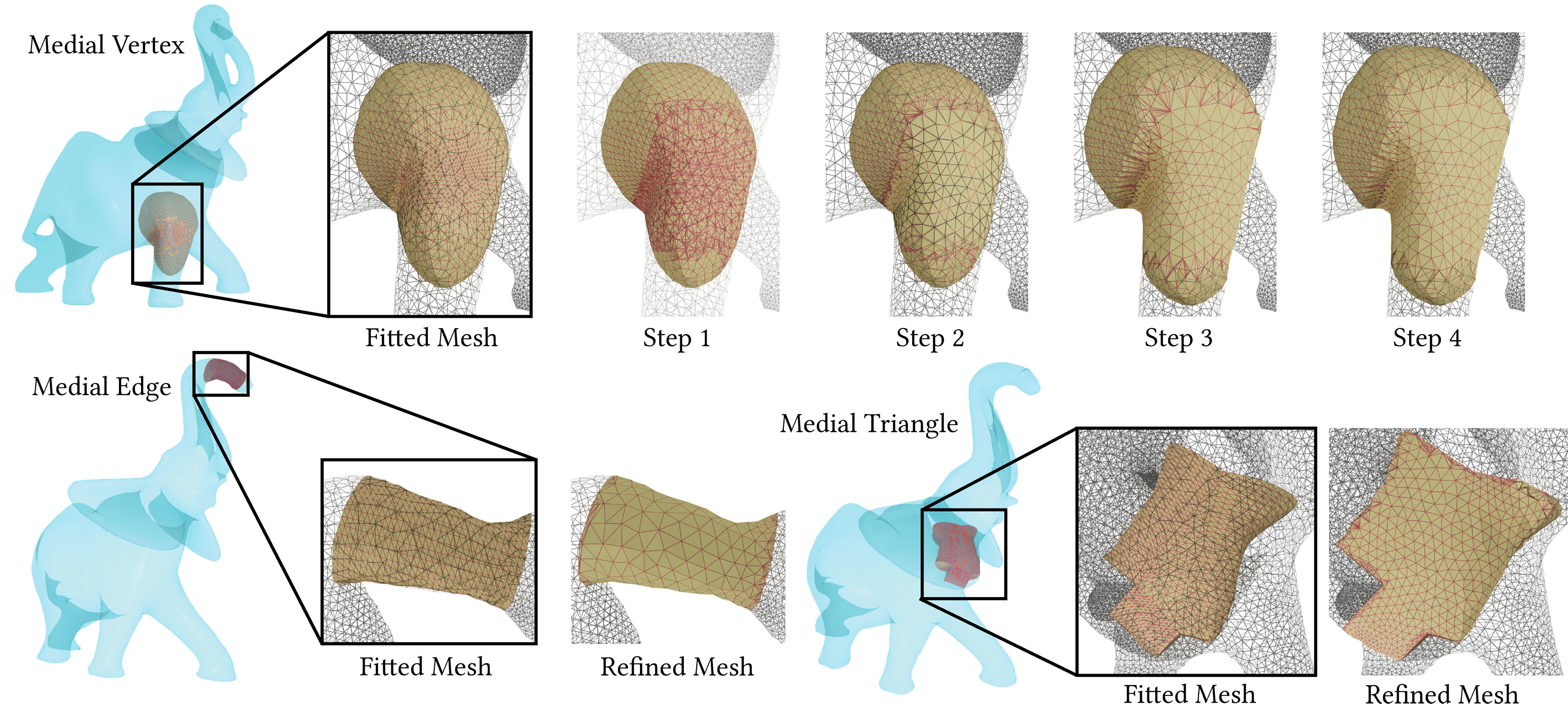
Figure 13. Results of our feature-preserving refinement on primitive meshes of all three types. In the first row, we show the step-by-step intermediate results obtained during the process of refining a medial vertex primitive mesh. The primitive mesh undergoes refinement aligning with the target mesh in terms of both geometry and tessellation. The second row offers additional examples featuring the refinement process for the medial edge primitive mesh and medial triangle primitive mesh.

6. Experiments

Our experiments are run on a desktop with an AMD Ryzen 9 5950X 16-core CPU and 64GB RAM. We use GMP, MPFR, and CGAL for low-level arithmetic and geometric kernels. To demonstrate the effectiveness and robustness of our method, we evaluate our algorithm on $100$ closed manifold triangle meshes. They are sourced from V-HACD dataset [Mamou, 2016], AIM@Shape Repository [Cohen-Steiner and Morvan, 2003], and the McGill 3D shape benchmark [Fang et al., 2008]. The size of all shapes is normalized to the $[0,1]$ range. For all shapes in our benchmark, we apply the same set of parameters to the local fitting (mentioned in Sec. 5.2), For the global optimization, we set the initial number of candidate vertices $|\mathbf{V}^{0}|=10$. After the first $50$ iterations, we add either three new vertices or five new vertices every $30$ iterations ($n=3$ or $n=5$), depending on which one gives the better result. The coefficient for each energy term is mentioned in Sec. 5.3. All the experimental results are conducted using a consistent parameter setting. We choose to use the simplified medial axis obtained from [Dou et al., 2022] as the initial start of medial skeletal diagram construction to strike a balance between computational speed and skeleton accuracy. Note that our approach is not strictly tied to this choice, but can readily accommodate other variants of medial axis representations as inputs. Statistics of the computational cost required to construct our representation are shown in Fig. 14 and Table 1.

Table 1. Average Timing for global optimization and refinement.

Per Iter.	Projection	0.006s
	MSD Construction	4.12s
	Primitive Fitting	4.64s
	Energy Evaluation	2.71s
	Total Global Opt.	11.57s
	Total Global Opt. #iter.	51
	Refinement	10.78s

Baselines.

We include six baselines: (1) MAT [Amenta and Bern, 1998], the raw medial axis transformation; (2) MATFP [Wang et al., 2022a], a state-of-the-art technique for computing the MAT while preserving features; (3) LS Skeleton [Bærentzen and Rotenberg, 2021], a curve skeletonization approach grounded in local separators; (4) Coverage Axis (CA) [Dou et al., 2022], a shape skeletonization method that simplifies from MAT; (5) Point2Skeleton (P2S) [Lin et al., 2021], a deep learning-based method for constructing medial meshes from point clouds; (6) CoACD (ACD) [Wei et al., 2022], a state-of-the-art method for convex decomposition.

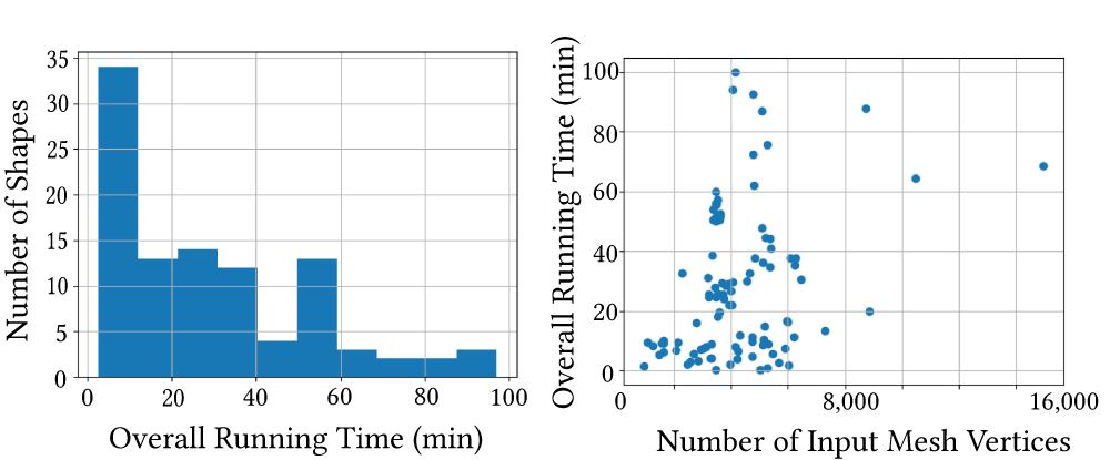
Figure 14. Statistics of the computational cost for constructing medial skeletal diagram from an input shape, including a histogram of overall running time across the $100$ shape benchmark and the complexity of input mesh v.s. running time. The computational time is principally influenced by the input mesh size (impacting feature-preserving refinement) and the shape complexity (impacting global optimization).

Metrics.

Following [Wang et al., 2022a; Dou et al., 2022; Lin et al., 2021], we use the two-sided average vertex-to-surface distance error, denoted as $\bar{\epsilon}$, to evaluate the surface reconstruction accuracy using medial meshes. $\bar{\epsilon}^{1}$ is the one-sided average vertex-to-surface distance from the original surface to the reconstructed surface and $\bar{\epsilon}^{2}$ is the distance in the reverse direction. We also report the number of medial elements, including the vertices $\#v$, edges $\#e$, and triangles $\#f$, to compare the compactness of discrete elements in different representations. To offer a more complete overview, we detail the number of continuous parameters ($\#$c) associated with different representations. For baseline methods, we report $\#$c as the total degree of freedom of medial spheres (the count of medial vertices in the skeleton times four). For our method, we report the total number of directional vectors for all primitives plus the total degree of freedom of medial vertices. To ensure a fair comparison of reconstruction error, in the case of MAT, we increase the target mesh resolution without changing its geometry to obtain a skeleton that has a comparable magnitude of $\#$c to that of our method. For MATFP, LS, CA, and P2S, following their original papers, we reconstruct the mesh from the skeleton using medial spheres, cones, and slabs. In the case of ACD, where there is no reconstruction involved, we only report the number of decomposed domains (represented by $\#v$) and $\#e$ for every pair of adjacent domains. The number of unique edges $\#e$ of MATFP and the number of faces $\#f$ of LS Skeleton are omitted from the table as these counts are zero across all shapes. We consider an edge unique if it is not a triangle edge in MATFP. Since LS only produces curve skeletons, it does not contain any triangles.

Table 2. Quantitative comparisons on the number of discrete and continuous parameters in the representation and shape reconstruction error on the benchmark of $\mathbf{100}$ shapes. We count the number of vertices ($\#v$), the number of edges ($\#e$), the number of triangles ($\#f$), and the sum of them (#d) for discrete elements. In addition, we provide the number of continuous parameters in row #c. For the reconstruction errors, $\bar{\epsilon}^{1}$ is the one-sided average vertex-to-surface distance from the original surface to the reconstructed surface, $\bar{\epsilon}^{2}$ is the distance in the reverse direction. $\bar{\epsilon}$ is the two-sided average vertex-to-surface distance error. We compare our method with six existing methods: MAT, MATFP (MFP), CoACD (ACD), LS Skeleton (LS), Point2Skeleton (P2S), and Coverage Axis (CA). Our medial skeletal diagram demonstrates superior compactness on discrete elements and the highest reconstruction accuracy compared to other representations.

		MAT	MFP	ACD	LS	P2S	CA	Ours
$\#v$	Min	17,955	692	3	4	100	57	3
	Max	37,705	4,119	192	195	100	738	277
	Avg	32,539	2,110	27	57	100	229	26
$\#e$	Min	0	–	2	3	0	0	0
	Max	144	–	639	192	35	131	81
	Avg	15	–	57	57	3	18	9
$\#f$	Min	31,042	1,445	–	–	136	0	0
	Max	82,297	10,232	–	–	346	1,437	457
	Avg	63,279	4,835	–	–	233	385	24
$\#$d	Avg	95,833	6,945	84	114	337	632	58
$\#$c	Min	71,820	2,768	–	16	400	228	4,594
	Max	150,820	16,476	–	780	400	2,952	497,770
	Avg	130,154	8,440	4,423	229	400	918	94,168
$\bar{\epsilon}^{1}$	Min	0.06	0.044	–	0.59	0.76	0.17	0
	Max	3.09	3.18	–	24.34	2.92	12.37	0.41
	Avg	0.31	0.31	–	4.42	1.31	0.54	0.029
$\bar{\epsilon}^{2}$	Min	0.11	0.029	–	0.39	1.14	0.14	0
	Max	0.48	0.68	–	10.03	10.35	0.83	0.098
	Avg	0.24	0.15	–	2.54	2.22	0.34	0.008
$\bar{\epsilon}$	Avg	0.40 ($+129\%$)	0.31	–	4.43 ($+1324\%$)	2.22 ($+615\%)$	0.54 ($+74\%$)	0.031 ($\mathbf{-90\%}$)

6.1. Comparisons and Discussions

The quantitative comparisons between our method and the baselines, conducted on the $100$ meshes, are presented in Table 2. Our method uses the fewest skeletal elements and achieves the lowest two-sided mean distance error relative to all other methods examined. Despite the increased number of continuous parameters in our representation, as detailed in subsequent sections (Sec. 6.2.1 and 6.2.5), this does not introduce complications but rather aids in finding a better solution. Our mean reconstruction error is 10% of MATFP and 7.8% of MAT, the two methods yielding the least reconstruction error among all baselines. While MATFP employs 91.0% fewer continuous parameters with reconstruction errors that are 10 times greater compared to our method, increasing the number of MATFP’s continuous parameters to roughly match those of our method–by densely sampling the input mesh–only reduces its reconstruction errors by 60%. which is still 6 times higher than that of our approach. On the other hand, despite that MAT uses more continuous parameters, it fails to seamlessly align with the target mesh given a finite number of medial primitives.

To demonstrate the effectiveness of our feature-preserving refinement, we also measure the two-sided mean distance error of the fitting-only results. Among $100$ shapes, our fitting-only reconstruction reports $0.22$ error, $7\times$ larger than the error after the refinement post-processing. Nonetheless, it is still smaller than the errors of all existing methods. Furthermore, we also measure the two-sided Hausdorff distance between the input shape and the reconstructed shape. Our representation reports $1.81$ on average over $100$ shapes, lower than the mean distance error of both LS and P2S. Moreover, ours is also lower than the two-sided Hausdorff distance of both CA and MATFP, which are $3.64$ and $2.22$, respectively. In addition to quantitative comparisons, we also show a set of qualitative results on various shapes from these $100$ meshes in Fig. 15 and 16. Compared with other baselines, our representation produces visually simpler skeletons and more accurate reconstruction.

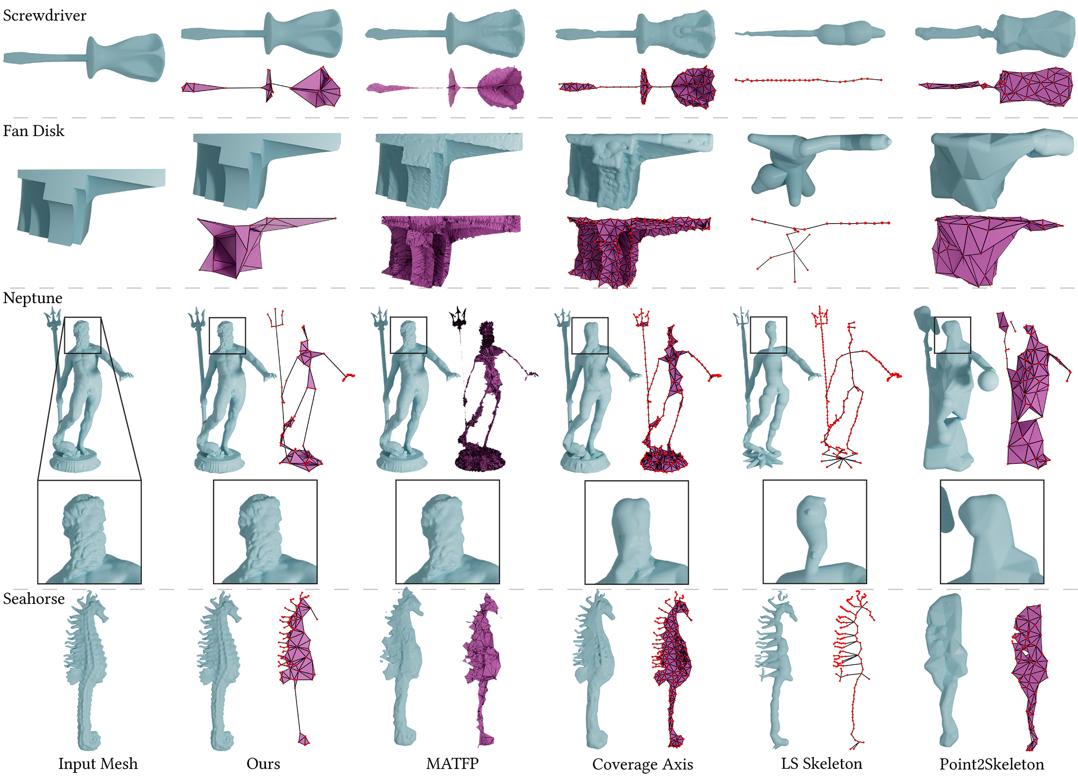
Figure 15. Qualitative comparison of the skeletal representation and reconstructed mesh (part 1/2), involving four baseline methods and our proposed method. We omit the visualization of medial vertices for MATFP due to their excessive quantity.

Comparison with Medial Axis Transform

We compare our method with MATFP [Wang et al., 2022a] in the context of the quality of the reconstructed mesh. MATFP is highly regarded for its remarkable precision and is tailored to preserve external features such as sharp edges and corners of the input mesh surface. This algorithm is essentially a superior variant of the medial axis transforms. MATFP requires two input thresholds for controlling sharp feature detection. We use the default parameters provided within the official source code for all $100$ shapes. Our method demonstrates a better performance with MATFP regarding reconstruction accuracy. This is attributed to our refinement process which exactly matches the geometry and tessellation of the reconstructed shape from our method with the input mesh – a feature that is notably missing in existing medial axis representations including MATFP. What truly distinguishes our method is its ability to achieve these results using significantly fewer medial elements. This simplicity is largely due to our utilization of generalized enveloping primitives. Thus, while maintaining a high level of accuracy akin to MATFP, our method outperforms it in terms of the skeleton simplicity, with a reduction in the number of medial elements by two orders of magnitude.

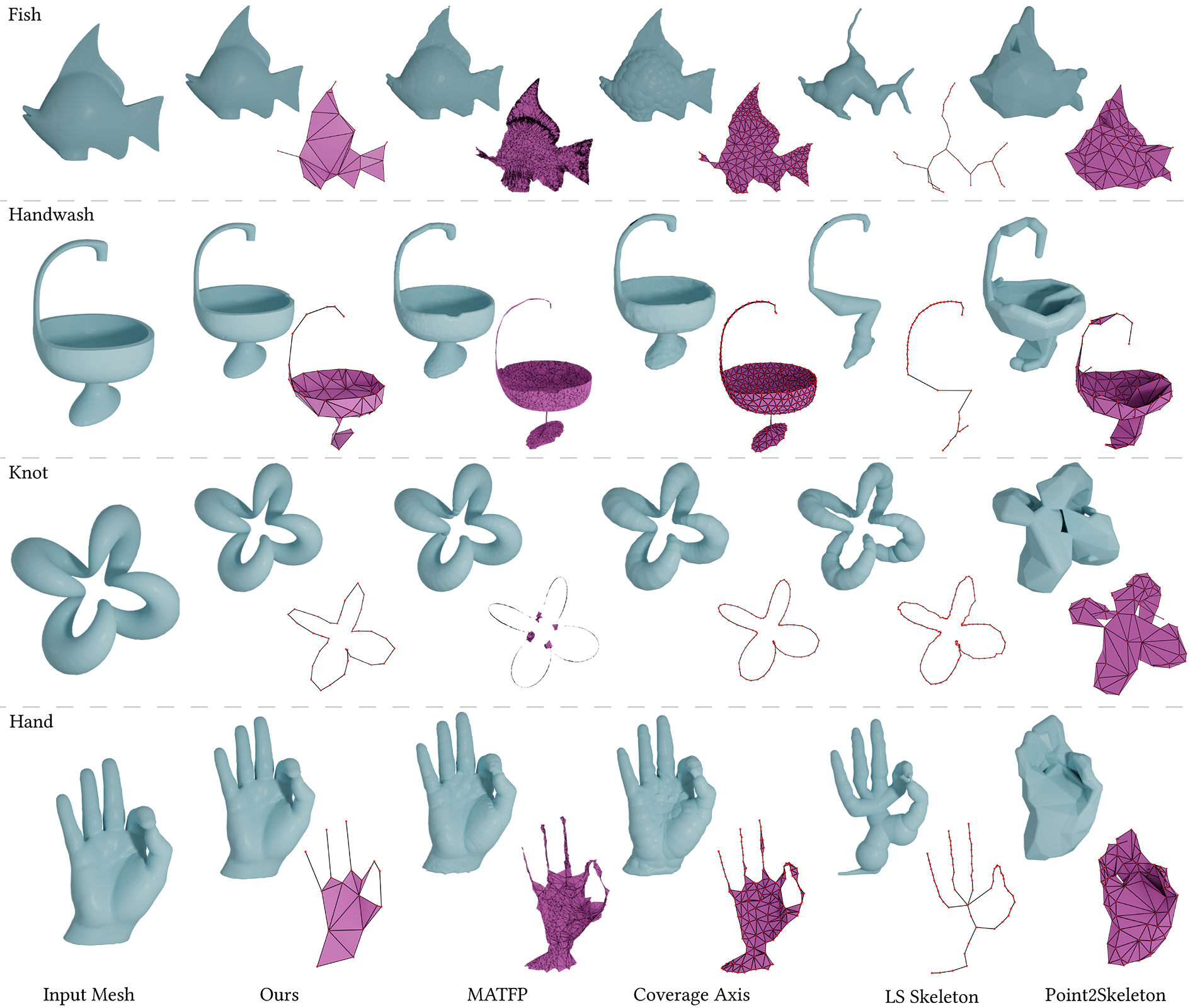
Figure 16. Qualitative comparison of the skeletal representation and reconstructed mesh (part 2/2), involving four baseline methods and our proposed method. We omit the visualization of medial vertices for MATFP due to their excessive quantity.

Comparison with Simplified Skeleton-based Methods

We consider two simplified skeleton-based methods: Coverage Axis [Dou et al., 2022] and Point2Skeleton [Lin et al., 2021]. Both methodologies are based on a similar process that simplifies the raw medial axis to preserve the geometric and topological features of the input mesh surface. Coverage Axis employs Mixed Integer Linear Programming (MILP) to minimize the count of medial vertices while ensuring comprehensive coverage of all the input mesh surface points. This tactic results in superior reconstruction accuracy when compared to other baseline methods, owing to its explicit optimization for this particular objective. On the other hand, Point2Skeleton adopts a data-driven strategy, leveraging deep neural networks to predict skeletal points and their interconnections. As it is a data-driven method, however, it does not generalize to arbitrary input shapes. The output of a neural network necessitates a fixed number of vertices ($100$ in the official implementation), which can pose challenges when generalizing to unseen shapes that deviate from the training dataset. Both simplified skeleton methods rely on spheres, cones, and slabs for surface reconstruction. The primary objective of these methods is to optimize point coverage, so inadvertently introduce errors in the surface reconstruction process. This stems from the nature of these primitives - their geometric shapes are fixed and lack the flexibility to adapt to arbitrary regions, which can result in an inaccurate approximation of the original mesh surface. By contrast, our approach leverages the mesh representation of generalized primitives and benefits from the refinement technique. Neptune and Seahorse in Fig. 15 are two evident examples.

Comparison with Curve Skeletons

LS Skeleton [Bærentzen and Rotenberg, 2021] is a state-of-the-art method for curve skeletonization. Notable for its simplicity and smoothness in representing shapes, LS Skeleton shares a common drawback with other curve skeleton-based methods: it struggles to accurately represent large flat regions present in the input shape. This is particularly problematic for CAD models that frequently feature such flat regions. Screwdriver and Fan disk example in Fig. 15 provide evidence. In this case, a noticeable advantage of our approach is its ability to represent an entire rectangular region with a few triangles while maintaining high reconstruction accuracy. By contrast, LS Skeleton falls short in this regard.

Rather than explicitly reflecting detailed geometry features as curve skeletons/MAT, our skeleton captures topological structures while primitives effectively represent local geometry details of the shape, as determined through global optimization.

6.2. Applications

In this section, we use our medial skeletal diagram through several distinct applications, demonstrating that the simplicity of the discrete elements and the expressiveness of the generalized enveloping primitives. Using our representation achieves superior results compared with existing skeleton-based methods such as MAT.

6.2.1. Shape Optimization

In the previous sections, we have shown the remarkably compact discrete structure of our medial skeletal diagram, which is a direct result of our design intention - to shift complexity from discrete to continuous elements. In this application, we further demonstrate that the added complexity of these continuous elements does not impede the usability and applicability of our representation. Conversely, it gives a better-converged compliance across all examples compared to the medial axis representation, i.e., each domain being a sphere, a cone, or a slab.

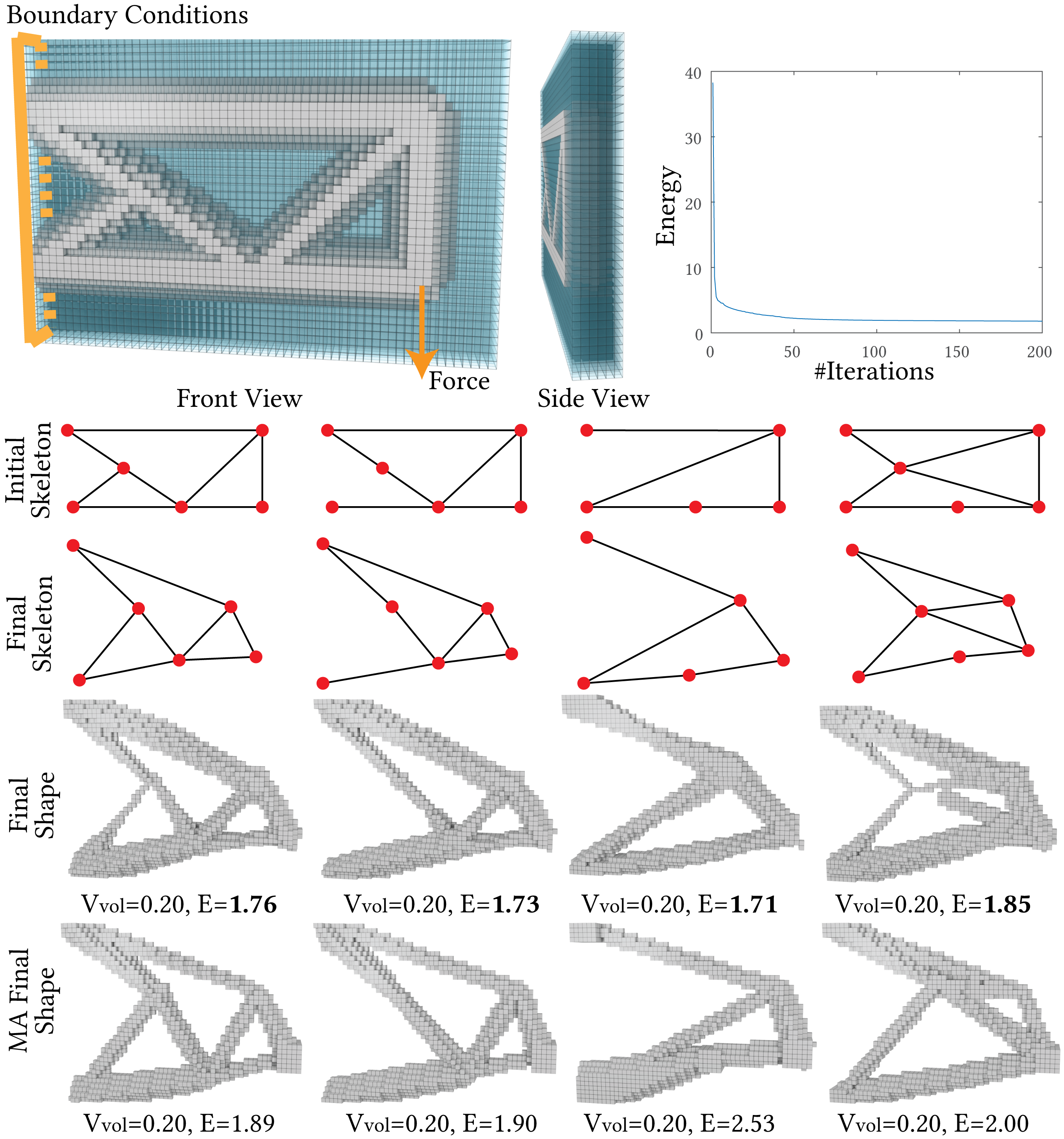
Figure 17. Results of shape optimization. We run shape optimization using our medial skeletal diagram with a similar setup to topology optimization (top left), but with four input skeletons as topology constraints. The optimization converges fast (top right), and each optimized shape shares the same topology as the corresponding input (bottom). Moreover, with our representation (Final Shape), we obtained a lower converged energy in all examples compared with the medial axis representation (MA Final Shape).

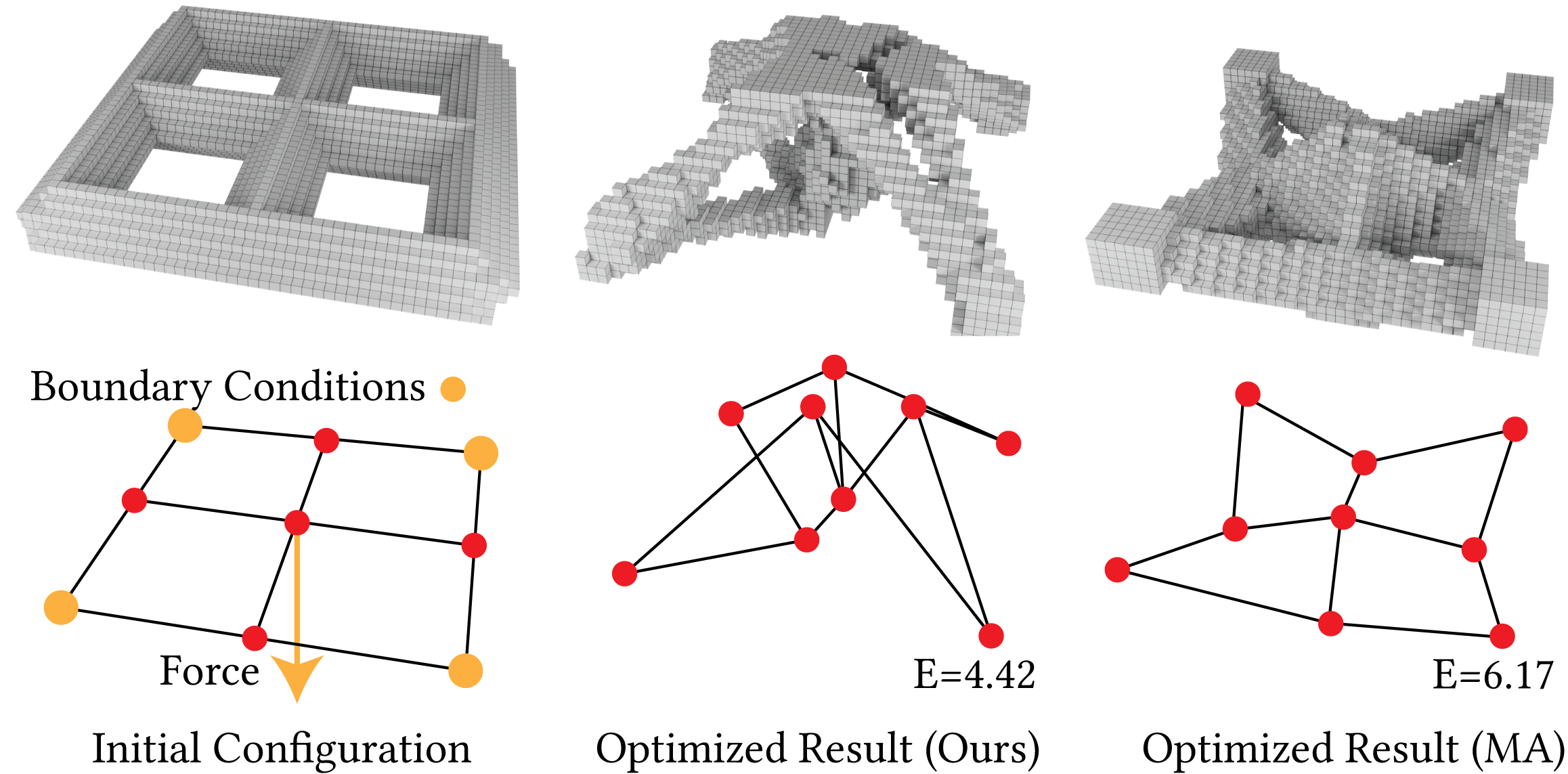
Figure 18. The result of shape optimization with a complex topology as constraints. Our representation is capable of optimizing shapes with user-defined topology constraints, a feature that is non-trivial to incorporate for voxel representation. Moreover, with our representation (middle), we obtained a lower converged energy in this complex example compared with the medial axis representation (right).

To substantiate this, we apply our representation to a topology-constrained shape optimization task. This task takes an initial 3D skeletal graph, which specifies the topology of the shape, and optimizes the shape to achieve a predefined objective while maintaining the same topological structure. We choose the objective to be compliance minimization, a well-known topology optimization task. The goal of this task is to optimize a shape that can withstand input load with minimal compliance given the maximal allowed material usage. Conventionally, such optimization is conducted within the space of a voxel grid, where each voxel carries a binary value to denote the presence of the material. Here, we re-frame the optimization within the space of our representation. We start by taking the initial 3D skeletal graph as the discrete structure of our medial skeletal diagram and constructing initial generalized enveloping primitives upon this discrete structure. The optimization variables are the continuous parameters of our medial skeletal diagram, which include the positions of the vertices and the radii of each primitive. Fig. 17 and 18 show the experimental setup.

The optimization problem is formulated as follows:

$$\operatorname*{arg\,min}_{\hat{\mathbf{v}},\hat{\mathbf{r}}}\ E(\mathbf{u},\hat{\mathbf{v}},\hat{\mathbf{r}})=\frac{1}{2}\mathbf{u}^{\intercal}\mathbf{K}(\mathbf{X})\mathbf{u},$$

s.t. $$\mathbf{K}(\mathbf{X})\mathbf{u}=\mathbf{f},$$

$$\mathbf{X}_{i}=\theta(x_{i};\hat{\mathbf{v}},\hat{\mathbf{r}}),\forall x_{i}\in\Omega$$

$$\sum\mathbf{X}_{i}\leq V_{\mathrm{vol}}\cdot|\Omega|,$$

$$\mathbf{u}_{\mathrm{BC}}=0,$$

where $\hat{\mathbf{v}}$ is the concatenation of the medial vertex positions, which in turn determines the locations of generalized enveloping primitives, $\hat{\mathbf{r}}$ is the concatenation of the radius values $\mathbf{r}$ of all primitives, $\mathbf{X}_{i}$ is the density of voxel $x_{i}$ in the given domain $\Omega$, $\mathbf{K}(\cdot)$ is the tangent stiffness matrix of a linear elastic material, $\mathbf{u}$ is the displacement of the shape under external force $\mathbf{f}$, $\mathbf{u}_{\mathrm{BC}}$ is the displacement of the grid points on the boundary condition, and $V_{\mathrm{vol}}$ is the desired volume fraction of the final shape relative to the total voxel space. We refer the readers to Chen et al. [2007] and Kumar [2023] for the definition of $\mathbf{K}(\cdot)$ and other standard aspects of the compliance minimization problem. Note that $\theta(x_{i};\hat{\mathbf{v}},\hat{\mathbf{r}})$ bridges the continuous parameters of our medial skeletal diagram with the voxel grid space, defined as

$$\theta(x_{i};\hat{\mathbf{v}},\hat{\mathbf{r}})=H(f(\bigcup_{k}-\mathcal{E}_{k}(x_{i};\mathcal{T}_{\mathcal{E}_{P}}(\hat{\mathbf{v}},\hat{\mathbf{r}})))).$$

Here, $\mathcal{E}_{k}(\cdot;\mathcal{T}_{\mathcal{E}_{P}}(\hat{\mathbf{v}},\hat{\mathbf{r}}))$ is the implicit function (as defined in Sec. 5.2) of the $k$-th generalized enveloping primitive $\mathcal{T}_{\mathcal{E}_{P}}$ constructed using $\hat{\mathbf{v}},\hat{\mathbf{r}}$. $f(\cdot)$ refers to Rvachev disjunction function [Chen et al., 2007] converting boolean compositions into a real-value function, where the sign of the output value indicates the boolean value of the input compositions: $f(\phi_{s}\cup\phi_{t})=\phi_{s}+\phi_{t}+\sqrt{\phi_{s}^{2}+\phi_{t}^{2}}$. $H(\cdot)$ is Heaviside step function. In essence, $\theta(x_{i};\hat{\mathbf{v}},\hat{\mathbf{r}})$ outputs a value of one for voxels within the union of primitives, and zero otherwise. We solve the optimization using gradient descent. Appendix A provides details of the gradient calculation.

We conduct two sets of experiments using the aforementioned formulation. The first set is to optimize shapes under the same boundary conditions and external forces within a voxel space of $60\times 40\times 6$ while maintaining topology constraints using four distinct user-defined skeletal graphs built upon a shared set of vertices. The input value $V_{\mathrm{vol}}$ is set to 0.2. The optimization successfully finds the minimum in all four scenarios, with each converging to a valid solution that matches the topology of the corresponding input skeletal graph. The optimized shapes, along with their compliance values, are shown in Fig. 17. Moreover, all minimizers from our representation are lower than those using the medial axis representation, with an average $14\%$ lower compliance value. The second experiment optimizes a shape within a larger voxel space $60\times 60\times 40$ using a more complex skeletal structure as input. The input value $V_{\mathrm{vol}}$ is set to $0.05$. The optimizer also successfully yields a structure with minimal compliance ($E=4.42$), versus minimal compliance values $6.17$ from the medial axis representation. The final result is shown in Fig. 18. These experimental results demonstrate the capability of our representation to perform shape optimization with user-defined topology constraints, a feature that is non-trivial to incorporate for voxel representation in a typical topology optimization setup. Further, it also produces superior results compared to existing work with medial axis representation [Bell et al., 2012]. In our implementation, we use $|\hat{\mathbf{r}}_{k}|=8$ for a medial vertex and $|\hat{\mathbf{r}}_{k}|=12$ for a medial edge, which results in a total of approximately $250$ DOFs in both examples – much smaller than the total number of voxels.

6.2.2. Shape Generation

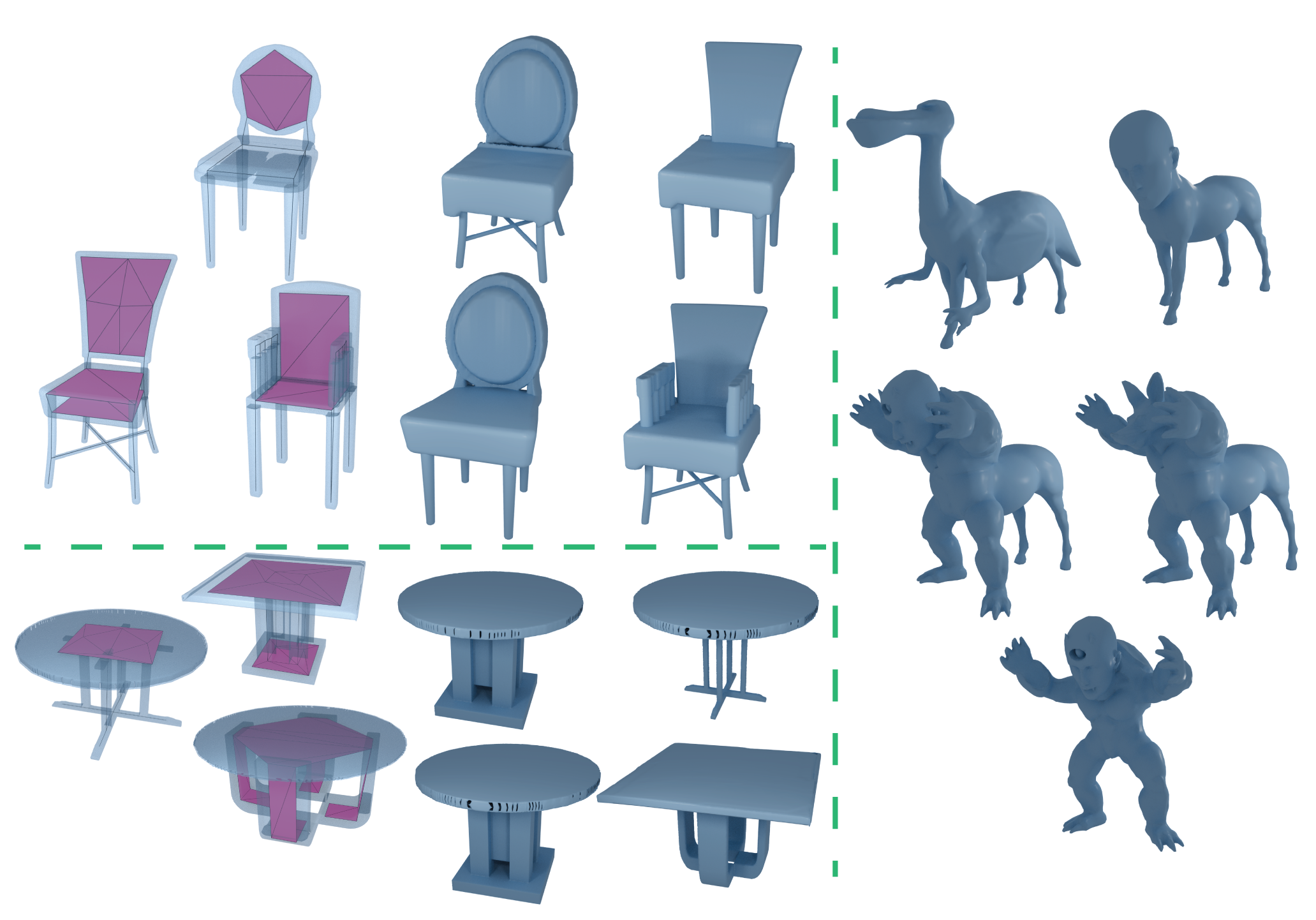
Figure 19. Results of shape generation. We use a cut-and-paste method based on our medial skeletal diagram to generate new shapes. The chairs and tables are generated from shapes provided in Mo et al. [2019], with each row showing outputs generated using three mesh inputs (left). The bottom row shows five generated shapes derived from the $100$ shape benchmark.

We use the cut-and-paste method employed in existing shape modeling techniques [Pandey et al., 2022] to generate new shapes from a given set of input shapes. We first construct the medial skeletal diagram for each shape in the input set. We then build a corpus of sub-skeletons by cutting subgraphs from these skeletons. To generate new shapes, we assemble these sub-skeletons, adding edges between them to ensure the resulting skeleton is a single connected component. New shapes are then generated by pasting and uniting the fitted generalized enveloping primitives from the input shapes. We use mesh boolean operations implemented from libigl to unite the primitives [Jacobson et al., 2018]. Using this process, we generate shapes from PartNet [Mo et al., 2019] and leverage the provided first-level part labels to perform the cutting on the skeleton. Fig. 19 illustrates the generated shapes for chairs and tables. This process of shape generation is remarkably straightforward and efficient, yet it ensures diverse changes in topology and geometry. In Fig. 19, we also showcase several generated shapes derived from the $100$ shapes benchmark. This streamlined process is made possible by the simplicity of the skeleton combined with the rich expressiveness of the primitives in our representation. In contrast, the medial axis representation demands a complex graph to accurately reconstruct the surface. Consequently, executing straightforward algorithms like the cut-and-paste method becomes challenging and necessitates considerable manual effort.

6.2.3. Mesh Decomposition

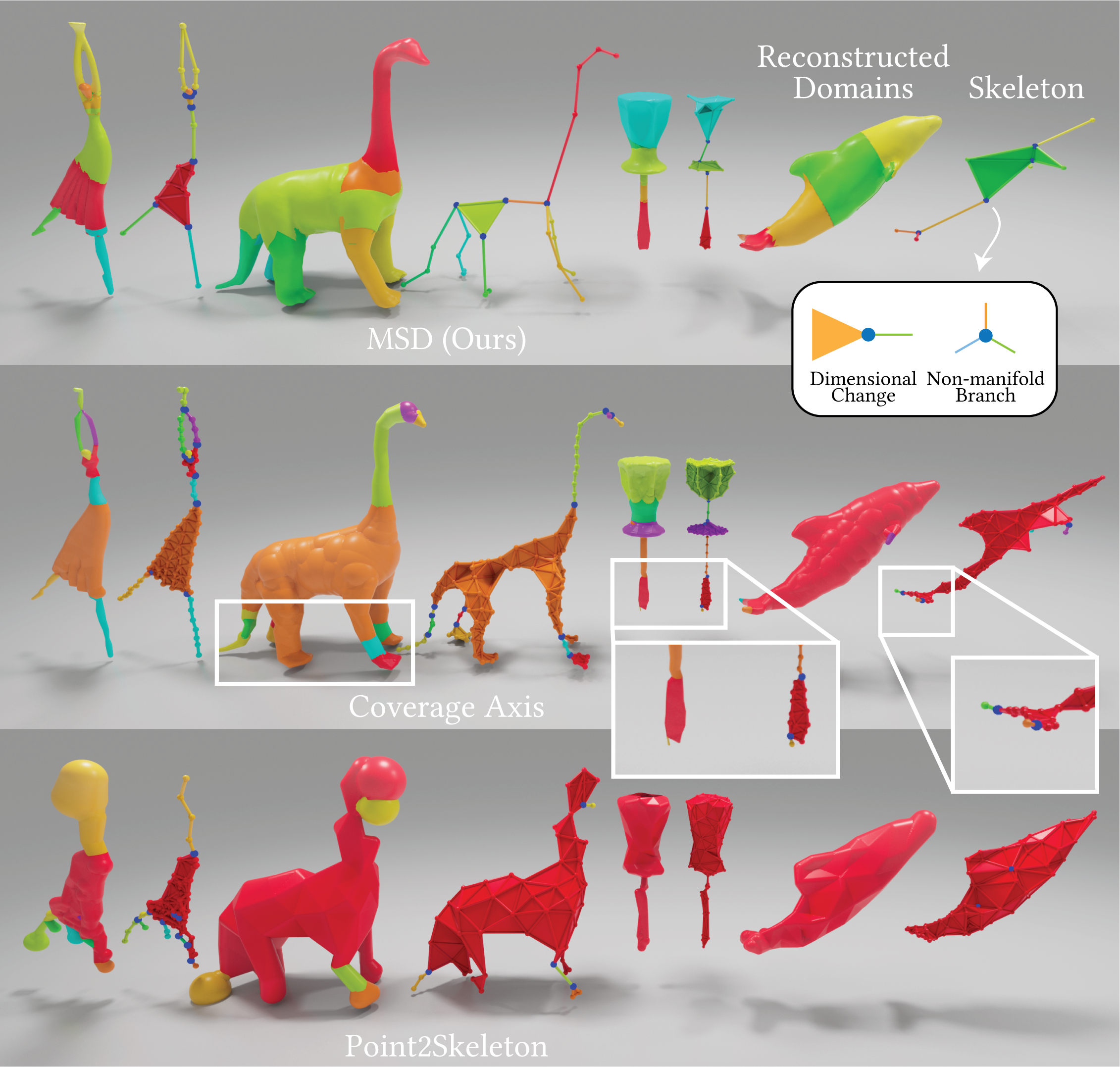
Figure 20. Domain Decomposition. We adopt the method from [Lin et al., 2021] for domain decomposition. Due to the simplicity of our skeleton and its precise shape reconstruction capabilities, our representation yields meaningful domain decomposition results. Although the coverage axis typically provides high-quality decomposition in many instances, it struggles to produce accurate decomposition in certain highlighted areas (white rectangles). While Point2Skeleton excels in generating high-quality decomposition for specific shapes, like chairs, as demonstrated in their paper [Lin et al., 2021], it falls short with more general shapes.

Due to the simplicity of our skeleton and high accuracy in reconstructing the shape, our representation can also be used to perform domain decomposition of the shape. Following the method from [Lin et al., 2021], we first identify the skeleton vertices that encounter a dimensional change on the neighboring elements or that are non-manifold vertices and then decompose the skeleton at these vertices. As shown in Fig. 20, we can generate a meaningful and concise decomposition of the mesh, while other methods fail to do so.

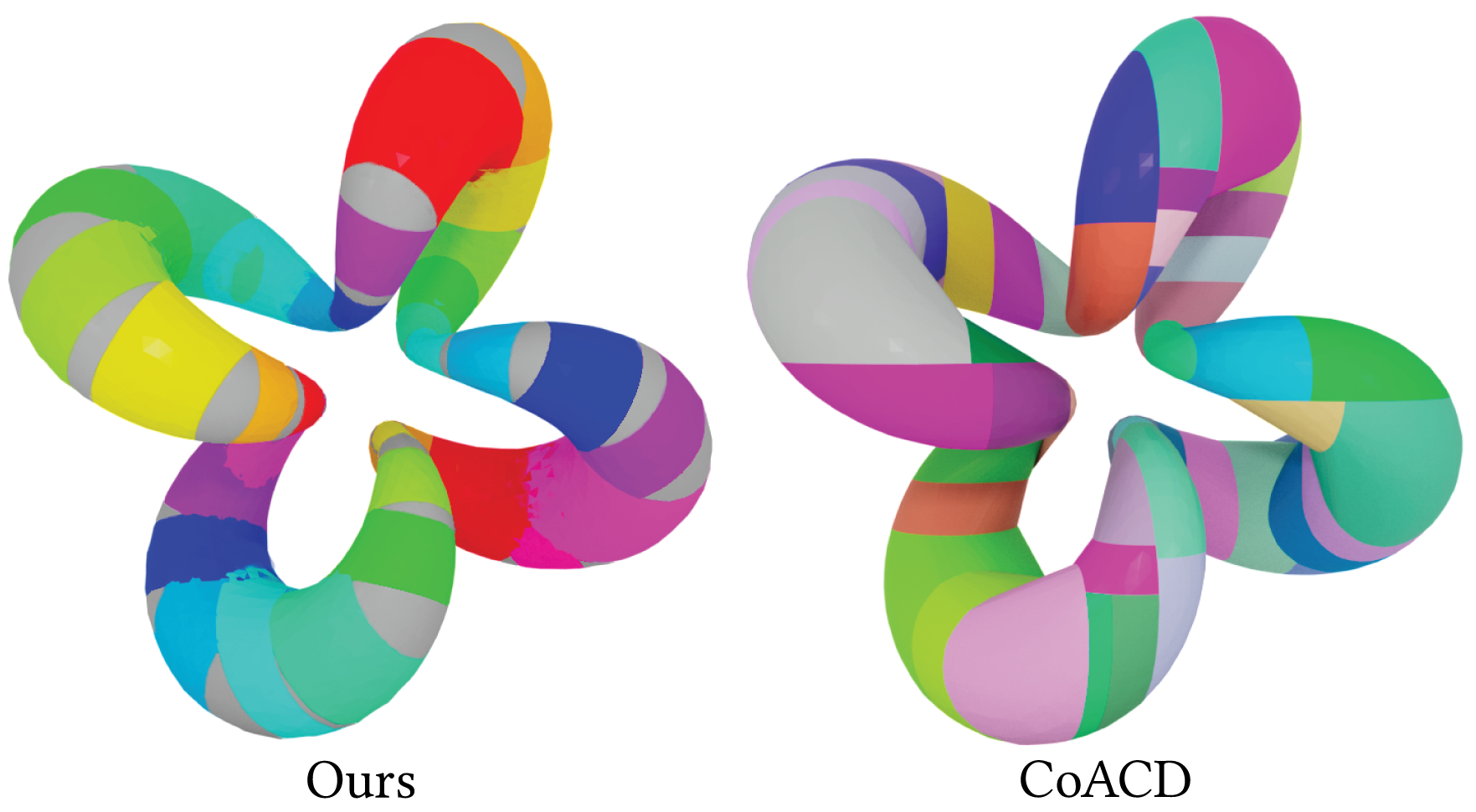
Figure 21. Comparison between medial skeletal diagram and CoACD on Knot example. The number of generalized enveloping primitives in our representation is smaller than the domains decomposed by CoACD.

Moreover, we compare the number of elements in our representation with the state-of-the-art domain decomposition method, CoACD [Wei et al., 2022]. Although these two methods do not share the same objective, a comparison can still be illuminating. Specifically, CoACD aims to decompose shapes into convex domains by cutting meshes with 3D planes, whereas our approach works by performing a union of all fitted primitives to represent the shape. Fig. 21 illustrates the comparison on the Knot example. While our method, unlike CoACD, does not ensure the convexity of each primitive, it outperforms in terms of simplicity, demonstrating a drastically reduced number of elements compared to CoACD. Furthermore, our method excels in capturing the topology of 3D shapes, a feature not adequately addressed by domain decomposition methods.

6.2.4. Mesh Alignment

Using our representation, we can ease non-rigid alignment between different shapes. To showcase its efficacy, we select four shapes from different species within the Animal3D dataset [Xu et al., 2023]. We then non-rigidly align the source mesh (highlighted in yellow) with the other three meshes (depicted in blue), as illustrated in Fig. 22. Instead of directly aligning the source mesh to the target, we first compute our MSD for each shape and then non-rigidly align their skeletons. Due to the simplicity of these skeletons, alignment is more straightforward than with surface meshes. Once the skeletons are aligned, the surface mesh is deformed according to the skeleton’s deformation. In our examples, we treat the skeleton as the kinematic object, with the surface mesh representing the surface of a tetrahedral mesh anchored to the skeleton. This mesh is then deformed using a physically-based simulation. The deformed mesh serves as an initial guess for the non-rigid alignment of the surface meshes, significantly reducing the manual effort needed to select landmark pairs between the source and target meshes.

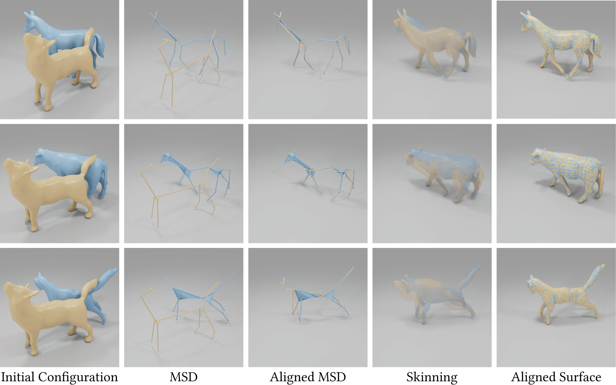
Figure 22. Non-rigid Alignment. Using our representation, one can initially align the medial skeletal diagrams to simplify subsequent surface non-rigid alignment. After the skeletons are matched, the surfaces deform in line with their corresponding skeletons, providing an initial estimate for the final non-rigid alignment. This preliminary alignment considerably eases the non-rigid alignment process for the surfaces, reducing the need for manual intervention.

6.2.5. Mesh Compression

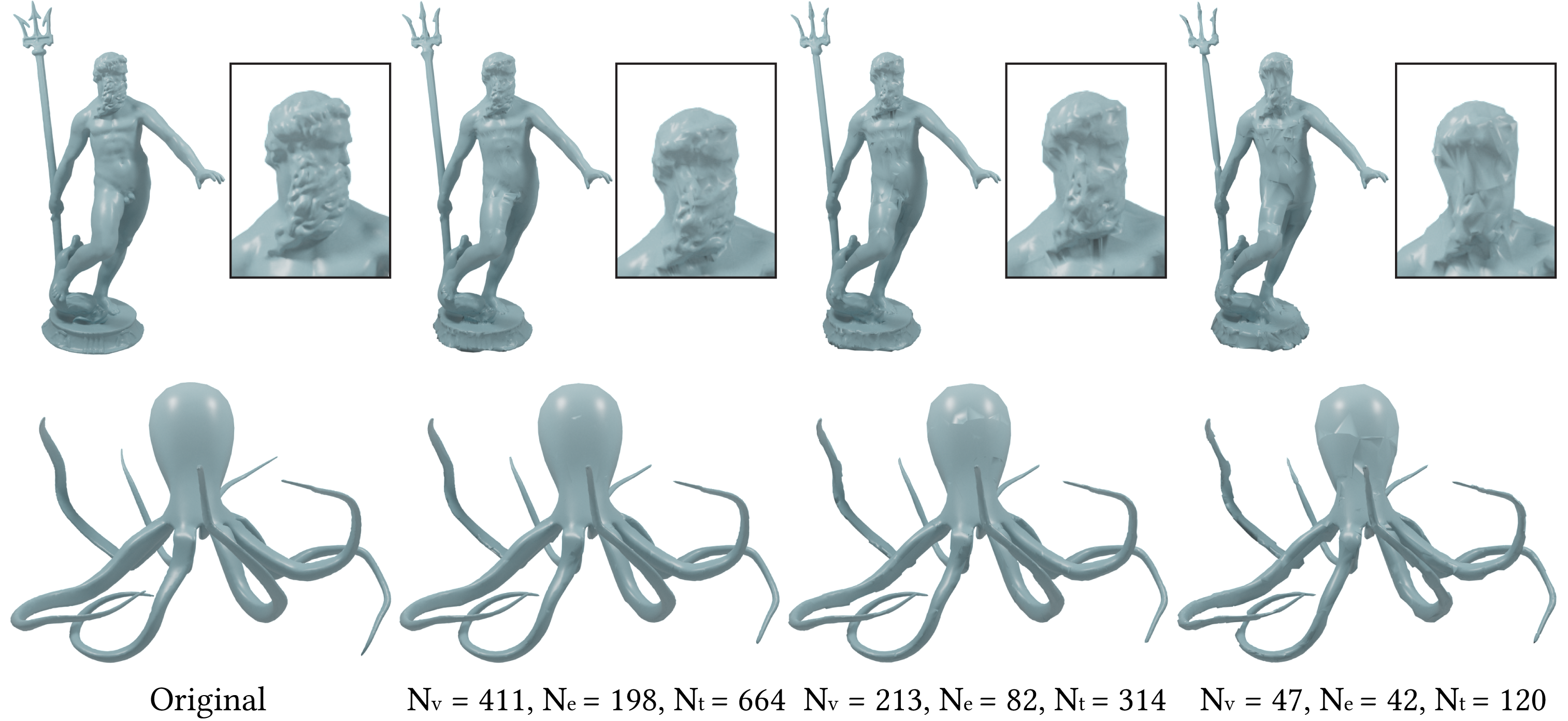
Figure 23. Mesh Compression. Our MSD can be easily used for mesh compression. For each primitive type, we define a canonical mesh with three different resolutions. Primitives at high resolution can be directly downsampled to lower resolutions using the predefined canonical mesh, thereby achieving mesh compression.

We also propose a simple approach to control the number of continuous parameters associated with each primitive, facilitating mesh compression. For each example shown in Fig. 23, we first compute its MSD. Subsequently, mesh compression is achieved by adjusting the mesh resolution for each primitive. For each primitive type, we define three canonical meshes with varying resolutions. Specifically, for a sphere mesh, the resolutions are $411$, $213$, and $47$; for a cylinder mesh, they are $198$, $82$, and $42$; and for a prism mesh, they are $664$, $314$, and $120$. Each calculated generalized enveloping primitive is mapped to its corresponding canonical mesh. As observed in Fig. 23, reducing the number of continuous parameters still yields a convincingly reconstructed surface.

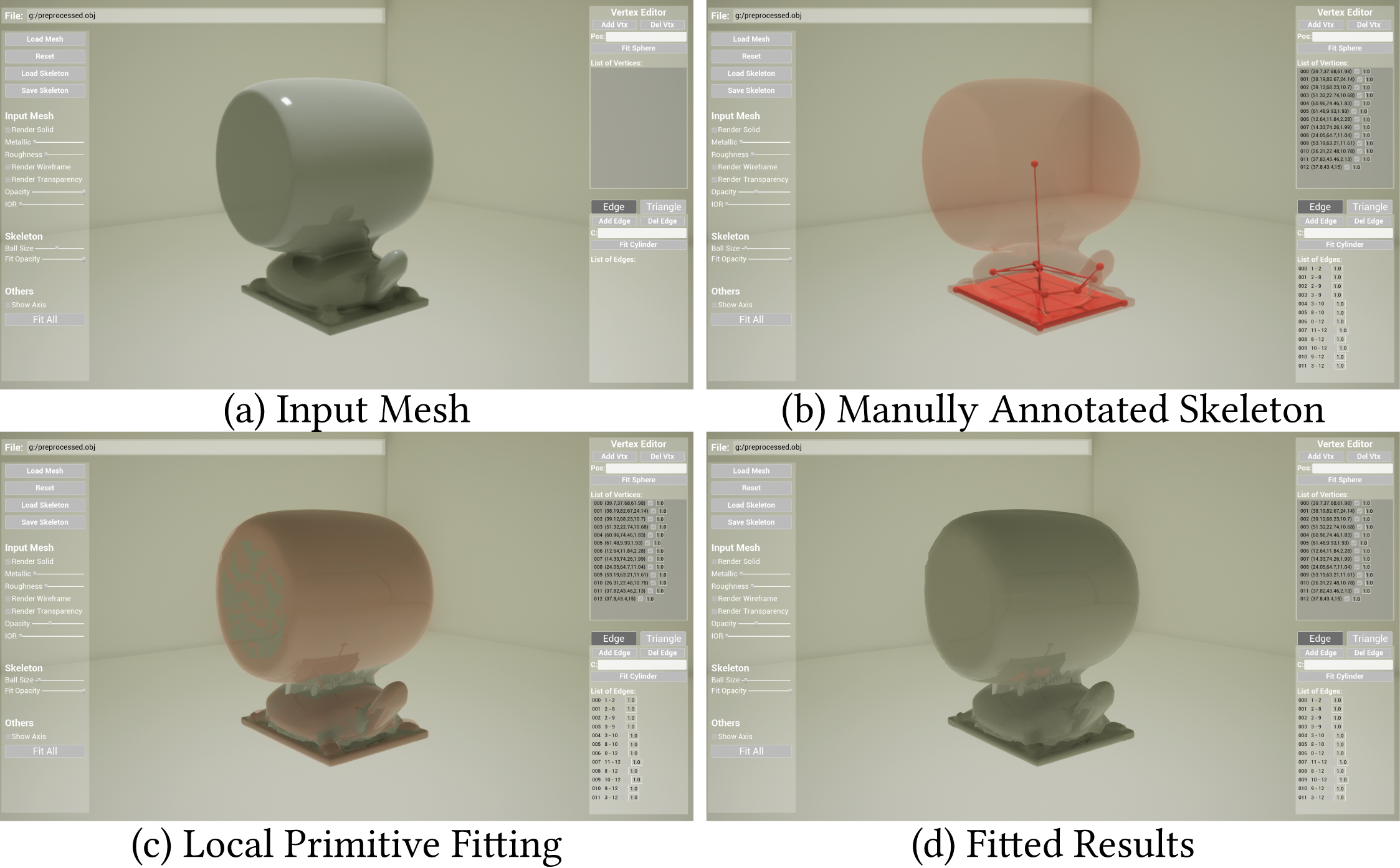
Figure 24. Constructing medial skeletal diagram using our GUI. Users can manually annotate all the skeletal elements and use our proposed local primitive fitting to obtain each primitive.

6.2.6. User Interface

The compact nature of our medial skeletal diagram offers users an intuitive and convenient method for shape modeling. To demonstrate it, we implement a graphical user interface (GUI). Within this GUI, users can create skeletal elements and apply our proposed local primitive fitting to represent a given input shape. As shown in Fig. 24, the user was able to manually construct a skeleton with $13$ vertices, $12$ edges, and $4$ triangles to represent the Drum shape. Moreover, users can manually identify and mark necessary skeletal feature points of the shape, such as topological features, and place points for an input mesh using our GUI. These selected points are then used as inputs for our construction pipeline which can automatically produce a high-quality skeleton and the reconstructed mesh. An example of a double torus is illustrated in Fig. 25.

6.3. Additional Results

We additionally show a gallery of additional results from the benchmark of $100$ shapes in Fig. 26 and 27. These results underscore the versatility of our method and its ability to handle a wide variety of shapes.

7. Limitations and Future Work

Our current approach does not guarantee topological preservation, which is also a limitation in the state-of-the-art work [Wang et al., 2022a, b]. A key reason for this limitation lies in the extreme sparsity of our medial skeletal diagram. The inherent sparsity of our representation contradicts the sufficient condition for maintaining homotopy, which demands that sampled points must be sufficiently dense to satisfy the $\epsilon$-sampling condition, as detailed in  [Amenta and Bern, 1998; Yan et al., 2009]. This leads to situations where the topology of the reconstructed 3D shape might be compromised. Future research directions may delve deeper into these topological considerations, investigating potential techniques or modifications to the current method that could ensure topological preservation, even with the sparse nature of our medial skeletal diagram.

In addition to the topological preservation issue, the computational approach for calculating the shortest path during the construction of the medial skeletal diagram could be optimized. We currently utilize Dijkstra’s algorithm. While it provides a functional solution, it is not the most ideal for this particular application as mentioned in [Wang et al., 2020; Xin et al., 2022]. A theoretically more suitable approach would be to employ geodesic Voronoi diagram (GVD). However, this presents a challenge due to the non-manifoldness of the medial axis, the space where GVD is computed. Future work could thus seek methods for replacing RVD with GVD in non-manifold domains. Possible avenues for this could include using a non-manifold Laplacian coupled with heat diffusion, as detailed in [Sharp and Crane, 2020]. Another potential solution could involve the development or adaptation of an exact geodesic distance calculator [Surazhsky et al., 2005].

Our current medial skeletal diagram consists solely of piecewise linear elements. Although this configuration has demonstrated solid performance, the inclusion of higher-order surfaces like polynomial elements [Marschner et al., 2021] could potentially enhance the representation further. Higher-order surfaces could provide more precise and compact coverage of intricate local regions, contributing to both the accuracy and efficiency of our representation.

Currently, the time efficiency of computing MSD is less than ideal. Future work that incorporates data-driven methods and graph generation may enhance computational speed, using our current method to supply training data pairs.

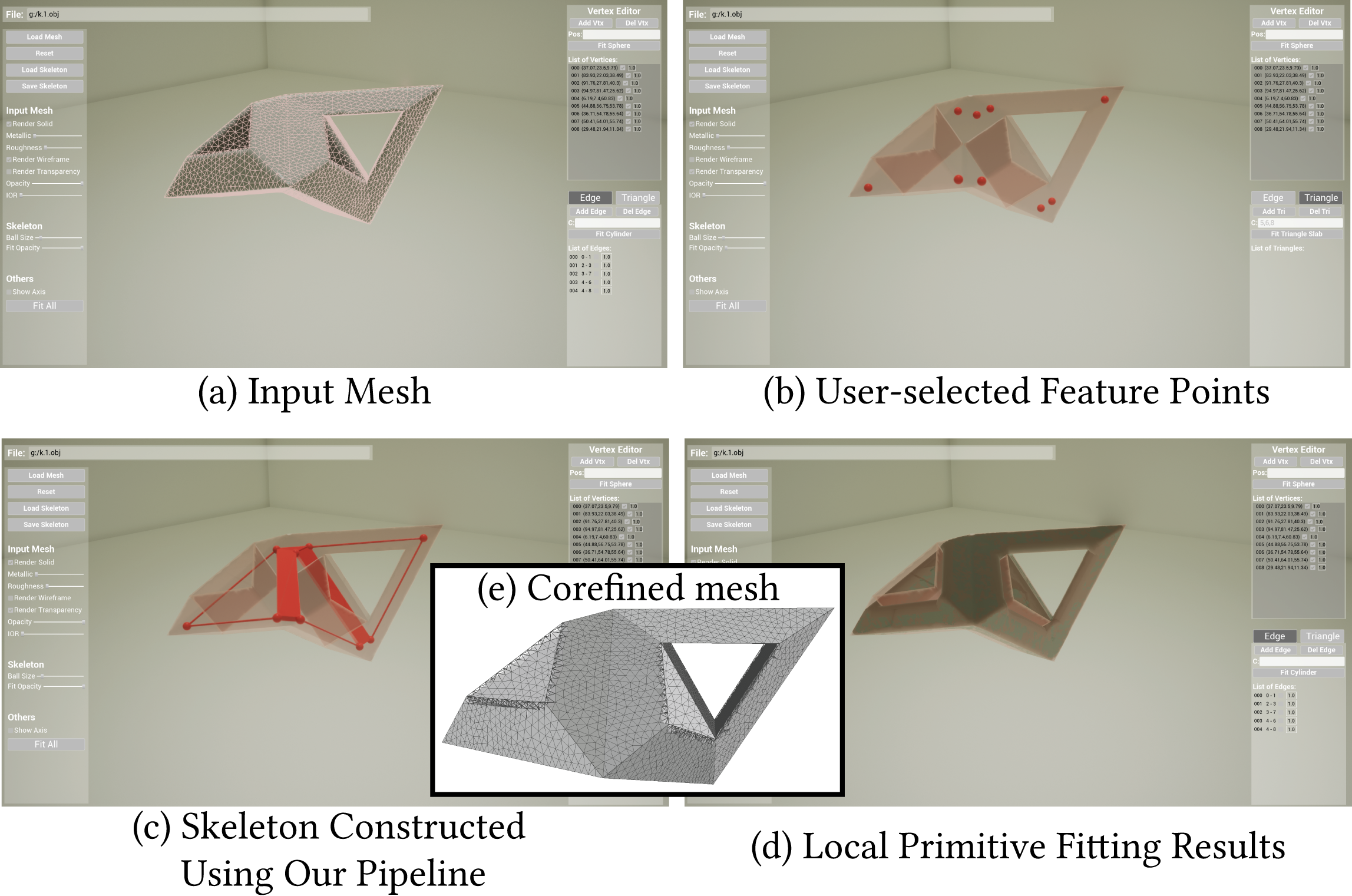
Figure 25. Constructing medial skeletal diagram with user-selected feature points using our GUI. Users can designate only the skeletal vertices where our medial skeletal diagram construction pipeline automatically produces the corresponding skeleton and the reconstructed mesh.

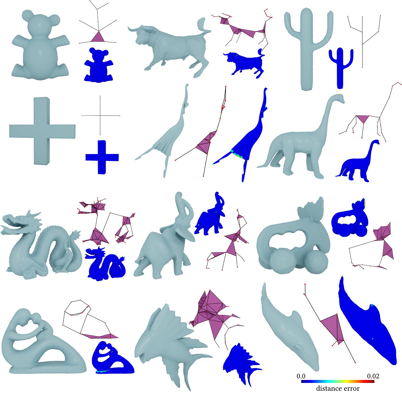
Figure 26. A gallery of more results of our medial skeletal diagram (part 1/2). For each sample, we show the reconstructed shape, the discrete skeleton, and the reconstruction error map on the input mesh.

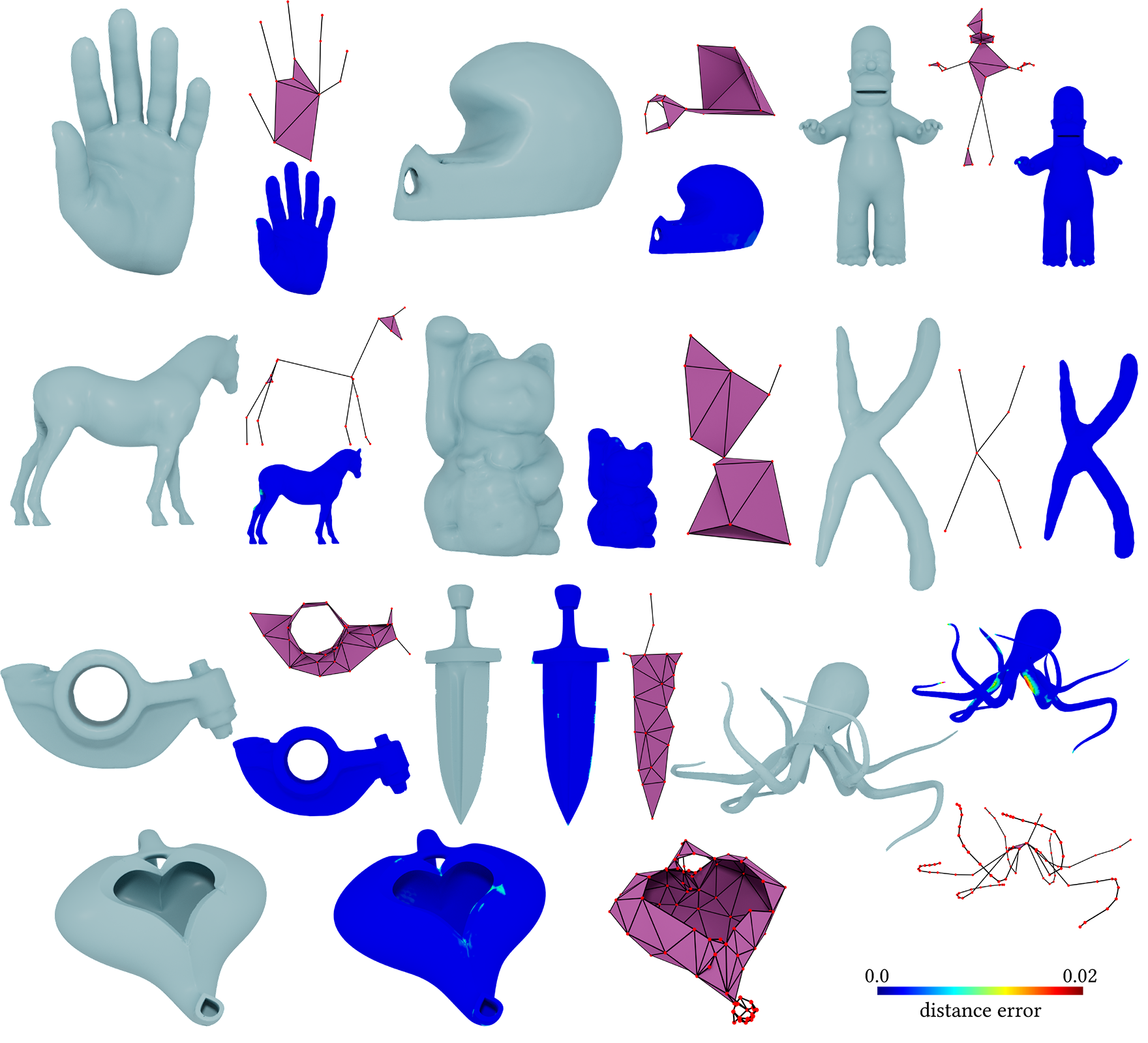
Figure 27. A gallery of more results of our medial skeletal diagram (part 2/2). For each sample, we show the reconstructed shape, the discrete skeleton, and the reconstruction error map on the input mesh.

8. Conclusion

In this paper, we present the medial skeletal diagram, a skeletal representation that strives for both compactness and completeness. Our approach significantly reduces the number of discrete elements while preserving completeness by augmenting the complexity of the continuous elements. Our medial skeletal diagram extends the medial axis by introducing generalized enveloping primitives which effectively cover complex local shape regions. We also present a computational pipeline to construct the medial skeletal diagram from an input shape by employing a local-global optimization paradigm to maximize shape coverage and minimize the count of discrete elements. A post-refinement process is conducted to guarantee an accurate match of our representation with the target mesh. We demonstrated the effectiveness of our method on a benchmark of $100$ shapes and highlighted its application in shape generation, shape optimization, and user-interactive design. Our future work will aim to incorporate data-driven methods into our approach, extending its applications to more shape analysis tasks including shape segmentation and recognition.

Appendix

Appendix A Shape Optimization Using Gradient Descent

We make the Heaviside step function differentiable by modifying $H(\cdot)$ as

(10) $$H(x)=\begin{cases}0\ &x<\gamma,\\ -\frac{1}{4\gamma^{3}}x^{3}+\frac{3}{4\gamma}x+0.5\ &-\gamma\leq x\leq\gamma,\\ 1\ &x>\gamma\end{cases},$$

where $\gamma$ is a small number. We choose $\gamma=0.01$ as the cell size of each voxel. The function is $C^{1}$ continuous in $\mathbb{R}$. Fig. 28 shows the plot of the function $H(\cdot)$.

To perform gradient descent, we first convert the inequality constraint into a quadratic energy term,

(11) $$E_{v}(\hat{\mathbf{v}},\hat{\mathbf{r}})=\begin{cases}\frac{w}{2}(\sum_{x_{i}}\frac{\theta(x_{i};\hat{\mathbf{v}},\hat{\mathbf{r}})}{|\Omega|}-V_{\mathrm{vol}})^{2}&\mathrm{if}\sum_{x_{i}}\frac{\theta(x_{i};\hat{\mathbf{v}},\hat{\mathbf{r}})}{|\Omega|}>V_{\mathrm{vol}},\\ 0&\mathrm{o.w.}\end{cases}$$

The energy is non-zero only if the current volume exceeds the user-defined one. Next, we differentiate the static equilibrium constraints

(12) $$\frac{\partial\mathbf{K}(\theta)}{\partial\theta}\mathbf{u}+\mathbf{K}(\theta)\frac{\partial\mathbf{u}}{\partial\theta}=0.$$

The gradient of the objective w.r.t. $(\hat{\mathbf{v}},\hat{\mathbf{r}})$ is

(13) $$\frac{dE}{d(\hat{\mathbf{v}},\hat{\mathbf{r}})} =\frac{\partial E}{\partial\mathbf{u}}\frac{\partial\mathbf{u}}{\partial(\hat{\mathbf{v}},\hat{\mathbf{r}})}+\frac{\partial E}{\partial(\hat{\mathbf{v}},\hat{\mathbf{r}})}$$

(14) $$=\left(-\frac{1}{2}\mathbf{u}^{T}\frac{\partial\mathbf{K}(\theta)}{\partial\theta}\mathbf{u}+wS^{T}(S\frac{\theta}{|\Omega|}-V_{\mathrm{vol}})\right)\frac{\partial\theta}{\partial(\hat{\mathbf{v}},\hat{\mathbf{r}})},$$

where $S$ is the summation linear operator. We apply gradient descent to optimize the objective of shape optimization. At each gradient descent iteration, we also perform a back-tracing line search to guarantee a decrease in the total energy. At each line search iteration, we first compute $\mathbf{K}$ from a new $(\hat{\mathbf{v}},\hat{\mathbf{r}})$ and then solve the static equilibrium to obtain $\mathbf{u}$. The energy is computed as $\frac{1}{2}\mathbf{u}^{\intercal}\mathbf{K}\mathbf{u}+E_{v}$.

Figure 28. The modified function $H(\cdot)$

References

- [1]
- Amenta and Bern [1998] Nina Amenta and Marshall Bern. 1998. Surface reconstruction by Voronoi filtering. In Proceedings of the fourteenth annual symposium on Computational geometry. 39–48.
- Amenta et al. [2001a] Nina Amenta, Sunghee Choi, and Ravi Krishna Kolluri. 2001a. The power crust. In Proceedings of the sixth ACM symposium on Solid modeling and applications. 249–266.
- Amenta et al. [2001b] Nina Amenta, Sunghee Choi, and Ravi Krishna Kolluri. 2001b. The power crust, unions of balls, and the medial axis transform. Computational Geometry 19, 2-3 (2001), 127–153.
- Attali et al. [2009] Dominique Attali, Jean-Daniel Boissonnat, and Herbert Edelsbrunner. 2009. Stability and computation of medial axes-a state-of-the-art report. Mathematical foundations of scientific visualization, computer graphics, and massive data exploration (2009), 109–125.
- Au et al. [2008] Oscar Kin-Chung Au, Chiew-Lan Tai, Hung-Kuo Chu, Daniel Cohen-Or, and Tong-Yee Lee. 2008. Skeleton extraction by mesh contraction. ACM transactions on graphics (TOG) 27, 3 (2008), 1–10.
- Bærentzen and Rotenberg [2021] Andreas Bærentzen and Eva Rotenberg. 2021. Skeletonization via local separators. ACM Transactions on Graphics (TOG) 40, 5 (2021), 1–18.
- Bærentzen et al. [2014] J Andreas Bærentzen, Rinat Abdrashitov, and Karan Singh. 2014. Interactive shape modeling using a skeleton-mesh co-representation. ACM Transactions on Graphics (TOG) 33, 4 (2014), 1–10.
- Bærentzen et al. [2023] J Andreas Bærentzen, Rasmus Emil Christensen, Emil Toftegaard Gæde, and Eva Rotenberg. 2023. Multilevel Skeletonization Using Local Separators. arXiv preprint arXiv:2303.07210 (2023).
- Baran and Popović [2007] Ilya Baran and Jovan Popović. 2007. Automatic rigging and animation of 3d characters. ACM Transactions on graphics (TOG) 26, 3 (2007), 72–es.
- Bell et al. [2012] Bryan Bell, Julian Norato, and Daniel Tortorelli. 2012. A geometry projection method for continuum-based topology optimization of structures. In 12th AIAA Aviation Technology, integration, and operations (ATIO) conference and 14th AIAA/ISSMO multidisciplinary analysis and optimization conference. 5485.
- Blum [1967] Harry Blum. 1967. A transformation for extracting new descriptions of shape. Models for the perception of speech and visual form (1967), 362–380.
- Borosán et al. [2012] Péter Borosán, Ming Jin, Doug DeCarlo, Yotam Gingold, and Andrew Nealen. 2012. Rigmesh: automatic rigging for part-based shape modeling and deformation. ACM Transactions on Graphics (TOG) 31, 6 (2012), 1–9.
- Bouaziz et al. [2014] Sofien Bouaziz, Sebastian Martin, Tiantian Liu, Ladislav Kavan, and Mark Pauly. 2014. Projective dynamics: Fusing constraint projections for fast simulation. ACM transactions on graphics (TOG) 33, 4 (2014), 1–11.
- Chaussard et al. [2011] John Chaussard, Michel Couprie, and Hugues Talbot. 2011. Robust skeletonization using the discrete -medial axis. Pattern Recognition Letters 32, 9 (2011), 1384–1394.
- Chazal and Lieutier [2005] Frédéric Chazal and André Lieutier. 2005. The “-medial axis”. Graphical models 67, 4 (2005), 304–331.
- Chen et al. [2007] Jiaqin Chen, Vadim Shapiro, Krishnan Suresh, and Igor Tsukanov. 2007. Shape optimization with topological changes and parametric control. International journal for numerical methods in engineering 71, 3 (2007), 313–346.
- Cohen-Steiner and Morvan [2003] David Cohen-Steiner and Jean-Marie Morvan. 2003. Restricted delaunay triangulations and normal cycle. In Proceedings of the nineteenth annual symposium on Computational geometry. 312–321.
- Culver et al. [2004] Tim Culver, John Keyser, and Dinesh Manocha. 2004. Exact computation of the medial axis of a polyhedron. Computer Aided Geometric Design 21, 1 (2004), 65–98.
- Dey et al. [1999] Tamal Dey, Herbert Edelsbrunner, Sumanta Guha, and Dmitry Nekhayev. 1999. Topology preserving edge contraction. Publications de l’Institut Mathématique 66 (1999).
- Dey and Zhao [2002] Tamal K Dey and Wulue Zhao. 2002. Approximate medial axis as a voronoi subcomplex. In Proceedings of the seventh ACM symposium on Solid modeling and applications. 356–366.
- Dey and Zhao [2004] Tamal K Dey and Wulue Zhao. 2004. Approximating the medial axis from the Voronoi diagram with a convergence guarantee. Algorithmica 38 (2004), 179–200.
- Dou et al. [2022] Zhiyang Dou, Cheng Lin, Rui Xu, Lei Yang, Shiqing Xin, Taku Komura, and Wenping Wang. 2022. Coverage Axis: Inner Point Selection for 3D Shape Skeletonization. In Computer Graphics Forum, Vol. 41. Wiley Online Library, 419–432.
- Edelsbrunner and Shah [1994] Herbert Edelsbrunner and Nimish R Shah. 1994. Triangulating topological spaces. In Proceedings of the tenth annual symposium on Computational geometry. 285–292.
- Fang et al. [2008] Rui Fang, Afzal Godil, Xiaolan Li, and Asim Wagan. 2008. A new shape benchmark for 3D object retrieval. In Advances in Visual Computing: 4th International Symposium, ISVC 2008, Las Vegas, NV, USA, December 1-3, 2008. Proceedings, Part I 4. Springer, 381–392.
- Foskey et al. [2003] Mark Foskey, Ming C Lin, and Dinesh Manocha. 2003. Efficient computation of a simplified medial axis. In Proceedings of the eighth ACM symposium on Solid modeling and applications. 96–107.
- Huang et al. [2013] Hui Huang, Shihao Wu, Daniel Cohen-Or, Minglun Gong, Hao Zhang, Guiqing Li, and Baoquan Chen. 2013. L1-medial skeleton of point cloud. ACM Trans. Graph. 32, 4 (2013), 65–1.
- Jacobson et al. [2018] Alec Jacobson, Daniele Panozzo, et al. 2018. libigl: A simple C++ geometry processing library. https://libigl.github.io/.
- Kumar [2023] Prabhat Kumar. 2023. HoneyTop90: A 90-line MATLAB code for topology optimization using honeycomb tessellation. Optimization and Engineering 24, 2 (2023), 1433–1460.
- Li et al. [2015] Pan Li, Bin Wang, Feng Sun, Xiaohu Guo, Caiming Zhang, and Wenping Wang. 2015. Q-mat: Computing medial axis transform by quadratic error minimization. ACM Transactions on Graphics (TOG) 35, 1 (2015), 1–16.
- Lieutier [2003] André Lieutier. 2003. Any open bounded subset of R n has the same homotopy type than its medial axis. In Proceedings of the eighth ACM symposium on Solid modeling and applications. 65–75.
- Lin et al. [2021] Cheng Lin, Changjian Li, Yuan Liu, Nenglun Chen, Yi-King Choi, and Wenping Wang. 2021. Point2skeleton: Learning skeletal representations from point clouds. In Proceedings of the IEEE/CVF conference on computer vision and pattern recognition. 4277–4286.
- Lin et al. [2020] Cheng Lin, Lingjie Liu, Changjian Li, Leif Kobbelt, Bin Wang, Shiqing Xin, and Wenping Wang. 2020. Seg-mat: 3d shape segmentation using medial axis transform. IEEE transactions on visualization and computer graphics 28, 6 (2020), 2430–2444.
- Livesu et al. [2012] Marco Livesu, Fabio Guggeri, and Riccardo Scateni. 2012. Reconstructing the curve-skeletons of 3D shapes using the visual hull. IEEE transactions on visualization and computer graphics 18, 11 (2012), 1891–1901.
- Lloyd [1982] Stuart Lloyd. 1982. Least squares quantization in PCM. IEEE transactions on information theory 28, 2 (1982), 129–137.
- Ma et al. [2003] Wan-Chun Ma, Fu-Che Wu, and Ming Ouhyoung. 2003. Skeleton extraction of 3D objects with radial basis functions. In 2003 Shape Modeling International. IEEE, 207–215.
- MacRobert [1967] Thomas Murray MacRobert. 1967. Spherical harmonics: An elementary treatise on harmonic functions, with applications. Vol. 98. Dover publications.
- Mamou [2016] Khaled Mamou. 2016. Volumetric Hierarchical Approximate Convex Decomposition. In Game Engine Gems 3, Eric Lengyel (Ed.). A K Peters, 141–158.
- Marie et al. [2016] Romain Marie, Ouiddad Labbani-Igbida, and El Mustapha Mouaddib. 2016. The delta medial axis: a fast and robust algorithm for filtered skeleton extraction. Pattern Recognition 56 (2016), 26–39.
- Marschner et al. [2021] Zoë Marschner, Paul Zhang, David Palmer, and Justin Solomon. 2021. Sum-of-squares geometry processing. ACM Transactions on Graphics (TOG) 40, 6 (2021), 1–13.
- Miklos et al. [2010] Balint Miklos, Joachim Giesen, and Mark Pauly. 2010. Discrete scale axis representations for 3D geometry. In ACM SIGGRAPH 2010 papers. 1–10.
- Milenkovic [1993] Victor Milenkovic. 1993. Robust Construction of the Voronoi Diagram of a Polyhedron.. In CCCG, Vol. 93. Citeseer, 473–478.
- Mo et al. [2019] Kaichun Mo, Shilin Zhu, Angel X Chang, Li Yi, Subarna Tripathi, Leonidas J Guibas, and Hao Su. 2019. Partnet: A large-scale benchmark for fine-grained and hierarchical part-level 3d object understanding. In Proceedings of the IEEE/CVF conference on computer vision and pattern recognition. 909–918.
- Munkres [2018] James R Munkres. 2018. Analysis on manifolds. CRC Press.
- Pandey et al. [2022] Karran Pandey, J Andreas Bærentzen, and Karan Singh. 2022. Face Extrusion Quad Meshes. In ACM SIGGRAPH 2022 Conference Proceedings. 1–9.
- Pizer et al. [2003] Stephen M Pizer, Kaleem Siddiqi, Gabor Székely, James N Damon, and Steven W Zucker. 2003. Multiscale medial loci and their properties. International Journal of Computer Vision 55 (2003).
- Rebain et al. [2019] Daniel Rebain, Baptiste Angles, Julien Valentin, Nicholas Vining, Jiju Peethambaran, Shahram Izadi, and Andrea Tagliasacchi. 2019. LSMAT least squares medial axis transform. In Computer Graphics Forum, Vol. 38. Wiley Online Library, 5–18.
- Rebain et al. [2021] Daniel Rebain, Ke Li, Vincent Sitzmann, Soroosh Yazdani, Kwang Moo Yi, and Andrea Tagliasacchi. 2021. Deep medial fields. arXiv preprint arXiv:2106.03804 (2021).
- Richardson and Kuester [1973] Joel A Richardson and JL Kuester. 1973. Algorithm 454: the complex method for constrained optimization [E4]. Commun. ACM 16, 8 (1973), 487–489.
- Saha et al. [2016] Punam K Saha, Gunilla Borgefors, and Gabriella Sanniti di Baja. 2016. A survey on skeletonization algorithms and their applications. Pattern recognition letters 76 (2016), 3–12.
- Schröder and Sweldens [1995] Peter Schröder and Wim Sweldens. 1995. Spherical wavelets: Efficiently representing functions on the sphere. In Proceedings of the 22nd annual conference on Computer graphics and interactive techniques. 161–172.
- Sharf et al. [2007] Andrei Sharf, Thomas Lewiner, Ariel Shamir, and Leif Kobbelt. 2007. On-the-fly curve-skeleton computation for 3d shapes. In Computer Graphics Forum, Vol. 26. Wiley Online Library, 323–328.
- Sharp and Crane [2020] Nicholas Sharp and Keenan Crane. 2020. A laplacian for nonmanifold triangle meshes. In Computer Graphics Forum, Vol. 39. Wiley Online Library, 69–80.
- Shen et al. [2011] Wei Shen, Xiang Bai, Rong Hu, Hongyuan Wang, and Longin Jan Latecki. 2011. Skeleton growing and pruning with bending potential ratio. Pattern Recognition 44, 2 (2011), 196–209.
- Sherbrooke et al. [1996] Evan C Sherbrooke, Nicholas M Patrikalakis, and Erik Brisson. 1996. An algorithm for the medial axis transform of 3D polyhedral solids. IEEE transactions on visualization and computer graphics 2, 1 (1996), 44–61.
- Simari and Singh [2005] Patricio D Simari and Karan Singh. 2005. Extraction and remeshing of ellipsoidal representations from mesh data.. In Graphics Interface. 161–168.
- Smythe [1988] William B Smythe. 1988. Static and dynamic electricity. (1988).
- Sobiecki et al. [2014] André Sobiecki, Andrei Jalba, and Alexandru Telea. 2014. Comparison of curve and surface skeletonization methods for voxel shapes. Pattern Recognition Letters 47 (2014), 147–156.
- Sud et al. [2005] Avneesh Sud, Mark Foskey, and Dinesh Manocha. 2005. Homotopy-preserving medial axis simplification. In Proceedings of the 2005 ACM symposium on Solid and physical modeling. 39–50.
- Sun et al. [2015] Feng Sun, Yi-King Choi, Yizhou Yu, and Wenping Wang. 2015. Medial meshes–a compact and accurate representation of medial axis transform. IEEE transactions on visualization and computer graphics 22, 3 (2015), 1278–1290.
- Surazhsky et al. [2005] Vitaly Surazhsky, Tatiana Surazhsky, Danil Kirsanov, Steven J Gortler, and Hugues Hoppe. 2005. Fast exact and approximate geodesics on meshes. ACM transactions on graphics (TOG) 24, 3 (2005), 553–560.
- Tagliasacchi et al. [2012] Andrea Tagliasacchi, Ibraheem Alhashim, Matt Olson, and Hao Zhang. 2012. Mean curvature skeletons. In Computer Graphics Forum, Vol. 31. Wiley Online Library, 1735–1744.
- Tagliasacchi et al. [2016] Andrea Tagliasacchi, Thomas Delame, Michela Spagnuolo, Nina Amenta, and Alexandru Telea. 2016. 3d skeletons: A state-of-the-art report. In Computer Graphics Forum, Vol. 35. Wiley Online Library, 573–597.
- Tang et al. [2019] Jiapeng Tang, Xiaoguang Han, Junyi Pan, Kui Jia, and Xin Tong. 2019. A skeleton-bridged deep learning approach for generating meshes of complex topologies from single rgb images. In Proceedings of the ieee/cvf conference on computer vision and pattern recognition. 4541–4550.
- Tierny et al. [2008] Julien Tierny, Jean-Philippe Vandeborre, and Mohamed Daoudi. 2008. Enhancing 3D mesh topological skeletons with discrete contour constrictions. The Visual Computer 24 (2008), 155–172.
- Wang et al. [2022a] Ningna Wang, Bin Wang, Wenping Wang, and Xiaohu Guo. 2022a. Computing Medial Axis Transform with Feature Preservation via Restricted Power Diagram. ACM Transactions on Graphics (TOG) 41, 6 (2022), 1–18.
- Wang et al. [2022b] Pengfei Wang, Zixiong Wang, Shiqing Xin, Xifeng Gao, Wenping Wang, and Changhe Tu. 2022b. Restricted Delaunay Triangulation for Explicit Surface Reconstruction. ACM Transactions on Graphics 41, 5 (2022), 1–20.
- Wang et al. [2020] Pengfei Wang, Shiqing Xin, Changhe Tu, Dongming Yan, Yuanfeng Zhou, and Caiming Zhang. 2020. Robustly computing restricted Voronoi diagrams (RVD) on thin-plate models. Computer Aided Geometric Design 79 (2020), 101848.
- Wei et al. [2022] Xinyue Wei, Minghua Liu, Zhan Ling, and Hao Su. 2022. Approximate convex decomposition for 3d meshes with collision-aware concavity and tree search. ACM Transactions on Graphics (TOG) 41, 4 (2022), 1–18.
- Wong et al. [2012] Sai-Keung Wong, Jau-An Yang, Tan-Chi Ho, Yu-Chieh Chen, and Jung-Hong Chuang. 2012. A skeleton-based approach for shape correspondence. In Proceedings of the 11th ACM SIGGRAPH International Conference on Virtual-Reality Continuum and its Applications in Industry. 329–336.
- Wu et al. [2015] Shihao Wu, Hui Huang, Minglun Gong, Matthias Zwicker, and Daniel Cohen-Or. 2015. Deep points consolidation. ACM Transactions on Graphics (ToG) 34, 6 (2015), 1–13.
- Xin et al. [2022] Shiqing Xin, Pengfei Wang, Rui Xu, Dongming Yan, Shuangmin Chen, Wenping Wang, Caiming Zhang, and Changhe Tu. 2022. SurfaceVoronoi: Efficiently Computing Voronoi Diagrams Over Mesh Surfaces with Arbitrary Distance Solvers. ACM Transactions on Graphics (TOG) 41, 6 (2022), 1–12.
- Xu et al. [2023] Jiacong Xu, Yi Zhang, Jiawei Peng, Wufei Ma, Artur Jesslen, Pengliang Ji, Qixin Hu, Jiehua Zhang, Qihao Liu, Jiahao Wang, et al. 2023. Animal3D: A Comprehensive Dataset of 3D Animal Pose and Shape. In Proceedings of the IEEE/CVF International Conference on Computer Vision. 9099–9109.
- Yan et al. [2009] Dong-Ming Yan, Bruno Lévy, Yang Liu, Feng Sun, and Wenping Wang. 2009. Isotropic remeshing with fast and exact computation of restricted Voronoi diagram. In Computer graphics forum, Vol. 28. Wiley Online Library, 1445–1454.
- Yan et al. [2018] Yajie Yan, David Letscher, and Tao Ju. 2018. Voxel cores: Efficient, robust, and provably good approximation of 3d medial axes. ACM Transactions on Graphics (TOG) 37, 4 (2018), 1–13.
- Yan et al. [2016] Yajie Yan, Kyle Sykes, Erin Chambers, David Letscher, and Tao Ju. 2016. Erosion thickness on medial axes of 3D shapes. ACM Transactions on Graphics (TOG) 35, 4 (2016), 1–12.
- Yang et al. [2020] Baorong Yang, Junfeng Yao, Bin Wang, Jianwei Hu, Yiling Pan, Tianxiang Pan, Wenping Wang, and Xiaohu Guo. 2020. P2MAT-NET: Learning medial axis transform from sparse point clouds. Computer Aided Geometric Design 80 (2020), 101874.
- Zhou et al. [2015] Yang Zhou, Kangxue Yin, Hui Huang, Hao Zhang, Minglun Gong, and Daniel Cohen-Or. 2015. Generalized cylinder decomposition. ACM Trans. Graph. 34, 6 (2015), 171–1.