The effect of solar wind on the charged particles’ diffusion coefficients

Abstract

The transport of energetic charged particles through magnetized plasmas is ubiquitous in interplanetary space and astrophysics, and the important physical quantities are the along-field and cross-field spatial diffusion coefficients of energetic charged particles. In this paper, the influence of solar wind on particle transport is investigated. Using the focusing equation, we obtain along- and cross-field diffusion coefficient accounting for the solar wind effect. For different conditions, the relative importance of solar wind effect to diffusion are investigated. It is shown that when energetic charged particles are close to the sun, for along-field diffusion the solar wind effect needs to be taken into account. These results are important for studying energetic charged particle transport processes in the vicinity of the sun.

1 INTRODUCTION

The charged energetic particles emitted by the sun, known as solar energetic particles (SEPs), have crucial impacts on the environment of interplanetary and planetary space (Schlickeiser, 2002; Reames, 2017). For example, SEPs can cause geomagnetic and ionospheric storms on the Earth, and even pose a threat to the safe operation of the ground power systems and cause leaks in underground oil pipelines. In addition, these energetic particles can reduce the reliability of spacecraft-borne detectors and endanger the health of astraurants and aircrew (Lanzerotti, 2017; Mertens et al., 2018). The turbulent magnetized plasmas in the interplanetary space, e.g., the solar wind, have a significant impact on the transport of solar energetic particles. Therefore, it is extremely important to investigate the propagation of solar energetic particles through the solar wind (Jokipii, 1966; Zhang, 1999; Schlickeiser, 2002; Matthaeus et al., 2003; Qin, 2007; Schlickeiser et al, 2007; Schlickeiser & Shalchi, 2008; Shalchi, 2010; Qin & Zhang, 2014; Wang & Qin, 2015; Zhang & Zhao, 2017; Zhang et al., 2019; Zhao et al., 2017).

Due to the interaction with the background and superposed turbulent magnetic fields, the motion of charged energetic particles can be modelled as two components of motions, i.e., the helical motion around the mean magnetic field lines and the superposed stochastic one (Schlickeiser, 2002; Shalchi, 2009). Therefore, various statistical methods have to be utilized in related studies (Jokipii, 1966; Schlickeiser, 2002; Matthaeus et al., 2003; Shalchi, 2009, 2010, 2020b). The well-known Master equation in statistical physics, which provides the most fundamental description of the transport of charged energetic particles through magnetized plasmas, is too complicated to be used in analytical investigations (Schlickeiser, 2002; Shalchi, 2009). Therefore, in the previous papers the relatively simple equations, such as the Fokker-Planck equation, have been widely used in plasma physics, astrophysics and space physics. The focusing equation, the special version of the Fokker-Planck equation, has been extensively employed in the research of the energetic particle transport in the heliosphere and the magnetosphere (Skilling, 1971; Schlickeiser, 2002; Qin et al., 2005, 2006; Zhang et al., 2009; Dröge et al., 2010; Zuo et al., 2011; Wang et al., 2012; Qin et al., 2013; Zuo et al., 2013; Wang et al., 2014; Zhang et al., 2019; Qin & Qi, 2020).

The focusing equation includes all the important transport effects of SEPs in solar wind plasmas, e.g., the pitch-angle diffusion, the cross-field diffusion, the spatial convection, the adiabatic cooling, the adiabatic focusing, and so on, among which, the spatial convection, the adiabatic cooling, and the adiabatic focusing are affected by solar wind velocity effects (Skilling, 1971; Schlickeiser, 2002; Forbes et al., 2006; Shalchi, 2009; Zhang & Zhao, 2017; Wijsen et al., 2019; Zhang et al., 2019; Bian & Emslie, 2020). These effects in the focusing equation are not isolated from each other, but have mutual influence. The along- and cross-field spatial diffusion are very important transport processes of energetic charged particles, so they are widely studied in plasma physics (Schlickeiser, 2002; Qin, 2007; Shalchi, 2009; Qin & Zhang, 2014; Qin & Shalchi, 2014; Shalchi, 2020b). In addition, the impacts of along-field adiabatic focusing effect on the along- and cross-field diffusion have been extensively studied (Roelof, 1969; Earl, 1976; Kunstmann, 1979; Beeck & Wibberenz, 1986; Bieber & Burger, 1990; Kota, 2000; Schlickeiser & Shalchi, 2008; Shalchi, 2011; Litvinenko, 2012a, b; Shalchi & Danos, 2013; He & Schlickeiser, 2014; Wang & Qin, 2016; Wang et al., 2017; Wang & Qin, 2018, 2019).

For the along-field diffusion, three different definitions of diffusive coefficient have been proposed in the past decades, i.e., the displacement variance definition

$$\kappa_{zz}^{DV}=\frac{1}{2}\lim_{t\rightarrow t_{\infty}}\frac{\mathrm{d}\sigma^{2}}{\mathrm{d}t}$$ (1)

with the first- and second-order moments of charged particle distribution function, the Fick’s law definition

$$\kappa_{zz}^{FL}=\frac{J}{X}$$ (2)

with $X=\partial{F}/\partial{z}$, and the TGK formula definition

$$\kappa_{zz}^{TGK}=\int_{0}^{\infty}dt\langle v_{z}(t)v_{z}(0)\rangle.$$ (3)

If the mean magnetic field is uneven along the field lines, it has been proved that different definitions of along-field diffusion coefficient are not equivalent to each other, i.e., $\kappa_{zz}^{DV}$, rather than $\kappa_{zz}^{FL}$ and $\kappa_{zz}^{TGK}$, is the most appropriate definition (Wang & Qin, 2018, 2019). In addition, it is demonstrated that the cross-field diffusion coefficient $\kappa_{\perp}$ is modified by along-field non-uniformity of the mean magnetic field (Wang et al., 2017). Moreover, the influence of along-field adiabatic focusing on the momentum transport have also been investigated (Schlickeiser & Shalchi, 2008; Litvinenko & Schlickeiser, 2011; Wang & Qin, 2021).

Cross-field diffusion, i.e., perpendicular diffusion, is another crucial transport process for charged particles in both space physics and laboratory plasma physics. Cross-field diffusion coefficient, which is the important parameter describing perpendicular transport, has been widely investigated in previous studies (Matthaeus et al., 2003; Shalchi, 2010; Qin & Zhang, 2014; Shalchi, 2017, 2019, 2020a, 2020b, 2021a, 2021b, 2022). A large number of studies have demonstated that along-field diffusion has a strong influence on perpendicular transport (Matthaeus et al., 2003; Shalchi et al., 2004, 2006; Shalchi, 2008, 2010, 2017, 2018, 2019, 2020a, 2020b, 2021a). In addition, along-field adiabatic focusing effect is another factor influencing cross-field diffusion (Wang et al., 2017). However, the effect of solar wind on cross-field diffusion has not been investigated in the previous paper. In this paper, we also explore this problem.

The remainder of this paper is organized as follows. In Section 2, the focusing equation that satisfies particle number conservation is introduced. In Section 3, the along- and cross-field diffusion coefficients of energetic charged particles including solar wind effects are derived. In Section 4, the influence of the solar wind effect on along-field diffusion is explored, with the dimensionless quantities determining the relative importance of the solar wind effect to diffusion transport derived. In Section 5, the effect of solar wind on cross-field diffusion is expored. We conclude and summarize our results in Section 6.

2 The focusing equation

The Fokker-Planck equation is formulated as follows (Duderstadt & Martin, 1979; Huang & Ding, 2008; Zank, 2014)

$$\frac{\partial{f}}{\partial{t}}+\nabla\cdot\left(\bm{u}f\right)+\nabla_{p}\cdot\left(\bm{a}f\right)= \nabla\cdot\left(\kappa_{1}\cdot\nabla f\right)+\nabla_{p}\cdot\left(\kappa_{1}^{p}\cdot\nabla_{p}f\right)+\nabla\cdot\left[\kappa_{21}\cdot\nabla\left(\kappa_{22}\cdot\nabla f\right)\right]$$ (4)

$$+\nabla_{p}\cdot\left[\kappa_{21}^{p}\cdot\nabla_{p}\left(\kappa_{22}^{p}\cdot\nabla_{p}f\right)\right]+\cdots.$$

Here, $f=f(\bm{r},\bm{p},t)$ is the distribution function of charged energetic particles, $t$ is time, $\bm{u}$ is particle velocity, and $\bm{a}$ is particle acceleration. In addition, the operators $\nabla$ and $\nabla_{p}$ are the spatial and momentum Laplacians, respectively. For simplicity, only the first- and second-order derivative terms of the Fokker-Planck equation are usually retained (Huang & Ding, 2008), thus Equation (4) becomes

$$\frac{\partial{f}}{\partial{t}}+\nabla\cdot\left(\bm{u}f\right)+\nabla_{p}\cdot\left(\bm{a}f\right)=\nabla\cdot\left(\kappa\cdot\nabla f\right)+\nabla_{p}\cdot\left(\kappa_{p}\cdot\nabla_{p}f\right).$$ (5)

In general, the terms of the first- and second-order derivative in Equation (5) can describe most of the important specific physical effects of energetic particle transport in solar wind plasmas, e.g., pitch-angle scattering, cross-field diffusion, along-field adiabatic focusing, adiabatic cooling, along-field spatial convection, etc. To encompasses all of the aforementioned physical processes, the focusing equation becomes the Fokker-Planck equation,

$$\frac{\partial{f}}{\partial{t}}=\nabla\cdot\left(\kappa_{\perp}\cdot\nabla f\right)-\nabla\cdot\left[\left(u\mu\hat{\bm{b}}+\bm{V}\right)f\right]+\frac{\partial{}}{\partial{\mu}}\left(D_{\mu\mu}\frac{\partial{f}}{\partial{\mu}}\right)$$

$$+\frac{1}{p^{2}}\frac{\partial{}}{\partial{p}}\Bigg{\{}p^{3}\Bigg{[}\frac{1-\mu^{2}}{2}\left(\nabla\cdot\bm{V}-\hat{\bm{b}}\hat{\bm{b}}:\nabla\bm{V}\right)+\mu^{2}\hat{\bm{b}}\hat{\bm{b}}:\nabla\bm{V}\Bigg{]}f\Bigg{\}}$$

$$+\frac{\partial{}}{\partial{\mu}}\Bigg{\{}\frac{1-\mu^{2}}{2}\Bigg{[}-\frac{u}{L}-\mu\left(\nabla\cdot\bm{V}-3\hat{\bm{b}}\hat{\bm{b}}:\nabla\bm{V}\right)\Bigg{]}f\Bigg{\}},$$ (6)

where $\kappa_{\perp}$ is the perpendicular diffusion coefficient tensor, $u$ is the particle speed, $\mu$ is pitch-angle cosine, $\hat{\bm{b}}$ is the unit vector along the background magnetic field, $p$ is the magnitude of momentum, $D_{\mu\mu}(\mu)$ is the pitch-angle diffusion coefficient, $L=\left(\hat{\bm{b}}\cdot\nabla\ln B\right)^{-1}$ with solar mean magneitc field $B$ is the characteristic length of the adiabatic focusing, and $\bm{V}$ is the solar wind velocity. The latter equation satisfies the conservation law of particle number, and the detailed derivative is shown in Appendix A. For convenience, the focusing equation can be rewritten as follows

$$\frac{\partial{f}}{\partial{t}}=\nabla\cdot\left(\kappa_{\perp}\cdot\nabla f\right)-\nabla\cdot\left[\left(u\mu\hat{\bm{b}}+\bm{V}\right)f\right]+\frac{\partial{}}{\partial{\mu}}\left(D_{\mu\mu}\frac{\partial{f}}{\partial{\mu}}\right)+\frac{\partial{}}{\partial{\mu}}\left[\frac{u\left(1-\mu^{2}\right)}{2L}f\right]$$

$$+\frac{1}{p^{2}}\frac{\partial{}}{\partial{p}}\Bigg{\{}p^{3}\Bigg{[}\frac{1-\mu^{2}}{2}\left(\frac{\partial{V_{x}}}{\partial{x}}+\frac{\partial{V_{y}}}{\partial{y}}\right)+\mu^{2}\frac{\partial{V_{z}}}{\partial{z}}\Bigg{]}f\Bigg{\}}-\frac{\partial{}}{\partial{\mu}}\Bigg{[}\mu\left(\frac{\partial{V_{x}}}{\partial{x}}+\frac{\partial{V_{y}}}{\partial{y}}-2\frac{\partial{V_{z}}}{\partial{z}}\right)f\Bigg{]}.$$ (7)

The derivation details from Equation (6) to (7) are shown in Appendix B.

3 The diffusion coefficients including solar wind effects

In this section, we explore the diffusion coefficients of energetic charged particles including solar wind effects.

3.1 The along-field diffusion coefficient including solar wind effects

Firstly, we derive the along-field diffusion coefficient formula of energetic particles including solar wind.

3.1.1 The simplified Fokker-Planck equation

For simplificty, the effect of solar wind spatial gradient are ignored. Moreover, by performing the integration $\int\mathrm{d}x\int\mathrm{d}y$ on Equation (7), we find

$$\frac{\partial{f_{a}}}{\partial{t}}=-u\mu\frac{\partial{f_{a}}}{\partial{z}}-\frac{\partial{}}{\partial{z}}\left(\int\mathrm{d}x\int\mathrm{d}yV_{z}f\right)+\frac{\partial{}}{\partial{\mu}}\left[D_{\mu\mu}\frac{\partial{f_{a}}}{\partial{\mu}}-\frac{u\left(1-\mu^{2}\right)}{2L}f_{a}\right].$$ (8)

Here, $f_{a}(z,\mu,t)=\int\mathrm{d}x\int\mathrm{d}yf(x,y,z,\mu,t)$ is the distribution function. Now, we obtain the simplified Fokkerr-Planck equation.

3.1.2 The anisotropic distribution function $g_{a}(z,\mu,t)$

The distribution function of charged energetic particles can be divided into the isotropic part $F_{a}$, which satisfies

$$F_{a}=\frac{1}{2}\int_{-1}^{1}\mathrm{d}\mu f_{a},$$ (9)

and the anisotropic component, which satisfies the condition

$$\int_{-1}^{1}\mathrm{d}\mu g_{a}=0.$$ (10)

That is, the following formula holds

$$f_{a}=F_{a}+g_{a},$$ (11)

By integrating Equation (8) over $\mu$ from $-1$ to $1$, we can obtain

$$\frac{\partial{F_{a}}}{\partial{t}}=-\frac{u}{2}\frac{\partial{}}{\partial{z}}\int_{-1}^{1}\mathrm{d}\mu\mu g_{a}-\frac{\partial{}}{\partial{z}}\left(\int\mathrm{d}x\int\mathrm{d}yV_{z}F\right).$$ (12)

Here, $F=\int_{-1}^{1}\mathrm{d}\mu f/2$ is employed. In addition, the boundary condition $D_{\mu\mu}(\mu=\pm 1)=0$ is also used. Similarly, integrating Equation (8) over $\mu$ from $-1$ to $\mu$, we obtain

$$\frac{\partial{F_{a}}}{\partial{t}}(\mu+1) +\frac{\partial{}}{\partial{t}}\int_{-1}^{\mu}\mathrm{d}\nu g_{a}=-u\frac{\mu^{2}-1}{2}\frac{\partial{F_{a}}}{\partial{z}}-u\frac{\partial{}}{\partial{z}}\int_{-1}^{\mu}\mathrm{d}\nu\nu g_{a}-(\mu+1)\frac{\partial{}}{\partial{z}}\left(\int\mathrm{d}x\int\mathrm{d}yV_{z}F\right)$$ (13)

$$-\frac{\partial{}}{\partial{z}}\left(\int\mathrm{d}x\int\mathrm{d}yV_{z}\int_{-1}^{\mu}\mathrm{d}\nu g(\nu)\right)+D_{\mu\mu}\frac{\partial{g_{a}}}{\partial{\mu}}-\frac{u\left(1-\mu^{2}\right)}{2L}F_{a}-\frac{u\left(1-\mu^{2}\right)}{2L}g_{a}$$

with $g(x,y,z,\mu,t)=f(x,y,z,\mu,t)-F(x,y,z,t)$. Equation (13) can be rewritten as

$$\frac{\partial{g_{a}}}{\partial{\mu}}+\frac{u\left(1-\mu^{2}\right)g_{a}}{2D_{\mu\mu}L}+\frac{u\left(1-\mu^{2}\right)}{2D_{\mu\mu}}\left(\frac{\partial{F_{a}}}{\partial{z}}+\frac{F_{a}}{L}\right)=\Phi_{a}(\mu)$$ (14)

with

$$\Phi_{a}(\mu)= \frac{1}{D_{\mu\mu}}\Bigg{[}\frac{\partial{F_{a}}}{\partial{t}}(\mu+1)+\frac{\partial{}}{\partial{t}}\int_{-1}^{\mu}\mathrm{d}\nu g_{a}$$ (15)

$$+u\frac{\partial{}}{\partial{z}}\int_{-1}^{\mu}\mathrm{d}\nu\nu g_{a}+(\mu+1)\frac{\partial{}}{\partial{z}}\left(\int\mathrm{d}x\int\mathrm{d}yV_{z}F\right)+\frac{\partial{}}{\partial{z}}\left(\int\mathrm{d}x\int\mathrm{d}yV_{z}\int_{-1}^{\mu}\mathrm{d}\nu g(\nu)\right)\Bigg{]}$$

To continue, Equation (14) can be rewritten as (He & Schlickeiser, 2014; Wang & Qin, 2018, 2019)

$$\frac{\partial{}}{\partial{\mu}}\Bigg{\{}\Bigg{[}g_{a}(\mu)+L\left(\frac{\partial{F_{a}}}{\partial{z}}+\frac{F_{a}}{L}\right)\Bigg{]}e^{-M(\mu)}\Bigg{\}}=e^{-M(\mu)}\Phi_{a}(\mu)$$ (16)

with

$$M(\mu) = -\frac{u}{2L}\int_{-1}^{\mu}d\nu\frac{1-\nu^{2}}{D_{\nu\nu}(\nu)},$$ (17)

By integrating Equation (16) over $\nu$ from $-1$ to $\mu$, we can obtain the anisotropic distribution function as follows

$$g_{a}(\mu)=-L\left(\frac{\partial{F_{a}}}{\partial{z}}+\frac{F_{a}}{L}\right)\left[1-\frac{2e^{M(\mu)}}{\int_{-1}^{1}d\mu e^{M(\mu)}}\right]+e^{M(\mu)}\left[R_{a}(\mu)-\frac{\int_{-1}^{1}d\mu e^{M(\mu)}R_{a}(\mu)}{\int_{-1}^{1}d\mu e^{M(\mu)}}\right]$$ (18)

with

$$R_{a}(\mu)=\int_{-1}^{\mu}d\nu e^{-M(\nu)}\Phi_{a}(\nu).$$ (19)

3.1.3 The governing equation of the isotropic distribution function $F_{a}(z,t)$

In order to derive the governing equation of the isotropic distribution function $F_{a}(z,t)$, we have to deduce the following integral

$$\frac{u}{2}\frac{\partial{}}{\partial{z}}\int_{-1}^{1}\mathrm{d}\mu\mu g_{a} =\left(u\frac{\partial{F_{a}}}{\partial{z}}+uL\frac{\partial^{2}{F_{a}}}{\partial{z^{2}}}\right)\frac{\int_{-1}^{1}\mathrm{d}\mu\mu e^{M(\mu)}}{\int_{-1}^{1}d\mu e^{M(\mu)}}$$ (20)

$$+\frac{u}{2}\int_{-1}^{1}\mathrm{d}\mu\mu e^{M(\mu)}\left[\frac{\partial{}}{\partial{z}}R_{a}(\mu)-\frac{1}{\int_{-1}^{1}d\mu e^{M(\mu)}}\int_{-1}^{1}d\mu e^{M(\mu)}\frac{\partial{}}{\partial{z}}R_{a}(\mu)\right].$$

The latter formula shows that the derivative of $R_{a}(z,\mu,t)$ with respect to $z$ has to be deduced

$$\frac{\partial{}}{\partial{z}}R_{a}(\mu)= \frac{\partial^{2}{F_{a}}}{\partial{z}\partial{t}}\int_{-1}^{\mu}d\nu\frac{e^{-M(\nu)}}{D_{\nu\nu}}(\nu+1)+\int_{-1}^{\mu}d\nu\frac{e^{-M(\nu)}}{D_{\nu\nu}}(\nu+1)\frac{\partial^{2}{}}{\partial{z^{2}}}\left(\int\mathrm{d}x\int\mathrm{d}yV_{z}F\right)$$ (21)

$$+\int_{-1}^{\mu}d\nu\frac{e^{-M(\nu)}}{D_{\nu\nu}}\frac{\partial^{2}{}}{\partial{t}\partial{z}}\int_{-1}^{\nu}\mathrm{d}\rho\int\mathrm{d}x\int\mathrm{d}yV_{z}F+u\int_{-1}^{\mu}d\nu\frac{e^{-M(\nu)}}{D_{\nu\nu}}\frac{\partial^{2}{}}{\partial{z^{2}}}\int_{-1}^{\nu}\mathrm{d}\rho\rho g_{a}$$

$$+\int_{-1}^{\mu}d\nu\frac{e^{-M(\nu)}}{D_{\nu\nu}}\frac{\partial^{2}{}}{\partial{z^{2}}}\left(\int\mathrm{d}x\int\mathrm{d}yV_{z}\int_{-1}^{\nu}\mathrm{d}\rho g_{a}\right).$$

With Equations (20) and (21), the governing equation of the isotropic distribution function can be found

$$\frac{\partial{F_{a}}}{\partial{t}}= -\frac{\partial{}}{\partial{z}}\left(\int\mathrm{d}x\int\mathrm{d}yV_{z}F_{a}\right)-\kappa_{z}\frac{\partial{F_{a}}}{\partial{z}}+\kappa_{zz}\frac{\partial^{2}{F_{a}}}{\partial{z^{2}}}+\kappa_{tz}\frac{\partial^{2}{F_{a}}}{\partial{t}\partial{z}}+\kappa_{zz}^{V}\frac{\partial^{2}{}}{\partial{z^{2}}}\left(\int\mathrm{d}x\int\mathrm{d}yV_{z}F_{a}\right)$$ (22)

with and

$$\kappa_{z}=-u\frac{\int_{-1}^{1}d\mu\mu e^{M(\mu)}}{\int_{-1}^{1}d\mu e^{M(\mu)}},$$ (23)

$$\kappa_{zz}=-uL\frac{\int_{-1}^{1}\mathrm{d}\mu\mu e^{M(\mu)}}{\int_{-1}^{1}d\mu e^{M(\mu)}}$$

$$+\frac{u^{2}}{2}\int_{-1}^{1}\mathrm{d}\mu\mu e^{M(\mu)}\int_{-1}^{\mu}d\nu\frac{e^{-M(\nu)}}{D_{\nu\nu}}\int_{-1}^{\nu}\mathrm{d}\rho\rho\left[1-\frac{2e^{M(\rho)}}{\int_{-1}^{1}d\mu e^{M(\mu)}}\right]$$

$$-\frac{u^{2}}{2}\frac{\int_{-1}^{1}\mathrm{d}\mu\mu e^{M(\mu)}}{\int_{-1}^{1}d\mu e^{M(\mu)}}\int_{-1}^{1}d\mu e^{M(\mu)}\int_{-1}^{\mu}d\nu\frac{e^{-M(\nu)}}{D_{\nu\nu}}\int_{-1}^{\nu}\mathrm{d}\rho\rho\left[1-\frac{2e^{M(\rho)}}{\int_{-1}^{1}d\mu e^{M(\mu)}}\right],$$ (24)

$$\kappa_{tz}=-\frac{u}{2}\int_{-1}^{1}\mathrm{d}\mu\mu e^{M(\mu)}\int_{-1}^{\mu}d\nu e^{-M(\nu)}\frac{\nu+1}{D_{\nu\nu}}+\frac{u}{2}\frac{\int_{-1}^{1}\mathrm{d}\mu\mu e^{M(\mu)}}{\int_{-1}^{1}d\mu e^{M(\mu)}}\int_{-1}^{1}d\mu e^{M(\mu)}\int_{-1}^{\mu}d\nu e^{-M(\nu)}\frac{\nu+1}{D_{\nu\nu}}$$

$$-\frac{u}{2}\int_{-1}^{1}\mathrm{d}\mu\mu e^{M(\mu)}\int_{-1}^{\mu}d\nu\frac{e^{-M(\nu)}}{D_{\nu\nu}}\int_{-1}^{\nu}\mathrm{d}\rho\left(\frac{2e^{M(\rho)}}{\int_{-1}^{1}d\mu e^{M(\mu)}}-1\right)$$

$$+\frac{u}{2}\frac{\int_{-1}^{1}\mathrm{d}\mu\mu e^{M(\mu)}}{\int_{-1}^{1}d\mu e^{M(\mu)}}\int_{-1}^{1}d\mu e^{M(\mu)}\int_{-1}^{\mu}d\nu\frac{e^{-M(\nu)}}{D_{\nu\nu}}\int_{-1}^{\nu}\mathrm{d}\rho\left(\frac{2e^{M(\rho)}}{\int_{-1}^{1}d\mu e^{M(\mu)}}-1\right)$$ (25)

$$\kappa_{zz}^{V}=\frac{u}{2}\frac{\int_{-1}^{1}\mathrm{d}\mu\mu e^{M(\mu)}}{\int_{-1}^{1}d\mu e^{M(\mu)}}\int_{-1}^{1}d\mu e^{M(\mu)}\int_{-1}^{\mu}d\nu\frac{e^{-M(\nu)}}{D_{\nu\nu}}(\nu+1)$$

$$-\frac{u}{2}\int_{-1}^{1}\mathrm{d}\mu\mu e^{M(\mu)}\int_{-1}^{\mu}d\nu\frac{e^{-M(\nu)}}{D_{\nu\nu}}(\nu+1).$$ (26)

Here, only the terms containing the first- and second-order derivatives are retained. In fact, the higher-order derivative terms do not affect the results obtained in this article (Wang & Qin, 2018, 2019).

3.1.4 The along-field diffusion coefficient formula

To derive the formula of mean square displacement definition, we have to obtain the first- and second-order moments of the isotropic distribution function, which are shown as follows

$$\frac{\mathrm{d}}{\mathrm{d}t}\left\langle z\right\rangle=\left\langle V_{z}\right\rangle+\kappa_{z},$$ (27)

$$\frac{\mathrm{d}}{\mathrm{d}t}\left\langle z^{2}\right\rangle=2\left\langle zV_{z}\right\rangle+2\kappa_{z}\langle z\rangle+2\kappa_{zz}-2\kappa_{tz}\frac{\mathrm{d}}{\mathrm{d}t}\langle z\rangle+2\kappa_{zz}^{V}\left\langle V_{z}\right\rangle.$$ (28)

Combining the latter formulas gives

$$\frac{1}{2}\frac{\mathrm{d}\sigma^{2}}{\mathrm{d}t}=\frac{1}{2}\frac{\mathrm{d}}{\mathrm{d}t}\left(\left\langle z^{2}\right\rangle-\langle z\rangle^{2}\right)=T_{1}-T_{2}+T_{3}+T_{4}$$ (29)

with

$$T_{1}=\kappa_{zz},$$ (30)

$$T_{2}=\kappa_{tz}\kappa_{z},$$ (31)

$$T_{3}=\zeta=\left\langle zV_{z}\right\rangle-\langle z\rangle\left\langle V_{z}\right\rangle,$$ (32)

$$T_{4}=\left(\kappa_{zz}^{V}-\kappa_{tz}\right)\left\langle V_{z}\right\rangle.$$ (33)

From Equations (32) and (33), we can find that the mean square displacement definition of along-field diffusion coefficient includes the solar wind and adiabatic focusing effects. According to the results obtained by Wang & Qin (2019), the term $T_{4}$ is approximately equal to zero. Thus, Equation (29) becomes

$$\frac{1}{2}\frac{\mathrm{d}\sigma^{2}}{\mathrm{d}t}=\frac{1}{2}\frac{\mathrm{d}}{\mathrm{d}t}\left(\left\langle z^{2}\right\rangle-\langle z\rangle^{2}\right)=T_{1}-T_{2}+T_{3}.$$ (34)

Note that if we only consider adiabatic focusing, Equation (34) becomes

$$\frac{1}{2}\frac{\mathrm{d}\sigma^{2}}{\mathrm{d}t}=T_{1}-T_{2}=\kappa_{zz}-\kappa_{tz}\kappa_{z},$$ (35)

which is identical to the result derived by Wang & Qin (2018).

3.2 The cross-field diffusion coefficient including solar wind effects

Next, we derive the cross-field diffusion coefficient of energetic charged particles including solar wind effect.

3.2.1 The govering equation of isotropic distribution function

The starting point of the investigation in this subsection is also the focusing equation, which is displayed in Section 2. For Equation (7), by ignoring the terms containing spatial derivaitve of solar wind speed and integrating over $\mu$ from $-1$ to $1$, we can obtain the governing equation of isotropic distribution function, which is given as follows

$$\frac{\partial{F^{\prime}}}{\partial{t}}=\nabla\cdot\left(\kappa_{\perp}\cdot\nabla F^{\prime}\right)-\frac{u}{2}\frac{\partial{}}{\partial{z}}\int_{-1}^{1}\mathrm{d}\mu\mu g-\nabla\cdot\left(\bm{V}F^{\prime}\right)$$ (36)

with

$$F^{\prime}=\frac{1}{2}\int_{-1}^{1}\mathrm{d}\mu f.$$ (37)

Here, $g(x,y,z,\mu,t)$ is the anisotropic distribution function. Performing integrating $\int\mathrm{d}y\int\mathrm{d}z$ on Equation (36) yields

$$\frac{\partial{F_{b}}}{\partial{t}}=\frac{\partial{}}{\partial{x}}\left(\kappa_{\perp}\frac{\partial{F_{b}}}{\partial{x}}\right)-\frac{\partial{}}{\partial{x}}\left(\int\mathrm{d}y\int\mathrm{d}zV_{x}F^{\prime}\right).$$ (38)

Here, $F_{b}=F(x,t)$ is the isotropic distribution function satisfying the following formula

$$F_{b}=\frac{1}{2}\int_{-1}^{1}\mathrm{d}\mu\int\mathrm{d}y\int\mathrm{d}zf.$$ (39)

3.2.2 The mean square displacement definition of perpendicular diffusion in $x$ direction

From Equation (38), the first- and second-order moments of charged particle distribution function can be obtained as

$$\frac{\mathrm{d}}{\mathrm{d}t}\langle x\rangle=\int\mathrm{d}x\int\mathrm{d}y\int\mathrm{d}zV_{x}F^{\prime}=\left\langle V_{x}\right\rangle,$$ (40)

$$\frac{\mathrm{d}}{\mathrm{d}t}\left\langle x^{2}\right\rangle=2\kappa_{\perp}+2\int\mathrm{d}x\int\mathrm{d}y\int\mathrm{d}zxV_{x}F’=2\kappa_{\perp}+2\left\langle xV_{x}\right\rangle.$$ (41)

Combining the latter formulas gives

$$\kappa_{xx}^{DV}=\frac{1}{2}\frac{\mathrm{d}\sigma_{x}^{2}}{\mathrm{d}t}=\frac{1}{2}\frac{d}{dt}\left(\langle x^{2}\rangle-\langle x\rangle^{2}\right)=\kappa_{\perp}+\eta$$ (42)

with

$$\eta=\left\langle xV_{x}\right\rangle-\langle x\rangle\left\langle V_{x}\right\rangle.$$ (43)

Here, $\kappa_{\perp}=\kappa_{xx}^{FL}$ is the Fick’s law definition. In addition, $\eta$ is the solar wind effect on the cross-field diffusion. Thus, Equation (43) indicates that the cross-field diffusion is affected by solar wind effect.

In the following, we would discuss the influence of solar wind on along- and cross-field diffusion, i.e., Equations (32) and (43), with the typical parameter values, e.g., solar wind speed $V\sim 3\times 10^{5}$ m/s, the solar rotation speed $\omega\sim 3\times 10^{-6}$ /s, the energetic proton speed $u\sim 10^{7}$ m/s, the particle parallel mean free path $\lambda\sim 10^{10}$ m, and the parameter $\lambda_{\perp}\equiv 3\kappa_{\perp}/u=10^{9}$ m.

4 The influence of solar wind on along-field diffusion

In this section, based on Equation (34) we discuss the solar wind effect on along-field diffusion of energetic charged particles. If we only consider solar wind effect, Equation (34) is simplifies as

$$\kappa_{zz}^{DV}=\frac{1}{2}\frac{\mathrm{d}\sigma^{2}}{\mathrm{d}t}=T_{1}+T_{3}=\kappa_{zz}+\zeta,$$ (44)

with

$$\zeta=\left\langle zV_{z}\right\rangle-\left\langle z\right\rangle\left\langle V_{z}\right\rangle.$$ (45)

Here, $\sigma^{2}=\left\langle z^{2}\right\rangle-\left\langle z\right\rangle^{2}$, and $\zeta$ is the influence of solar wind on along-field diffusion coefficient. It is obvious that Equation (29) includes not only adiabatic focusing effect but also solar wind effect. Equations (44) and (45) show that the mean square displacement definition $\kappa_{zz}^{DV}$ of energetic charged particles is not equal to the Fick’ law definition $\kappa_{zz}^{FL}$. According to the results found by Wang & Qin (2019), with along-field adiabatic focusing, the mean square displacement definition $\kappa_{zz}^{DV}$ is more appropriate than both Fick’ law one $\kappa_{zz}^{FL}$ and the Taylor-Green-Kubo one $\kappa_{zz}^{TGK}$. If the same operation performed as Wang & Qin (2019) for Equation (22), the similar conclusion can be easily obtained.

Equations (44) and (45) show that the mean square displacement definition $\kappa_{zz}^{DV}$ accounts for the solar wind effect. Therefore, when the transport of SEPs parallel to the mean magnetic field is investigated, the relative importance of the solar wind effect to along-field diffusion has to be explored.

4.1 The integrating form of the solar wind effect, $\zeta$

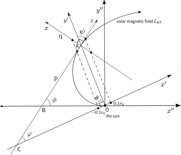
Figure 1: Schematic diagram of magnetic coordinate system $x-y-z$, solar coordinate systems $x^{\prime}-y’-z’$ and $x^{\prime\prime}-y^{\prime\prime}-z^{\prime\prime}$, the polar coordinate system, which are in ecliptic plane, and $z^{\prime}\parallel z^{\prime\prime}$.

In order to investigate the relative importance of the solar wind effect on along-field diffusion, it is necessary to derive the specific form of the solar wind effect, $\zeta$. Due to the magnetic freezing effect of plasmas and the solar rotation, the mean magnetic field of the sun presents a spiral form, which is called the Parker spiral. For simplicity, we consider it in the ecliptic plane. As shown in Figure 1, we consider a point $A$ with the solar magnetic field line $\mathcal{L}_{\mathrm{MF}}$ going through it. We set a coordinate system $x^{\prime}-y^{\prime}-z^{\prime}$, with the $y^{\prime}$-axis pointing from the sun to point $A$, the $z^{\prime}$-axis perpendicular to the ecliptic plane pointing towards the north, the $x^{\prime}$-axis defined using the right-hand rule, and the origin $O$ located at the center of the sun. We also set a polar coordinate system $r-\theta$, with the polar axis $r$ tangent to $\mathcal{L}_{\mathrm{MF}}$ at point $O$, the polar angle $\theta$ defined in a clockwise direction. In addition, another coordinate system $x^{\prime\prime}-y’^{\prime}-z^{\prime\prime}$ is established by rotating $x^{\prime}-y^{\prime}-z^{\prime}$ system with $\pi/2-\theta_{A}$ clockwise through point $O$, where $\theta_{A}$ is the polar angle of point $A$. Additionly, we set a magnetic coordinate system $x-y-z$, with the $z$-axis along the tangent of magnetic field line towards its positive direction, the $y$-axis parallel to $z^{\prime}$, and the $x$-axis satisfying right-hand rule. Moreover, the tangent of $\mathcal{L}_{\mathrm{MF}}$ at point $A$ is the straight line $y^{\prime}=kx^{\prime}+r_{0}$ with the intercept $r_{0}$, i.e., the distance from $O$ to $A$. We suppose the straight line can be written as $y^{\prime\prime}=k^{\prime}x^{\prime\prime}+l$ in $x^{\prime\prime}-y^{\prime\prime}-z^{\prime\prime}$ system. Furthermore, normal equation of $\mathcal{L}_{\mathrm{MF}}$ at point $A$ is $y^{\prime}=-x^{\prime}/k+r_{0}$.

Additionly, the angle between $z$-axis and $y^{\prime}$-axis is denoted as $\psi$. Therefore, the component of solar wind speed along solar magnetic field can be expressed as

$$V_{z}=V\cos\psi,$$ (46)

where $V$ is the magnitude of the solar wind velocity $\bm{V}$. It is obvious that the angle $\psi$ varies depending on the point on the magnetic field, and obeys the following formula on the ecliptic plane (e.g., Qin & Wu, 2021)

$$\cos\psi=\left(1+\frac{\omega^{2}r^{2}}{V^{2}}\right)^{-1/2}.$$ (47)

Here, $\omega$ is the angular velocity of the sun, and $r$ is the radial distance from the center of the sun to the point on solar magentic field. Thus, the influence $\zeta$ of the solar wind can be written as

$$\zeta=\int_{z_{1}}^{z_{2}}\mathrm{d}zF(z,t)V\left(1+\frac{\omega^{2}r^{2}}{V^{2}}\right)^{-1/2}-\int_{z_{1}}^{z_{2}}\mathrm{d}zzF(z,t)\int_{z_{1}}^{z_{2}}\mathrm{d}zF(z,t)V\left(1+\frac{\omega^{2}r^{2}}{V^{2}}\right)^{-1/2},$$ (48)

where $z_{1}$ and $z_{2}$ are the integral lower and upper limits, respectively. The integrals in Equation (48) are along the curve of the mean magnetic field, and the normalization condition needs to be satisfied

$$\int_{z_{1}}^{z_{2}}\mathrm{d}F(z,t)=1.$$ (49)

4.2 Exploring the relative importance of solar wind effect to along-field diffusion

In this paper, for the sake of simplicity, we assume that the speed $V$ of the solar wind is constant. Thus, Equation (48) can be written as

$$\zeta=V\int_{z_{1}}^{z_{2}}\mathrm{d}zzF(z,t)\left(1+\frac{\omega^{2}r^{2}}{V^{2}}\right)^{-1/2}-V\int_{z_{1}}^{z_{2}}\mathrm{d}zzF(z,t)\int_{z_{1}}^{z_{2}}\mathrm{d}zF(z,t)\left(1+\frac{\omega^{2}r^{2}}{V^{2}}\right)^{-1/2}.$$ (50)

In coodinate system $x^{\prime}-y^{\prime}-z^{\prime}$, if integral interval is small enought, the straight line $y^{\prime}=kx^{\prime}+r_{0}$ with $k=\tan\beta=\cot\psi$ can be used to approxmiately replace the curve of magnetic field line for the integrals in Equation (50), and the distribution function $F(x^{\prime},t)$ can be used to replace $F(z,t)$. Accordingly, as shown in Figure 1, the distance from $O$ to any point, $(x^{\prime},y^{\prime})$, between the integral interval $[z_{1},z_{2}]$ can be expressed as $r=\sqrt{x^{\prime 2}+(kx^{\prime}+r_{0})^{2}}$. In addition, we can obtain the formulas $\mathrm{d}z=\sqrt{1+(\mathrm{d}y^{\prime}/\mathrm{d}x^{\prime})^{2}}\mathrm{d}x^{\prime}$ and $z\approx\sqrt{1+(\mathrm{d}y^{\prime}/\mathrm{d}x^{\prime})^{2}}x^{\prime}$. To proceed, if the integral interval $[z_{1},z_{2}]$ is set as $[-0.1r_{0},0.1r_{0}]$ in coordinate system $x^{\prime}-y^{\prime}-z^{\prime}$, with the above setting, Equation (51) becomes

$$\zeta= V\left(1+k^{2}\right)\int_{-0.1r_{0}}^{0.1r_{0}}\mathrm{d}x^{\prime}x^{\prime}F(x^{\prime},t)\left(1+\frac{\omega^{2}\left[x^{\prime 2}+(kx^{\prime}+r_{0})^{2}\right]}{V^{2}}\right)^{-\frac{1}{2}}$$ (51)

$$-V\left(1+k^{2}\right)^{3/2}\int_{-0.1r_{0}}^{0.1r_{0}}\mathrm{d}x^{\prime}x^{\prime}F(x^{\prime},t)\int_{-0.1r_{0}}^{0.1r_{0}}\mathrm{d}x^{\prime}F(x^{\prime},t)\left(1+\frac{\omega^{2}\left[x^{\prime 2}+(kx^{\prime}+r_{0})^{2}\right]}{V^{2}}\right)^{-\frac{1}{2}}.$$

For mathematical tractability, in this article, we only explore the tail of SEPs, for which the distribution function $F(x^{\prime},t)$ is approximately uniform and is also approximately an even function of variable $x^{\prime}$ in integral interval $[-0.1r_{0},0.1r_{0}]$. Thus, the second term on the right-hand side of Equation (51) is equal to zero, and we have

$$\zeta= V\left(1+k^{2}\right)\int_{-0.1r_{0}}^{0.1r_{0}}\mathrm{d}x^{\prime}x^{\prime}F(x^{\prime},t)\left(1+\frac{\omega^{2}\left[x^{\prime 2}+(kx^{\prime}+r_{0})^{2}\right]}{V^{2}}\right)^{-\frac{1}{2}}.$$ (52)

In fact, based on the characterisitcs of each SEP events, the integral interval can also be set to other values. In this paper, we only qualitatively explore the solar wind effect on energetic particle along-field diffusion. Therefore, the interval length in Equation (52) does not affect the findings obtained in this paper.

With the integral interval $[-0.1r_{0},0.1r_{0}]$ and Equation (49), the normalization condition becomes

$$F(x^{\prime},t)=\frac{5}{r_{0}}.$$ (53)

Accordingly, the background solar wind effect on along-field diffusion can be written as

$$\zeta=\left(1+k^{2}\right)\frac{5V}{r_{0}}\int_{-0.1r_{0}}^{0.1r_{0}}\mathrm{d}x^{\prime}x^{\prime}\left(1+\frac{\omega^{2}\left[x^{\prime 2}+(kx^{\prime}+r_{0})^{2}\right]}{V^{2}}\right)^{-\frac{1}{2}}.$$ (54)

With integration by parts and a lengthy mathematical performance, the latter formula becomes

$$\zeta= \frac{2k\frac{V^{2}}{\omega}}{\sqrt{\left(0.1+\frac{1}{1+k^{2}}k\right)^{2}\left(1+k^{2}\right)+\frac{1}{\left(1+k^{2}\right)}+\frac{V^{2}}{\omega^{2}r_{0}^{2}}}+\sqrt{\left(-0.1+\frac{1}{1+k^{2}}k\right)^{2}\left(1+k^{2}\right)+\frac{1}{\left(1+k^{2}\right)}+\frac{V^{2}}{\omega^{2}r_{0}^{2}}}}$$ (55)

$$-\frac{5k}{\sqrt{1+k^{2}}}\frac{V^{2}}{\omega}\ln\frac{\left(0.1+\frac{1}{1+k^{2}}k\right)\sqrt{1+k^{2}}+\sqrt{\left(0.1+\frac{1}{1+k^{2}}k\right)^{2}\left(1+k^{2}\right)+\frac{1}{\left(1+k^{2}\right)}+\frac{V^{2}}{\omega^{2}r_{0}^{2}}}}{\left(-0.1+\frac{1}{1+k^{2}}k\right)\sqrt{1+k^{2}}+\sqrt{\left(-0.1+\frac{1}{1+k^{2}}k\right)^{2}\left(1+k^{2}\right)+\frac{1}{\left(1+k^{2}\right)}+\frac{V^{2}}{\omega^{2}r_{0}^{2}}}}.$$

Obviously, the latter equation contains the following two dimensionless quantities

$$\alpha_{1}\equiv\frac{V}{\omega r_{0}},$$ (56)

$$\alpha_{2}\equiv|k|.$$ (57)

For different limits of $\alpha_{1}$ and $\alpha_{2}$, the relative importance of the solar wind effect on along-field diffusion, $\zeta$, can be discussed. The results are summarized in Table 1.

4.2.1 The condition $\alpha_{1}\gg\alpha_{2}\gg 1$

Here, we suppose

$$\alpha_{1}\gg\alpha_{2}\gg 1,$$ (58)

which contains the inequalities

$$\alpha_{1}\gg\alpha_{2},$$ (59)

$$\alpha_{1}\gg 1,$$ (60)

$$\alpha_{2}\gg 1.$$ (61)

For the condition (58), Equation (55) is simplified as

$$\zeta=|k|Vr_{0}.$$ (62)

It is known that particle diffusion coefficient $\kappa_{zz}$ can be written as

$$\kappa_{zz}=\frac{u\lambda}{3},$$ (63)

where $\lambda$ is the mean free path of particles. With Equations (62) and (63), the relative importance of solar wind effect, $\zeta$, on the along-field diffusion is shown as follows

$$\frac{\zeta}{\kappa_{zz}}=3|k|\frac{Vr_{0}}{u\lambda}.$$ (64)

It is obvious that the following dimensionless quantity

$$\beta_{1}=|k|\frac{Vr_{0}}{u\lambda}$$ (65)

determines the relative importance of $\zeta$ to $\kappa_{zz}$. If $\beta_{1}\gtrsim 1$, the influence of solar wind effect, $\zeta$, on the along-field diffusion should be taken into account, conversely, if $\beta_{1}\ll 1$, $\zeta$ can be ignored. For the typical values of $V$, $u$, and $\lambda$ in Section 3, the dimensionless quantity becomes

$$\beta_{1}=|k|r_{0}\frac{V}{u\lambda}\sim 10|k|r_{0}.$$ (66)

Thus, we only need to explore the value of $kr_{0}$. The solar magnetic field can be described by

$$r_{0}=\frac{V}{\omega}\theta$$ (67)

with solar wind speed $V$ and solar rotation speed $\omega$. It is known that the angle $\theta$ of polar system inscreases in an clockwise direction. The parametric formulas of Equation (67) in coordinate system $x^{\prime\prime}-y^{\prime\prime}-z^{\prime\prime}$ are shown as

$$x^{\prime\prime}=\frac{V}{\omega}\theta\cos\theta,$$ (68)

$$y^{\prime\prime}=\frac{V}{\omega}\theta\sin\theta.$$ (69)

The slope of the tangent line at the point $A$ is $k^{\prime}=\tan\phi$ with the angle $\phi$ between $x^{\prime\prime}$-axis and the tangent. With the latter equations, the tangent slope of point $A$ on the magnetic field line in coordinate system $x^{\prime\prime}-y^{\prime\prime}-z^{\prime\prime}$ can be written as

$$k^{\prime}=\tan\phi=\frac{\mathrm{d}y^{\prime\prime}}{\mathrm{d}x^{\prime\prime}}=\frac{\mathrm{d}y^{\prime\prime}/\mathrm{d}\theta}{\mathrm{d}x^{\prime\prime}/\mathrm{d}\theta}=\frac{\theta+\tan\theta}{1-\theta\tan\theta}.$$ (70)

Similarly, the slope $k$ of the tangent is $k=\tan\varphi$ in coordinate system $x^{\prime}-y^{\prime}-z^{\prime}$, which satisfies

$$k=\tan\varphi=\tan\left(\phi+\theta-\frac{\pi}{2}\right)=\frac{2\theta\tan\theta+\tan^{2}\theta-1}{\theta+2\tan\theta-\theta\tan^{2}\theta}.$$ (71)

It is easily proved that slope $k$ is the generally increasing function of variable $\theta$. It is suggested that the points with $\theta=n\pi+\pi/2$ for integer numbers $n$ in Equation (71) are removable singularities, which do not affect the monotonicity of function $k$ with $\theta$. Therefore, the quantity $k$ is an appropriate parameter to reflect the influence of solar wind on particle transport, $\zeta$, at different spatial locations within the heliosphere. Accordingly, Equation (71) becomes

$$|k|r_{0}=\frac{V}{\omega}\theta\left|\frac{2\theta\tan\theta+\tan^{2}\theta-1}{\theta+2\tan\theta-\theta\tan^{2}\theta}\right|.$$ (72)

If $\theta\to 0$, for typical parameter values $V$ and $\omega$ listed above, we can obtain

$$|k|r_{0}\to 10^{10}\mathrm{m}.$$ (73)

Therefore, with Equation (66), we can find

$$\beta_{1}\sim 10|k|r_{0}\sim 10^{11}\gg 1.$$ (74)

In addition, Inequality (60) denotes $r_{0}\ll V/\omega\sim 10^{11}\mathrm{m}\sim 1$ AU, which indicates that the point $A$ is located in the inner heliosphere and Inequality (61). It is noted that Inequality (61), is consistent with the condition, Inequality (58). However, Inequality (58) leads to the relation $\alpha_{1}/\alpha_{2}\gg 1$, i.e., $|k|r_{0}\ll V/\omega$, which is contradictory to Equation (72) in the inner heliosphere. Therefore, for this case, the influence of solar wind on the along-field diffusion, $\zeta$, may not be taken into account.

4.2.2 The condition $\alpha_{2}\gg\alpha_{1}\gg 1$

In this subsection, we suppose

$$\alpha_{2}\gg\alpha_{1}\gg 1,$$ (75)

which contains

$$\alpha_{2}\gg\alpha_{1},$$ (76)

$$\alpha_{2}\gg 1,$$ (77)

$$\alpha_{1}\gg 1.$$ (78)

Equation (55) becomes

$$\zeta=-10\frac{V^{2}}{\omega}\ln\frac{\alpha_{2}}{\alpha_{1}}.$$ (79)

With the along-field diffusion coefficient formula, i.e., Equation (63), we find

$$\frac{\zeta}{\kappa_{zz}}=-30\frac{V^{2}}{u\omega\lambda}\ln\frac{\alpha_{2}}{\alpha_{1}}.$$ (80)

Obviously, the latter equation is determined by the following two dimensionless quantities

$$\beta_{2}=\frac{V^{2}}{u\omega\lambda},$$ (81)

$$\beta_{3}=\frac{\alpha_{2}}{\alpha_{1}}=\frac{\omega r_{0}|k|}{V}.$$ (82)

As shown in subsection 4.2.1, the condition $\alpha_{1}\gg 1$ and $\alpha_{2}\gg 1$ can only be satisfied in the inner heliosphere. However, from Inequality (76) we can obtain $\alpha_{2}/\alpha_{1}=\beta_{3}\gg 1$. For typical parameter values $V$ and $\omega$ in subsection 4.2.1, we find

$$|k|r_{0}\gg\frac{V}{\omega},$$ (83)

which cannot be satisfied in the inner heliosphere. Therefore, in this condition, the solar wind effect on along-field diffusion of energetic particles, $\zeta$, might be ignored.

4.2.3 The condition $\alpha_{1}\sim\alpha_{2}\gg 1$

In the following, we suppose

$$\alpha_{1}\sim\alpha_{2}\gg 1,$$ (84)

which contains two conditions

$$\alpha_{1}\sim\alpha_{2},$$ (85)

$$\alpha_{1}\gg 1,$$ (86)

$$\alpha_{2}\gg 1.$$ (87)

The condition (86) denotes $|k|r_{0}\sim V/\omega$, which is consistent with Equation (72) at least in the inner heliosphere. In addition, Inequality (86) corresponds to $r_{0}\ll V/\omega\sim 10^{11}m$, which indicates the point $A$ is located in the inner heliosphere. Inequality (87) also shows that the point $A$ is close to the sun.

Additionly, for the condition (84), Equation (55) is simplified as

$$\zeta=0.4\frac{V^{2}}{\omega}.$$ (88)

The ratio of $A$ to $\kappa_{zz}$ is

$$\frac{\zeta}{\kappa_{zz}}=1.2\frac{V^{2}}{u\omega\lambda},$$ (89)

which shows that the following dimensionless quantity determines the relative importance of solar wind effect

$$\beta_{2}=\frac{V^{2}}{u\omega\lambda}.$$ (90)

When $\beta_{2}\sim 1$, the solar wind effect on along-field diffusion of energetic particles, $\zeta$, is important. For the typical parameter values $V$, $\omega$, $u$, and $\lambda$ listed in subsection 4.2.1, we can obtain $\beta_{2}=0.3$. In summary, for Inequality (84), i.e., the point $A$ located in the inner heliosphere, solar wind effect on along-field diffusion, $\zeta$, is relatively important, so it should be considered.

4.2.4 The condition $\alpha_{1}\gg 1$ and $\alpha_{2}\ll 1$

Here, we suppose

$$\alpha_{1}\gg 1,$$ (91)

and

$$\alpha_{2}\ll 1.$$ (92)

For Inequalities (91) and (92), Equation (55) is simplified as

$$\zeta=|k|Vr_{0},$$ (93)

which is identical to Equation (62). Accordingly, the dimensionless quantity controlling the relative importance is

$$\beta_{1}=|k|\frac{Vr_{0}}{u\lambda}.$$ (94)

In addition, Inequality (91), i.e., $r_{0}\ll V/\omega$, corresponds to $r_{0}\ll 10^{11}m$, which denotes that the point $A$ is in the inner heliosphere. However, Inequality (92) represents that the slope of tangent line is very small, which indicates that the point $A$ is located in the outer heliosphere. Thus, the two Inequalities (91) and (92) are mutually contraditory. Therefore, for this case, the solar wind effect, $\zeta$, might not be considered.

4.2.5 The condition $\alpha_{2}\gg 1$ and $\alpha_{1}\ll 1$

In this subsection, we suppose the two inequalities

$$\alpha_{2}\gg 1,$$ (95)

$$\alpha_{1}\ll 1.$$ (96)

Using the the latter two inequalities, from Equation (55) we can obtain

$$\zeta=10\frac{V^{2}}{\omega}.$$ (97)

Comparing the latter formula with $\kappa_{zz}$, we can find the following dimensionless quantities

$$\beta_{2}=\frac{V^{2}}{u\omega\lambda}.$$ (98)

Inequality (95) indicates the point $A$ is in the inner heliosphere. Additionly, for the typical parameter values listed in Section 3, Inequality (96) denotes $r_{0}\gg 10^{11}$ m $\sim 1$ AU which indicates that the point $A$ is located in the outer heliosphere. Thus, Inequatity (95) is contradictory with Inequality (96). Therefore, for this case the solar wind effect, $\zeta$, on energetic particle transport may not be considered.

4.2.6 The condition $\alpha_{1}\ll 1$ and $\alpha_{2}\ll 1$

Now, we suppose the two inequalities

$$\alpha_{1}\ll 1,$$ (99)

$$\alpha_{2}\ll 1.$$ (100)

For the typical parameter values listed in Subsection 4.2.1, Inequality (99) gives $r_{0}\gg 10^{11}m$, which indicates the point $A$ located in the outer heliosphere. This is consistent with Inequality (100).

In addition, for the two Inequalitites (99) and (100), Equation (55) becomes

$$\zeta=|k|\frac{V^{2}}{\omega}.$$ (101)

By comparing the latter formula with $\kappa_{zz}$, we obtain

$$\frac{\zeta}{\kappa_{zz}}=3\frac{|k|V^{2}}{u\omega\lambda},$$ (102)

which is determined by the dimensionless quantities

$$\beta_{4}=\frac{|k|V^{2}}{u\omega\lambda}.$$ (103)

For the parameter values $V$, $u$, $\omega$, and $\lambda$ listed in Section 3, from Equation (103) we can obtain $|k|\geq 3$, which is contradictory to Inequality (100). Therefore, when energetic particle transport in the outer helioshere, the solar wind effect, $\zeta$, might not be taken into account.

4.3 Relative importance of the solar wind and adiabatic focusing effects

The second term on the right-hand side of Equation (29) was evaluated by Wang & Qin (2018, 2019) as

$$T_{2}=\kappa_{z}\kappa_{tz}\approx\frac{14}{135}\frac{u\lambda^{3}}{L^{2}}.$$ (104)

Acccordingly, the ratio of adiabatic focusing effect term $T_{2}$ to along-field Fick’s law diffusion term $T_{1}$ is

$$\frac{T_{2}}{T_{1}}=\frac{\kappa_{z}\kappa_{tz}}{\kappa_{zz}}\approx 0.3\xi^{2}.$$ (105)

with the dimensionless quantity

$$\xi=\frac{\lambda}{L}.$$ (106)

Here, $\lambda$ is the mean free path of charged energetic particles and $L$ is the characteristic length of adiabatic focusing. Obviously, the dimensionless quantity $\xi$ determines the relative importance of $T_{2}$ to $T_{1}$. From Equations (105) and (106), we can find that if $\xi\gtrsim 1$, adiabatic focusing effect need to be taken into account. If $\xi\ll 1$, the adiabatic focusing effect should be ignored.

In Subsection 4.2, the influence of solar wind on along-field diffusion is explored. In the condition with strong solar wind effect, $\alpha_{1}\sim\alpha_{2}\gg 1$, considering the formulas of the solar wind effect $T_{3}$ and adiabatic focusing effect $T_{2}$, we have

$$\frac{T_{3}}{T_{2}}=\frac{27}{7}\frac{V^{2}L^{2}}{u\omega\lambda^{3}}.$$ (107)

Obviously, the following dimensionless quantity can be found

$$\gamma=\frac{V^{2}L^{2}}{u\omega\lambda^{3}}=\frac{V^{2}}{u\omega\lambda}\xi^{2}.$$ (108)

For typical parameter values in Section 3, thedimensionless quantity $\gamma\approx 0.3$. Thus, if $\xi\sim 1$ is satisfied, both the solar wind effect and the adiabatic focusing effect should be considered.

5 The influence of solar wind effect on cross-field diffusion

Next, based on Equation (43), we investigate the solar wind effect on eneregtic particle cross-field diffusion.

5.1 The integrating form of the solar wind effect, $\eta$

From Equation (43), the solar wind effect on the cross-field diffusion can be written as

$$\eta=\int_{-x_{0}}^{x_{0}}\mathrm{d}xxV_{x}F_{b}-\int_{-x_{0}}^{x_{0}}\mathrm{d}xxF_{b}\int_{-x_{0}}^{x_{0}}\mathrm{d}xV_{x}F_{b}$$ (109)

From Figure 1, the following formula can be found

$$V_{\perp}=V\sin\psi.$$ (110)

In this article, for the sake of simplicity, we assume that $V_{\perp}\sim V_{x}$ and the solar wind speed $V$ is constant. Thus, Equation (109) becomes

$$\eta=V\int_{-x_{0}}^{x_{0}}\mathrm{d}xxF_{b}\sin\psi-V\int_{-x_{0}}^{x_{0}}\mathrm{d}xxF_{b}\int_{-x_{0}}^{x_{0}}\mathrm{d}xF_{b}\sin\psi.$$ (111)

Obviously, the angle $\psi$ varies depending on the point $A$ and obeys the following formula on the ecliptic plane (e.g., Qin & Wu, 2021)

$$\sin\psi=\frac{\omega r}{V}\left(\frac{\omega^{2}r^{2}}{V^{2}}+1\right)^{-\frac{1}{2}}.$$ (112)

Inserting the latter formula into Equation (111), we have

$$\eta=V\int_{-x_{0}}^{x_{0}}\mathrm{d}xxF_{b}\frac{\omega r}{V}\left(\frac{\omega^{2}r^{2}}{V^{2}}+1\right)^{-\frac{1}{2}}-V\int_{-x_{0}}^{x_{0}}\mathrm{d}xxF_{b}\int_{-x_{0}}^{x_{0}}\mathrm{d}xF_{b}\frac{\omega r}{V}\left(\frac{\omega^{2}r^{2}}{V^{2}}+1\right)^{-\frac{1}{2}}.$$ (113)

To proceed, for simplicity, we assume that the distribution function $F_{b}$ is approximately constant. Thus, the formula $\int_{-x_{0}}^{x_{0}}\mathrm{d}xxF_{b}=0$ holds, and Equation (113) becomes

$$\eta=V\int_{-x_{0}}^{x_{0}}\mathrm{d}xxF_{b}\frac{\omega r}{V}\left(\frac{\omega^{2}r^{2}}{V^{2}}+1\right)^{-\frac{1}{2}}.$$ (114)

From the equation of normal line, $y^{\prime}=-x^{\prime}/k+r_{0}$, we can obtain the formulas $\mathrm{d}x=\sqrt{1+(\mathrm{d}y^{\prime}/\mathrm{d}x^{\prime})^{2}}\mathrm{d}x^{\prime}=\sqrt{1+1/k^{2}}\mathrm{d}x^{\prime}$ and $x=\sqrt{1+(\mathrm{d}^{\prime}y/\mathrm{d}x^{\prime})^{2}}x^{\prime}=\sqrt{1+1/k^{2}}x^{\prime}$, Equation (114) becomes

$$\eta=V\left(1+\frac{1}{k^{2}}\right)\int_{-0.1r_{0}}^{0.1r_{0}}\mathrm{d}x^{\prime}x^{\prime}F_{b}\frac{\omega r}{V}\left(\frac{\omega^{2}r^{2}}{V^{2}}+1\right)^{-\frac{1}{2}},$$ (115)

where we set $x_{0}=0.1r_{0}/\cos\psi$. Thus, from the normalization condition $\int_{-0.1r_{0}}^{0.1r_{0}}\mathrm{d}x^{\prime}F_{b}=1$, we can find

$$F_{b}=\frac{5}{r_{0}}.$$ (116)

Accordingly, Equation (115) becomes

$$\eta=V\frac{5}{r_{0}}\left(1+\frac{1}{k^{2}}\right)\int_{-0.1r_{0}}^{0.1r_{0}}\mathrm{d}x^{\prime}x^{\prime}\frac{\omega r}{V}\left(\frac{\omega^{2}r^{2}}{V^{2}}+1\right)^{-\frac{1}{2}}.$$ (117)

Using the dimensionless quantity $\alpha_{1}=V/(\omega r_{0})$, we can rewrite Equation (115) as

$$\eta=V\frac{5}{r_{0}}\left(1+\frac{1}{k^{2}}\right)\int_{-0.1r_{0}}^{0.1r_{0}}\mathrm{d}x^{\prime}x^{\prime}\left(\alpha_{1}^{2}\frac{r_{0}^{2}}{r^{2}}+1\right)^{-\frac{1}{2}}.$$ (118)

The latter equation is very complex, so it is not easy to be evaluated. However, the relation $r_{0}/r\sim 1$ approximately holds because the integral interval is small enough, so that Equation (118) can be qualitatively explored for $\alpha_{1}\gg 1$ and $\alpha_{1}\ll 1$.

5.2 The condition $\alpha_{1}\gg 1$

For $\alpha_{1}\gg 1$, with $r=\sqrt{x^{\prime 2}+\left(-x^{\prime}/k+r_{0}\right)^{2}}$, Equation (118) is simplified as

$$\eta=10\frac{\omega}{r_{0}}\frac{1+k^{2}}{k^{2}}\int_{0}^{0.1r_{0}}\mathrm{d}x^{\prime}x^{\prime}\sqrt{x^{\prime 2}+\left(-x^{\prime}/k+r_{0}\right)^{2}}.$$ (119)

After a lengthy mathematical performance, the latter equation becomes

$$\eta=\frac{10}{3}\omega r_{0}^{2}\frac{\left(1+k^{2}\right)^{3/2}}{k^{3}}\Bigg{\{}\left[\left(0.1-\frac{k}{1+k^{2}}\right)^{2}+\frac{k^{4}}{\left(1+k^{2}\right)^{2}}\right]^{3/2}-\left[\frac{k^{2}}{\left(1+k^{2}\right)^{2}}+\frac{k^{4}}{\left(1+k^{2}\right)^{2}}\right]^{3/2}\Bigg{\}}.$$ (120)

In the following, we evaluate the solar wind effect on cross-field diffusion, $\eta$, for $\alpha_{2}=|k|\to\infty$ and $\alpha_{2}=|k|\to 0$, respectively.

5.2.1 The condition $\alpha_{2}=|k|\to\infty$

For the condition

$$\alpha_{2}=|k|\to\infty,$$ (121)

we can easily obtain

$$\eta\approx 1.5\omega r_{0}^{2}.$$ (122)

Comparing the latter formula with $\kappa_{xx}=u\lambda_{\perp}/3$ we obtain

$$\frac{\eta}{\kappa_{xx}}=4.5\frac{\omega r_{0}^{2}}{u\lambda_{\perp}}\sim\frac{\omega r_{0}^{2}}{u\lambda_{\perp}}.$$ (123)

Obviously, the following dimensionless quantity determines the relative importance of solar wind effect on cross-field diffusion

$$\delta_{1}=\frac{\omega r_{0}^{2}}{u\lambda_{\perp}}.$$ (124)

In the condition (121), the point $A$ should be close to the sun. Thus, the distance $r_{0}$ is much less than 1 AU, i.e., $r_{0}\ll 10^{11}$ m. In addition, for the typical parameter values $\omega$, $u$, and $\lambda_{\perp}$ in Section 3, we have

$$\delta_{1}\ll 1,$$ (125)

which indicates the solar wind effect on the along-field diffusion, $\eta$, may be ignored.

5.2.2 The condition $\alpha_{2}\to 0$

For $\alpha_{2}\to 0$, we can obtain

$$\eta\approx 0.1\frac{\omega r_{0}^{2}}{k^{3}}.$$ (126)

Comparing the term $\eta$ and the cross-field diffusion coefficient $\kappa_{xx}$ yields

$$\frac{\eta}{\kappa_{xx}}=0.3\frac{\omega r_{0}^{2}}{u\lambda_{\perp}k^{3}}.$$ (127)

It is obvious that the following dimensionless quantity determines the relative importance of solar wind to cross-field diffusion

$$\delta_{2}=\frac{\omega r_{0}^{2}}{u\lambda_{\perp}k^{3}}.$$ (128)

For the typical parameter values $u$, $\omega$, $\lambda_{\perp}$ in Section 3, we can obtain

$$\delta_{2}\sim\left(10^{-11}r_{0}\right)^{2}\frac{1}{k^{3}}.$$ (129)

For $\delta_{2}\geq 1$, the relation $k\leq\left(10^{-11}r_{0}\right)^{2/3}$ holds. However, the condition $\alpha_{1}\gg 1$ corresponds to $r_{0}\ll V/\omega\sim 10^{11}$ m, which denotes that the point $A$ is in the inner heliosphere. The condition $\alpha_{1}\gg 1$ is contradictory to $\alpha_{2}\to 0$ which indicates the point $A$ in the outer heliosphere. Therefore, the solar wind effect on cross-field diffusion, $\eta$, may be ignored.

5.3 The condition $\alpha_{1}\ll 1$

If $\alpha_{1}\ll 1$, with $\int_{-0.1r_{0}}^{0.1r_{0}}\mathrm{d}xF_{b}=1$, Equation (113) becomes

$$\eta= V\int_{-0.1r_{0}}^{0.1r_{0}}\mathrm{d}xxF_{b}-V\int_{-0.1r_{0}}^{0.1r_{0}}\mathrm{d}xxF_{b}=0.$$ (130)

Obviously, for this case, the solar wind effect, $\eta$, might not be taken into account.

6 SUMMARY AND CONCLUSION

In this paper, starting from the focusing equation, we derive the formulas of the mean square displacement definitions of along- and cross-field diffusion coefficients, $\kappa_{zz}^{DV}$ and $\kappa_{xx}^{DV}$, respectively. It is demonstrated that $\kappa_{zz}^{DV}$ includes solar wind effect, i.e., $\zeta=\left\langle zV_{z}\right\rangle-\left\langle z\right\rangle\left\langle V_{z}\right\rangle$, and $\kappa_{xx}^{DV}$ contains $\eta=\left\langle xV_{x}\right\rangle-\langle x\rangle\langle V_{x}\rangle$.

For different limits of dimensionless quantities $\alpha_{1}=V/(\omega r_{0})$ and $\alpha_{2}=|k|$, the relative importance of the solar wind effect on along-field diffusion, $\zeta$, is expored, and corresponding dimensionless quantities are obtained, which are summarized in Table 1. For the condition $\alpha_{1}\sim\alpha_{2}\gg 1$, we find that when the point $A$ is close to the sun, the relative importance of solar wind effect on along-field diffusion, $\zeta$, should be taken into account. In this condition, we find that when $\xi=\lambda/L\geq 1$, the adiabatic focusing effects need also to be considered. Next, the relative importance of solar wind effect on cross-field diffusion, $\eta$, is investigated in several extreme conditions, we find that the solar wind effect on cross-field diffusion, $\eta$, might be ignored.

The results obtained in this paper have certain significance in the transport of energetic particles not only in the heliosphere, but also in many other scenarios, such as, planetary magnetoshere and ionoshere, intersteller space, the spaces close to neutron stars, supernova remanents and so on. It is possible that in some conditions, the solar wind effect on energetic particle diffusion in the heliosphere is not important, but the background plasma speed effect on energetic particle diffusion in other scenarios is not ignorable.

In this article, the results we get are not very conclusive. We only perform the exploration in some extreme conditions. In addition, we set some paramters with typical values as shown in Section 3, which are standard in $1$ AU for energetic particles. However, using the typical parameter values, we discuss solar wind effect on diffusion coefficients in some special conditions, e.g., $r_{0}\ll 1$ AU, in which the typical parameter values may be not appropriate in the condition. In the future, we will investigate solar wind effect on diffusion coefficients in more general conditions, using more reasonalble typical parameter values in special conditions.

Other physical effects, e.g., solar wind of spatial derivative, momentum transport, etc., on both spatial diffusion and drift coefficients, may also be investigated. In past decades, the non-diffusion, i.e., subdiffusion and superdiffusion, has gained more and more interest due to its general applications in numerous research field. We may also investigate the influence of the solar wind and adiabatic focusing on non-diffusion of energetic particles.

Appendix A The focusing equation satisfying particle number conservation law

The focusing equation, which has been broadly used to research charged particle transport, is as follow

$$\frac{\partial{f}}{\partial{t}}= \nabla\cdot\left(\kappa_{\perp}\cdot\nabla f\right)-\left(u\mu\hat{\bm{b}}+\bm{V}\right)\cdot\nabla f+\frac{\partial{}}{\partial{\mu}}\left(D_{\mu\mu}\frac{\partial{f}}{\partial{\mu}}\right)+\frac{dp}{dt}\frac{\partial{f}}{\partial{p}}+\frac{d\mu}{dt}\frac{\partial{f}}{\partial{\mu}}$$ (A-1)

with

$$\frac{dp}{dt}=p\Bigg{[}\frac{1-\mu^{2}}{2}\left(\nabla\cdot\bm{V}-\hat{\bm{b}}\hat{\bm{b}}:\nabla\bm{V}\right)+\mu^{2}\hat{\bm{b}}\hat{\bm{b}}:\nabla\bm{V}\Bigg{]},$$ (A-2)

$$\frac{d\mu}{dt}=\frac{1-\mu^{2}}{2}\Bigg{[}-\frac{u}{L}-\mu\left(\nabla\cdot\bm{V}-3\hat{\bm{b}}\hat{\bm{b}}:\nabla\bm{V}\right)\Bigg{]}.$$ (A-3)

Here, $L=\left(\hat{\bm{b}}\cdot\nabla\ln B\right)^{-1}$. However, this formulation does not satisfy particle number conservation law which is one of the most important physical laws. Therefore, we have to find a focusing equation which satisfies the particle number conservation law.

For spherical system $(p,\theta,\phi)$, the nabla operator of momentum space is

$$\nabla_{p}f=\frac{\partial{f}}{\partial{p}}\bm{e}_{p}+\frac{1}{p}\frac{\partial{f}}{\partial{\theta}}\bm{e}_{\theta}+\frac{1}{p\sin\theta}\frac{\partial{f}}{\partial{\phi}}\bm{e}_{\phi}.$$ (A-4)

In this paper, we only consider gyrotropic case, and Equation (A-4) becomes

$$\nabla_{p}f=\frac{\partial{f}}{\partial{p}}\bm{e}_{p}+\frac{1}{p}\frac{\partial{f}}{\partial{\theta}}\bm{e}_{\theta}.$$ (A-5)

Because $\mu=\cos\theta$, we have

$$\frac{\partial{}}{\partial{\theta}}=\frac{\partial{}}{\partial{\mu}}\frac{\partial{\mu}}{\partial{\theta}}=-\sin\theta\frac{\partial{}}{\partial{\mu}}.$$ (A-6)

Inserting the latter equation into Equation (A-5) gives

$$\nabla_{p}f=\frac{\partial{f}}{\partial{p}}\bm{e}_{p}-\sin\theta\frac{1}{p}\frac{\partial{f}}{\partial{\mu}}\bm{e}_{\theta}.$$ (A-7)

To proceed, we have

$$\bm{a}\cdot\nabla_{p}f=\left(a_{p}\bm{e}_{p}+a_{\theta}\bm{e}_{\theta}\right)\cdot\left(\frac{\partial{f}}{\partial{p}}\bm{e}_{p}-\frac{\sin\theta}{p}\frac{\partial{f}}{\partial{\mu}}\bm{e}_{\theta}\right)=a_{p}\frac{\partial{f}}{\partial{p}}-a_{\theta}\frac{\sin\theta}{p}\frac{\partial{f}}{\partial{\mu}}$$ (A-8)

With the following formula

$$\bm{a}\cdot\nabla_{p}f=\frac{dp}{dt}\frac{\partial{f}}{\partial{p}}+\frac{d\mu}{dt}\frac{\partial{f}}{\partial{\mu}},$$ (A-9)

we obtain

$$\frac{dp}{dt}=a_{p},$$ (A-10)

$$\frac{d\mu}{dt}=-a_{\theta}\frac{\sin\theta}{p}.$$ (A-11)

That is, the latter formulas can be rewritten as

$$a_{p}=\frac{dp}{dt},$$ (A-12)

$$a_{\theta}=-\frac{d\mu}{dt}\frac{p}{\sin\theta}.$$ (A-13)

Considering Equations (A-2) and (A-3), we can find that

$$a_{p}=p\Bigg{[}\frac{1-\mu^{2}}{2}\left(\nabla\cdot\bm{V}-\hat{\bm{b}}\hat{\bm{b}}:\nabla\bm{V}\right)+\mu^{2}\hat{\bm{b}}\hat{\bm{b}}:\nabla\bm{V}\Bigg{]},$$ (A-14)

$$a_{\theta}=\frac{p}{\sin\theta}\frac{1-\mu^{2}}{2}\Bigg{[}\frac{u}{L}+\mu\left(\nabla\cdot\bm{V}-3\hat{\bm{b}}\hat{\bm{b}}:\nabla\bm{V}\right)\Bigg{]}.$$ (A-15)

Inserting formulas (A-12) and (A-13) into the following equation

$$\nabla_{p}\cdot\left(\bm{a}f\right)= \frac{1}{p^{2}}\frac{\partial{}}{\partial{p}}\left(p^{2}a_{p}f\right)-\frac{1}{p}\frac{\partial{}}{\partial{\mu}}\left(\sin\theta a_{\theta}f\right),$$ (A-16)

we can obtain

$$\nabla_{p}\cdot\left(\bm{a}f\right)= \frac{1}{p^{2}}\frac{\partial{}}{\partial{p}}\Bigg{\{}p^{3}\Bigg{[}\frac{1-\mu^{2}}{2}\left(\nabla\cdot\bm{V}-\hat{\bm{b}}\hat{\bm{b}}:\nabla\bm{V}\right)+\mu^{2}\hat{\bm{b}}\hat{\bm{b}}:\nabla\bm{V}\Bigg{]}f\Bigg{\}}$$ (A-17)

$$+\frac{\partial{}}{\partial{\mu}}\Bigg{\{}\frac{1-\mu^{2}}{2}\Bigg{[}-\frac{u}{L}-\mu\left(\nabla\cdot\bm{V}-3\hat{\bm{b}}\hat{\bm{b}}:\nabla\bm{V}\right)\Bigg{]}f\Bigg{\}}.$$

The Fokker-Planck equation is shown as

$$\frac{\partial{f}}{\partial{t}}+\nabla\cdot\left(\bm{v}f\right)+\nabla_{p}\cdot\left(\bm{a}f\right)=\nabla\cdot\left(\kappa\cdot\nabla f\right)+\nabla_{p}\cdot\left(\kappa\cdot\nabla_{p}f\right),$$ (A-18)

which satisfies the particle number conservation law. By considering the latter formula and the following fomulas

$$\bm{v}=u\mu\hat{\bm{b}}+\bm{V},$$ (A-19)

$$\nabla\cdot\left(\kappa\cdot\nabla f\right)=\nabla\cdot\left(\kappa_{\perp}\cdot\nabla f\right),$$ (A-20)

$$\nabla_{p}\cdot\left(\kappa\cdot\nabla_{p}f\right)=\frac{\partial{}}{\partial{\mu}}\left(D_{\mu\mu}\frac{\partial{f}}{\partial{\mu}}\right),$$ (A-21)

Equation (A-18) becomes

$$\frac{\partial{f}}{\partial{t}}=\nabla\cdot\left(\kappa_{\perp}\cdot\nabla f\right)-\nabla\cdot\left[\left(u\mu\hat{\bm{b}}+\bm{V}\right)f\right]+\frac{\partial{}}{\partial{\mu}}\left(D_{\mu\mu}\frac{\partial{f}}{\partial{\mu}}\right)$$

$$+\frac{1}{p^{2}}\frac{\partial{}}{\partial{p}}\Bigg{\{}p^{3}\Bigg{[}\frac{1-\mu^{2}}{2}\left(\nabla\cdot\bm{V}-\hat{\bm{b}}\hat{\bm{b}}:\nabla\bm{V}\right)+\mu^{2}\hat{\bm{b}}\hat{\bm{b}}:\nabla\bm{V}\Bigg{]}f\Bigg{\}}$$

$$+\frac{\partial{}}{\partial{\mu}}\Bigg{\{}\frac{1-\mu^{2}}{2}\Bigg{[}-\frac{u}{L}-\mu\left(\nabla\cdot\bm{V}-3\hat{\bm{b}}\hat{\bm{b}}:\nabla\bm{V}\right)\Bigg{]}f\Bigg{\}},$$ (A-22)

which is our starting point of this paper.

In fact, if the incompressible condition

$$\nabla\cdot\bm{v}+\nabla_{p}\cdot\bm{a}=0$$ (A-23)

holds, Equation (A-1) can also satisfy particle number conservation. Now, the specific form of the incompressible condition is derived. With the divergence formula

$$\nabla\cdot\bm{A}=\frac{1}{r^{2}}\frac{\partial{}}{\partial{r}}\left(r^{2}f_{r}\right)+\frac{1}{r\sin\theta}\frac{\partial{}}{\partial{\theta}}\left(\sin\theta f_{\theta}\right)+\frac{1}{r\sin\theta}\frac{\partial{f_{\phi}}}{\partial{\phi}},$$ (A-24)

for gyrotropic case the latter formula becomes

$$\nabla\cdot\bm{A}=\frac{1}{r^{2}}\frac{\partial{}}{\partial{r}}\left(r^{2}f_{r}\right)+\frac{1}{r\sin\theta}\frac{\partial{}}{\partial{\theta}}\left(\sin\theta f_{\theta}\right)$$ (A-25)

Using $\mu=\cos\theta$, the latter formula can be rewritten as

$$\nabla\cdot\bm{A}=\frac{1}{r^{2}}\frac{\partial{}}{\partial{r}}\left(r^{2}f_{r}\right)-\frac{1}{r}\frac{\partial{}}{\partial{\mu}}\left(\sin\theta f_{\theta}\right).$$ (A-26)

In addition, the divergence formula for velocity is shown as

$$\nabla\cdot\bm{v}=\nabla\cdot\left(u\mu\hat{\bm{b}}+\bm{V}\right)=\nabla\cdot\bm{V}.$$ (A-27)

Similarly, with Equations (A-12) and (A-13), the divergence formula for acceleration can be obtained

$$\nabla_{p}\cdot\bm{a}= \frac{1}{p^{2}}\frac{\partial{}}{\partial{p}}\left(p^{2}a_{p}\right)-\frac{1}{p}\frac{\partial{}}{\partial{\mu}}\left(\sin\theta a_{\theta}\right)$$ (A-28)

$$=\frac{1}{p^{2}}\frac{\partial{}}{\partial{p}}\Bigg{\{}p^{3}\Bigg{[}\frac{1-\mu^{2}}{2}\left(\nabla\cdot\bm{V}-\hat{\bm{b}}\hat{\bm{b}}:\nabla\bm{V}\right)+\mu^{2}\hat{\bm{b}}\hat{\bm{b}}:\nabla\bm{V}\Bigg{]}\Bigg{\}}$$

$$-\frac{1}{p}\frac{\partial{}}{\partial{\mu}}\Bigg{\{}\sin\theta\frac{p}{\sin\theta}\frac{1-\mu^{2}}{2}\Bigg{[}\frac{u}{L}+\mu\left(\nabla\cdot\bm{V}-3\hat{\bm{b}}\hat{\bm{b}}:\nabla\bm{V}\right)\Bigg{]}\Bigg{\}}$$

To continue, the latter formula can be simplified as

$$\nabla_{p}\cdot\bm{a}=\nabla\cdot\bm{V}+\left(3\mu^{2}-1\right)\hat{\bm{b}}\hat{\bm{b}}:\nabla\bm{V}+\frac{u\mu}{L}.$$ (A-29)

Combining Equations (A-27) and (A-29) yields

$$\nabla\cdot\bm{v}+\nabla_{p}\cdot\bm{a}=2\nabla\cdot\bm{V}+\left(3\mu^{2}-1\right)\hat{\bm{b}}\hat{\bm{b}}:\nabla\bm{V}+\frac{u\mu}{L}=0$$ (A-30)

Thus, the condition of particle number conservation can be rewritten as

$$-\frac{u\mu}{L}=2\nabla\cdot\bm{V}+\left(3\mu^{2}-1\right)\hat{\bm{b}}\hat{\bm{b}}:\nabla\bm{V}$$ (A-31)

If the latter condition is satisfied, Equation (A-1) also satisfies the particle number conservation law.

Appendix B The focusing equation without tensor operation

For mathematical tractability, the focusing equation can be rewritten as

$$\frac{\partial{f}}{\partial{t}}=\nabla\cdot\left(\kappa_{\perp}\cdot\nabla f\right)-\nabla\cdot\left[\left(u\mu\hat{\bm{b}}+\bm{V}\right)f\right]+\frac{\partial{}}{\partial{\mu}}\left(D_{\mu\mu}\frac{\partial{f}}{\partial{\mu}}\right)$$

$$+\frac{1}{p^{2}}\frac{\partial{}}{\partial{p}}\Bigg{\{}p^{3}\Bigg{[}\frac{1-\mu^{2}}{2}\left(\frac{\partial{V_{x}}}{\partial{x}}+\frac{\partial{V_{y}}}{\partial{y}}\right)+\mu^{2}\frac{\partial{V_{z}}}{\partial{z}}\Bigg{]}f\Bigg{\}}$$

$$+\frac{\partial{}}{\partial{\mu}}\Bigg{\{}\frac{1-\mu^{2}}{2}\Bigg{[}-\frac{u}{L}-\mu\left(\frac{\partial{V_{x}}}{\partial{x}}+\frac{\partial{V_{y}}}{\partial{y}}-2\frac{\partial{V_{z}}}{\partial{z}}\right)\Bigg{]}f\Bigg{\}},$$ (B-1)

with the following formulas

$$\bm{V}^{SW}=V_{z}^{SW}\hat{\bm{b}}+V_{x}^{SW}\hat{\bm{n}_{x}}+V_{y}^{SW}\hat{\bm{n}_{y}},$$ (B-2)

$$\nabla=\frac{\partial}{\partial{z}}\hat{\bm{b}}+\frac{\partial}{\partial{x}}\hat{\bm{n}_{x}}+\frac{\partial}{\partial{y}}\hat{\bm{n}_{y}},$$ (B-3)

$$\hat{\bm{b}}\cdot\nabla=\hat{\bm{b}}\cdot\left(\frac{\partial}{\partial{z}}\hat{\bm{b}}+\frac{\partial}{\partial{x}}\hat{\bm{n}_{x}}+\frac{\partial}{\partial{y}}\hat{\bm{n}_{y}}\right)=\frac{\partial}{\partial{z}},$$ (B-4)

$$\nabla\cdot\hat{\bm{b}}=\left(\frac{\partial}{\partial{z}}\hat{\bm{b}}+\frac{\partial}{\partial{x}}\hat{\bm{n}_{x}}+\frac{\partial}{\partial{y}}\hat{\bm{n}_{y}}\right)\cdot\hat{\bm{b}}=\frac{\partial}{\partial{z}},$$ (B-5)

$$\hat{\bm{b}}\cdot\bm{V}^{SW}=\hat{\bm{b}}\cdot\left(V_{z}^{SW}\hat{\bm{b}}+V_{x}^{SW}\hat{\bm{n}_{x}}+V_{y}^{SW}\hat{\bm{n}_{y}}\right)=V_{z}^{SW},$$ (B-6)

$$\hat{\bm{b}}\hat{\bm{b}}:\nabla\bm{V}^{SW}=\left(\hat{\bm{b}}\cdot\nabla\right)\left(\hat{\bm{b}}\cdot\bm{V}^{SW}\right)=\frac{\partial{V_{z}^{SW}}}{\partial{z}},$$ (B-7)

$$\nabla\cdot\bm{V^{SW}}=\left(\frac{\partial}{\partial{z}}\hat{\bm{b}}+\frac{\partial}{\partial{x}}\hat{\bm{n}_{x}}+\frac{\partial}{\partial{y}}\hat{\bm{n}_{y}}\right)\left(V_{z}^{SW}\hat{\bm{b}}+V_{x}^{SW}\hat{\bm{n}_{x}}+V_{y}^{SW}\hat{\bm{n}_{y}}\right)=\frac{\partial{V_{z}^{SW}}}{\partial{z}}+\frac{\partial{V_{x}^{SW}}}{\partial{x}}+\frac{\partial{V_{y}^{SW}}}{\partial{y}},$$ (B-8)

$$\nabla\cdot\bm{V^{SW}}-\hat{\bm{b}}\hat{\bm{b}}:\nabla\bm{V}^{SW}=\frac{\partial{V_{x}^{SW}}}{\partial{x}}+\frac{\partial{V_{y}^{SW}}}{\partial{y}},$$ (B-9)

$$\nabla\cdot\left(\bm{V}^{SW}F\right)=\left(\frac{\partial}{\partial{z}}\hat{\bm{b}}+\frac{\partial}{\partial{x}}\hat{\bm{n}_{x}}+\frac{\partial}{\partial{y}}\hat{\bm{n}_{y}}\right)\left(V_{z}^{SW}F\hat{\bm{b}}+V_{x}^{SW}F\hat{\bm{n}_{x}}+V_{y}^{SW}F\hat{\bm{n}_{y}}\right)$$

$$=\frac{\partial{\left(V_{z}^{SW}F\right)}}{\partial{z}}+\frac{\partial{\left(V_{x}^{SW}F\right)}}{\partial{x}}+\frac{\partial{\left(V_{y}^{SW}F\right)}}{\partial{y}},$$ (B-10)

$$\nabla\cdot\bm{V^{SW}}-3\hat{\bm{b}}\hat{\bm{b}}:\nabla\bm{V}^{SW}=\frac{\partial{V_{x}^{SW}}}{\partial{x}}+\frac{\partial{V_{y}^{SW}}}{\partial{y}}-2\frac{\partial{V_{z}^{SW}}}{\partial{z}}.$$ (B-11)

Table 1: The dimensionless quantities determining the relative importance of solar wind effect on along-field diffusion

Range	solar wind effect
$\alpha_{1}\gg\alpha_{2}\gg 1$	$A=|k|Vr_{0}$	$\beta_{1}=\frac{|k|Vr_{0}}{u\lambda}$
$\alpha_{2}\gg\alpha_{1}\gg 1$	$A=-10\frac{V^{2}}{\omega}\ln\frac{\omega r_{0}|k|}{V}$	$\beta_{2}=\frac{V^{2}}{u\omega\lambda}$,
		$\beta_{3}=\frac{\omega r_{0}|k|}{V}$
$\alpha_{1}\sim\alpha_{2}\gg 1$	$A=0.4\frac{V^{2}}{\omega}$	$\beta_{2}=\frac{V^{2}}{u\omega\lambda}$
$\alpha_{1}\gg 1$, $\alpha_{2}\ll 1$	$A=|k|Vr_{0}$	$\beta_{1}=\frac{|k|Vr_{0}}{u\lambda}$
$\alpha_{2}\ll 1$, $\alpha_{1}\gg 1$	$A=10\frac{V^{2}}{\omega}$	$\beta_{2}=\frac{V^{2}}{u\omega\lambda}$
$\alpha_{1}\ll 1$, $\alpha_{2}\ll 1$	$A=|k|\frac{V^{2}}{\omega}$	$\beta_{4}=\frac{|k|V^{2}}{u\omega\lambda}$

References

• (1)
• (2)
• (3)
• Beeck & Wibberenz (1986) Beeck, J., & Wibberenz, G. 1986, ApJ, 311, 437
• Bian & Emslie (2020) Bian, N. H., & Emslie, A. G. 2020, ApJ, 897, 34
• Bieber & Burger (1990) Bieber, J. W., & Burger, R. A. 1990, ApJ, 348, 597
• Dröge et al. (2010) Dröge, W., Kartavykh, Y. Y., Klecker, B., & Kovaltsov, G. A. 2010, ApJ, 709, 912
• Duderstadt & Martin (1979) Duderstadt, J. J., & Martin, W. R. 1979, Transport theory, John Wiley & Sons
• Earl (1976) Earl, J. A. 1976, ApJ, 205, 900
• Forbes et al. (2006) Forbes, T. G., Linker, J. A., Chen, J., Cid, C., Kótas, J., Lee, M. A., Mann, G.,Mikić, Z., Potgieter, M. S., Schmidt, J. M., Siscoe, G. L., Vainio, R., Antiochos, S. K., & Riley, P. 2006, Space Science Reviews, 123, 251
• He & Schlickeiser (2014) He, H.-Q., & Schlickeiser, R. 2014, ApJ, 792, 85
• Huang & Ding (2008) Huang, Z. Q., & Ding, E. J. 2008, Transport theory, (Beijing: Sciencep)
• Jokipii (1966) Jokipii, J. R. 1966, ApJ, 146, 480
• Kota (2000) Kota, J. 2000, J. Geophys. Res., 105, 2403
• Kunstmann (1979) Kunstmann, J. E. 1979, ApJ, 229, 812
• Lanzerotti (2017) Lanzerotti, L. J. 2017, SSRv, 212, 1253
• Litvinenko (2012a) Litvinenko, Y. E. 2012a, ApJ, 752, 16
• Litvinenko (2012b) Litvinenko, Y. E. 2012b, ApJ, 745, 62
• Litvinenko & Schlickeiser (2011) Litvinenko, Y. E., & Schlickeiser, R. 2011, ApJ, 732, L31
• Matthaeus et al. (2003) Matthaeus, W. H., Qin, G., Bieber, J. W., & Zank, G. P. 2003, ApJ, 590, L53
• Mertens et al. (2018) Mertens, C. J., Slaba, T. C., & Hu, S. 2018, SpWea, 16, 1291
• Qin (2007) Qin, G. 2007, ApJ, 656, 217
• Qin & Qi (2020) Qin, G.,& Qi, S. Y. 2020, A&A 637, A48
• Qin & Shalchi (2014) Qin, G., & Shalchi, A. 2014, ApPhR, 6, 1
• Qin et al. (2013) Qin, G., Wang, Y., Zhang, M., & Dalla, S. 2013, ApJ, 766, 74
• Qin & Wu (2021) Qin, G., & Wu, S.-S. 2021, 908, 236
• Qin & Zhang (2014) Qin, G., & Zhang, L.-H. 2014, ApJ, 787, 12
• Qin et al. (2006) Qin, G., Zhang, M., & Dwyer, J. R. 2006, J. Geophys. Res., 111, A08101
• Qin et al. (2005) Qin, G., Zhang, M., Dwyer, J. R., Rassoul, H. K., & Mason, G. M. 2005, ApJ, 627, 562
• Reames (2017) Reames, D. V. 2017, Solar energetic particles (Heidelberg: Springer)
• Roelof (1969) Roelof, E. C. 1969, in Lectures in High Energy Astrophysics, ed. H. ögelmann & J. R. Wayland (NASA SP-199; Washington, DC: NASA), 111
• Schlickeiser (2002) Schlickeiser, R. 2002, Cosmic Ray Astrophysics (Berlin: Springer)
• Schlickeiser et al (2007) Schlickeiser, R., Dohle, U., Tautz, R.C., & Shalchi, A. 2007, ApJ, 661, 185
• Schlickeiser & Shalchi (2008) Schlickeiser, R., & Shalchi, A. 2008, ApJ, 686, 292
• Shalchi (2008) Shalchi, A. 2008, Plasma Phys. Control. Fusion, 50, 055001
• Shalchi (2009) Shalchi, A. 2009, Nonlinear Cosmic Ray Diffusion Theories, Astrophysics and Space Science Library, Vol. 362 (Berlin: Springer)
• Shalchi (2010) Shalchi, A. 2010, ApJL, 720, L127
• Shalchi (2011) Shalchi, A. 2011, ApJ, 728, 113
• Shalchi (2017) Shalchi, A. 2017, Phys. Plasmas, 24, 050702
• Shalchi (2018) Shalchi, A. 2018, ApJ, 864, 155
• Shalchi (2019) Shalchi, A. 2019, ApJ, 881, L27
• Shalchi (2020a) Shalchi, A. 2020a, ApJ, 898, 135
• Shalchi (2020b) Shalchi, A. 2020b, Space Sci. Rev., 216, 23
• Shalchi (2021a) Shalchi, A. 2021a, ApJ, 923, 209
• Shalchi (2021b) Shalchi, A. 2021b, Space Sci Rev, 366, 69
• Shalchi (2022) Shalchi, A. 2022, Astrophysics and Space Science, 367, 93
• Shalchi et al. (2004) Shalchi, A., Bieber, J. W., & Matthaeus, W. H. 2004, ApJ, 615, 805
• Shalchi et al. (2006) Shalchi, A., Bieber, J. W., Matthaeus, W. H., & Schlickeiser, R. 2006, ApJ, 642, 230
• Shalchi & Danos (2013) Shalchi, A., & Danos, R. J. 2013, ApJ, 765, 153
• Skilling (1971) Skilling, J. 1971, ApJ, 170, 265
• Wang & Qin (2018) Wang, J. F., & Qin, G. 2018, ApJ, 868, 139
• Wang & Qin (2019) Wang, J.-F., & Qin, G. 2019, ApJ, 886, 89
• Wang & Qin (2021) Wang, J.-F., & Qin, G. 2021, ApJ, 257, 44
• Wang et al. (2017) Wang, J.-F., Qin, G., Ma, Q.-M., Song, T., & Yuan, S.-B. 2017, ApJ, 845, 112
• Wang & Qin (2015) Wang, Y., & Qin, G. 2015, ApJ, 799, 111
• Wang & Qin (2016) Wang, Y., & Qin, G. 2016, ApJ, 820, 61
• Wang et al. (2012) Wang, Y., Qin, G., & Zhang, M. 2012, ApJ, 752, 37
• Wang et al. (2014) Wang, Y., Qin, G., Zhang, M., & Dalla, S. 2014, ApJ, 789, 157
• Wijsen et al. (2019) Wijsen, N., Aran, A., Pomoell, J., & Poedts, S. 2019, A&A, 624, A47
• Zank (2014) Zank, G. 2014, Transport Processes in Space Physics and Astrophysics, (Berlin: Springer)
• Zhang (1999) Zhang, M. 1999,ApJ, 513, 409
• Zhang et al. (2009) Zhang, M., Qin, G., & Rassoul, H. 2009, ApJ, 692, 109
• Zhang & Zhao (2017) Zhang, M., & Zhao, L. L. 2017, 846, 107
• Zhang et al. (2019) Zhang, M., Zhao, L. L., & Rassoul, H. K. 2019, Journal of Physics: Conf. Series, 1225, 012010
• Zhao et al. (2017) Zhao, L. L., Zhang, M., & Rassoul, H. K. 2017 ApJ, 836, 31
• Zuo et al. (2011) Zuo, P., Zhang, M., Gamayunov, K., Rassoul, H., & Luo, X. 2011, ApJ, 738, 168
• Zuo et al. (2013) Zuo, P., Zhang, M., & Rassoul, H. K. 2013, ApJ, 767, 6
Refer to caption