Regularization-Based Methods for Ordinal Quantification

Abstract

Quantification, i.e., the task of training predictors of the class prevalence values in sets of unlabeled data items, has received increased attention in recent years. However, most quantification research has concentrated on developing algorithms for binary and multiclass problems in which the classes are not ordered. Here, we study the ordinal case, i.e., the case in which a total order is defined on the set of $n>2$ classes. We give three main contributions to this field. First, we create and make available two datasets for ordinal quantification (OQ) research that overcome the inadequacies of the previously available ones. Second, we experimentally compare the most important OQ algorithms proposed in the literature so far. To this end, we bring together algorithms proposed by authors from very different research fields, such as data mining and astrophysics, who were unaware of each others’ developments. Third, we propose a novel class of regularized OQ algorithms, which outperforms existing algorithms in our experiments. The key to this gain in performance is that our regularization prevents ordinally implausible estimates, assuming that ordinal distributions tend to be smooth in practice. We informally verify this assumption for several real-world applications.

1 Introduction

Quantification is a supervised learning task that consists of training a predictor, on a set of labeled data items, that estimates the relative frequencies $p_{\sigma}(y_{i})$ (a.k.a. prevalence values, or prior probabilities, or class priors) of the classes of interest $\mathcal{Y}=\{y_{1},...,y_{n}\}$ in a sample $\sigma$ of unlabeled data items (Forman, 2005) – see also (González et al., 2017; Esuli et al., 2023) for recent surveys. In other words, a trained quantifier (i.e., an estimator of class prevalence values) must return a predicted distribution $\hat{\mathbf{p}}_{\sigma}=(\hat{p}_{\sigma}(y_{1}),...,\hat{p}_{\sigma}(y_{n}))$ of the unlabeled data items in $\sigma$ across the classes in $\mathcal{Y}$, where $\hat{\mathbf{p}}_{\sigma}$ must coincide as much as possible with the true, unknown distribution $\mathbf{p}_{\sigma}$. Quantification is also known as “learning to quantify”, “supervised class prevalence estimation”, and “class prior estimation”.

Quantification is important in many disciplines, e.g., market research, political science, ecological modelling, the social sciences, and epidemiology. By their own nature, these disciplines are only interested in aggregate (as opposed to individual) data. Hence, classifying individual unlabeled instances is usually not a primary goal in these fields, while estimating the prevalence values $p_{\sigma}(y_{i})$ of the classes of interest is. For instance, when classifying the tweets about a certain entity (e.g., about a political candidate) as displaying either a Positive or a Negative stance towards the entity, political scientists or market researchers are usually not interested in the class of a specific tweet, but in the fraction of these tweets that belong to each class (Gao and Sebastiani, 2016).

A predicted distribution $\hat{\mathbf{p}}_{\sigma}$ could, in principle, be obtained by means of the “classify and count” method (CC), i.e., by training a standard classifier, classifying all the unlabeled data items in $\sigma$, and computing the fractions of data items that have been assigned to each class in $\mathcal{Y}$. However, it has been shown that CC delivers poor prevalence estimates, and especially so when the application scenario suffers from prior probability shift (Moreno-Torres et al., 2012), the (ubiquitous) phenomenon according to which the distribution $\mathbf{p}_{U}$ of the unlabeled test documents $U$ across the classes is different from the distribution $\mathbf{p}_{L}$ of the labeled training documents $L$. As a result, a plethora of quantification methods have been proposed in the literature – see e.g., (Bella et al., 2010; Esuli et al., 2018; González-Castro et al., 2013; Pérez-Gállego et al., 2019; González and del Coz, 2021; Saerens et al., 2002) – whose goal is to generate accurate class prevalence estimations even in the presence of prior probability shift.

The vast majority of the methods proposed so far deals with quantification tasks in which $\mathcal{Y}$ is a plain, unordered set. Very few methods, instead, deal with ordinal quantification (OQ), the task of performing quantification on a set of $n>2$ classes on which a total order “$\prec$” is defined. Ordinal quantification is important, though, because totally ordered sets of classes (“ordinal scales”) arise in many applications, especially ones involving human judgements. For instance, in a customer satisfaction endeavour, one may want to estimate how a set of reviews of a certain product is distributed across the set of classes $\mathcal{Y}=${1Star, 2Stars, 3Stars, 4Stars, 5Stars}, while a social scientist might want to find how inhabitants of a certain region are distributed in terms of their happiness with health services in the area, i.e., how they are distributed across the classes in $\mathcal{Y}=${VeryUnhappy, Unhappy, Happy, VeryHappy}.

As a field, quantification is inherently related to the field of classification. This is especially true of the so-called “aggregative” family of quantification algorithms, which, in order to return prevalence estimates for the classes of interest, rely on the output of an underlying classifier. As such, a natural and straightforward approach to ordinal quantification might simply consist of replacing, within a multiclass aggregative quantification method, the standard multiclass classifier with an ordinal classifier, i.e., with a classifier specifically devised for classifying data items according to an ordered scale. However, the experiments we have run (see Section 6.3) show that this simple solution does not suffice; instead, actual OQ methods are required.

This paper is an extension to an initial study on OQ that we conducted recently (Bunse et al., 2022). It contributes to the field of OQ in four ways.

First, we develop and make publicly available two datasets for evaluating OQ algorithms, one consisting of textual product reviews and one consisting of telescope observations. Both datasets stem from scenarios in which OQ arises naturally, and they are generated according to a strong, well-tested protocol for the generation of datasets oriented to the evaluation of quantifiers. This contribution fills a gap in the state-of-the-art because the datasets that have previously been used for the evaluation of OQ algorithms were inadequate, for reasons we discuss in Section 2.

Second, we perform the most extensive experimental comparison of OQ algorithms that have been proposed in the literature to date, using the two previously mentioned datasets. This contribution is important because some algorithms (e.g., the ones of Section 4.3.1 and 4.3.2) have so far been evaluated only on an arguably inadequate testbed (see Section 2) and because some other algorithms (e.g., the ones of Section 4.3 and 4.4) have been developed by authors from very different research fields, such as data mining and astrophysics, which were utterly unaware of each others’ developments.

Third, we formulate an ordinal plausibility assumption, i.e., the assumption that ordinal distributions that appear in practice tend to be “smooth”. Here, a smooth distribution is one that can be represented by a histogram with at most a limited amount of (upward or downward) “humps”. We informally show that this assumption is verified in many real-world applications.

Fourth, we propose a class of new OQ algorithms, which introduces ordinal regularization into existing quantification methods. The effect of this regularization is to discourage the prediction of distributions that are not smooth and, hence, would tend to lack plausibility in OQ tasks. Using the datasets mentioned above, we run extensive experiments which show that our algorithms, which are based on ordinal regularization, outperform their state-of-the-art competitors. In the interest of reproducibility, we make publicly available all the datasets and all the code that we use.

This paper is organized as follows. In Section 2 we review past work on ordinal quantification. Section 3 is devoted to presenting preliminaries, including an illustration of the evaluation measures that we are going to use in the paper (Section 3.2) and our formulation of the ordinal plausibility assumption (Section 3.3). In Section 4 we present previously proposed ordinal quantification algorithms, while in Section 5 we detail the ones that we propose in this work. Section 6 is devoted to our experimental comparison of new and existing OQ algorithms. In Section 7 we look back at the work we have done and discuss a few issues it raises, including alternative notions of ordinal plausibility (Section 7.1) and alternative ways of measuring the prediction error of ordinal quantifiers (Section 7.2). We finish in Section 8 by giving concluding remarks and by discussing future work.

2 Related work

Quantification, as a task of its own right, was first proposed by Forman (2005), who observed that some applications of classification only require the estimation of class prevalence values and that better methods than “classify and count” can be devised for this purpose. Since then, many methods for quantification have been proposed (González et al., 2017; Esuli et al., 2023). However, most of these methods tackle the binary and/or multiclass problem with unordered classes. Ordinal quantification was first discussed in (Esuli and Sebastiani, 2010), where an evaluation measure (the Earth Mover’s Distance – see Section 3.2) was proposed for it. However, it was not until 2016 that the first true OQ algorithms were developed, the Ordinal Quantification Tree (OQT – see Section 4.3.1) by Da San Martino et al. (2016) and Adjusted Regress and Count (ARC – see Section 4.3.2) by Esuli (2016). In the same years, the first data challenges that involved OQ were staged (Nakov et al., 2016; Rosenthal et al., 2017; Higashinaka et al., 2017). However, except for OQT and ARC, the participants in these challenges used “classify and count” with highly optimized classifiers, instead of true OQ methods; this attitude persisted also in later challenges (Zeng et al., 2019, 2020), likely due to a general lack of awareness in the scientific community that more accurate methods than “classify and count” existed.

Unfortunately, the data challenges, in which OQT and ARC were evaluated (Nakov et al., 2016; Rosenthal et al., 2017), tested each quantification method only on a single sample of unlabeled data items, which consisted of the entire test set. This evaluation protocol is not adequate for quantification because quantifiers issue predictions for sets of data items, not for individual data items as in classification. Measuring a quantifier’s performance on a single sample is thus akin to, and as insufficient as, measuring a classifier’s performance on a single data item. As a result, our current knowledge of the relative merits of OQT and ARC lacks solidity.

However, even before the previously mentioned developments had taken place, methods that we would now call OQ algorithms had been proposed within experimental physics. In this field we often need to estimate the distribution of a continuous physical quantity. However, physicists consider a histogram approximation of a continuous distribution sufficient for many physics-related analyses (Blobel, 2002). This conventional simplification essentially maps the values of a continuous target quantity into a set of classes endowed with a total order, and the problem of estimating the continuous distribution becomes one of OQ (Bunse, 2022b). Early on, physicists had termed this problem “unfolding” (Blobel, 1985; D’Agostini, 1995), a term that was unfamiliar to data mining / machine learning researchers and that, hence, prevented them from realizing that the “ordinal quantification” algorithms they used and the “unfolding” algorithms that physicists used, were actually addressing the very same task. This connection was discovered only recently by Bunse (2022b), who argued that OQ and unfolding are in fact the same problem. In the following we deepen these connections, to find that ordinal regularization techniques proposed in the physics literature are able to improve the ability of well-known quantification methods at performing OQ.

Castaño et al. (2023) have recently proposed a different approach to OQ. This approach does not rely on regularization, but on loss functions tailored to the OQ setting. The two approaches are orthogonal, in the sense that they target different characteristics of quantification algorithms which can be combined. In this paper, we therefore extend our initial study (Bunse et al., 2022) with combinations of the two approaches, i.e., with algorithms that use ordinal loss functions in conjunction with ordinal regularization.

3 Preliminaries

In this section, we introduce our notation, we discuss measures for evaluating the prediction error of OQ methods, and we provide a measure for evaluating the smoothness of ordinal distributions. Understanding these types of measures will help us better understand the OQ methods that are to be presented in Sections 4 and 5.

3.1 Notation

By $\mathbf{x}\in\mathcal{X}$ we indicate a data item drawn from a domain $\mathcal{X}$, and by $y\in\mathcal{Y}$ we indicate a class drawn from a set of classes $\mathcal{Y}=\{y_{1},...,y_{n}\}$, also known as a codeframe; in this paper we will only consider codeframes with $n>2$, on which a total order “$\prec$” is defined. The symbol $\sigma$ denotes a sample, i.e., a non-empty set of unlabeled data items in $\mathcal{X}$, while $L\subset\mathcal{X}\times\mathcal{Y}$ denotes a set of labeled data items $(\mathbf{x},y)$, which we use to train our quantifiers.

By $p_{\sigma}(y)$ we indicate the true prevalence of class $y$ in sample $\sigma$, by $\hat{p}_{\sigma}(y)$ we indicate an estimate of this prevalence, while by $\hat{p}_{\sigma}^{Q}(y)$ we indicate an estimate of $p_{\sigma}(y)$ as obtained by a quantification method $Q$ that receives $\sigma$ as input. By $\mathbf{p}_{\sigma}=(p_{\sigma}(y_{1}),...,p_{\sigma}(y_{n}))$ we indicate a distribution of the elements of $\sigma$ across the classes in $\mathcal{Y}$; $\hat{\mathbf{p}}_{\sigma}$ and $\hat{\mathbf{p}}_{\sigma}^{Q}$ can be interpreted analogously. All of $\mathbf{p}_{\sigma}$, $\hat{\mathbf{p}}_{\sigma}$, $\hat{\mathbf{p}}_{\sigma}^{Q}$, are probability distributions, i.e., are elements of the unit ($n$-1)-simplex $\Delta^{n-1}$ (aka probability simplex, or standard simplex), defined as

$$\Delta^{n-1}=\left\{(p_{1},\ldots,p_{n})\in\mathbb{R}^{n}:p_{i}\geq 0,\sum_{i=1}^{n}p_{i}=1\right\}$$ (1)

In other words, $\Delta^{n-1}$ is the domain of all vectors that represent probability distributions over $\mathcal{Y}$.

As customary, we use lowercase boldface letters ($\mathbf{p}$, $\mathbf{q}$, …) to denote vectors, and uppercase boldface letters ($\mathbf{M}$, $\mathbf{C}$, …) to denote matrices or tensors; we use subscripts to denote their elements and projections, e.g., we use $\mathbf{p}_{i}$ to denote the $i$-th element of $\mathbf{p}$, $\mathbf{M}_{ij}$ to denote the element of $\mathbf{M}$ at the $i$-th row and $j$-th column, and bullets to indicate projections (with, e.g., $\mathbf{M}_{i\bullet}$ indicating the $i$-th row of $\mathbf{M}$). We indicate distributions in boldface in order to stress the fact that they are vectors of class prevalences and because we will formulate most of our quantification methods by using matrix notation. We will often write $\mathbf{p}$, $\hat{\mathbf{p}}$, $\hat{\mathbf{p}}^{Q}$, instead of $\mathbf{p}_{\sigma}$, $\hat{\mathbf{p}}_{\sigma}$, $\hat{\mathbf{p}}_{\sigma}^{Q}$, thus omitting the indication of sample $\sigma$ when clear from context.

3.2 Measuring quantification error in ordinal contexts

The main function for measuring quantification error in ordinal contexts that we use in this paper is the Normalized Match Distance (NMD), defined by Sakai (2018) as

$$\begin{split}\operatorname{NMD}(\mathbf{p},\hat{\mathbf{p}})=&\frac{1}{n-1}\operatorname{MD}(\mathbf{p},\hat{\mathbf{p}})\end{split}$$ (2)

where $\frac{1}{n-1}$ is just a normalization factor that allows NMD to range between 0 (best prediction) and 1 (worst prediction). Here, MD is the well-known Match Distance (Werman et al., 1985), defined as

$$\begin{split}\operatorname{MD}(\mathbf{p},\hat{\mathbf{p}})=&\sum_{i=1}^{n-1}d(y_{i},y_{i+1})\cdot|\hat{P}(y_{i})-P(y_{i})|\end{split}$$ (3)

where $\smash{P(y_{i})=\sum_{j=1}^{i}p(y_{j})}$ is the prevalence of $y_{i}$ in the cumulative distribution of $\mathbf{p}$, $\hat{P}(y_{i})=\sum_{j=1}^{i}\hat{p}(y_{j})$ is an estimate of it, and $d(y_{i},y_{i+1})$ is the “semantic distance” between consecutive classes $y_{i}$ and $y_{i+1}$, i.e., the cost we incur in mistaking $y_{i}$ for $y_{i+1}$ or vice versa. Throughout this paper, we assume $d(y_{i},y_{i+1})=1$ for all $i\in\{1,2,\dots,n-1\}$.

MD is a widely used measure in OQ evaluation (Esuli and Sebastiani, 2010; Nakov et al., 2016; Rosenthal et al., 2017; Da San Martino et al., 2016; Bunse et al., 2018; Castaño et al., 2023), where it is often called Earth Mover’s Distance (EMD); in fact, MD is a special case of EMD as defined by Rubner et al. (1998). Since NMD and MD differ only by a fixed normalization factor, our experiments closely follow the tradition in OQ evaluation. The use of NMD is advantageous because the presence of the normalization factor $\frac{1}{n-1}$ allows us to compare results obtained on different datasets characterized by different numbers $n$ of classes; this would not be possible with MD or EMD, whose scores tend to increase with $n$.

To obtain an overall score for a quantification method $Q$ on a dataset, we apply $Q$ to each test sample $\sigma$. The resulting estimated distribution $\hat{\mathbf{p}}_{\sigma}^{Q}$ is then compared to the true distribution $\mathbf{p}_{\sigma}$ via NMD, which yields one NMD value for each test sample. The final score for method $Q$ is the average NMD value across all samples $\sigma$ in the test set, which characterizes the average prediction error of $Q$. We test for statistically significant differences between quantification methods in terms of a paired Wilcoxon signed-rank test.

3.3 Measuring the plausibility of distributions in ordinal contexts

Any probability distribution over $\mathcal{Y}$ is a legitimate ordinal distribution. However, some ordinal distributions, though legitimate, are hardly plausible, i.e., they hardly occur in practice. For instance, assume that we are dealing with how a set of book reviews is distributed across the set of classes $\mathcal{Y}=\${1Star, 2Stars, 3Stars, 4Stars, 5Stars}; a distribution such as

$$\mathbf{p}_{\sigma_{1}}=(0.20,0.10,0.05,0.20,0.45)$$

is both legitimate and plausible, while a distribution such as

$$\mathbf{p}_{\sigma_{2}}=(0.02,0.47,0.02,0.47,0.02)$$

is legitimate but hardly plausible.

What makes $\mathbf{p}_{\sigma_{2}}$ lack plausibility is the fact that it describes a highly dissimilar behavior of neighboring classes, despite the semantic similarity that ordinality imposes on the class neighborhood. As shown in Figure 1, the dissimilarity of neighboring classes in $\mathbf{p}_{\sigma_{2}}$ manifests in sharp “humps” of prevalence values. For instance, a sequence (0.02, 0.47, 0.02) of prevalence values, such as the one that occurs in $\mathbf{p}_{\sigma_{2}}$ for the last three classes (an “upward” hump), hardly occurs in practice. Sequences such as (0.47, 0.02, 0.47), such as the one that occurs in $\mathbf{p}_{\sigma_{2}}$ for the middle three classes (a “downward” hump), also hardly occur in practice.

Figure 1: Two ordinal distributions $\mathbf{p}_{\sigma_{1}}$ (blue circles) and $\mathbf{p}_{\sigma_{2}}$ (red triangles). The interpolating lines are displayed only for establishing a visual coherence among the dots.

In the rest of this paper, a smooth ordinal distribution is one that tends not to exhibit (upward or downward) humps of prevalence values across consecutive classes; conversely, a jagged ordinal distribution is one that tends to exhibit such humps. We will thus take smoothness to be a measure of ordinal plausibility, i.e., a measure of how likely it is, for a distribution with a certain form, to occur in real-life applications of OQ.

As a measure of the jaggedness (the opposite of smoothness) of an ordinal distribution we propose using

$$\xi_{1}(\mathbf{p}_{\sigma})=\ \frac{1}{\min(6,n+1)}\sum_{i=2}^{n-1}(-p_{\sigma}(y_{i-1})+2\cdot p_{\sigma}(y_{i})-p_{\sigma}(y_{i+1}))^{2}$$ (4)

where $\frac{1}{\min(6,n+1)}$ is just a normalization factor to ensure that $\xi_{1}(\mathbf{p}_{\sigma})$ ranges between 0 (least jagged) and 1 (most jagged); therefore, $\xi_{1}(\mathbf{p}_{\sigma})$ is a measure of jaggedness and (1-$\xi_{1}(\mathbf{p}_{\sigma})$) a measure of smoothness.

The intuition behind Equation 4 is that, for an ordinal distribution to be smooth, the prevalence of a class $y_{i}$ should be as similar as possible to the average prevalence of its two neighbouring classes $y_{i-1}$ and $y_{i+1}$; $\xi_{1}(\mathbf{p}_{\sigma})$ is nothing else than a (normalized) sum of these (squared) differences across the classes in the codeframe. In our example above, $\xi_{1}(\mathbf{p}_{\sigma_{1}})=0.009$ indicates a very smooth distribution and $\xi_{1}(\mathbf{p}_{\sigma_{2}})=0.405$ indicates a fairly jagged distribution.

By way of example, Figure 2 displays the class distributions for each of the 28 product categories in the ordinal dataset of 233.1M Amazon product reviews made available by McAuley et al. (2015) (see also Section 6.1.3), while Figure 3 displays the class distribution of the ordinal dataset of the FACT telescope (see also Section 6.1.4). It is evident from these figures that all these ordinal distributions are fairly smooth, in the sense indicated above. For instance, the 28 class distributions from the Amazon dataset tend to exhibit a moderate downward hump in the first three classes (or in the last three classes), but tend to be smooth elsewhere, with their value of $\xi_{1}(\mathbf{p}_{\sigma})$ ranging in [0.007,0.037]; likewise, the class distribution for the FACT telescope also tends to exhibit an upward hump in classes 4 to 6 but to be smooth elsewhere, with a value of $\xi_{1}(\mathbf{p}_{\sigma})=0.0115$. Appendix A presents other real-life examples, which show that smoothness is a pervasive phenomenon in ordinal distributions.

Figure 2: The class distribution $\mathbf{p}_{\sigma}$ of each of the 28 product categories in the Amazon dataset (see Section 6.1.3). The categories are ordered (from left to right, then from top to bottom) in terms of their $\xi_{1}(\mathbf{p}_{\sigma})$ score.

Figure 3: The class distribution $\mathbf{p}_{\sigma}$ of the ordinal dataset of the FACT telescope (see Section 6.1.4), along with its $\xi_{1}(\mathbf{p}_{\sigma})$ score.

It is easy to see that the most jagged distribution ($\xi_{1}(\mathbf{p}_{\sigma})$=1) is not unique; for instance, assuming a 7-point scale by way of example, distributions

(0.000, 0.000, 1.000, 0.000, 0.000, 0.000, 0.000)

(0.000, 0.000, 0.000, 1.000, 0.000, 0.000, 0.000)

(0.000, 0.000, 0.000, 0.000, 1.000, 0.000, 0.000)

are the most jagged distributions ($\xi_{1}(\mathbf{p}_{\sigma})$=1). The least jagged distribution is also not unique; examples of least jagged distributions ($\xi_{1}(\mathbf{p}_{\sigma})$=0) on a 5-point scale are

(0.200, 0.200, 0.200, 0.200, 0.200)

(0.198, 0.199, 0.200, 0.201, 0.202)

(0.000, 0.100, 0.200. 0.300, 0.400)

(0.202, 0.201, 0.200, 0.199, 0.198)

…

Luckily enough, uniqueness of the most jagged distribution and uniqueness of the least jagged distribution turn out not to be required properties as far as our work is concerned. Indeed, jaggedness plays a central role both in the (regularization-based) methods that we propose (see Section 5) and in the data sampling protocol that we use for testing purposes (see Section 6.1.1), but neither of these contexts requires these uniqueness properties.

4 Existing multiclass quantification methods

In this section we introduce a number of known (non-ordinal and ordinal) multiclass quantification methods that we use as baselines in our experiments. Our novel OQ methods from Section 5 build upon a selection of these baselines.

4.1 Problem setting

In the multiclass quantification setting we want to estimate a distribution $\mathbf{p}\in\Delta^{n-1}$, where $n>2$ and where $\Delta^{n-1}$ is the probability simplex from Equation 1. For this purpose, many multiclass quantification methods solve for $\mathbf{p}$ a system of linear equations

$$\mathbf{q}=\mathbf{M}\mathbf{p}$$ (5)

where $\mathbf{q}\in\mathbb{R}^{d\times 1}$ and $\mathbf{p}\in\mathbb{R}^{n\times 1}$ are column vectors, and $\mathbf{M}\in\mathbb{R}^{d\times n}$. Here, $\mathbf{q}=\frac{1}{\lvert\sigma\rvert}\sum_{\mathbf{x}\in\sigma}f(\mathbf{x})\in\mathbb{R}^{d}$ represents the data sample $\sigma$ in terms of a mean embedding under some feature transformation $f:\mathcal{X}\rightarrow\mathbb{R}^{d}$, for some $d$. Some specific feature transformations are discussed below, where we detail different existing quantification methods which employ different transformations. The matrix $\mathbf{M}\in\mathbb{R}^{d\times n}$, with columns

$$\mathbf{M}_{\bullet i}=\frac{\sum_{(\mathbf{x},y_{i})\in V}f(\mathbf{x})}{\lvert\{(\mathbf{x},y_{i})\in V\}\rvert}$$ (6)

models the relationship between the classes $y_{i}$ and the transformation outcomes $f(\mathbf{x})$. This matrix is learnt from the labeled validation set $V$, which coincides with $L$ if $k$-fold cross-validation is used.

Multiple quantification algorithms have been proposed by quantification researchers, and many of them can be seen, as shown by Bunse (2022b), as different ways of solving Equation 5. In the next sections, when introducing previously proposed quantification algorithms, we indeed present them as different means of solving Equation 5, even if their original proposers did not present them as such. Since we will formulate in this way also our novel algorithms, Equation 5 will act as a unifying framework for quantification methods of different provenance.

A naive solution of Equation 5 would be $\mathbf{M}^{\dagger}\mathbf{q}$, where $\mathbf{M}^{\dagger}$ is the Moore-Penrose pseudo-inverse, which exists for any matrix $\mathbf{M}$, even if $\mathbf{M}$ is not invertible. This solution is shown to be a minimum-norm least squares solution (Mueller and Siltanen, 2012), which unfortunately is not guaranteed to be a distribution, i.e., it is not guaranteed to be an element of the probability simplex $\Delta^{n-1}$.

A recent and fairly general proposal is to minimize a loss function $\mathcal{L}$ and use a soft-max operator in order to guarantee that the result is indeed a distribution (Bunse, 2022a), i.e.,

$$\hat{\mathbf{p}}=\mathrm{softmax}\big{(}\mathbf{l}^{\ast}\big{)}\in\Delta^{n-1}\hskip 35.00005pt$$ (7)

where

$$\mathbf{l}^{\ast}=\operatorname*{arg\,min}_{\mathbf{l}\in\mathbb{R}^{n}}\mathcal{L}\big{(}\,\mathrm{softmax}(\mathbf{l});\mathbf{q},\mathbf{M}\,\big{)}$$ (8)

is a vector of latent quantities and where the $i$-th output of the soft-max operator in Equation 8 is $\mathrm{softmax}_{i}(\mathbf{l})=\mathrm{exp}(\mathbf{l}_{i})/(\sum_{j=1}^{n}\mathrm{exp}(\mathbf{l}_{j}))$. Due to the soft-max operator, these latent quantities lend themselves to be interpreted as (translated) log-probabilities. In our implementation, we establish the uniqueness of $\mathbf{l}^{\ast}$ by fixing the first dimension to $\mathbf{l}_{1}=0$, which reduces the minimisation of $\mathcal{L}$ to $(n-1)$ dimensions without sacrificing the optimality of $\mathbf{l}^{\ast}$.

What remains to be detailed in the following subsections are the different choices of loss functions $\mathcal{L}$ and feature transformations $f$ that the different multiclass quantification methods employ.

4.2 Non-ordinal quantification methods

In the following, we introduce some important multiclass quantification methods which do not take ordinality into account. These methods provide the foundation for their ordinal extensions, which we develop in Section 5.

4.2.1 Classify and Count and its adjusted and/or probabilistic variants

The basic Classify and Count (CC) method (Forman, 2005) employs a “hard” classifier $h:\mathcal{X}\rightarrow\mathcal{Y}$ to generate class predictions for all data items $\mathbf{x}\in\sigma$. The fraction of predictions for a given class is directly used as its prevalence estimate, i.e.,

$$\hat{p}_{\sigma}^{\mathrm{CC}}(y_{i})=\ \frac{1}{|\sigma|}\cdot\big{\lvert}\{\mathbf{x}\in\sigma:h(\mathbf{x})=y_{i}\}\big{\rvert}$$ (9)

In the probabilistic variant of CC, called Probabilistic Classify and Count (PCC) by Bella et al. (2010), the hard classifier is replaced by a “soft” classifier $s:\mathcal{X}\rightarrow\Delta^{n-1}$ (with $\Delta^{n-1}$ the probability simplex from Equation 1) that returns a vector of (ideally well-calibrated) posterior probabilities $s_{i}(\mathbf{x})\equiv\Pr(y_{i}|\mathbf{x})$, i.e.,

$$\hat{p}_{\sigma}^{\mathrm{PCC}}(y_{i})=\ \frac{1}{|\sigma|}\cdot\sum_{\mathbf{x}\in\sigma}s_{i}(\mathbf{x})$$ (10)

CC and PCC are two simplistic quantification methods, which do not attempt to solve Equation 5 for $\mathbf{p}$ and, hence, are biased towards the class distribution of the training set. Despite this inadequacy, these two methods are often used by practitioners, usually due to unawareness of the existence of more suitable quantification methods.

Adjusted Classify and Count (ACC) by Forman (2005) and Probabilistic Adjusted Classify and Count (PACC) by Bella et al. (2010) are based on the idea of applying a correction to the estimates $\hat{\mathbf{p}}^{\textrm{CC}}_{\sigma}$ and $\hat{\mathbf{p}}^{\textrm{PCC}}_{\sigma}$, respectively. These two methods estimate the (hard or soft, respectively) misclassification rates of the classifier on a validation set $V$; the correction of the estimates $\hat{\mathbf{p}}^{\textrm{CC}}_{\sigma}$ and $\hat{\mathbf{p}}^{\textrm{PCC}}_{\sigma}$ is then obtained by solving Equation 5 for $\mathbf{p}$, where $\mathbf{q}=(\hat{p}_{\sigma}(y_{1}),...,\hat{p}_{\sigma}(y_{n}))$ is the distribution as estimated by CC or by PCC, respectively (see Equations 9 and 10), and where

$$\mathbf{M}_{ij}=\frac{\left\lvert\{(\mathbf{x},y_{j})\in V:h(\mathbf{x})=y_{i}\}\right\rvert}{\left\lvert\{(\mathbf{x},y_{j})\in V\}\right\rvert}$$ (11)

in the case of ACC, or

$$\mathbf{M}_{ij}=\frac{\sum_{(\mathbf{x},y_{j})\in V}s_{i}(\mathbf{x})}{\left\lvert\{(\mathbf{x},y_{j})\in V\}\right\rvert}$$ (12)

in the case of PACC. In other words, the feature transformation $f(\mathbf{x})$ of ACC is a one-hot encoding of hard classifier predictions $h(\mathbf{x})$, and the feature transformation $f(\mathbf{x})$ of PACC is the output $s(\mathbf{x})$ of a soft classifier (Bunse, 2022b).

Both ACC and PACC use a least-squares loss

$$\mathcal{L}(\mathbf{p}\,;\,\mathbf{q},\mathbf{M})=\lVert\mathbf{q}-\mathbf{M}\mathbf{p}\rVert_{2}^{2}$$ (13)

to solve Equation 5 for $\mathbf{p}$ (Bunse, 2022a). We implement this solution as a minimization in terms of Equation 7.

4.2.2 The HDx and HDy distribution-matching methods

For other choices of feature transformations and loss functions, we obtain other quantification algorithms. Two other popular and non-ordinal quantification algorithms are HDx and HDy (González-Castro et al., 2013), which compute feature-wise (HDx) or class-wise (HDy) histograms and minimize the average Hellinger distance across all histograms.

Let $d$ be the number of histograms and let $b$ be the number of bins in each histogram. To ease our notation, we now describe $\mathbf{q}\in\mathbb{R}^{d\times b}$ and $\mathbf{M}\in\mathbb{R}^{d\times b\times n}$ as tensors. Note, however, that a simple concatenation

$$(\mathbf{q}_{11},\mathbf{q}_{12},\dots,\mathbf{q}_{1b},\mathbf{q}_{21},\dots,\mathbf{q}_{db})\in \ \mathbb{R}^{db}$$

$$(\mathbf{M}_{11\bullet},\mathbf{M}_{12\bullet},\dots,\mathbf{M}_{1b\bullet},\mathbf{M}_{21\bullet},\dots,\mathbf{M}_{db\bullet})\in \ \mathbb{R}^{db\times n}$$

yields again Equation 5, the system of linear equations that uses vectors and matrices instead of tensor notation.

The HDx algorithm computes one histogram for each feature in $\sigma$, i.e.,

$$\mathbf{q}_{ij}=\frac{1}{\lvert\sigma\rvert}\cdot\Big{\lvert}\big{\{}\mathbf{x}\in\sigma\;:\;b_{i}(\mathbf{x})=j\big{\}}\Big{\rvert}$$ (14)

where $b_{i}(\mathbf{x}):\mathcal{X}\rightarrow\{1,\dots,b\}$ returns the bin of the $i$-th feature of $\mathbf{x}$. Accordingly, the tensor $\mathbf{M}$ counts how often each bin of each histogram co-occurs with each class, i.e.,

$$\mathbf{M}_{ijk}=\frac{\Big{\lvert}\big{\{}(\mathbf{x},y_{k})\in V:b_{i}(\mathbf{x})=j\big{\}}\Big{\rvert}}{\left\lvert\{(\mathbf{x},y_{k})\in V\}\right\rvert}$$ (15)

where $V$ is a validation set (or, as above, the entire training set $L$ if $k$-fold cross-validation is used). As a loss function, HDx employs the average of all feature-wise Hellinger distances, i.e.,

$$\mathcal{L}(\mathbf{p}\,;\,\mathbf{M},\mathbf{q})\;=\;\frac{1}{d}\sum_{i=1}^{d}\mathrm{HD}(\mathbf{q}_{i\bullet},\,\mathbf{M}_{i\bullet\bullet}\mathbf{p})$$ (16)

where

$$\mathrm{HD}(\mathbf{a},\,\mathbf{b})\;=\;\sqrt{\sum_{i=1}^{b}\left(\sqrt{\mathbf{a}_{i}}-\sqrt{\mathbf{b}_{i}}\right)^{2}}$$ (17)

is the Hellinger distance between two histograms of a feature.

The HDy algorithm uses the same loss function, but operates on the output of a “soft” classifier $s:\mathcal{X}\rightarrow\Delta^{n-1}$, as if this output was the original feature representation of the data. Hence, we have

$$\begin{split}\mathbf{q}_{ij}=&\ \frac{1}{\lvert\sigma\rvert}\cdot\Big{\lvert}\big{\{}\mathbf{x}\in\sigma\;:\;b_{i}(s(\mathbf{x}))=j\big{\}}\Big{\rvert}\\ \mathbf{M}_{ijk}=&\ \frac{\Big{\lvert}\big{\{}(\mathbf{x},y_{k})\in V:b_{i}(s(\mathbf{x}))=j\big{\}}\Big{\rvert}}{\left\lvert\{(\mathbf{x},y_{k})\in V\}\right\rvert}\end{split}$$ (18)

where $s$ is a soft classifier that returns (ideally well-calibrated) posterior probabilities $s_{i}(\mathbf{x})\equiv\Pr(y_{i}|\mathbf{x})$. Like ACC and PACC, we implement HDx and HDy as a minimization in terms of Equation 7.

4.2.3 The Saerens-Latinne-Decaestecker EM-based method (SLD)

The Saerens-Latinne-Decaestecker (SLD) method (Saerens et al., 2002), also known as “EM-based quantification”, follows an iterative expectation maximization approach, which (i) leverages Bayes’ theorem in the E-step, and (ii) updates the prevalence estimates in the M-step. Both steps can be combined in the single update rule

$$\hat{p}_{\sigma}^{(k)}(y_{i})=\displaystyle\frac{1}{\lvert\sigma\rvert}\sum_{\mathbf{x}\in\sigma}\displaystyle\frac{\displaystyle\frac{\hat{p}_{\sigma}^{(k-1)}(y_{i})}{\hat{p}_{\sigma}^{(0)}(y_{i})}\cdot s_{i}(\mathbf{x})}{\sum_{j=1}^{n}\displaystyle\frac{\hat{p}_{\sigma}^{(k-1)}(y_{j})}{\hat{p}_{\sigma}^{(0)}(y_{j})}\cdot s_{j}(\mathbf{x})}$$ (19)

which is applied until the estimates converge. Here, the “$(k)$” superscript indicates the $k$-th iteration of the process and $p_{\sigma}^{(0)}(y)$ is initialized with the class prevalence values of the training set.

4.3 Ordinal quantification methods from the data mining literature

In this section and in Section 4.4 we describe existing ordinal quantification methods. While this section describes methods that had been proposed in the data mining / machine learning / NLP literature, and that their proposers indeed call “quantification” methods, Section 4.4 describes methods that were introduced in the physics literature, and that their proposers call “unfolding” methods.

4.3.1 Ordinal Quantification Tree (OQT)

The OQT algorithm (Da San Martino et al., 2016) trains a quantifier by arranging probabilistic binary classifiers (one for each possible bipartition of the ordered set of classes) into an ordinal quantification tree (OQT), which is conceptually similar to a hierarchical classifier. Two characteristic aspects of training an OQT are that (a) the loss function used for splitting a node is a quantification loss (and not a classification loss), e.g., the Kullback-Leibler Divergence, and (b) the splitting criterion is informed by the class order. Given a test document, one generates a posterior probability for each of the classes by having the document descend all branches of the trained tree. After the posteriors of all documents in the test sample have been estimated this way, PCC is invoked in order to compute the final prevalence estimates.

The OQT method was only tested in the SemEval 2016 “Sentiment analysis in Twitter” shared task (Nakov et al., 2016). While OQT was the best performer in that subtask, its true value still has to be assessed, since the above-mentioned subtask evaluated participating algorithms on one test sample only. In our experiments, we test OQT in a much more robust way. Since PCC (the final step of OQT) is known to be biased, we do not expect OQT to exhibit competitive performances.

4.3.2 Adjusted Regress and Count (ARC)

The ARC algorithm (Esuli, 2016) is similar to OQT in that it trains a hierarchical classifier where (a) the leaves of the tree are the classes, (b) these leaves are ordered left-to-right, and (c) each internal node partitions an ordered sequence of classes in two such subsequences. One difference between OQT and ARC is the criterion used in order to decide where to split a given sequence of classes, which for OQT is based on a quantification loss (KLD), and for ARC is based on the principle of minimizing the imbalance (in terms of the number of training examples) of the two subsequences. A second difference is that, once the tree is trained and used to classify the test documents, OQT uses PCC, while ARC uses ACC.

Concerning the quality of ARC, the same considerations made for OQT apply, since ARC, like OQT, has only been tested in the Ordinal Quantification subtask of the SemEval 2016 “Sentiment analysis in Twitter” shared task (Nakov et al., 2016); despite the fact that it worked well in that context, the experiments that we present here are more conclusive.

4.3.3 The Match Distance in the EDy method

Castaño et al. (2023) have recently proposed EDy, a variant of the EDx method (Kawakubo et al., 2016) which employs the MD from Equation 3 to measure the distance between soft predictions $s(\mathbf{x})$. Since MD addresses the order of classes, we regard EDy as a true OQ method.

The underlying idea of EDy, following the idea of EDx, is to choose the estimate $\mathbf{p}$ such that the energy distance between $\mathbf{q}$ and $\mathbf{M}\mathbf{p}$ is minimal. This distance can be written as

$$\mathcal{L}(\mathbf{p}\,;\,\mathbf{M},\mathbf{q})\;=\;2\mathbf{p}^{\top}\mathbf{q}-\mathbf{p}^{\top}\mathbf{M}\mathbf{p}$$ (20)

where

$$\begin{split}\mathbf{q}_{i}\;&=\;\frac{\sum_{\mathbf{x}\in\sigma}\sum_{(\mathbf{x}^{\prime},y_{i})\in V}\mathrm{MD}(s(\mathbf{x}),s(\mathbf{x}^{\prime}))}{\lvert\sigma\rvert\cdot\lvert\{(\mathbf{x},y_{i})\in V\}\rvert}\\ \mathbf{M}_{ij}\;&=\;\frac{\sum_{(\mathbf{x},y_{i})\in V}\sum_{(\mathbf{x}^{\prime},y_{j})\in V}\mathrm{MD}(s(\mathbf{x}),s(\mathbf{x}^{\prime}))}{\lvert\{(\mathbf{x},y_{i})\in V\}\rvert\cdot\lvert\{(\mathbf{x}^{\prime},y_{j})\in V\}\rvert}\end{split}$$ (21)

In other words, the feature representation of the MD-based variant of EDy is

$$f_{i}(\mathbf{x})\;=\;\frac{\sum_{(\mathbf{x}^{\prime},y_{i})\in V}\mathrm{MD}(s(\mathbf{x}),s(\mathbf{x}^{\prime}))}{\lvert\{(\mathbf{x}^{\prime},y_{i})\in V\}\rvert}$$ (22)

Alternatively, the distance between samples could be measured in other ways than $\mathrm{MD}(s(\mathbf{x}),s(\mathbf{x}^{\prime}))$, e.g., in terms of the Euclidean distance $\lVert\mathbf{x}-\mathbf{x}^{\prime}\rVert_{2}$. However, with the MD being a suitable measure for ordinal problems, we regard Equation 20 as the best fitting and most promising variant of EDx and EDy. In experiments with ordinal data, this variant is recently shown to exhibit state-of-the-art performances (Castaño et al., 2023).

4.3.4 The Match Distance in the PDF method

Another proposal by Castaño et al. (2023) is PDF, an OQ method that minimizes the MD between two ranking histograms. In this method, a ranking function $r:\mathcal{X}\rightarrow\mathbb{R}$ is required. Such a function can be obtained from any multi-class soft-classifier $s:\mathcal{X}\rightarrow\Delta^{n-1}$ by taking

$$r(\mathbf{x})\;=\;\sum_{i=1}^{n}i\cdot s_{i}(\mathbf{x})$$ (23)

such that $r(\mathbf{x})$ is a real value between $1$ and $n$ and such that any value $r(\mathbf{x})\in[i-\frac{1}{2},i+\frac{1}{2})$ can be interpreted as a prediction for class $i$.

Having a ranking function, we can compute a one-dimensional histogram of the ranking values of $\sigma$ and another one-dimensional histogram of the ranking values of the training set, weighted by an estimate $\mathbf{p}$. Castaño et al. (2023) choose $\mathbf{p}$ such that it minimizes the MD between these two histograms, i.e.,

$$\mathcal{L}(\mathbf{p}\,;\,\mathbf{M},\mathbf{q})\;=\;\mathrm{MD}(\mathbf{q},\mathbf{M}\mathbf{p})$$ (24)

where

$$\begin{split}\mathbf{q}_{i}\;=&\;\frac{1}{\lvert\sigma\rvert}\cdot\Big{\lvert}\big{\{}\mathbf{x}\in\sigma\;:\;b(r(\mathbf{x}))=i\big{\}}\Big{\rvert}\\ \mathbf{M}_{ij}\;=&\;\frac{\Big{\lvert}\big{\{}(\mathbf{x},y_{j})\in V:b(r(\mathbf{x}))=i\big{\}}\Big{\rvert}}{\left\lvert\{(\mathbf{x},y_{j})\in V\}\right\rvert}\end{split}$$ (25)

where $b(\mathbf{x}):\mathcal{X}\rightarrow\{1,2,\dots,B\}$ returns the bin index of $r(\mathbf{x})$. In other words, the feature transformation of PDF is a one-hot encoding of $b(r(\mathbf{x}))$.

4.4 Ordinal quantification methods from the physics literature

Similar to some of the methods discussed in Sections 4.2 and 4.3, experimental physicists have proposed additional adjustments that solve, for $\mathbf{p}$, the system of linear equations from Equation 5. These “unfolding” methods have two particular aspects in common.

The first aspect is that the feature transformation $f$ is assumed to be a partition $c:\mathcal{X}\rightarrow\{{1,\dots,t}\}$ of the feature space, and

$$\mathbf{q}_{i}= \ \frac{1}{|\sigma|}\cdot\left\lvert\{\mathbf{x}\in\sigma:c(\mathbf{x})=i\}\right\rvert$$ (26)

$$\mathbf{M}_{ij}= \ \frac{\left\lvert\{(\mathbf{x},y_{j})\in V:c(\mathbf{x})=i\}\right\rvert}{\left\lvert\{(\mathbf{x},y_{j})\in V\}\right\rvert}$$ (27)

with $\mathbf{M}\in\mathbb{R}^{t\times n}$. In other words, these methods were defined without supervised learning in mind, which differentiates them from all the methods introduced in the previous sections. However, note that, once we replace partition $c$ with a trained classifier $h$, Equations 26 and 27 become exactly Equations 9 and 11, which define the ACC method.

Another possible choice for $c$ is to partition the feature space by means of a decision tree; in this case, (i) it typically holds that $t>n$, and (ii) $c(\mathbf{x})$ represents the index of a leaf node (Börner et al., 2017). Here, we choose $c=h$ (i.e., we plug in supervised learning) for performance reasons and for establishing a high degree of comparability between quantification methods.

The second aspect of “unfolding” quantifiers, which is central to our work, is the use of a regularization component that promotes what we have called (see Section 3.3) “ordinally plausible” solutions. Specifically, these methods employ the assumption that ordinal distributions are smooth (in the sense of Section 3.3); depending on the algorithm, this assumption is encoded in different ways, as we will see in the following paragraphs.

4.4.1 Regularized Unfolding (RUN)

Regularized Unfolding (RUN) (Blobel, 2002, 1985) has been used by physicists for decades (Nöthe et al., 2017; Aartsen et al., 2017). Here, the loss function $\mathcal{L}$ consists of two terms, a negative log-likelihood term to model the error of $\mathbf{p}$ and a regularization term to model the plausibility of $\mathbf{p}$.

The negative log-likelihood term in $\mathcal{L}$ builds on a Poisson assumption about the distribution of the data. Namely, this term models the counts $\bar{\mathbf{q}}_{i}=|\sigma|\cdot\mathbf{q}_{i}$, which are observed in the sample $\sigma$, as being Poisson-distributed with the rates $\lambda_{i}=\mathbf{M}_{i\bullet}^{\top}\bar{\mathbf{p}}$. Here, $\bar{\mathbf{p}}_{i}=|\sigma|\cdot\mathbf{p}_{i}$ are the class counts that would be observed under a prevalence estimate $\mathbf{p}$.

The second term of $\mathcal{L}$ is a Tikhonov regularization term $\frac{1}{2}\left(\mathbf{C}\mathbf{p}\,\right)^{2}$, where

$${\leavevmode\color[rgb]{0,0,0}{\mathbf{C}=\begin{pmatrix}-1&\;\phantom{-}2&\;-1&\;\phantom{-}0&\;\cdots&\;\phantom{-}0&\;\phantom{-}0&\;\phantom{-}0&\;\phantom{-}0\\ \phantom{-}0&\;-1&\;\phantom{-}2&\;-1&\;\cdots&\;\phantom{-}0&\;\phantom{-}0&\;\phantom{-}0&\;\phantom{-}0\\ \cdots&\;\cdots&\;\cdots&\;\cdots&\;\cdots&\;\cdots&\;\cdots&\;\cdots&\;\cdots\\ \phantom{-}0&\;\phantom{-}0&\;\phantom{-}0&\;\phantom{-}0&\;\cdots&\;-1&\;\phantom{-}2&\;-1&\;\phantom{-}0\\ \phantom{-}0&\;\phantom{-}0&\;\phantom{-}0&\;\phantom{-}0&\;\cdots&\;\phantom{-}0&\;-1&\;\phantom{-}2&\;-1\\ \end{pmatrix}\in\mathbb{R}^{(n-2)\times n}}}$$ (28)

This term introduces an inductive bias towards smooth solutions, i.e., solutions which are (following the assumption we have made in Section 3.3) ordinally plausible. The choice of the Tikhonov matrix $\mathbf{C}$ ensures that $\frac{1}{2}\left(\mathbf{C}\mathbf{p}\,\right)^{2}$ measures the jaggedness of $\mathbf{p}$, i.e.,

$$\frac{1}{2}\left(\mathbf{C}\mathbf{p}\,\right)^{2}=\frac{1}{2}\sum_{i=2}^{n-1}\left(-\mathbf{p}_{i-1}+2\mathbf{p}_{i}-\mathbf{p}_{i+1}\right)^{2}$$ (29)

which only differs from $\xi_{1}(\mathbf{p}_{\sigma})$, our measure of ordinal plausibility from Equation 4, in terms of a constant normalization factor. (Indeed, subscript “1” in $\mathbf{C}$ is there to indicate that the goal of $\mathbf{C}$ is to minimize $\xi_{1}(\mathbf{p}_{\sigma})$.) Combining the likelihood term and the regularization term, the loss function of RUN is

$$\mathcal{L}(\mathbf{p}\,;\,\mathbf{M},\mathbf{q},\tau)\;=\;\sum_{i=1}^{t}\left(\mathbf{M}_{i\bullet}^{\top}\bar{\mathbf{p}}-\bar{\mathbf{q}}_{i}\cdot\ln(\mathbf{M}_{i\bullet}^{\top}\bar{\mathbf{p}})\right)\;+\;\frac{\tau}{2}\left(\mathbf{C}\mathbf{p}\,\right)^{2}$$ (30)

and an estimate $\hat{\mathbf{p}}$ can be chosen in terms of Equation 7. Here, $\tau\geq 0$ is a hyperparameter which controls the impact of the regularization.

4.4.2 Iterative Bayesian Unfolding (IBU)

Iterative Bayesian Unfolding (IBU) by D’Agostini (2010, 1995) is still popular today (Aad et al., 2021; Nachman et al., 2020). This method revolves around an expectation maximization approach with Bayes’ theorem, and thus has a common foundation with the SLD method. The E-step and the M-step of IBU can be written as the single, combined update rule

$$\hat{p}_{\sigma}^{(k)}(y_{i})=\sum_{j=1}^{t}\frac{\mathbf{M}_{ij}\cdot\hat{p}_{\sigma}^{(k-1)}(y_{i})}{\sum_{l=1}^{n}\mathbf{M}_{lj}\cdot\hat{p}_{\sigma}^{(k-1)}(y_{l})}\,\mathbf{q}_{i}$$ (31)

One difference between IBU and SLD is that $\mathbf{q}$ and $\mathbf{M}$ are defined via counts of hard assignments to partitions $c(\mathbf{x})$ (see Equation 26), while SLD is defined over individual soft predictions $s(\mathbf{x})$ (see Equation 19).

Another difference between IBU and SLD is regularization. In order to promote solutions which are ordinally plausible, IBU smooths each intermediate estimate $\smash{\hat{\mathbf{p}}^{(k)}}$ by fitting a low-order polynomial to $\smash{\hat{\mathbf{p}}^{(k)}}$. A linear interpolation between $\smash{\hat{\mathbf{p}}^{(k)}}$ and this polynomial is then used as the prior of the next iteration in order to reduce the differences between neighboring prevalence estimates. The order of the polynomial and the interpolation factor are hyperparameters of IBU through which the regularization is controlled.

4.4.3 Other quantification methods from the physics literature

Other methods from the physics literature that perform what we here call “quantification” go under the name of “unfolding” methods, and are based on similar concepts as RUN and IBU. We focus on RUN and IBU due to their long-standing popularity within physics research. In fact, they are among the first methods that have been proposed in this field, and are still widely adopted today, in astroparticle physics (Nöthe et al., 2017; Aartsen et al., 2017), high-energy physics (Aad et al., 2021), and more recently in quantum computing (Nachman et al., 2020). Moreover, RUN and IBU already cover the most important aspects of unfolding methods with respect to OQ.

Several other unfolding methods are similar to RUN. For instance, the method proposed by Hoecker and Kartvelishvili (1996) employs the same regularization as RUN, but assumes different Poisson rates, which are simplifications of the rates that RUN uses; in preliminary experiments, here omitted for the sake of conciseness, we have found this simplification to typically deliver less accurate results than RUN. Two other methods (Schmelling, 1994; Schmitt, 2012) employ the same simplification as (Hoecker and Kartvelishvili, 1996) but regularize differently. To this end, Schmelling (1994) regularizes with respect to the deviation from a prior, instead of regularizing with respect to ordinal plausibility; we thus do not perceive this method as a true OQ method. Schmitt (2012) adds to the RUN regularization a second term which enforces prevalence estimates that sum up to one; however, implementing RUN in terms of Equation 7 already solves this issue. Another line of work evolves around the algorithm by Ruhe et al. (2013) and its extensions (Bunse et al., 2018). We perceive this algorithm to lie outside the scope of OQ because it does not address the order of classes, like the other “unfolding” methods do. Moreover, the algorithm was shown to exhibit a performance comparable to, but not better than RUN and IBU (Bunse et al., 2018).

5 New ordinal versions of multiclass quantification algorithms

In the following, we develop algorithms which modify ACC, PACC, HDx, HDy, SLD, EDy, and PDF with the regularizers from RUN and IBU. Through these modifications, we obtain o-ACC, o-PACC, o-HDx, o-HDy, and o-SLD, the OQ counterparts of these well-known non-ordinal quantification algorithms, as well as o-EDy and o-PDF, which combine ordinal loss functions and feature representations with an ordinal regularizer. In doing so, since we employ the regularizers but not any other aspect of RUN and IBU, we preserve the general characteristics of the original algorithms. In particular, we do not change the feature representations and we maintain the original loss functions of these methods. Therefore, our extensions are “minimal”, in the sense of being directly addressed to ordinality, without introducing any undesired side effects in the original methods.

5.1 o-ACC and o-PACC

o-ACC and o-PACC, the ordinal counterparts of ACC and PACC, maintain the original feature transformations of their predecessors, which we have introduced in Section 4.2.1. They also employ the least-squares loss function $\lVert\mathbf{q}-\mathbf{M}\mathbf{p}\rVert_{2}^{2}$, which ACC and PACC employ.

In o-ACC and o-PACC, however, we extend this original loss function with the Tikhonov regularizer from Equation 29, which physicists use to address ordinality. This extension provides us with the regularized loss

$$\mathcal{L}(\mathbf{p}\,;\,\mathbf{M},\mathbf{q},\tau)\;=\;\lVert\mathbf{q}-\mathbf{M}\mathbf{p}\rVert_{2}^{2}\;+\;\frac{\tau}{2}(\mathbf{C}\mathbf{p})^{2},$$ (32)

which represents a minimal modification of ACC and PACC for OQ problems, where the regularization strength $\tau\geq 0$ is a hyperparameter of the resulting methods. Like before, we minimize this loss function with the soft-max operator from Equation 7.

5.2 o-HDx and o-HDy

We extend HDx, and HDy in the same way that we have extended ACC and PACC, by adding Tikhonov regularization to their original loss functions. Hence, the loss function of o-HDx and o-HDy is

$$\mathcal{L}(\mathbf{p}\,;\,\mathbf{M},\mathbf{q},\tau)\;=\;\frac{1}{d}\sum_{i=1}^{d}\mathrm{HD}(\mathbf{q}_{i\bullet},\,\mathbf{M}_{i\bullet\bullet}\mathbf{p})\;+\;\frac{\tau}{2}(\mathbf{C}\mathbf{p})^{2}$$ (33)

where the feature-wise (or class-wise) Hellinger distance $\mathrm{HD}$ is defined in Equation 17. Our extensions maintain the feature transformations of HDx and HDy, i.e., $\mathbf{q}$ and $\mathbf{M}$ are defined through Equations 14 and 15 in case of o-HDx and through Equation 18 in case of o-HDy.

5.3 o-SLD

This method leverages the ordinal regularization of IBU in SLD. Namely, our method does not use the latest estimate directly as the prior of the next iteration, but a smoothed version of this estimate. To this end, we fit a low-order polynomial to each intermediate estimate $\smash{\hat{\mathbf{p}}^{(k)}}$ and use a linear interpolation between this polynomial and $\smash{\hat{\mathbf{p}}^{(k)}}$ as the prior of the next iteration. Like in IBU, we consider the order of the polynomial and the interpolation factor as hyperparameters of o-SLD.

5.4 o-EDy

We extend EDy in the same way that we have extended ACC and PACC, by adding Tikhonov regularization to the original loss function. Hence, the loss function of o-EDy is

$$\mathcal{L}(\mathbf{p}\,;\,\mathbf{M},\mathbf{q},\tau)\;=\;2\mathbf{p}^{\top}\mathbf{q}-\mathbf{p}^{\top}\mathbf{M}\mathbf{p}\;+\;\frac{\tau}{2}(\mathbf{C}\mathbf{p})^{2}$$ (34)

where $\mathbf{q}$ and $\mathbf{M}$ are defined through Equation 20. Hence, this method combines an ordinal feature transformation (the one of EDy) with an ordinal regularizer (the one of RUN).

5.5 o-PDF

Basically, we extend PDF in the same way that we have extended ACC and PACC, by adding Tikhonov regularization to the loss function. However, we also introduce another modification to facilitate the minimization of the resulting loss function.

To understand this additional modification, recognize that the MD between one-dimensional histograms is merely the $L_{1}$ norm between the corresponding cumulative histograms, see Equation 3 and Castaño et al. (2023).

As an $L_{1}$ norm, $\mathrm{MD}(\mathbf{q},\mathbf{M}\mathbf{p})$ is not continuous and using it as a loss function therefore poses a difficulty for numerical optimization techniques. To counteract this difficulty, we instead employ the squared $L_{2}$ norm between the cumulative histograms as a surrogate loss function. This continuous surrogate is then regularized towards ordinally plausible solutions, as we have done before. With these modifications, the loss function of o-PDF is

$$\mathcal{L}(\mathbf{p}\,;\,\mathbf{M},\mathbf{q},\tau)\;=\;\lVert\mathrm{CDF}(\mathbf{q})-\mathrm{CDF}(\mathbf{M}\mathbf{p})\rVert_{2}^{2}\;+\;\frac{\tau}{2}(\mathbf{C}\mathbf{p})^{2}$$ (35)

where $\mathbf{q}$ and $\mathbf{M}$ are defined through Equation 24. We minimize this loss function with the soft-max operator from Equation 7. This minimization is effective due to the continuity of $\mathcal{L}$, while behaving similar, in the vicinity of the optimum, to a direct minimization of MD.

6 Experiments

The goal of our experiments is to uncover the relative merits of OQ methods originating from different fields. We pursue this goal by carrying out a thorough comparison of these methods on representative OQ datasets. In the interest of reproducibility we make all the code publicly available.

6.1 Datasets and preprocessing

We conduct our experiments on two large datasets that we have generated for the purpose of this work, and that we make available to the scientific community. The first dataset, named Amazon-OQ-BK, consists of product reviews labeled according to customers’ judgments of quality, ranging from 1Star to 5Stars. The second dataset, Fact-OQ, consists of telescope observations each labeled by one of 12 totally ordered classes. These datasets originate in practically relevant and very diverse applications of OQ. Each such dataset consists of a training set, of multiple validation samples, and of multiple test samples, all of which are extracted from the original data source according to a data sampling protocol well suited to OQ.

6.1.1 The data sampling protocol

We start by dividing a set of labeled data items into a set $L$ of training data items, a pool of validation (i.e., development) data items, and a pool of test data items. These three sets are disjoint from each other, and we obtain each of them through stratified sampling from the original data source.

From both the validation pool and the test pool, we separately extract samples (i.e., sets of data items) for quantifier evaluation. This extraction follows the so-called Artificial Prevalence Protocol (APP), by now a standard data sampling protocol in quantifier evaluation, see, e.g., Forman (2005). This protocol generates each sample in two steps. The first step consists of generating a vector $\mathbf{p}_{\sigma}$ of class prevalence values. Following Esuli et al. (2022), we generate this vector by drawing uniformly at random from the set of all legitimate prevalence vectors; we do this by using the Kraemer algorithm (Smith and Tromble, 2004), which (differently from other naive algorithms) ensures that all prevalence values in the $\Delta^{(n-1)}$ probability simplex are picked with equal probability. Since each $\mathbf{p}_{\sigma}$ can be, and typically is, different from the training set distribution, this approach covers the entire space of possible prior probability shift values. The second step consists of drawing from the pool of data, be it our validation pool or our test pool, a fixed-size sample $\sigma$ of data items which obeys the class prevalence values of $\mathbf{p}_{\sigma}$. The resulting set of samples is characterized by uniformly distributed vectors of class prevalence values, which give rise to varying levels of prior probability shift. We obtain one such set of samples from the validation pool and another set from the test pool.

For our two datasets, (i) we set the size of the training set to 20,000 data items, (ii) we have each (validation or test) sample consist of 1000 data items, (iii) we have the validation set consist of 1000 such samples, and (iv) we have the test set consist of 5000 such samples. For Amazon-OQ-BK, a data item corresponds to a single product review, while for Fact-OQ, a data item corresponds to a single telescope recording.

All data items in the pool are replaced after the generation of each sample, so that no sample contains duplicate data items but samples from the same pool are not necessarily disjoint. Note, however, that our initial split into a training set, a validation pool, and a test pool ensures that each validation sample is disjoint from each test sample, and that the training set is disjoint from all other samples.

6.1.2 Partitioning samples in terms of ordinal plausibility

In the APP, all possible class prevalence vectors are picked with the same probability, regardless of whether these vectors are “ordinally plausible”, in the sense of Section 3.3. For instance, the two distributions $\mathbf{p}_{\sigma_{1}}=(0.20,0.10,0.05$, $0.25,0.40)$ and $\mathbf{p}_{\sigma_{2}}=(0.02,0.47,0.02,0.47,0.02)$ already mentioned in Section 3.3 have the same chances to be generated within the APP, despite the fact that $\mathbf{p}_{\sigma_{1}}$ seems, as argued in Section 3.3, much more likely to show up than $\mathbf{p}_{\sigma_{2}}$ in a real OQ application.

Since we take smoothness (in the sense of Section 3.3) as a criterion for ordinal plausibility, we counteract this shortcoming of the APP by also using APP-OQ($x\%$), a protocol similar to the APP but for the fact that only the $x\%$ smoothest samples are retained. Hence, when testing a quantifier, in this work we perform hyperparameter optimization on the $x$% smoothest validation samples and perform the evaluation on the $x$% smoothest test samples. We always report the results of both the full APP and the APP-OQ($x\%$) side by side, so as to allow drawing a varied set of conclusions concerning the OQ-related merits of the different quantification methods.

To use the above approach, we need to decide on a percentage $x\%$ to use. In order to make this choice, we compare the results of choosing different percentages with the naturally occurring samples of each dataset, and choose the value of $x$ that best reflects the smoothness of these naturally occurring samples. In the Amazon-OQ-BK dataset, for instance, the sets of reviews of individual books occur as natural samples; we can compute the actual smoothness values of these sets in the entire dataset and choose the value of $x$ that best mirrors the computed values. For the Fact-OQ dataset, we create samples that follow a parametrization of the Crab Nebula (Aleksić et al., 2015) and are thus representative of data that physicists expect to handle in practice. We characterize the samples $\mathbf{p}_{\sigma}$ of each protocol in terms of their average jaggedness $\xi_{1}(\mathbf{p}_{\sigma})$ and in terms of the average amount of prior probability shift $\mathrm{NMD}(\mathbf{p}_{L},\mathbf{p}_{\sigma})$ that they generate.

Table 1 reports these characteristics. They convey that APP-OQ becomes smoother with smaller percentages but produces constant amounts of prior probability shift. In this sense, the quantification tasks become more ordinally plausible but not simpler.

This property of APP-OQ is desirable because in quantification, robustness against prior probability shift is a central goal; an evaluation protocol with high amounts of shift emphasizes this goal appropriately.

In our evaluation, we employ three kinds of prevalence vectors for different purposes. First, we employ the real prevalence vectors for providing the most realistic setting. Second, we employ the regular APP for comparability with other works. Third, we employ APP-OQ, with a percentage that yields those jaggedness values that are closest to the expected jaggedness values of the real prevalence vectors (as measured in terms of $\xi_{1}(\mathbf{p}_{\sigma})$). Through this choice, we obtain a setting where the $\mathbf{p}_{\sigma}$ are as smooth as the real world suggests (on average) but harder to predict in terms of prior probability shift. According to Table 1, the most suitable percentage for Amazon-OQ-BK turns out to be 50% while the percentage for Fact-OQ turns out to be 5%. This difference stems from the smoother distributions that Fact-OQ exhibits in the real world.

Table 1: Characteristics of ground-truth class prevalence distributions $\mathbf{p}_{\sigma}$, which are sampled through different protocols and for both datasets. We consider the average jaggedness $\xi_{1}(\mathbf{p}_{\sigma})$, as according to Equation 4, and the average amount of prior probability shift $\mathrm{NMD}(\mathbf{p}_{L},\mathbf{p}_{\sigma})$, as according to Equation 2, of $\mathbf{p}_{\sigma}$. Values in boldface indicate the protocols that we employ in our experiments.

protocol	Amazon-OQ-BK		Fact-OQ
	$\xi_{1}(\mathbf{p}_{\sigma})$	$\mathrm{NMD}(\mathbf{p}_{L},\mathbf{p}_{\sigma},)$	$\xi_{1}(\mathbf{p}_{\sigma})$	$\mathrm{NMD}(\mathbf{p}_{L},\mathbf{p}_{\sigma},)$
real prevalence vectors	$\mathbf{.0372}$	$\mathbf{.1385}$	$\mathbf{.0125}$	$\mathbf{.1297}$
APP	$\mathbf{.0995}$	$\mathbf{.2817}$	$\mathbf{.0641}$	$\mathbf{.2411}$
APP-OQ (66%)	${.0452}$	${.2786}$	${.0403}$	${.2420}$
APP-OQ (50%)	$\mathbf{.0330}$	$\mathbf{.2775}$	${.0335}$	${.2425}$
APP-OQ (33%)	${.0221}$	${.2773}$	${.0266}$	${.2430}$
APP-OQ (20%)	${.0145}$	${.2774}$	${.0211}$	${.2433}$
APP-OQ (5%)	${.0054}$	${.2780}$	$\mathbf{.0124}$	$\mathbf{.2469}$

6.1.3 The Amazon-OQ-BK dataset

We make available the Amazon-OQ-BK dataset, which we extract from an existing dataset by McAuley et al. (2015), consisting of 233.1M English-language Amazon product reviews; here, a data item corresponds to a single product review. As the labels of the reviews, we use their “stars” ratings, and our codeframe is thus $\mathcal{Y}=${1Star, 2Stars, 3Stars, 4Stars, 5Stars}, which represents a sentiment quantification task (Esuli and Sebastiani, 2010).

The reviews are subdivided into 28 product categories, including “Automotive”, “Baby”, “Beauty”, etc. We restrict our attention to reviews from the “Books” product category, since it is the one with the highest number of reviews. We then remove (a) all reviews shorter than 200 characters because recognizing sentiment from shorter reviews may be nearly impossible in some cases, and (b) all reviews that have not been recognized as “useful” by any users because many reviews never recognized as “useful” may contain comments, say, on Amazon’s speed of delivery, and not on the product itself.

We convert the documents into vectors by using the RoBERTa transformer (Liu et al., 2019) from the Hugging Face hub. To this aim, we truncate the documents to the first 256 tokens and fine-tune RoBERTa via prompt learning for a maximum of 5 epochs on our training data, using the model parameters from the epoch with the smallest validation loss monitored on 1000 held-out documents randomly sampled from the training set in a stratified way. For training, we set the learning rate to $2e^{-5}$, the weight decay to $0.01$, and the batch size to 16, leaving the other hyperparameters at their default values. For each document, we generate features by first applying a forward pass over the fine-tuned network, and then averaging the embeddings produced for the special token [CLS] across all the 12 layers of RoBERTa. In our initial experiments, this latter approach yielded slightly better results than using the [CLS] embedding of the last layer alone. The embedding size of RoBERTa, and hence the number of dimensions of our vectors, amounts to 768.

6.1.4 The Fact-OQ dataset

We extract our second dataset, called Fact-OQ, from the open dataset of the FACT telescope (Anderhub et al., 2013); here, a data item corresponds to a single telescope recording. We represent each data item in terms of the 20 dense features that are extracted by the standard processing pipeline of the telescope. Each of the 1,851,297 recordings is labeled with the energy of the corresponding astroparticle, and our goal is to estimate the distribution of these energy labels via OQ. While the energy labels are originally continuous, astroparticle physicists have established a common practice of dividing the range of energy values into ordinal classes, as argued in Section 4.4. Based on discussions with astroparticle physicists, we divide the range of continuous energy values into an ordered set of 12 classes. As a result, our quantifiers predict histograms of the energy distribution that have 12 equal-width bins.

Note that, since we are using NMD as our evaluation measure, we can meaningfully compare the results we obtain on Amazon-OQ-BK (which uses a 5-class codeframe) with the results we obtain on Fact-OQ (which uses a 12-class codeframe); this would not have been possible if we had used MD, which is not normalized by the number of classes in the codeframe.

6.1.5 The UCI and OpenML datasets

Additionally to our experiments on Amazon-OQ-BK and Fact-OQ, we also carry out experiments on a collection of public datasets from the UCI repository and OpenML. To identify these datasets, we first select all regression datasets (i.e., datasets consisting of data items labeled by real numbers) in UCI or OpenML that contain at least 30,000 data items. We then try to apply equal-width binning (i.e., bin the data according to their label by constraining the resulting bins to span equal-width intervals of the $x$ axis) to each such dataset, in such a way that the binning process produces 10 bins (which we view as ordered classes) of at least 1000 data items each. We only retain the datasets for which such a binning is possible. In these cases, in order to retain as many samples as possible, we maximize the distance between the leftmost and rightmost boundaries of each bin (which implies, among other things, using exactly 10 bins). We also remove all the data items that lie outside the 10 equidistant bins. From this protocol, we obtain the 4 datasets UCI-blog-feedback-OQ, UCI-online-news-popularity-OQ, OpenMl-Yolanda-OQ, and OpenMl-fried-OQ, which we make publicly available.

We present the results obtained on these datasets in Appendix B.2. The reason why we confine these results to an appendix is that, unlike Amazon-OQ-BK and Fact-OQ, the data of which these datasets consist are not “naturally ordinal”. In other words, in order to create these datasets we use data that were originally labeled by real numbers (i.e., data suitable for metric regression experiments), bin them by their label, and view the resulting bins as ordinal classes. The ordinal nature of these datasets is thus somehow questionable, and we thus prefer not to consider them as being on a par with Amazon-OQ-BK and Fact-OQ, which instead originate from data that its users actually treat as being ordinal.

6.2 Results: Non-ordinal quantification methods with ordinal classifiers

In our first experiment, we investigate whether OQ can be solved by non-ordinal quantification methods built on top of ordinal classifiers. To this end, we compare the use of a standard multiclass logistic regression (LR) with the use of several ordinal variants of LR. In general, we have found that LR models, trained on the deep RoBERTa embedding of the Amazon-OQ-BK dataset, are extremely powerful models in terms of quantification performance. Therefore, approaching OQ with ordinal LR variants embedded in non-ordinal quantifiers could be a straightforward solution worth investigating.

The ordinal LR variants we test are the “All Threshold” variant (OLR-AT) and the “Immediate-Threshold variant” (OLR-IT) of (Rennie and Srebro, 2005). In addition, we try two ordinal classification methods based on discretizing the outputs generated by regression models (Pedregosa et al., 2017); the first is based on Ridge Regression (ORidge) while the second, called Least Absolute Deviation (LAD), is based on linear SVMs.

Table 2 reports the results of this experiment, using the non-ordinal quantifiers of Section 4.2. The fact that the best results are almost always obtained by using, as the embedded classifier, non-ordinal LR shows that, in order to deliver accurate estimates of class prevalence values in the ordinal case, it is not sufficient to equip a multiclass quantifier with an ordinal classifier. Moreover, the fact that PCC obtains worse results when equipped with the ordinal classifiers (OLR-AT and OLR-IT) than when equipped with the non-ordinal one (LR) suggests that the posterior probabilities computed under the ordinal assumption are of lower quality.

Overall, these results suggest that, in order to tackle OQ, we cannot simply rely on ordinal classifiers embedded in non-ordinal quantification methods. Instead, we need proper OQ methods.

Table 2: Performance of classifiers in terms of average NMD (lower is better) in the Amazon-OQ-BK dataset. Boldface indicates the best classifier for each quantification method, or a classifier not significantly different from the best one in terms of a paired Wilcoxon signed-rank test at a confidence level of $p=0.01$. For LR we present standard deviations, while for all other classifiers we show the average deterioration in NMD with respect to LR. PCC, PACC, and SLD require a soft classifier, which means that ORidge and LAD cannot be embedded in these methods.

	CC		PCC		ACC		PACC		SLD
LR	0.0404	$\pm 0.0134$	0.0502	$\pm 0.0167$	0.0224	$\pm 0.0084$	0.0187	$\pm 0.0072$	0.0163	$\pm 0.0062$
OLR-AT	0.0424	(+5.0%)	0.0526	(+4.9%)	0.0218	(0.0%)	0.0203	(+8.2%)	0.0216	(+32.8%)
OLR-IT	0.0412	(+2.0%)	0.0548	(+9.3%)	0.0230	(+5.4%)	0.0199	(+6.3%)	0.0679	(+316.2%)
ORidge	0.0472	(+16.9%)	—		0.0221	(+1.2%)	—		—
LAD	0.0408	(+1.0%)	—		0.0229	(+4.6%)	—		—

6.3 Results: Ordinal quantification methods

In our main experiment, we compare our proposed methods o-ACC, o-PACC, o-HDx, o-HDy, o-SLD, o-EDy, and o-PDF with several baselines, i.e.,

1. the non-ordinal quantification methods CC, PCC, ACC, PACC, HDx, HDy, and SLD (see Section 4.2);

2. the ordinal quantification methods OQT, ARC, EDy, and PDF (see Section 4.3); and

3. the ordinal quantification methods IBU and RUN from the “unfolding” tradition (see Section 4.4).

We compare these methods on the Amazon-OQ-BK and Fact-OQ datasets, using real prevalence vectors and the APP and APP-OQ protocols.

Each method is allowed to tune the hyperparameters of its embedded classifier, using the samples of the validation set. We use logistic regression on Amazon-OQ-BK and random forests on Fact-OQ; this choice of classifiers is motivated by common practice in the fields where these datasets originate, and from our own experience that these classifiers work well on the respective type of data. To estimate the quantification matrix $\mathbf{M}$ of a logistic regression consistently, we use $k$-fold cross-validation with $k=10$, by now a standard procedure in quantification learning (Forman, 2005). Since random forests are capable of producing out-of-bag predictions at virtually no extra cost, they do not require additional hold-out predictions from cross-validation to estimate the generalization errors of the forest (Breiman, 1996). Therefore, we use the out-of-bag predictions of the random forest to estimate $\mathbf{M}$ in a consistent manner, without further cross-validating these classifiers.

After the hyperparameters of the quantifier, including the hyperparameters of the classifier, are optimized, we apply each method to the samples of the test set. The results of this experiment are summarized in Tables 3 and 4. These results convey that our proposed methods outperform the competition on both datasets and under all protocols; at least, they perform on par with the competition. In each protocol, o-SLD is the best method on Amazon-OQ-BK while o-PACC and o-SLD are best methods on Fact-OQ.

For all methods, we observe that the ordinally regularized variant is always better than or equal to the original, non-regularized variant of the same method. This observation can also be made with respect to EDy and PDF, the two recent OQ methods that address ordinality through ordinal feature transformations (EDy) and loss functions (PDF). We further recognize that the non-regularized EDy and PDF often loose even against non-ordinal baselines, such as SLD and HDy. From this outcome, we conclude that, in addressing ordinality, regularization is indeed a more important aspect than feature transformations and loss functions.

Regularization even improves performance in the standard APP protocol, where the sampling does not enforce any smoothness. First of all, this finding demonstrates that regularization leads to a performance improvement that cannot be dismissed as a mere byproduct of simply having smooth ground-truth prevalence vectors (such as in APP-OQ and with real prevalence vectors). Instead, regularization appears to result in a systematic improvement of OQ predictions. We attribute this outcome to the fact that, even if no smoothness is enforced, neighboring classes are still hard to distinguish in ordinal settings. Therefore, an unregularized quantifier can easily tend to over- or under-estimate one class at the expense of its neighboring class. Regularization, however, effectively controls the difference between neighboring prevalence estimates, thereby protecting quantifiers from a tendency towards the over- or under-estimation of particular classes. This effect persists even if the evaluation protocol, like APP, does not enforce smooth ground-truth prevalence vectors. Hence, the performance improvement due to regularization can be attributed (at least in part) to the similarity between neighboring classes, a ubiquitous phenomenon in ordinal settings.

Table 3: Average performance in terms of NMD (lower is better) for the Amazon-OQ-BK data. We present the results of the protocols APP, APP-OQ, and real prevalence vectors. The best performance in each column is highlighted in boldface. According to a Wilcoxon signed rank test with $p=0.01$, all other methods are statistically significantly different from the best method.

		APP	APP-OQ	real
	CC	${.0534\pm.0183}$	${.0434\pm.0149}$	${.0295\pm.0188}$
	PCC	${.0611\pm.0208}$	${.0496\pm.0168}$	${.0319\pm.0194}$
	ACC	${.0306\pm.0150}$	${.0255\pm.0151}$	${.0166\pm.0087}$
	PACC	${.0289\pm.0108}$	${.0243\pm.0101}$	${.0164\pm.0085}$
	HDx	${.0281\pm.0098}$	${.0248\pm.0091}$	${.0177\pm.0100}$
	HDy	${.0277\pm.0102}$	${.0236\pm.0090}$	${.0168\pm.0100}$
	SLD	${.0217\pm.0099}$	${.0200\pm.0071}$	$\mathbf{.0145\pm.0064}$
	OQT	${.0688\pm.0244}$	${.0563\pm.0194}$	${.0302\pm.0160}$
	ARC	${.0617\pm.0213}$	${.0509\pm.0167}$	${.0251\pm.0141}$
	IBU	${.0311\pm.0114}$	${.0254\pm.0088}$	${.0167\pm.0087}$
	RUN	${.0301\pm.0112}$	${.0248\pm.0090}$	${.0166\pm.0087}$
	EDy	${.0297\pm.0107}$	${.0251\pm.0092}$	${.0174\pm.0080}$
	PDF	${.0303\pm.0110}$	${.0258\pm.0095}$	${.0180\pm.0091}$
	o-ACC	${.0306\pm.0150}$	${.0255\pm.0151}$	${.0166\pm.0087}$
	o-PACC	${.0289\pm.0108}$	${.0243\pm.0101}$	${.0164\pm.0087}$
	o-HDx	${.0281\pm.0098}$	${.0248\pm.0091}$	${.0176\pm.0095}$
	o-HDy	${.0277\pm.0102}$	${.0236\pm.0090}$	${.0168\pm.0100}$
	o-SLD	$\mathbf{.0194\pm.0083}$	$\mathbf{.0190\pm.0085}$	$\mathbf{.0145\pm.0063}$
	o-EDy	${.0290\pm.0104}$	${.0245\pm.0090}$	${.0174\pm.0080}$
	o-PDF	${.0296\pm.0107}$	${.0252\pm.0097}$	${.0182\pm.0091}$

Table 4: Same as Table 3 but using Fact-OQ in place of Amazon-OQ-BK.

		APP	APP-OQ	real
	CC	${.0422\pm.0109}$	${.0348\pm.0102}$	${.0574\pm.0039}$
	PCC	${.0454\pm.0111}$	${.0406\pm.0121}$	${.0630\pm.0026}$
	ACC	${.0259\pm.0080}$	${.0268\pm.0070}$	${.0211\pm.0124}$
	PACC	${.0216\pm.0065}$	${.0229\pm.0065}$	${.0160\pm.0050}$
	HDx	${.0491\pm.0246}$	${.0463\pm.0387}$	${.0449\pm.0222}$
	HDy	${.0221\pm.0113}$	${.0224\pm.0060}$	${.0178\pm.0169}$
	SLD	${.0192\pm.0052}$	${.0162\pm.0042}$	${.0126\pm.0036}$
	OQT	${.0526\pm.0124}$	${.0456\pm.0161}$	${.0487\pm.0026}$
	ARC	${.0471\pm.0106}$	${.0421\pm.0109}$	${.0458\pm.0034}$
	IBU	${.0207\pm.0054}$	${.0177\pm.0045}$	${.0137\pm.0037}$
	RUN	${.0224\pm.0057}$	${.0180\pm.0038}$	${.0131\pm.0036}$
	EDy	${.0219\pm.0057}$	${.0197\pm.0048}$	${.0136\pm.0039}$
	PDF	${.0278\pm.0076}$	${.0267\pm.0068}$	${.0174\pm.0053}$
	o-ACC	${.0226\pm.0061}$	${.0169\pm.0035}$	${.0140\pm.0029}$
	o-PACC	${.0196\pm.0053}$	$\mathbf{.0139\pm.0033}$	$\mathbf{.0095\pm.0028}$
	o-HDx	${.0348\pm.0238}$	${.0243\pm.0068}$	${.0309\pm.0866}$
	o-HDy	${.0216\pm.0102}$	${.0144\pm.0034}$	${.0106\pm.0079}$
	o-SLD	$\mathbf{.0187\pm.0050}$	${.0150\pm.0039}$	${.0118\pm.0033}$
	o-EDy	${.0207\pm.0054}$	${.0159\pm.0039}$	${.0114\pm.0032}$
	o-PDF	${.0237\pm.0064}$	${.0163\pm.0036}$	${.0101\pm.0030}$

Experiments carried out on the UCI and OpenML datasets reinforce the above conclusions. We provide these results in the appendix.

7 Discussion

In the following, we discuss our notion of smoothness ($\xi_{1}$, Section 7.1) and our choice of evaluation measure ($\operatorname{NMD}$, Section 7.2) in more breadth. These discussions evolve around alternative notions and measures to further justify the premises of this article.

7.1 Other notions of smoothness for ordinal distributions

In Section 3.3 we have introduced the notion of “jaggedness” (and that of smoothness, its opposite), and we have proposed the $\xi_{1}(\mathbf{p}_{\sigma})$ function as a measure of how jagged an ordinal distribution $\mathbf{p}_{\sigma}$ is. We have then proposed ordinal quantification methods that use a Tikhonov matrix $\mathbf{C}$ whose goal is to minimize this measure, as in the regularization term of Equation 29. The key assumption behind $\xi_{1}(\mathbf{p}_{\sigma})$ and $\mathbf{C}$ is a key assumption of ordinality: that neighboring classes are similar.

However, note that $\xi_{1}(\mathbf{p}_{\sigma})$ is by no means the only conceivable function for measuring jaggedness, and that other alternatives are possible in principle. For instance, one such alternative might be

$$\xi_{0}(\mathbf{p}_{\sigma})=\ \frac{1}{2}\sum_{i=1}^{n-1}(p_{\sigma}(y_{i})-p_{\sigma}(y_{i+1}))^{2}$$ (36)

where $\frac{1}{2}$ is a normalization factor to ensure that $\xi_{0}(\mathbf{p}_{\sigma})$ ranges between 0 (least jagged distribution) and 1 (most jagged distribution). For instance, the two distributions in the example of Section 3.3 yield the values $\xi_{0}(\mathbf{p}_{\sigma_{1}})=0.0375$ and $\xi_{0}(\mathbf{p}_{\sigma_{2}})=.4050$.

A matrix analogue to the $\mathbf{C}$ matrix of Section 4.4.1, whose goal is to minimize $\xi_{0}(\mathbf{p}_{\sigma})$ instead of $\xi_{1}(\mathbf{p}_{\sigma})$, would be

$${\leavevmode\color[rgb]{0,0,0}{\mathbf{C}_{0}=\begin{pmatrix}1&\;-1&\;\phantom{-}0&\;\cdots&\;0&\;\phantom{-}0&\;\phantom{-}0\\ 0&\;\phantom{-}1&\;-1&\;\cdots&\;0&\;\phantom{-}0&\;\phantom{-}0\\ \cdots&\;\cdots&\;\cdots&\;\cdots&\;\cdots&\;\cdots&\;\cdots\\ 0&\;\phantom{-}0&\;\phantom{-}0&\;\cdots&\;1&\;-1&\;\phantom{-}0\\ 0&\;\phantom{-}0&\;\phantom{-}0&\;\cdots&\;0&\;\phantom{-}1&\;-1\\ \end{pmatrix}\in\mathbb{R}^{(n-1)\times n}}}$$ (37)

By using $\mathbf{C}_{0}$, one could build regularization-based ordinal quantification methods based on $\xi_{0}(\mathbf{p}_{\sigma})$ rather than on $\xi_{1}(\mathbf{p}_{\sigma})$.

The main difference between $\xi_{0}(\mathbf{p}_{\sigma})$ and $\xi_{1}(\mathbf{p}_{\sigma})$ is that, for each class $y_{i}$, in $\xi_{1}(\mathbf{p}_{\sigma})$ we look at the prevalence values of both its right neighbour and its left neighbour, while in $\xi_{0}(\mathbf{p}_{\sigma})$ we look at the prevalence value of its right neighbour only. Unsurprisingly, $\xi_{0}(\mathbf{p}_{\sigma})$ has a different behaviour than $\xi_{1}(\mathbf{p}_{\sigma})$. For example, unlike for $\xi_{1}(\mathbf{p}_{\sigma})$, for $\xi_{0}(\mathbf{p}_{\sigma})$ there is a unique least jagged distribution, namely, the uniform distribution $p_{\sigma}(y)=\frac{1}{n}\;\forall\,y\in\mathcal{Y}$.

More importantly, $\xi_{0}(\mathbf{p}_{\sigma})$ and $\xi_{1}(\mathbf{p}_{\sigma})$ are not monotonic functions of each other; for instance, given the distributions $\mathbf{p}_{\sigma_{2}}$ (from Section 3.3) and $\mathbf{p}_{\sigma_{3}}=\ (0.00,0.00,0.00,0.00,1.00)$, it is easy to check that $\xi_{1}(\mathbf{p}_{\sigma_{2}})>\xi_{1}(\mathbf{p}_{\sigma_{3}})$ but $\xi_{0}(\mathbf{p}_{\sigma_{2}})<\xi_{0}(\mathbf{p}_{\sigma_{3}})$. Hence, the choice of the jaggedness measure indeed makes a difference in methods that regularize with respect to jaggedness. Ultimately, it seems reasonable to have the designer choose which function ideally reflects the notion of “ordinal plausibility” in the specific application being tackled.

While the particular mathematical form of $\xi_{0}(\mathbf{p}_{\sigma})$, as from Equation 36, may seem empirical, a mathematical justification comes from the following observation: in fact, $\xi_{0}(\mathbf{p}_{\sigma})$ measures the amount of deviation from a polynomial of degree 0 (i.e., from a constant line) of our predicted distribution $\hat{\mathbf{p}}_{\sigma}$. This observation reveals the meaning of the subscript “0” in $\xi_{0}(\mathbf{p}_{\sigma})$. In contrast, $\xi_{1}(\mathbf{p}_{\sigma})$ measures the amount of deviation from a polynomial of degree 1 (i.e., from any straight line) of $\hat{\mathbf{p}}_{\sigma}$. Indeed, all of the least jagged distributions (according to $\xi_{1}$) listed at the end of Section 3.3 are perfect fits to a straight line (assuming equidistant classes). For instance,

$$\mathbf{p}_{\sigma_{4}} =\ (0.0,0.1,0.2,0.3,0.4)$$ (38)

represents the sequence of points $((1,0.0),(2,0.1),(3,0.2),(4,0.3),(5,0.4))$ that lies on the straight line $y=\frac{1}{10}x-\frac{1}{10}$.

Yet another notion of jaggedness might be implemented by the function

$$\xi_{2}(\mathbf{p}_{\sigma})=\ \frac{1}{8}\sum_{i=1}^{n-3}(3p_{\sigma}(y_{i+1})-3p_{\sigma}(y_{i+2})+p_{\sigma}(y_{i+3})-p_{\sigma}(y_{i}))^{2}$$ (39)

which measures the amount of deviation from a polynomial of degree 2 (i.e., a parabola); while $\xi_{1}(\mathbf{p}_{\sigma})$ penalizes the presence of any hump in the distribution, $\xi_{2}(\mathbf{p}_{\sigma})$ would penalize the presence of more than one hump. For instance, the distribution

$$\mathbf{p}_{\sigma_{5}} =\ (0.129,0.093,0.127,0.231,0.405)$$ (40)

would be a perfectly smooth distribution according to $\xi_{2}(\mathbf{p}_{\sigma})$ but not according to $\xi_{0}(\mathbf{p}_{\sigma})$ and $\xi_{1}(\mathbf{p}_{\sigma})$ because it produces points that lie on the parabola $y=0.035x^{2}-0.141x+0.235$, which is displayed in Figure 4. A matrix analogue of $\xi_{2}(\mathbf{p}_{\sigma})$ would be

$${\leavevmode\color[rgb]{0,0,0}{\mathbf{C}_{2}=\begin{pmatrix}-1&\;\phantom{-}3&\;-3&\;\phantom{-}1&\;\phantom{-}0&\;\cdots&\;\phantom{-}0&\;\phantom{-}0&\;\phantom{-}0&\;\phantom{-}0\\ \phantom{-}0&\;-1&\;\phantom{-}3&\;-3&\;\phantom{-}1&\;\cdots&\;\phantom{-}0&\;\phantom{-}0&\;\phantom{-}0&\;\phantom{-}0\\ \cdots&\;\cdots&\;\cdots&\;\cdots&\;\cdots&\;\cdots&\;\cdots&\;\cdots&\;\cdots&\;\cdots\\ \phantom{-}0&\;\phantom{-}0&\;\phantom{-}0&\;\phantom{-}0&\;\phantom{-}0&\;\cdots&\;-1&\;\phantom{-}3&\;-3&\;\phantom{-}1\\ \end{pmatrix}\in\mathbb{R}^{(n-3)\times n}}}$$ (41)

In fact, we can produce matrices that penalize the deviation from polynomials of any chosen degree. To achieve this goal, we first need to multiply – with the transpose of itself, an arbitrary amount of times – a square variant of $\mathbf{C}_{0}$,

$${\leavevmode\color[rgb]{0,0,0}{\mathbf{C}^{\prime}=\begin{pmatrix}1&\;-1&\;\phantom{-}0&\;\cdots&\;0&\;\phantom{-}0&\;\phantom{-}0\\ 0&\;\phantom{-}1&\;-1&\;\cdots&\;0&\;\phantom{-}0&\;\phantom{-}0\\ \cdots&\;\cdots&\;\cdots&\;\cdots&\;\cdots&\;\cdots&\;\cdots\\ 0&\;\phantom{-}0&\;\phantom{-}0&\;\cdots&\;1&\;-1&\;\phantom{-}0\\ 0&\;\phantom{-}0&\;\phantom{-}0&\;\cdots&\;0&\;\phantom{-}1&\;-1\\ 0&\;\phantom{-}0&\;\phantom{-}0&\;\cdots&\;0&\;0&\;\phantom{-}1\\ \end{pmatrix}\in\mathbb{R}^{n\times n}}}$$ (42)

which is the original $\mathbf{C}_{0}$ matrix with one additional row appended at the end. Second, we need to omit the outermost rows of this multiplication. That is, omitting the last row of $\mathbf{C}^{\prime}$ yields $\mathbf{C}_{0}$, omitting the first and last rows of $(\mathbf{C}^{\prime})^{\top}\mathbf{C}^{\prime}$ yields $\mathbf{C}_{1}$, omitting the first one and the last two rows of $((\mathbf{C}^{\prime})^{\top}\mathbf{C}^{\prime})^{\top}\mathbf{C}^{\prime}$ yields $\mathbf{C}_{2}$, up to only a constant factor. This procedure provides us with matrices $\mathbf{C}_{3}$, $\mathbf{C}_{4}$, … that correspond to jaggedness measures $\xi_{3}(\mathbf{p}_{\sigma})$, $\xi_{4}(\mathbf{p}_{\sigma})$, … and penalize deviations from polynomials of degree 3, 4, and so on.

Figure 4: The ordinal distributions $\mathbf{p}_{\sigma_{4}}$ (blue circles) and $\mathbf{p}_{\sigma_{5}}$ (red triangles). The lines display perfect polynomial fits of degree 1 (blue) and degree 2 (red).

In this article, we have chosen $\xi_{1}$ as our primary measure of jaggedness because $\xi_{1}$ reflects the assumption of ordered classes in a minimal sense. In contrast to $\xi_{0}$, it permits many different distributions that are all least jagged. Using $\xi_{0}$ would instead promote the uniform distribution exclusively, which would remain the least jagged distribution even if the order of the classes was randomly shuffled and, hence, meaningless in terms of OQ. In contrast to $\xi_{2}$ (or $\xi_{3}$, $\xi_{4}$, …), our chosen $\xi_{1}$ is more general in the sense that it does not impose any certain shape (like parabolas, third-order polynomials, etc.) other than the most simple shape that exhibits small differences between consecutive classes. Hence, we consider $\xi_{1}$ to be the most suitable notion of jaggedness for studying the general value of regularization in OQ. It reflects the minimal OQ assumption that neighboring classes are similar, in the sense that they have similar prevalence values. We conceive other notions of jaggedness, used to reflect particular OQ applications, to be covered in future work.

7.2 Other measures for evaluating ordinal quantifiers

Another function for measuring the quality of OQ estimates is the Root Normalized Order-aware Divergence (RNOD), proposed by Sakai (2018) and defined as

$$\operatorname{RNOD}(\mathbf{p},\hat{\mathbf{p}})=\sqrt{\frac{\sum_{y_{i}\in\mathcal{Y}^{*}}\sum_{y_{j}\in\mathcal{Y}}d(y_{j},y_{i})(p(y_{j})-\hat{p}(y_{j}))^{2}}{|\mathcal{Y}^{*}|(n-1)}}$$ (43)

where $\mathcal{Y}^{*}=\{y_{i}\in\mathcal{Y}\ |\ p(y_{i})>0\}$.

So far, we have focused on $\operatorname{NMD}$ because $\operatorname{RNOD}$ hiddenly (i.e., without making it explicit) penalizes more heavily those mistakes (i.e., “transfers” of probability mass from a class to another) that are closer to the extremes of the codeframe than those mistakes that are closer to its center. Other measures by Sakai (2021) also exhibit this problem, such as Root Symmetric Normalized Order-aware Divergence and Root Normalized Average Distance-Weighted sum of squares. A more detailed argument on why these measures are not satisfactory for OQ is given by Esuli et al. (2023, Section 3.2.2).

Despite this inadequacy, we include an evaluation in terms of $\operatorname{RNOD}$ in Appendix B.1. This evaluation consistently leads to the same findings that we have made using NMD as our main evaluation criterion.

8 Conclusions

We have carried out a thorough investigation of ordinal quantification, which includes (i) making available two datasets for OQ, generated according to the strong extraction protocols APP and APP-OQ and according to real prevalence vectors, which overcome the limitations of existing OQ datasets, (ii) showing that OQ cannot be profitably tackled by simply embedding ordinal classifiers into non-ordinal quantification methods, (iii) proposing seven OQ methods (o-ACC, o-PACC, o-HDx, o-HDy, o-SLD, o-EDy, and o-PDF) that combine intuitions from existing, ordinal and non-ordinal quantification methods and from existing, physics-inspired “unfolding” methods, and (iv) experimentally comparing our newly proposed OQ methods with existing non-ordinal quantification methods, ordinal quantification methods, and “unfolding” methods, which we have shown to be OQ methods under a different name. Our newly proposed OQ methods outperform the competition, a finding that our appendix confirms with additional error measures and datasets.

At the heart of the success of our newly proposed method lies regularization, which is motivated by the ordinal plausibility assumption, i.e., the assumption that typical OQ class prevalence vectors are smooth. In future work, we plan to investigate regularization terms that address different notions of smoothness and regularization terms that address characteristics of other quantification problems outside of OQ.

Acknowledgments

We thank Pablo González for clarifying the details of the experiments reported by Castaño et al. (2023). The work by M.B., A.M., and F.S. has been supported by the European Union’s Horizon 2020 research and innovation programme under grant agreement No. 871042 (SoBigData++). A.M. and F.S. have further been supported by the AI4Media project, funded by the European Commission (Grant 951911) under the H2020 Programme ICT-48-2020, and by the SoBigData.it, FAIR, and QuaDaSh projects funded by the Italian Ministry of University and Research under the NextGenerationEU program. The authors’ opinions do not necessarily reflect those of the funding agencies.

Appendix A Are all ordinal distributions smooth?

In Section 3.3 we have made the claim that smoothness is a characteristic property of ordinal distributions in general. We have supported this claim by showing that the 29 distributions resulting from the dataset of 233.1M Amazon product reviews made available by (McAuley et al., 2015) and the dataset of telescope recordings of the FACT telescope made available by (Anderhub et al., 2013) (see Figure 2), are indeed fairly smooth. This observation, that smoothness is pervasive in ordinal distributions, suggests that our experiments do not “overfit” the two datasets we use for testing, i.e., Amazon-OQ-BK and Fact-OQ. Concerning this suggestion, also note that we have selected the “Books” category from the former dataset only because it is the largest among its 28 categories, and not for any other reason.

In this section we report other examples which show that smoothness is indeed a characteristic property of ordinal distributions in general. Each such example is an ordinal distribution resulting from a survey run by the YouGov market research company and freely available on its website.

For instance, Figure 5, taken from the report of a survey of the public opinion on members of the British royal family, shows 9 ordinal distributions, one for each major member of the family, all of them using an ordinal codeframe of 4 classes (from VeryNegative to VeryPositive); it is easy to note that all of them are fairly smooth (with $\xi_{1}(\mathbf{p}_{\sigma})$ ranging in [.015,.106] and averaging .047).

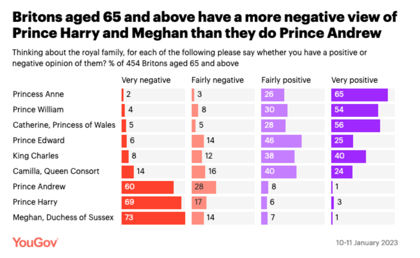
Figure 5: Nine ordinal distributions, one for each major member of the British royal family, all of them using an ordinal codeframe of 4 classes (from VeryNegative to VeryPositive).

A second example is the one illustrated in Figure 6, which concerns a survey of the public opinion on British politician Keir Starmer; here the four ordinal distributions are less smooth than those of the previous example because they exhibit an upward hump in the three middle classes, but they are all fairly smooth elsewhere. Here, $\xi_{1}(\mathbf{p}_{\sigma})$ ranges in [.040,.069] and averages .051.

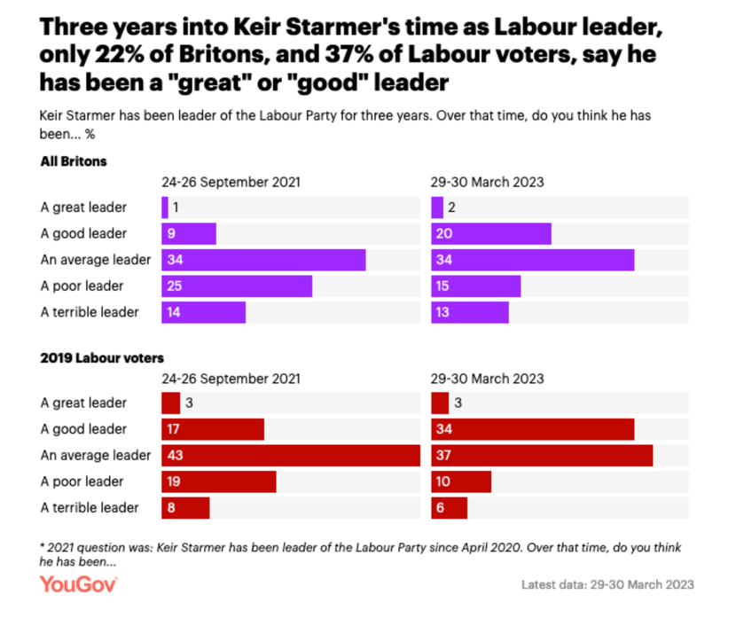
Figure 6: Four ordinal distributions about public opinion on Keir Starmer, all of them using an ordinal codeframe of 5 classes (from GreatLeader to TerribleLeader).

Our third example (see Figure 7) displays a situation similar to the one illustrated by our first one. This is about the public opinion on how good the government of British Prime Minister Rishi Sunak was in delivering his pledges, and displays five ordinal distributions on a 5-point scale, ranging from VeryWell to VeryBadly; here, all the distributions are very smooth, with $\xi_{1}(\mathbf{p}_{\sigma})$ ranging in [.001,.024] and averaging .009.

Figure 7: Five ordinal distributions about public opinion on how good the government of British Prime Minister Rishi Sunak was in delivering his pledges, all of them using an ordinal codeframe of 5 classes (from VeryWell to VeryBadly).

All in all, this is further evidence, although of an anecdotal nature, that the basic intuition on which our methods rest, i.e., that ordinal distributions tend to be fairly smooth, is indeed verified in practice.

Appendix B Other results

The following results complete the experiments we have shown in the main paper.

B.1 RNOD-based evaluation of our experiments

We have repeated all of our experiments by replacing the NMD evaluation function with the RNOD evaluation function discussed in Section 3.2. Note that by adopting RNOD we are not simply replacing the evaluation measure, but also the criterion for model selection. That is to say, we re-run all the experiments anew, this time optimizing hyperparameters by minimizing RNOD in place of NMD.

From examining the RNOD results from Tables 5 and 6, we may note that, while some methods change positions in the ranking, as compared to their ranks in terms of NMD, the general conclusions from the NMD evaluation in the main paper also hold in terms of RNOD.

Table 5: Same as Table 3 (Amazon-OQ-BK data) but using RNOD (see Equation 43) instead of NMD as the evaluation measure.

		APP	APP-OQ	real
	CC	${.1158\pm.0463}$	${.0835\pm.0280}$	${.0511\pm.0303}$
	PCC	${.1324\pm.0515}$	${.0974\pm.0333}$	${.0575\pm.0313}$
	ACC	${.0675\pm.0317}$	${.0505\pm.0241}$	${.0338\pm.0184}$
	PACC	${.0623\pm.0275}$	${.0474\pm.0198}$	${.0334\pm.0177}$
	HDx	${.0592\pm.0248}$	${.0469\pm.0199}$	${.0373\pm.0200}$
	HDy	${.0611\pm.0271}$	${.0473\pm.0205}$	${.0363\pm.0209}$
	SLD	${.0469\pm.0254}$	$\mathbf{.0414\pm.0184}$	$\mathbf{.0318\pm.0162}$
	OQT	${.1448\pm.0622}$	${.1052\pm.0377}$	${.0592\pm.0320}$
	ARC	${.1297\pm.0570}$	${.0947\pm.0349}$	${.0477\pm.0272}$
	IBU	${.0692\pm.0301}$	${.0510\pm.0193}$	${.0338\pm.0182}$
	RUN	${.0669\pm.0298}$	${.0498\pm.0198}$	${.0338\pm.0184}$
	EDy	${.0663\pm.0292}$	${.0506\pm.0213}$	${.0379\pm.0199}$
	PDF	${.0681\pm.0301}$	${.0525\pm.0226}$	${.0378\pm.0204}$
	o-ACC	${.0675\pm.0317}$	${.0505\pm.0241}$	${.0338\pm.0184}$
	o-PACC	${.0624\pm.0275}$	${.0475\pm.0198}$	${.0334\pm.0177}$
	o-HDx	${.0592\pm.0248}$	${.0469\pm.0199}$	${.0372\pm.0199}$
	o-HDy	${.0611\pm.0271}$	${.0473\pm.0205}$	${.0363\pm.0207}$
	o-SLD	$\mathbf{.0418\pm.0208}$	${.0421\pm.0182}$	${.0321\pm.0159}$
	o-EDy	${.0647\pm.0284}$	${.0496\pm.0213}$	${.0393\pm.0201}$
	o-PDF	${.0660\pm.0290}$	${.0513\pm.0228}$	${.0387\pm.0206}$

Table 6: Same as Table 4 (Fact-OQ data) but using RNOD (see Equation 43) instead of NMD as the evaluation measure.

		APP	APP-OQ	real
	CC	${.1175\pm.0323}$	${.0757\pm.0155}$	${.1020\pm.0067}$
	PCC	${.1279\pm.0325}$	${.0848\pm.0188}$	${.1138\pm.0051}$
	ACC	${.1061\pm.0410}$	${.1113\pm.0359}$	${.0899\pm.0590}$
	PACC	${.0887\pm.0357}$	${.0958\pm.0359}$	${.0678\pm.0272}$
	HDx	${.1832\pm.0628}$	${.1660\pm.0553}$	${.2067\pm.0708}$
	HDy	${.0913\pm.0404}$	${.0943\pm.0331}$	${.0719\pm.0494}$
	SLD	${.0751\pm.0265}$	${.0594\pm.0198}$	${.0493\pm.0190}$
	OQT	${.1323\pm.0321}$	${.0909\pm.0200}$	${.0940\pm.0052}$
	ARC	${.1174\pm.0309}$	${.0767\pm.0202}$	${.0861\pm.0065}$
	IBU	${.0805\pm.0272}$	${.0556\pm.0110}$	${.0449\pm.0086}$
	RUN	${.0877\pm.0287}$	${.0588\pm.0116}$	${.0441\pm.0138}$
	EDy	${.0869\pm.0302}$	${.0676\pm.0210}$	${.0431\pm.0098}$
	PDF	${.1070\pm.0361}$	${.1059\pm.0334}$	${.0658\pm.0200}$
	o-ACC	${.0880\pm.0295}$	${.0555\pm.0106}$	${.0425\pm.0083}$
	o-PACC	${.0772\pm.0271}$	$\mathbf{.0470\pm.0114}$	$\mathbf{.0279\pm.0087}$
	o-HDx	${.1195\pm.0417}$	${.0680\pm.0156}$	${.0669\pm.1113}$
	o-HDy	${.0884\pm.0384}$	$\mathbf{.0475\pm.0124}$	${.0300\pm.0123}$
	o-SLD	$\mathbf{.0707\pm.0252}$	${.0507\pm.0112}$	${.0433\pm.0092}$
	o-EDy	${.0827\pm.0279}$	${.0545\pm.0147}$	${.0379\pm.0127}$
	o-PDF	${.0937\pm.0318}$	${.0538\pm.0118}$	${.0308\pm.0098}$

B.2 Results on other datasets

We have repeated our experiments from Tables 3 and 4 with four additional datasets that we have obtained from the UCI machine learning repository and from OpenML. We discuss these additional datasets here, in the appendix, because they have two disadvantages, as compared to our main datasets Amazon-OQ-BK and Fact-OQ.

First, the additional datasets do not have separate “real” samples that we could predict or use to determine an appropriate percentage for APP-OQ. Therefore, we have to omit the real evaluation protocol and we have to make an ad-hoc choice about the percentage of APP samples that we maintain in APP-OQ. We set this percentage to 20%, which lies between the 50% used for Amazon-OQ-BK and the 5% used for Fact-OQ.

The second disadvantage of the additional datasets is that their original purpose is not OQ, not even ordinal classification, but regression. Therefore, we have equidistantly binned the range of their target variables to 10 ordinal classes that we can predict in OQ. We have chosen to use binned regression datasets because we were not able to find datasets that are originally ordinal and have a sufficient number of data items; in fact, APP and APP-OQ require huge datasets for drawing a training set and two large pools, one for validation and one for testing.

The results of our experiments with the additional data are reported in Tables 7 and 8. Despite the shortcomings of the employed data, these results confirm our main conclusions on OQ: the regularized methods consistently improve over their original non-regularized versions, at least being on par with these versions.

Table 7: Results, evaluated in terms of NMD, of the experiments performed on additional datasets obtained from OpenML.

method	OpenMl-Yolanda-OQ			OpenMl-fried-OQ
	APP	APP-OQ (20%)		APP	APP-OQ (20%)
CC	${.0847\pm.0240}$	${.0836\pm.0230}$		${.0282\pm.0067}$	${.0230\pm.0055}$
PCC	${.1111\pm.0461}$	${.1081\pm.0484}$		${.0459\pm.0105}$	${.0408\pm.0108}$
ACC	${.0751\pm.0214}$	${.0740\pm.0186}$		${.0166\pm.0059}$	${.0180\pm.0058}$
PACC	${.0593\pm.0210}$	${.0536\pm.0169}$		${.0150\pm.0063}$	${.0164\pm.0054}$
HDx	${.0596\pm.0223}$	${.0578\pm.0308}$		${.0963\pm.0803}$	${.0993\pm.0860}$
HDy	${.0615\pm.0267}$	${.0593\pm.0359}$		${.0132\pm.0093}$	${.0139\pm.0042}$
SLD	${.0789\pm.0170}$	${.0792\pm.0152}$		${.0278\pm.0050}$	${.0291\pm.0049}$
OQT	${.2639\pm.0705}$	${.2602\pm.0710}$		${.0413\pm.0100}$	${.0345\pm.0079}$
ARC	${.2180\pm.0554}$	${.2158\pm.0557}$		${.0441\pm.0174}$	${.0427\pm.0191}$
IBU	${.0544\pm.0163}$	${.0480\pm.0163}$		${.0130\pm.0040}$	${.0129\pm.0033}$
RUN	${.0538\pm.0147}$	${.0466\pm.0151}$		${.0163\pm.0058}$	${.0207\pm.0058}$
EDy	${.0532\pm.0151}$	${.0515\pm.0147}$		${.0133\pm.0042}$	${.0119\pm.0033}$
PDF	${.0964\pm.0293}$	${.0954\pm.0265}$		${.0132\pm.0037}$	${.0126\pm.0034}$
o-ACC	${.0526\pm.0152}$	${.0443\pm.0138}$		${.0165\pm.0059}$	${.0130\pm.0039}$
o-PACC	$\mathbf{.0429\pm.0123}$	$\mathbf{.0328\pm.0096}$		${.0149\pm.0063}$	${.0123\pm.0029}$
o-HDx	${.0529\pm.0156}$	${.0457\pm.0161}$		${.0688\pm.0884}$	${.0704\pm.1042}$
o-HDy	${.0471\pm.0387}$	${.0371\pm.0294}$		${.0130\pm.0120}$	${.0116\pm.0028}$
o-SLD	${.0658\pm.0181}$	${.0657\pm.0181}$		${.0249\pm.0049}$	${.0235\pm.0047}$
o-EDy	${.0480\pm.0142}$	${.0434\pm.0136}$		${.0093\pm.0030}$	$\mathbf{.0078\pm.0023}$
o-PDF	${.0524\pm.0159}$	${.0454\pm.0161}$		$\mathbf{.0087\pm.0049}$	${.0083\pm.0027}$

Table 8: Results, evaluated in terms of NMD, of the experiments performed on additional datasets obtained from UCI.

method	Uci-blog-feedback-OQ			Uci-online-news-popularity-OQ
	APP	APP-OQ (20%)		APP	APP-OQ (20%)
CC	${.0850\pm.0325}$	${.0780\pm.0310}$		${.1357\pm.0420}$	${.1226\pm.0386}$
PCC	${.0894\pm.0370}$	${.0835\pm.0365}$		${.1018\pm.0446}$	${.0970\pm.0456}$
ACC	${.0773\pm.0299}$	${.1402\pm.0410}$		${.1042\pm.0464}$	${.0996\pm.0478}$
PACC	${.1099\pm.0455}$	${.1089\pm.0419}$		${.0850\pm.0325}$	${.0865\pm.0362}$
HDx	${.1045\pm.0509}$	${.0973\pm.0518}$		${.2075\pm.1133}$	${.1966\pm.1251}$
HDy	${.0704\pm.0455}$	${.0891\pm.0530}$		${.1175\pm.0523}$	${.1120\pm.0579}$
SLD	$\mathbf{.0454\pm.0150}$	$\mathbf{.0389\pm.0116}$		${.0892\pm.0337}$	${.0810\pm.0299}$
OQT	${.0953\pm.0379}$	${.0842\pm.0350}$		${.2007\pm.0594}$	${.1915\pm.0591}$
ARC	${.1248\pm.0368}$	${.1073\pm.0324}$		${.3192\pm.0843}$	${.3209\pm.0837}$
IBU	${.0631\pm.0217}$	${.0557\pm.0189}$		${.0814\pm.0285}$	$\mathbf{.0714\pm.0279}$
RUN	${.0821\pm.0249}$	${.0765\pm.0232}$		${.0881\pm.0349}$	${.0865\pm.0368}$
EDy	${.0563\pm.0189}$	${.0497\pm.0150}$		${.1356\pm.0397}$	${.1388\pm.0384}$
PDF	${.0652\pm.0209}$	${.0584\pm.0181}$		${.1220\pm.0419}$	${.1147\pm.0382}$
o-ACC	${.0681\pm.0198}$	${.0623\pm.0200}$		${.0940\pm.0385}$	${.0941\pm.0413}$
o-PACC	${.0744\pm.0287}$	${.0658\pm.0249}$		${.0808\pm.0296}$	$\mathbf{.0723\pm.0334}$
o-HDx	${.0982\pm.0506}$	${.0888\pm.0534}$		${.1075\pm.1158}$	$\mathbf{.1009\pm.1305}$
o-HDy	${.0645\pm.0338}$	${.0617\pm.0342}$		${.0905\pm.0353}$	${.0795\pm.0304}$
o-SLD	$\mathbf{.0454\pm.0151}$	$\mathbf{.0387\pm.0116}$		$\mathbf{.0769\pm.0292}$	$\mathbf{.0698\pm.0275}$
o-EDy	${.0944\pm.0348}$	${.0833\pm.0224}$		$\mathbf{.0764\pm.0264}$	$\mathbf{.0675\pm.0256}$
o-PDF	${.0967\pm.0331}$	${.0931\pm.0298}$		${.0821\pm.0295}$	${.0711\pm.0260}$

B.3 Hyperparameter grids

In our experiments, each method has the opportunity to optimize its hyperparameters on the validation samples of the respective evaluation protocol. These hyperparameters consist of the parameters of the quantifier and of the parameters of the classifier, with which the quantifier is equipped. After taking out preliminary experiments, which we omit here for conciseness, we have chosen slightly different hyperparameter grids for the different datasets.

To this end, Tables 9 and 10 present the parameters for the Amazon-OQ-BK dataset. For instance, CC can choose between 10 hyperparameter configurations of the classifier (2 class weights $\times$ 5 regularization strengths) but does not introduce additional parameters on the quantification level. We note that preliminary results revealed that the fraction of held-out data does not considerably affect the results of OQT and ARC. Therefore, and since those methods are computationally expensive, we decided to fix the proportion of the held-out split to $\frac{1}{3}$ and do not include this hyperparameter in the exploration.

Tables 9 and 11 present the parameters for the Fact-OQ data. For conciseness, they also contain the parameters for the UCI and OpenML datasets.

Table 9: Hyperparameter grid used for the optimization of the quantification methods employed in the experiments reported in Tables 3 and 4.

method	parameter	values
CC	no parameters
PCC	no parameters
ACC	no parameters
PACC	no parameters
HDx	number of bins per feature	$\{2,3,4\}$
HDy	number of bins per class	$\{2,4\}$
SLD	no parameters
OQT	fraction of held-out data	$\{\frac{1}{3}\}$
ARC	fraction of held-out data	$\{\frac{1}{3}\}$
RUN	$\tau$	$\{$1e-3, 1e-1, 1e1$\}$
IBU	order of polynomial	$\{0,1\}$
	interpolation factor	$\{1e-2,1e-1\}$
EDy	ground distance	{MD}
PDF	number of bins per class	$\{5,10\}$
o-ACC	$\tau$	$\{$1e-5, 1e-3, 1e-1$\}$
o-PACC	$\tau$	$\{$1e-5, 1e-3, 1e-1$\}$
o-HDx	number of bins per feature	$\{2,3,4\}$
	$\tau$	$\{$1e-5, 1e-3, 1e-1$\}$
o-HDy	number of bins per class	$\{2,4\}$
	$\tau$	$\{$1e-5, 1e-3, 1e-1$\}$
o-SLD	order of polynomial	$\{0,1\}$
	interpolation factor	$\{$1e-2, 1e-1$\}$
o-EDy	ground distance	{MD}
	$\tau$	$\{$1e-5, 1e-3, 1e-1$\}$
o-PDF	number of bins per class	$\{5,10\}$
	$\tau$	$\{$1e-5, 1e-3, 1e-1$\}$

Table 10: Hyperparameter grid used for the optimization of the classifiers employed in the Amazon-OQ-BK experiments reported in Table 3.

classifier	parameter	values
Logistic Regression	class weight	{balanced, unbalanced}
	regularization parameter $C$	$\{0.001,0.01,0.1,1.0,10.0\}$

Table 11: Hyperparameter grids used for the optimization of the classifiers employed in the Fact-OQ, OpenML, and UCI experiments reported in Tables 4, 7 and 8.

classifier	parameter	values
Random Forests	class weight	{balanced, unbalanced}
	splitting criterion	{Gini index, Entropy}
	maximum depth	$\{4,8,12\}$

References

- Aad et al. (2021) Aad G, Abbott B, Abbott DC, et al. (2021) Measurements of the inclusive and differential production cross sections of a top-quark–antiquark pair in association with a Z boson at TeV with the ATLAS detector. European Physics Journal C 81(8)
- Aartsen et al. (2017) Aartsen MG, Ackermann M, Adams J, et al. (2017) Measurement of the energy spectrum with IceCube-79. European Physics Journal C 77(692), DOI 10.1140/epjc/s10052-017-5261-3
- Aleksić et al. (2015) Aleksić J, et al. (2015) Measurement of the Crab Nebula spectrum over three decades in energy with the MAGIC telescopes. Journal of High Energy Astrophysics 5-6:30–38, DOI https://doi.org/10.1016/j.jheap.2015.01.002
- Anderhub et al. (2013) Anderhub H, Backes M, Biland A, et al. (2013) Design and operation of FACT, the first G-APD Cherenkov telescope. Journal of Instrumentation 8(6), DOI 10.1088/1748-0221/8/06/P06008
- Bella et al. (2010) Bella A, Ferri C, Hernández-Orallo J, Ramírez-Quintana MJ (2010) Quantification via probability estimators. In: Proceedings of the 11th IEEE International Conference on Data Mining (ICDM 2010), Sydney, AU, pp 737–742, DOI 10.1109/icdm.2010.75
- Blobel (1985) Blobel V (1985) Unfolding methods in high-energy physics experiments. Tech. Rep. DESY-84-118, CERN, Geneva, CH, DOI 10.5170/CERN-1985-009.88
- Blobel (2002) Blobel V (2002) An unfolding method for high-energy physics experiments. In: Proceedings of the Conference on Advanced Statistical Techniques in Particle Physics, Durham, UK, pp 258–267, extended version available at https://www.desy.de/~sschmitt/blobel/punfold.ps
- Börner et al. (2017) Börner M, Hoinka T, Meier M, Menne T, Rhode W, Morik K (2017) Measurement/simulation mismatches and multivariate data discretization in the machine learning era. In: Proceedings of the 27th Conference on Astronomical Data Analysis Software and Systems (ADASS 2017), Santiago, CL, pp 431–434
- Breiman (1996) Breiman L (1996) Out-of-bag estimation. Tech. rep., Department of Statistics, University of California, Berkeley, US
- Bunse (2022a) Bunse M (2022a) On multi-class extensions of adjusted classify and count. In: Proceedings of the 2nd International Workshop on Learning to Quantify (LQ 2022), Grenoble, IT, pp 43–50
- Bunse (2022b) Bunse M (2022b) Unification of algorithms for quantification and unfolding. In: Proceedings of the Workshop on Machine Learning for Astroparticle Physics and Astronomy, pp 459–468, DOI 10.18420/INF2022˙37
- Bunse et al. (2018) Bunse M, Piatkowski N, Morik K, Ruhe T, Rhode W (2018) Unification of deconvolution algorithms for Cherenkov astronomy. In: Proceedings of the 5th IEEE International Conference on Data Science and Advanced Analytics (DSAA 2018), Torino, IT, pp 21–30, DOI 10.1109/DSAA.2018.00012
- Bunse et al. (2022) Bunse M, Moreo A, Sebastiani F, Senz M (2022) Ordinal quantification through regularization. In: Proceedings of the 33rd European Conference on Machine Learning and Principles and Practice of Knowledge Discovery in Databases (ECML / PKDD 2022), Grenoble, FR, pp 36–52
- Castaño et al. (2023) Castaño A, González P, González JA, del Coz JJ (2023) Matching distributions algorithms based on the Earth mover’s distance for ordinal quantification. IEEE Transactions on Neural Networks and Learning Systems DOI 10.1109/TNNLS.2022.3179355, forthcoming
- Da San Martino et al. (2016) Da San Martino G, Gao W, Sebastiani F (2016) Ordinal text quantification. In: Proceedings of the 39th ACM Conference on Research and Development in Information Retrieval (SIGIR 2016), Pisa, IT, pp 937–940, DOI 10.1145/2911451.2914749
- D’Agostini (1995) D’Agostini G (1995) A multidimensional unfolding method based on Bayes’ theorem. Nuclear Instruments and Methods in Physics Research: Section A 362(2-3):487–498
- D’Agostini (2010) D’Agostini G (2010) Improved iterative Bayesian unfolding. ArXiv:1010.0632 [physics.data-an]
- Esuli (2016) Esuli A (2016) ISTI-CNR at SemEval-2016 Task 4: Quantification on an ordinal scale. In: Proceedings of the 10th International Workshop on Semantic Evaluation (SemEval 2016), San Diego, US, pp 92–95, DOI 10.18653/v1/s16-1011
- Esuli and Sebastiani (2010) Esuli A, Sebastiani F (2010) Sentiment quantification. IEEE Intelligent Systems 25(4):72–75
- Esuli et al. (2018) Esuli A, Moreo A, Sebastiani F (2018) A recurrent neural network for sentiment quantification. In: Proceedings of the 27th ACM International Conference on Information and Knowledge Management (CIKM 2018), Torino, IT, pp 1775–1778, DOI 10.1145/3269206.3269287
- Esuli et al. (2022) Esuli A, Moreo A, Sebastiani F (2022) LeQua@CLEF2022: Learning to Quantify. In: Proceedings of the 44th European Conference on Information Retrieval (ECIR 2022), Stavanger, NO, pp 374–381, DOI 10.1007/978-3-030-72240-1“˙6
- Esuli et al. (2023) Esuli A, Fabris A, Moreo A, Sebastiani F (2023) Learning to quantify. Springer Nature, Cham, CH
- Forman (2005) Forman G (2005) Counting positives accurately despite inaccurate classification. In: Proceedings of the 16th European Conference on Machine Learning (ECML 2005), Porto, PT, pp 564–575, DOI 10.1007/11564096“˙55
- Gao and Sebastiani (2016) Gao W, Sebastiani F (2016) From classification to quantification in tweet sentiment analysis. Social Network Analysis and Mining 6(19):1–22, DOI 10.1007/s13278-016-0327-z
- González et al. (2017) González P, Castaño A, Chawla NV, del Coz JJ (2017) A review on quantification learning. ACM Computing Surveys 50(5):74:1–74:40, DOI 10.1145/3117807
- González and del Coz (2021) González P, del Coz JJ (2021) Histogram-based deep neural network for quantification (abstract). In: Proceedings of the 1st International Workshop on Learning to Quantify (LQ 2021), Virtual Event
- González-Castro et al. (2013) González-Castro V, Alaiz-Rodríguez R, Alegre E (2013) Class distribution estimation based on the Hellinger distance. Information Sciences 218:146–164, DOI 10.1016/j.ins.2012.05.028
- Higashinaka et al. (2017) Higashinaka R, Funakoshi K, Inaba M, Tsunomori Y, Takahashi T, Kaji N (2017) Overview of the 3rd Dialogue Breakdown Detection challenge. In: Proceedings of the 6th Dialog System Technology Challenge, Long Beach, US
- Hoecker and Kartvelishvili (1996) Hoecker A, Kartvelishvili V (1996) SVD approach to data unfolding. Nuclear Instruments and Methods in Physics Research: Section A 372(3):469–481
- Kawakubo et al. (2016) Kawakubo H, du Plessis MC, Sugiyama M (2016) Computationally efficient class-prior estimation under class balance change using energy distance. IEICE Transactions on Information Systems 99-D(1):176–186, DOI 10.1587/transinf.2015EDP7212
- Liu et al. (2019) Liu Y, Ott M, Goyal N, Du J, Joshi M, Chen D, Levy O, Lewis M, Zettlemoyer L, Stoyanov V (2019) RoBERTa: A robustly optimized BERT pretraining approach. ArXiv:1907.11692
- McAuley et al. (2015) McAuley JJ, Targett C, Shi Q, van den Hengel A (2015) Image-based recommendations on styles and substitutes. In: Proceedings of the 38th International ACM Conference on Research and Development in Information Retrieval (SIGIR 2015), Santiago, CL, pp 43–52, DOI 10.1145/2766462.2767755
- Moreno-Torres et al. (2012) Moreno-Torres JG, Raeder T, Alaíz-Rodríguez R, Chawla NV, Herrera F (2012) A unifying view on dataset shift in classification. Pattern Recognition 45(1):521–530, DOI 10.1016/j.patcog.2011.06.019
- Mueller and Siltanen (2012) Mueller JL, Siltanen S (2012) Linear and nonlinear inverse problems with practical applications. Society for Industrial and Applied Mathematics, Philadelphia, US, DOI 10.1137/1.9781611972344
- Nachman et al. (2020) Nachman B, Urbanek M, de Jong WA, Bauer CW (2020) Unfolding quantum computer readout noise. npj Quantum Information 6(84), DOI 0.1038/s41534-020-00309-7
- Nakov et al. (2016) Nakov P, Ritter A, Rosenthal S, Sebastiani F, Stoyanov V (2016) SemEval-2016 Task 4: Sentiment analysis in Twitter. In: Proceedings of the 10th International Workshop on Semantic Evaluation (SemEval 2016), San Diego, US, pp 1–18, DOI 10.18653/v1/s16-1001
- Nöthe et al. (2017) Nöthe M, Adam J, Ahnen ML, et al. (2017) FACT – Performance of the first Cherenkov telescope observing with SiPMs. In: Proceedings of the 35th International Cosmic Ray Conference (ICRC 2017), pp Busan, KR
- Pedregosa et al. (2017) Pedregosa F, Bach F, Gramfort A (2017) On the consistency of ordinal regression methods. Journal of Machine Learning Research 18:55:1–55:35
- Pérez-Gállego et al. (2019) Pérez-Gállego P, Castaño A, Quevedo JR, del Coz JJ (2019) Dynamic ensemble selection for quantification tasks. Information Fusion 45:1–15, DOI 10.1016/j.inffus.2018.01.001
- Rennie and Srebro (2005) Rennie JD, Srebro N (2005) Loss functions for preference levels: Regression with discrete ordered labels. In: Proceedings of the IJCAI 2005 Workshop on Advances in Preference Handling
- Rosenthal et al. (2017) Rosenthal S, Farra N, Nakov P (2017) SemEval-2017 Task 4: Sentiment analysis in Twitter. In: Proceedings of the 11th International Workshop on Semantic Evaluation (SemEval 2017), Vancouver, CA, pp 502–518, DOI 10.18653/v1/s17-2088
- Rubner et al. (1998) Rubner Y, Tomasi C, Guibas LJ (1998) A metric for distributions with applications to image databases. In: Proceedings of the 6th International Conference on Computer Vision (ICCV 1998), Mumbai, IN, pp 59–66
- Ruhe et al. (2013) Ruhe T, Schmitz M, Voigt T, Wornowizki M (2013) DSEA: A data mining approach to unfolding. In: Proceedings of the 33rd International Cosmic Ray Conference (ICRC 2013), Rio de Janeiro, BR, pp 3354–3357
- Saerens et al. (2002) Saerens M, Latinne P, Decaestecker C (2002) Adjusting the outputs of a classifier to new a priori probabilities: A simple procedure. Neural Computation 14(1):21–41, DOI 10.1162/089976602753284446
- Sakai (2018) Sakai T (2018) Comparing two binned probability distributions for information access evaluation. In: Proceedings of the 41st International ACM Conference on Research and Development in Information Retrieval (SIGIR 2018), Ann Arbor, US, pp 1073–1076, DOI 10.1145/3209978.3210073
- Sakai (2021) Sakai T (2021) A closer look at evaluation measures for ordinal quantification. In: Proceedings of the CIKM 2021 Workshop on Learning to Quantify, Virtual Event
- Schmelling (1994) Schmelling M (1994) The method of reduced cross-entropy: A general approach to unfold probability distributions. Nuclear Instruments and Methods in Physics Research Section A: Accelerators, Spectrometers, Detectors and Associated Equipment 340(2):400–412
- Schmitt (2012) Schmitt S (2012) TUnfold, an algorithm for correcting migration effects in high-energy physics. Journal of Instrumentation 7(10)
- Smith and Tromble (2004) Smith NA, Tromble RW (2004) Sampling uniformly from the unit simplex. Tech. rep., Johns Hopkins University, https://www.cs.cmu.edu/~nasmith/papers/smith+tromble.tr04.pdf
- Werman et al. (1985) Werman M, Peleg S, Rosenfeld A (1985) A distance metric for multidimensional histograms. Computer Vision, Graphics, and Image Processing 32:328–336
- Zeng et al. (2019) Zeng Z, Kato S, Sakai T (2019) Overview of the NTCIR-14 Short Text Conversation task: Dialogue Quality and Nugget Detection subtasks. In: Proceedings of the 14th Workshop on NII Testbeds and Community for Information access Research (NTCIR 2019), Tokyo, JP, pp 289–315
- Zeng et al. (2020) Zeng Z, Kato S, Sakai T, Kang I (2020) Overview of the NTCIR-15 Dialogue Evaluation task (DialEval-1). In: Proceedings of the 15th Workshop on NII Testbeds and Community for Information access Research (NTCIR 2020), Tokyo, JP, pp 13–34