Graph Condensation via Eigenbasis Matching

Abstract.

The increasing amount of graph data places requirements on the efficiency and scalability of graph neural networks (GNNs), despite their effectiveness in various graph-related applications. Recently, the emerging graph condensation (GC) sheds light on reducing the computational cost of GNNs from a data perspective. It aims to replace the real large graph with a significantly smaller synthetic graph so that GNNs trained on both graphs exhibit comparable performance. However, our empirical investigation reveals that existing GC methods suffer from poor generalization, i.e., different GNNs trained on the same synthetic graph have obvious performance gaps. What factors hinder the generalization of GC and how can we mitigate it? To answer this question, we commence with a detailed analysis and observe that GNNs will inject spectrum bias into the synthetic graph, resulting in a distribution shift. To tackle this issue, we propose eigenbasis matching for spectrum-free graph condensation, named GCEM, which has two key steps: First, GCEM matches the eigenbasis of the real and synthetic graphs, rather than the graph structure, which eliminates the spectrum bias of GNNs. Subsequently, GCEM leverages the spectrum of the real graph and the synthetic eigenbasis to construct the synthetic graph, thereby preserving the essential structural information. We theoretically demonstrate that the synthetic graph generated by GCEM maintains the spectral similarity, i.e., total variation, of the real graph. Extensive experiments conducted on five graph datasets verify that GCEM not only achieves state-of-the-art performance over baselines but also significantly narrows the performance gaps between different GNNs.

1. Introduction

Graph, as a ubiquitous data structure, has been widely used to represent and explore the complex relationships between objectives. Among various graph learning methods, graph neural networks (GNNs) have become the de facto framework to encode both graph structures and node features, and play a vital role in the diverse web applications (app1; app2; app3). However, the swift evolution of the World Wide Web has led to the generation of vast quantities of data, which challenges the efficiency and scalability of GNNs.

Recently, graph condensation (GC) has shown great potential in reducing the computational cost (GCond; GCDM; SFGC; MCond; DosCond; KIDD). The goal of GC is to generate a small yet informative synthetic graph by matching the model gradients (GCond; DosCond; SFGC) or data distributions (GCDM) between the real and synthetic graphs. Once generated, GNNs trained on both graphs will have comparable performance, thus accelerating the training of GNNs. Under the same compression ratio, existing GC methods have an average of 5-30% performance improvement over the traditional graph reduction algorithms, such as core-set (core_set1; core_set2) and graph coarsening (coarsening1; coarsening2). Despite the remarkable performance, the generalization of GC has not been systematically explored. Can different GNNs trained on the same synthetic graph consistently perform well in the evaluation phase? This is an important question because the synthetic graph should benefit a variety of GNNs rather than a specific one.

Experimental investigation. To verify the generalization ability, we evaluate the performance of GCOND (GCond), a traditional GC method, on six popular GNNs, belonging to two categories: Spatial GNNs, including GCN (GCN), SGC (SGC), and PPNP (PPNP). Spectral GNNs, including ChebyNet (ChebNet), BernNet (BernNet), and GPR-GNN (GPR-GNN). Specifically, these six GNNs take turns serving as the condensation model for synthetic graph generation. Then we train all GNNs in the synthetic graphs and evaluate their performance. The results are presented in Table 1, and it is evident that the optimal performance is achieved when the condensation and evaluation stages share the same GNN, as demonstrated by the diagonal results. Furthermore, in Table 2, we report the category-level results by averaging the performance of spatial and spectral GNNs, respectively. It can be observed that the performance gap increases when the condensation and evaluation models have different architectures. More details can be seen in Appendix A. This investigation shows that existing GC methods have an inherent generalization defect and fail to consistently benefit different GNNs. Once the weakness is identified, a natural question is what exactly affects the generalization of GC and how can we prevent it?

Table 1. Node classification accuracy (%) of GCOND (GCond) with different condensation (C) and evaluation (E) models on Cora dataset. Bold indicates the best performance in each row.

C ${\diagdown}$ E	SGC	GCN	PPNP	Cheb.	Bern.	GPR.
SGC	72.64	70.20	71.54	62.50	61.74	69.06
GCN	69.64	76.02	75.54	71.30	72.10	75.82
PPNP	73.22	75.26	76.88	61.14	63.24	74.34
Cheb.	66.16	66.40	70.44	71.82	71.68	75.72
Bern.	51.40	53.38	69.12	70.06	71.62	70.66
GPR.	70.74	71.02	72.94	73.28	72.80	75.34

• Note: We do not use graph sampling in this experiment. Therefore, the performance will be slightly lower than the results in the original paper.

Table 2. The average performance of spatial and spectral GNNs. Mean accuracy (%) ± standard deviation.

C ${\diagdown}$ E	Spatial	Spectral
Spatial	73.44±2.48	67.92±5.47
Spectral	65.73±7.43	72.55±1.84

Generally, a graph can be represented by its spectrum, i.e., eigenvalues, and the corresponding eigenbasis, i.e., a set of eigenvectors. Both spatial and spectral GNNs learn node representations by changing the spectrum of graphs (Unified; spectral_survey). Although this paradigm has been proven effective for node classification, it may be harmful to GC due to the spectrum preferences of GNNs. Essentially, altering the spectrum will affect the importance of different eigenvectors in the eigenbasis, consequently leading to modifications in node features. Intuitively, if GNN operates as a low-pass filter (SGC; low-pass), it will emphasize the low-frequency information in node features rather than the entire spectrum. In Section 3, we present a more detailed analysis and observe that the condensation GNNs will inject spectrum bias into the synthetic graph during the condensation process, resulting in a distribution shift between the real and synthetic graphs.

Challenges and present work. To mitigate the generalization defect, in this paper, we investigate spectrum-free graph condensation. In particular, we aim to generate the eigenbasis of the synthetic graph to get rid of the spectrum bias of GNNs. This problem is non-trivial due to the following two challenges.

Firstly, how to match the eigenbasis of the real and synthetic graphs? The eigenbasis consists of a set of Laplacian eigenvectors, representing the underlying structures of the corresponding graph. Aligning the eigenbasis of the real and synthetic graphs can help them maintain similar representation spaces. Nevertheless, the number and shape of the eigenvectors in the eigenbasis are equal to the number of nodes in a graph. Therefore, it is infeasible to directly match the eigenbasis of the real and synthetic graphs, due to their difference in graph size.

Secondly, how to make the synthetic graph preserve the important structural information of the real graph? Structural information, such as global shape and local connectivity, plays a vital role in graph generation (Spectre). Previous condensation methods employ neural networks, e.g., multilayer perceptron (MLP), to predict the graph structures, or learn a structure-free synthetic graph. However, without any prior knowledge, it is intractable for neural networks to directly encode the structural information of graphs.

To tackle the aforementioned challenges, we propose a novel Graph Condensation framework through Eigenbasis Matching, named GCEM. To address the first challenge posed by the different graph sizes, GCEM aims to match the synthetic eigenvectors with a few important eigenvectors of the real graph, such as eigenvectors with smaller or larger eigenvalues, which eliminates the difference in the number of eigenvectors. Moreover, GCEM aligns the node features in the subspaces defined by the eigenvectors of the real and synthetic graphs, which solves the difference in the shape of eigenvectors, as the node features in both graphs have the same dimensions. Once the eigenbasis is generated, GCEM constructs the synthetic graph by leveraging the spectrum of the real graph, which naturally preserves some global structural properties. For example, the second smallest eigenvalue in the spectrum represents the connectivity of a graph (spectral_graph_theory). Furthermore, with some additional regularization terms, the synthetic graphs generated by GCEM show great effectiveness and generalization.

Contributions. Our contributions are summarized as follows:

1. To the best of our knowledge, we are the first to systematically analyze the generalization issue of GC and observe that existing methods inject spectrum bias into the synthetic graph during the condensation process, resulting in a distribution shift.

2. We propose a novel graph condensation method GCEM, which generates the synthetic graph by learning its eigenbasis, thus avoiding the spectrum bias caused by the condensation GNNs.

3. Theoretically, the synthetic graph generated by GCEM is an $\epsilon$-spectral approximation of the real graph, which preserves its spectral similarity.

4. Extensive experiments on five graph datasets validate the superiority of GCEM over baselines in terms of effectiveness and generalization.

2. Preliminary

Before describing our framework in detail, we first introduce some notations and concepts used in this paper. Specifically, we focus on the node classification task, where the goal is to predict the labels of the nodes in a graph. Assume that there is a graph $\mathcal{G}=(\mathcal{V},\mathcal{E},\mathbf{X})$, where $\mathcal{V}$ is the set of nodes with $|\mathcal{V}|=n$, $\mathcal{E}$ indicates the set of edges, and $\mathbf{X}\in\mathbb{R}^{n\times d}$ is the node feature matrix. The adjacency matrix of $\mathcal{G}$ is defined as $\mathbf{A}\in\{0,1\}^{n\times n}$, where $A_{ij}=1$ if there is an edge between nodes $i$ and $j$, and $A_{ij}=0$ otherwise. The corresponding normalized Laplacian matrix is defined as $\mathbf{L}=\mathbf{I}_{n}-\mathbf{D}^{-\frac{1}{2}}\mathbf{A}\mathbf{D}^{-\frac{1}{2}}$, where $\mathbf{I}_{n}$ is an identity matrix and $\mathbf{D}$ is the degree matrix with $D_{ii}=\sum_{j}A_{ij}$ for $i\in\mathcal{V}$ and $D_{ij}=0$ for $i\neq j$. Without loss of generality, we assume that $\mathcal{G}$ is undirected and all the nodes are connected.

2.1. Eigenbasis and Graph Convolution

Since the normalized graph Laplacian is a real symmetric matrix, it has an orthogonal eigenbasis, $\mathbf{U}=[\mathbf{u}_{1},\cdots,\mathbf{u}_{n}]\in\mathbb{R}^{n\times n}$, consisting of a set of Laplacian eigenvectors. Each eigenvector $\mathbf{u}_{i}\in\mathbb{R}^{n\times 1}$ has a corresponding eigenvalue $\lambda_{i}$, such that $\mathbf{L}\mathbf{u}_{i}=\lambda_{i}\mathbf{u}_{i}$. The normalized graph Laplacian can be represented as $\mathbf{L}=\mathbf{U}\bm{\Lambda}\mathbf{U}^{\top}$, where $\bm{\Lambda}=\text{diag}(\{\lambda_{i}\}_{i=1}^{n})$ and we have $0\leq\lambda_{1}\leq\cdots\leq\lambda_{n}\leq 2$.

The eigenbasis is usually used as the basis of graph Fourier transform and its inverse (GSP), which offers a way to define the graph convolution operator:

(1) $$\mathbf{x}*_{G}f=\mathbf{U}\left(\left(\mathbf{U}^{\top}f\right)\odot\left(\mathbf{U}^{\top}\mathbf{x}\right)\right),$$

where $\mathbf{x}\in\mathbb{R}^{n\times 1}$ is a graph signal and $f$ is a spatial filter. According to the convolution theorem, convolution in the spatial domain $*_{G}$ is equal to the multiplication $\odot$ in the spectral domain.

Replacing the spatial filter $\mathbf{U}^{\top}f$ with a learnable diagonal matrix $\mathbf{G}=\text{diag}(\{g_{i}\}_{i=1}^{n})$ yields the architecture of modern GNNs:

(2) $$\mathbf{x}^{\prime}=\mathbf{U}\mathbf{G}\mathbf{U}^{\top}\mathbf{x}=\sum_{i=1}^{n}g_{i}\mathbf{u}_{i}\mathbf{u}_{i}^{\top}\mathbf{x},$$

where $\mathbf{x}^{\prime}$ is the filtered graph signal. Note that the graph filter $\mathbf{U}\mathbf{G}\mathbf{U}^{\top}$ forms a new graph structure that is a weighted sum of the subspaces of eigenbasis, e.g., $\mathbf{U}\mathbf{G}\mathbf{U}^{\top}=\sum_{i=1}^{n}g_{i}\mathbf{u}_{i}\mathbf{u}_{i}^{\top}$.

2.2. Graph Condensation

Graph condensation aims to generate a graph $\mathcal{G}^{\prime}=(\mathcal{V}^{\prime},\mathcal{E}^{\prime},\mathbf{X}^{\prime})$, where $|\mathcal{V}^{\prime}|=n^{\prime}\ll|\mathcal{V}|=n$ and $\mathbf{X}^{\prime}\in\mathbb{R}^{n^{\prime}\times d}$, enabling GNNs trained on $\mathcal{G}$ and $\mathcal{G}^{\prime}$ to have comparable performance. The compression ratio is defined as $r=n^{\prime}/n$. Existing GC methods can be divided into two categories:

Gradient Matching (GCond; DosCond) generates the synthetic graph and node features by minimizing the differences between model gradients on $\mathcal{G}$ and $\mathcal{G}^{\prime}$, which can be formulated as:

(3) $$\min_{\mathbf{A}^{\prime},\mathbf{X}^{\prime}}\underset{\theta\sim P_{\theta}}{\mathbb{E}}\left[D\left(\nabla_{\theta}\mathcal{L}\left(\Phi_{\theta}\left(\mathbf{A}^{\prime},\mathbf{X}^{\prime}\right),\mathbf{Y}^{\prime}\right),\nabla_{\theta}\mathcal{L}\left(\Phi_{\theta}\left(\mathbf{A},\mathbf{X}\right),\mathbf{Y}\right)\right)\right],$$

where $\Phi_{\theta}$ is the condensation GNNs with parameters $\theta$, $\nabla_{\theta}$ indicates the model gradients, $D$ is a metric to measure their differences, $\mathcal{L}$ is the loss function, and $\mathbf{Y}^{\prime}$ and $\mathbf{Y}$ represent the labels. For clarity, we omit the subscript that indicates the training data.

Distribution Matching (GCDM) aims to align the distributions of node representations in each GNN layer to generate the synthetic graph, which can be expressed as:

(4) $$\min_{\mathbf{A}^{\prime},\mathbf{X}^{\prime}}\sum_{l=1}^{L}D\left(\Phi^{l}_{\theta}\left(\mathbf{A}^{\prime},\mathbf{X}^{\prime}\right),\Phi^{l}_{\theta}\left(\mathbf{A},\mathbf{X}\right)\right),$$

where $\Phi^{l}_{\theta}$ is the $l$-th layer in GNNs.

3. Observation and Motivation

In this section, we give a detailed analysis of the gradient matching methods on graphs, which motivates the design of our method. We start with a vanilla example, which adopts a one-layer GCN as the condensation model and simplifies the objective function into a regression loss:

(5) $$\mathcal{L}=\frac{1}{2}\left\|\mathbf{A}\mathbf{X}\mathbf{W}-\mathbf{Y}\right\|^{2},$$

where $\mathbf{W}$ is the model parameters. The gradients on the real and synthetic graphs are calculated as:

(6) $$\nabla_{\mathbf{W}}={\left(\mathbf{A}\mathbf{X}\right)}^{T}\left(\mathbf{A}\mathbf{X}\mathbf{W}-\mathbf{Y}\right),\ \nabla_{\mathbf{W}}^{\prime}={\left(\mathbf{A}^{\prime}\mathbf{X}^{\prime}\right)}^{T}\left(\mathbf{A^{\prime}}\mathbf{X}^{\prime}\mathbf{W}-\mathbf{Y}^{\prime}\right).$$

We can give an upper bound of the gradient matching loss function $\mathcal{L}_{GM}=\|\nabla_{\mathbf{W}}-\nabla_{\mathbf{W}}^{\prime}\|^{2}$ to analyze its properties:

(7) $$\mathcal{L}_{GM}\leq\|\mathbf{W}\|^{2}\|\mathbf{X}^{\top}\mathbf{A}^{2}\mathbf{X}-{\mathbf{X}^{\prime}}^{\top}{\mathbf{A}^{\prime}}^{2}\mathbf{X}^{\prime}\|^{2}+\|\mathbf{X}^{\top}\mathbf{A}\mathbf{Y}-{\mathbf{X}^{\prime}}^{\top}\mathbf{A}^{\prime}\mathbf{Y}^{\prime}\|^{2},$$

where the first and second terms represent the feature similarity and label similarity, respectively. Before detailing it, we first introduce total variation (TV) (TV), a widely used metric to represent the distribution, i.e., smoothness, of a signal on the graph:

(8) $$\mathbf{x}^{\top}\mathbf{L}\mathbf{x}=\sum\nolimits_{(i,j)\in\mathcal{E}}(x_{i}-x_{j})^{2}=\sum_{i=1}^{n}\lambda_{i}\mathbf{x}^{\top}\mathbf{u}_{i}\mathbf{u}_{i}^{\top}\mathbf{x}.$$

Notably, a lower TV indicates a smoother signal distributed on the graph and vice versa. Generally, the TV is a weighted sum of the signal variation on different subspaces defined by the eigenbasis, which prefers the high-frequency subspaces, as the eigenvalues are in ascending order. In contrast, the gradient matching objective focuses on the opposite subspaces:

(9) $$\mathbf{x}^{\top}\mathbf{A}^{2}\mathbf{x}=\sum_{i=1}^{n}(1-\lambda_{i})^{2}\mathbf{x}^{\top}\mathbf{u}_{i}\mathbf{u}_{i}^{\top}\mathbf{x},$$

where a smaller $\lambda_{i}$ indicates a larger $(1-\lambda_{i})^{2}$. Therefore, minimizing the upper bound of $\mathcal{L}_{GM}$ will bias the synthetic graph towards the low-frequency information, resulting in a distribution shift between the real and synthetic graphs.

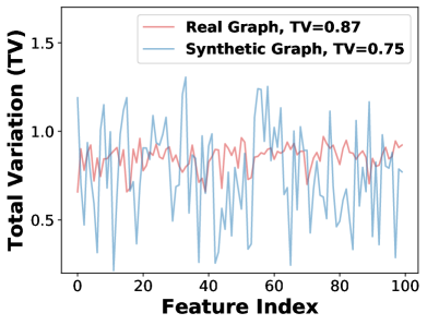
(a) Feature distributions of the real and low-frequency synthetic graphs

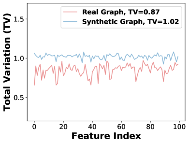
(b) Feature distributions of the real and high-frequency synthetic graphs

Figure 1. Visualization of the total variations in the synthetic graphs condensed by the low-pass and high-pass filters respectively. For clarity, we only visualize the first 100-dimensional node features. Best viewed in color.

To verify this analysis, we further perform a toy experiment, in which we use $\mathbf{AXW}$ and $\mathbf{LXW}$, representing the low-pass and high-pass filters (FAGCN), as the condensation models to learn the synthetic graphs of the Pubmed data. Subsequently, we compute the TVs of node features in the two synthetic graphs and present their visualizations in Figure 1. Notably, the average TV of the synthetic graph condensed by the high-pass filter (1.02) surpasses that of the real graph (0.87), whereas the inverse holds true for the low-pass filter (0.75). This observation shows that synthetic graphs generated by the low-pass filter will have smooth features, whereas the high-pass filter results in rougher results, supporting the aforementioned analysis that the condensation model will inject its spectrum bias into the synthetic graph.

Replacing the one-layer GCN with other graph filters results in different GNNs. For example, PPNP (PPNP) defines the filter as $g_{i}=\alpha+(1-\alpha)\lambda_{i}$, where $\alpha$ is a hyperparameter. This replacement does not affect our analysis but provides different spectrum preferences. On the other hand, despite the simplifications in our analysis, certain issues remain unaddressed. For instance, the impact of spectrum bias on the structure of synthetic graphs. We leave them for future investigations.

Remark 1.

(Motivation) In graph condensation, the usage of graph filters or GNNs biases the synthetic graph toward a specific spectrum, which cannot preserve the entire distribution of the real graph. To address this problem, it is important to avoid using the spectrum information during the condensation process.

4. The Proposed Method

In this section, we introduce the proposed method GCEM, as illustrated in Figure 2(c). Its condensation process can be divided into two steps: (1) Generate eigenbasis by matching node features within different subspaces. (2) Construct the synthetic graph by using the generated eigenbasis and the spectrum of the real graph.

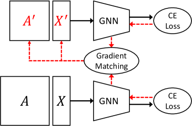
(a) Gradient matching on graphs

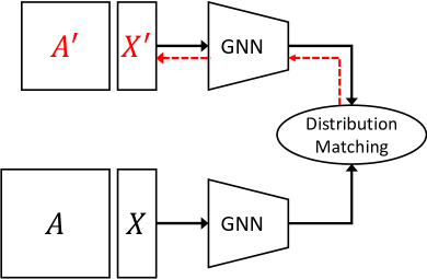
(b) Distribution matching on graphs

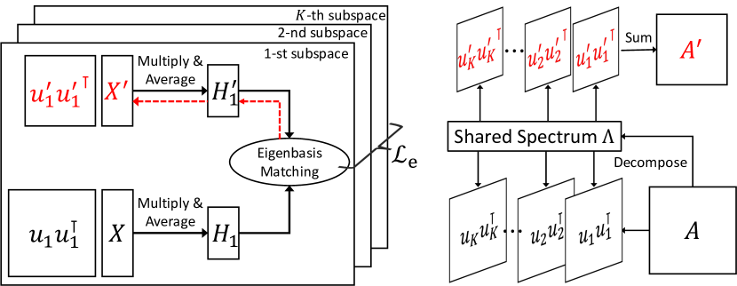
(c) Eigenbasis matching on graphs

Figure 2. Comparison between different graph condensation methods, where the red characters represent the synthetic data, the solid black lines, and red dotted lines indicate the forward and backward passes, respectively. (a) Gradient matching matches the model gradients of the Cross-Entropy (CE) loss. (b) Distribution matching matches the node representations learned by the condensation GNNs. (c) Eigenbasis matching first matches the node features in the subspaces defined by the eigenbasis, and then constructs the adjacency matrix by leveraging the spectrum of the real graph.

4.1. Pre-processing and Initialization

As explained in Section 3, avoiding the usage of spectrum information in the condensation process can eliminate the spectrum bias. However, both the adjacency matrix and graph Laplacian have their own inherent spectrum, which cannot be used directly. Therefore, we need to first pre-process the real graph and initialize the synthetic graph.

Pre-processing of real graph. Since the number of eigenvalues in the real graph is significantly greater than that in the synthetic graph, we can only match a few important eigenvectors. Specifically, we aim to choose the eigenvectors with the $K_{1}$ smallest and the $K_{2}$ largest eigenvalues, where $K_{1}$ and $K_{2}$ are hyperparameters, and $K_{1}+K_{2}\leq n^{\prime}$. This approach has been used in the graph coarsening algorithms (k1+k2), as they encode the important frequency information of the graphs. The selected eigenvectors form a new eigenbasis, which is denoted as $\mathbf{U}_{K}=[\mathbf{u}_{1},\cdots,\mathbf{u}_{K_{1}},\mathbf{u}_{n-K_{2}},\cdots,\mathbf{u}_{n}]\in\mathbb{R}^{n\times K}$.

Initialization of synthetic graph. Different from previous GC methods that directly learn the adjacency matrix of the synthetic graph, GCEM aims to generate its eigenbasis. To ensure that the initialized eigenbasis is valid, we first use the stochastic block model (SBM) to randomly generate the adjacency matrix of the synthetic graph $\mathbf{A}^{\prime}\in\{0,1\}^{n^{\prime}\times n^{\prime}}$, and then decompose it to produce the top-$K$ eigenvectors as the initialized eigenbasis $\mathbf{U}_{K}^{\prime}\in\mathbb{R}^{n^{\prime}\times K}$. Moreover, to initialize the synthetic node features $\mathbf{X}^{\prime}\in\mathbb{R}^{n^{\prime}\times d}$, we first train an MLP $\rho(\cdot)$ in the real node features. Then we freeze the well-trained MLP and feed the synthetic node features into it to minimize the classification objective. This process can be formulated as:

(10) $$\min_{\mathbf{X}^{\prime}}\sum_{i=1}^{n^{\prime}}-y_{i}^{\prime}\log\rho(\mathbf{x}_{i}^{\prime},\theta^{*}),\text{ s.t. }\theta^{*}=\underset{\theta}{\arg\min}\sum_{i=1}^{n}-y_{i}\log\rho(\mathbf{x}_{i},\theta)$$

where $\theta$ indicates the parameters of MLP.

4.2. Eigenbasis Matching

The subspaces, which are represented as the outer product of the eigenbasis, encode the fundamental structures of the graph. Eigenbasis matching aims to align the subspaces between the real and synthetic graphs, enabling knowledge transfer between the two graphs. However, the subspaces of real and synthetic graphs have different sizes and cannot be directly aligned. Therefore, we choose to match the node features in the subspaces as an alternative. Specifically, we first calculate the node representations learned in each subspace:

(11) $$\mathbf{H}_{k}=\mathbf{u}_{k}\mathbf{u}_{k}^{\top}\mathbf{X},\quad\mathbf{H}^{\prime}_{k}=\mathbf{u}^{\prime}_{k}{\mathbf{u}^{\prime}_{k}}^{\top}\mathbf{X}^{\prime},$$

where $\mathbf{H}_{k}$ and $\mathbf{H}^{\prime}_{k}$ represent the real and synthetic node features in the $k$-th subspace.

Subsequently, we average the representations of nodes belonging to the same class to learn the class-level representations:

(12) $$\overline{\mathbf{h}}_{c,k}=\frac{1}{|V_{c}|}\sum_{i\in V_{c}}\mathbf{h}_{i,k},\quad\overline{\mathbf{h}^{\prime}}_{c,k}=\frac{1}{|V^{\prime}_{c}|}\sum_{i\in V^{\prime}_{c}}\mathbf{h}^{\prime}_{i,k},$$

where $\mathbf{h}_{i,k}$ indicates the $i$-th row of $\mathbf{H}_{k}$, $V_{c}$ represents the nodes belonging to $c$-th class, and $\overline{\mathbf{h}}_{c,k}$ is the representation of $c$-th class center in $k$-th subspace. We omit the explanation of symbols in the synthetic graph for clarity.

The class-level representations describe the graph data distribution from both the subspace and category perspectives. Intuitively, aligning these representations will make the real and synthetic graphs share similar distributions:

(13) $$\mathcal{L}_{e}=\sum_{c=1}^{C}\sum_{k=1}^{K}\left\|\overline{\mathbf{h}}_{c,k}-\overline{\mathbf{h}^{\prime}}_{c,k}\right\|^{2},$$

where $C$ is the total number of classes. Notably, this matching function is also a distribution matching objective. The difference is that it treats different subspaces equally without using the spectral information to reweight the subspaces.

Additionally, as the basis of graph Fourier transform, eigenbasis is naturally normalized and orthogonal to each other. However, directly optimizing $\mathbf{U}_{K}^{\prime}$ via gradient descent cannot preserve such properties. Therefore, an additional regularization is used to constrain the representation space:

(14) $$\mathcal{L}_{o}=\left\|{\mathbf{U}_{K}^{\prime}}^{\top}\mathbf{U}_{K}^{\prime}-\mathbf{I}_{K}\right\|^{2}.$$

4.3. Discrimination Constraint

In practice, we find that only using eigenbasis matching does not achieve optimal performance, as it only considers the statistical mean of data representation and ignores the data variance. To address this problem, we employ a class-aware regularization technique (IDM; CAFE) to improve the discriminative power of the synthetic graph. Specifically, we aim to use the class-level representations of the synthetic graph as a classifier to categorize the nodes in the real graph. However, the node features in a single subspace are insufficient since they only capture a portion of the structural information. Therefore, we need to merge the node features from various subspaces:

(15) $$\overline{\mathbf{h}^{\prime}}_{c}=\sum_{k=1}^{K}(1-\lambda_{k})\overline{\mathbf{h}^{\prime}}_{c,k},\quad\overline{\mathbf{H}^{\prime}}=\left[\overline{\mathbf{h}^{\prime}}_{1},\overline{\mathbf{h}^{\prime}}_{2},\cdots,\overline{\mathbf{h}^{\prime}}_{C}\right]^{\top},$$

where $\lambda_{k}$ is the $k$-th eigenvalue of the real graph Laplacian, and $\overline{\mathbf{H}^{\prime}}\in\mathbb{R}^{d\times C}$ is the learned classifier. Finally, we use it to classify the training nodes in the real graph:

(16) $$\mathcal{L}_{d}=-\sum_{i=1}^{N}\sum_{j=1}^{C}\mathbf{Y}_{ij}\ln{\left(\mathbf{A}\mathbf{X}\overline{\mathbf{H}^{\prime}}\right)_{ij}},$$

where $\mathbf{A}\mathbf{X}\overline{\mathbf{H}^{\prime}}\in\mathbb{R}^{N\times C}$ are the logits for classification.

Note that the discrimination constraint introduces the spectrum information in the condensation process, which conflicts with the eigenbasis matching. However, we find that adjusting the weights of eigenbasis matching and discrimination constraint can balance the performance and generalization of the synthetic graph. Ablation studies can be seen in Section 6.4.

4.4. Final Objective and Graph Construction

In summary, the overall loss function of GCEM is formulated as the weighted sum of three regularization terms:

(17) $$\mathcal{L}_{total}=\mathcal{L}_{e}+\alpha\mathcal{L}_{o}+\beta\mathcal{L}_{d},$$

where $\alpha$ and $\beta$ are the hyperparameters. The pseudo algorithm of CGEM is presented in Appendix C.

Upon minimizing the total loss function, GCEM generates the eigenbasis and node features of the synthetic graph. However, this data remains incomplete and cannot be directly utilized for GNNs due to the absence of a graph spectrum. Essentially, the eigenvalues reflect the smoothness of the corresponding eigenvectors. If the eigenbasis of the real and synthetic graphs align well, they can share the same spectrum. As a result, the final adjacency matrix of the synthetic graph is constructed as

(18) $$\mathbf{A}^{\prime}=\sum_{k=1}^{K}(1-\lambda_{k})\mathbf{u}_{k}^{\prime}{\mathbf{u}_{k}^{\prime}}^{\top}.$$

Complexity. The complexity of eigenvalue decomposition is $\mathcal{O}(n^{3})$. However, given that we only utilize the $K$ smallest or largest eigenvalues, the complexity is reduced to $\mathcal{O}(Kn^{2})$. We neglect the computational cost associated with the synthetic graph as it is significantly smaller in scale. Consequently, the complexity of $\mathcal{L}_{e}$ and $\mathcal{L}_{d}$ is $\mathcal{O}(Knd)$ and $\mathcal{O}(n^{2}d+Cnd)$, respectively. As a result, the overall computational complexity of GCEM is $\mathcal{O}((K+d)n^{2}+(K+C)nd)$.

5. Theoretical Analysis

In this section, we give a theoretical analysis of the eigenbasis matching, which preserves the spectral similarity of the real graphs.

Definition 0.

(Spectral similarity (RS)) Suppose that there exists a positive constant $\epsilon$, such that for all $\mathbf{s}\in\mathbb{R}^{n\times 1}$,

(19) $$(1-\epsilon)\mathbf{s}^{\top}\mathbf{A}\mathbf{s}<\mathbf{s}^{\top}\mathbf{B}\mathbf{x}<(1+\epsilon)\mathbf{s}^{\top}\mathbf{A}\mathbf{s},$$

where the matrix $\mathbf{B}$ is the approximation of matrix $\mathbf{A}$.

In our context, it is impossible to compare the spectral similarity of the real and synthetic graphs with respect to a random signal, due to their difference in graph size. Therefore, we only consider the spectral similarity with respect to the node features:

(20) $$(1-\epsilon)\mathbf{x}^{\top}\mathbf{L}\mathbf{x}<{\mathbf{x}^{\prime}}^{\top}\mathbf{L}^{\prime}\mathbf{x}^{\prime}<(1+\epsilon)\mathbf{x}^{\top}\mathbf{L}\mathbf{x}.$$

If the above inequality holds, the synthetic graph Laplacian $\mathbf{L}^{\prime}$ approximates the spectrum of the real graph Laplacian $\mathbf{L}$.

Proposition 0.

The graph generated by GCEM is an $\epsilon$-spectral approximation of the real graph with respect to the node features.

Table 3. Node classification performance of different methods, mean accuracy (%) ± standard deviation. Bold indicates the best performance and underline means the runner-up. Results are taken from the original paper and - means the missing results.

Dataset	Ratio ($r$)	Traditional Methods				Graph Condensation Methods				Whole Dataset
		Random $(\mathbf{A}^{\prime},\mathbf{X}^{\prime})$	Coarsening $(\mathbf{A}^{\prime},\mathbf{X}^{\prime})$	Herding $(\mathbf{A}^{\prime},\mathbf{X}^{\prime})$	K-Center $(\mathbf{A}^{\prime},\mathbf{X}^{\prime})$	GCOND $(\mathbf{A}^{\prime},\mathbf{X}^{\prime})$	SFGC $(\mathbf{X}^{\prime})$	GCDM $(\mathbf{A}^{\prime},\mathbf{X}^{\prime})$	GCEM $(\mathbf{U}^{\prime},\mathbf{X}^{\prime})$
Cora	1.30%	63.6±3.7	31.2±0.2	67.0±1.3	64.0±2.3	79.8±1.3	80.1±0.4	69.4±1.3	80.9±1.1	81.2±0.2
	2.60%	72.8±1.1	65.2±0.6	73.4±1.0	73.2±1.2	80.1±0.6	81.7±0.5	77.2±0.4	81.9±0.5
	5.20%	76.8±0.1	70.6±0.1	76.8±0.1	76.7±0.1	79.3±0.3	81.6±0.8	79.4±0.1	81.9±0.9
Citeseer	0.90%	54.4±4.4	52.2±0.4	57.1±1.5	52.4±2.8	70.5±1.2	71.4±0.5	62.0±0.1	72.4±0.7	71.7±0.1
	1.80%	64.2±1.7	59.0±0.5	66.7±1.0	64.3±1.0	70.6±0.9	72.4±0.4	69.5±1.1	73.5±0.7
	3.60%	69.1±0.1	65.3±0.5	69.0±0.1	69.1±0.1	69.8±1.4	70.6±0.7	69.8±0.2	73.2±0.4
Pubmed	0.08%	69.4±0.2	76.7±0.7	64.5±2.7	18.1±0.1	76.5±0.2	-	75.7±0.3	77.8±1.0	79.3±0.2
	0.15%	73.3±0.7	76.2±0.5	69.4±0.7	28.7±4.1	77.1±0.5	-	77.3±0.1	78.3±1.3
	0.30%	77.8±0.3	78.0±0.5	78.2±0.4	42.8±4.1	77.9±0.4	-	78.3±0.3	78.3±0.7
arXiv	0.05%	47.1±3.9	35.4±0.3	52.4±1.8	47.2±3.0	61.3±0.5	65.5±0.7	-	64.3±0.6	71.4±0.1
	0.25%	57.3±1.1	43.5±0.2	58.6±1.2	56.8±0.8	64.2±0.4	66.1±0.4	59.6±0.4	65.5±0.6
	0.50%	60.0±0.9	50.4±0.1	60.4±0.8	60.3±0.4	63.1±0.5	66.8±0.4	62.4±0.1	65.5±0.5
Flickr	0.10%	41.8±2.0	41.9±0.2	42.5±1.8	42.0±0.7	45.9±0.1	46.6±0.2	46.8±0.2	50.3±0.3	47.2±0.1
	0.50%	44.0±0.4	44.5±0.1	43.9±0.9	43.2±0.1	45.0±0.2	47.0±0.1	47.9±0.3	50.2±0.2
	1.00%	44.6±0.2	44.6±0.1	44.4±0.6	44.1±0.4	45.0±0.1	47.1±0.1	47.5±0.1	50.1±0.2

Proof.

We first characterize the spectral similarity of node features in the real and synthetic graphs:

(21) $$\mathbf{x}^{\top}\mathbf{L}\mathbf{x} =\mathbf{x}^{\top}\sum_{k=1}^{n}\lambda_{k}\mathbf{u}_{k}\mathbf{u}_{k}^{\top}\mathbf{x}\approx\sum_{k=1}^{K}\lambda_{k}\mathbf{x}^{\top}\mathbf{u}_{k}\mathbf{u}_{k}^{\top}\mathbf{x},$$

(22) $${\mathbf{x}^{\prime}}^{\top}\mathbf{L}^{\prime}\mathbf{x}^{\prime} ={\mathbf{x}^{\prime}}^{\top}(\sum_{k=1}^{n^{\prime}}\lambda_{k}\mathbf{u}_{k}^{\prime}{\mathbf{u}_{k}^{\prime}}^{\top}+\tilde{\mathbf{U}}\bm{\Lambda}\tilde{\mathbf{U}}^{\top})\mathbf{x}^{\prime}\approx\sum_{k=1}^{K}\lambda_{k}{\mathbf{x}^{\prime}}^{\top}\mathbf{u}_{k}^{\prime}{\mathbf{u}_{k}^{\prime}}^{\top}\mathbf{x}^{\prime}+\Delta,$$

where $\tilde{\mathbf{U}}$ is the residual term associated with the non-orthogonality of the eigenbasis, and $\Delta={\mathbf{x}^{\prime}}^{\top}\tilde{\mathbf{U}}\bm{\Lambda}\tilde{\mathbf{U}}^{\top}\mathbf{x}^{\prime}$.

Next, we characterize the spectral similarity of a subspace $\mathbf{u}\mathbf{u}^{\top}$:

(23) $$\mathbf{x}^{\top}\mathbf{u}\mathbf{u}^{\top}\mathbf{x}=(\mathbf{u}\mathbf{u}^{\top}\mathbf{x})^{\top}(\mathbf{u}\mathbf{u}^{\top}\mathbf{x})=\|\mathbf{u}\mathbf{u}^{\top}\mathbf{x}\|_{2}^{2}.$$

We denote the absolute value of the difference in the total variations between the real and synthetic graphs as $\delta$. Combining Equations 21, 22, and 23, we have:

(24) $$\delta=\left|{\mathbf{x}^{\prime}}^{\top}\mathbf{L}^{\prime}\mathbf{x}^{\prime}-\mathbf{x}^{\top}\mathbf{L}\mathbf{x}\right| =\left|\sum_{k=1}^{K}\lambda_{k}||\mathbf{u}_{k}^{\prime}{\mathbf{u}_{k}^{\prime}}^{\top}\mathbf{x}^{\prime}||_{2}^{2}-\sum_{k=1}^{K}\lambda_{k}||\mathbf{u}_{k}\mathbf{u}_{k}^{\top}\mathbf{x}||_{2}^{2}+\Delta\right|$$

$$\leq\sum_{k=1}^{K}\lambda_{k}||\mathbf{u}_{k}^{\prime}{\mathbf{u}_{k}^{\prime}}^{\top}\mathbf{x}^{\prime}-\mathbf{u}_{k}\mathbf{u}_{k}^{\top}\mathbf{x}||_{2}^{2}+\left|\Delta\right|=\epsilon.$$

The above inequality shows that there is an upper bound on $\delta$ and the synthetic graph is a $\epsilon$-spectral approximation of the real graph. Notably, the first and second terms are related to $\mathcal{L}_{e}$ and $\mathcal{L}_{o}$. Optimizing the objective of GCEM will make the bound tighter. ∎

6. Experiments

In this section, we conduct experiments on a variety of graph datasets to verify the effectiveness and generalization of the proposed graph condensation method GCEM.

6.1. Experimental Setup

Datasets. To evaluate the effectiveness of our GCEM, we select five representative graph datasets, including three Planetoid datasets (GCN), OGB-arXiv (OGB), and Flickr (Flickr). See Appendix B for a detailed description of these datasets.

Baselines. We benchmark our model against seven competitive baselines, which can be divided into two categories: One is the traditional graph reduction methods, including three coreset methods, i.e., Random, Herding, and K-Center (core_set1; core_set2), and one coarsening method (coarsening1). Another is the graph condensation methods, including two gradient matching methods, i.e., GCOND (GCond) and SFGC (SFGC), and one distribution matching method, i.e., GCDM (GCDM).

Evaluation protocol. To fairly evaluate the quality of synthetic graphs, we perform the following two steps for all methods: (1) Condensation step, in which we apply the condensation methods to the training set of the real graphs. (2) Evaluation step, in which we train GNNs on the generated synthetic graph and then evaluate their performance on the test set of real graphs. In the effectiveness experiment conducted in Section 6.2, we use a two-layer GCN as both the condensation and evaluation model for all methods, suggested by the previous work (GCond; SFGC). In the generalization experiment presented in Section 6.3, we select seven representative GNNs, including three spatial GNNs, i.e., GCN (GCN), SGC (SGC), and PPNP (PPNP), and four spectral GNNs, i.e., ChebyNet (ChebNet), ChebyNetII (ChebNetII), BernNet (BernNet), and GPR-GNN (GPR-GNN). Notably, the hyperparameters of both condensation and evaluation models are searched based on the performance of the validation set in the real graphs.

Settings and hyperparameters. In the condensation step, for all datasets, we use the public data splits and run the condensation methods 10 times to generate 10 synthetic graphs for evaluation to eliminate randomness. Moreover, In the evaluation step, spatial GNNs have two aggregation layers and the polynomial order of spectral GNNs is set to 10. All GNNs have 256 hidden units. We use Adam as the optimizer. For more details, such as the compression ratio $r$, see Appendix D.

Table 4. Generalization performance of different methods across GNNs. $\uparrow$ means higher the better and $\downarrow$ means lower the better. Avg. and Var. indicate the average accuracy and variance of GNNs, respectively.

Datasets (Ratio)	Methods	Spatial GNNs			Spectral GNNs				Avg. ($\uparrow$)	Var. ($\downarrow$)
		GCN	SGC	PPNP	ChebyNet	ChebyNetII	BernNet	GPR-GNN
Cora ($r=2.60\%$)	GCOND	80.1	79.3	78.5	76.0	70.4	73.6	77.2	76.44	10.16
	SFGC	81.1	79.1	78.8	79.0	79.2	80.0	82.2	79.91	1.41
	GCEM	81.9	79.8	81.4	81.4	80.7	80.8	82.3	81.19	0.59
Citeseer ($r=1.80\%$)	GCOND	70.5	70.3	69.6	68.3	64.9	63.1	67.2	67.70	6.83
	SFGC	71.6	71.8	70.5	71.8	71.2	71.1	71.7	71.38	0.20
	GCEM	73.5	72.3	73.1	72.7	73.6	72.6	73.1	72.98	0.20
Pubmed ($r=0.15\%$)	GCOND	77.7	77.6	77.3	76.0	75.3	74.4	76.5	76.40	1.33
	SFGC	77.5	77.4	77.6	77.3	76.8	76.4	78.6	77.37	0.41
	GCEM	78.3	77.3	78.2	78.0	78.3	77.2	79.0	78.04	0.33
arXiv ($r=0.25\%$)	GCOND	63.2	63.7	63.4	54.9	55.1	55.0	60.5	59.40	15.46
	SFGC	65.1	64.8	63.9	60.7	62.4	63.8	64.9	63.66	2.19
	GCEM	65.5	64.6	65.1	65.3	64.5	64.5	66.0	65.07	0.28
Flickr ($r=0.50\%$)	GCOND	47.1	46.1	45.9	42.8	43.3	44.3	46.4	45.13	2.36
	SFGC	47.1	42.5	40.7	45.4	44.9	45.7	46.4	44.67	4.43
	GCEM	50.2	50.7	49.9	49.6	50.3	50.4	50.1	50.17	0.11

6.2. Node Classification

The node classification performance is reported in Table 3, in which we have the following observations:

First, the graph condensation methods consistently outperform the traditional methods, including coreset and coarsening. The reasons are two-fold: On the one hand, graph condensation methods can leverage the powerful representation learning ability of GNNs to generate graph data. On the other hand, the condensation process involves the downstream task information, i.e., categories, which better captures the distribution of the real graphs. In contrast, the traditional methods can only leverage the structural information.

Second, GCEM achieves state-of-the-art performance in four of five graph datasets, demonstrating its effectiveness in preserving the distribution of real graphs. Generally, existing graph condensations heavily rely on the spectrum preferences of GNNs to generate synthetic graphs. However, the results of GCEM reveal that spectrum-free condensation can also learn good synthetic graphs. Furthermore, some results of GCEM are better than those on the entire dataset, which may be due to the use of high-frequency information, e.g., eigenvectors with larger eigenvalues.

Third, the performance of GCEM is slightly lower than SFGC in the arXiv dataset. The reason is that arXiv is the largest dataset in our experiments, which has nearly 0.17M nodes. Under the compression ratios of 0.05% - 0.50%, there are only hundreds of eigenvectors for eigenbasis matching, which cannot cover all the important subspaces, leading to performance degradation.

6.3. Generalization on Different Architectures

In this section, we evaluate the generalization of the synthetic graphs generated by different graph condensation methods. In particular, we report the average accuracy and variance of seven GNNs to reflect their performance gaps. Results are shown in Table 4, from which we can see the following discoveries:

First, GCEM stands out by exhibiting the highest average node classification accuracy across all datasets, compared to GCOND and SFGC, indicating that the synthetic graphs generated by GCEM can consistently benefit a variety of GNNs. Moreover, in contrast to GCOND, GCEM significantly reduces the performance gap between different GNNs. To illustrate, the variance of GCOND is 4-55 times higher than that of GCEM. On the other hand, SFGC also reduces the variance by adopting structure-free condensation but is still higher than that of GCEM. Additionally, here we do not report the performance of GCDM (GCDM) due to the lack of open-source code.

Second, comparing the generalization results of the two gradient matching methods, i.e., GCOND and SFGC, we can find that compressing the graph structure into node features can narrow the performance gap between different GNNs. However, this approach is less suitable for spectral GNNs, because it treats the identity matrix as the adjacency matrix. Generally, spectral GNNs are designed to learn the coefficients associated with different orders of the adjacency matrix (GPR-GNN; BernNet). Unfortunately, training on the identity matrix does not facilitate the acquisition of valuable coefficients.

Table 5. Ablation studies on Cora.

Cora	GCN ($\uparrow$)	ChebyNetII ($\uparrow$)	Avg. ($\uparrow$)	Var. ($\downarrow$)
GCEM	81.9	80.7	81.19	0.59
w/o $\mathcal{L}_{e}$	79.5	72.5	76.74	10.01
w/o $\mathcal{L}_{o}$	77.2	74.6	76.71	1.82
w/o $\mathcal{L}_{d}$	77.5	77.8	76.99	0.86

Table 6. Ablation studies on Pubmed.

Pubmed	GCN ($\uparrow$)	ChebyNetII ($\uparrow$)	Avg. ($\uparrow$)	Var. ($\downarrow$)
GCEM	78.3	78.3	78.04	0.33
w/o $\mathcal{L}_{e}$	77.1	75.6	76.46	2.02
w/o $\mathcal{L}_{o}$	77.6	74.9	77.37	1.48
w/o $\mathcal{L}_{d}$	77.8	77.4	77.73	0.28

6.4. Ablation Study

We perform ablation studies in the Cora and Pubmed datasets to verify the effectiveness of different regularization terms, i.e., $\mathcal{L}_{e}$, $\mathcal{L}_{o}$, and $\mathcal{L}_{d}$. The results are reported in Tables 5 and 6.

First of all, it is evident that all these regularization terms contribute to both the effectiveness and generalization of GCEM. Removing any of them will affect the model’s performance. Moreover, it is worth noting that $\mathcal{L}_{e}$ primarily governs the generalization ability of GCEM, as the variance of GNNs increases significantly when this term is omitted. Next, $\mathcal{L}_{o}$ also plays a vital role in learning valuable synthetic graphs, as it preserves the orthogonality of eigenbasis. Removing this term will degenerate both the effectiveness and generalization of GCEM. Finally, we observe that $\mathcal{L}_{o}$ mainly affects the performance of GCEM rather than the generalization ability, because the variance remains basically unchanged after removing this term. To dive into the detailed results, see Appendix E.

6.5. Visualization

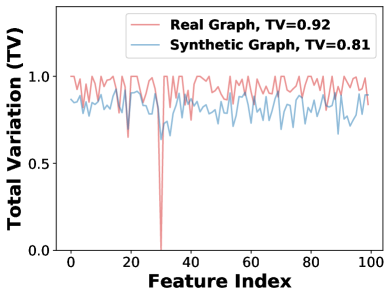
(a) Epoch 0: $\delta$=0.15, Acc=31.8

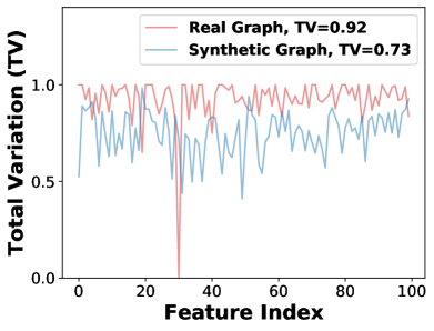
(b) Epoch 100: $\delta$=0.22, Acc=78.0

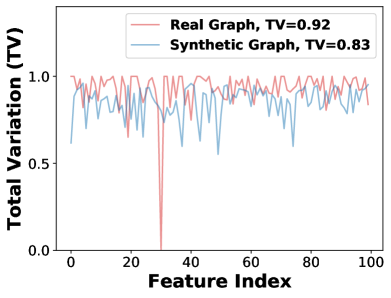
(c) Epoch 150: $\delta$=0.15, Acc=79.3

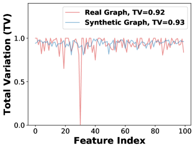
(d) Epoch: 200: $\delta$=0.08, Acc=79.8

Figure 3. Visualization of the total variations of the synthetic graphs in different training epochs, where $\delta=\left|{\mathbf{x}^{\prime}}^{\top}\mathbf{L}^{\prime}\mathbf{x}^{\prime}-\mathbf{x}^{\top}\mathbf{L}\mathbf{x}\right|$ reflects the difference in total variation, and Acc means accuracy in percent.

In Figure 3, we visualize how the total variation of the synthetic graph evolves during the training process on the Cora dataset. Specifically, Figure 3(a) illustrates the signal distribution at the first epoch, which has a lower classification accuracy due to random initialization. An interesting phenomenon emerges in Figures 3(b) and 3(c), where the total variations of the synthetic graphs at epochs 150 and 200 become smaller than the random initialization. Simultaneously, their performance notably improves. We guess this is because GCEM will first align the low-frequency subspaces of the real and synthetic graphs, which reduces the total variation and improves the model performance. Finally, we find that the synthetic graph at Epoch 200 demonstrates the best performance. It not only has the highest classification accuracy but also closely matches the signal distributions in the real graphs. This experiment validates Proposition 2 that optimizing the objective of GCEM will reduce the difference in total variation.

6.6. Time and Space Overhead

In this section, we compare the time and space overhead of different graph condensation methods. Specifically, we evaluate the time costs associated with both the pre-processing and condensation stages, as well as the memory usage. The results are shown in Table 7. It can be seen that GCOND has minimal pre-processing time costs and memory usage. But its bi-level optimization results in maximum training time. SFGC spends a lot of time in the pre-processing stage because it needs to pre-calculate the training trajectory of GNNs. On the contrary, GCEM leverages the advantages of distribution match, which significantly reduces the model complexity.

Table 7. Time and space overhead of different methods

	Pre-processing (s)	Condensation (s)	Memory (MB)
GCOND	2.29	638.25	957
SFGC	1803.16	539.22	1261
GCEM	19.27	10.14	1317

7. Related Work

Graph Neural Networks aim to design effective convolution operators to exploit the node features and topology structure information adequately. Existing methods are roughly divided into spatial and spectral approaches. Spatial GNNs focus on the neighbor aggregation strategies in the vertical domain (GCN; GAT; SAGE). Spectral GNNs aim to design filters in the spectral domain to extract certain frequencies for the downstream tasks (GPR-GNN; ChebNet; Specformer; ChebNetII; BernNet).

Dataset Condensation, a.k.a., dataset distillation, has shown great potential in reducing data redundancy and accelerating model training (dd_survey1; dd_survey2; dd_survey3; dd_survey4). Dataset condensation (DC) aims to generate small yet informative synthetic training data by matching the model gradient (DCGM; DDMTT; HaBa) or data distribution (DCDM; CAFE) between the real and synthetic data. As a result, models trained on the real and synthetic data will have comparable performance.

DC has been widely used for graph data, known as graph condensation. Existing methods include models for node-level tasks, e.g., GCond (GCond), SFGC (SFGC), GCDM (GCDM) and MCond (MCond), and graph-level tasks, e.g., DosCond (DosCond) and KIDD (KIDD). GCond is the first graph condensation method based on gradient matching, which needs to optimize GNNs during the condensation procedure, resulting in inefficient computation. DosCond further provides one-step gradient matching to approximate the first step of gradient matching, thereby avoiding the bi-level optimization. GCDM proposes distribution matching for graph condensation, which views the receptive fields of a graph as its distribution. Additionally, SFGC proposes structure-free graph condensation to compress the structural information into the node features. KIDD utilizes the kernel ridge regression to further reduce the computational cost. However, all these methods do not consider the influence of GNNs, which may achieve sub-optimal performance. In contrast, GCEM provides a way to get rid of the effect of specific GNNs.

8. Conclusion

In this paper, we study the generalization ability of graph condensation methods. Surprisingly, we observe that GNNs will inject their spectrum bias into the synthetic graph, resulting in poor generalization. To address this issue, we propose graph condensation via eigenbasis matching, which aligns the eigenbasis of the real and synthetic graphs to get rid of the influence of GNNs. Extensive experiments on the node classification task validate both the effectiveness and generalization of the proposed method. A promising future work is to explore eigenbasis matching without the need for explicit eigenvalue decomposition.

Appendix A Setup of Investigation

A.1. Condensation Step

We use lr, wd, and dropout to denote the learning rate, weight decay and dropout for the Spatial GNNs and the linear layer of the Spectral GNNs, and use $\text{lr}_{p}$, $\text{wd}_{p}$ and $\text{dropout}_{p}$ for the propagation layer of the Spectral GNNS, respectively. And $K$ indicates the step of the propagation for PPNP and Spectral GNNs. During the condensation procedure, we fix 400 epochs to condense the graphs. The hyper-parameters and models’ settings are listed in Table 8.

Table 8. The hyper-parameters of models during the condensation step.

GNNs	Hyper-parameters
SGC	layers=2, lr=0.01, wd=0.0, dropout=0.5
GCN	layers=2, hidden=64, lr=0.01, wd=0.0, dropout=0.5
PPNP	linear layers=1, $K$=2, lr=0.01, wd=0.0, dropout=0.5
ChebyNet	linear layers=1, $K$=10, lr=0.01, $\text{lr}_{p}$=0.01, wd=0.0, $\text{wd}_{p}$=0.0, dropout=0.5, $\text{dropout}_{p}$=0.5
BernNet	linear layers=1, $K$=10, lr=0.01, $\text{lr}_{p}$=0.01, wd=0.0, $\text{wd}_{p}$=0.0, dropout=0.5, $\text{dropout}_{p}$=0.5
GPR-GNN	linear layers=1, $K$=10, lr=0.01, $\text{lr}_{p}$=0.01, wd=0.0, $\text{wd}_{p}$=0.0, dropout=0.5, $\text{dropout}_{p}$=0.5

A.2. Evaluation Step

We train six GNNs in the condensed graphs with 600 epochs. The hyper-parameters and settings are listed in Table 9.

Table 9. The hyper-parameters of models during the evaluation step.

GNNs	Hyper-parameters
SGC	layers=2, lr=0.01, wd=0.0005, dropout=0.5
GCN	layers=2, hidden=64, lr=0.01, wd=0.0005, dropout=0.5
PPNP	linear layers=2, hidden=64, $K$=2, lr=0.01, wd=0.0005, dropout=0.5
ChebyNet	linear layers=2, hidden=64, $K$=10, lr=0.005, $\text{lr}_{p}$=0.01, wd=0.0005, $\text{wd}_{p}$=0.0, dropout=0.5, $\text{dropout}_{p}$=0.5
BernNet	linear layers=2, hidden=64, $K$=10, lr=0.01, $\text{lr}_{p}$=0.01, wd=0.0005, $\text{wd}_{p}$=0.0, dropout=0.5, $\text{dropout}_{p}$=0.5
GPR-GNN	linear layers=2, hidden=64, $K$=10, lr=0.01, $\text{lr}_{p}$=0.01, wd=0.0005, $\text{wd}_{p}$=0.0, dropout=0.5, $\text{dropout}_{p}$=0.5

Appendix B Statistics of Graph Datasets

Table 10 describes node numbers, edge numbers, class numbers, feature dimensions, and node numbers of the largest connected component (LCC) of the datasets. On real-world datasets, there are many isolated nodes in the graphs that may influence the performance of the condensed graphs. So we condense the synthetic graphs on the largest connected graphs of the original datasets.

Table 10. Statistics of datasets.

Datasets	Nodes	Edges	Classes	Features	LCC
Cora	2,708	5,429	7	1,433	2,485
Citeseer	3,327	4,732	6	3,703	2,120
Pubmed	19,717	44,338	3	500	19,717
arXiv	169,343	1,166,243	40	128	169,343
Flickr	89,250	899,756	7	500	89,250

Appendix C Pseudo Algorithm

The pseudo algorithm of GCEM is shown below.

1 Input: Training data $\mathcal{T}=\left(\mathbf{A},\mathbf{X},\mathbf{Y}\right)$, pre-defined condensed labels $\mathbf{Y}^{\prime}$, pre-computed class-level representations of the real graph $\overline{\mathbf{h}}_{c,k}$ through Eq 12

2 Initialize synthetic node features $\mathbf{X}^{\prime}$ and synthetic eigenbasis $\mathbf{U}_{K}^{\prime}$ through Eq 10

3 for $t=0,...T-1$ do

4       Compute $\mathbf{H}^{\prime}_{k}=\mathbf{u}^{\prime}_{k}{\mathbf{u}^{\prime}_{k}}^{\top}\mathbf{X}^{\prime}$ and $\overline{\mathbf{h}^{\prime}}_{c,k}=\frac{1}{|V^{\prime}_{c}|}\sum_{i\in V^{\prime}_{c}}\mathbf{h}^{\prime}_{i,k}$

5       Compute the learned classifier $\overline{\mathbf{H}^{\prime}}$

6       Compute $\mathcal{L}_{e}=\sum_{c=1}^{C}\sum_{k=1}^{K}\left\|\overline{\mathbf{h}}_{c,k}-\overline{\mathbf{h}^{\prime}}_{c,k}\right\|^{2}$, $\mathcal{L}_{o}=\left\|{\mathbf{U}_{K}^{\prime}}^{\top}\mathbf{U}_{K}^{\prime}-\mathbf{I}_{K}\right\|^{2}$, and $\mathcal{L}_{d}=-\sum_{i=1}^{N}\sum_{j=1}^{C}\mathbf{Y}_{ij}\ln{\left(\mathbf{A}\mathbf{X}\overline{\mathbf{H}^{\prime}}\right)_{ij}}$

7       Optimize $\mathcal{L}_{total}=\mathcal{L}_{e}+\alpha\mathcal{L}_{o}+\beta\mathcal{L}_{d}$

8       if $t\%(\tau_{1}+\tau_{2})<\tau_{1}$ then

9             Update $\mathbf{U}_{K}^{\prime}\leftarrow\mathbf{U}_{K}^{\prime}-\eta_{1}\nabla_{\mathbf{U}_{K}^{\prime}}\mathcal{L}_{total}$

10      else

11             Update $\mathbf{X}^{\prime}\leftarrow\mathbf{X}^{\prime}-\eta_{2}\nabla_{\mathbf{X}^{\prime}}\mathcal{L}_{total}$

12       end if

13      

14 end for

15Compute $\mathbf{A}^{\prime}=\sum_{k=1}^{K}(1-\lambda_{k})\mathbf{u}_{k}^{\prime}{\mathbf{u}_{k}^{\prime}}^{\top}$

return $\mathbf{A}^{\prime}$, $\mathbf{X}^{\prime}$

Algorithm 1 GCEM for Graph Condensation

Appendix D Details in the experiment

D.1. Compression Ratio

We set the same compression ratio as GCond. For Cora, Citeseer and Pubmed, we set $r^{\prime}$ to be $\left\{25\%,50\%,100\%\right\}$ of the labeling rate $r_{y}$. For arXiv and Flickr, we set $r^{\prime}$ to be $\left\{0.1\%,0.5\%,1.0\%\right\}$ of $r_{y}$. Thus, node numbers of synthetic graphs $n^{\prime}$ are $n^{\prime}=r^{\prime}\times r_{y}\times n$. Condensation ratio $r$ is defined as $r=\frac{n^{\prime}}{n}$. Finally, we choose $r=\left\{1.30\%,2.60\%,5.20\%\right\}$ for Cora, $r=\left\{0.90\%,1.80\%,3.60\%\right\}$ for Citeseer, $r=\left\{0.08\%,0.15\%,0.30\%\right\}$ for Pubmed, $r=\left\{0.05\%,0.25\%,0.50\%\right\}$ for arXiv, and $r=\left\{0.10\%,0.50\%,1.00\%\right\}$ for Flickr.

D.2. Hyperparameters

The Table 11 shows the hyper-parameters of GCEM.

Table 11. The hyper-parameters of GCEM

Datasets	Ratio	epochs	k_ratio	$\tau_{1}$	$\tau_{2}$	$\alpha$	$\beta$	lr_feat	lr_eigenvecs	wd_feat	wd_eigenvec
Cora	1.30%	1000	1.00	5	15	0.5	1.0	0.0003	0.0005	0.05	0.05
	2.60%	1500	0.90	20	20	0.05	1.0	0.005	0.01	0.01	0.005
	5.20%	500	0.95	10	20	0.5	1.0	0.0003	0.00005	0.05	0.05
Citeseer	0.90%	2000	1.00	5	10	1.0	1.0	0.005	0.005	0.05	0.0
	1.80%	2000	1.00	5	10	1.0	1.0	0.005	0.005	0.05	0.0
	3.60%	2000	0.85	10	5	0.5	1.0	0.03	0.001	0.01	0.0
Pubmed	0.08%	1500	1.00	10	10	50.0	0.5	0.00001	0.0003	0.001	0.001
	0.15%	1500	1.00	10	7	50.0	0.5	0.00001	0.0005	0.005	0.00001
	0.30%	1500	1.00	10	7	50.0	0.5	0.00001	0.0003	0.005	0.005
arXiv	0.05%	2000	1.00	1	7	5.0	100.0	0.0001	0.00001	0.0005	0.01
	0.25%	2000	0.90	3	10	5.0	100.0	0.0005	0.00001	0.00005	0.01
	0.50%	2000	0.90	3	10	5.0	100.0	0.0005	0.00001	0.00005	0.01
Flickr	0.10%	2000	0.85	3	10	1.0	50.0	0.001	0.00001	0.0005	0.005
	0.50%	2000	0.85	3	10	1.0	50.0	0.001	0.00001	0.0005	0.005
	1.00%	2000	0.85	3	10	1.0	50.0	0.001	0.00001	0.0005	0.005

Appendix E Additional Experimental Results

Table 12 shows the generalization ability of ablation studies on Cora and Pubmed.

Table 12. Detailed ablation studies on Cora and Pubmed.

Datasets (Ratio)	Methods	Linear GNNs			Polynomial GNNs				Avg. ($\uparrow$)	Var. ($\downarrow$)
		GCN	SGC	PPNP	ChebyNet	ChebyNetII	BernNet	GPR-GNN
Cora ($r=2.60\%$)	GCEM	81.9	79.8	81.4	81.4	80.7	80.8	82.3	81.19	0.59
	w/o $\mathcal{L}_{e}$	79.5	71.3	78.6	78.8	72.5	77.1	79.4	76.74	10.01
	w/o $\mathcal{L}_{o}$	77.2	76.4	77.8	77.0	74.6	75.2	78.8	76.71	1.82
	w/o $\mathcal{L}_{d}$	77.5	74.9	77.5	76.9	77.8	76.7	77.6	76.99	0.86
Pubmed ($r=0.15\%$)	GCEM	78.3	77.3	78.2	78.0	78.3	77.2	79.0	78.04	0.33
	w/o $\mathcal{L}_{e}$	77.1	73.4	77.9	76.8	75.6	77.6	76.8	76.46	2.02
	w/o $\mathcal{L}_{o}$	77.6	77.1	77.7	78.1	74.9	77.0	79.2	77.37	1.48
	w/o $\mathcal{L}_{d}$	77.8	77.0	78.1	78.5	77.4	77.1	78.2	77.73	0.28

References

- (1)
- Bo et al. (2023a) Deyu Bo, Chuan Shi, Lele Wang, and Renjie Liao. 2023a. Specformer: Spectral Graph Neural Networks Meet Transformers. In ICLR.
- Bo et al. (2023b) Deyu Bo, Xiao Wang, Yang Liu, Yuan Fang, Yawen Li, and Chuan Shi. 2023b. A Survey on Spectral Graph Neural Networks. ArXiv abs/2302.05631 (2023).
- Bo et al. (2021) Deyu Bo, Xiao Wang, Chuan Shi, and Huawei Shen. 2021. Beyond Low-frequency Information in Graph Convolutional Networks. In AAAI. AAAI Press, 3950–3957.
- Cazenavette et al. (2022) George Cazenavette, Tongzhou Wang, Antonio Torralba, Alexei A. Efros, and Jun-Yan Zhu. 2022. Dataset Distillation by Matching Training Trajectories. In CVPR. IEEE, 10708–10717.
- Chien et al. (2021) Eli Chien, Jianhao Peng, Pan Li, and Olgica Milenkovic. 2021. Adaptive Universal Generalized PageRank Graph Neural Network. In ICLR. OpenReview.net.
- Chung (1997) Fan RK Chung. 1997. Spectral graph theory. Vol. 92. American Mathematical Soc.
- Defferrard et al. (2016) Michaël Defferrard, Xavier Bresson, and Pierre Vandergheynst. 2016. Convolutional Neural Networks on Graphs with Fast Localized Spectral Filtering. In NIPS. 3837–3845.
- Gao et al. (2023) Xin Gao, Tong Chen, Yilong Zang, Wentao Zhang, Quoc Viet Hung Nguyen, Kai Zheng, and Hongzhi Yin. 2023. Graph Condensation for Inductive Node Representation Learning. ArXiv abs/2307.15967 (2023).
- Geng et al. (2023) Jiahui Geng, Zongxiong Chen, Yuandou Wang, Herbert Woisetschlaeger, Sonja Schimmler, Ruben Mayer, Zhiming Zhao, and Chunming Rong. 2023. A Survey on Dataset Distillation: Approaches, Applications and Future Directions. In IJCAI. ijcai.org, 6610–6618.
- Hamedani et al. (2023a) Masoud Reyhani Hamedani, Jin-Su Ryu, and Sang-Wook Kim. 2023a. GELTOR: A Graph Embedding Method based on Listwise Learning to Rank. In WWW. ACM, 6–16.
- Hamedani et al. (2023b) Masoud Reyhani Hamedani, Jin-Su Ryu, and Sang-Wook Kim. 2023b. GELTOR: A Graph Embedding Method based on Listwise Learning to Rank. In WWW. ACM, 6–16.
- Hamilton et al. (2017) William L. Hamilton, Zhitao Ying, and Jure Leskovec. 2017. Inductive Representation Learning on Large Graphs. In NIPS. 1024–1034.
- Hansen and Bianchi (2023) Jonas Berg Hansen and Filippo Maria Bianchi. 2023. Total Variation Graph Neural Networks. In ICML, Vol. 202. PMLR, 12445–12468.
- He et al. (2021) Mingguo He, Zhewei Wei, Zengfeng Huang, and Hongteng Xu. 2021. BernNet: Learning Arbitrary Graph Spectral Filters via Bernstein Approximation. In NeurIPS. 14239–14251.
- He et al. (2022) Mingguo He, Zhewei Wei, and Ji-Rong Wen. 2022. Convolutional Neural Networks on Graphs with Chebyshev Approximation, Revisited. In NeurIPS.
- Hu et al. (2020) Weihua Hu, Matthias Fey, Marinka Zitnik, Yuxiao Dong, Hongyu Ren, Bowen Liu, Michele Catasta, and Jure Leskovec. 2020. Open Graph Benchmark: Datasets for Machine Learning on Graphs. In NeurIPS.
- Huang et al. (2021) Zengfeng Huang, Shengzhong Zhang, Chong Xi, Tang Liu, and Min Zhou. 2021. Scaling Up Graph Neural Networks Via Graph Coarsening. In KDD. ACM, 675–684.
- Jin et al. (2022a) Wei Jin, Xianfeng Tang, Haoming Jiang, Zheng Li, Danqing Zhang, Jiliang Tang, and Bing Yin. 2022a. Condensing Graphs via One-Step Gradient Matching. In KDD. 720–730.
- Jin et al. (2022b) Wei Jin, Lingxiao Zhao, Shichang Zhang, Yozen Liu, Jiliang Tang, and Neil Shah. 2022b. Graph Condensation for Graph Neural Networks. In ICLR.
- Jin et al. (2020) Yu Jin, Andreas Loukas, and Joseph F. JáJá. 2020. Graph Coarsening with Preserved Spectral Properties. In AISTATS, Vol. 108. PMLR, 4452–4462.
- Kipf and Welling (2017) Thomas N. Kipf and Max Welling. 2017. Semi-Supervised Classification with Graph Convolutional Networks. In ICLR. OpenReview.net.
- Klicpera et al. (2019) Johannes Klicpera, Aleksandar Bojchevski, and Stephan Günnemann. 2019. Predict then Propagate: Graph Neural Networks meet Personalized PageRank. In ICLR. OpenReview.net.
- Lei and Tao (2023) Shiye Lei and Dacheng Tao. 2023. A Comprehensive Survey of Dataset Distillation. ArXiv abs/2301.05603.
- Liu et al. (2022a) Mengyang Liu, Shanchuan Li, Xinshi Chen, and Le Song. 2022a. Graph Condensation via Receptive Field Distribution Matching. ArXiv abs/2206.13697 (2022).
- Liu et al. (2022b) Songhua Liu, Kai Wang, Xingyi Yang, Jingwen Ye, and Xinchao Wang. 2022b. Dataset Distillation via Factorization. In NeurIPS.
- Loukas (2019) Andreas Loukas. 2019. Graph Reduction with Spectral and Cut Guarantees. J. Mach. Learn. Res. 20 (2019), 116:1–116:42.
- Martinkus et al. (2022) Karolis Martinkus, Andreas Loukas, Nathanaël Perraudin, and Roger Wattenhofer. 2022. SPECTRE: Spectral Conditioning Helps to Overcome the Expressivity Limits of One-shot Graph Generators. In ICML, Vol. 162. PMLR, 15159–15179.
- NT and Maehara (2019) Hoang NT and Takanori Maehara. 2019. Revisiting Graph Neural Networks: All We Have is Low-Pass Filters. ArXiv abs/1905.09550 (2019).
- Quan et al. (2023) Yuhan Quan, Jingtao Ding, Chen Gao, Lingling Yi, Depeng Jin, and Yong Li. 2023. Robust Preference-Guided Denoising for Graph based Social Recommendation. In WWW. ACM, 1097–1108.
- Sachdeva and McAuley (2023) Noveen Sachdeva and Julian McAuley. 2023. Data Distillation: A Survey. ArXiv abs/2301.04272 (2023).
- Sener and Savarese (2018) Ozan Sener and Silvio Savarese. 2018. Active Learning for Convolutional Neural Networks: A Core-Set Approach. In ICLR. OpenReview.net.
- Shuman et al. (2013) David I. Shuman, Sunil K. Narang, Pascal Frossard, Antonio Ortega, and Pierre Vandergheynst. 2013. The Emerging Field of Signal Processing on Graphs: Extending High-Dimensional Data Analysis to Networks and Other Irregular Domains. IEEE Signal Process. Mag. 30, 3 (2013), 83–98.
- Spielman and Srivastava (2011) Daniel A. Spielman and Nikhil Srivastava. 2011. Graph Sparsification by Effective Resistances. SIAM J. Comput. 40, 6 (2011), 1913–1926.
- Velickovic et al. (2018) Petar Velickovic, Guillem Cucurull, Arantxa Casanova, Adriana Romero, Pietro Liò, and Yoshua Bengio. 2018. Graph Attention Networks. In ICLR.
- Wang et al. (2022) Kai Wang, Bo Zhao, Xiangyu Peng, Zheng Zhu, Shuo Yang, Shuo Wang, Guan Huang, Hakan Bilen, Xinchao Wang, and Yang You. 2022. CAFE: Learning to Condense Dataset by Aligning Features. In CVPR. IEEE, 12186–12195.
- Welling (2009) Max Welling. 2009. Herding dynamical weights to learn. In ICML, Vol. 382. ACM, 1121–1128.
- Wu et al. (2019) Felix Wu, Amauri H. Souza Jr., Tianyi Zhang, Christopher Fifty, Tao Yu, and Kilian Q. Weinberger. 2019. Simplifying Graph Convolutional Networks. In ICML, Vol. 97. PMLR, 6861–6871.
- Xu et al. (2023) Zhe Xu, Yuzhong Chen, Menghai Pan, Huiyuan Chen, Mahashweta Das, Hao Yang, and Hanghang Tong. 2023. Kernel Ridge Regression-Based Graph Dataset Distillation. In KDD. 2850–2861.
- Yu et al. (2023) Ruonan Yu, Songhua Liu, and Xinchao Wang. 2023. Dataset Distillation: A Comprehensive Review. ArXiv abs/2301.07014 (2023).
- Zeng et al. (2020) Hanqing Zeng, Hongkuan Zhou, Ajitesh Srivastava, Rajgopal Kannan, and Viktor K. Prasanna. 2020. GraphSAINT: Graph Sampling Based Inductive Learning Method. In ICLR. OpenReview.net.
- Zhao and Bilen (2023) Bo Zhao and Hakan Bilen. 2023. Dataset Condensation with Distribution Matching. In WACV. IEEE, 6503–6512.
- Zhao et al. (2021) Bo Zhao, Konda Reddy Mopuri, and Hakan Bilen. 2021. Dataset Condensation with Gradient Matching. In ICLR. OpenReview.net.
- Zhao et al. (2023) Ganlong Zhao, Guanbin Li, Yipeng Qin, and Yizhou Yu. 2023. Improved Distribution Matching for Dataset Condensation. In CVPR. IEEE, 7856–7865.
- Zheng et al. (2023) Xin Zheng, Miao Zhang, Chunyang Chen, Quoc Viet Hung Nguyen, Xingquan Zhu, and Shirui Pan. 2023. Structure-free Graph Condensation: From Large-scale Graphs to Condensed Graph-free Data. ArXiv abs/2306.02664 (2023).
- Zhu et al. (2021) Meiqi Zhu, Xiao Wang, Chuan Shi, Houye Ji, and Peng Cui. 2021. Interpreting and Unifying Graph Neural Networks with An Optimization Framework. In WWW. ACM / IW3C2, 1215–1226.