A generalization of the rational rough Heston approximation
Abstract
Previously, in [GR19], we derived a rational approximation of the solution of the rough Heston fractional ODE in the special case , which corresponds to a pure power-law kernel. In this paper we extend this solution to the general case of the Mittag-Leffler kernel with . We provide numerical evidence of the convergence of the solution.
1 Introduction
In the case , the rough Heston model of [JR16] may be written in forward variance form (see [GKR19]) as
| (1.1) |
where is the forward variance curve, , and the kernel is given by
where denotes the generalized Mittag-Leffler function.
Let and . According to [GKR19], the forward variance model (1.1) has a cumulant generating function (CGF) of the form
| (1.2) |
if and only if satisfies the convolution integral equation
| (1.3) |
where .
Previously, in [GR19], we derived various rational approximations to the solution of (1.3) in the special case where the kernel simplifies to
| (1.4) |
As pointed out in [BBRR22] for example, such rational approximations are extremely fast to compute relative to the alternatives, enabling efficient calibration of the rough Heston model in this special case.
In the present note, we extend these rational approximations to the case . This enables fast calibration of the rough Heston model in the general case, with the extra parameter providing additional flexibility to fit market implied volatility smiles. Moreover, when , we retrieve the classical Heston model for which there is a well-known closed-form solution.
To proceed, let and represent respectively fractional differential and integral operators (see Appendix A of [GR19] for a very brief introduction to fractional calculus). The following result was originally proved in [EER19].
Lemma 1.1.
Let and . Then satisfies the fractional ODE
| (1.5) |
Proof.
For ease of notation, we drop the explicit dependence of and on and . Let be the power-law kernel given by (1.4). The Laplace transforms of and are given (for suitable ) by
Let . Then , and . Also, by definition of the fractional integral operator,
Using that , it follows that
Operating with gives . Substituting into (1.3) gives the result. ∎
Given an approximate solution to the Riccati Equation (1.5), an accurate approximation to the CGF (1.2) may be easily computed. European option prices may then be obtained using the Lewis formula ([Lew00, Gat06]):
| (1.6) |
where is the current stock price, the strike price and expiration. Finally, implied volatilities may be computed by numerical inversion of the Black-Scholes formula.
A key observation is that for option pricing with equation (1.6), we need only find a good approximation to the solution of the rough Heston Riccati equation for with
| (1.7) |
where and denote real and imaginary parts respectively.
1.1 Main results and organization of the paper
Our paper is organized as follows. In Section 2, we derive a short-time expansion of the solution of the rough Heston Riccati equation (1.5). Then in Section 3, we derive an asymptotic solution to (1.5) in the long-time limit . In Section 4, we explain how to construct global rational approximations to and present numerical results. In particular, we exhibit (near) exponential convergence of the rational approximations with respect to their order. Finally, in Section 5, we summarize and conclude. Some technical details are relegated to the appendix.
2 Solving the rough Heston Riccati equation for short times
First, we derive a short-time expansion of the solution of the fractional Riccati equation (1.5). Inspired by the case, consider the small ansatz
| (2.1) |
Then,
Substituting into (1.5) and matching coefficients of gives
Doing the same with the coefficient of gives
where as before, . This generalizes to the recursion
where .
3 Solving the rough Heston Riccati equation for long times
The fractional Riccati equation (1.5) can be re-expressed as
| (3.1) |
with ; . Let where is the Mittag-Leffler function. Then, for and (given in (1.7)), as in Proposition 3.1 of [GR19], satisfies
| (3.2) |
and thus solves the rough Heston Riccati equation (3.1) up to an error term of , as .
The form of the asymptotic expansion of in Corollary A.1 motivates the following ansatz for as :
| (3.3) |
Then
| (3.4) |
Note that (3.2) gives
Also, from the fractional Riccati equation (3.1), using that ,
| (3.5) | |||||
Equating (3.4) and (3.5) gives
Matching coefficients of gives
Similarly, matching coefficients of gives
The general recursion for is given by
4 Rational approximations of and numerical results
In previous sections, we derived the short-time and long-time asymptotics of . As in [GR19], the only admissible global rational approximations of that match both (2.1) and (3.3) are of the diagonal form
| (4.1) |
with .
Explicit expressions for the coefficients and in (4.1) are provided in the R-file oughHestonPadeLambda.R }, made openly accessible at \ulhttps://github.com/jgatheral/RationalRoughHeston, together with Jupyter notebooks illustrating the usage of the .
4.1 Numerical results
Thanks to Giacomo Bormetti and his collaborators, we now have much more efficient code for the Adams scheme that seems to converge (for our purposes) with only 200 steps. To be safe, our benchmark run of the Adams scheme will use 1,000 time steps.
In the following, we assume the following realistic rough Heston parameters:
| (4.2) |
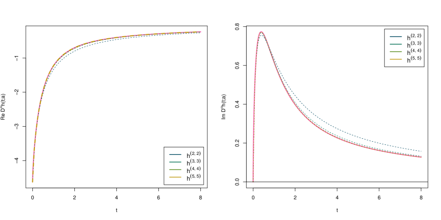
The rational approximations to for with the particular choice and rough Heston parameters (4.2) are plotted in Figure 4.1. , and are almost indistinguishable from the 1,000 step Adams estimate and significantly better than . Moreover, all of these rational approximations are at least as fast to compute as the classical Heston solution.
Naturally the coefficients of the higher order diagonal approximants become successively harder to compute in closed form. And since the formulae are more complex, the functions when implemented take longer to compute. Thus, even if, for example, were to be a better approximation than , it would be much slower to compute and would likely be the approximation of choice in practice.
4.2 Dependence of approximation quality on
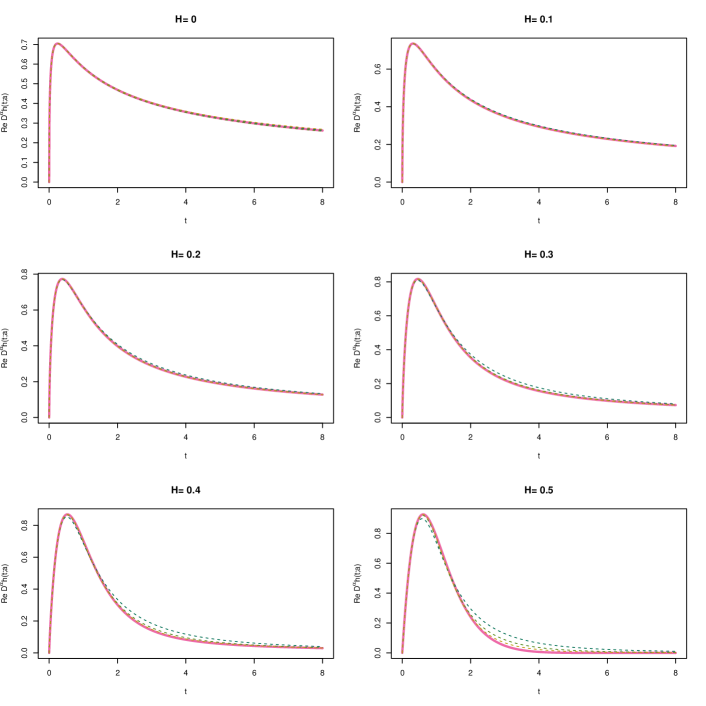
So far, we have assessed the quality of our rational approximations with the realistic but fixed set of parameters (4.2). It turns out that the quality of the rational approximations decreases as increases from to , which corresponds to the classical Heston model. Indeed, it is evident from Figure 4.2 that the approximate almost perfectly when ;111More precisely in the limit in the sense of [FGS21]. the approximation quality deteriorates as increases. Nevertheless, we observe that the approximation is very accurate, even in the classical case .
4.3 Convergence of the in the classical Heston case
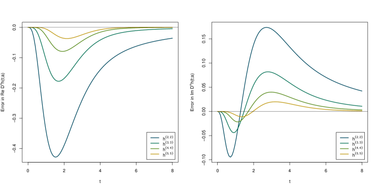
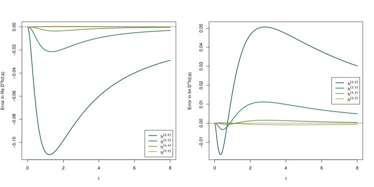
The limit of the Mittag-Leffler kernel when is the exponential, corresponding to the classical Heston model. Since we know the classical Heston characteristic function in closed form, we may study the convergence of the various rational approximations without numerical error from the Adams scheme.
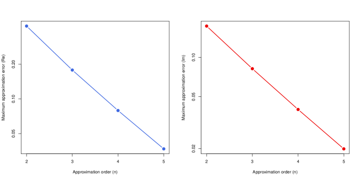
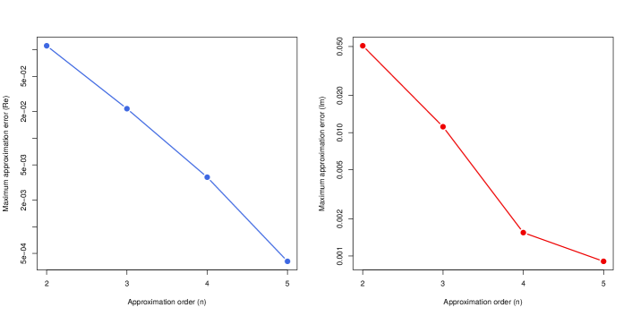
In Figure 4.3, we plot approximation errors in the classical Heston case for the Padé approximations , , , . To the naked eye, it looks as if convergence of the rational approximations may be exponential in the approximation order . This conjecture is confirmed numerically in Figure 4.4.
4.4 Convergence in the case
In the general case , there is no closed-form solution for the characteristic function, so we must measure errors relative to the Adams scheme, which is itself an approximation. We choose an intermediate value for our experiments, which is high relative to the typically estimated from time series or calibrated to implied volatilities. It is worth noting that the rational approximations are so good, that to get accurate estimates of approximation errors, the benchmark Adams scheme needs to be run with at least 1,000 steps.
In Figure 4.5, with , we plot errors for . To the naked eye, it looks as if convergence of the may once again be exponential in the approximation order . This conjecture is roughly confirmed in Figure 4.6. Note also that relative to the classical Heston case, the sizes of the errors are much smaller, consistent with Figure 4.2.
5 Summary and conclusions
The rough Heston cumulant generating function, as with all affine forward variance models, is a convolution of the forward variance curve with a function that satisfies the convolution Riccati integral equation (1.3). In [GR19] we constructed rational approximations to the solution of this equation in the special case where the kernel is power-law. In this paper, we have extended that approximation to the more general case where the kernel is a Mittag-Leffler function.
We focused on the diagonal approximants , the last three of which are efficient to compute, rendering them of great interest for practical application. Moreover, we have provided numerical evidence of exponential convergence of the with respect to the approximation order . Code is made freely available online at https://github.com/jgatheral/RationalRoughHeston.
6 Acknowledgements
We are grateful to Giacomo Bormetti and his collaborators for sharing their efficient Adams scheme code and to Stefano Marmi for enlightening conversations.
References
- [BBRR22] Fabio Baschetti, Giacomo Bormetti, Silvia Romagnoli, and Pietro Rossi. The SINC way: A fast and accurate approach to Fourier pricing. Quantitative Finance, 22(3):427–446, 2022.
- [EER19] Omar El Euch and Mathieu Rosenbaum. The characteristic function of rough Heston models. Mathematical Finance, 29(1):3–38, 2019.
- [FGS21] Martin Forde, Stefan Gerhold, and Benjamin Smith. Small-time, large-time, and asymptotics for the Rough Heston model. Mathematical Finance, 31(1):203–241, 2021.
- [Gat06] Jim Gatheral. The volatility surface: A practitioner’s guide. John Wiley & Sons, 2006.
- [GKR19] Jim Gatheral and Martin Keller-Ressel. Affine forward variance models. Finance and Stochastics, 23(3):501–533, 2019.
- [GR19] Jim Gatheral and Radoš Radoičić. Rational approximation of the rough Heston solution. International Journal of Theoretical and Applied Finance, 22(3):1950010, 2019.
- [JR16] Thibault Jaisson and Mathieu Rosenbaum. Rough fractional diffusions as scaling limits of nearly unstable heavy tailed Hawkes processes. The Annals of Applied Probability, 26(5):2860–2882, 2016.
- [Lew00] AL Lewis. Option Valuation under Stochastic Volatility. Finance Press: Newport Beach, CA, 2000.
- [Pod98] Igor Podlubny. Fractional differential equations: an introduction to fractional derivatives, fractional differential equations, to methods of their solution and some of their applications, volume 198. Elsevier, 1998.
Appendix A Asymptotic expansion of the Mittag-Leffler function
The following lemma is a straightforward corollary of Theorem 1.4 of [Pod98].
Lemma A.1.
Let and be such that
Then, for any integer , the following expansion holds:
Lemma A.2.
Let . Further let with , and let . Then for any ,
Proof.
Let . Then
which is positive, so , and so . It follows that
∎
Corollary A.1.
Let . Further let with and . Further let . For any positive integer and ,