SUPG-stabilized stabilization-free VEM: a numerical investigation

Abstract

We numerically investigate the possibility of defining stabilization-free Virtual Element (VEM) discretizations of advection-diffusion problems in the advection-dominated regime. To this end, we consider a SUPG stabilized formulation of the scheme. Numerical tests comparing the proposed method with standard VEM show that the lack of an additional arbitrary stabilization term, typical of VEM schemes, that adds artificial diffusion to the discrete solution, allows to better approximate boundary layers, in particular in the case of a low order scheme.

1 Introduction

The development of numerical methods for the solution of partial differential equations exploiting general polygonal or polyhedral meshes has been a topic of great interest in later years. Among the many families of methods developed in this context [1, 2, 3, 4, 5], this paper considers the family of Virtual Element Methods (VEM).

Since the first seminal papers [6, 7, 8, 9], VEM have been applied in many contexts where polytopal meshes can be exploited in order to better handle geometrical complexities of the computational domain, for instance we give a brief, not exhaustive, list of papers [10, 11, 12, 13, 14, 15, 16, 17, 18, 19]. Virtual element schemes are based on the definition of locally computable polynomial projections involved in the discrete bilinear forms. These forms consist of the sum of two terms: a singular one, consistent on polynomials, and a stabilizing one that ensures coercivity. In the literature, the arbitrary nature of the stabilization term remains an issue to be investigated, since it has been shown that it can cause problems in many theoretical and numerical contexts. For instance, the isotropic nature of the stabilization can become an issue in problems when devising SUPG stabilizations [20, 21].

The aim of this paper is to numerically investigate a possible solution to overcome this issue, conceiving a Virtual Element SUPG formulation that defines coercive bilinear forms without introducing an arbitrary non-polynomial stabilizing term that in the standard VEM formulation ensures the coercivity of the diffusive part of the problem. In the context of the theoretical development of a VEM scheme that do not require a stabilization term, Stabilization Free Virtual Elements Methods (SFVEM) have been recently introduced in [22], in the framework of the lowest order primal discretization of the Poisson equation. The key idea of the proposed method is to define self-stabilized bilinear forms, exploiting only higher order polynomial projections. The theoretical study of this method is an ongoing investigation, however some tests on highly anisotropic problems show that this new approach is able to overcome some issues of standard VEM related to the isotropic nature of the stabilization [23, 24].

The outline of the paper is as follows. In Section 2 we present the advection-diffusion model problem. In Section 3 we define the numerical scheme. In Section 4 we discuss the weel-posedness of the discrete problem. Section 5 is devoted to a priori error estimates. Finally, in Section 6 we present some numerical results that assess the advantages of the presented method.

In the following, $\left(\cdot,\cdot\right)_{\omega}$ denotes the $\mathrm{L}^{2}\!\left(\omega\right)$-scalar product, $\left\lVert{\cdot}\right\rVert_{\omega}$ denotes the corresponding norm, and $\left\lVert{\cdot}\right\rVert_{m,\omega}$ and $\left\lvert{\cdot}\right\rvert_{m,\omega}$ denote the $\mathrm{H}^{m}\!(\omega)$ norm and semi-norm.

2 Model Problem

Let $\Omega\subset\mathbb{R}^{2}$ be a bounded open set. We consider the following advection-diffusion model problem: find $u$ such that

$$\begin{cases}-\varepsilon\Delta u+\beta\cdot\nabla u=f&\text{in $\Omega$\,,}\\ u=0&\text{on $\partial\Omega$\,,}\end{cases}$$ (1)

where $\varepsilon>0$ is a positive real number and we make the standard hypotheses that $\beta\in\left[\mathrm{L}^{\infty}\!\left(\Omega\right)\right]^{2}$, $\nabla\cdot\beta=0$, and $f\in\mathrm{L}^{2}\!\left(\Omega\right)$. Moreover, we define the bilinear form ${B}\colon\mathrm{H}^{1}_{0}\!(\Omega)\times\mathrm{H}^{1}_{0}\!(\Omega)\to\mathbb{R}$ and the operator $F\colon\mathrm{L}^{2}\!\left(\Omega\right)\to\mathbb{R}$ such that

$${B}\left(w,v\right) =\left(\varepsilon\nabla w,\nabla v\right)_{\Omega}+\left(\beta\cdot\nabla w,v\right)_{\Omega}\quad\forall w,v\in\mathrm{H}^{1}_{0}\!(\Omega)\,,$$

$$F\left(v\right) =\left(f,v\right)_{\Omega}\quad\forall v\in\mathrm{L}^{2}\!\left(\Omega\right)\,.$$

Then, the variational formulation of (1) reads as follows: find $u\in\mathrm{H}^{1}_{0}\!(\Omega)$ such that

$${B}\left(u,v\right)=F\left(v\right)\quad\forall v\in\mathrm{H}^{1}_{0}\!(\Omega)\,.$$ (2)

It is a standard result that the above problem is well-posed under the above regularity assumptions on the data. For the sake of better readibility, we limit ourselves to homogeneous Dirichlet boundary conditions, but more general boundary conditions can be considered and will be considered in the numerical tests. Finally, for any open subset $\omega\subset\Omega$, we define:

$$\beta_{\omega}=\sup_{v\in\left[\mathrm{L}^{2}\!\left(\omega\right)\right]^{2}}\frac{\left\lVert{\beta\cdot v}\right\rVert_{\omega}}{\left\lVert{v}\right\rVert_{\omega}}\,.$$

3 Problem discretization

This section is devoted to the discretization of (2) using an enlarged enhancement Virtual Element space. The discretization defined here was introduced in its lowest order version in [22]. Here, we generalize that scheme to a generic order $k\geq 1$.

3.1 Discrete space

Let $\mathcal{M}_{h}$ denote a mesh of $\Omega$ made up of polygons. Let $h_{E}$ denote the diameter of $E\in\mathcal{M}_{h}$, and let $h=\max_{E\in\mathcal{M}_{h}}h_{E}$ be the mesh parameter. We make the following mesh assumptions, that are standard in the context of VEM [6, 9]: there exists a constant $\kappa>0$ independent of $h$ such that, for any polygon $E\in\mathcal{M}_{h}$, if ${\mathcal{E}_{h}^{E}}$ denotes the set of edges of $E$,

1. $E$ is star-shaped with respect to a ball of radius $\rho\geq\kappa h_{E}$;

2. $\forall e\in{\mathcal{E}_{h}^{E}}$, $\left\lvert{e}\right\rvert\geq\kappa h_{E}$, where $\left\lvert{e}\right\rvert$ denotes the length of $e$.

For each $E\in\mathcal{M}_{h}$, let $\mathbb{P}_{n}\!\left(E\right)$ be the space of polynomials of degree at most $n$, for any $n\in\mathbb{N}$. As a basis of $\mathbb{P}_{n}\!\left(E\right)$, we choose the following set of scaled monomials:

$$\mathcal{M}_{n}\!\left(E\right)=\left\{m_{\bm{\alpha}}\colon\mathbb{R}^{2}\to\mathbb{R}\text{ such that }m_{\bm{\alpha}}(x,y)=\frac{(x-x_{E})^{\alpha_{1}}(y-y_{E})^{\alpha_{2}}}{h_{E}}\vphantom{\frac{(x-x_{E})^{\alpha_{1}}(y-y_{E})^{\alpha_{2}}}{h_{E}}},\,\,0\leq\left\lvert{\bm{\alpha}}\right\rvert=\alpha_{1}+\alpha_{2}\leq n\right\}\,,$$

where $(x_{E},y_{E})$ is the center with respect to which $E$ is star-shaped. Moreover, let us define a subspace of $\mathcal{M}_{n}\!\left(E\right)$ given by

$$\mathcal{M}_{n,t}\!\left(E\right)=\left\{m_{\bm{\alpha}}\in\mathcal{M}_{n}\!\left(E\right)\colon\left\lvert{\bm{\alpha}}\right\rvert\geq t\right\}\quad\forall t<n\,.$$

Let $\Pi^{\nabla,E}_{n}\colon\mathrm{H}^{1}\!(E)\to\mathbb{P}_{n}\!\left(E\right)$ be the projection operator such that, $\forall v\in\mathrm{H}^{1}\!(E)$,

$$\begin{cases}\left(\nabla\Pi^{\nabla,E}_{n}v,\nabla p\right)_{E}=\left(\nabla v,\nabla p\right)_{E}&\forall p\in\mathbb{P}_{n}\!\left(E\right)\,,\\ \int_{\partial E}\Pi^{\nabla,E}_{n}v=\int_{\partial E}v&\text{if $k=1$}\,,\\ \int_{E}\Pi^{\nabla,E}_{n}v=\int_{E}v&\text{if $k>1$}\,.\end{cases}$$ (3)

Then, given $\ell_{E}\in\mathbb{N}$, $\ell_{E}\geq 0$, we introduce the enlarged enhancement VEM discrete space:

$$V_{k,\ell_{E}}^{E}=\left\{v\in\mathrm{H}^{1}\!(E)\colon\Delta v\in\mathbb{P}_{k+\ell_{E}}\!\left(E\right)\,,\gamma_{\partial E}\!\left(v\right)\in C^{0}\!\left(\partial E\right)\,,\gamma_{e}\!\left(v\right)\in\mathbb{P}_{k}\!\left(e\right)\;\forall e\in{\mathcal{E}_{h}^{E}}\,,\right.\\ \left.\left(v,p\right)_{E}=\left(\Pi^{\nabla,E}_{k}v,p\right)_{E}\;\forall p\in\mathbb{P}_{k+\ell_{E},k-2}\!\left(E\right)\right\}\,,$$ (4)

where $\gamma$ denotes the trace operator and

$$\mathbb{P}_{k+\ell_{E},k-2}\!\left(E\right)=\operatorname{\mathrm{span}}\mathcal{M}_{k+\ell_{E},k-2}\!\left(E\right)\,.$$

Remark 3.1.

The space $V_{k,0}^{E}$ is the standard VEM space used in [9, 20].

Notice that, $\forall\ell_{E}$, a possible set of degrees of freedom of $V_{k,\ell_{E}}^{E}$ corresponds to the one introduced for standard VEM spaces (see e.g. [9, 20]), that is, for any $v_{h}\in V_{k,\ell_{E}}^{E}$,

1. the values of $v$ at the vertices of $E$;

2. for each $e\in{\mathcal{E}_{h}^{E}}$, the values of $v$ at $k-1$ points internal to $e$;

3. the scaled moments $\frac{1}{\left\lvert{E}\right\rvert}\left(v,m_{\bm{\alpha}}\right)_{E}$ $\forall m_{\bm{\alpha}}\in\mathcal{M}_{k-2}\!\left(E\right)$.

3.2 Discrete problem

This section is devoted to define the SUPG-stabilized discrete version of (2). For this purpose, we adapt the scheme proposed and analysed in [20]. Notice that the discretization presented here differs from the cited one only in the bilinear form discretizing the diffusive part of the problem, while the other components of the discrete bilinear form are untouched, and so is the discrete right-hand side.

Let $E\in\mathcal{M}_{h}$ be given. If $k>1$, let $\tilde{C}_{k}$ be the largest constant, independent of $h_{E}$, such that

$$\tilde{C}_{k}h^{2}_{E}\left\lVert{\Delta p}\right\rVert_{E}^{2}\leq\left\lVert{\nabla p}\right\rVert_{E}^{2}\quad\forall p\in\mathbb{P}_{k}\!\left(E\right)\,.$$ (5)

Such an inequality is a standard inverse inequalities for polynomials (see e.g. [25]). In particular, $\tilde{C}_{k}$ depends on the constant $\kappa$ in the mesh assumptions, and on the degree $k$. Notice that it does not depend on $\ell_{E}$. The Péclet number associated to $E$ is defined as

$$\mathrm{Pe}_{E}=m_{k}\frac{\beta_{E}h_{E}}{\varepsilon}\,,\quad m_{k}=\begin{cases}\frac{1}{3}&\text{if $k=1$,}\\ 2\tilde{C}_{k}&\text{if $k>1$.}\end{cases}$$

Following the standard Streamline Upwind Petrov-Galerkin approach [26], for any $E\in\mathcal{M}_{h}$ let the parameter $\tau_{E}$ be given, such that

$$\tau_{E}=\frac{h_{E}}{2\beta_{E}}\min\left\{1,\mathrm{Pe}_{E}\right\}\,,$$ (6)

and we define the symmetric positive definite tensor $\varepsilon_{\beta,E}=\varepsilon+\tau_{E}\beta\beta^{\intercal}$. Notice that, by the hypotheses on $\beta$, this tensor satisfies, $\forall E\in\mathcal{M}_{h}$, $\forall\bm{v}\in\left[\mathrm{L}^{2}\!\left(E\right)\right]^{2}$,

$$\sqrt{\varepsilon}\left\lVert{\bm{v}}\right\rVert_{E}\leq\left\lVert{\sqrt{\varepsilon_{\beta,E}}\bm{v}}\right\rVert_{E}\leq\sqrt{\left(\varepsilon+\tau_{E}\beta_{E}^{2}\right)}\left\lVert{\bm{v}}\right\rVert_{E}\,.$$

To define the SUPG formulation of the problem, we introduce the space

$$\mathrm{H}^{1,\Delta}_{\mathrm{loc}}\!(\mathcal{M}_{h})=\left\{v\in\mathrm{H}^{1}_{0}\!(\Omega)\colon\Delta v\in\mathrm{L}^{2}\!\left(E\right)\quad\forall E\in\mathcal{M}_{h}\right\}\,,$$

and, $\forall E\in\mathcal{M}_{h}$, the bilinear form ${\mathcal{B}}^{E}\colon\mathrm{H}^{1,\Delta}_{\mathrm{loc}}\!(\mathcal{M}_{h})\times\mathrm{H}^{1}_{0}\!(\Omega)\to\mathbb{R}$ such that, $\forall w\in\mathrm{H}^{1,\Delta}_{\mathrm{loc}}\!(\mathcal{M}_{h})$, $\forall v\in\mathrm{H}^{1}_{0}\!(\Omega)$,

$${\mathcal{B}}^{E}\left(w,v\right)={a}^{E}\left(w,v\right)+{b}^{E}\left(w,v\right)+{d}^{E}\left(w,v\right)\,,$$

where

$${a}^{E}\left(w,v\right) =\left(\varepsilon\nabla w,\nabla v\right)_{E}+\tau_{E}\left(\beta\cdot\nabla w,\beta\cdot\nabla v\right)_{E}\,,$$

$${b}^{E}\left(w,v\right) =\left(\beta\cdot\nabla w,v\right)_{E}\,,$$

$${d}^{E}\left(w,v\right) =-\tau_{E}\left(\varepsilon\Delta w,\beta\cdot\nabla v\right)_{E}\,.$$

Moreover, we introduce the operator $\mathcal{F}^{E}\colon\mathrm{H}^{1}\!(E)\to\mathbb{R}$ such that

$$\mathcal{F}^{E}\left(v\right)=\left(f,v+\tau_{E}\beta\cdot\nabla v\right)_{E}\quad\forall v\in\mathrm{H}^{1}\!(E)\,.$$

The above operators are not computable from the degrees of freedom for functions in $V_{k,\ell_{E}}^{E}$. For this reason, we define discrete bilinear forms involving polynomial projections of VEM discrete functions. In the spirit of [22], for a given $n\in\mathbb{N}$ let $\Pi^{0,E}_{n}\colon\left[\mathrm{L}^{2}\!\left(E\right)\right]^{2}\to\left[\mathbb{P}_{n}\!\left(E\right)\right]^{2}$ denote the $\left[\mathrm{L}^{2}\!\left(E\right)\right]^{2}$ projection onto $\left[\mathbb{P}_{n}\!\left(E\right)\right]^{2}$ and let

$${a}^{E}_{h}\left(w,v\right) =\left(\varepsilon\Pi^{0,E}_{k+\ell_{E}-1}\nabla w,\Pi^{0,E}_{k+\ell_{E}-1}\nabla v\right)_{E}+\tau_{E}\left(\beta\cdot\Pi^{0,E}_{k+\ell_{E}-1}\nabla w,\beta\cdot\Pi^{0,E}_{k+\ell_{E}-1}\nabla v\right)_{E}\,,$$

$${b}^{E}_{h}\left(w,v\right) =\left(\beta\cdot\Pi^{0,E}_{k-1}\nabla w,\Pi^{0,E}_{k-1}v\right)_{E}\,,$$

$${d}^{E}_{h}\left(w,v\right) =-\tau_{E}\left(\varepsilon\nabla\cdot\left(\Pi^{0,E}_{k-1}\nabla w\right),\beta\cdot\Pi^{0,E}_{k+\ell_{E}-1}\nabla v\right)_{E}\,.$$

Remark 3.2.

Notice that, contrarily to standard VEM SUPG formulations (cf. [20, 21]), here we do not require an additional arbitrary stabilization term in the bilinear form ${a}^{E}_{h}$. The choice of the parameter $\ell_{E}$ is done in order to guarantee coercivity of ${a}^{E}_{h}$, as detailed in the next section.

Finally, to state our discrete problem, we define the bilinear form ${\mathcal{B}}^{E}_{h}\colon\mathrm{H}^{1,\Delta}_{\mathrm{loc}}\!(\mathcal{M}_{h})\times\mathrm{H}^{1}_{0}\!(\Omega)\to\mathbb{R}$ such that, $\forall w\in\mathrm{H}^{1,\Delta}_{\mathrm{loc}}\!(\mathcal{M}_{h})$, $\forall v\in\mathrm{H}^{1}_{0}\!(\Omega)$,

$${\mathcal{B}}^{E}_{h}\left(w,v\right)={a}^{E}_{h}\left(w,v\right)+{b}^{E}_{h}\left(w,v\right)+{d}^{E}_{h}\left(w,v\right)\,,$$

and the operator $\mathcal{F}_{h}^{E}\colon\mathrm{H}^{1}\!(E)\to\mathbb{R}$ such that

$$\mathcal{F}_{h}^{E}\left(v\right)=\left(f,\Pi^{0,E}_{k-1}v+\tau_{E}\beta\cdot\Pi^{0,E}_{k+\ell_{E}-1}\nabla v\right)_{E}\quad\forall v\in\mathrm{H}^{1}\!(E)\,.$$

Then, let

$$V_{k,\ell}=\left\{v\in\mathrm{H}^{1}_{0}\!(\Omega)\colon v\in V_{k,\ell_{E}}^{E}\;\forall E\in\mathcal{M}_{h}\right\}\,,$$

our discretization of (2) requires to find $u_{h}\in V_{k,\ell}$ such that

$$\sum_{E\in\mathcal{M}_{h}}{\mathcal{B}}^{E}_{h}\left(u_{h},v_{h}\right)=\sum_{E\in\mathcal{M}_{h}}\mathcal{F}_{h}^{E}\left(v_{h}\right)\quad\forall v_{h}\in V_{k,\ell}\,.$$ (7)

4 Well-posedness

The aim of this section is to discuss the key points needed for the well-posedness of (7). It is currently an open problem to prove theoretically a robust criterium to choose $\ell_{E}$ for any kind of polygon, in such a way that ${a}^{E}_{h}$ is coercive. Thus, we assume that there exists at least a good choice of $\ell_{E}$ for each type of polygon and in Section 6 we perform a numerical investigation of it.

Assumption 4.1.

We assume that, $\forall k\geq 1$ $\exists\ell_{E}$ such that $\exists\alpha>0$ independent of $h_{E}$ satisfying

$$\left\lVert{\Pi^{0,E}_{k+\ell_{E}-1}\nabla v_{h}}\right\rVert_{E}^{2}\geq\alpha\left\lVert{\nabla v_{h}}\right\rVert_{E}^{2}\quad\forall v_{h}\in V_{k,\ell_{E}}^{E}\,.$$ (8)

From now on, we set $\ell_{E}$ as the smallest integer satisfying Assumption 4.1. With this choice, we define the following VEM-SUPG norm:

$$\left\lvert\left\lvert\left\lvert v_{h}\right\rvert\right\rvert\right\rvert^{2}=\sum_{E\in\mathcal{M}_{h}}\limits{a}^{E}_{h}\left(v_{h},v_{h}\right)\quad\forall v_{h}\in V_{k,\ell}\,.$$

Then, we can prove the following well-posedness result.

Theorem 4.1.

Under Assumption 4.1, we have, $\forall E\in\mathcal{M}_{h}$ and for $h$ sufficiently small,

$$\exists C>0\colon\sum_{E\in\mathcal{M}_{h}}\limits{\mathcal{B}}^{E}_{h}\left(v_{h},v_{h}\right)\geq C\left\lvert\left\lvert\left\lvert v_{h}\right\rvert\right\rvert\right\rvert^{2}\quad\forall v_{h}\in V_{k,\ell_{E}}^{E}\,.$$

Proof.

Let $v_{h}\in V_{k,\ell_{E}}^{E}$ be given. First, exploiting the definition of $\tau_{E}$ in (6), the inverse inequality (5) and Young inequalities, we get,

$$\left\lvert{{d}^{E}_{h}\left(v_{h},v_{h}\right)}\right\rvert=\tau_{E}\left\lvert{\left(\varepsilon\nabla\cdot\left(\Pi^{0,E}_{k-1}\nabla v_{h}\right),\beta\cdot\Pi^{0,E}_{k+\ell_{E}-1}\nabla v_{h}\right)_{E}}\right\rvert\\ \leq\frac{m_{k}h^{2}_{E}}{4\varepsilon}\left\lVert{\varepsilon\nabla\cdot\left(\Pi^{0,E}_{k-1}\nabla v_{h}\right)}\right\rVert_{E}^{2}+\frac{\tau_{E}}{2}\left\lVert{\beta\cdot\Pi^{0,E}_{k+\ell_{E}-1}\nabla v_{h}}\right\rVert_{E}^{2}\leq\frac{1}{2\varepsilon}\left\lVert{\varepsilon\Pi^{0,E}_{k-1}\nabla v_{h}}\right\rVert_{E}^{2}+\frac{\tau_{E}}{2}\left\lVert{\beta\cdot\Pi^{0,E}_{k+\ell_{E}-1}\nabla v_{h}}\right\rVert_{E}^{2}\\ \leq\frac{\varepsilon}{2}\left\lVert{\Pi^{0,E}_{k-1}\nabla v_{h}}\right\rVert_{E}^{2}+\frac{\tau_{E}}{2}\left\lVert{\beta\cdot\Pi^{0,E}_{k+\ell_{E}-1}\nabla v_{h}}\right\rVert_{E}^{2}\\ \leq\frac{\varepsilon}{2}\left\lVert{\Pi^{0,E}_{k+\ell_{E}-1}\nabla v_{h}}\right\rVert_{E}^{2}+\frac{\tau_{E}}{2}\left\lVert{\beta\cdot\Pi^{0,E}_{k+\ell_{E}-1}\nabla v_{h}}\right\rVert_{E}^{2}=\frac{1}{2}{a}^{E}_{h}\left(v_{h},v_{h}\right)\,.$$

Thus, it follows

$${a}^{E}_{h}\left(v_{h},v_{h}\right)+{d}^{E}_{h}\left(v_{h},v_{h}\right)\geq\frac{1}{2}{a}^{E}_{h}\left(v_{h},v_{h}\right)=\frac{1}{2}\left\lvert\left\lvert\left\lvert v_{h}\right\rvert\right\rvert\right\rvert_{E}^{2}\,.$$ (9)

Moreover, since ${b}\left(v_{h},v_{h}\right)=0$, we get

$$\left\lvert{\sum_{E\in\mathcal{M}_{h}}{b}^{E}_{h}\left(v_{h},v_{h}\right)}\right\rvert=\left\lvert{\sum_{E\in\mathcal{M}_{h}}\left(\beta\cdot\Pi^{0,E}_{k-1}\nabla v_{h},\Pi^{0,E}_{k-1}v_{h}\right)_{E}}\right\rvert=\left\lvert{\sum_{E\in\mathcal{M}_{h}}\left(\Pi^{0,E}_{k-1}\left(\beta\cdot\Pi^{0,E}_{k-1}\nabla v_{h}\right),v_{h}\right)_{E}}\right\rvert\\ =\left\lvert{\sum_{E\in\mathcal{M}_{h}}\left(\Pi^{0,E}_{k-1}\left(\beta\cdot\Pi^{0,E}_{k-1}\nabla v_{h}\right)-\beta\cdot\nabla v_{h},v_{h}\right)_{E}}\right\rvert=\left\lvert{\sum_{E\in\mathcal{M}_{h}}\left(\beta\cdot\Pi^{0,E}_{k-1}\nabla v_{h}-\beta\cdot\nabla v_{h},\Pi^{0,E}_{k-1}v_{h}-v_{h}\right)_{E}}\right\rvert\\ \leq\sum_{E\in\mathcal{M}_{h}}\left\lVert{\beta\cdot\left(\Pi^{0,E}_{k-1}\nabla v_{h}-\nabla v_{h}\right)}\right\rVert_{E}\left\lVert{\Pi^{0,E}_{k-1}v_{h}-v_{h}}\right\rVert_{E}\leq C_{\varepsilon\beta}\sum_{E\in\mathcal{M}_{h}}h_{E}\left\lvert\left\lvert\left\lvert v_{h}\right\rvert\right\rvert\right\rvert_{E}^{2}\,,$$

where $C_{\varepsilon\beta}$ depends in particular on the problem data and the equivalence constant in (8). Collecting the latest estimate and (9), we get the thesis:

$$\sum_{E\in\mathcal{M}_{h}}\limits{\mathcal{B}}^{E}_{h}\left(v_{h},v_{h}\right)\geq\left(\frac{1}{2}-C_{\varepsilon\beta}h\right)\left\lvert\left\lvert\left\lvert v_{h}\right\rvert\right\rvert\right\rvert^{2}\,.$$

∎

Notice that the above result is analogous to the one obtained in [20] in the case of standard VEM. Notice that other choices are possible to discretize the transport term (see [27]), and they would lead to a similar well-posedness result.

5 Error analysis

In this section we address the a priori error analysis of the presented scheme, under Assumption 4.1. The analysis follows the techniques already used to prove a priori estimates for standard VEM schemes [9, 20, 27]. We provide some details about the interpolation properties of the considered space, since it is a slight modification of the classical VEM spaces, due to the enlarged enhancement property.

In the following we prove an interpolation estimate onto the space $V_{k,\ell_{E}}^{E}$ defined by (4). The proof follows the one in [28] for the interpolation on standard VEM spaces. First of all we prove an auxiliary result, introducing an inverse inequality in $V_{k,\ell_{E}}^{E}$.

Lemma 5.1.

Let $E\in\mathcal{M}_{h}$ and let $w\in\mathrm{H}^{1}\!(E)$ such that $\Delta w\in\mathbb{P}_{k+\ell}\!\left(E\right)$, for some chosen $\ell\geq 0$. Then, there exists a constant $C_{I}$ such that

$$\left\lVert{\Delta w}\right\rVert_{E}\leq C_{I}h_{E}^{-1}\left\lVert{\nabla w}\right\rVert_{E}\,.$$ (10)

The constant $C_{I}$ depends on $k$, $\ell_{E}$ and on the mesh regularity parameter $\kappa$.

Proof.

First, let $p\in\mathbb{P}_{k+\ell}\!\left(E\right)$. Then, let $\psi_{E}\in\mathrm{H}^{1}_{0}\!(E)$ be a bubble function defined on a regular sub-triangulation of $E$ (see [28]), such that $1\geq\psi_{E}\geq 0$. Then, since $\psi_{E}p\in\mathrm{H}^{1}_{0}\!(E)$,

$$\left\lVert{p}\right\rVert_{\mathrm{H}^{-1}\!(E)}=\sup_{v\in\mathrm{H}^{1}_{0}\!(E)}\frac{\left(p,v\right)_{E}}{\left\lVert{\nabla v}\right\rVert_{E}}\geq\frac{\left(\psi_{E},p^{2}\right)_{E}}{\left\lVert{\nabla(\psi_{E}p)}\right\rVert_{E}}\geq C_{B}\frac{\left\lVert{p}\right\rVert_{E}^{2}}{h_{E}^{-1}\left\lVert{p}\right\rVert_{E}}=C_{B}h_{E}\left\lVert{p}\right\rVert_{E}\,,$$

where we use the fact that, since $\psi_{E}$ is non-negative and bounded, $\sqrt{\left(\psi_{E},p^{2}\right)_{E}}$ is a norm on $\mathbb{P}_{k+\ell}\!\left(E\right)$, and thus equivalent to $\left\lVert{p}\right\rVert_{E}$. Similarly, since $\psi_{E}\in\mathrm{H}^{1}_{0}\!(E)$, $\left\lVert{\nabla(\psi_{E}p)}\right\rVert_{E}$ is a norm on $\mathbb{P}_{k+\ell}\!\left(E\right)$, and standard scaling arguments provide the weight $h_{E}^{-1}$. It follows that $C_{B}$ depends on $k$, $\ell$ and on the shape regularity of $E$.

Taking $p=\Delta w$ in the above result and applying Green’s theorem and a Cauchy-Schwarz inequality, we conclude, defining $C_{I}=C_{B}^{-1}$,

$$\left\lVert{\Delta w}\right\rVert_{E}\leq C_{I}h_{E}^{-1}\sup_{v\in\mathrm{H}^{1}_{0}\!(E)}\frac{\left(\Delta w,v\right)_{E}}{\left\lVert{\nabla v}\right\rVert_{E}}=C_{I}h_{E}^{-1}\sup_{v\in\mathrm{H}^{1}_{0}\!(E)}\frac{\left(-\nabla w,\nabla v\right)_{E}}{\left\lVert{\nabla v}\right\rVert_{E}}\leq C_{I}h_{E}^{-1}\left\lVert{\nabla w}\right\rVert_{E}\,.$$

∎

Theorem 5.1.

Let $u\in\mathrm{H}^{s}\!(\Omega)$, $1\leq s\leq k+1$. Let $\ell_{E}\in\mathbb{N}$ be given $\forall E\in\mathcal{M}_{h}$. There $\exists u_{I}\in V_{k,\ell}$ such that

$$\exists C>0\colon\left\lVert{u-u_{I}}\right\rVert_{\Omega}+h\left\lVert{\nabla(u-u_{I})}\right\rVert_{\Omega}\leq Ch^{s}\left\lvert{u}\right\rvert_{s,\Omega}\,.$$ (11)

Proof.

Following [28], let $\mathcal{T}_{h}$ be the sub-triangulation of $\mathcal{M}_{h}$ obtained as the union of local sub-triangulations of each polygon $E\in\mathcal{M}_{h}$, linking each vertex to the center of the ball with respect to which $E$ is star-shaped. Naturally, $\mathcal{T}_{h}$ inherits the shape-regularity of $\mathcal{M}_{h}$. Let $u_{C}\in\mathbb{P}_{k}\!\left(\mathcal{T}_{h}\right)$ be the piecewise polynomial over $\mathcal{T}_{h}$ defined as the Clément interpolant of $u$ over $\mathcal{T}_{h}$. This is obtained by local projections of $u$ onto piecewise polynomials defined on patches of triangles that share a degree of freedom, see [29]. It holds (see [29, Theorem 1])

$$\left\lvert{u-u_{C}}\right\rvert_{m,\Omega}\leq C_{Cl,k}h^{s-m}\left\lvert{u}\right\rvert_{s}\,m\leq s\,,$$ (12)

where $C_{Cl,k}$ depends on the shape-regularity of $\mathcal{M}_{h}$ and the order $k$. Let $w_{I}\in\mathrm{H}^{1}\!(\Omega)$ be the function that solves, $\forall E\in\mathcal{M}_{h}$,

$$\begin{cases}-\Delta w_{I}=-\Delta\Pi^{0,E}_{k}u_{C}&\text{in $E$}\,,\\ w_{I}=u_{C}&\text{on $\partial E$}\,.\end{cases}$$ (13)

By the definition of $w_{I}$ we have that, $\forall E\in\mathcal{M}_{h}$, $\Pi^{0,E}_{k}\left(u_{C}\right)-w_{I}$ solves the following problem:

$$\begin{cases}-\Delta(\Pi^{0,E}_{k}u_{C}-w_{I})=0&\text{in $E$}\,,\\ \Pi^{0,E}_{k}u_{C}-w_{I}=\Pi^{0,E}_{k}u_{C}-u_{C}&\text{on $\partial E$}\,.\end{cases}$$

It follows that

$$\left\lVert{\nabla(\Pi^{0,E}_{k}u_{C}-w_{I})}\right\rVert_{E}=\inf\{\left\lVert{\nabla z}\right\rVert_{E}\,,z\in\mathrm{H}^{1}\!(E)\colon\gamma_{\partial E}\!\left(z\right)=\Pi^{0,E}_{k}u_{C}-u_{C}\}\leq\left\lVert{\nabla(\Pi^{0,E}_{k}u_{C}-u_{C})}\right\rVert_{E}\,,$$

which implies, exploiting the continuity of the operator $\Pi^{0,E}_{k}$ and (12),

$$\left\lVert{\nabla(u_{C}-w_{I})}\right\rVert_{E}\leq\left\lVert{\nabla(u_{C}-\Pi^{0,E}_{k}u_{C})}\right\rVert_{E}+\left\lVert{\nabla(\Pi^{0,E}_{k}u_{C}-w_{I})}\right\rVert_{E}\\ \leq 2\left\lVert{\nabla\left(\Pi^{0,E}_{k}u_{C}-u_{C}\right)}\right\rVert_{E}\leq 2C_{\Pi,k}\left\lVert{\nabla u_{C}}\right\rVert_{E}\leq 2C_{\Pi,k}C_{Cl,k}\left\lVert{\nabla u}\right\rVert_{E}\,,$$ (14)

where $C_{\Pi,k}$ depends on the shape-regularity of $E$ and the order $k$. We define $u_{I}\in V_{k,\ell}$ such that $\forall E\in\mathcal{M}_{h}$

$$\gamma_{e}\!\left(u_{I}\right) =\gamma_{e}\!\left(w_{I}\right)\quad\forall e\in\partial E\,,$$ (15)

$$\left(u_{I}-w_{I},p\right)_{E} =0\quad\forall p\in\mathbb{P}_{k-2}\!\left(E\right)\,,$$ (16)

$$\left(u_{I}-\Pi^{\nabla,E}_{k}w_{I},p\right)_{E} =0\quad\forall p\in\mathbb{P}_{k+\ell_{E},k-2}\!\left(E\right)\,.$$ (17)

Notice that applying Green’s theorem we get from (15) and (16) that $\Pi^{\nabla,E}_{k}u_{I}=\Pi^{\nabla,E}_{k}w_{I}$ nd thus (17) implies

$$\left(u_{I}-\Pi^{\nabla,E}_{k}u_{I},p\right)_{E}=0\quad\forall p\in\mathbb{P}_{k+\ell_{E},k-2}\!\left(E\right)\,.$$ (18)

We now prove (11) for $u_{I}$. Concerning $\mathrm{H}^{1}\!(\Omega)$-seminorm of $u-u_{I}$, recalling (12) we get

$$\begin{split}\left\lVert{\nabla(u-u_{I})}\right\rVert_{\Omega}&\leq\left\lVert{\nabla(u-u_{C})}\right\rVert_{\Omega}+\left\lVert{\nabla(u_{C}-u_{I})}\right\rVert_{\Omega}\\ &\leq C_{Cl,k}h^{s-1}\left\lvert{u}\right\rvert_{s,\Omega}+\left(\sum_{E\in\mathcal{M}_{h}}\left\lVert{\nabla(u_{C}-u_{I})}\right\rVert_{E}^{2}\right)^{\frac{1}{2}}\,.\end{split}$$

Moreover, from the definition of $w_{I}$ (13) and the definition of $u_{I}$ (15) we get $\gamma_{e}\!\left(u_{C}\right)=\gamma_{e}\!\left(w_{I}\right)=\gamma_{e}\!\left(u_{I}\right)$ for each edge $e$ of $\mathcal{M}_{h}$. Thus, $u_{C}-u_{I}\in\mathrm{H}^{1}_{0}\!(E)$ $\forall E\in\mathcal{M}_{h}$. We can thus estimate the $\mathrm{L}^{2}\!\left(\Omega\right)$-norm of $u-u_{I}$ as follows:

$$\begin{split}\left\lVert{u-u_{I}}\right\rVert_{\Omega}&\leq\left\lVert{u-u_{C}}\right\rVert_{\Omega}+\left\lVert{u_{C}-u_{I}}\right\rVert_{\Omega}\\ &\leq C_{Cl,k}h^{s}\left\lvert{u}\right\rvert_{s,\Omega}+\left(\sum_{E\in\mathcal{M}_{h}}\left\lVert{u_{C}-u_{I}}\right\rVert_{E}^{2}\right)^{\frac{1}{2}}\\ &\leq C_{Cl,k}h^{s}\left\lvert{u}\right\rvert_{s,\Omega}+h\left(\sum_{E\in\mathcal{M}_{h}}C_{p,E}\left\lVert{\nabla(u_{C}-u_{I})}\right\rVert_{E}^{2}\right)^{\frac{1}{2}}\,,\end{split}$$ (19)

where $C_{p,E}$ depends on the shape-regularity of $E$. We now focus on estimating $\left\lVert{\nabla(u_{C}-u_{I})}\right\rVert_{E}$ $\forall E\in\mathcal{M}_{h}$. Applying (14) we get

$$\begin{split}\left\lVert{\nabla(u_{C}-u_{I})}\right\rVert_{E}&\leq\left\lVert{\nabla(u_{C}-w_{I})}\right\rVert_{E}+\left\lVert{\nabla(w_{I}-u_{I})}\right\rVert_{E}\\ &\leq 2C_{\Pi,k}C_{Cl,k}\left\lVert{\nabla u}\right\rVert_{E}+\left\lVert{\nabla(w_{I}-u_{I})}\right\rVert_{E}\,.\end{split}$$ (20)

Finally, the last term can be bounded applying Green’s theorem (recall that $w_{I}-u_{I}\in\mathrm{H}^{1}_{0}\!(E)$), (16), (18), the fact that $\Pi^{\nabla,E}_{k}u_{I}=\Pi^{\nabla,E}_{k}w_{I}$, a Cauchy-Schwarz inequality, the approximation properties of polynomial projections, (14) and the inverse inequality (10) we get

$$\begin{split}\left\lVert{\nabla(w_{I}-u_{I})}\right\rVert_{E}^{2}&=-\left(\Delta(w_{I}-u_{I}),w_{I}-u_{I}\right)_{E}\\ &=-\left(\Delta(w_{I}-u_{I})-\Pi^{0,E}_{k-2}\left(\Delta(w_{I}-u_{I})\right),w_{I}-u_{I}\right)_{E}\\ &=-\left(\Delta(w_{I}-u_{I})-\Pi^{0,E}_{k-2}\left(\Delta(w_{I}-u_{I})\right),w_{I}-\Pi^{\nabla,E}_{k}u_{I}\right)_{E}\\ &=-\left(\Delta(w_{I}-u_{I})-\Pi^{0,E}_{k-2}\left(\Delta(w_{I}-u_{I})\right),w_{I}-\Pi^{\nabla,E}_{k}w_{I}\right)_{E}\\ &\leq\left\lVert{\Delta(w_{I}-u_{I})-\Pi^{0,E}_{k-2}\left(\Delta(w_{I}-u_{I})\right)}\right\rVert_{E}\left\lVert{w_{I}-\Pi^{\nabla,E}_{k}w_{I}}\right\rVert_{E}\\ &\leq C\left\lVert{\Delta(w_{I}-u_{I})}\right\rVert_{E}\cdot h_{E}\left\lVert{\nabla w_{I}}\right\rVert_{E}\\ &\leq C\left\lVert{\Delta(w_{I}-u_{I})}\right\rVert_{E}\cdot h_{E}\left\lVert{\nabla u}\right\rVert_{E}\\ &\leq C\left\lVert{\nabla(w_{I}-u_{I})}\right\rVert_{E}\left\lVert{\nabla u}\right\rVert_{E}\,.\end{split}$$

Then, collecting (19), (20) and the last estimate, we obtain (11). ∎

The interpolation estimate provided by Theorem 5.1 along with approximation results analogous to the ones obtained in [20, 27] are used to prove the following a priori error estimates, whose proof is omitted since it is analogous to the one in the cited references.

Theorem 5.2.

Assume $u\in\mathrm{H}^{s+1}\!(\Omega)$ and $f\in\mathrm{H}^{s-1}\!(\Omega)$. Then, under the current regularity assumptions and if $\ell_{E}$ is chosen $\forall E\in\mathcal{M}_{h}$ in such a way that (8) holds,

$$\left\lvert\left\lvert\left\lvert u-u_{h}\right\rvert\right\rvert\right\rvert\leq Ch^{s}\left(\max_{E\in\mathcal{T}_{h}}\{1,\sqrt{h_{E}\beta_{E}}\}\left\lVert{u}\right\rVert_{s+1}+C_{f,\varepsilon\beta}\left\lVert{f}\right\rVert_{s-1}\right)\,,$$

where $C$ is independent of $h$ and on the problem coefficients and $C_{f,\varepsilon\beta}$ depends on local variations of the problem coefficients.

6 Numerical Results

In this section we present two numerical experiments, namely Test 1 in Section 6.1 and Test 2 in Section 6.2. In the first test we confirm the convergence rates predicted by the a priori error analysis of Section 5 and we compare our method with the standard SUPG virtual element discretization [20] in terms of relative energy errors. In the second test we consider a classic problem taken from [26] involving approximation of internal and boundary layers. In all the numerical tests our aim is to assess the robustness of the approach in case of advection dominated regime. Therefore, all the benchmark problems are characterized by high mesh Péclet numbers. Moreover, for each type of polygon in each mesh considered in the tests, we have done a preliminary assessment of the minimum $\ell_{E}$ that satisfies Assumption 4.1. This is done computing the two smallest eigenvalues of the local stiffness matrix $A^{E}$, defined as $A^{E}_{ij}=\left(\Pi^{0,E}_{k+\ell_{E}-1}\nabla\phi_{i},\Pi^{0,E}_{k+\ell_{E}-1}\nabla\phi_{j}\right)_{E}$, where $\{\phi_{i}\}$ denotes the set of local basis functions of the VEM space on a polygon $E\in\mathcal{M}_{h}$. We consider SFVEM of different orders from one to three and a unit square domain $\Omega=(0,1)\times(0,1)$.

6.1 Test 1

In this first test, we consider an advection-diffusion problem characterized by a diffusivity parameter $\varepsilon=10^{-9}$ and a transport velocity field $\beta=(1,0.545)$. The size of the meshes is chosen to guarantee that for the selected value of $\varepsilon$ the mesh Péclet number is much greater than one for all $k$. The forcing term $f$ and the boundary conditions are such that the exact solution (depicted in Figure 1) is

$$u(x,y)=c_{1}\ xy\ (x-1)(y-1)\ e^{-c_{2}(c_{4}(c_{2}-x)^{2}+c_{3}(c_{2}-y)^{2}-c_{3}(c_{2}-x)(c_{2}-y))},$$

where $c_{1}=\frac{3}{\sqrt{2\pi}}$, $c_{2}=\frac{1}{2}$, $c_{3}=1000$ and $c_{4}=\frac{1}{3.3}\cdot 10^{3}$. The selected solution $u$ is characterized by a strong anisotropy. Indeed, in Figure 1, we can see that the solution exhibits a strong boundary layer in a direction approximately perpendicular to the direction of the transport velocity field $\beta$.

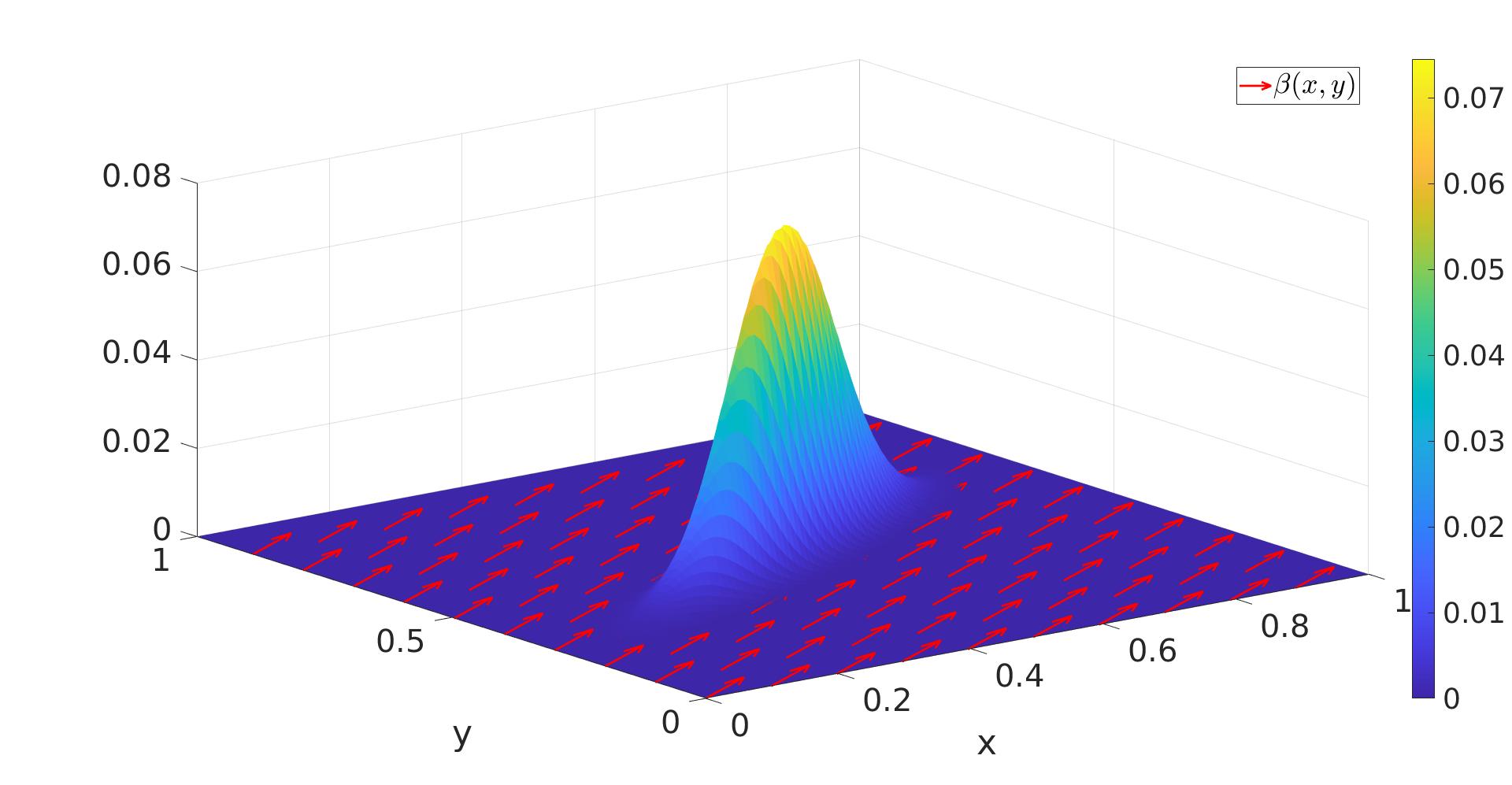
Figure 1: Test 1: exact solution $u(x,y)$ and transport velocity field $\beta(x,y)$ (red arrows).

To study the convergence of the method, we consider three different families of meshes ($\mathcal{T}_{1}$, $\mathcal{T}_{2}$ and $\mathcal{T}_{3}$) and four different refinements for each one of them. The first mesh of each sequence is reported in Figure 2.

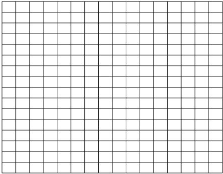
(a)

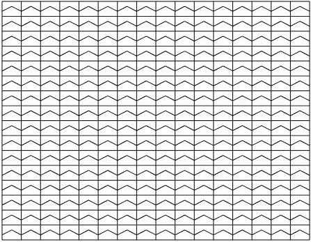
(b)

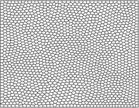
(c)

Figure 2: Meshes.

[b] $\mathcal{T}_{1}$ $\mathcal{T}_{2}$ $\mathcal{T}_{3}$ $k$ 1 2 3-4 1 2 3-4 1 2 3-4 $\mathcal{M}_{first}$ $2\cdot 10^{7}$ $4\cdot 10^{6}$ $1\cdot 10^{6}$ $1\cdot 10^{7}$ $3\cdot 10^{6}$ $8\cdot 10^{5}$ $6\cdot 10^{6}$ $2\cdot 10^{6}$ $4\cdot 10^{5}$ $\mathcal{M}_{last}$ $2\cdot 10^{6}$ $5\cdot 10^{5}$ $1\cdot 10^{5}$ $2\cdot 10^{6}$ $4\cdot 10^{5}$ $1\cdot 10^{5}$ $2\cdot 10^{6}$ $5\cdot 10^{5}$ $1\cdot 10^{5}$

Table 1: Test 1: Mean values of the mesh Péclet number for the first mesh $\mathcal{M}_{first}$ and last mesh $\mathcal{M}_{last}$ of the mesh families $\mathcal{T}_{1}$, $\mathcal{T}_{2}$ and $\mathcal{T}_{3}$.

The mesh family $\mathcal{T}_{1}$ consists of standard cartesian elements, the mesh family $\mathcal{T}_{2}$ is composed of both concave and convex polygons and the mesh family $\mathcal{T}_{3}$ has been constructed using Polymesher [30]. The first two groups of meshes are refined splitting the existing elements in half. For the last group of meshes this approach is not feasible. Therefore, we simply increase the number of elements by means of Polymesher. Consequently, the tessellations of this family include polygons having different numbers of edges. Moreover, in Table 1 we report also the mean mesh Péclet number for the first mesh and the last mesh of each mesh family.

[b] $\mathcal{T}_{1}$ $\mathcal{T}_{2}$ $\mathcal{T}_{3}$ $N^{V}_{E}$ 4 5 1-4 5 6 7 $k=1$ 1 1 1 1 2 2 $k=2$ 2 1 1 1 2 2 $k=3$ 2 1 1 1 2 2 $k=4$ 2 2 1 2 3 4

Table 2: Values of $\ell_{E}$ for the proposed method and tessellations $\mathcal{T}_{1}$, $\mathcal{T}_{2}$ and $\mathcal{T}_{3}$, related to the number of vertices $N_{E}^{V}$ of the polygons in each mesh.

Now, for each type of polygon of the meshes analyzed, we have to discuss the proper choice of $\ell_{E}$. This choice has been done, as said previously, selecting the value $\ell_{E}$ that guarantees the numerical coercivity of the local stiffness matrix. In Table 2, we report the values of $\ell_{E}$ computed following this criterion and adopted specifically to solve the problem described in the present subsection. Notice that $\ell_{E}$ does not depend only on the number of vertices of the polygon, but also on its geometry. Indeed, if we consider the line corresponding to $k=2$ in Table 2, we can see that we require $\ell_{E}=2$ for $\mathcal{T}_{1}$, where quadrilaterals are all squares, and $\ell_{E}=1$ for $\mathcal{T}_{3}$, that features generally shaped quadrilaterals.

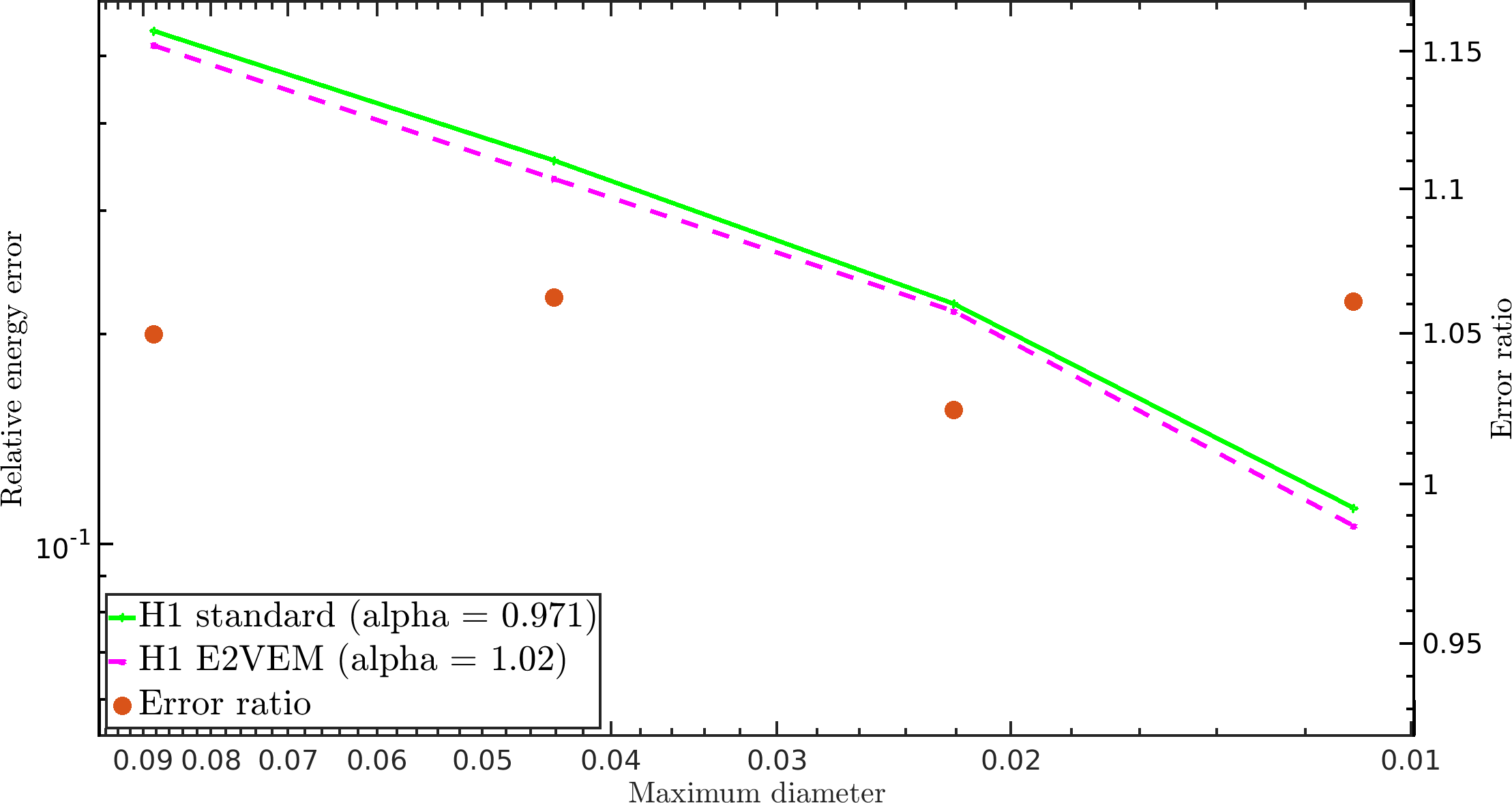
(a)

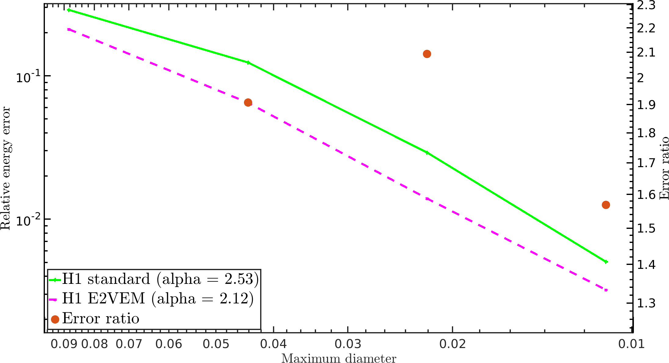
(b)

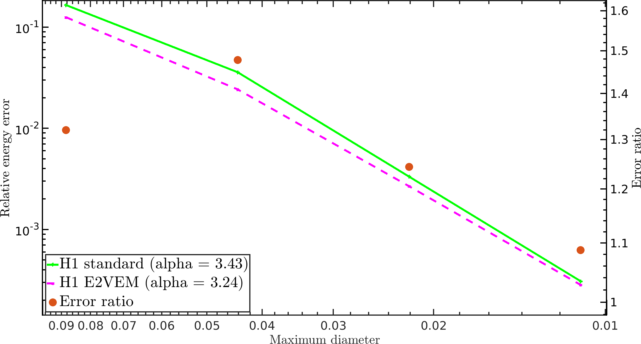
(c)

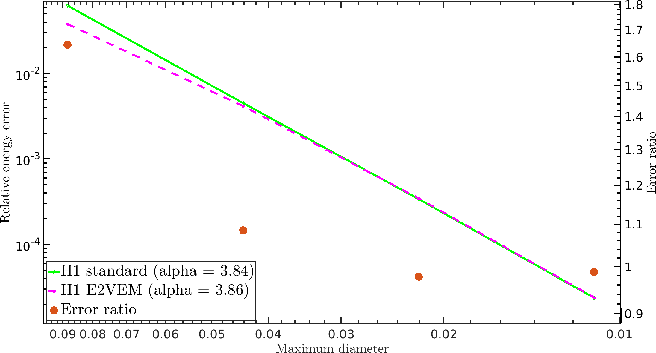
(d)

Figure 3: Test 1: convergence curves (tessellation $\mathcal{T}_{1}$).

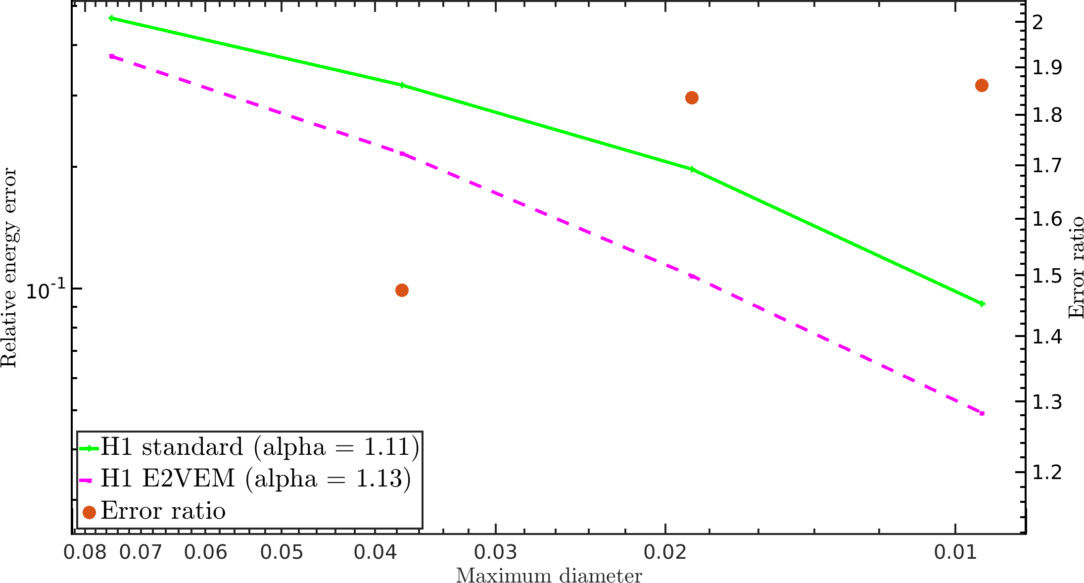
(a)

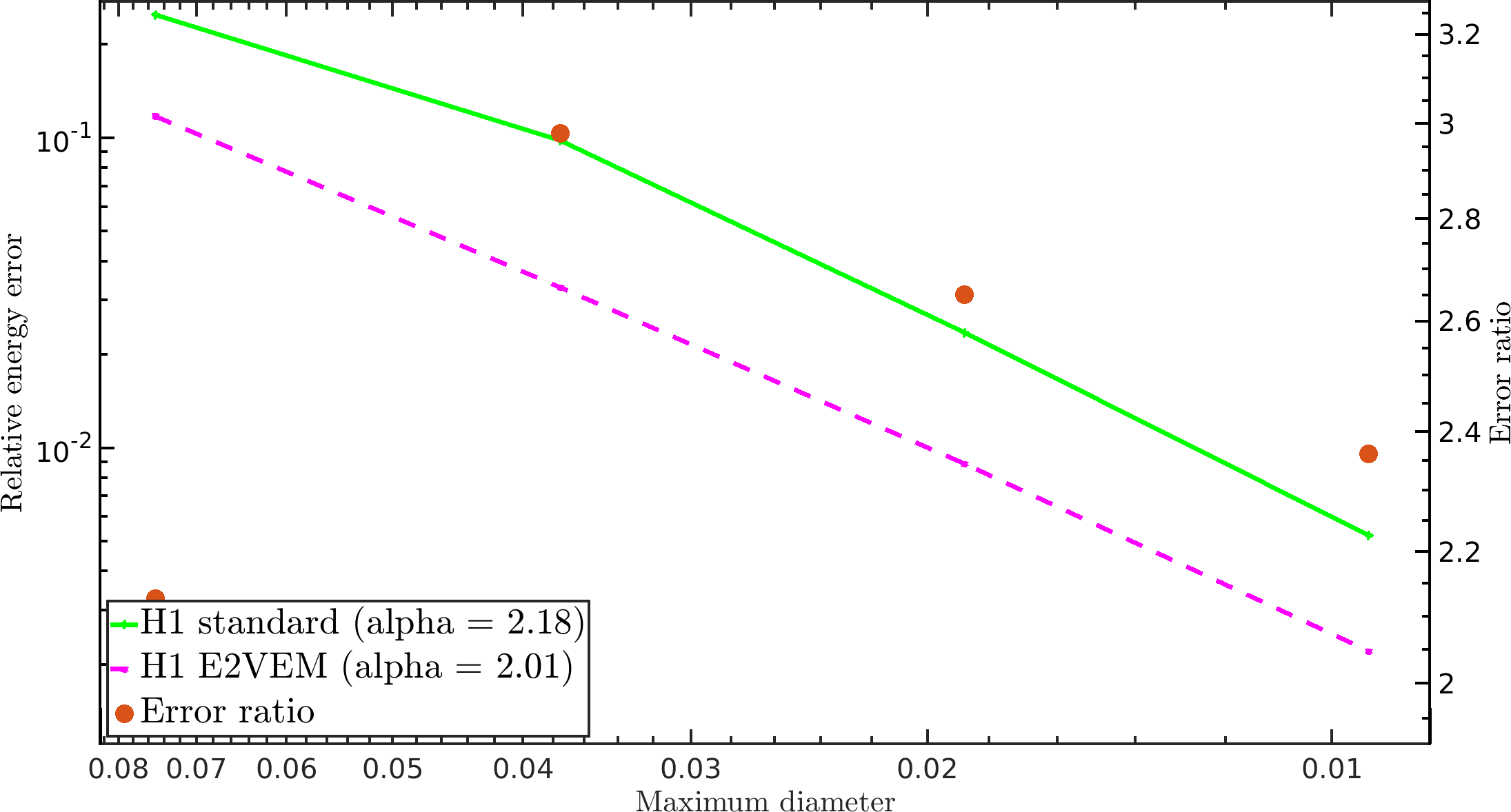
(b)

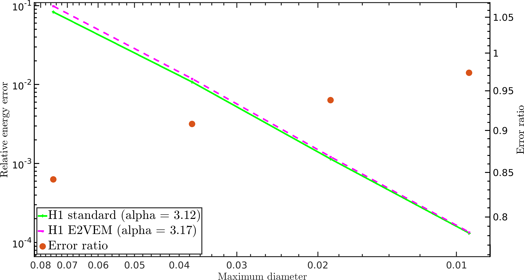
(c)

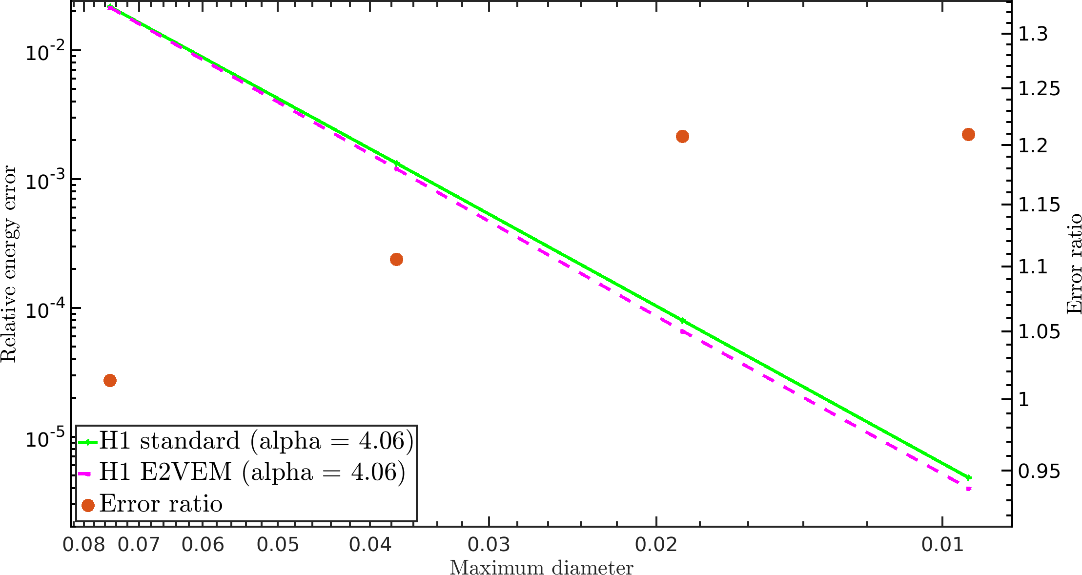
(d)

Figure 4: Test 1: convergence curves (tessellation $\mathcal{T}_{2}$).

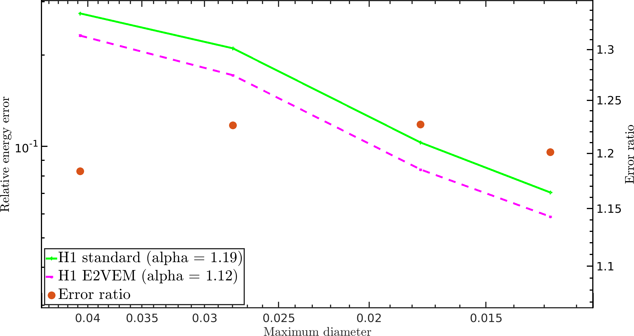
(a)

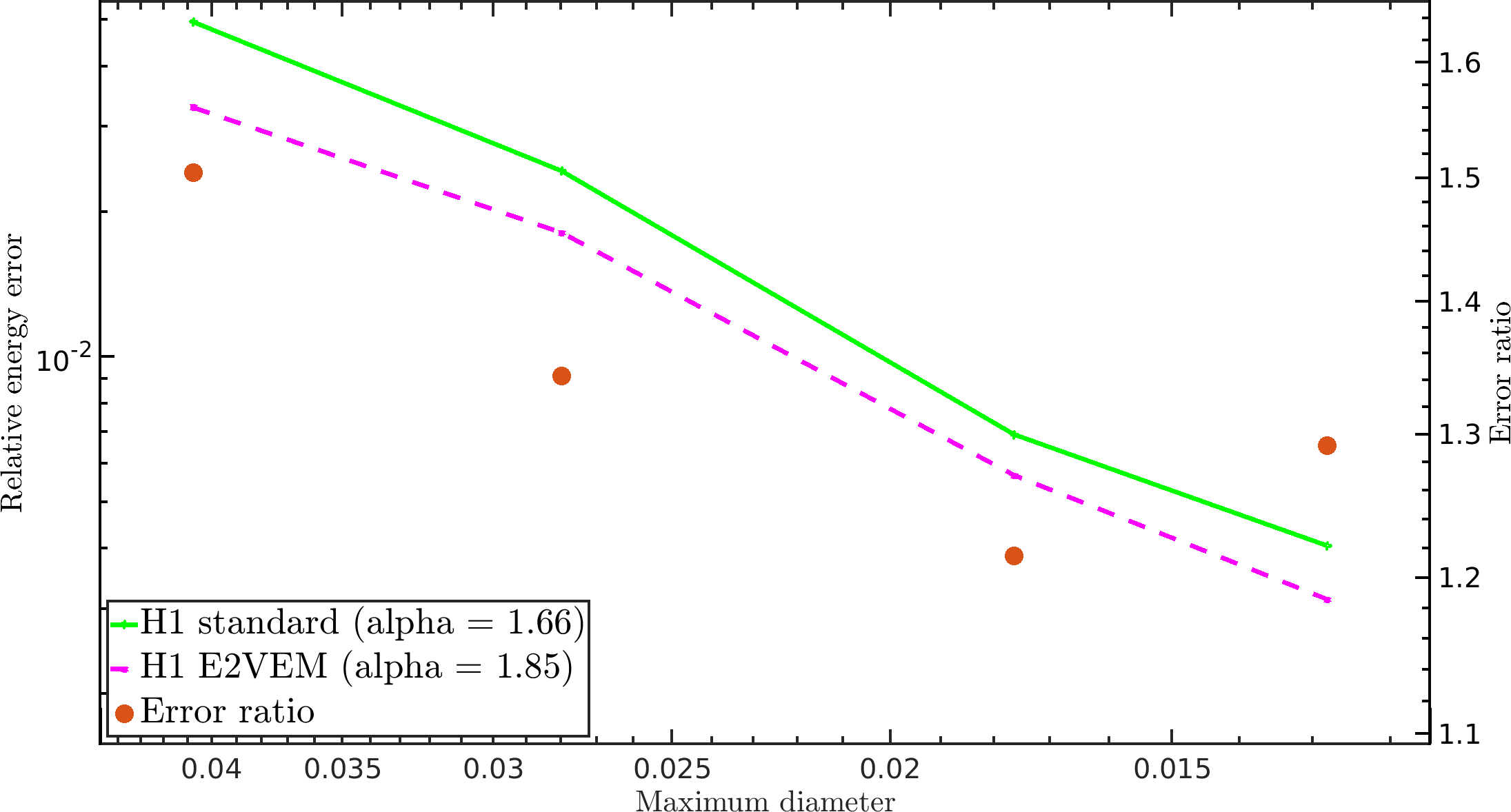
(b)

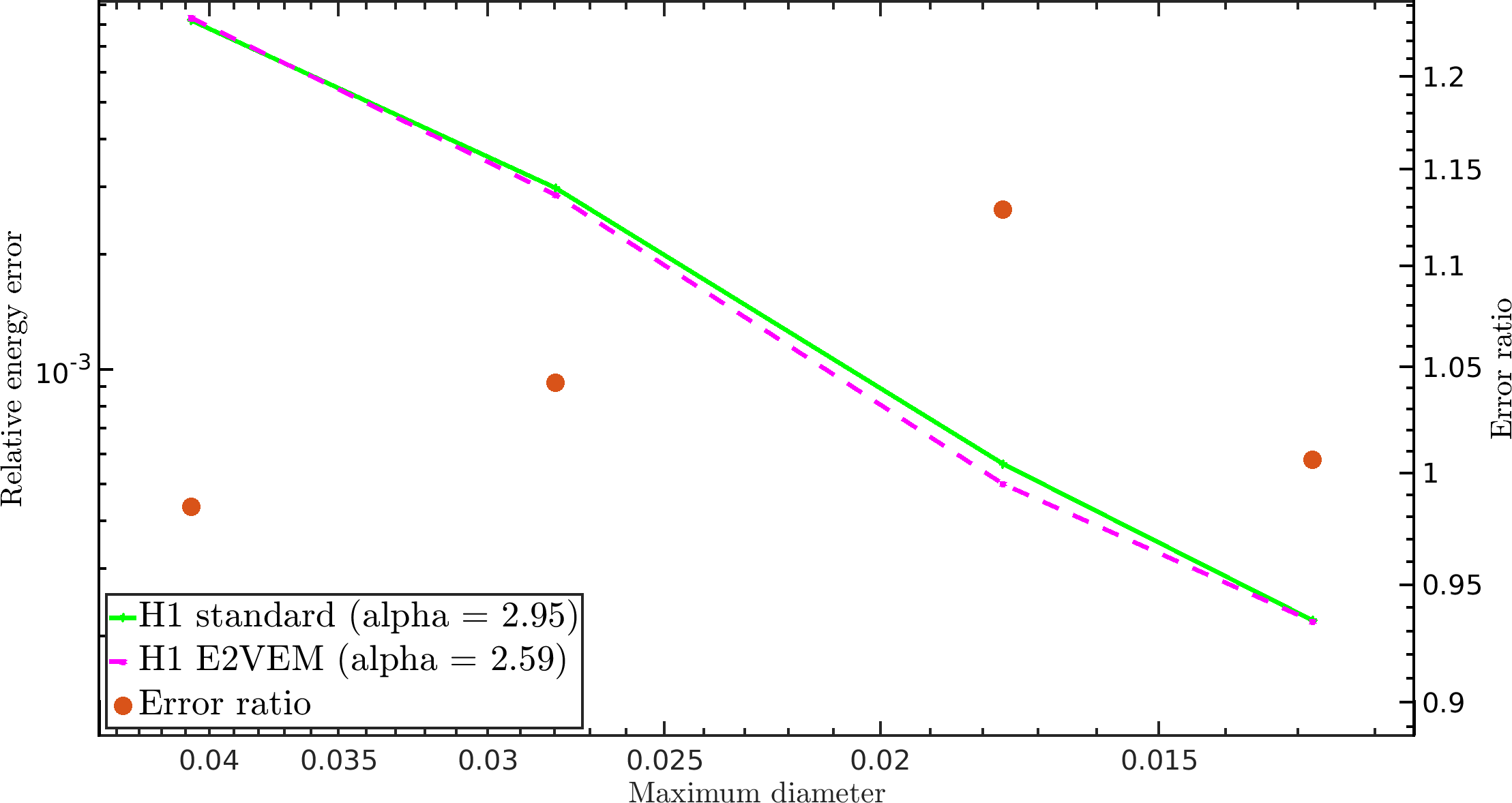
(c)

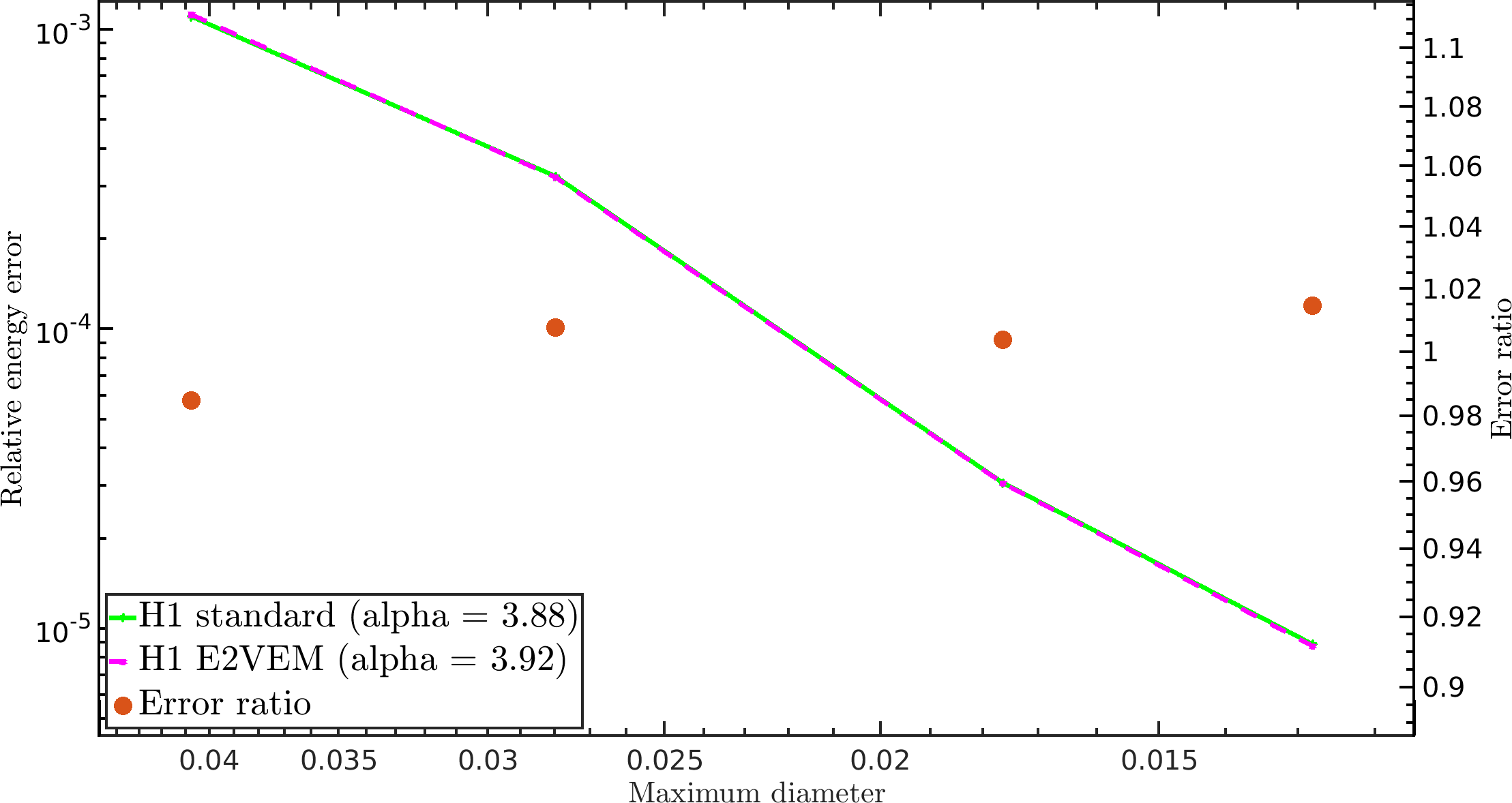
(d)

Figure 5: Test 1: convergence curves (tessellation $\mathcal{T}_{3}$).

In Figures 3, 4 and 5 we show the convergence curves in log-log scale. We report the relative errors computed in the energy norm plotted against the maximum diameter of the discretization for both the SFVEM and the classical VEM [20] and for orders from $1$ to $4$. The computed relative error is based on the difference between the exact solution and the projection $\Pi^{\nabla,E}_{k}$ of the discrete solution $u_{h}$ and it is given by the following expression

$$err=\displaystyle\sqrt{\frac{\sum_{E\in\mathcal{M}_{h}}\left\lVert{\sqrt{\varepsilon}\nabla(u-\Pi^{\nabla,E}_{k}u_{h})}\right\rVert_{E}^{2}+\tau_{E}\left\lVert{\beta\cdot\nabla(u-\Pi^{\nabla,E}_{k}u_{h})}\right\rVert_{E}^{2}}{\sum_{E\in\mathcal{M}_{h}}\left\lVert{\sqrt{\varepsilon}\nabla u}\right\rVert_{E}^{2}+\tau_{E}\left\lVert{\beta\cdot\nabla u}\right\rVert_{E}^{2}}}\,.$$

The charts of Figures  3, 4 and 5 display two y-axis: the one on the left is related to the relative energy error, whereas the one on the right is related to the ratio between the VEM error and the SFVEM error. In the legend, alpha denotes the numerical rates of convergence, computed using the last two meshes of each refinement. The numerical rates of convergence for both the two methods are in agreement with the theoretical findings for the energy norm of the problem (Theorem 5.2).

Figures 3a, 5a and 4a show that for order $k=1$ the two methods provide very close results on the mesh family $\mathcal{T}_{1}$, whereas the SFVEM over performs the classical VEM on the mesh families $\mathcal{T}_{2}$ and $\mathcal{T}_{3}$. Thus, the results suggest that the SFVEM is able to decrease the magnitude of the error with respect to the classical VEM when dealing with solutions characterized by strong anisotropies. Indeed, the possibility to avoid an arbitrary stabilizing part enhances the performance of the method. An analogous trend is observed for $k=2$, though in this case we observe better performances also for the cartesian mesh $\mathcal{T}_{1}$. Moreover, in Figures 4a and 4b we notice that the error difference between the SFVEM and the VEM seems to be even stronger than the one observed in Figures 3a, 3b, 5a and 5b. We believe that this could be related to the presence of non-convex elements.

Figures 3c, 3d, 4c, 4d, 5c and 5d show that for $k=3$ and $k=4$ the VEM and the SFVEM exhibit an almost equivalent behaviour for all the considered meshes. A similar trend was also observed for anisotropic elliptic problems in [23]. Indeed, for higher orders we expect that the polynomial part of the VEM bilinear form tends to predominate the stabilizing part reducing the error gap between the two methods.

6.2 Test 2

For the second test, we consider a classic benchmark problem in the SUPG literature characterized by the presence of different layers. This problem was originally proposed in the context of standard Finite Element Methods in [26].

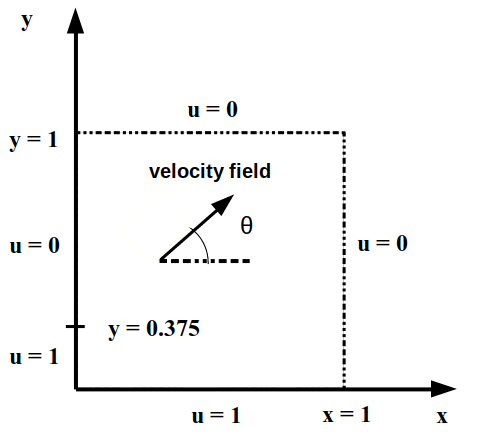
Figure 6: Test 2: computational domain and boundary conditions.

The computational domain $\Omega$ as well as the boundary conditions are illustrated in Figure 6. Notice the discontinuous Dirichlet boundary condition on the left side of the domain. The diffusion coefficient is set equal to $\varepsilon=10^{-6}$, the velocity field is $\beta=(\cos{\theta},\sin{\theta})$, where $\theta=\frac{\pi}{4}$, and the forcing term $f$ is null. The resulting Péclet number is very large (around $10^{6}$). At the inflow boundary, the velocity propagates the non-homogeneous boundary condition originating an internal boundary layer, whereas at the outflow boundary an outflow boundary layer is produced due to the homogeneous boundary conditions.

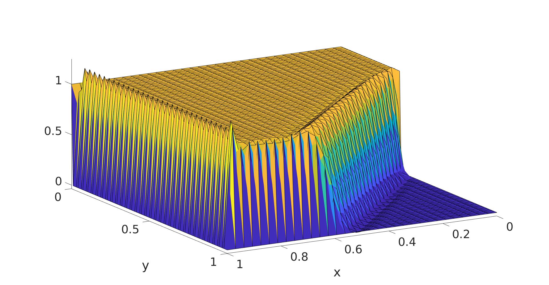
(a)

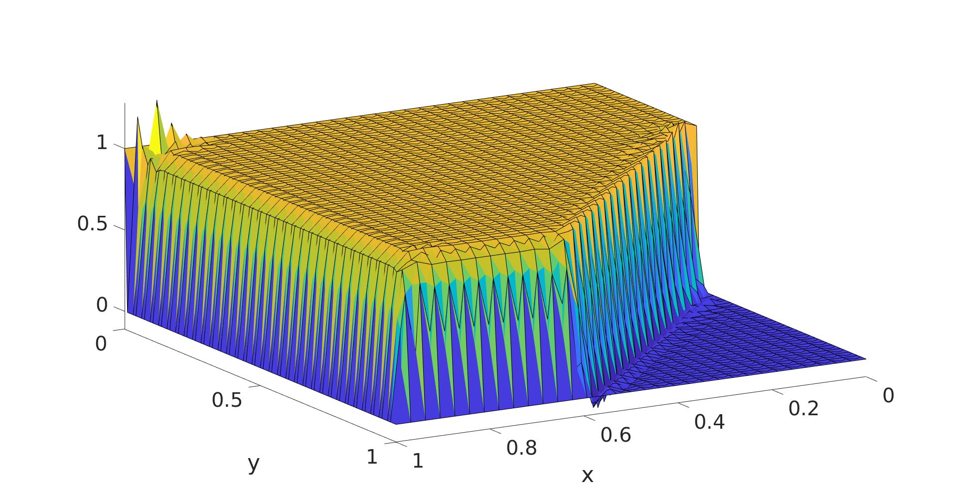
(b)

Figure 7: Test 2: SFVEM solution for $k=1$ and $k=3$ on $\mathcal{T}_{2}$.

We solve the problem using $\mathcal{T}_{2}$ tessellation, depicted in Figure 2b. Figures 7a and 7b show the results obtained for SFVEM of order $k=1$ and $k=3$. The numerical solutions are comparable to the ones presented in [26, 20, 21]. As it is typical for this problem we notice the presence of undershoots and overshoots near the internal boundary layer. Moreover, smoother solutions are obtained increasing the order of the method.

7 Conclusions

We presented a numerical investigation of the performances of SUPG-stabilized stabilization-free VEM, assessing the possibility of using higher-order polynomial projectors in the definition of the discrete bilinear form and avoiding the use of a stabilizing bilinear form. We also provided an interpolation estimate for the new scheme, analogous to the one obtained for standard VEM. Numerical results show that the possibility of avoiding a stabilizing bilinear form, that adds some artificial diffusion to the problem in order to ensure coercivity, can enhance the performances of classical VEM methods when there is the need to approximate strong boundary layers, as in the case of convection dominated problems.

References

• [1] D.. Di Pietro and A. Ern “Hybrid high-order methods for variable-diffusion problems on general meshes” In Comptes Rendus Mathematique 353.1, 2015, pp. 31–34 DOI: 10.1016/j.crma.2014.10.013
• [2] M. Cicuttin, A. Ern and N. Pignet “Hybrid High-Order Methods. A primer with application to solid mechanics” In Hybrid High-Order Methods. A primer with application to solid mechanics Springer Cham, 2021 DOI: 10.1007/978-3-030-81477-9
• [3] F. Brezzi, K. Lipnikov and V. Simoncini “A family of mimetic finite difference methods on polygonal and polyhedral meshes” In Mathematical Models and Methods in Applied Sciences 15.10, 2005, pp. 1533–1551 DOI: 10.1142/S0218202505000832
• [4] B. Rivière “Discontinuous Galerkin Methods for Solving Elliptic and Parabolic Equations” Society for IndustrialApplied Mathematics, 2008 DOI: 10.1137/1.9780898717440
• [5] N. Sukumar and A. Tabarraei “Conforming polygonal finite elements” In International Journal for Numerical Methods in Engineering 61.12, 2004, pp. 2045–2066 DOI: 10.1002/nme.1141
• [6] L. Beirão da Veiga, F. Brezzi, A. Cangiani, G. Manzini, L.. Marini and A. Russo “Basic principles of virtual element methods” In Mathematical Models and Methods in Applied Sciences 23.01, 2013, pp. 199–214 DOI: 10.1142/S0218202512500492
• [7] L. Veiga, F. Brezzi and L.. Marini “Virtual Elements for linear elasticity problems” In SIAM journal on numerical analysis 51.2 Philadelphia: Society for IndustrialApplied Mathematics, 2013, pp. 794–812
• [8] L. Beirão da Veiga, F. Brezzi, L.. Marini and A. Russo “The Hitchhiker’s Guide to the Virtual Element Method” In Mathematical Models and Methods in Applied Sciences 24.8 World Scientific Publishing Company, 2014, pp. 1541–1573 DOI: 10.1142/S021820251440003X
• [9] L. Beirão da Veiga, F. Brezzi, L.. Marini and A. Russo “Virtual Element Methods for General Second Order Elliptic Problems on Polygonal Meshes” In Mathematical Models and Methods in Applied Sciences 26.04, 2015, pp. 729–750 DOI: 10.1142/S0218202516500160
• [10] L. Beirão da Veiga, C. Lovadina and D. Mora “A Virtual Element Method for elastic and inelastic problems on polytope meshes” In Computer Methods in Applied Mechanics and Engineering 295, 2015, pp. 327–346 DOI: 10.1016/j.cma.2015.07.013
• [11] E. Artioli, S. Miranda, C. Lovadina and L. Patruno “A stress/displacement Virtual Element method for plane elasticity problems” In Computer Methods in Applied Mechanics and Engineering 325, 2017, pp. 155–174 DOI: https://doi.org/10.1016/j.cma.2017.06.036
• [12] F. Dassi, C. Lovadina and M. Visinoni “A three-dimensional Hellinger–Reissner virtual element method for linear elasticity problems” In Computer Methods in Applied Mechanics and Engineering 364, 2020, pp. 112910 DOI: https://doi.org/10.1016/j.cma.2020.112910
• [13] F. Dassi, C. Lovadina and M. Visinoni “Hybridization of the virtual element method for linear elasticity problems” In Mathematical Models and Methods in Applied Sciences 31.14, 2021, pp. 2979–3008 DOI: 10.1142/S0218202521500676
• [14] M.. Benedetto, S. Berrone and A. Borio “The Virtual Element Method for underground flow simulations in fractured media” In Advances in Discretization Methods 12, SEMA SIMAI Springer Series Switzerland: Springer International Publishing, 2016, pp. 167–186 DOI: 10.1007/978-3-319-41246-7˙8
• [15] M.. Benedetto, S. Berrone, A. Borio, S. Pieraccini and S. Scialò “A Hybrid Mortar Virtual Element Method For Discrete Fracture Network Simulations” In Journal of Computational Physics 306, 2016, pp. 148–166 DOI: 10.1016/j.jcp.2015.11.034
• [16] M.. Benedetto, A. Borio and A. Scialò “Mixed Virtual Elements for discrete fracture network simulations” In Finite Elements in Analysis and Design 134, 2017, pp. 55–67 DOI: https://doi.org/10.1016/j.finel.2017.05.011
• [17] S. Berrone, M. Busetto and F. Vicini “Virtual Element simulation of two-phase flow of immiscible fluids in Discrete Fracture Networks” In Journal of Computational Physics 473, 2023, pp. 111735 DOI: https://doi.org/10.1016/j.jcp.2022.111735
• [18] A. Borio, F.. Hamon, N. Castelletto, J.. White and R.. Settgast “Hybrid mimetic finite-difference and virtual element formulation for coupled poromechanics” In Computer Methods in Applied Mechanics and Engineering 383, 2021, pp. 113917 DOI: https://doi.org/10.1016/j.cma.2021.113917
• [19] S. Berrone and M. Busetto “A virtual element method for the two-phase flow of immiscible fluids in porous media” In Computational Geosciences 26, 2022, pp. 195–216 DOI: https://doi.org/10.1007/s10596-021-10116-4
• [20] M.. Benedetto, S. Berrone, A. Borio, S. Pieraccini and S. Scialò “Order preserving SUPG stabilization for the virtual element formulation of advection-diffusion problems” In Comput. Methods Appl. Mech. Engrg. 311, 2016, pp. 18–40 DOI: 10.1016/j.cma.2016.07.043
• [21] S. Berrone, A. Borio and G. Manzini “SUPG stabilization for the nonconforming virtual element method for advection–diffusion–reaction equations” In Computer Methods in Applied Mechanics and Engineering 340, 2018, pp. 500–529 DOI: 10.1016/j.cma.2018.05.027
• [22] S. Berrone, A. Borio and F. Marcon “Lowest order stabilization free Virtual Element Method for the Poisson equation”, arXiv:2103.16896 [math.NA], 2021 arXiv:2103.16896 [math.NA]
• [23] S. Berrone, A. Borio and F. Marcon “Comparison of standard and stabilization free Virtual Elements on anisotropic elliptic problems” In Applied Mathematics Letters 129, 2022, pp. 107971 DOI: 10.1016/j.aml.2022.107971
• [24] S. Berrone, A. Borio, F. Marcon and G. Teora “A first-order stabilization-free Virtual Element Method” In Applied Mathematics Letters 142, 2023, pp. 108641 DOI: https://doi.org/10.1016/j.aml.2023.108641
• [25] S.. Brenner and L.. Scott “The Mathematical Theory of Finite Element Methods”, Texts in Applied Mathematics Springer New York, NY, 2008 DOI: 10.1007/978-0-387-75934-0
• [26] L.. Franca, S.. Frey and T… Hughes “Stabilized finite element methods: I. Application to the advective-diffusive model” In Computer Methods in Applied Mechanics and Engineering 95.2 Elsevier, 1992, pp. 253–276
• [27] L. Beirão da Veiga, F. Dassi, C. Lovadina and G. Vacca “SUPG-stabilized virtual elements for diffusion-convection problems: a robustness analysis” In ESAIM: M2AN 55.5, 2021, pp. 2233–2258 DOI: 10.1051/m2an/2021050
• [28] A. Cangiani, E.. Georgoulis, T. Pryer and O.. Sutton “A posteriori error estimates for the virtual element method” In Numerische Mathematik 137.4, 2017, pp. 857–893 DOI: 10.1007/s00211-017-0891-9
• [29] P. Clément “Approximation by finite element functions using local regularization” In Revue française d’automatique, informatique, recherche opérationnelle. Analyse numérique 9.R2 EDP Sciences, 1975, pp. 77–84
• [30] C. Talischi, G.. Paulino, A. Pereira and I… Menezes “PolyMesher: A general-purpose mesh generator for polygonal elements written in Matlab” In Struct. Multidiscipl. Optim. 45.3, 2012, pp. 309–328 DOI: 10.1007/s00158-011-0706-z