Measurement of the small-scale 3D Lyman-$\alpha$ forest power spectrum

Abstract

Small-scale correlations measured in the Lyman-$\alpha$ (Ly$\alpha$) forest encode information about the intergalactic medium and the primordial matter power spectrum. In this article, we present and implement a simple method to measure the 3-dimensional power spectrum, $P_{\rm{3}D}$, of the Ly$\alpha$ forest at wavenumbers $k$ corresponding to small, $\sim$ Mpc scales. In order to estimate $P_{\rm{3}D}$ from sparsely and unevenly distributed data samples, we rely on averaging 1-dimensional Fourier Transforms, as previously carried out to estimate the 1-dimensional power spectrum of the Ly$\alpha$ forest, $P_{\rm{1}D}$. This methodology exhibits a very low computational cost. We confirm the validity of this approach through its application to Nyx cosmological hydrodynamical simulations. Subsequently, we apply our method to the eBOSS DR16 Ly$\alpha$ forest sample, providing as a proof of principle, a first $P_{\rm{3}D}$ measurement averaged over two redshift bins $z=2.2$ and $z=2.4$. This work highlights the potential for forthcoming $P_{\rm{3}D}$ measurements, from upcoming large spectroscopic surveys, to untangle degeneracies in the cosmological interpretation of $P_{\rm{1}D}$.

1 Introduction

The Ly$\alpha$ forest is a well-established observational tool in cosmology. When light from a distant object travels through a medium containing neutral hydrogen HI, it can undergo resonant absorption at a specific wavelength $\lambda_{\alpha}=1215.67$ Å. The HI component of the inhomogeneously-distributed intergalactic medium (IGM), located between a distant source and a terrestrial observer, therefore imprints its observed optical spectrum with the so-called Ly$\alpha$ forest [1, 2]. Consequently, the spatial distribution of Ly$\alpha$ forest data is composed of sparse and irregularly distributed lines-of-sight throughout the IGM. This geometry complicates the determination of the Ly$\alpha$ forest 3-dimensional power spectrum, $P_{\rm{3}D}$. In this article, we implement a method to measure $P_{\rm{3}D}$ which addresses this issue by resorting to Fourier transforms, exclusively in one dimension along these lines-of-sight.

As a cosmological observable, the Ly$\alpha$ forest is currently the best probe of large scale structures, at least on a statistical ground, for $2<z\lesssim 4$. Within this specific redshift range, it is expected that the impacts of non-linearities and galaxy feedback on the matter distribution are less pronounced compared to $z\lesssim 1.5$, which is the main target of current galaxy surveys [3]. Furthermore, hydrodynamical simulations have demonstrated that, except for the case of high-column density absorbers, the Ly$\alpha$ forest is produced mostly by the dilute part of the IGM, associated with under-dense or mildly over-dense regions of the cosmic web [4, 5]. This makes the Ly$\alpha$ forest sensitive to the matter power spectrum $P(k)$ at small scales $k\sim$ Mpc, in a way directly connected to the primordial linear matter power spectrum at these scales [6, 7].

To study the small-scale matter distribution from Ly$\alpha$ forest observations, an efficient approach consists of measuring 1-dimensional correlations between absorption intensities within individual optical spectra of background sources. The statistical estimator of choice is the Fourier transform of the corresponding correlation function, the 1-dimensional power spectrum $P_{\rm{1}D}$$(k_{\parallel})$, where $k_{\parallel}$ is the wavenumber associated with the absorber’s coordinate along a line-of-sight (LOS). Following the initial work by [6, 8], numerous $P_{\rm{1}D}$ measurements have been carried out over the past two decades, spanning a wide range of scales and redshifts. Some of these measurements have focused on large $k_{\parallel}$, with relatively small samples of high-resolution, high signal-to-noise spectra, e.g. [7, 9, 10, 11, 12, 13, 14]. In contrast, some measurements were conducted down to smaller $k_{\parallel}\sim 0.1$ Mpc^-1, e.g. [15, 16, 17, 18, 19], relying on the large statistics achieved by cosmological spectroscopic surveys. Cosmological simulations including thermal properties of the IGM allow one to model the Ly$\alpha$ absorption field [20, 21, 22]. Since, as explained above, the measured Ly$\alpha$ forest comes from relatively dilute parts of the IGM, hydrodynamical simulations that do not incorporate small-scale galaxy physics and rely solely on an empirical photo-ionizing background are considered adequate for modeling $P_{\rm{1}D}$[5], while the effects of galaxies and their feedback are expected to introduce $\sim 1-10$ % level corrections [23, 24]. The comparison of $P_{\rm{1}D}$ data with predictions from IGM simulations therefore permitted to infer the thermal properties of the IGM, e.g. [25, 26], while also constraining the cosmological primordial matter power spectrum. Many works relied on $P_{\rm{1}D}$ to either measure, in a relatively model-independent way, the amplitude and slope of the linear matter power spectrum at scales around $k\sim 1$ Mpc^-1, e.g. [27, 28, 29, 30], or constrain more specifically the properties of neutrinos [31, 32, 33] and dark matter [34, 35, 36, 37, 38, 39, 40, 41].

However, $P_{\rm{1}D}$ only measures correlations between absorption features along individual lines-of-sight. Since the measured coordinates associated with the absorption field are wavelengths, and not physical positions, several physical effects are intertwined, leaving some ambiguity in the interpretation of the $P_{\rm{1}D}$ data. First, the wavelength separations between absorption features is the result of their velocity difference $\Delta v$, related both to physical separations in terms of comoving coordinates, and to velocity flows in the cosmic web associated with linear redshift-space distortions (RSD), and to non-linear velocity flows of the IGM. Second, the Ly$\alpha$ absorption field is smoothed on small scales along lines-of-sight, due to a blend of two very different physical effects: Jeans smoothing and thermal broadening. Jeans smoothing represents a physical smoothing of the IGM density field, and is due to the cumulative effect of thermal pressure over the cosmic history of the IGM. Thermal broadening is specific to spectroscopic observations, it is mostly dictated by the local temperature of the IGM. The variation of $P_{\rm{1}D}$ as a function of $k_{\parallel}$ is impacted by all these effects: disentangling them would improve the sensitivity and robustness of the above-mentioned cosmological constraints derived from $P_{\rm{1}D}$ measurements.

Given that correlations transverse to the lines-of-sight are differently affected by these effects, it is not surprising that the extension of Ly$\alpha$ correlation measurements to three dimensions was considered a long time ago [42, 43]. With the advent of the BOSS survey [44], a large sample of Ly$\alpha$ forest was available with a line-of-sight density of $\sim 15$ deg^-2. This enabled 3D correlation measurements on relatively large scales [45], for which the most relevant physical processes are RSD and the imprint of the baryon acoustic oscillations (BAO). First used for BAO measurements [46, 47, 48], the Ly$\alpha$ forest 3-dimensional correlation function in real space, $\xi_{\rm 3D}(r_{\parallel},r_{\perp})$, can also be exploited for RSD and the Alcock-Paczynski test [49, 50, 51]. On the other hand, measuring 3D correlations on small scales, i.e. for small angular separations, is more limited by statistics: although the absolute number of Ly$\alpha$ forest samples observed in modern surveys is impressive, there are few pairs of Ly$\alpha$ forests with comoving transverse separation $r_{\perp}\lesssim 1\,{\rm Mpc}$. Even in a particularly dense SDSS field, called Stripe 82, the number density of measured $z>2.1$ quasar spectra is 37 deg^-2 [52]: this results in a mean comoving transverse separation between nearest lines-of-sight of $8\,h^{-1}\,{\rm Mpc}$ at $z=2.2$. Line-of-sight pairs with significantly smaller angular separations are observed solely due to fluctuations in the quasar sky distribution. However, the forthcoming spectroscopic surveys are expected to substantially increase the quasar density, for example the number density of $z>2.1$ quasars for the main DESI sample will be $n=58$ deg^-2 [53]. Given that the number of pairs scales like $n^{2}$, it is foreseeable that large-scale sky surveys will provide a sufficiently large statistical sample for the assessment of Ly$\alpha$ correlations at small $r_{\perp}$. Additionally, a small number of close pairs was observed in [54, 55, 56], with transverse separations $r_{\perp}$ in the $0.1-1$ Mpc range: the corresponding transverse correlations were used to estimate the Jeans scale.

A natural extension of $P_{\rm{1}D}$$(k_{\parallel})$ is the 3-dimensional power spectrum $P_{\rm{3}D}$$(k_{\parallel},k_{\perp})$ of fluctuations in the Ly$\alpha$ absorption field. $P_{\rm{3}D}$ can be predicted from cosmological hydrodynamical simulations, similar to those used to model $P_{\rm{1}D}$ [57, 58, 59], but with different volume requirements. Several authors have then proposed analytical and physically motivated approximations [57, 60, 61], which turn out to fit well the results of full numerical simulations [58]. Therefore, there is a clear path for the interpretation of forthcoming $P_{\rm{3}D}$ measurements. However, it is technically not straightforward to estimate $P_{\rm{3}D}$ from large-scale spectroscopic surveys. Apart from their large data volumes, Ly$\alpha$ forest samples possess an anisotropic geometry, involving a regular and dense sampling along individual lines-of-sight, which are themselves sparsely and randomly distributed over the sky. In [62], a method was proposed to compute $P_{\rm{3}D}$ from large samples. This method relies on initially estimating the so-called cross-spectrum $P_{\times}$, which is a hybrid quantity between $P_{\rm{3}D}$ and the real-space correlation function $\xi_{\rm 3D}$. In [62], the measurement of $P_{\times}$ is achieved through an optimal quadratic estimator, a technique that has already demonstrated success in the realm of Ly$\alpha$ forest observations for estimating $P_{\rm{1}D}$ [15, 14, 18]. In this article, we introduce an alternative approach to estimate $P_{\rm{3}D}$. Similar to the method proposed by [62], we begin by calculating $P_{\times}$ and subsequently derive $P_{\rm{3}D}$. However, our technique for estimating $P_{\times}$ relies on the 1-dimensional Fast Fourier Transform (FFT). Notably, the FFT method has previously been employed to compute $P_{\rm{1}D}$ from extensive samples of surveys like SDSS [16] and DESI [19]. The method presented here can thus be viewed as an extension to those prior works. In our case, even more importantly than in the case of $P_{\rm{1}D}$, one of the notable advantages of utilizing the 1-dimensional FFT approach is its minimal computational requirements, in addition to its inherent simplicity.

This article is laid out as follows: in Section 2, we present the basic definitions and formalism connecting $P_{\rm{1}D}$, $P_{\times}$ and $P_{\rm{3}D}$, and we describe the implementation of our method. Section 3 demonstrates the performance of the algorithm on realistic hydrodynamical simulations, whose predicted $P_{\rm{3}D}$ is well-defined. In Section 4, we present an application of the method using Ly$\alpha$ spectra from the SDSS data, hence providing a first measurement of $P_{\rm{3}D}$ based on real data.

2 Method

The fundamental observable quantity for the Ly$\alpha$ forest is $F(\lambda)$, the ratio of the observed flux to the unabsorbed (intrinsic) flux of a background source, as a function of the observed wavelength. In practice, the measured $F(\lambda)$ is affected by various effects, such as uncertainties in the source’s continuum, instrumental noise, absorption by metals… We will address these matters at a later stage, and for now, we will consider that $F$ solely reflects the Ly$\alpha$ absorption in the dilute IGM. To study the correlated fluctuations in $F$, we define the $\delta$ field, called density contrast of the Ly$\alpha$ forest, as:

$$\delta(\boldsymbol{\theta},\lambda)=\frac{F(\boldsymbol{\theta},\lambda)}{\overline{F}(\lambda)}-1$$ (2.1)

Here $\boldsymbol{\theta}$ represents an angular direction in the sky, i.e. a line-of-sight. $\lambda$ is an observed wavelength and $\overline{F}(\lambda)$ is the sky-averaged value of $F$ at $\lambda$, corresponding to the mean IGM absorption at redshift $1+z=\lambda/\lambda_{\alpha}$.

While $\delta$ fluctuations exhibit a strong non-Gaussian behavior on small scales, the key statistical information about the density contrast field $\delta$ lies in its two-point correlation function, or equivalently its Fourier transform, the power spectrum. Specifically, the cosmological details pertaining to the underlying matter density field are fundamentally embedded within this statistical function, which is the focal point of interest in this study. We define the correlation function from the ensemble average, as follows:

$$\xi_{\rm 3D}(z,\theta,\Delta\lambda)\equiv\left<\delta(\boldsymbol{\theta_{i}},\lambda_{i})\;\delta(\boldsymbol{\theta_{j}},\lambda_{j})\right>$$ (2.2)

Here $\theta$ is the angular separation between two directions $\boldsymbol{\theta_{i}}$ and $\boldsymbol{\theta_{j}}$, as the Ly$\alpha$ absorption field is isotropic as a function of sky coordinates. The radial separation is parameterized by the two relations: $\Delta\lambda=\lambda_{j}-\lambda_{i}$ and $1+z=(\lambda_{i}+\lambda_{j})~{}/~{}2\lambda_{\alpha}$. Alternatively, one can parameterize the radial separation in terms of $\Delta v=c\ln(\lambda_{j}/\lambda_{i})$. Throughout this study, we will consider Ly$\alpha$ forest samples in a narrow redshift slice, so that in Eqn. 2.2 and subsequent equations, $z$ is considered to be identical to its mean $\langle z\rangle$. Subsequently, $P_{\rm{3}D}$ is defined as the 3-dimensional Fourier transform of the correlation function:

$$P_{\rm 3D}(z,k_{\perp},k_{\parallel})\equiv\int d^{2}\theta\;e^{i\boldsymbol{\theta\cdot k_{\perp}}}\int d\Delta\lambda\;e^{i\Delta\lambda k_{\parallel}}\;\xi_{\rm 3D}(z,\theta,\Delta\lambda)$$ (2.3)

As an observational quantity, $P_{\rm{3}D}$ has units of $\rm deg^{2}\,$Å(respectively $\rm deg^{2}$ km s^-1), $k_{\perp}$ has units of $\rm deg^{-2}$, and $k_{\parallel}$ has units of Å^-1 (respectively s km^-1, if we use $\Delta v$ instead of $\Delta\lambda$).

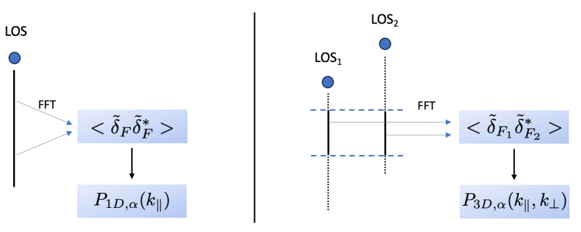
Figure 1: Representation of the fundamental geometric principles behind Ly$\alpha$ correlations for the estimation of $P_{\rm{1}D}$ and $P_{\rm{3}D}$ using a 1D FFT approach. The left panel illustrates the $P_{\rm{1}D}$ measurement, derived from a set of FFTs of independent lines-of-sight (LOS), $\tilde{\delta}_{F}(k_{\parallel})$. Conversely, the right panel illustrates the $P_{\rm{3}D}$ measurement, obtained by correlating 1-dimensional FFTs, namely $\tilde{\delta}_{F_{1}}$ and $\tilde{\delta}_{F_{2}}$, across different lines-of-sight. This illustration also highlights, through bold lines, the delineation of “chunks” within Ly$\alpha$ forests, which serve as the basis for correlating distinct FFTs.

From a technical standpoint, $P_{\rm{3}D}$ determines correlations between pixels taken from distinct quasar spectra, as illustrated in Fig. 1. On the other hand, $P_{\rm{1}D}$ is obtained by correlating pixels belonging to the same quasar spectrum. It is therefore defined as the Fourier transform of the 1-dimensional correlation function $\langle\delta(\boldsymbol{\theta},\lambda_{i})\delta(\boldsymbol{\theta},\lambda_{j})\rangle$ at fixed $\boldsymbol{\theta}$. It is worth noting that the $P_{\rm{1}D}$ can be expressed as a function of the $P_{3D}(z,k_{\perp},k_{\parallel})$ in this manner:

$$P_{\rm 1D}(z,k_{\parallel})=\int\frac{d^{2}k_{\perp}}{(2\pi)^{2}}\;P_{\rm 3D}(z,k_{\perp},k_{\parallel})$$ (2.4)

2.1 The cross-spectrum

The key element in the approach we propose to measure the $P_{\rm{3}D}$, is to first consider a hybrid quantity between real and Fourier space, referred to as the cross-spectrum $P_{\times}(z,\theta,k_{\parallel})$. Similarly to $P_{\rm{3}D}$, $P_{\times}$ quantifies longitudinal correlations in Fourier space. However, for transverse correlations, instead of being expressed in terms of the perpendicular wavenumber $k_{\perp}$, the cross-spectrum resembles a correlation function, being defined as a function of the real-space angular separations $\theta$ between the correlated pixels. To our knowledge, $P_{\times}$ was first introduced in the context of the Ly$\alpha$ forest by [43], and also studied in [63, 64, 62]. Here, we use the same notation $P_{\times}$ as in [43, 62]. However, let us emphasize that $P_{\times}$ is unrelated to the full Fourier space power spectrum computed from the cross-correlations between two distinct fields. $P_{\times}$ can be expressed both as a function of $\xi_{3D}$ or $P_{\rm{3}D}$ in the following way:

$$P_{\times}(z,\theta,k_{\parallel}) \equiv \int\;d\Delta\lambda\;e^{i\Delta\lambda k_{\parallel}}\;\xi_{3D}(z,\theta,\Delta\lambda)$$ (2.5)

$$= \int\frac{d^{2}k_{\perp}}{(2\pi)^{2}}\;e^{i\boldsymbol{\theta}\cdot\mathbf{k_{\perp}}}\;P_{3D}(z,k_{\perp},k_{\parallel})$$ (2.6)

The symmetries of the problem, and the assumption that $z$ is fixed, ensure that $P_{\times}$ is a real quantity. Then, $P_{\rm{1}D}$ as defined in Eqn. 2.4, can be seen as a special case of $P_{\times}$, for null angular separation:

$$P_{1D}(z,k_{\parallel})=P_{\times}(z,\theta=0,k_{\parallel})$$ (2.7)

$P_{\times}$ is a correlator well-adapted to the geometry of Ly$\alpha$ forest observations. The measured Ly$\alpha$ absorption “pixels” are aligned along individual lines-of-sight, usually on a common dense grid of wavelengths: this makes it easy to use the Fourier representation along the parallel direction. On the other hand, the lines-of-sight are sparsely and inhomogeneously distributed in sky coordinates, so that a real-space representation of their correlations is more straightforward.

Defining $\tilde{\delta}(\boldsymbol{\theta}_{i},k_{\parallel})$ as the Fourier transform of each individual line-of-sight $\delta({\boldsymbol{\theta}_{i}},\lambda)$, the definition given by Eqn. 2.5 implies that:

$$\left<\tilde{\delta}(\boldsymbol{\theta}_{i},k_{\parallel})\;\tilde{\delta}^{*}(\boldsymbol{\theta}_{j},k_{\parallel}^{\prime})\right>=2\pi\;\delta^{D}(k_{\parallel}-k_{\parallel}^{\prime})\;P_{\times}(\theta,k_{\parallel})$$ (2.8)

where $\delta^{D}$ is the Dirac delta function and $\theta$ again represents the angular separation between the $\boldsymbol{\theta}_{i}$ and $\boldsymbol{\theta}_{j}$ directions.

2.2 A fast and simple estimator for $P_{\times}$

Considering Eqn. 2.8, it becomes evident that we can expand the 1-dimensional FFT approach, which has already been employed to compute $P_{\rm{1}D}$ as seen in [17, 19], to also compute $P_{\times}$.

In practice, the starting quantity for our $P_{\times}$ measurement at a given redshift $z$, is a set of density contrasts $\delta(\boldsymbol{\theta_{i}},\lambda)$, extracted from the quasars’ Ly$\alpha$ forests in a data sample. Importantly, we assume here that all the $\delta_{i}$ are tabulated on a common regular wavelength grid:

• A common wavelength binning, which is the case of spectra published e.g. by SDSS and DESI. If this is not achieved, one would additionally need to handle phase shifts in the $\tilde{\delta}_{i}\,\tilde{\delta}^{*}_{j}$ products.

• A common wavelength range, centered at $(1+z)\,\lambda_{\alpha}$: indeed, for each pair of lines-of-sight $(i,j)$, the wavelength ranges of $i$ and $j$ must be the same to compute the products of Fourier transforms.

A consequence of these requirements is that only a fraction of each quasar’s Ly$\alpha$ forest is used, depending on each quasar’s redshift, as illustrated in Fig. 1. This, results in a loss of statistics. However, such a choice was not needed in the case of $P_{\rm{1}D}$, e.g. in [17] the density contrasts $\delta_{i}$ were computed on “chunks” of Ly$\alpha$ forests defined in each quasar’s rest-frame, so that all the selected Ly$\alpha$ forest samples contributed to the measurement.

Employing a Fast Fourier Transform method, we initially perform a 1-dimensional Fourier transform on all density fields: $\delta(\boldsymbol{\theta_{i}},\lambda)=\delta_{i}(\lambda)\xrightarrow{FFT}\tilde{\delta}(\boldsymbol{\theta_{i}},k_{\parallel})=\tilde{\delta}_{i}(k_{\parallel})$. Following this, we calculate the angular separations $\theta_{ij}$ for all possible pairs of lines-of-sight $(i,j)$, and we bin these angular separations, depending on the angular separation values for which we intend to calculate $P_{\times}$: an accurate determination of $P_{\times}$ is possible only if there is a sufficient number of line-of-sight pairs within each respective bin. For each selected bin, we define the average angular separation $\theta$ as the mean value of $\theta_{ij}$ corresponding to the pairs that contribute to that specific bin. For a given angular separation bin, considering the sample of line-of-sight pairs $(i,j)$ falling in this specific bin, we compute all products of 1-dimensional FFTs, $\tilde{\delta}_{i}\,\tilde{\delta}^{*}_{j}$. Subsequently, by averaging over all pairs, one can obtain an estimate of $P_{\times}$, as outlined in Eqn. 2.8. We define our estimator:

$$P_{\times}(\theta,k_{\parallel})=\left<\Re\left(\tilde{\delta}_{i}(k_{\parallel})\;\tilde{\delta}_{j}^{*}(k_{\parallel})\right)\right>$$ (2.9)

Since $P_{\times}$ is real, the average of the imaginary parts of $\tilde{\delta}_{i}\tilde{\delta}_{j}^{*}$ products is zero: therefore, to reduce statistical fluctuations we only consider their real parts, $\Re(\tilde{\delta}_{i}\tilde{\delta}_{j}^{*})$, in Eqn 2.9. This is equivalent to including both $(i,j)$ and $(j,i)$ pairs in the averaging process. In the special case of identical line-of-sight pairs $(i,i)$, i.e. $\theta$ = 0, this product simplifies to computing the average of $|\delta_{i}|^{2}$, which corresponds to the conventional FFT estimator for $P_{\rm{1}D}$. As for $P_{\rm{1}D}$, a set of $P_{\times}(\theta,k_{\parallel})$ can be computed separately for different redshift bins, using only Ly$\alpha$ pixels centered around a mean redshift $\langle z\rangle$.

The parallel wavenumbers $k_{\parallel}$ are dictated by the (common) wavelength grid. In this context, we assume a constant pixel size, which can be either $\Delta\lambda_{\rm pix}$ in Å, or $\Delta\log\lambda_{\rm pix}$. Defining the number of pixels $N_{\rm pix}$, the minimum non-zero wavenumber is $\frac{2\pi}{N_{pix}\;\Delta\lambda_{\rm pix}}$. Its maximum value equals the Nyquist frequency $\frac{\pi}{\Delta\lambda_{\rm pix}}$.

We derive the statistical error bars and covariance for $P_{\times}$ within a specific angular separation bin, using the dispersion of individual $\delta_{i}\delta_{j}$ measurements. This is identical to the way it is done for $P_{\rm{1}D}$ [17]. The underlying assumption is that individual pair measurements $(i,j)$ are independent of each other. This assumption holds in the context of this study, because we are considering small angular separations and using relatively low-density Ly$\alpha$ observations over a substantial portion of the sky: the probability for a line-of-sight $(i)$ to contribute to two pairs $(i,j)$ and $(i,j^{\prime})$ within the same angular separation bin is quite low. Due to the same reason, we anticipate that the statistical covariance of $P_{\times}$ will be minimal between different angular separation bins. Consequently, it is not taken into account in this study. It is important to note that if a future work expands the measurement of $P_{\times}$ to larger angular separations, a more refined estimation of the covariance would be essential.

In terms of computational requirements, this method demands very limited resources. Some computation time is needed to tabulate pairs of lines-of-sight as a function of angular separations. The subsequent step, which involves computing 1D FFTs for all individual lines-of-sight, requires a computation time identical to the case of $P_{\rm{1}D}$. Overall, as an example, our computations indicate that it takes only a few minutes, when executed on a single CPU node of the Perlmutter machine at the NERSC computing center, to compute $P_{\times}$ in a single redshift bin, for the SDSS sample considered in Section 4.

2.3 Noise and resolution

When dealing with real data, given that we are interested in small-scale correlations, the main instrumental effects that need to be corrected for are the spectroscopic resolution and its noise. Although such corrections depend on the considered data set, they are relatively similar between different instruments. We consider here the case of SDSS spectra, since we later apply our method to SDSS data sets.

The expression of the measured density contrast for a line-of-sight $i$, $\delta_{i}(\lambda)$, can be written as a function of the “astrophysical” contrast $\delta_{i,{\rm Ly\alpha}}(\lambda)$ as follows:

$$\delta_{i}(\lambda)=\delta_{i,{\rm Ly\alpha}}(\lambda)\ast W_{i}(\lambda,R)+\delta_{i,n}(\lambda)$$ (2.10)

In this expression, $\delta_{i,{\rm Ly\alpha}}$ is convolved by the kernel function $W_{i}(\lambda,R)$ that accounts for the spectral response of the spectrograph, as well as the sample’s wavelength pixelization. Its main parameter is the resolution $R$, which is specific to the measured spectrum. $\delta_{i,n}(\lambda)$ represents noise fluctuations: those are usually well represented by a Gaussian white noise model, whose amplitude depends on the considered spectrum. In Fourier space, Eqn. 2.10 becomes:

$$\tilde{\delta}_{i}(k_{\parallel})=\tilde{\delta}_{i,{\rm Ly\alpha}}(k_{\parallel})\times\widetilde{W}_{i}(k_{\parallel},R)+\tilde{\delta}_{i,n}(k_{\parallel})$$ (2.11)

We define $P_{\times,{\rm Ly\alpha}}$ and $P_{\times}$ as the cross-spectra of $\delta_{\rm Ly\alpha}(\boldsymbol{\theta},\lambda)$ and $\delta(\boldsymbol{\theta},\lambda)$ respectively. We also define the noise (cross) power spectrum in the following way:

$$P_{n}(\theta,k_{\parallel})=\langle\Re(\tilde{\delta}_{i,n}\tilde{\delta}^{*}_{j,n})\rangle\$$ (2.12)

In this expression, similarly to previous expressions, $(i,j)$ pairs are separated by $\theta$. It is then straightforward to derive $P_{\times,{\rm Ly\alpha}}$ from the observed $P_{\times}$, by employing an equation that is an extension of the one used for $P_{\rm{1}D}$, e.g. in [17]:

$$P_{\times,\rm Ly\alpha}(\theta,k_{\parallel})=\frac{P_{\times}(\theta,k_{\parallel})-P_{n}(\theta,k_{\parallel})}{\left<\widetilde{W}_{i}(k_{\parallel})\,\widetilde{W}_{j}(k_{\parallel})\right>}$$ (2.13)

Since the noise is independent of the Ly$\alpha$ signal, all $\langle\tilde{\delta}_{i,n}\tilde{\delta}_{j,{\rm Lya}}^{*}\rangle$ vanish. If we neglect the impact of correlated noise between different measured spectra, we have $\langle\tilde{\delta}_{i,n}\tilde{\delta}^{*}_{j,n}\rangle=0$ for any pair $(i,j)$ of lines-of-sight with $i\neq j$. We will come back to this assumption in the specific case of SDSS spectra in Section 4.2. In that case, the only non-zero noise correlation terms are for $i=j$, therefore we have:

$$P_{n}(\theta,k_{\parallel})=\begin{cases}\langle|\tilde{\delta}_{i,n}|^{2}\rangle&\text{if $\theta=0$}\\ ~{}~{}~{}~{}0&\text{if $\theta>0$}\\ \end{cases}$$ (2.14)

Hence, contrarily to the case of $P_{\rm{1}D}$, there is no noise correction to apply for $\theta>0$.

2.4 From $P_{\times}$ to $P_{3D}$

The measurement of $P_{\times}$ itself is of interest, and as we will emphasize in the conclusion, it could certainly be directly used for cosmological inferences within a full modeling approach. However, the computation of $P_{\times}(z,\theta,k_{\parallel})$ also allows one to infer $P_{\rm{3}D}$. Using Eqn. 2.3, we have:

$$P_{\rm 3D}(z,k_{\perp},k_{\parallel})=\int d^{2}\theta\;e^{i\boldsymbol{\theta\cdot k_{\perp}}}\;P_{\times}(z,\theta,k_{\parallel})$$ (2.15)

Moving to cylindrical coordinates, the angular symmetry of $P_{\times}$ permits this 2D integral to be simplified to a 1D integral:

$$P_{\rm 3D}(z,k_{\perp},k_{\parallel})=2\pi\int_{0}^{\infty}d\theta\,J_{0}(k_{\perp}\theta)\,\theta\,P_{\times}(z,\theta,k_{\parallel})$$ (2.16)

Here $J_{0}(x)$ is a first kind Bessel function of order zero, which oscillates while slowly decreasing as a function of $x=k_{\perp}\theta$.

Following Eqn. 2.16, one straightforward approach for inferring $P_{\rm{3}D}$ involves performing numerical integration of $P_{\times}$, which is the technique used in this work. Numerically, since $P_{\times}$ is expected to be a smooth function of $\theta$ for the scales of interest, we perform an interpolation of $P_{\times}$ over a finely-spaced grid of $\theta$ values, using a smoothing spline fit. This ensures that we accurately capture the oscillations of the Bessel function $J_{0}(x)$. Using the interpolated cross-spectrum, we perform the numerical integration using Eqn. 2.16. This integration can be done only for certain values of $k_{\perp}$ and $k_{\parallel}$. First of all, $\theta_{\rm min}$, the smallest non-zero angular separation for which we measure $P_{\times}$, dictates the largest perpendicular mode $k_{\perp,{\rm max}}\propto 1/\theta_{\rm min}$. In addition to that, the numerical integration makes sense only if typical variations of $P_{\times}$ as a function of $\theta$ take place on scales larger than $\theta_{\rm min}$. In practice, $P_{\times}$ is a rapidly decreasing function of $\theta$ since it is a correlation function as a function of transverse coordinates. Therefore, a simple and somewhat arbitrary criterion we choose is to require that $P_{\times}(\theta_{\rm min})/P_{\times}(\theta=0)>0.3$. Given that $P_{\times}$ decreases faster with $\theta$ for larger values of $k_{\parallel}$, this results in a maximal value $k_{\parallel,{\rm max}}$. Using a simple toy model for $P_{\times}$, we estimate that the systematic error on $P_{\rm{3}D}$ due to the finite value of $\theta_{\rm min}$ is of the order of 20 %, with this criterion and our chosen integration method.

Within this method, the $P_{\rm{3}D}$ statistical uncertainties are propagated following a simple Monte-Carlo approach. Initially, random realizations of $P_{\times}$ are drawn according to the measured $P_{\times}$ covariance matrix. Subsequently, the statistical errors on the measured $P_{\rm{3}D}$ are given by the dispersion of the random $P_{\rm{3}D}$ values obtained after numerical integration of the random $P_{\times}$ realizations, according to Eqn. 2.16 as well.

It is evident that there exist more advanced approaches for estimating $P_{\rm{3}D}$, such as implemented in [62]. This will be discussed later in the conclusion. Here we use our simple numerical integration due to the fact that the choice of an alternative $P_{\rm{3}D}$ estimator depends on the strategy used to physically interpret the measurement - a step that we leave for a future work. We emphasize that regardless of the chosen method, the derivation of $P_{\rm{3}D}$ from $P_{\times}$ demands negligible computational resources in comparison to the $P_{\times}$ computation itself. Additionally, we highlight that the numerical integration approach is completely model-independent, which is not the case for other approaches such as the quadratic estimator used in [62], in which $P_{\rm{3}D}$ is parameterized using an expansion around a reference model, or even more using explicit fitting functions such as those of [60].

Units

• When modelling the Ly$\alpha$ forest, for example in the case of simulated data derived from hydrodynamical simulations detailed in Section 3, with a known background cosmology, $P_{\times}$ and $P_{\rm{3}D}$ are computed in $h^{-1}$Mpc and [$h^{-1}$Mpc]³ respectively. Angular separations $\theta$ are also expressed in $h^{-1}$Mpc. This allows one to compare measured power spectra to the “truth” power spectra of the simulations, whose coordinates are given in comoving Mpc.

• When using real data, it is more appropriate to provide a cosmology-independent measurement, that can be later interpreted within any cosmological model. As already mentioned in Section 2, depending on whether the pixel size along lines-of-sight is expressed in Å or in km s^-1 (in the case of a log scale wavelength grid), $P_{\times}$ is expressed in Å or km s^-1 units, and $P_{\rm{3}D}$ is expressed in [deg² Å] or in [deg² km s^-1].

For reference, in the case of a flat cosmological model with comoving distance $D_{c}(z)$ in Mpc, and Hubble rate $H(z)$ in km s^-1 Mpc^-1, and for data sets at mean redshift $z$, with $c$ in km s^-1 and $\lambda_{\alpha}$ in Å, the conversion formulae are:

$$P_{\times}[h^{-1}\mathrm{Mpc}] = \frac{hc}{\lambda_{\alpha}~{}H(z)}~{}P_{\times}[\text{\AA}]$$ (2.17)

$$P_{\times}[\mathrm{km~{}s^{-1}}] = \frac{c}{\lambda_{\alpha}~{}(1+z)}~{}P_{\times}[\text{\AA}]$$ (2.18)

$$P_{\rm 3D}[h^{-1}\mathrm{Mpc}]^{3} = \left(\frac{\pi}{180}\right)^{2}\frac{h^{3}\,c}{\lambda_{\alpha}}\frac{D_{c}(z)^{2}}{H(z)}~{}P_{\rm 3D}[\mathrm{deg^{2}}~{}\text{\AA}]$$ (2.19)

3 Validation with hydrodynamical simulations

In this section, we apply the previously outlined method to simulated Ly$\alpha$ absorption fields. We make use of the output of a cosmological simulation, run with the Nyx software. This provides tests of our measurement strategy with a realistic Ly$\alpha$ forest model, and more importantly, a well-defined input $P_{\rm{3}D}$.

3.1 Description of the simulations

Simulated Ly$\alpha$ forest samples have been generated over large volumes such as those covered by large spectroscopic surveys, e.g. in [65, 66]. However, such mock samples are optimized to mimic large-scale correlations, and do not necessarily reproduce a well-defined small-scale $P_{\rm{3}D}$ of the Ly$\alpha$ absorption field. On the other hand, using a simple Gaussian random field with a known $P_{\rm{3}D}$ may be unrealistic, since at small scales, the Ly$\alpha$ absorption field is highly non-Gaussian. We therefore resort to the use of Ly$\alpha$ absorption fields as computed by cosmological hydrodynamical simulations. Currently, these simulations cannot span over a cosmological volume equivalent to the one probed by BOSS, but we can compensate for this limitation by drawing lines-of-sight inside the simulation box with an appropriate density, ensuring that the statistics of relatively small-separation pairs reasonably matches that of real data.

Nyx [67, 68] is a cosmological simulation code, solving the evolution of the baryonic gas coupled to dark matter in the expanding Universe. While dark matter is treated with an N-body approach, the gas hydrodynamics are solved on a mesh. Nyx is particularly well adapted to model the Ly$\alpha$ forest, as described in details in [5], and applied in e.g. [69, 59]. The Eulerian, fixed-mesh algorithm turns out to be efficient to model the small-scale fluctuations of baryon properties in the low-density regions of the cosmic web, where most of the Ly$\alpha$ absorption signal is produced. The Ly$\alpha$ forest modelling is done by following electrons, hydrogen and helium species (neutral and ionized), making use of relevant atomic, heating and cooling processes. Concerning the post-processing of a Nyx simulation, this is done using the Gimlet software [70]. Gimlet is a C++, MPI-parallel toolkit well adapted to Nyx outputs [5].

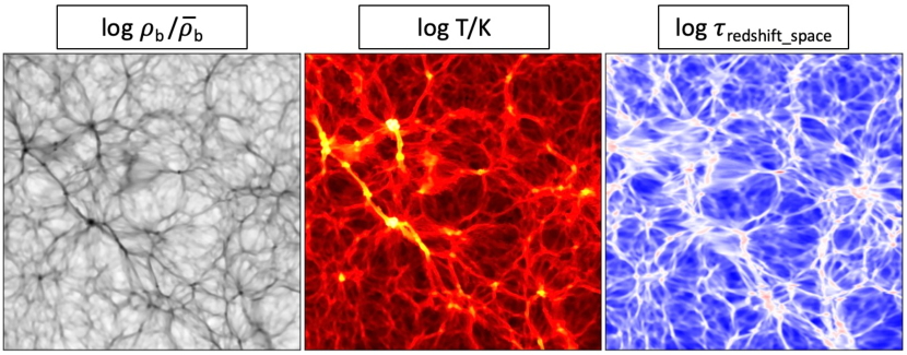
Figure 2: Slice of the baryon density, temperature, and optical depth in redshift space from the employed Nyx simulation, with 1536³ cells and box size of 150 $h^{-1}$Mpc. The baryon density and temperature fields are statistically isotropic. For the optical depth field, the horizontal axis corresponds to the line-of-sight: the effects of IGM temperature, peculiar velocities and redshift space distortions result in anisotropies of its statistical properties.

Here we make use of an output (snapshot) from a Nyx simulation that is described in more details in [71]. The simulation was run starting from $z=200$, with Zel’dovich initial conditions, and cosmological parameters from [72]: $\Omega_{b}=0.0487$, $\Omega_{m}=0.31$, $H_{0}=67.5$, $n_{s}=0.96$ and $\sigma_{8}=0.83$. Importantly for the Ly$\alpha$ forest, a spatially uniform UV+X-ray radiation field is assumed to dictate the ionization state of Hydrogen and Helium, following the middle reionization scenario of [73]. The simulated cosmological volume is a large cubic box, $150$ $h^{-1}$Mpc wide, with $1536^{3}$ gas cells, resulting in a resolution of $98$ $h^{-1}$kpc. This volume is large enough to draw lines-of-sight with an appropriate number density. Additionally, the spatial resolution is good enough to physically capture some of the relevant small-scale features in the Ly$\alpha$ forest. Note that it is not enough to fully resolve the Jeans scale $\lambda_{J}\sim 80$ $h^{-1}$kpc, but this is not important for this study: the minimum non-zero angular separation bin $\theta_{\rm min}$ we use in mocks with a “realistic” line-of-sight density, and with SDSS data, corresponds to transverse distances $\sim 0.6$ $h^{-1}$Mpc, much larger than $\lambda_{J}$. For practical reasons we use the simulation output at redshift $z=2.0$.

The IGM’s Ly$\alpha$ optical depth $\tau_{\alpha}$ is numerically calculated in redshift space from simulation outputs using Gimlet, which takes into account a Gaussian thermal line broadening. A slice of $\tau_{\alpha}$, computed in redshift space with respect to the line-of-sight, is shown on the right-hand side of Fig. 2. We also show the corresponding baryon density and temperature fields, that were used to compute $\tau_{\alpha}$. These density and temperature fields are statistically isotropic. Nonetheless, the effects of thermal broadening, peculiar velocities and redshift space distortions have a clear impact on $\tau_{\alpha}$, resulting in statistical anisotropies in this field, with a preferred axis given by the line-of-sight.

3.2 Mock generation

In order to validate our measurement approach, we generate mock line-of-sight samples from the simulations described in Section 3.1 and perform measurements of $P_{\times}$ and $P_{\rm{3}D}$. Starting with the computed $\tau_{\alpha}$ grid, we derive the transmitted flux fraction grid, $F(\lambda)=e^{-\tau_{\alpha}}$. Additionally, we compute the corresponding grid of density contrasts $\delta$ based on Eqn. 2.1. Following this, a 3D Ly$\alpha$ absorption power spectrum $P_{\rm{3}D}$ is computed using Gimlet, which relies numerically on a 3D FFT, well-adapted to the regularly-gridded $\delta$ field. We later refer to this $P_{\rm{3}D}$ as the “truth”, although it is essential to acknowledge that this power spectrum is also altered by numerical effects, stemming from the FFT process, as well as the effect of cosmic variance due to the finite box size.

Line-of-sight mock samples are finally generated from the $\delta$ grid. To create them, we initially select random floating-point values for the $x$ and $y$ coordinates of each line-of-sight, and subsequently determine the corresponding $\delta$ values along the z-axis. To be more precise, the $\delta$ of each line-of-sight of random $x$ and $y$ coordinates is obtained through a linear interpolation on the $\delta$ grid. This method ensures that the lines-of-sight are randomly distributed, even when dealing with small angular separations. By construction, the pixels of individual lines-of-sight are all on the same grid, with a $98$ $h^{-1}$kpc pixel size.

3.3 Results with a reference, high-density and noiseless mock

As a first validation of our pipeline, we build a reference mock sample with $10^{4}$ lines-of-sight, which does not include noise nor resolution effects. To compute $P_{\times}$ on this mock, we follow the procedure outlined in Section 2. First, after having computed the angular separations of all possible line-of-sight pairs in our sample, we choose angular separation bins centered at $\langle\theta\rangle=$ 0^∘ (case of $P_{\rm{1}D}$), 0.0015^∘, 0.0045^∘, 0.008^∘, followed by a regular binning of width 0.01^∘ ranging from 0.015^∘ to 0.35^∘, and finally the two bins 0.45^∘ and 0.55^∘. The maximum considered value is 0.55^∘, which corresponds to $\sim 35$ $h^{-1}$Mpc, much smaller than the size of the simulation box. Then, for each angular separation bin, we proceed with the measurement of $P_{\times}(\theta,k_{\parallel})$ which represented in Fig. 3 for selected angular separation bins.

Figure 3: Estimated $P_{\times}$$(\theta,k_{\parallel})$ from our reference mock of $10^{4}$ noiseless lines-of-sight drawn from the 150 $h^{-1}$Mpc Nyx box at z = 2.0. $P_{\times}(k_{\parallel},\theta=0)$ being the $P_{\rm{1}D}$, is compared to the “truth” $P_{\rm{1}D}$ provided by Gimlet and represented by a continuous blue line. We rebinned $P_{\times}$ values on a logarithmic grid in $k_{\parallel}$. Error bars indicate statistical uncertainties.

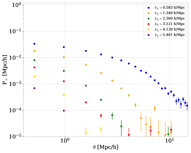
Figure 4: Same as Fig. 3, but representing $P_{\times}$ as a function of angular separation $\theta$, i.e. highlighting the fact that $P_{\times}$ is a correlation function as a function of transverse separation. Notably, the transverse correlations in the $\delta$ field decrease faster as a function of $\theta$ when considering short-wavelength longitudinal modes (large $k_{\parallel}$) with respect to long-wavelength modes.

Initially, we checked that the measured $P_{\times}(k_{\parallel}\,|\,\theta=0)$ is in agreement with the “truth” $P_{\rm{1}D}$ computed by Gimlet. For $\theta>0$, the shape of $P_{\times}(k_{\parallel})$ is similar to $P_{\rm{1}D}$; however when $\theta$ increases, the overall power decreases, and the small-scale (high $k_{\parallel}$) attenuation takes place at smaller values of $k_{\parallel}$. In order to highlight this feature, Fig. 4 shows the same measurement, but as a correlation, i.e. as a function of $\theta$: as expected and already highlighted in e.g. [63], the transverse correlations in the $\delta$ field decrease faster when considering short-wavelength longitudinal modes (large $k_{\parallel}$) with respect to long-wavelength modes.

We then derive $P_{3D}(k_{\perp},k_{\parallel})$, for values of $k_{\perp}$ identical to those tabulated in the “truth” $P_{\rm{3}D}$ computed by Gimlet. Fig. 5 presents the computed $P_{\rm{3}D}$ for selected $k_{\perp}$ values ranging from $\sim 0.1$ to $\sim 10\,h\,{\rm Mpc}^{-1}$, as well as the corresponding “truth”. The agreement between both estimations is very good: this validates our method to estimate $P_{\rm{3}D}$ for a large range of $(k_{\perp},k_{\parallel})$. In this ideal setup, the number of line-of-sight pairs used to compute $P_{\times}$ is huge, leading to remarkably small statistical error bars. Nonetheless, it is noteworthy that our $P_{\rm{3}D}$ estimator exhibits reduced precision for $k_{\perp}\gtrsim 10\,h\,{\rm Mpc}^{-1}$. This maximal value of $k_{\perp}$ is dictated by the smallest angular separation bin $\theta$.

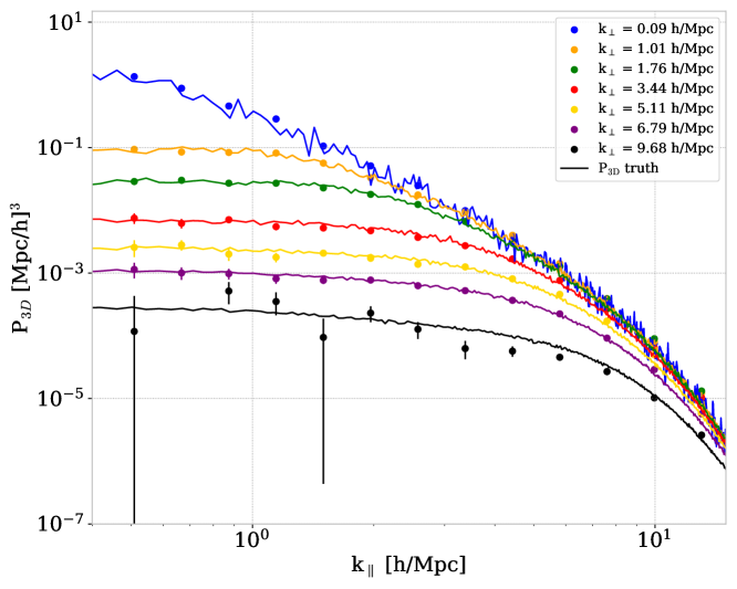
Figure 5: Estimated $P_{\rm{3}D}$$(k_{\perp},k_{\parallel})$ from our reference mock of $10^{4}$ noiseless lines-of-sight within the 150 $h^{-1}$Mpc Nyx box at $z=2$. Continuous lines show the “truth” $P_{\rm{3}D}$ provided by Gimlet, estimated by full 3D FFT of the box field. As in Fig. 3, we rebinned our $P_{\rm{3}D}$ values on a logarithmic grid in $k_{\parallel}$, and error bars represent statistical uncertainties.

In order to physically interpret the measured $P_{\rm{3}D}$, we perform a change of coordinates from Cartesian $(k_{\perp},k_{\parallel})$ to polar $(k=\sqrt{k_{\perp}^{2}+k_{\parallel}^{2}},\mu=k_{\parallel}/k)$. We then compute the ratio of $P_{\rm{3}D}$ to the (known) linear matter power spectrum $P_{\rm L}(k,z=2)$ estimated by the CLASS Boltzmann solver [74]. This recast of the measurement is shown in Fig. 6. In order to highlight its interpretation, we fit these points with the analytic function given by Eqn. 3.6 of [60]:

$$\frac{P_{\rm 3D}(k,\mu)}{P_{\rm L}(k)}=b^{2}\,(1+\beta\mu^{2})^{2}\,\exp\left((q_{1}\Delta^{2}(k)+q_{2}\Delta^{4}(k))\left[1-\left(\frac{k}{k_{v}}\right)^{a_{v}}\mu^{b_{v}}\right]-\left(\frac{k}{k_{p}}\right)^{2}\right)$$ (3.1)

In this expression $\Delta^{2}(k)=k^{3}P_{\rm L}(k)/2\pi^{2}$. At low $k$, $P_{\rm{3}D}$ is in a near-linear regime: its amplitude is dictated by the bias $b$ and its $\mu$ dependence is driven by the linear RSD term $(1+\beta\mu^{2})^{2}$. Then, the isotropic boost of the power spectrum due to non-linear gravitational growth is parameterized by the $q_{1}$ and $q_{2}$ terms. Line-of-sight broadening produced by peculiar velocities and the IGM temperature generates a strongly $\mu$-dependent cutoff in $P_{\rm{3}D}$ ($k_{v}$, $a_{v}$, $b_{v}$ terms). Finally, at large $k$, the impact of Jeans smoothing is isotropic, modelled by the $\exp-(k/k_{p})^{2}$ term. The parameters we derive from our fit are $(b,~{}\beta,~{}q_{1},~{}q_{2},~{}k_{v},~{}a_{v},~{}b_{v},~{}k_{p})=(0.043,~{}1.7,~{}2.3,~{}-0.5,~{}5.3,~{}0.42,~{}1.16,~{}9.4)$. Importantly, the recovered $P_{\rm{3}D}$ is in good agreement with the simulation’s truth, also displayed in Fig. 6. We notice that for relatively low $k\sim 1.5-4$ $h^{-1}$Mpc, our measurement systematically overestimates $P_{\rm{3}D}$ for large $\mu$, and underestimates $P_{\rm{3}D}$ for low $\mu$. This generates a bias on several parameters when fitting Eqn. 3.1. Still, we compared the fit results from our measurement to those from gimlet’s “truth”, and found that all parameters are within $1.1\,\sigma$. More importantly, we also observe that even in the case of this reference mock sample, the statistical error bars are large when it comes to measure $P_{\rm{3}D}$ for small values of $\mu\lesssim 0.3$. This is again related to the limited statistics of very small-separation pairs of lines-of-sight. In spite of these limitations, it is clear that our $P_{\rm{3}D}$ measurement from this reference mock allows to disentangle between the different effects included in the model of Eqn. 3.1 - hence improving our interpretation of Ly$\alpha$ data, both in terms of precision and robustness.

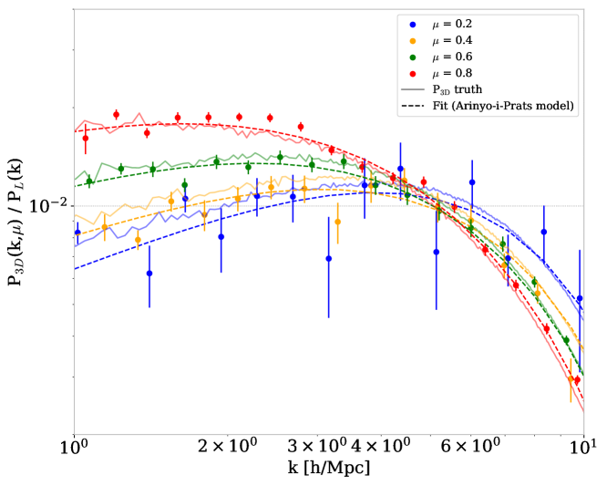
Figure 6: Ratio of $P_{\rm{3}D}$$(k,\mu)$ to the linear matter power spectrum $P_{\rm L}(k)$, computed for 4 values of $\mu=k_{\parallel}/k$ and as a function of $k=\sqrt{k_{\parallel}^{2}+k_{\perp}^{2}}$. Points with error bars represent the measured $P_{\rm{3}D}$ from our reference mock, which is also shown in Fig. 5, but in a different coordinate system. Continuous thin lines represent the simulation “truth” similarly to Fig. 5. Dashed lines are the result of an 8-parameter fit of the measurement points to Eqn. 3.1, as described in the text.

3.4 Results with realistic mocks

In this section, we assess the performance of our measurement approach using realistic mock data sets that resemble existing or forthcoming large spectroscopic quasar samples. We specifically take into consideration two crucial factors that inevitably influence the accuracy of our measurements: instrumental noise and lines-of-sight statistics. A study involving more realistic mocks which encompass elements such as astrophysical contaminants and more detailed instrumental effects, falls beyond the scope of this article.

We first construct a mock sample with the same line-of-sight statistics as in the reference mock discussed in Section 3.3. However, we inject noise into the measured Ly$\alpha$ density contrast $\delta$. This noise component is an uncorrelated, Gaussian white noise with standard deviation $\sigma_{\delta}=0.5/\sqrt{\Delta\lambda}$, where $\Delta\lambda$ is the forest pixel size in Å. This particular value aligns with the typical characteristics of SDSS Ly$\alpha$ samples. To derive $P_{\times}$ from this mock sample, we subtract the noise spectrum $P_{n}$ when $\theta=0$, as explained in Section 2.3.

Next, we construct a mock realization with noise-free $\delta$ samples as in the reference mock detailed in Section 3.3. However, in this case, we opt for a reduced number of lines-of-sight, specifically selecting 500 lines-of-sight. We choose this number such that the pairs count at small angular separations resembles those from the SDSS sample given in Table 1 of Section 4. For instance, this mock contains 70 line-of-sight pairs contributing to the angular separation bin $\theta=0.03^{\circ}$, i.e. $\simeq 1.9$ $h^{-1}$Mpc.

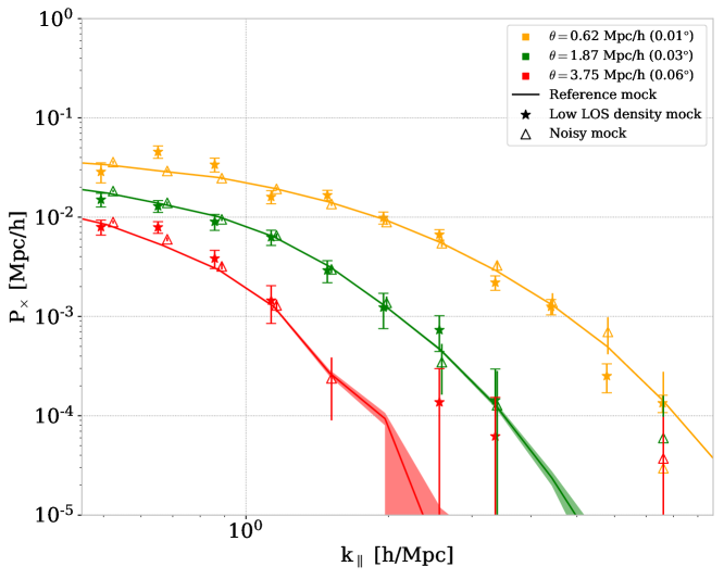
Figure 7: Comparison of $P_{\times}$ measurements from different mock realizations, for 3 angular separation bins. The continuous lines represent $P_{\times}$ from the reference mock, already presented in Fig. 3, with statistical errors shown by shaded bands. Measurements from mocks with noisy data and with a reduced density of lines-of-sight are shown by triangle points and stars, respectively. For visual clarity, data points are slightly shifted along the horizontal axis.

Figure 7 shows a comparative representation of the estimated $P_{\times}$ from these two mock data sets, in contrast to the reference case of Section 3.3, for three distinct angular separation bins centered at $\theta$ = 0.01^∘, 0.03^∘ and 0.06^∘. Comparing the $P_{\times}$ from these more realistic mocks to the reference $P_{\times}$, we notice that the considered effects result in an increase of statistical uncertainties in the measurement. More specifically, for the mock sample with noise, the increase of statistical error bars becomes significant when $P_{\times}$ reaches low values: this is similar to the case of $P_{\rm{1}D}$ for large $k_{\parallel}$. On the other hand, for the mock with less lines-of-sight, the reduced number of pairs, especially at small angular separations, results in large statistical fluctuations for all measured values.

As a result of these mock studies, we conclude that measurements of $P_{\times}$ for $\theta>0$ should be feasible with Ly$\alpha$ data from large surveys, but clearly not at the level of precision of existing $P_{\rm{1}D}$ measurements.

4 Application to SDSS quasar spectra

We now move to the application of the method on the largest currently public Ly$\alpha$ forest data set: the SDSS DR16 quasar spectra. We stress that our goal here is to essentially provide a proof-of-principle of our pipeline from a real, already well-studied Ly$\alpha$ forest sample. We are not looking for the most precise measurement possible from this sample, nor do we attempt any interpretation in terms of IGM physics and cosmology.

4.1 Data sample

The SDSS [75, 76, 77, 78], BOSS [44] and subsequent eBOSS [79] surveys provide the largest publicly available optical spectroscopic data set of extragalactic objects to date. This data set encompasses a large set of Ly$\alpha$ absorption spectra from quasars with redshifts $z>2.1$ and a relatively homogeneous sky distribution spread all over the SDSS footprint, covering approximately 1/4 of the sky.

In our analysis, we select quasars drawn from the eBOSS DR16Q catalog [80], a component of the 16th SDSS data release [81]. Our selection criteria are focused on quasars with redshift $z>2.1$, with no identified broad absorption lines (BAL) nor damped Lyman-$\alpha$ (DLA) features in their spectra.

We measure Ly$\alpha$ forest fluctuations, $\delta(\lambda)$, from the set of quasar spectra, using the continuum fitting algorithm implemented in the picca  code. This code computes $\delta$ from the measured quasar flux $f_{q}(\lambda)$ through:

$$\delta(\lambda)=\frac{f_{q}(\lambda)}{\overline{F}(z)C_{q}(\lambda)}-1$$ (4.1)

In this expression, $\overline{F}(z)$ is the mean IGM transmission at redshift $z=\lambda/\lambda_{\alpha}-1$, as previously defined. $C_{q}$ is the quasar’s unabsorbed flux, called continuum, and assumed to be a universal function of the rest-frame wavelength $\lambda_{\rm RF}$, multiplied by a quasar-dependent correction: $C_{q}=(a_{q}+b_{q}\log\lambda_{\rm RF})\,C(\lambda_{\rm RF})$. The product $\overline{F}(z)C_{q}(\lambda)$ is determined by an iterative fit. The continuum fitting procedure is analogous to the approach employed during the eBOSS P1D measurement in [17]. Specifically, the fitting was done in the rest-frame wavelength range $\lambda_{\rm RF}\in[1050-1180]$ Å. No weights were applied to individual pixel fluxes $f_{q}(\lambda)$. Two types of pixels were masked: those flagged by the SDSS processing pipeline due to e.g. cosmic rays, and those that correspond to observed wavelengths matching atmospheric emissions and galactic absorption lines, identically to [17]. Finally, only spectra with a mean SNR per pixel larger than 1 were used.

The set of $\delta(\lambda)$ obtained from the DR16 sample is similar to the one used in the P1D measurement of [17]. Since no resampling is performed at the stage of continuum fitting, all the $\delta(\lambda)$ are pixelized on the SDSS common wavelength grid, equally spaced in logarithmic scale, with a binning $\Delta\log\lambda_{\rm pix}=10^{-4}$.

Since our measurement is done separately for different redshift bins as already mentioned in Section 2.1, our initial step involves extracting subsets of Ly$\alpha$ forests from the common sample of $\delta$, corresponding to specific redshift bins: for a given redshift $z$, we define a wavelength range $(\lambda_{\rm min}-\lambda_{\rm max})$, centered at $(1+z)\lambda_{\alpha}$ and then, we only select lines-of-sight whose Ly$\alpha$ forest pixels completely overlap this wavelength interval. The width of this interval determines the smallest measurable $k_{\parallel}$. Additionally, lines-of-sight having masked pixels in this wavelength range are discarded. These selections, especially the first one, certainly reduce the statistics. However they greatly simplify the calculation of cross-correlations $\delta_{i}\times\delta_{j}^{*}(k_{\parallel})$ as emphasized in Section 2.2.

As in [16, 17], given that the spectral binning $\Delta\log\lambda_{\rm pix}$ is in logarithmic scale, we tabulate $k_{\parallel}$ in units of km/s, as already described in Section 2.4. The spectroscopic resolution $R$ is derived for each sample using the picca software, identically to [16]: it is taken from the spectroscopic pipeline output, and an analytic correction function is applied, depending on the wavelength and position of the spectrum on the CCD, as described in Section 2.3. This correction varies from 1 to 10 %, and is defined as [16]:

$$W(k_{\parallel},R)=\exp\left(-\frac{1}{2}(kR)^{2}\right)\times\frac{\sin(k_{\parallel}\Delta v/2)}{k_{\parallel}\Delta v/2}$$ (4.2)

4.2 Measurement

We consider here two redshift bins, for which the statistical sample is particularly abundant.

• The bin $z=2.2$: obtained by selecting $(\lambda_{\rm min},\lambda_{\rm max})=(3850,3930)$ Å. It includes 38461 Ly$\alpha$ forests covering this wavelength range, each forest containing 89 pixels, spanning over a comoving distance of $\simeq 59$ $h^{-1}$Mpc.

• The bin $z=2.4$: obtained by selecting $(\lambda_{\rm min},\lambda_{\rm max})=(4056,4210)$ Å. It includes 18653 Ly$\alpha$ forests covering this wavelength range, each forest containing 162 pixels, spanning over a comoving distance of $\simeq 105$ $h^{-1}$Mpc.

The choice of wavelength ranges is made with the intention of aligning the data around the chosen redshift values while ensuring the exclusion of spectral regions contaminated by sky lines and calcium H and K galactic absorption lines. Although the sample at $z=2.2$ offers the largest number of lines-of-sight, the $z=2.4$ sample is less affected by noise and contains more pixels per line-of-sight. The width of these spectral segments is sufficiently broad to enable measurements at $k_{\parallel}\gtrsim 0.002$ km/s.

To compute $P_{\times}$, we select $\delta_{i}$ values based on their mean signal-to-noise per pixel $\overline{\rm SNR}$, to be used in the measurement. For $P_{\times}(\theta>0)$, we require $\overline{\rm SNR}>1$. It is worth noting that this criterion is somewhat less stringent compared to the one employed in [17]. However, our measurement for small, non-zero values of $\theta$, is constrained by limited statistics, and furthermore, noise is expected to have a reduced impact on the cross-correlations between distinct lines-of-sight compared to their auto-correlations. To set this threshold, we scanned over a range of values for the $\overline{\rm SNR}$ threshold and we observed that the average statistical uncertainty in the measured $P_{\times}$ is roughly optimized for the chosen threshold. In the case of $P_{\times}(\theta=0)$, i.e. $P_{\rm{1}D}$, we have more abundant statistics, and in that instance we employ a more strict criterion: $\overline{\rm SNR}>2$. Additionally, in previous works [16, 17], a threshold was applied to each line-of-sight’s mean spectroscopic resolution, $\overline{R}>85$ km/s. We evaluated the impact of such a threshold on our measurements and found it to be small in comparison to our statistical uncertainties for $\theta>0$. Therefore, we apply this threshold only for $P_{\times}(\theta=0)$ in our study. Finally, when we compute the $P_{\times}$, we take into consideration both uncorrelated noise and resolution effects, following the procedures detailed in Section 2.3.

The cross-spectra measured in the redshift bins $z=2.2$ and 2.4 are given in Fig. 8. The error bars represent only statistical uncertainties. The published measurement of $P_{\rm{1}D}$ from eBOSS [17], depicted in dotted lines, can be compared to our estimation of $P_{\times}(\theta=0)$. A discrepancy is observed at small values of $k_{\parallel}$, and this is expected due to several factors. To start with, we did not implement a correction due to the continuum fitting. Additionally, we used the SDSS DR16 data set, whereas [17] relied on the DR14 data set. Furthermore, we employed a different DLA catalog for masking. Lastly, our measurement includes absorption features from the Ly$\alpha$ forest, along with a subdominant contribution from metals that we have not accounted for: metal correlations were subtracted using sideband data in [17], resulting in $\lesssim 10$ % corrections.

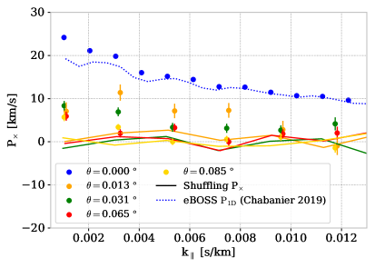
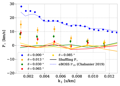
Figure 8: $P_{\times}$ measurement from SDSS DR16 data at mean redshifts $z=2.2$ (left) and $z=2.4$ (right). Data points are rebinned as a function of $k_{\parallel}$ for $\theta>0$. Error bars are statistical only. The dotted line represents the published $P_{\rm{1}D}$ measurement by [17], which includes several additional systematic corrections. Continuous lines represent a null test carried out by shuffling angular coordinates of individual lines-of-sight. Note that the inverse of a pixel size in the original SDSS spectra is $0.0145$ in s/km unit.

The angular separation bins used to compute $P_{\times}$, together with their associated pair statistics, are given in Table 1. The lowest bin is $\theta_{\rm min}=0.013^{\circ}$. The comparison between the small number of pairs used to compute $P_{\times}$ at small non-zero angular separations and the case where $\theta=0$ ($P_{\rm{1}D}$), highlights how challenging this measurement is.

$\langle\theta\rangle(^{\circ})$	0	0.013	0.03	0.065	0.085
$N(z=2.2)$	6848	105	329	342	440
$N(z=2.4)$	3438	28	89	78	104

Table 1: Number of line-of-sight pairs per angular separation bin from the selected SDSS data samples, at mean redshifts $z=2.2$ and $z=2.4$. The first separation bin $\theta=0$ corresponds to the total number of individual lines-of-sight.

Nevertheless, our analysis reveals that for both $z=2.2$ and 2.4, a clear detection is found across a range of $\theta$ and $k_{\parallel}$ values. To confirm this detection, we perform a null test, which we refer to as the shuffling test. In this test, we permute the angular separations assigned to each line-of-sight pair. Consequently, the shuffled $P_{\times}$ is the result of correlations between lines-of-sight that are effectively separated by large angular distances over the sky. The resulting shuffled $P_{\times}$ values are depicted as solid lines in Fig. 8: notably, their average hovers around zero, and it is evident that the distribution of unshuffled $P_{\times}$ points differs from that of the shuffled $P_{\times}$. Moreover, we checked that the measured dispersion of the shuffled $P_{\times}$ points is compatible with our corresponding calculated statistical error bars.

Finally, we infer a $P_{\rm{3}D}$ from the statistical combination of the $P_{\times}$ measurements at $z=2.2$ and 2.4. This is done to improve the statistical significance of the measurement. The resulting $P_{\rm{3}D}$, shown in Fig. 9, therefore corresponds to a measurement at $z\simeq 2.3$. Error bars in Fig. 9 represent statistical uncertainties, derived as outlined in Section 2.4. Following the prescription introduced in Section 2.4, we compute $P_{\rm{3}D}$ for $k_{\parallel}<k_{\parallel,{\rm max}}$, where we find $k_{\parallel,{\rm max}}=0.009$ s/km. This is in line with the observation that, as it can be seen in Fig. 8, our measurements of $P_{\times}(\theta>0)$ are statistically compatible with zero for $k_{\parallel}>k_{\parallel,{\rm max}}$.

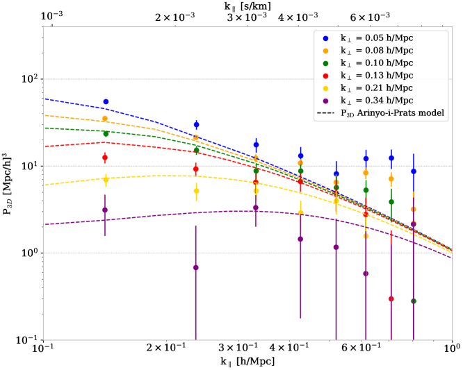
Figure 9: Average $P_{\rm{3}D}$ measurement from SDSS DR16 data at $z\simeq 2.3$, derived from the $P_{\times}$ measurements at $z=2.2$ and $z=2.4$. We converted all units to $h^{-1}$Mpc, using the formulae in 2.4 and the reference cosmology given in 3.1. For illustration, dashed lines represent the $P_{\rm{3}D}$ model of Eqn. 3.1, setting $\beta$ = 1.735 and all other parameters as given in Tables 2 and 3 of [60] (Fiducial simulation, $z=2.4$).

For an illustrative purpose only, we also represent the $P_{\rm{3}D}$ model curves from Eqn. 3.1, with parameters matching those of [60] (Tables 2 and 3, Fiducial simulation) at $z=2.4$, with the exception of the $\beta$ parameter, which we set to 1.735. The reasonably close alignment between these curves and the data points shows that our measurement provides physically sound results.

Correlated sky-subtraction noise

A detailed study of systematic effects on these $P_{\times}$ and $P_{\rm{3}D}$ measurements goes beyond the scope of this article. Statistical fluctuations are certainly the main limiting factor of the measurement at this stage. We expect several of the known systematic effects impacting $P_{\rm{1}D}$ to have a similar effect on $P_{\times}$.

On the other hand, let us focus here on an effect which was not impacting previous $P_{\rm{1}D}$ measurements: the correlated noise between two spectra contributing to a given line-of-sight pair $(i,j)$. As mentioned in Section 2.3, to compute $P_{\times}$, we assumed $\langle\tilde{\delta}_{i,n}\tilde{\delta}_{j,n}^{*}\rangle=0$ for $i\neq j$. In the case of SDSS Ly$\alpha$ data, noise correlations between nearby lines-of-sight were studied in details in [82, 48]. Most of the correlations come from the sky subtraction procedure: all the spectra from a given exposure, located on the same half-plate (spectrograph), are sky-subtracted with a common sky model. This sky model is obtained from a limited sample of sky spectra, whose fluctuations are therefore imprinted on all quasar spectra from the same half-plate. Given the SDSS survey strategy, a large fraction of nearby quasars were observed in the same exposure. This results in artificial correlations in the $\delta$ field for small transverse separations. In [48], this was measured on DR16 data and parameterized using the following equation:

$$\xi_{\rm 3D,sky}(r_{\parallel},r_{\perp})=\frac{A_{\rm sky}}{\sigma_{\rm sky}\sqrt{2\pi}}\exp\left(-\frac{r_{\perp}^{2}}{2\sigma_{\rm sky}^{2}}\right)\quad\quad{\rm for}\;r_{\parallel}=0,\quad{\rm else}\;0$$ (4.3)

The parameters are $A_{\rm sky}=9\times 10^{-3}$, $\sigma_{\rm sky}=31\,h^{-1}$ Mpc, according to the result of a full fit of $\xi_{\rm 3D}$ in the Ly$\alpha$ forest. Also, this expression is for a binned measurement of $\xi_{\rm 3D}$: the longitudinal binning $\Delta r_{\parallel}=4\,h^{-1}$ Mpc corresponds to a velocity bin $\Delta v=H(z)\,\Delta r_{\parallel}$. From this expression for $\xi_{\rm 3D,sky}$, we therefore derive:

$$P_{\times,{\rm sky}}(r_{\perp},k_{\parallel})=\frac{\sqrt{2\pi}\Delta v\,A_{\rm sky}}{\sigma_{\rm sky}}\exp\left(-\frac{r_{\perp}^{2}}{2\sigma_{\rm sky}^{2}}\right)$$ (4.4)

This is an additive contribution, independent of $k_{\parallel}$. It has the same angular dependence as $\xi_{\rm 3D,sky}$, which is relatively small in our case since $\sigma_{\rm sky}\sim 0.5^{\circ}$, and we consider angular separations much smaller than this value. The order of magnitude is $P_{\times,{\rm sky}}\sim 1$ km/s. This is a non-negligible contribution, especially for large $k_{\parallel}$, which should be considered in future measurements. In our case, it remains subdominant with respect to statistical errors. As a cross-check, we performed a data-split test: the angular pair sample was split into same half-plate, and different half-plate pairs. We found no significant difference between the $P_{\times}$ measurements from both sub-samples. This confirms that this measurement is not strongly contaminated by correlated sky-subtraction noise.

5 Conclusion and outlook

In this article, we described the implementation of a new approach to measure the small-scale 3D power spectrum of the Ly$\alpha$ forest, $P_{\rm{3}D}$. The method relies on using the cross-power spectrum $P_{\times}(\theta,k_{\parallel})$, which can be estimated by correlating 1D Fourier transforms, $\tilde{\delta}_{i}(k_{\parallel})$, of individual line-of-sight samples according to Eqn. 2.9. This is a straightforward extension of the 1D FFT method widely used to estimate $P_{\rm{1}D}$. Its simplicity, both conceptually and in terms of numerical execution, is its key advantage. Compared to the quadratic estimator approach implemented in [62], our method demands significantly less computational time.

We validated our pipeline using simulated samples of Ly$\alpha$ forests, created from a hydrodynamical simulation box of size 150 $h^{-1}$Mpc at z = 2.0. Although the cosmological volume covered by this simulation sample is small with respect to the SDSS or DESI surveys footprints, it is good enough to measure $P_{\rm{3}D}$ at the “small” scales considered here. To strengthen our proof-of-principle, we also applied our method to the eBOSS DR16 Ly$\alpha$ forest data, for two redshift bins centered at $z=2.2$ and $z=2.4$. Unlike the case of $P_{\rm{1}D}$, the small number of nearby line-of-sight pairs in the data sets, results in very large statistical error bars. Still, we were able to measure for the first time $P_{\times}$ and $P_{\rm{3}D}$ for $(k_{\parallel},k_{\perp})$ values in the $\sim 0.1-1\,h~{}{\rm Mpc^{-1}}$ range. Our measurement fairly compares with analytical formulae derived from simulations.

The statistical limitation of this measurement contrasts with the case of $P_{\rm{1}D}$. Large Ly$\alpha$ forest samples from upcoming spectroscopic surveys, like DESI [83] and WEAVE [84] will offer good opportunities to measure $P_{\times}$ and $P_{\rm{3}D}$: with respect to SDSS, the line-of-sight density of these surveys is expected to increase by a factor of $\sim 4$, so that the pair statistics at small separation angles will be larger by more than an order of magnitude. This will lead to a substantial decrease of the statistical uncertainties.

Clearly, the impact of systematic effects on those measurements should be carefully assessed in future work. However, we expect that these effects will be similar to those affecting $P_{\rm{1}D}$ measurements. In some cases, their intensity should naively be smaller than in the case of $P_{\rm{1}D}$. For example, the effect of uncorrelated noise is essentially cancelled out when cross-correlating different lines-of-sight. Also, continuum fitting mostly generates correlations between $\delta$ pixel values along an individual line-of-sight [63]. The same should hold for high-column density systems [85]. One exception is the impact of correlated noise, since nearby quasars are often observed during the same exposure with large multi-object spectrographs. In this article we presented an order-of-magnitude estimation of this effect in the case of SDSS data.

The physical interpretation of $P_{\times}$ and $P_{\rm{3}D}$ measurements is left for future work. There are several possible approaches to fitting these data to models tightly connected to the way $P_{\rm{3}D}$ is inferred from $P_{\times}$:

• The most straightforward approach will involve directly fitting $P_{\times}$ using a full modelling, which is essentially a simple extension of that used for $P_{\rm{1}D}$ alone. This is the most natural strategy since $P_{\times}$ is our primary observable. In particular, the impact of observational systematic effects will be best understood in separate $(\theta,k_{\parallel})$ bins. Additionally, computing $P_{\times}$ from hydrodynamical simulation outputs is as easy as computing $P_{\rm{1}D}$ or $P_{\rm{3}D}$. This approach is also best suited to understand the differences between contributions of $P_{\rm{1}D}$ alone and contributions of transverse correlations, to physical constraints on IGM and cosmological parameters.

• It will also be possible to infer $P_{\rm{3}D}$ from $P_{\times}$ using a full likelihood, or quadratic estimator inference, identically to what was pioneered in [62].

• Finally, using either $P_{\times}$ or $P_{\rm{3}D}$, it should be possible to fit analytic formulae that connect $P_{\rm{3}D}$ to the linear matter power spectrum such as proposed in [57, 60, 61]. Correlations between fit parameters should be reduced with respect to the case of $P_{\rm{1}D}$ alone, thanks to the $(k_{\parallel},k_{\perp})$ dependence of $P_{\rm{3}D}$. This should provide a fast, but hopefully reasonably accurate way to infer the properties of the linear power spectrum without resorting to a full simulation-based approach.

The interpretation of $P_{\times}$ or $P_{\rm{3}D}$ measurements is expected to disentangle various physical effects that are at play in the Ly$\alpha$ forest, and that are too degenerate to be robustly separated using $P_{\rm{1}D}$ alone [64]. This is in particular the case of degeneracies between a possible primordial cut-off in the power spectrum, associated for example to a Warm Dark Matter scenario, and thermal properties of the IGM [86]. We anticipate that, using our method, precise measurements of $P_{\times}$ and $P_{\rm{3}D}$ are within reach with the upcoming spectroscopic data from DESI and WEAVE.

References

- [1] J.E. Gunn and B.A. Peterson, On the Density of Neutral Hydrogen in Intergalactic Space., Astrophy. J. 142 (1965) 1633.
- [2] A.A. Meiksin, The Physics of the Intergalactic Medium, Rev. Mod. Phys. 81 (2009) 1405 [0711.3358].
- [3] BOSS collaboration, The clustering of galaxies in the completed SDSS-III Baryon Oscillation Spectroscopic Survey: cosmological analysis of the DR12 galaxy sample, Mon. Not. Roy. Astron. Soc. 470 (2017) 2617 [1607.03155].
- [4] N. Katz, D.H. Weinberg and L. Hernquist, Cosmological simulations with TreeSPH, Astrophys. J. Suppl. 105 (1996) 19 [astro-ph/9509107].
- [5] Z. Lukić, C.W. Stark, P. Nugent, M. White, A.A. Meiksin and A. Almgren, The Lyman forest in optically thin hydrodynamical simulations, MNRAS 446 (2015) 3697 [1406.6361].
- [6] R.A.C. Croft, D.H. Weinberg, N. Katz and L. Hernquist, Recovery of the power spectrum of mass fluctuations from observations of the Lyman alpha forest, Astrophys. J. 495 (1998) 44 [astro-ph/9708018].
- [7] P. McDonald, J. Miralda-Escude, M. Rauch, W.L.W. Sargent, T.A. Barlow, R. Cen et al., The Observed probability distribution function, power spectrum, and correlation function of the transmitted flux in the Lyman-alpha forest, Astrophys. J. 543 (2000) 1 [astro-ph/9911196].
- [8] R.A.C. Croft, D.H. Weinberg, M. Pettini, L. Hernquist and N. Katz, The Power spectrum of mass fluctuations measured from the Lyman alpha forest at redshift Z = 2.5, Astrophys. J. 520 (1999) 1 [astro-ph/9809401].
- [9] T.S. Kim, M. Viel, M.G. Haehnelt, R.F. Carswell and S. Cristiani, The power spectrum of the flux distribution in the lyman-alpha forest of a large sample of uves qso absorption spectra (luqas), Mon. Not. Roy. Astron. Soc. 347 (2004) 355 [astro-ph/0308103].
- [10] M. Walther, J.F. Hennawi, H. Hiss, J. Oñorbe, K.-G. Lee, A. Rorai et al., A New Precision Measurement of the Small-scale Line-of-sight Power Spectrum of the Ly Forest, Astrophys. J. 852 (2018) 22 [1709.07354].
- [11] C. Yèche, N. Palanque-Delabrouille, J. Baur and H. du Mas des Bourboux, Constraints on neutrino masses from Lyman-alpha forest power spectrum with BOSS and XQ-100, JCAP 06 (2017) 047 [1702.03314].
- [12] V. Iršič et al., The Lyman forest power spectrum from the XQ-100 Legacy Survey, Mon. Not. Roy. Astron. Soc. 466 (2017) 4332 [1702.01761].
- [13] A. Day, D. Tytler and B. Kambalur, Power spectrum of the flux in the Lyman-alpha forest from high-resolution spectra of 87 QSOs, Mon. Not. Roy. Astron. Soc. 489 (2019) 2536.
- [14] N.G. Karaçaylı et al., Optimal 1D Ly forest power spectrum estimation – II. KODIAQ, SQUAD, and XQ-100, Mon. Not. Roy. Astron. Soc. 509 (2022) 2842 [2108.10870].
- [15] SDSS collaboration, The Lyman-alpha forest power spectrum from the Sloan Digital Sky Survey, Astrophys. J. Suppl. 163 (2006) 80 [astro-ph/0405013].
- [16] N. Palanque-Delabrouille et al., The one-dimensional Ly-alpha forest power spectrum from BOSS, Astron. Astrophys. 559 (2013) A85 [1306.5896].
- [17] S. Chabanier et al., The one-dimensional power spectrum from the SDSS DR14 Ly forests, JCAP 07 (2019) 017 [1812.03554].
- [18] N.G. Karaçaylı et al., Optimal 1D Ly Forest Power Spectrum Estimation – III. DESI early data, 2306.06316.
- [19] DESI collaboration, The Dark Energy Spectroscopic Instrument: One-dimensional power spectrum from first Lyman- forest samples with Fast Fourier Transform, 2306.06311.
- [20] L. Hernquist, N. Katz, D.H. Weinberg and J. Miralda-Escude, The Lyman alpha forest in the cold dark matter model, Astrophys. J. Lett. 457 (1996) L51 [astro-ph/9509105].
- [21] L. Hui and N.Y. Gnedin, Equation of state of the photoionized intergalactic medium, Mon. Not. Roy. Astron. Soc. 292 (1997) 27 [astro-ph/9612232].
- [22] N.Y. Gnedin and L. Hui, Probing the universe with the Lyman alpha forest: 1. Hydrodynamics of the low density IGM, Mon. Not. Roy. Astron. Soc. 296 (1998) 44 [astro-ph/9706219].
- [23] P. McDonald, U. Seljak, R. Cen, P. Bode and J.P. Ostriker, Physical effects on the Ly-alpha forest flux power spectrum: Damping wings, ionizing radiation fluctuations, and galactic winds, Mon. Not. Roy. Astron. Soc. 360 (2005) 1471 [astro-ph/0407378].
- [24] S. Chabanier, F. Bournaud, Y. Dubois, N. Palanque-Delabrouille, C. Yèche, E. Armengaud et al., The impact of AGN feedback on the 1D power spectra from the Ly forest using the Horizon-AGN suite of simulations, Mon. Not. Roy. Astron. Soc. 495 (2020) 1825 [2002.02822].
- [25] M. McQuinn, The Evolution of the Intergalactic Medium, Ann. Rev. Astron. Astrophys. 54 (2016) 313 [1512.00086].
- [26] M. Walther, J. Oñorbe, J.F. Hennawi and Z. Lukić, New Constraints on IGM Thermal Evolution from the Ly Forest Power Spectrum, Astrophys. J. 872 (2019) 13 [1808.04367].
- [27] SDSS collaboration, The Linear theory power spectrum from the Lyman-alpha forest in the Sloan Digital Sky Survey, Astrophys. J. 635 (2005) 761 [astro-ph/0407377].
- [28] SDSS collaboration, Cosmological parameter analysis including SDSS Ly-alpha forest and galaxy bias: Constraints on the primordial spectrum of fluctuations, neutrino mass, and dark energy, Phys. Rev. D 71 (2005) 103515 [astro-ph/0407372].
- [29] M. Viel, M.G. Haehnelt and V. Springel, Inferring the dark matter power spectrum from the Lyman-alpha forest in high-resolution QSO absorption spectra, Mon. Not. Roy. Astron. Soc. 354 (2004) 684 [astro-ph/0404600].
- [30] C. Pedersen, A. Font-Ribera and N.Y. Gnedin, Compressing the Cosmological Information in One-dimensional Correlations of the Ly Forest, Astrophys. J. 944 (2023) 223 [2209.09895].
- [31] M. Viel, M.G. Haehnelt and V. Springel, The effect of neutrinos on the matter distribution as probed by the Intergalactic Medium, JCAP 06 (2010) 015 [1003.2422].
- [32] N. Palanque-Delabrouille et al., Neutrino masses and cosmology with Lyman-alpha forest power spectrum, JCAP 11 (2015) 011 [1506.05976].
- [33] N. Palanque-Delabrouille, C. Yèche, N. Schöneberg, J. Lesgourgues, M. Walther, S. Chabanier et al., Hints, neutrino bounds and WDM constraints from SDSS DR14 Lyman- and Planck full-survey data, JCAP 04 (2020) 038 [1911.09073].
- [34] M. Viel, G.D. Becker, J.S. Bolton and M.G. Haehnelt, Warm dark matter as a solution to the small scale crisis: New constraints from high redshift Lyman- forest data, Phys. Rev. D 88 (2013) 043502 [1306.2314].
- [35] V. Iršič et al., New Constraints on the free-streaming of warm dark matter from intermediate and small scale Lyman- forest data, Phys. Rev. D 96 (2017) 023522 [1702.01764].
- [36] J. Baur, N. Palanque-Delabrouille, C. Yeche, A. Boyarsky, O. Ruchayskiy, E. Armengaud et al., Constraints from Ly- forests on non-thermal dark matter including resonantly-produced sterile neutrinos, JCAP 12 (2017) 013 [1706.03118].
- [37] E. Armengaud, N. Palanque-Delabrouille, C. Yèche, D.J.E. Marsh and J. Baur, Constraining the mass of light bosonic dark matter using SDSS Lyman- forest, Mon. Not. Roy. Astron. Soc. 471 (2017) 4606 [1703.09126].
- [38] V. Iršič, M. Viel, M.G. Haehnelt, J.S. Bolton and G.D. Becker, First constraints on fuzzy dark matter from Lyman- forest data and hydrodynamical simulations, Phys. Rev. Lett. 119 (2017) 031302 [1703.04683].
- [39] R. Murgia, G. Scelfo, M. Viel and A. Raccanelli, Lyman- Forest Constraints on Primordial Black Holes as Dark Matter, Phys. Rev. Lett. 123 (2019) 071102 [1903.10509].
- [40] K.K. Rogers, C. Dvorkin and H.V. Peiris, Limits on the Light Dark Matter–Proton Cross Section from Cosmic Large-Scale Structure, Phys. Rev. Lett. 128 (2022) 171301 [2111.10386].
- [41] D.C. Hooper and M. Lucca, Hints of dark matter-neutrino interactions in Lyman- data, Phys. Rev. D 105 (2022) 103504 [2110.04024].
- [42] P. McDonald and J. Miralda-Escude, Measuring the cosmological geometry from the lyman alpha forest along parallel lines of sight, Astrophys. J. 518 (1999) 24 [astro-ph/9807137].
- [43] L. Hui, A. Stebbins and S. Burles, A Geometrical Test of the Cosmological Energy Contents Using the Lyman-alpha Forest, Astrophys. J. Lett. 511 (1999) L5 [astro-ph/9807190].
- [44] BOSS collaboration, The Baryon Oscillation Spectroscopic Survey of SDSS-III, Astron. J. 145 (2013) 10 [1208.0022].
- [45] A. Slosar, A. Font-Ribera, M.M. Pieri, J. Rich, J.-M. Le Goff, É. Aubourg et al., The Lyman- forest in three dimensions: measurements of large scale flux correlations from BOSS 1st-year data, JCAP 2011 (2011) 001 [1104.5244].
- [46] N.G. Busca, T. Delubac, J. Rich, S. Bailey, A. Font-Ribera, D. Kirkby et al., Baryon acoustic oscillations in the Ly forest of BOSS quasars, A&A 552 (2013) A96 [1211.2616].
- [47] BOSS collaboration, Baryon acoustic oscillations in the Ly forest of BOSS DR11 quasars, Astron. Astrophys. 574 (2015) A59 [1404.1801].
- [48] H. du Mas des Bourboux et al., The Completed SDSS-IV Extended Baryon Oscillation Spectroscopic Survey: Baryon Acoustic Oscillations with Ly Forests, Astrophys. J. 901 (2020) 153 [2007.08995].
- [49] F. Gerardi, A. Cuceu, A. Font-Ribera, B. Joachimi and P. Lemos, Direct cosmological inference from three-dimensional correlations of the Lyman forest, Mon. Not. Roy. Astron. Soc. 518 (2022) 2567 [2209.11263].
- [50] A. Cuceu, A. Font-Ribera, P. Martini, B. Joachimi, S. Nadathur, J. Rich et al., The Alcock–Paczyński effect from Lyman- forest correlations: analysis validation with synthetic data, Mon. Not. Roy. Astron. Soc. 523 (2023) 3773 [2209.12931].
- [51] A. Cuceu, A. Font-Ribera, S. Nadathur, B. Joachimi and P. Martini, Constraints on the Cosmic Expansion Rate at Redshift 2.3 from the Lyman- Forest, Phys. Rev. Lett. 130 (2023) 191003 [2209.13942].
- [52] C. Ravoux et al., A tomographic map of the large-scale matter distribution using the eBOSS—Stripe 82 Ly forest, JCAP 07 (2020) 010 [2004.01448].
- [53] DESI collaboration, Validation of the Scientific Program for the Dark Energy Spectroscopic Instrument, 2306.06307.
- [54] E. Rollinde, P. Petitjean, C. Pichon, S. Colombi, B. Aracil, V. D’Odorico et al., The Correlation of the Lyman - alpha forest in close pairs and groups of high-redshift quasars: Clustering of matter on scales 1-5 Mpc, Mon. Not. Roy. Astron. Soc. 341 (2003) 1279 [astro-ph/0302145].
- [55] G.D. Becker, W.L.W. Sargent and M. Rauch, Large-scale correlations in the Lyman-alpha forest at z=3-4, Astrophys. J. 613 (2004) 61 [astro-ph/0405205].
- [56] A. Rorai, J.F. Hennawi, J. Oñorbe, M. White, J.X. Prochaska, G. Kulkarni et al., Measurement of the small-scale structure of the intergalactic medium using close quasar pairs, Science 356 (2017) 418 [1704.08366].
- [57] P. McDonald, Toward a measurement of the cosmological geometry at Z 2: predicting lyman-alpha forest correlation in three dimensions, and the potential of future data sets, Astrophys. J. 585 (2003) 34 [astro-ph/0108064].
- [58] J.J. Givans, A. Font-Ribera, A. Slosar, L. Seeyave, C. Pedersen, K.K. Rogers et al., Non-linearities in the Lyman- forest and in its cross-correlation with dark matter halos, JCAP 09 (2022) 070 [2205.00962].
- [59] S. Chabanier, J.D. Emberson, Z. Lukić, J. Pulido, S. Habib, E. Rangel et al., Modelling the Lyman- forest with Eulerian and SPH hydrodynamical methods, Mon. Not. Roy. Astron. Soc. 518 (2022) 3754 [2207.05023].
- [60] A. Arinyo-i Prats, J. Miralda-Escudé, M. Viel and R. Cen, The Non-Linear Power Spectrum of the Lyman Alpha Forest, JCAP 12 (2015) 017 [1506.04519].
- [61] M. Garny, T. Konstandin, L. Sagunski and M. Viel, Neutrino mass bounds from confronting an effective model with BOSS Lyman- data, JCAP 03 (2021) 049 [2011.03050].
- [62] A. Font-Ribera, P. McDonald and A. Slosar, How to estimate the 3D power spectrum of the Lyman- forest, JCAP 01 (2018) 003 [1710.11036].
- [63] M. Viel, S. Matarrese, H.J. Mo, M.G. Haehnelt and T. Theuns, Probing the intergalactic medium with the lyman alpha forest along multiple lines of sight to distant qsos, Mon. Not. Roy. Astron. Soc. 329 (2002) 848 [astro-ph/0105233].
- [64] A. Rorai, J.F. Hennawi and M. White, A New Method to Directly Measure the Jeans Scale of the Intergalactic Medium Using Close Quasar Pairs, Astrophys. J. 775 (2013) 81 [1305.0210].
- [65] J.E. Bautista et al., Mock Quasar-Lyman- forest data-sets for the SDSS-III Baryon Oscillation Spectroscopic Survey, JCAP 05 (2015) 060 [1412.0658].
- [66] J. Farr et al., LyaCoLoRe: synthetic datasets for current and future Lyman- forest BAO surveys, JCAP 03 (2020) 068 [1912.02763].
- [67] A. Almgren, J. Bell, M. Lijewski, Z. Lukic and E. Van Andel, Nyx: A Massively Parallel AMR Code for Computational Cosmology, Astrophys. J. 765 (2013) 39 [1301.4498].
- [68] J. Sexton, Z. Lukic, A. Almgren, C. Daley, B. Friesen, A. Myers et al., Nyx: A Massively Parallel AMR Code for Computational Cosmology, J. Open Source Softw. 6 (2021) 3068.
- [69] M. Walther, E. Armengaud, C. Ravoux, N. Palanque-Delabrouille, C. Yèche and Z. Lukić, Simulating intergalactic gas for DESI-like small scale Lyman forest observations, JCAP 04 (2021) 059 [2012.04008].
- [70] B. Friesen, A. Almgren, Z. Lukić, G. Weber, D. Morozov, V. Beckner et al., In situ and in-transit analysis of cosmological simulations, Computational Astrophysics and Cosmology 3 (2016) 4.
- [71] S. Chabanier, C. Ravoux, E. Armengaud, Z. Lukić and J. Sexton, The accel2 project: studying the accelerated expansion of the universe by means of extremely large-volume hydrodynamical simulations of the lyman- forest, in prep.
- [72] Planck collaboration, Planck 2015 results. XIII. Cosmological parameters, Astron. Astrophys. 594 (2016) A13 [1502.01589].
- [73] J. Oñorbe, J.F. Hennawi and Z. Lukić, Self-Consistent Modeling of Reionization in Cosmological Hydrodynamical Simulations, Astrophys. J. 837 (2017) 106 [1607.04218].
- [74] D. Blas, J. Lesgourgues and T. Tram, The Cosmic Linear Anisotropy Solving System (CLASS) II: Approximation schemes, JCAP 07 (2011) 034 [1104.2933].
- [75] SDSS collaboration, The 2.5 m Telescope of the Sloan Digital Sky Survey, Astron. J. 131 (2006) 2332 [astro-ph/0602326].
- [76] S. Smee et al., The Multi-Object, Fiber-Fed Spectrographs for SDSS and the Baryon Oscillation Spectroscopic Survey, Astron. J. 146 (2013) 32 [1208.2233].
- [77] SDSS collaboration, SDSS-III: Massive Spectroscopic Surveys of the Distant Universe, the Milky Way Galaxy, and Extra-Solar Planetary Systems, Astron. J. 142 (2011) 72 [1101.1529].
- [78] SDSS collaboration, Sloan Digital Sky Survey IV: Mapping the Milky Way, Nearby Galaxies and the Distant Universe, Astron. J. 154 (2017) 28 [1703.00052].
- [79] K.S. Dawson et al., The SDSS-IV extended Baryon Oscillation Spectroscopic Survey: Overview and Early Data, Astron. J. 151 (2016) 44 [1508.04473].
- [80] B.W. Lyke et al., The Sloan Digital Sky Survey Quasar Catalog: Sixteenth Data Release, Astrophys. J. Suppl. 250 (2020) 8 [2007.09001].
- [81] SDSS-IV collaboration, The 16th Data Release of the Sloan Digital Sky Surveys: First Release from the APOGEE-2 Southern Survey and Full Release of eBOSS Spectra, Astrophys. J. Suppl. 249 (2020) 3 [1912.02905].
- [82] J.E. Bautista et al., Measurement of baryon acoustic oscillation correlations at with SDSS DR12 Ly-Forests, Astron. Astrophys. 603 (2017) A12 [1702.00176].
- [83] DESI collaboration, The DESI Experiment Part I: Science,Targeting, and Survey Design, 1611.00036.
- [84] WEAVE collaboration, WEAVE-QSO: A Massive Intergalactic Medium Survey for the William Herschel Telescope, 1611.09388.
- [85] K.K. Rogers, S. Bird, H.V. Peiris, A. Pontzen, A. Font-Ribera and B. Leistedt, Correlations in the three-dimensional Lyman-alpha forest contaminated by high column density absorbers, Mon. Not. Roy. Astron. Soc. 476 (2018) 3716 [1711.06275].
- [86] A. Garzilli, A. Boyarsky and O. Ruchayskiy, Cutoff in the Lyman forest power spectrum: warm IGM or warm dark matter?, Phys. Lett. B 773 (2017) 258 [1510.07006].