${\rm EHI}$: End-to-end Learning of Hierarchical
Index for Efficient Dense Retrieval

Abstract

Dense embedding-based retrieval is now the industry standard for semantic search and ranking problems, like obtaining relevant web documents for a given query. Such techniques use a two-stage process: (a) contrastive learning to train a dual encoder to embed both the query and documents and (b) approximate nearest neighbor search (ANNS) for finding similar documents for a given query. These two stages are disjoint; the learned embeddings might be ill-suited for the ANNS method and vice-versa, leading to suboptimal performance. In this work, we propose End-to-end Hierarchical Indexing – ${\rm EHI}$– that jointly learns both the embeddings and the ANNS structure to optimize retrieval performance. ${\rm EHI}$  uses a standard dual encoder model for embedding queries and documents while learning an inverted file index (IVF) style tree structure for efficient ANNS. To ensure stable and efficient learning of discrete tree-based ANNS structure, ${\rm EHI}$  introduces the notion of dense path embedding that captures the position of a query/document in the tree. We demonstrate the effectiveness of ${\rm EHI}$ on several benchmarks, including de-facto industry standard MS MARCO (Dev set and TREC DL19) datasets. For example, with the same compute budget, ${\rm EHI}$  outperforms state-of-the-art (SOTA) in by $0.6\%$ (MRR@10) on MS MARCO dev set and by $4.2\%$ (nDCG@10) on TREC DL19 benchmarks.

1 Introduction

Semantic search (Johnson et al., 2019) aims to retrieve relevant or semantically similar documents/items for a given query. In the past few years, semantic search has been applied to numerous real-world applications like web search, product search, and news search  (Nayak, 2019; Dahiya et al., 2021). The problem in the simplest form can be abstracted as: for a given query $q$, retrieve the relevant document(s) $d(q)$ from a static set of documents $\{d_{1},d_{2},\dots,d_{N}\}$ s.t. $d(q)=\arg\max_{1\leq j\leq N}\texttt{SIM}(\mathbf{q},\mathbf{d_{j}})$. Here SIM is a similarity function that has high fidelity to the training data $\mathcal{B}=\{(q_{i},d_{j},y_{ij})\}$. Tuple $(q_{i},d_{j},y_{ij})$ indicates if document $d_{j}$ is relevant ($y_{ij}=1$) or irrelevant ($y_{ij}=-1$) for a given query $q_{i}\in\mathcal{Q}$.

Dense embedding-based retrieval (Johnson et al., 2019; Jayaram Subramanya et al., 2019; Guo et al., 2020) is the state-of-the-art (SOTA) approach for semantic search and typically follows a two-stage process. In the first stage, it embeds the documents and the query using a deep network like BERT (Devlin et al., 2018). That is, it defines similarity $\texttt{SIM}(q,d):=\langle\mathcal{E}_{\theta}(q),\mathcal{E}_{\theta}(d)\rangle$ as the inner product between embeddings $\mathcal{E}_{\theta}(q)$ and $\mathcal{E}_{\theta}(d)$ of the query $q$ and the document $d$, respectively. $\mathcal{E}_{\theta}(\cdot)$ is a dense embedding function learned using contrastive losses (Ni et al., 2021; Menon et al., 2022).

In the second stage, approximate nearest neighbor search (ANNS) retrieves relevant documents for a given query. That is, all the documents are indexed offline and are then retrieved online for the input query. ANNS in itself has been extensively studied for decades with techniques like ScaNN (Guo et al., 2020), IVF (Sivic & Zisserman, 2003), HNSW (Malkov & Yashunin, 2020), DiskANN (Jayaram Subramanya et al., 2019) and many others being used heavily in practice.

The starting hypothesis of this paper is that the two-stage dense retrieval approach – disjoint training of the encoder and ANNS – is sub-optimal due to the following reasons:

Misalignment of representations: When the encoder and ANNS are trained separately, there is no explicit optimization objective that ensures that the representations learned by the encoder are aligned with the requirements of the ANNS technique. For example, the documents might be clustered in six clusters to optimize encoder loss. However, due to computational constraints, ANNS might allow only five branches/clusters, thus splitting or merging clusters unnaturally and inaccurately.

Ignoring query distribution: Generic ANNS techniques optimize for overall retrieval efficiency without considering the query distribution. As a result, the indexing structure might not be optimal for a particular train/test query distribution (Jaiswal et al., 2022). See Appendix B for more details.

Motivated by the aforementioned issues, we propose ${\rm EHI}$– End-to-end learning of Hierarchical Index – that jointly trains both the encoder and the search data structure; see Figure 1. To the best of our knowledge, ${\rm EHI}$ is the first end-to-end learning method for dense retrieval. Recent methods like DSI (Tay et al., 2022) and NCI (Wang et al., 2022) do not follow a dense embedding approach and directly generate document ID, but they also require a separate hierarchical clustering/tokenization phase on embeddings from a pre-trained encoder; see Section 2 for a more detailed comparison.

${\rm EHI}$ parameterizes the hierarchical tree-based indexer with classifiers in its nodes. One key idea in ${\rm EHI}$ is to map the path taken by a query or a document in the tree with a compressed, continuous, and dense path embedding. Standard path embedding in a tree is exponentially sized in tree height, but ${\rm EHI}$’s path embeddings are linear in branching factor and tree height. ${\rm EHI}$ further uses these embeddings with contrastive loss function over (query, doc) tuples along with two other loss terms promoting diversity in indexing.

We conduct an extensive empirical evaluation of our method against SOTA techniques on standard benchmarks. For example, on FIQA dataset (Maia et al., 2018) – a question-answering dataset – we observe that our method is $5.5\%$ more accurate than standard dense retrieval with ScaNN ANNS index (Guo et al., 2020) when restricted to visit/search only 20% of documents in the corpus. Furthermore, for FIQA, EHI shows an improvement of $5.61\%$ than the dense retrieval baselines with exact search, thus demonstrating better embedding learning as well. We attribute these improved embeddings to the fact that ${\rm EHI}$ enables integrated hard negative mining as it can retrieve irrelevant or negative documents from indexed leaf nodes of a query. Here, the indexer parameters are always fresh, unlike techniques akin to ANCE (Xiong et al., 2020).

Furthermore, our experiments on the popular MS MARCO benchmark (Bajaj et al., 2016) demonstrate that ${\rm EHI}$ shows improvements of $0.6\%$ in terms of nDCG@10 compared to dense-retrieval with ScaNN baselines when only 10% of documents are searched. Similarly, EHI provides $4.2\%$ higher nDCG@$10$ than state-of-the-art (SOTA) baselines on the MS MARCO TREC DL19 (Craswell et al., 2020) benchmarks for the same compute budget. ${\rm EHI}$ also achieves SOTA exact search performance on both MRR@$10$ and nDCG@$10$ metrics with up to $80\%$ reduction in latency, indicating the effectiveness of the joint learning objective. Similarly, we outperform SOTA architectures such as NCI on NQ320$k$ by $0.5\%$ and $\sim 2\%$ on Recall@10 and Recall@100 metrics with a model one-tenth the size! (see Section 4.2).

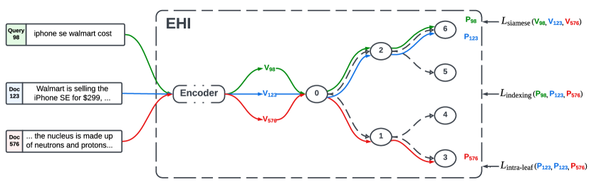
Figure 1: ${\rm EHI}$ is an end-to-end hierarchical indexer which comprises an encoder and a hierarchical tree as the indexer where the entire pipeline is learnable and differentiable. Here, variables $V_{98}$, $V_{123}$, and $V_{576}$ are dense representations (embeddings) of the text and $P_{98}$, $P_{123}$, and $P_{576}$ are path embeddings of the respective samples. To efficiently train ${\rm EHI}$ without any warm starting, we use a combination of objectives - $L_{\text{siamese}}$, $L_{\text{indexing}}$, $L_{\text{intra-leaf}}$ (see Section 3 for details).

To summarize, the paper makes the following key contributions:

• Proposed ${\rm EHI}$, the first end-to-end learning method for dense retrieval that jointly learns both the encoder and the search indexer for various downstream tasks. (see Section 3). ${\rm EHI}$ represents a paradigm shift in dense retrieval where both encoder and ANNS could be integrated and trained accurately, efficiently, and stably in a single pipeline.

• Extensive empirical evaluation of ${\rm EHI}$ on the industry standard MS MARCO benchmark and compare it to SOTA approaches like ColBERT, SGPT, cpt-text, ANCE, DyNNIBAL, etc. (see Appendix D). ${\rm EHI}$’s focus is mainly on improving retrieval accuracy for a fixed computation/search budget and is agnostic to encoder architecture, similarity computation, hard negative mining, etc.

2 Related Works

Dense retrieval (Mitra et al., 2018) underlies a myriad of web-scale applications like search (Nayak, 2019), recommendations (Eksombatchai et al., 2018; Jain et al., 2019), and is powered by (a) learned representations (Devlin et al., 2018; Kolesnikov et al., 2020; Radford et al., 2021), (b) ANNS (Johnson et al., 2019; Sivic & Zisserman, 2003; Guo et al., 2020) and (c) LLMs in retrieval (Tay et al., 2022; Wang et al., 2022; Guu et al., 2020).

Representation learning. Powerful representations are typically learned through supervised and un/self-supervised learning paradigms that use proxy tasks like masked language modeling (Devlin et al., 2018) and autoregressive training (Radford et al., 2018). Recent advances in contrastive learning (Gutmann & Hyvärinen, 2010) helped power strong dual encoder-based dense retrievers (Ni et al., 2021; Izacard et al., 2021; Nayak, 2019). They consist of query and document encoders, often shared, which are trained with contrastive learning using limited positively relevant query and document pairs (Menon et al., 2022; Xiong et al., 2020). While most modern-day systems use these learned representations as is for large-scale ANNS, there is no need for them to be aligned with the distance metrics or topology of the data structures. Recent works have tried to address these concerns by warm-starting the learning with a clustering structure (Gupta et al., 2022) but fall short of learning jointly optimized representations alongside the search structure.

Approximate nearest neighbor search (ANNS). The goal of ANNS is to retrieve almost nearest neighbors without paying exorbitant costs of retrieving true neighbors  (Clarkson, 1994; Indyk & Motwani, 1998; Weber et al., 1998). The “approximate” nature comes from pruning-based search data structures (Sivic & Zisserman, 2003; Malkov & Yashunin, 2020; Beygelzimer et al., 2006) as well as from the quantization based cheaper distance computation (Jegou et al., 2010; Ge et al., 2013). This paper focuses on ANNS data structures and notes that compression is often complementary. Search data structures reduce the number of data points visited during the search. This is often achieved through hashing (Datar et al., 2004; Salakhutdinov & Hinton, 2009; Kusupati et al., 2021), trees (Friedman et al., 1977; Sivic & Zisserman, 2003; Bernhardsson, 2018; Guo et al., 2020) and graphs (Malkov & Yashunin, 2020; Jayaram Subramanya et al., 2019). ANNS data structures also carefully handle the systems considerations involved in a deployment like load-balancing, disk I/O, main memory overhead, etc., and often tree-based data structures tend to prove highly performant owing to their simplicity and flexibility (Guo et al., 2020). For a more comprehensive review of ANNS structures, please refer to Cai (2021); Li et al. (2020); Wang et al. (2021).

Encoder-decoder for Semantic Search. Recently, there have been some efforts towards modeling retrieval as a sequence-to-sequence problem. In particular, Differential Search Index (DSI) (Tay et al., 2022) and more recent Neural Corpus indexer (NCI) (Wang et al., 2022) method proposed encoding the query and then find relevant document by running a learned decoder. However, both these techniques, at their core, use a separately computed hierarchical k-means-based clustering of document embeddings for semantically assigning the document-id. That is, they also index the documents using an ad-hoc clustering method which might not be aligned with the end objective of improving retrieval accuracy. In contrast, ${\rm EHI}$ jointly learns both representation and a k-ary tree-based search data structure end-to-end. This advantage is reflected on MS MARCO dataset ${\rm EHI}$ is upto 7.12% more accurate (in terms of nDCG@10) compared to DSI. Recently, retrieval has been used to augment LLMs also  (Guu et al., 2020; Izacard & Grave, 2020b; a; Izacard et al., 2022). We would like to stress that the goal with LLMs is language modeling while retrieval’s goal is precise document retrieval. However, retrieval techniques like ${\rm EHI}$ can be applied to improve retrieval subcomponents in such LLMs.

3 End-to-end Hieararchical Indexing (${\rm EHI}$)

Problem definition and Notation. Consider a problem with a corpus of $N$ documents $\mathcal{D}=\{d_{1},...,d_{N}\}$, a set of $Q$ training queries $\mathcal{Q}=\{q_{1},...,q_{Q}\}$, and training data $(q_{i},d_{k},y_{ik})$, where $y_{ik}\in\{-1,1\}$ is the label for a given training (query, document) tuple and $y_{ik}=1$ denotes that $d_{k}$ is relevant to $q_{i}$. Given these inputs, the goal is to learn a retriever that maps a given query to a set of relevant documents while minimizing the computation cost. While wall-clock time is the primary cost metric, comparing different methods against it is challenging due to very different setups (language, architecture, parallelism, etc.). Instead, we rely on recall vs. % searched curves, widely considered a reasonable proxy for wall-clock time modulo other setup/environment changes (Guo et al., 2020).

3.1 Overview of ${\rm EHI}$

At a high level, ${\rm EHI}$ has three key components: Encoder $\mathcal{E}_{\theta}$, Indexer $\mathcal{I}_{\phi}$ and Retriever. Parameters $\theta$ of the query/document encoder and $\phi$ of the indexer are the trainable parameters of ${\rm EHI}$. Unlike most existing techniques, which train the encoder and indexer in a two-step disjoint process, we train both the encoder and indexer parameters jointly with an appropriate loss function; see Section 3.5. Learning the indexer – generally a discontinuous function – is a combinatorial problem that also requires multiple rounds of indexing the entire corpus. However, by modeling the indexer using a hierarchical tree and its “internal representation” as compressed path embedding, we demonstrate that the training and retrieval with encoder$+$indexer can be executed efficiently and effectively.

In the following sections, we provide details of the encoder and indexer components. In Section 3.4, we detail how encoder$+$indexer can be used to retrieve specific documents for a given query, which is used both for inference and hard-negative mining during training. Section 3.5 provides an overview of the training procedure. Finally, Section 3.6 summarizes how documents are ranked after retrieval.

3.2 Encoder $\mathcal{E}_{\theta}$: Dense embedding of query/documents

Our method is agnostic to the architecture used for dual encoder. But for simplicity, we use standard dual encoder (Ni et al., 2021) to map input queries and documents to a common vector space. That is, encoder $\mathcal{E}_{\theta}$ parameterized by $\theta$, maps query ($q\in\mathcal{Q}$) and document ($d\in\mathcal{D}$) to a common vector space: $\mathcal{E}_{\theta}(q)\in\mathbb{R}^{m}\text{, and}~{}\mathcal{E}_{\theta}(d)\in\mathbb{R}^{m}$, where $m$ is the embedding size of the model (768 here). While such an encoder can also be multi-modal as well as multi-vector, for simplicity, we mainly focus on standard textual data with single embedding per query/document. We use the standard BERT architecture for encoder $\mathcal{E}_{\theta}$ and initialize parameters $\theta$ using a pre-trained Sentence-BERT distilbert model (Reimers & Gurevych, 2019). Our base model has 6 layers, 768 dimensions, 12 heads with 66 million parameters. We then fine-tune the final layer of the model for the target downstream dataset.

3.3 Indexer $\mathcal{I}_{\phi}$: Indexing of query/document in the hierarchical data structure

${\rm EHI}$’s indexer ($\mathcal{I}_{\phi}$) is a tree with height $H$ and branching factor $B$. Each tree node contains a classifier that provides a distribution over its children. So, given a query/document, we can find out the leaf nodes that the query/document indexes into, as well as the probabilistic path taken in the tree.

The final leaf nodes reached by the query are essential for retrieval. But, we also propose to use the path taken by a query/document in the tree as an embedding of the query/document – which can be used in training through the loss function. However, the path a query/document takes is an object in an exponentially large (in height $H$) vector space, owing to $B^{H}$ leaf nodes, making it computationally intractable even for a small $H$ and $B$.

Instead, below, we provide a significantly more compressed path embedding – denoted by $\mathcal{T}(\cdot;\phi)$ and parameterized by $\phi$ – embeds any given query or document in a relatively low-dimensional ($B\cdot H$) vector space. For simplicity, we denote the query and the document path embedding as $\mathcal{T}_{\phi}(q)=\mathcal{T}(\mathcal{E}_{\theta}(q);\phi)$ and $\mathcal{T}_{\phi}(d)=\mathcal{T}(\mathcal{E}_{\theta}(d);\phi)$, respectively.

We construct path embedding of a query/document as:

$$\mathcal{T}(\mathcal{E}_{\theta}(q)=\mathcal{T}(\mathcal{E}_{\theta}(q);\phi)=[\mathbf{p}^{H};\mathbf{p}^{H-1};\dots;\mathbf{p}^{1}],$$

Where $\mathbf{p}^{h}\in[0,1]^{B}$ denotes the probability distribution of children nodes for a parent at height $h$. For a given leaf $l$, say path from root node is defined as $\mathbf{l}=[i^{1}_{l},i^{2}_{l}\dots i^{H}_{l}]$ where $i^{h}_{l}\in[1\dots B]$ for $h\in[H]$. The probability at a given height in a path is approximated using a height-specific simple feed-forward neural network parameterized by $\mathbf{W}_{h+1}\in\mathbb{R}^{(B\cdot h+m)\times B}$ and $\mathbf{U}_{h+1}\in\mathbb{R}^{(B\cdot h+m)\times(B\cdot h+m)}$ ($m$ is the embedding size). That is,

$$\mathbf{p}^{h+1} =\texttt{Softmax}(\mathbf{W}_{h+1}^{\top}\mathcal{F}([\mathbf{o}(i^{h}_{l});\mathbf{o}(i^{h-1}_{l});\dots;\mathbf{o}(i^{1}_{l});\mathcal{E}_{\theta}(q)];\mathbf{U}_{h+1}))\cdot\mathbf{p}^{h}[i^{h}_{l}]$$ (1)

where one-hot-vector $\mathbf{o}(i)$ is the $i$-th canonical basis vector and $\mathcal{F}$ is a non-linear transformation given by $\mathcal{F}(\mathbf{x};\mathbf{U}_{h})=\mathbf{x}+\texttt{ReLU}(\mathbf{U}_{h}^{\top}\mathbf{x})$.

In summary, the path embedding for height 1 represents a probability distribution over the leaves. During training, we compute path embedding for higher heights for only the most probable path, ensuring that the summation of leaf node logits remains a probability distribution. Also, the indexer and path embedding function $\mathcal{T}(\cdot;\phi)$ has the following collection of trainable parameters: $\phi=\{\mathbf{W}_{H},\dots,\mathbf{W}_{1},\mathbf{U}_{H},\dots,\mathbf{U}_{1}\}$, which we learn by optimizing a loss function based on the path embeddings; see Section 3.5.

3.4 Retriever: Indexing items for retrieving

Indexing and retrieval form a backbone for any search structure. ${\rm EHI}$ efficiently encodes the index path of the query and documents in $(B\cdot H)$-dimensional embedding space. During retrieval for a query q, ${\rm EHI}$ explores the tree structure to find the “most relevant” leaves and retrieves documents associated with those leaves. For retrieval, it requires encoder and indexer parameters $(\theta,\phi)$ along with Leaf, document hashmap $\mathcal{M}$.

The relevance of a leaf $l$ for a query $q$ is measured by the probability of a query reaching a leaf at height $H$ ($\mathcal{P}(q,l,H)$). Recall from previous section that path to a leaf $l$ is defined as $\mathbf{l}=[i^{1}_{l},i^{2}_{l}\dots i^{H}_{l}]$ where $i^{h}_{l}\in[1\dots B]$ for $h\in[H]$. The probability of reaching a leaf $l$ for a given query $q\in\mathcal{Q}$ to an arbitrary leaf $l\in\texttt{Leaves}$ can be computed as $\mathcal{P}(q,l,H)=\mathbf{p}^{H}[i_{l}^{H}]$ using equation 1. But, we only need to compute the most probable leaves for every query during inference, which we obtain by using the standard beam-search procedure summarized below:

1. For all parent node at height $h-1$, compute probability of reaching their children $\hat{S}=\cup_{c\in\texttt{child}(p)}\mathcal{P}(q,c,h)~{}\forall_{p\in P}$ .

2. Keep top $\beta$ children based on score $\hat{S}$ and designate them as the parents for the next height.

Repeat steps 1 and 2 until the leaf nodes are reached.

Once we select $\beta$ leaves ${\rm EHI}$ retrieves documents associated with each leaf, which is stored in the hashmap $\mathcal{M}$. To compute this hash map, ${\rm EHI}$ indexes each document $d\in\mathcal{D}$ (similar to query) with $\beta=1$. Here, $\beta=1$ is a design choice considering memory and space requirements and is kept as a tuneable parameter. Algorithm 2 in the appendix depicts the approach used by our Indexer for better understanding.

3.5 Training ${\rm EHI}$

Given the definition of all three ${\rm EHI}$ components – encoder, indexer, and retriever – we are ready to present the training procedure. As mentioned earlier, the encoder and the indexer parameters ($\theta;\phi$) are optimized simultaneously with our proposed loss function, which is designed to have the following properties: a) Relevant documents and queries should be semantically similar, b) documents and queries should be indexed together iff they are relevant, and c) documents should be indexed together iff they are similar.

Given the encoder and the indexer, we design one loss term for each of the properties mentioned above and combine them to get the final loss function. To this end, we first define the triplet loss as:

$$L(\mathcal{E}_{\theta}(q),\mathcal{E}_{\theta}(d_{+}),\mathcal{E}_{\theta}(d_{-}))=[\mathcal{E}_{\theta}(q)^{\top}\mathcal{E}_{\theta}(d_{-})-\mathcal{E}_{\theta}(q)^{\top}\mathcal{E}_{\theta}(d_{+})+\gamma]_{+},$$ (2)

where we penalize if similarity between query $q$ and an irrelevant document $d_{-}$ ($y(q,d_{-})\neq 1$) is within $\gamma$ margin of the corresponding similarity between $q$ and a relevant document $d_{+}$ ($y(q,d_{+})=1$).We now define the following three loss terms:

1. Semantic Similarity: the first term is a standard dual-encoder contrastive loss between a relevant document $d_{+}$ – i.e., $y(q,d_{+})=+1$ – and an irrelevant document with $y(q,d_{-})\neq 1$.

   $$L_{\text{siamese}}=L(\mathcal{E}_{\theta}(q),\mathcal{E}_{\theta}(d_{+}),\mathcal{E}_{\theta}(d_{-});\theta)$$ (3)

2. Indexing Similarity: the second term is essentially a similar contrastive loss over the query, relevant-doc, irrelevant-doc triplet, but where the query and documents are represented using the path-embedding $\mathcal{T}_{\phi}(\cdot)$ given by the indexer $\mathcal{I}_{\phi}$.

   $$L_{\text{indexing}}=L(\mathcal{T}_{\phi}(q),\mathcal{T}_{\phi}(d_{+}),\mathcal{T}_{\phi}(d_{-});\theta,\phi)$$ (4)

3. Intra-leaf Similarity: to spread out irrelevant docs, third loss applies triplet loss over the sampled relevant and irrelevant documents for a query $q$. Note that we apply the loss only if the two docs are semantically dissimilar according to the latest encoder, i.e., $\texttt{SIM}(\mathbf{a},\mathbf{b})=\frac{\mathbf{a}^{T}\mathbf{b}}{|\mathbf{a}||\mathbf{b}|}<\tau$ for a pre-specified threshold $\tau=0.9$.

   $$L_{\text{intra-leaf}}=\mathbf{1}\{\texttt{SIM}(\mathcal{E}_{\theta}(d_{+}),\mathcal{E}_{\theta}(d_{-}))<\tau\}L(\mathcal{T}_{\phi}(d_{+}),\mathcal{T}_{\phi}(d_{+}),\mathcal{T}_{\phi}(d_{-});\theta,\phi)$$ (5)

The final loss function $\mathcal{L}$ is given as the weighted sum of the above three losses:

$$\mathcal{L}(q,d_{+},d_{-};\theta,\phi)=\lambda_{1}L_{\text{siamese}}+\lambda_{2}L_{\text{indexing}}+\lambda_{3}L_{\text{intra-leaf}}$$ (6)

Here $\gamma$ is set to 0.3 for all loss components, and $\lambda_{1},\lambda_{2},\lambda_{3}$ are tuneable hyper-parameters. Our trainer (see Algorithm 1) learns $\theta$ and $\phi$ by optimizing $\mathcal{L}$ using standard techniques; for our implementation we used AdamW (Loshchilov & Hutter, 2017).

Note that the loss function only uses in-batch documents’ encoder embeddings and path embeddings, i.e., we are not even required to index all the documents in the tree structure, thus allowing efficient joint training of both encoder and indexer. To ensure fast convergence, we use hard negatives mined from the indexed leaves of a given query $q$ for which we require documents to be indexed in the tree. But, this procedure can be done once in every $r$ step where $r$ is a hyper-parameter set to 5 by default across our experiments. We will like to stress that existing methods like DSI, NCI, or ANCE not only have to use stale indexing of documents, but they also use stale or even fixed indexers – like DSI, NCI learns a fixed semantic structure over docids using one-time hierarchical clustering. In contrast, ${\rm EHI}$ jointly updates the indexer and the encoder in each iteration, thus can better align the embeddings with the tree/indexer.

3.6 Re-ranking and Evaluation

This section describes the re-ranking step and the test-time evaluation process after retrieval. In Section 3.4, we discussed how each document is indexed, and we now have a learned mapping of $d\times l$, where $d$ is the corpus size, and $l$ is the number of leaves. Given a query at test time, we perform a forward pass similar to the indexing pipeline presented in Section 3.4 and find the top-$b$ leaves ($b$ here is the beam size) the given query reaches. We collate all the documents that reached these $b$ leaves (set operation to avoid any repetition of the same documents across multiple leaves) and rank them based on an appropriate similarity metric such as cosine similarity, dot product, manhattan distance, etc. We use the cosine similarity metric for ranking throughout our experiments presented in Section 4.2.

4 Experiments

In this section, we present empirical evaluation of ${\rm EHI}$ on standard dense retrieval benchmarks. The goal of empirical evaluation is twofold: (a) highlight the paradigm shift of training both encoder and ANNS in an end-to-end fashion (${\rm EHI}$) is more favorable to training them in an disjoint fashion (off-the-shelf indexers such as ScaNN, Faiss-IVF, etc.), (b) understand ${\rm EHI}$’s stability wrt various hyper-parameters and how to set them up appropriately.

We note that due to typical scale of retrieval systems, a method’s ability to retrieve relevant documents under strict latency budget is critical, and defines success of a method. So, we would want to compare query throughput against recall/MRR, but obtaining head-to-head latency numbers is challenging as different systems are implemented using different environments and optimizations. So, following standard practice in the ANNS community, we use a fraction of documents visited/searched as a proxy for latency  (Jayaram Subramanya et al., 2019; Guo et al., 2020). Appendix C provides exact training hyperparameters of ${\rm EHI}$.

4.1 Experimental Setup

Datasets:

We evaluate ${\rm EHI}$ on four standard but diverse retrieval datasets of increasing size: SciFact (Wadden et al., 2020), FIQA (Maia et al., 2018), MS MARCO (Bajaj et al., 2016) and NQ320$k$ (Kwiatkowski et al., 2019). Appendix A provides additional details about these datasets.

Baselines.

We consider five baseline methods to evaluate against ${\rm EHI}$. In particular, baselines DE+Exact-search, DE+ScaNN, and DE+Faiss-IVF are standard dense retrieval methods with dual-encoder (DE) architecture (Menon et al., 2022) trained using Siamese loss (Chopra et al., 2005). The three methods use three different ANNS methods for retrieval: Exact-search, ScaNN (Guo et al., 2020), and Faiss-IVF (Johnson et al., 2019). DSI (Tay et al., 2022) and NCI (Wang et al., 2022) are the remaining two main baselines. We report DSI numbers on MS MARCO using an implementation validated by the authors. However, we note that NCI fails to scale to large datasets like MS MARCO. For ${\rm EHI}$ and baseline dual-encoder (DE) models, we use a pre-trained Sentence-BERT (Reimers & Gurevych, 2019) fine-tuned appropriately on the downstream dataset using contrastive loss. For DE baselines, only the encoder is fine-tuned, while the ANNS structure (off-the-shelf indexers) is built on top of the learned representations.

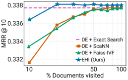
(a) MSMARCO: MRR@10

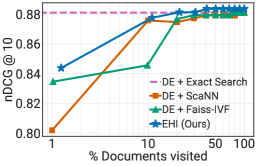
(b) TREC DL19: nDCG@10

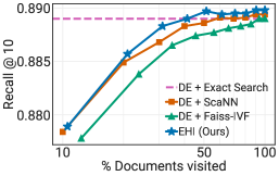
(c) NQ320$k$: R@10

Figure 2: ${\rm EHI}$ is significantly more accurate than DE + ScaNN or Faiss-IVF, especially when restricted to visit a small fraction of documents. See Figure 5 in Appendix for results on Scifact, Fiqa.

4.2 Results

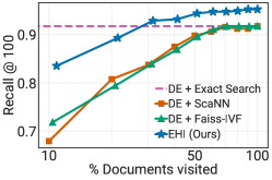
(a) SciFact: Recall@100

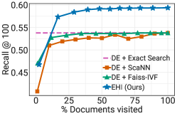
(b) FIQA: Recall@100

Figure 5: (a), (b): Recall@100 of ${\rm EHI}$ and baselines on Scifact and Fiqa dataset. ${\rm EHI}$ is significantly more accurate than dual encoder + ScaNN or Faiss-IVF baselines, especially when computationally restricted to visit a small fraction of documents. For example, on Scifact dataset, at $10$% document visit rate, ${\rm EHI}$ has $11.7$% higher Recall@100 than baselines.

SciFact. We first start with the small-scale SciFact dataset. Figure 5(a) and Table 8 compares ${\rm EHI}$ to three DE baselines. Clearly, ${\rm EHI}$’s recall-compute curve dominates that of DE+ScaNN and DE+Faiss-IVF. For example, when allowed to visit/search about 10% of documents, ${\rm EHI}$ obtains up to +15.64% higher Recall@$100$. Furthermore, ${\rm EHI}$ can outperform DE+Exact Search with a 60% reduction in latency. Finally, representations from ${\rm EHI}$’s encoder with exact search can be as much as 4% more accurate (in terms of Recall@$100$) than baseline dual-encoder+Exact Search, indicating effectiveness of ${\rm EHI}$’s integrated hard negative mining.

FIQA. Here also we observe a similar trend as SciFact; see Figure 5(b) and Table 9. That is, when restricted to visit only 15% documents (on an average), ${\rm EHI}$ outperforms ScaNN and Faiss-IVF in Recall@100 metric by 5.46% and 4.36% respectively. Furthermore, ${\rm EHI}$ outperforms the exact search in FIQA with a 84% reduction in latency or documents visited. Finally, when allowed to visit about $50\%$ of the documents, ${\rm EHI}$ is about 5% more accurate than Exact Search, which visits all the documents. Thus indicating better quality of learned embeddings.

MS MARCO. As mentioned in Section 4.1, MS MARCO is considered the gold standard benchmark for semantic retrieval. We study the MS MARCO passage retrieval task on both standard dev set, as well as TREC DL-19 set (Craswell et al., 2020). We compare against the standard Sentence-BERT model (Huggingface, 2019), fine-tuned on MS MARCO, with Exact Search (see Table 10).

For the standard dev set, ${\rm EHI}$ is able to match or surpass the accuracy of baseline Exact Search with an 80% reduction in number of documents visited. This is in stark contrast to the baseline DE+ScaNN and DE+Faiss-IVF methods, which require visiting almost double, i.e., almost $50\%$ of the documents. Furthermore, when restricted to visiting only $1\%$ of the documents, ${\rm EHI}$ obtains 0.6% higher nDCG@10 than DE+ScaNN and DE+Faiss-IVF. Note that such a gain is quite significant for the highly challenging and well-studied MS MARCO dataset. We also compare ${\rm EHI}$ against DSI on this dataset. We note that the DSI base model with 250M parameters is almost four times the size of the current ${\rm EHI}$ model. After multiple weeks of DSI training with doc2query + atomic id + base model, DSI’s MRR@$10$ value is $26\%$, which is about 6% lower than ${\rm EHI}$ with just $\mathbf{1\%}$ visited documents. Also note that despite significant efforts, we could not scale NCI code (Wang et al., 2022) on MS MARCO due to the dataset size; the NCI paper does not provide accuracy numbers on MS MARCO dataset.

For the TREC DL-19 set, ${\rm EHI}$ is able to match or surpass the nDCG@10 of baseline Exact Search with an 78% reduction in latency. Furthermore, when restricted to visiting 1% of the documents, ${\rm EHI}$ achieves 4.2% higher nDCG@10 than DE+ScaNN and DE+Faiss-IVF.

For completeness, we compare ${\rm EHI}$’s accuracy against SOTA methods for this dataset that uses a similar-sized encoder. Note that these methods often use complementary and analogous techniques to ${\rm EHI}$, such as multi-vector similarity, etc., and can be combined with ${\rm EHI}$. Nonetheless, we observe that ${\rm EHI}$ is competitive with SOTA techniques like ColBERT with a similar encoder and is significantly more accurate than traditional DE methods like ANCE, HNSW, etc. Appendix D provides a more detailed comparison of ${\rm EHI}$ encoder against other SOTA encoders on the MS MARCO dataset. Note that any of these encoders could replace the Distilbert model used in ${\rm EHI}$ and only serve to show the efficacy of the learned representations. (see Table 2)

NQ320$k$. Finally, we present evaluation on the standard NQ320$k$ (Kwiatkowski et al., 2019) benchmark, in the setting studiedy by the NCI paper (Wang et al., 2022). ${\rm EHI}$ matches or surpasses the accuracy of baseline Exact Search with a 60% reduction in latency. Furthermore, when limited to the same compute budget, ${\rm EHI}$ outperforms DE+SCANN and DE+Faiss-IVF by up to 0.4% in Recall@10.

Comparison to DSI/NCI: Note that ${\rm EHI}$ is able to significantly outperform DSI and NCI (without query generation) despite NCI utilizing a $10\times$ larger encoder! Furthermore, even with query generation, NCI is $0.5\%$ and $\sim 2\%$ less accurate than ${\rm EHI}$ on Recall@10 and Recall@100 metrics, respectively. (see Table 2)

Our observations about ${\rm EHI}$ are statistically significant as evidenced by p-value tests Appendix E.3. Additional experiments such as the number of documents per leaf, robustness to initialization, qualitative analysis on the leaves of the indexer learned by the ${\rm EHI}$ model are depicted in Appendix E.

Table 1: Performance metrics ($\%$) evaluated on the MS MARCO dev dataset. The best value for each metric is indicated in bold font. For an exhaustive comparison refer to Table 5 in appendix

Method	MRR@10	nDCG@10
BM25	16.7	22.8
HNSW	28.9	-
DyNNIBAL	33.4	-
DeepCT	24.3	29.6
DSI	26.0	32.28
ANCE	33.0	38.8
TAS-B	-	40.8
GenQ	-	40.8
ColBERT	36.0	40.1
EHI (distilbert-cos; Ours)	33.8	39.4
EHI (distilbert-dot; Ours)	37.2	43.3

Table 2: Performance metrics ($\%$) evaluated on the NQ320$k$ dataset (Kwiatkowski et al., 2019). The best value for each metric is indicated in bold font. Please refer to Table 7 for more methods.

Method	R@10	R@100
BM25	32.48	50.54
BERT + BruteForce	53.42	73.16
BM25 + DocT5Query	61.83	76.92
ANCE (MaxP)	80.38	91.31
SEAL (Large)	81.24	91.93
DyNNIBAL	75.4	86.2
DSI	70.3	-
NCI (Large)	85.27	92.49
NCI w/ qg-ft (Large)	88.45	94.53
EHI (distilbert-cos; Ours)	88.98	96.3

4.3 Ablations

In the previous section, we demonstrated the effectiveness of ${\rm EHI}$ against multiple baselines on diverse benchmarks. In this section, we report results from multiple ablation studies to better understand the behavior of ${\rm EHI}$. Additional properties such as load balancing, effect of negative mining refresh factor, and other properties of ${\rm EHI}$ are discussed in Appendix E.

Effect of branching factor. Figure 3(a) shows recall@$100$ of ${\rm EHI}$ on SciFact with varying branching factors. We consider two versions of ${\rm EHI}$, one with exact-search that is a beam-size=branching factor (B), and with beam-size $\approx 0.1$ branching factor, i.e., restricting to about 10% visited document. Interestingly, for ${\rm EHI}$ + Exact Search, the accuracy decreases with a higher branching factor, while it increases for the smaller beam-size of $0.1$. We attribute this to documents in a leaf node being very similar to each other for high branching factors (fewer points per leaf). We hypothesize that ${\rm EHI}$ is sampling highly relevant documents for hard negatives leading to a lower exact search accuracy.

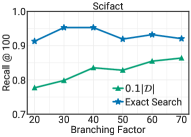
(a) Branching factor

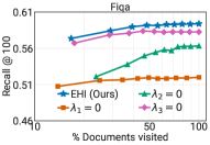
(b) Loss components

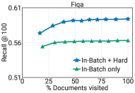
(c) Hard -ve sampling

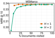
(d) Height

Figure 3: Ablation study of four major components in ${\rm EHI}$ to evaluate their contributions towards jointly learned representation and ANNS structure for state-of-the-art dense retrieval.

Ablation w.r.t loss components. Next, on FIQA dataset, we study performance of ${\rm EHI}$ when one of the loss components equation 6 is turned off; see Figure 3(b). First, we observe that ${\rm EHI}$ outperforms the other three vanilla variants, implying that each loss term contributes non-trivially to the performance of ${\rm EHI}$. Next, we observe that removing the document-similarity-based loss term ($\lambda_{3}$), Eq. equation 5, has the least effect on the performance of ${\rm EHI}$, as the other two-loss terms already capture some of its desired consequences. However, turning off the contrastive loss on either encoder embedding ($\lambda_{1}$), Eq. equation 3, or path embedding ($\lambda_{2}$), Eq. equation 4, loss leads to a significant loss in accuracy. This also indicates the importance of jointly and accurately learning both the encoder and indexer parameters.

Effect of hard negative sampling. Figure 3(c) shows recall@100 with and without hard-negative mining using the learned indexer (see Algorithm 1) on FIQA. ${\rm EHI}$ with hard negative sampling improves recall@100 significantly by $\mathbf{3.1\%}$, thus clearly demonstrating it’s importance.

Effect of height. We study the accuracy of ${\rm EHI}$ when extending to multiple heights of the tree structure to extend its effectiveness in accurately indexing extensive web-scale document collections. Traditional indexing methods that rely on a single-height approach can be computationally impractical and sub-optimal when dealing with billions or more documents. To address this challenge, ${\rm EHI}$ treats height as a hyperparameter and learns the entire tree structure end-to-end. Our experimental results in Figure 3(d) demonstrate that trees with $H=2$ also exhibit similar performance on the MS MARCO as $H=1$. This extension enhances scalability and efficiency when indexing large web-scale datasets. For instance, ${\rm EHI}$ trained on Scifact with equal number of leaves, we notice a significant speedup with increasing height; for example at $(B=64,H=1)$, $(B=8,H=2)$, and $(B=4,H=3)$, we notice a per-query latency of $2.48$ ms, $2.40$ ms, and $1.99$ ms respectively at the same computation budget. This extension to hierarchical k-ary tree is absolutely necessary for scalability and discussed in further detail in Appendix E.6.

5 Conclusions, Limitations, and Future Work

We presented ${\rm EHI}$, a framework and paradigm shift to jointly learn both the query/document encoder and the search indexer to retrieve documents efficiently. ${\rm EHI}$ is composed of three key components: encoder, indexer, and retriever; indexer generates compressed, low-dimensional path embeddings of query/documents in the tree, which is key to joint training of encoder and indexer. We demonstrated the effectiveness of ${\rm EHI}$ on a variety of standard benchmarks. Currently, path embeddings are mainly an intuitive construct without formal understanding. In the future, understanding path embeddings and providing rigorous guarantees should be of significant interest. Furthermore, combining ${\rm EHI}$ encoders that output hierarchical representations like matryoshka embeddings (Kusupati et al., 2022) or integrating with RGD (Kumar et al., 2023) to further improve generalization of tail queries should also be of interest. Finally, this paper addresses an abstract and established problem, so we don’t expect any significant additional societal implications from this work.

Appendix A Datasets

In this section, we briefly discuss the open-source datasets used in this work adapted from the Beir benchmark Thakur et al. (2021).

Scifact:

Scifact (Wadden et al., 2020) is a fact-checking benchmark that verifies scientific claims using evidence from research literature containing scientific paper abstracts. The dataset has $\sim 5000$ documents and has a standard train-test split. We use the original publicly available dev split from the task having 300 test queries and include all documents from the original dataset as our corpus. The scale of this dataset is smaller and included to demonstrate even splits and improvement over baselines even when the number of documents is in the order of 5000.

Fiqa:

Fiqa (Maia et al., 2018) is an open-domain question-answering task in the domain of financial data by crawling StackExchange posts under the Investment topic from 2009-2017 as our corpus. It consists of $57,368$ documents and publicly available test split from (Thakur et al., 2021) As the test set, we use the random sample of 500 queries provided by Thakur et al. (2021). The scale of this dataset is 10x higher than Scifact, with almost 57,638 documents in our corpus.

MS Marco:

The MSMarco benchmark Bajaj et al. (2016) has been included since it is widely recognized as the gold standard for evaluating and benchmarking large-scale information retrieval systems (Thakur et al., 2021; Ni et al., 2021). It is a collection of real-world search queries and corresponding documents carefully curated from the Microsoft Bing search engine. What sets MSMarco apart from other datasets is its scale and diversity, consisting of approximately 9 million documents in its corpus and 532,761 query-passage pairs for fine-tuning the majority of the retrievers. Due to the increased complexity in scale and missing labels, the benchmark is widely known to be challenging. The dataset has been extensively explored and used for fine-tuning dense retrievers in recent works (Thakur et al., 2021; Nogueira & Cho, 2019; Gao et al., 2020; Qu et al., 2020). MSMarco has gained significant attention and popularity in the research community due to its realistic and challenging nature. Its large-scale and diverse dataset reflects the complexities and nuances of real-world search scenarios, making it an excellent testbed for evaluating the performance of information retrieval algorithms.

NQ320$k$:

The NQ320$k$ benchmark (Kwiatkowski et al., 2019) has become a standard information retrieval benchmark used to showcase the efficacy of various SOTA approaches such as DSI (Tay et al., 2022) and NCI (Wang et al., 2022). In this work, we use the same NQ320$k$ preprocessing steps as NCI. The queries are natural language questions, and the corpus is Wikipedia articles in HTML format. During preprocessing, we filter out tags and other special characters and extract the title, abstract, and content strings. Please refer to Wang et al. (2022) for additional details about this dataset.

Table 3 presents more information about our datasets.

Table 3: Dataset details.

Dataset	# Train Pairs	# Test Queries	# Test Corpus	Avg. Test Doc per Query
Scifact	920	300	5183	1.1
Fiqa-2018	14,166	648	57,638	2.6
MS Marco	532,761	6,980	8,841,823	1.1

Appendix B Motivation for ${\rm EHI}$

Misalignment of representations:

Figure 4(a) helps illustrate the issue with the disjoint training regime typically used in dense retrieval literature. Consider that the learned embedding structure of the encoder is nearly symmetrical and not optimal for splitting into buckets, as shown in the left subfigure. If the disjoint ANNS tries to cluster these documents into buckets, the resulting model will achieve suboptimal performance since the encoder was never aware of the task of ANNS. Instead, ${\rm EHI}$ proposes the learning of both the encoder and ANNS structure in a single pipeline. This leads to efficient clustering, as the embeddings being learned already share information about how many clusters the ANNS is hashing.

Ignoring query distribution:

To provide an illustrative instance, let us consider a scenario in which there exists a corpus of documents denoted by $\mathcal{D}$, with two classes of documents categorized as $[D_{1},D_{2}]$, following a certain probability distribution $[d_{1},d_{2}]$. Suppose, $d_{1}\gg d_{2}$, then under the utilization of the unsupervised off-the-shelf ANNS indexer such as ScaNN algorithm, clustering into two partitions, the algorithm would distribute the two document classes in an approximately uniform manner across the resultant clusters. Concurrently, the documents of class $D_{1}$ would be allocated to both of these clusters, as guided by the partitioning procedure, regardless of the query distribution. However, supposing a scenario in which an overwhelming majority of the queries target $D_{2}$, the goal emerges to rigorously isolate the clusters associated with $D_{1}$ and $D_{2}$ since we would like to improve latency in the downstream evaluation and visit fewer documents for each query. In this context, the ${\rm EHI}$ emerges as a viable solution as it takes the query distribution into consideration, effectively addressing this concern by facilitating a clear delineation between the clusters corresponding to the distinct domains. Figure 4(b) depicts the query distribution of ${\rm EHI}$ model trained on the MS MARCO dataset. It is important here to highlight that for tail queries, which are barely searched in practice, ${\rm EHI}$ is able to grasp the niche concepts and hash as few documents in these buckets as indicated by the very few average number of documents visited. Moving towards more popular queries, or the torso queries, we note a rise in the average number of documents visited as these queries are more broad in general. Moving even further to the head queries, we again notice a drop in the average number of documents visited, which showcases the efficiency and improved latency of the ${\rm EHI}$ model.

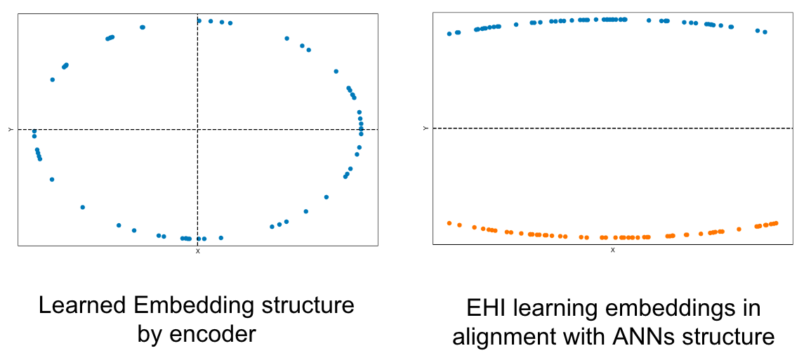
(a) Misalignment of representations

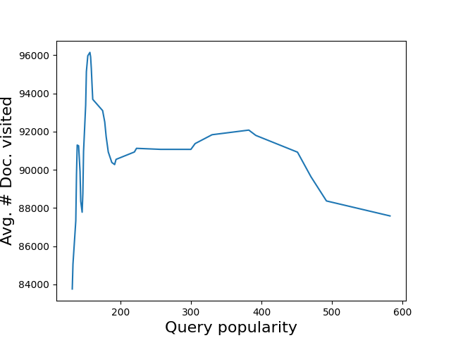
(b) Query Distribution MSMARCO

Figure 4: Motivation of EHI.

Appendix C Model and Hyperparameter details

We followed a standard approach called grid search to determine the optimal hyperparameters for training the ${\rm EHI}$ model. This involved selecting a subset of the training dataset and systematically exploring different combinations of hyperparameter values that perform best on this held-out set. The key hyperparameters we focused on were the Encoder ($\mathcal{E}_{\theta}$ ) and Indexer ($\mathcal{I}_{\phi}$) learning rates. Other hyperparameters to tune involved the weights assigned to each component of the loss function, denoted as $\lambda_{1},\lambda_{2},\lambda_{3}$ in Equation 6.

The specific hyperparameter values used in our experiments are detailed in Table 4. This table provides a comprehensive overview of the exact settings for each hyperparameter. The transformer block used in this work is the sentence transformers distilBERT model, which has been trained on the MSMarco dataset (https://huggingface.co/sentence-transformers/msmarco-distilbert-cos-v5). We fine-tune the encoder for our task and report our performance metrics.

Table 4: Hyperparameters used for training ${\rm EHI}$ on various datasets. Note that number of epoch and refresh rate ($r$) was set to 100 and 5, respectively. ${\rm EHI}$ initializes with distilBERT with encoder embedding representation as $768$

Description	Scifact	Fiqa	MSMarco	NQ320k	argument_name
General Settings
Batch size	$64$	$64$	$4096$	$1024$	batch_size
Number of leaves	$40$	$5000$	$7000$	$1000$	leaves
Optimizer Settings
Encoder Learning rate	$4e^{-4}$	$2e^{-4}$	$2.5e^{-8}$	$1e^{-4}$	enc_lr
Classifier Learning rate	$0.016$	$9e^{-4}$	$8e^{-3}$	$4e^{-4}$	cl_lr
Loss factor 1	$0.2$	$0.03$	$0.11$	$0.2$	$\lambda_{1}$
Loss factor 2	$0.8$	$0.46$	$0.84$	$0.4$	$\lambda_{2}$
Loss factor 3	$0.2$	$0.54$	$0.60$	$0.11$	$\lambda_{3}$

Appendix D Comparisons to SOTA

In this section, we compare ${\rm EHI}$ with SOTA approaches such as ColBERT, SGPT, cpt-text, ANCE, DyNNIBAL, which use different dot-product metrics or hard-negative mining mechanisms, etc. Note that ${\rm EHI}$ proposed in this paper is a paradigm shift of training and can be clubbed with any of the above architectures. So the main comparison is not with SOTA architectures, but it is against the existing paradigm of two-stage dense retrieval as highlighted in Section 4.2. Nevertheless, we showcase that ${\rm EHI}$ outperforms SOTA approaches on both MS MARCO dev set as well as MS MARCO TREC DL-19 setting as highlighted in Table 5 and Table 6 respectively.

Table 5: Performance metrics ($\%$) evaluated on the MS MARCO dev dataset. The best value for each metric is indicated in bold font.

Method	MRR@10 (Dev)	nDCG@10 (Dev)
DPR Thakur et al. (2021)	-	17.7
BM25 (official) Khattab & Zaharia (2020)	16.7	22.8
BM25 (Anserini) Khattab & Zaharia (2020)	18.7	-
cpt-text S Neelakantan et al. (2022)	19.9	-
cpt-text M Neelakantan et al. (2022)	20.6	-
cpt-text L Neelakantan et al. (2022)	21.5	-
cpt-text XL Neelakantan et al. (2022)	22.7	-
DSI (Atomic Docid + Doc2Query + Base Model) Tay et al. (2022)	26.0	32.28
DSI (Naive String Docid + Doc2Query + XL Model) Tay et al. (2022)	21.0	-
DSI (Naive String Docid + Doc2Query + XXL Model) Tay et al. (2022)	16.5	-
DSI (Semantic String Docid + Doc2Query + XL Model) Tay et al. (2022)	20.3	27.86
HNSW Malkov & Yashunin (2018)	28.9	-
RoBERTa-base + In-batch Negatives Monath et al. (2023)	24.2	-
RoBERTa-base + Uniform Negatives Monath et al. (2023)	30.5	-
RoBERTa-base + DyNNIBAL Monath et al. (2023)	33.4	-
RoBERTa-base + Stochastic Negatives Monath et al. (2023)	33.1	-
RoBERTa-base +Negative Cache Monath et al. (2023)	33.1	-
RoBERTa-base + Exhaustive Negatives Monath et al. (2023)	34.5	-
SGPT-CE-2.7B Muennighoff (2022)	-	27.8
SGPT-CE-6.1B Muennighoff (2022)	-	29.0
SGPT-BE-5.8B Muennighoff (2022)	-	39.9
doc2query Khattab & Zaharia (2020)	21.5	-
DeepCT Thakur et al. (2021)	24.3	29.6
docTTTTquery Khattab & Zaharia (2020)	27.7	-
SPARTA Thakur et al. (2021)	-	35.1
docT5query Thakur et al. (2021)	-	33.8
ANCE	33.0	38.8
EHI (distilbert-cos; Ours)	33.8	39.4
TAS-B Thakur et al. (2021)	-	40.8
GenQ Thakur et al. (2021)	-	40.8
ColBERT (re-rank) Khattab & Zaharia (2020)	34.8	-
ColBERT (end-to-end) Khattab & Zaharia (2020)	36.0	40.1
BM25 + CE Thakur et al. (2021)	-	41.3
EHI (distilbert-dot; Ours)	37.2	43.3

Table 6: Performance metrics ($\%$) evaluated on the MS MARCO TREC-DL 2019 Craswell et al. (2020) dataset. The best value for each metric is indicated in bold font.

Method	MRR@10	nDCG@10
BM25 Robertson et al. (2009)	68.9	50.1
Cross-attention BERT (12-layer) Menon et al. (2022)	82.9	74.9
Dual Encoder BERT (6-layer) Menon et al. (2022)	83.4	67.7
DistilBERT + MSE Menon et al. (2022)	78.1	69.3
DistilBERT + Margin MSE Menon et al. (2022)	86.7	71.8
DistilBERT + RankDistil-B Menon et al. (2022)	85.2	70.8
DistilBERT + Softmax CE Menon et al. (2022)	84.6	72.6
DistilBERT + $M^{3}$SE Menon et al. (2022)	85.2	71.4
EHI (distilbert-cos; Ours)	97.7	88.4

Table 7: Performance metrics ($\%$) evaluated on the NQ320$k$ dataset (Kwiatkowski et al., 2019). The best value for each metric is indicated in bold font.

Method	R@10	R@100
BM25 Robertson et al. (2009)	32.48	50.54
BERT + ANN (Faiss) Johnson et al. (2019)	53.63	73.01
BERT + BruteForce Wang et al. (2022)	53.42	73.16
BM25 + DocT5Query Nogueira et al. (2019)	61.83	76.92
ANCE (FirstP) Xiong et al. (2020)	80.33	91.78
ANCE (MaxP) Xiong et al. (2020)	80.38	91.31
SEAL (Base) Bevilacqua et al. (2022)	79.97	91.39
SEAL (Large) Bevilacqua et al. (2022)	81.24	91.93
RoBERTa-base + In-batch Negatives Monath et al. (2023)	69.5	84.3
RoBERTa-base + Uniform Negatives Monath et al. (2023)	72.3	84.8
RoBERTa-base + DyNNIBAL Monath et al. (2023)	75.4	86.2
RoBERTa-base + Stochastic Negatives Monath et al. (2023)	75.8	86.2
RoBERTa-base +Negative Cache Monath et al. (2023)	-	85.6
RoBERTa-base + Exhaustive Negatives Monath et al. (2023)	80.4	86.6
DSI (Base) Tay et al. (2022)	56.6	-
DSI (Large) Tay et al. (2022)	62.6	-
DSI (XXL) Tay et al. (2022)	70.3	-
NCI (Base) Wang et al. (2022)	85.2	92.42
NCI (Large) Wang et al. (2022)	85.27	92.49
NCI w/ qg-ft (Base) Wang et al. (2022)	88.48	94.48
NCI w/ qg-ft (Large) Wang et al. (2022)	88.45	94.53
EHI (distilbert-cos; Ours)	88.98	96.3

Appendix E Additional Experiments

This section presents additional experiments conducted on our proposed model, referred to as ${\rm EHI}$. The precise performance metrics of our model, as discussed in Section 4.2, are provided in Appendix E.1. This analysis demonstrates that our approach achieves state-of-the-art performance even with different initializations, highlighting its robustness (Appendix E.2).

Furthermore, we delve into the document-to-leaves ratio concept, showcasing its adaptability to degrees greater than one and the advantages of doing so, provided that our computational requirements are met (Appendix E.8). This flexibility allows for the exploration of more nuanced clustering possibilities. We also examine load balancing in ${\rm EHI}$ and emphasize the utilization of all leaves in a well-distributed manner. This indicates that our model learns efficient representations and enables the formation of finer-grained clusters (Appendix E.4).

To shed light on the learning process, we present the expected documents per leaf metric over the training regime in Appendix E.5. This analysis demonstrates how ${\rm EHI}$ learns to create more evenly distributed clusters as training progresses, further supporting its effectiveness.

Finally, we provide additional insights into the semantic analysis of the Indexer in Appendix E.8, highlighting the comprehensive examination performed to understand the inner workings of our model better.

Through these additional experiments and analyses, we reinforce the efficacy, robustness, and interpretability of our proposed ${\rm EHI}$ model, demonstrating its potential to advance the field of information retrieval.

E.1 Results on various benchmarks

In this section, we depict the precise numbers we achieve with various baselines as well as ${\rm EHI}$ as shown in Table 8, Table 9, and Table 10 for Scifact, Fiqa, and MS Marco respectively.

Table 8: Performance metrics ($\%$) evaluated on the Scifact dataset across various ranges of visited documents. The best value for each metric, corresponding to a specific number of visited documents, is indicated in bold font.

Metric	Method	10%	20%	30%	40%	50%	60%	70%	80%	90%	100%
R@$10$	Exact Search	75.82
	ScaNN	59.59	68.41	70.07	72.74	75.07	75.52	75.85	75.85	75.85	75.82
	Faiss-IVF	62.31	67.54	71.32	73.32	75.32	75.49	75.82	75.82	75.82	75.82
	EHI	76.97	81.93	83.33	83.67	84.73	85.07	84.73	84.73	84.73	84.73
R@$20$	Exact Search	82.93
	ScaNN	64.26	73.49	76.16	78.99	81.32	81.77	82.43	82.43	82.43	82.93
	Faiss-IVF	67.17	73.32	77.43	79.77	82.1	82.6	82.93	82.93	82.93	82.93
	EHI	81.03	85.27	86.5	86.17	87.23	87.57	87.57	87.57	87.57	87.57
R@$50$	Exact Search	87.9
	ScaNN	67.66	79.96	82.62	85.29	87.62	88.4	89.07	89.07	89.07	87.9
	Faiss-IVF	70.57	78.12	81.63	84.13	86.07	87.23	87.9	87.9	87.9	87.9
	EHI	82.87	88.67	91.73	92.07	93.2	93.53	93.53	93.53	93.87	93.87
R@$100$	Exact Search	91.77
	ScaNN	67.89	80.76	83.76	87.49	89.82	90.6	91.6	91.27	91.27	91.77
	Faiss-IVF	71.81	79.42	83.93	86.93	89.6	91.1	91.77	91.77	91.77	91.77
	EHI	83.53	89.33	92.9	93.23	94.43	94.77	94.77	94.93	95.27	95.27

To understand how the performance of ${\rm EHI}$ model is on a smaller number of $k$ in Recall@$k$, we report Recall@$10$, Recall@$25$, and Recall@$50$ metrics on the Scifact dataset. Figure 6 depicts the performance of the ${\rm EHI}$ model in this setting. On the Recall@$10$, Recall@$20$ and Recall@$50$ metric, ${\rm EHI}$ outperforms exact search metric by $8.91\%$, $4.64\%$ and $5.97\%$ respectively.

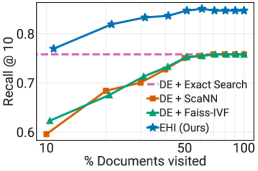
(a) Scifact - R@10

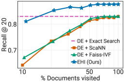
(b) Scifact - R@20

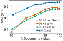
(c) Scifact - R@50

Figure 6: Additional Results for other Recall@k metrics of EHI trained on the Scifact dataset.

Table 9: Performance metrics ($\%$) evaluated on the Fiqa dataset across various ranges of visited documents. The best value for each metric, corresponding to a specific number of visited documents, is indicated in bold font.

Metric	Method	10%	20%	30%	40%	50%	60%	70%	80%	90%	100%
R@$10$	Exact Search	30.13
	ScaNN	23.95	29.08	29.69	29.98	29.83	30.13	30.08	30.08	30.13	30.13
	Faiss-IVF	26.8	29.67	29.9	29.93	29.93	29.93	29.98	30.13	30.13	30.13
	EHI	27.43	32.02	32.12	32.19	32.42	32.42	32.42	32.42	32.47	32.47
R@$20$	Exact Search	36.0
	ScaNN	28.54	34.45	35.34	35.67	35.7	36.0	35.88	35.95	36.0	36.0
	Faiss-IVF	32.17	35.51	35.77	35.8	35.8	35.8	35.85	36.0	36.0	36.0
	EHI	33.47	39.01	39.36	39.45	39.68	39.68	39.68	39.68	39.73	39.73
R@$50$	Exact Search	45.4
	ScaNN	35.93	43.38	44.51	45.11	45.02	45.12	45.07	45.48	45.5	45.4
	Faiss-IVF	39.78	44.45	44.86	45.19	45.19	45.19	45.24	45.4	45.4	45.4
	EHI	41.03	49.77	50.35	50.62	50.75	50.83	50.99	50.99	51.04	51.04
R@$100$	Exact Search	53.78
	ScaNN	51.0	51.9	52.33	52.69	52.63	53.39	52.49	52.97	53.64	53.78
	Faiss-IVF	52.75	53.27	53.65	53.65	53.65	53.63	53.78	53.78	53.78	53.78
	EHI	57.36	58.42	58.97	59.18	59.13	59.29	59.29	59.34	59.34	59.39

Table 10: Performance metrics ($\%$) evaluated on the MS Marco dataset across various ranges of visited documents. The best value for each metric, corresponding to a specific number of visited documents, is indicated in bold font.

Metric	Method	10%	20%	30%	40%	50%	60%	70%	80%	90%	100%
nDCG@$1$	Exact Search	22.41
	ScaNN	22.06	22.38	22.36	22.36	22.41	22.39	22.41	22.41	22.41	22.41
	Faiss-IVF	22.16	22.32	22.38	22.41	22.41	22.41	22.39	22.39	22.39	22.41
	EHI	22.39	22.48	22.46	22.46	22.46	22.46	22.46	22.46	22.46	22.46
nDCG@$3$	Exact Search	32.5
	ScaNN	31.96	32.36	32.42	32.43	32.49	32.48	32.5	32.5	32.5	32.5
	Faiss-IVF	32.05	32.25	32.39	32.44	32.48	32.48	32.48	32.5	32.5	32.5
	EHI	32.45	32.61	32.61	32.6	32.6	32.6	32.6	32.6	32.6	32.6
nDCG@$5$	Exact Search	36.03
	ScaNN	35.38	35.82	35.91	35.94	36.01	36.01	36.03	36.02	36.03	36.03
	Faiss-IVF	35.56	35.75	35.89	35.96	36.0	36.0	36.02	36.04	36.04	36.03
	EHI	35.9	36.08	36.08	36.08	36.08	36.08	36.08	36.08	36.08	36.08
nDCG@$10$	Exact Search	39.39
	ScaNN	38.61	39.1	39.25	39.3	39.37	39.36	39.38	39.38	39.39	39.39
	Faiss-IVF	38.86	39.09	39.23	39.31	39.35	39.36	39.36	39.38	39.38	39.39
	EHI	39.19	39.42	39.42	39.42	39.43	39.43	39.43	39.43	39.43	39.43
MRR@$10$	Exact Search	33.77
	ScaNN	33.16	33.58	33.67	33.7	33.76	33.75	33.77	33.77	33.77	33.77
	Faiss-IVF	33.34	33.54	33.66	33.72	33.75	33.75	33.74	33.76	33.76	33.77
	EHI	33.64	33.81	33.81	33.8	33.81	33.8	33.8	33.8	33.8	33.8

Furthermore, we note that most prior works, including ScaNN, DSI, and NCI, all report their numbers for a single seed. To show the robustness of our approach to initializations, we also report our numbers on multiple seeds and showcase that we significantly outperform our baselines across all the boards as further described in Section E.2.

E.2 Robustness to initializations

In this section, we showcase the robustness of our proposed approach - ${\rm EHI}$  to various initializations of the model. Note that analysis in this manner is uncommon in efficient retrieval works, as showcased in ScaNN, DSI, and NCI. However, such approaches worked with two disjoint processes for learning embeddings, followed by the ANNS. Since we attempt to solve the problem in an end-to-end framework in a differentiable fashion through neural networks, it is worth understanding the effect of different initializations or seeds on our learning. Overall, we run the same model for the best hyperparameters over five different seeds and report the mean and standard deviation numbers below in Table 11.

Table 11: Performance metrics ($\%$) evaluated on the various datasets across various ranges of visited documents. The best value for each metric, corresponding to a specific number of visited documents, is indicated in bold font. Here, $n$ denotes the number of seeds run for the given model. We report the mean and standard deviation of the metrics for ${\rm EHI}$ and showcase a robustness to initialization.

Metric	Method	10%	20%	30%	40%	50%	60%	70%	80%	90%	100%
Scifact - R@$100$	Exact Search	91.77
	ScaNN	67.89	80.76	83.76	87.49	89.82	90.6	91.6	91.27	91.27	91.77
	Faiss-IVF	71.81	79.42	83.93	86.93	89.6	91.1	91.77	91.77	91.77	91.77
	EHI ($n=5$)	80.68 $\pm$ 1.51	87.05 $\pm$ 1.92	90.06 $\pm$ 0.97	91.75 $\pm$ 0.89	93.03 $\pm$ 0.77	93.26 $\pm$ 0.72	93.34 $\pm$ 0.73	93.44 $\pm$ 0.62	93.51 $\pm$ 0.62	93.51 $\pm$ 0.62
Fiqa - R@$100$	Exact Search	53.78
	ScaNN	51.0	51.9	52.33	52.69	52.63	53.39	52.49	52.97	53.64	53.78
	Faiss-IVF	52.75	53.27	53.65	53.65	53.65	53.63	53.78	53.78	53.78	53.78
	EHI ($n=5$)	57.23 $\pm$ 0.42	57.74 $\pm$ 0.27	57.91 $\pm$ 0.27	57.98 $\pm$ 0.26	58.07 $\pm$ 0.25	58.08 $\pm$ 0.24	58.11 $\pm$ 0.21	58.11 $\pm$ 0.21	58.1 $\pm$ 0.22	58.1 $\pm$ 0.22
MS Marco - nDCG@$10$	Exact Search	39.39
	ScaNN	38.61	39.1	39.25	39.3	39.37	39.36	39.38	39.38	39.39	39.39
	Faiss-IVF	38.86	39.09	39.23	39.31	39.35	39.36	39.36	39.38	39.38	39.39
	EHI ($n=5$)	39.17 $\pm$ 0.04	39.34 $\pm$ 0.03	39.39 $\pm$ 0.02	39.41 $\pm$ 0.01	39.41 $\pm$ 0.01	39.42 $\pm$ 0.01	39.42 $\pm$ 0.01	39.42 $\pm$ 0.01	39.42 $\pm$ 0.01	39.42 $\pm$ 0.01
MSMarco - MRR@$10$	Exact Search	33.77
	ScaNN	33.16	33.58	33.67	33.7	33.76	33.75	33.77	33.77	33.77	33.77
	Faiss-IVF	33.34	33.54	33.66	33.72	33.75	33.75	33.74	33.76	33.76	33.77
	EHI ($n=5$)	33.62 $\pm$ 0.03	33.74 $\pm$ 0.03	33.77 $\pm$ 0.02	33.78 $\pm$ 0.01	33.78 $\pm$ 0.01	33.79 $\pm$ 0.01	33.79 $\pm$ 0.01	33.79 $\pm$ 0.01	33.79 $\pm$ 0.01	33.79 $\pm$ 0.01

E.3 Statistical Significance Tests

In this section, we aim to show that the improvements achieved by ${\rm EHI}$ over other baselines as depicted in Sec 4.2 are statistically significant. We confirm with hypothesis tests that all the results on datasets considered in this work are statistically significant with a p-value less than 0.05.

Table 12: Statistical Significance p-test.

Dataset	Scifact (R@100)	Fiqa (R@100)	MSMARCO (nDCG@10)	MSMARCO (MRR@10)
p-value	0.0016	7.97E-07	0.0036	0.0018

E.4 Load balancing

Load balancing is a crucial objective that we aim to accomplish in this work. By achieving nearly uniform clusters, we can create clusters with finer granularity, ultimately reducing latency in our model. In Figure 7(a), we can observe the distribution of documents across different leaf nodes. It is noteworthy that the expected number of documents per leaf, calculated as $\sum_{i=1}^{l=\#\text{Leaf}}p_{i}c_{i}$, where $p_{i}$ represents the probability of a document in bucket index $i$ and $c_{i}$ denotes the number of documents in bucket $i$, yields an optimal value of approximately $1263.12$. Currently, our approach attains an expected number of documents per leaf of $1404.65$. Despite a slight skewness in the distribution, we view this as advantageous since we can allocate some leaves to store infrequently accessed tail documents from our training dataset. Additionally, our analysis demonstrates that queries are roughly evenly divided, highlighting the successful load balancing achieved, as illustrated in Figure 7.

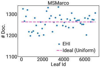
(a) MS MARCO: Document load balancing

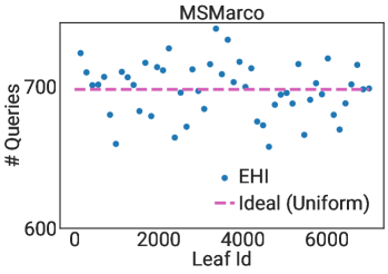
(b) MS MARCO: Query load balancing

Figure 7: Leaf distribution of documents and queries of MS Marco in our trained ${\rm EHI}$ model. Our model learns splits closer to ideal split (uniform), this suggests that all the leaves are efficiently used, and our model does not learn very lob sided clusters. This roughly uniform spread of both queries (Figure 7(b)), as well as documents (Figure 7(a)) provides a more fine-grained clustering structure which not only takes advantage of all the leaves but also shows state of the art performance compared to baselines as discussed extensively in Section 4.2.

E.5 Learning to balance load over epochs

In the previous section, we showed that our learned clusters are almost uniformly distributed, and help improve latency as shown in Section 4.2. In this section, we study the progression of expected documents per leaf as defined above over training progression on the Scifact dataset. In Figure 8 demonstrates the decline of the expected documents per leaf over the training regime.

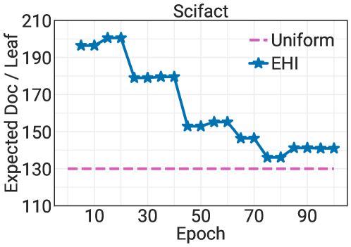
Figure 8: Load balancing of documents over the training regime of ${\rm EHI}$. ${\rm EHI}$ learning objective encourages well balances leaf nodes as well as state of the art accuracy.

E.6 Scaling to deeper trees

In this section, we further motivate the need to extend to deep trees and showcase how this extension is critical to be deployed in production. We show that the hierarchical part in ${\rm EHI}$ is absolutely necessary for two reasons:

Sub-optimal convergence and blow-up in path embedding:

When working with hundreds of billions of scale datasets as ones generally used in industry, a single height indexer would not work. Having more than a billion logits returned by a single classification layer would be suboptimal and lead to poor results. This is a common trend observed in other domains, such as Extreme Classification, and thus warrants hierarchy in our model design. Furthermore, the path embedding would blow up if we use a single height indexer, and optimization and gradient alignments would become the bottleneck in this scenario.

Sub-linear scaling and improved latency:

Furthermore, increasing the height of ${\rm EHI}$ can be shown to scale to very large leaves and documents. Consider a case where our encoder has $P$ parameters, and the indexer is a single height tree that tries to index each document of $D$ dimension into $L$ leaves. The complexity of forward pass in this setting would be $\mathcal{O}(P+DL)$. However, for very large values of $L$, this computation could blow up and lead to suboptimal latency and blow up in memory. Note, however, that by extending the same into multiple leaves ($H$), one can reduce the complexity at each height to a sublinear scale. The complexity of forward pass the hierarchical k-ary tree would be $\mathcal{O}(P+HDL^{1/H})$. Note that since $L\gg H$, the hierarchical k-ary tree can be shown to have a better complexity and latency, which helps in scaling to documents of the scale of billions as observed in general applications in real-world scenarios. For instance, ${\rm EHI}$ trained on Scifact with equal number of leaves, we notice a significant speedup with increasing height; for example at $(B=64,H=1)$, $(B=8,H=2)$, and $(B=4,H=3)$, we notice a per-query latency of $2.48ms$, $2.40ms$, and $1.99ms$ respectively at the same computation budget.

In the above results presented in Section 4.3, we showcase that one could increase the depth of the tree to allow multiple linear layers of lower logits - say 1000 clusters at each height instead of doing so at a single level. This is precisely where the hierarchical part of the method is absolutely necessary for scalability. Furthermore, we also extend ${\rm EHI}$ model on other datasets such as Scifact to showcase this phenomenon as depicted in Table 13. We do confirm with a p-test with a p-value of 0.05 and confirm that the results across different permutations are nearly identical, and the improvements on R@50 and R@100 over other permutations are not statistically significant (improvements < 0.5%). Furthermore, improvements of other permutations of (B,H) on the R@10 and R@20 metrics over the H=1 baseline are also statistically insignificant. Our current experiments on Scifact/MSMARCO not only portray that our method does indeed scale to deeper trees but also showcase that ${\rm EHI}$ can extend to deeper trees with little to no loss in performance and improved latency.

Table 13: Performance metrics ($\%$) evaluated on the Scifact dataset across various permutations of braching factor (B) and height (H). The best value for each metric, corresponding to a specific number of visited documents, is indicated in bold font.

Scifact	R@10	R@20	R@50	R@100
Two-tower model (with Exact Search)	75.82	82.93	87.9	91.77
${\rm EHI}$ (B=40, H=1)	84.73	87.57	93.87	95.27
${\rm EHI}$ (B=4, H=2)	86.23	88.7	93.43	94.77
${\rm EHI}$ (B=6, H=2)	83.8	88.63	92.77	95.27
${\rm EHI}$ (B=8, H=2)	84.46	88.47	93.27	95.27
${\rm EHI}$ (B=4, H=3)	84.96	88.7	93.6	94.77
${\rm EHI}$ (B=6, H=3)	85.36	89.3	93.6	94.77
${\rm EHI}$ (B=8, H=3)	83.86	87.47	92.27	95.27

E.7 Effect of negative mining refresh rate

Finally, we study the accuracy of ${\rm EHI}$ when increasing the frequency of negative mining refresh rate ($r$) to extend its effectiveness in accurately indexing extensive web-scale document collections. In the experiments presented earlier in Section 4.2, we took a design choice where we mined hard negatives once every five epochs. This negative mining is particularly expensive since this requires computing the clusters every time for all the documents/passages - of the order 8.8M in MS MARCO, which could possibly add a 30% or higher overhead in our training time. Although one could reduce the frequency of negative mining to help convergence, it would be slower to train. Some preliminary studies in this regime are shown in Figure 9, where mining hard negatives more frequently leads to an improved recall metric of $1.4\%$.

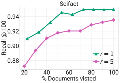
Figure 9: Figure illustrating the effect of negative mining refresh factor ($r$) on the downstream performance of ${\rm EHI}$ on the Scifact dataset.

E.8 Allowing documents to have multiple semantics

Note that throughout training, our model works with a beam size for both query and document and tries to send relevant documents and queries to the same leaves. While testing, we have only presented results where beam size is used to send queries to multiple leaves, limiting the number of leaves per document to 1. We could use a number of leaves per document as a hyperparameter and allow documents to reach multiple leaves as long as our computational power allows.

Accuracy:

In this section, we extend our results on increasing this factor on the MS Marco dataset as presented in Figure 10. Intuitively, each document could have multiple views, and simply sending them to only one leaf might not be ideal, but efficient indexing. Furthermore, increasing this hyperparameter from the default $d2l=1$ setting shows strictly superior performance and improves our metrics on the MRR@$10$ as well as nDCG@$10$ metric.

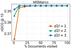
(a) MS MARCO: nDCG@10

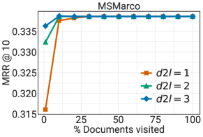
(b) MS MARCO: MRR@10

Figure 10: Ablation study of docs to leaves on the MS Marco benchmark. Overall, we notice that as long as computational power is available, increasing number of leaves indexed for documents aids performance in retrieval.

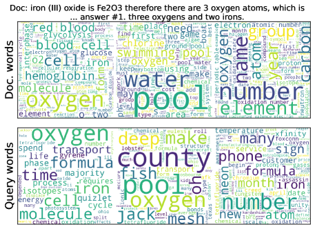
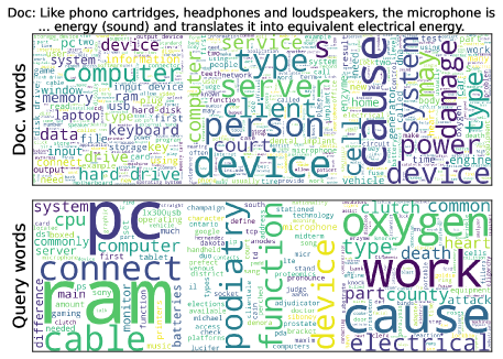
Figure 11: We deploy the concept of word cloud to summarize the semantics of all queries and documents in a leaf. Here, every document and query can hold multiple semantics therefore for the analysis, each document ($Doc$) was assigned to multiple leafs with decreasing order of similarity. It can be seen that for each leaf captures slightly different semantic for the document. On further observations, queries that were mapped to the same leaf also shares the semantic similarity with the $Doc$. Note that semantic similarity decreases as the relevance of document to a label decreases (left to right). This shows that ${\rm EHI}$’s training objection (Part 2 and Part 3) ensure queries with similar semantic meaning as document as as well as similar documents are clustered together.

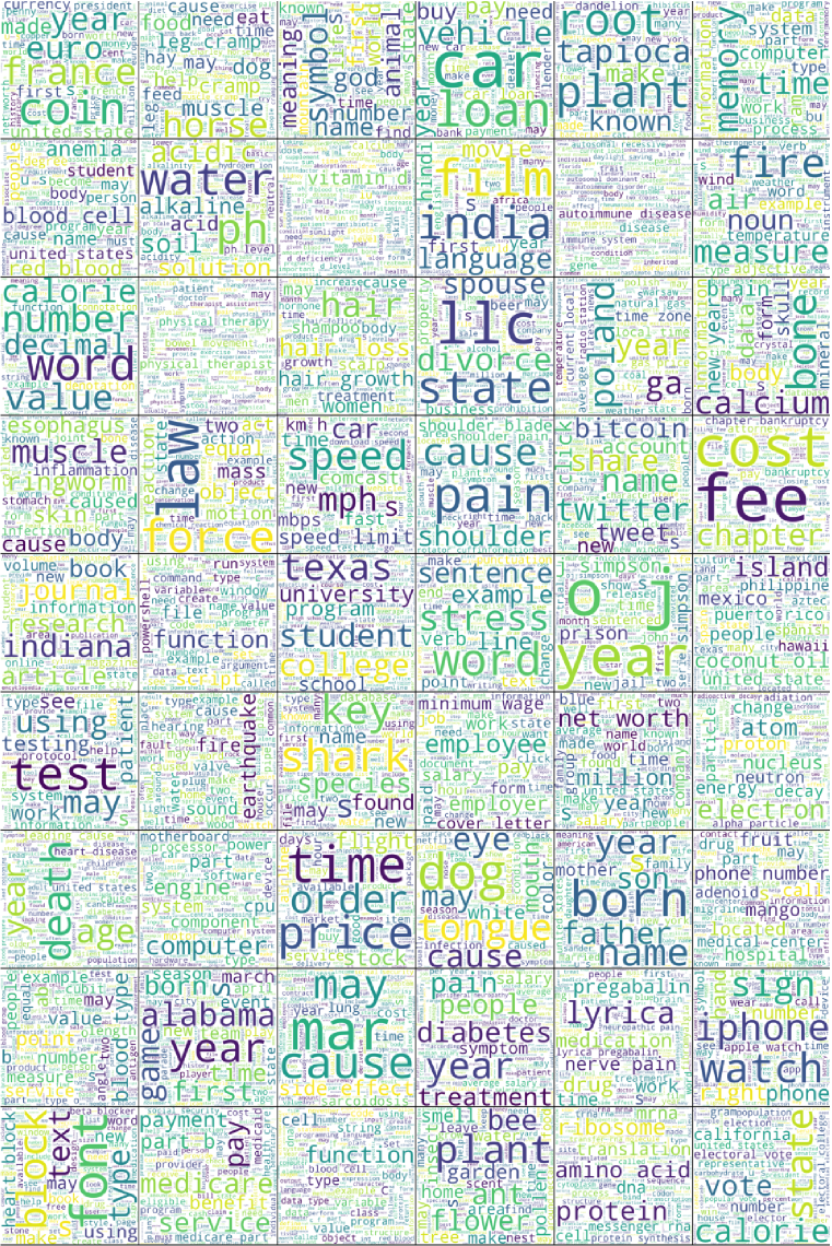
Figure 12: Figure shows that ${\rm EHI}$’s learning objective encourages leaf nodes to have different semantics. Here semantic information in each leaf is shown in the form of word cloud. The seemingly similar leaves such as (1,1), (5, 5) or (8,2) shares the similar words like “year” however, they capture completely different meaning such as financial, criminal and sports respectively.

Advantages of Multiple Leaves per Document:

While assigning a document to multiple leaf nodes incurs additional memory costs, we uncover intriguing semantic properties from this approach. For the analysis, we assign multiple leaves for a document ($Doc$) ranked based on decreasing order of similarity, as shown in Figure 11. For Figure 11, we showcase three distinct examples of diverse domains showcasing not only the semantic correlation of the documents which reach similar leaves but also the queries which reach the same leaf as our example. It can be seen that each leaf captures slightly different semantics for the document. On further observations, queries mapped to the same leaf also share the semantic similarity with the $Doc$. Note that semantic similarity decreases as the document’s relevance to a label decreases (left to right). This shows that ${\rm EHI}$’s training objection (Part 2 and Part 3) ensures queries with similar semantic meaning as documents and similar documents are clustered together.

Diverse Concepts Across Leaf Nodes:

Our analysis, as showcased in Figure 12, reveals a wide range of diverse concepts captured by the word clouds derived from the leaf nodes of${\rm EHI}$. For Figure 12, we visualize only a subset of randomly chosen leaves (54) instead of all leaf nodes clarity, which was obtained through random sampling. Below, we highlight some intriguing findings from our analysis. These concepts span various domains such as phones, plants, healthcare, judiciary, and more. Moreover, within each leaf node, we observe a cohesive theme among the words. For instance, the word cloud at coordinates $(1,1)$ reflects an international finance theme, while the word cloud at $(1,2)$ pertains to fitness. This observation highlights the importance of grouping similar documents into the same leaf nodes and excluding irrelevant documents using our objective function. Note that seemingly similar leaves such as $(1,1)$, $(5,5)$, or $(8,2)$ share similar words like “year”; however, they capture completely different meanings such as financial, criminal, and sports, respectively.

Algorithm 1 Training step for ${\rm EHI}$. $\mathbf{u}(q)$ & $\mathbf{v}(d)$ denote the query (q) & document (d) representation from encoder $\mathcal{E}_{\theta}$. Similarly path embedding by the indexer ($\mathcal{I}_{\phi}$) is denoted by $\mathcal{T}(q)$ & $\mathcal{T}(d)$. Please refer to Algorithm 2 in appendix for the definition of TOPK-INDEXER and INDEXER

$\phi\leftarrow$ Indexer Parameters, $\theta\leftarrow$ Encoder parameters, $\tau\leftarrow$ similarity threshold, $B\leftarrow$ indexer branching factor, $H\leftarrow$ indexer height, $\beta\leftarrow$ beam size, $\mathcal{M}\leftarrow$ Mapping of leaf to documents, $\hat{\mathcal{Q}}=\{q_{1},q_{2},\dots,q_{s}\}\sim\mathcal{Q}$ (randomly sampled mini-batch), INDEXER $\leftarrow$ Returns path embedding, TOPK-INDEXER $\leftarrow$ Returns most relevant leaf

procedure RETRIEVER($\mathbf{u}$, $\phi$, $\beta$) – Retrieves most relevant doc

     $\_,\_,\text{Leafs}=\texttt{TOPK-INDEXER}(\mathbf{u},\phi,B,H,\beta)$ $\triangleright$ Refer to Alg 2

     return $\cup_{l\in\text{Leafs}}\mathcal{M}(l)$

end procedure

procedure Training($\hat{Q}$) – jointly update encoder and indexer parameters $\theta$, $\phi$

     $\mathbf{loss}$ = 0

     for $q_{i}\in\hat{\mathcal{Q}}$ do

         $d_{i}\sim\{k|\mathbf{y}_{ik}=1\}$ $\triangleright$ Sample a relevant document

         $h_{i}\sim\{d|\texttt{RETRIEVER}(\mathcal{E}_{\theta}(q_{i}),\phi,\beta)\}\setminus\{k|\mathbf{y}_{ik}=1\}$$\triangleright$ Sample a hard neg. from retriever

         $\mathbf{loss}\mathrel{+}=\mathcal{L}(\mathcal{E}_{\theta}(q_{i}),\mathcal{E}_{\theta}(d_{i}),\mathcal{E}_{\theta}(h_{i}))$ $\triangleright$ Triplet loss against hard negative

         for $q_{j}\in\hat{\mathcal{Q}}$ and $q_{i}\neq q_{j}$ do

              $d_{j}\sim\{k|\mathbf{y}_{ik}=-1\cap\mathbf{y}_{jk}=1\}$ $\triangleright$ Sample an in-batch negative

              $\mathbf{loss}\mathrel{+}=\mathcal{L}(\mathcal{E}_{\theta}(q_{i}),\mathcal{E}_{\theta}(d_{i}),\mathcal{E}_{\theta}(d_{j}))$ $\triangleright$ Uses $\theta$ to encode doc. and query

              $\mathbf{loss}\mathrel{+}=\mathcal{L}(\mathcal{T}_{\phi}(q_{i}),\mathcal{T}_{\phi}(d_{i}),\mathcal{T}_{\phi}(d_{j}))$$\triangleright$ Uses INDEXER in Alg 2 for $\mathcal{T}_{\phi}$.

              $\mathbf{loss}\mathrel{+}=\mathbf{1}\{\texttt{SIM}(\mathbf{v}(d_{i}),\mathbf{v}(d_{j}))<\tau\}\mathcal{L}(\mathcal{T}_{\phi}(d_{i}),\mathcal{T}_{\phi}(d_{i}),\mathcal{T}_{\phi}(d_{j}))$

         end for

     end for

     return $\texttt{Update}(\theta,\phi,\mathbf{loss})$ $\triangleright$ Update encoder and indexer parameters with gradient of loss

end procedure

Algorithm 2 Training step for ${\rm EHI}$. $\mathbf{u}(q)$ & $\mathbf{v}(d)$ denote the query (q) & document (d) representation from encoder $\mathcal{E}_{\theta}$. Similarly path embedding by the indexer ($\mathcal{I}_{\phi}$) is denoted by $\mathcal{T}(q)$ & $\mathcal{T}(d)$.

$\phi=\{\mathbf{W}_{H},\dots,\mathbf{W}_{1},\mathbf{U}_{H},\dots,\mathbf{U}_{1}\}\leftarrow$ Indexer Parameters, $\theta\leftarrow$ Encoder parameters, $\tau\leftarrow$ Inter-document similarity threshold, $B\leftarrow$ branching factor of the Indexer, $H\leftarrow$ height of the indexer, $\beta\leftarrow$ beam size, $\mathcal{M}\leftarrow$ Mapping of leaf to documents, $\hat{\mathcal{Q}}=\{q_{1},q_{2},\dots,q_{s}\}\sim\mathcal{Q}$ (randomly sampled mini-batch)

procedure INDEXER($\mathbf{u},\phi,B,H$) – Computes indexer path emb. for a query/document

     $l=$ TOPK-INDEXER($\mathbf{u},\phi,B,H,\beta=1$)

     $\mathcal{T}_{\phi}=[]$

     $p_{l}=1$

     for  $h\in 1\dots H$  do

         $\hat{\mathbf{p}}=\mathcal{S}([\mathbf{o}(i^{h-1}_{l});\mathbf{o}(i^{h-2}_{l});\dots;\mathbf{o}(i^{1}_{l});\mathbf{u}];\mathbf{W}_{h},\mathbf{U}_{h})$

         $\mathcal{T}_{\phi}=[\mathcal{T}_{\phi};\hat{\mathbf{p}}\cdot p_{l}]$

         $p_{l}=p_{l}\cdot\hat{\mathbf{p}}[i^{h}_{l}]$

     end for

     return $\mathcal{T}_{\phi}$

end procedure

procedure TOPK-INDEXER($\mathbf{u},\phi,B,H,\beta$) – Indexes a query/document in the $\beta$ most relevant leaves

     $h\leftarrow 1$, $\mathcal{P}=\{<1,\mathbf{u},0>\}$ $\triangleright$ Tuple of score, path and node ID

     while  $h\leq H$  do

         $\hat{\mathcal{P}}=\texttt{Max-Heap}(size=\beta)$

         for $s,\mathbf{p},n\in\mathcal{P}.pop()$ do

              $\hat{\mathbf{p}}=\mathcal{S}(\mathbf{p};\mathbf{W}_{h},\mathbf{U}_{h})\times s$; For all $i\in 1\dots B$: $\hat{\mathcal{P}}.push(<\hat{\mathbf{p}}[i],\mathbf{o}(i);\mathbf{p},n\cdot B+i>)$

         end for

         $\mathcal{P}=\hat{\mathcal{P}}$

     end while

     return $\mathcal{P}$

end procedure

References

- Bajaj et al. (2016) Payal Bajaj, Daniel Campos, Nick Craswell, Li Deng, Jianfeng Gao, Xiaodong Liu, Rangan Majumder, Andrew McNamara, Bhaskar Mitra, Tri Nguyen, et al. Ms marco: A human generated machine reading comprehension dataset. arXiv preprint arXiv:1611.09268, 2016.
- Bernhardsson (2018) Erik Bernhardsson. Annoy: Approximate Nearest Neighbors in C++/Python, 2018. URL https://pypi.org/project/annoy/. Python package version 1.13.0.
- Bevilacqua et al. (2022) Michele Bevilacqua, Giuseppe Ottaviano, Patrick Lewis, Scott Yih, Sebastian Riedel, and Fabio Petroni. Autoregressive search engines: Generating substrings as document identifiers. Advances in Neural Information Processing Systems, 35:31668–31683, 2022.
- Beygelzimer et al. (2006) Alina Beygelzimer, Sham Kakade, and John Langford. Cover trees for nearest neighbor. In Proceedings of the 23rd international conference on Machine learning, pp. 97–104, 2006.
- Cai (2021) Deng Cai. A revisit of hashing algorithms for approximate nearest neighbor search. IEEE Transactions on Knowledge and Data Engineering, 33(6):2337–2348, 2021. doi: 10.1109/TKDE.2019.2953897.
- Chopra et al. (2005) Sumit Chopra, Raia Hadsell, and Yann LeCun. Learning a similarity metric discriminatively, with application to face verification. In 2005 IEEE computer society conference on computer vision and pattern recognition (CVPR’05), volume 1, pp. 539–546. IEEE, 2005.
- Clarkson (1994) Kenneth L Clarkson. An algorithm for approximate closest-point queries. In Proceedings of the tenth annual symposium on Computational geometry, pp. 160–164, 1994.
- Craswell et al. (2020) Nick Craswell, Bhaskar Mitra, Emine Yilmaz, Daniel Campos, and Ellen M Voorhees. Overview of the trec 2019 deep learning track. arXiv preprint arXiv:2003.07820, 2020.
- Dahiya et al. (2021) Kunal Dahiya, Deepak Saini, Anshul Mittal, Ankush Shaw, Kushal Dave, Akshay Soni, Himanshu Jain, Sumeet Agarwal, and Manik Varma. Deepxml: A deep extreme multi-label learning framework applied to short text documents. In Proceedings of the 14th ACM International Conference on Web Search and Data Mining, pp. 31–39, 2021.
- Datar et al. (2004) Mayur Datar, Nicole Immorlica, Piotr Indyk, and Vahab S Mirrokni. Locality-sensitive hashing scheme based on p-stable distributions. In Proceedings of the twentieth annual symposium on Computational geometry, pp. 253–262, 2004.
- Devlin et al. (2018) Jacob Devlin, Ming-Wei Chang, Kenton Lee, and Kristina Toutanova. Bert: Pre-training of deep bidirectional transformers for language understanding. arXiv preprint arXiv:1810.04805, 2018.
- Eksombatchai et al. (2018) Chantat Eksombatchai, Pranav Jindal, Jerry Zitao Liu, Yuchen Liu, Rahul Sharma, Charles Sugnet, Mark Ulrich, and Jure Leskovec. Pixie: A system for recommending 3+ billion items to 200+ million users in real-time. In Proceedings of the 2018 world wide web conference, pp. 1775–1784, 2018.
- Friedman et al. (1977) Jerome H Friedman, Jon Louis Bentley, and Raphael Ari Finkel. An algorithm for finding best matches in logarithmic expected time. ACM Transactions on Mathematical Software (TOMS), 3(3):209–226, 1977.
- Gao et al. (2020) Luyu Gao, Zhuyun Dai, Zhen Fan, and Jamie Callan. Complementing lexical retrieval with semantic residual embedding. corr abs/2004.13969 (2020). arXiv preprint arXiv:2004.13969, 2020.
- Ge et al. (2013) Tiezheng Ge, Kaiming He, Qifa Ke, and Jian Sun. Optimized product quantization. IEEE transactions on pattern analysis and machine intelligence, 36(4):744–755, 2013.
- Guo et al. (2020) Ruiqi Guo, Philip Sun, Erik Lindgren, Quan Geng, David Simcha, Felix Chern, and Sanjiv Kumar. Accelerating large-scale inference with anisotropic vector quantization. In International Conference on Machine Learning, pp. 3887–3896. PMLR, 2020.
- Gupta et al. (2022) Nilesh Gupta, Patrick Chen, Hsiang-Fu Yu, Cho-Jui Hsieh, and Inderjit Dhillon. Elias: End-to-end learning to index and search in large output spaces. Advances in Neural Information Processing Systems, 35:19798–19809, 2022.
- Gutmann & Hyvärinen (2010) Michael Gutmann and Aapo Hyvärinen. Noise-contrastive estimation: A new estimation principle for unnormalized statistical models. In Proceedings of the thirteenth international conference on artificial intelligence and statistics, pp. 297–304. JMLR Workshop and Conference Proceedings, 2010.
- Guu et al. (2020) Kelvin Guu, Kenton Lee, Zora Tung, Panupong Pasupat, and Mingwei Chang. Retrieval augmented language model pre-training. In International conference on machine learning, pp. 3929–3938. PMLR, 2020.
- Huggingface (2019) Huggingface. HuggingFace Sentence-transformers for MSMarco, 2019. URL https://huggingface.co/sentence-transformers/msmarco-distilbert-cos-v5.
- Indyk & Motwani (1998) Piotr Indyk and Rajeev Motwani. Approximate nearest neighbors: towards removing the curse of dimensionality. In Proceedings of the thirtieth annual ACM symposium on Theory of computing, pp. 604–613, 1998.
- Izacard & Grave (2020a) Gautier Izacard and Edouard Grave. Distilling knowledge from reader to retriever for question answering. arXiv preprint arXiv:2012.04584, 2020a.
- Izacard & Grave (2020b) Gautier Izacard and Edouard Grave. Leveraging passage retrieval with generative models for open domain question answering. arXiv preprint arXiv:2007.01282, 2020b.
- Izacard et al. (2021) Gautier Izacard, Mathilde Caron, Lucas Hosseini, Sebastian Riedel, Piotr Bojanowski, Armand Joulin, and Edouard Grave. Towards unsupervised dense information retrieval with contrastive learning. arXiv preprint arXiv:2112.09118, 2021.
- Izacard et al. (2022) Gautier Izacard, Patrick Lewis, Maria Lomeli, Lucas Hosseini, Fabio Petroni, Timo Schick, Jane Dwivedi-Yu, Armand Joulin, Sebastian Riedel, and Edouard Grave. Few-shot learning with retrieval augmented language models. arXiv preprint arXiv:2208.03299, 2022.
- Jain et al. (2019) Himanshu Jain, Venkatesh Balasubramanian, Bhanu Chunduri, and Manik Varma. Slice: Scalable linear extreme classifiers trained on 100 million labels for related searches. In Proceedings of the Twelfth ACM International Conference on Web Search and Data Mining, pp. 528–536, 2019.
- Jaiswal et al. (2022) Shikhar Jaiswal, Ravishankar Krishnaswamy, Ankit Garg, Harsha Vardhan Simhadri, and Sheshansh Agrawal. Ood-diskann: Efficient and scalable graph anns for out-of-distribution queries. arXiv preprint arXiv:2211.12850, 2022.
- Jayaram Subramanya et al. (2019) Suhas Jayaram Subramanya, Fnu Devvrit, Harsha Vardhan Simhadri, Ravishankar Krishnawamy, and Rohan Kadekodi. Diskann: Fast accurate billion-point nearest neighbor search on a single node. Advances in Neural Information Processing Systems, 32, 2019.
- Jegou et al. (2010) Herve Jegou, Matthijs Douze, and Cordelia Schmid. Product quantization for nearest neighbor search. IEEE transactions on pattern analysis and machine intelligence, 33(1):117–128, 2010.
- Johnson et al. (2019) Jeff Johnson, Matthijs Douze, and Hervé Jégou. Billion-scale similarity search with GPUs. IEEE Transactions on Big Data, 7(3):535–547, 2019.
- Khattab & Zaharia (2020) Omar Khattab and Matei Zaharia. Colbert: Efficient and effective passage search via contextualized late interaction over bert. In Proceedings of the 43rd International ACM SIGIR conference on research and development in Information Retrieval, pp. 39–48, 2020.
- Kolesnikov et al. (2020) Alexander Kolesnikov, Lucas Beyer, Xiaohua Zhai, Joan Puigcerver, Jessica Yung, Sylvain Gelly, and Neil Houlsby. Big transfer (bit): General visual representation learning. In Computer Vision–ECCV 2020: 16th European Conference, Glasgow, UK, August 23–28, 2020, Proceedings, Part V 16, pp. 491–507. Springer, 2020.
- Kumar et al. (2023) Ramnath Kumar, Kushal Majmundar, Dheeraj Nagaraj, and Arun Sai Suggala. Stochastic re-weighted gradient descent via distributionally robust optimization. arXiv preprint arXiv:2306.09222, 2023.
- Kusupati et al. (2021) Aditya Kusupati, Matthew Wallingford, Vivek Ramanujan, Raghav Somani, Jae Sung Park, Krishna Pillutla, Prateek Jain, Sham Kakade, and Ali Farhadi. Llc: Accurate, multi-purpose learnt low-dimensional binary codes. Advances in Neural Information Processing Systems, 34:23900–23913, 2021.
- Kusupati et al. (2022) Aditya Kusupati, Gantavya Bhatt, Aniket Rege, Matthew Wallingford, Aditya Sinha, Vivek Ramanujan, William Howard-Snyder, Kaifeng Chen, Sham Kakade, Prateek Jain, et al. Matryoshka representation learning. Advances in Neural Information Processing Systems, 35:30233–30249, 2022.
- Kwiatkowski et al. (2019) Tom Kwiatkowski, Jennimaria Palomaki, Olivia Redfield, Michael Collins, Ankur Parikh, Chris Alberti, Danielle Epstein, Illia Polosukhin, Jacob Devlin, Kenton Lee, et al. Natural questions: a benchmark for question answering research. Transactions of the Association for Computational Linguistics, 7:453–466, 2019.
- Li et al. (2020) W Li, Y Zhang, Y Sun, W Wang, W Zhang, and X Lin. Approximate nearest neighbor search on high dimensional data—experiments, analyses, and improvement. IEEE Transactions on Knowledge and Data Engineering, 2020.
- Loshchilov & Hutter (2017) Ilya Loshchilov and Frank Hutter. Decoupled weight decay regularization. arXiv preprint arXiv:1711.05101, 2017.
- Maia et al. (2018) Macedo Maia, Siegfried Handschuh, André Freitas, Brian Davis, Ross McDermott, Manel Zarrouk, and Alexandra Balahur. Www’18 open challenge: financial opinion mining and question answering. In Companion proceedings of the the web conference 2018, pp. 1941–1942, 2018.
- Malkov & Yashunin (2020) Yu A Malkov and DA Yashunin. Efficient and robust approximate nearest neighbor search using hierarchical navigable small world graphs. IEEE Transactions on Pattern Analysis & Machine Intelligence, 42(04):824–836, 2020.
- Malkov & Yashunin (2018) Yu A Malkov and Dmitry A Yashunin. Efficient and robust approximate nearest neighbor search using hierarchical navigable small world graphs. IEEE transactions on pattern analysis and machine intelligence, 42(4):824–836, 2018.
- Menon et al. (2022) Aditya Menon, Sadeep Jayasumana, Ankit Singh Rawat, Seungyeon Kim, Sashank Reddi, and Sanjiv Kumar. In defense of dual-encoders for neural ranking. In International Conference on Machine Learning, pp. 15376–15400. PMLR, 2022.
- Mitra et al. (2018) Bhaskar Mitra, Nick Craswell, et al. An introduction to neural information retrieval. Foundations and Trends® in Information Retrieval, 13(1):1–126, 2018.
- Monath et al. (2023) Nicholas Monath, Manzil Zaheer, Kelsey Allen, and Andrew McCallum. Improving dual-encoder training through dynamic indexes for negative mining. In International Conference on Artificial Intelligence and Statistics, pp. 9308–9330. PMLR, 2023.
- Muennighoff (2022) Niklas Muennighoff. Sgpt: Gpt sentence embeddings for semantic search. arXiv preprint arXiv:2202.08904, 2022.
- Nayak (2019) Pandu Nayak. Understanding searches better than ever before. Google AI Blog, 2019. URL https://blog.google/products/search/search-language-understanding-bert/.
- Neelakantan et al. (2022) Arvind Neelakantan, Tao Xu, Raul Puri, Alec Radford, Jesse Michael Han, Jerry Tworek, Qiming Yuan, Nikolas Tezak, Jong Wook Kim, Chris Hallacy, et al. Text and code embeddings by contrastive pre-training. arXiv preprint arXiv:2201.10005, 2022.
- Ni et al. (2021) Jianmo Ni, Chen Qu, Jing Lu, Zhuyun Dai, Gustavo Hernández Ábrego, Ji Ma, Vincent Y Zhao, Yi Luan, Keith B Hall, Ming-Wei Chang, et al. Large dual encoders are generalizable retrievers. arXiv preprint arXiv:2112.07899, 2021.
- Nogueira & Cho (2019) Rodrigo Nogueira and Kyunghyun Cho. Passage re-ranking with bert. arXiv preprint arXiv:1901.04085, 2019.
- Nogueira et al. (2019) Rodrigo Nogueira, Wei Yang, Jimmy Lin, and Kyunghyun Cho. Document expansion by query prediction. arXiv preprint arXiv:1904.08375, 2019.
- Qu et al. (2020) Yingqi Qu, Yuchen Ding, Jing Liu, Kai Liu, Ruiyang Ren, Wayne Xin Zhao, Daxiang Dong, Hua Wu, and Haifeng Wang. Rocketqa: An optimized training approach to dense passage retrieval for open-domain question answering. arXiv preprint arXiv:2010.08191, 2020.
- Radford et al. (2018) Alec Radford, Karthik Narasimhan, Tim Salimans, Ilya Sutskever, et al. Improving language understanding by generative pre-training. OpenAI, 2018.
- Radford et al. (2021) Alec Radford, Jong Wook Kim, Chris Hallacy, Aditya Ramesh, Gabriel Goh, Sandhini Agarwal, Girish Sastry, Amanda Askell, Pamela Mishkin, Jack Clark, et al. Learning transferable visual models from natural language supervision. In International conference on machine learning, pp. 8748–8763, 2021.
- Reimers & Gurevych (2019) Nils Reimers and Iryna Gurevych. Sentence-bert: Sentence embeddings using siamese bert-networks. arXiv preprint arXiv:1908.10084, 2019.
- Robertson et al. (2009) Stephen Robertson, Hugo Zaragoza, et al. The probabilistic relevance framework: Bm25 and beyond. Foundations and Trends® in Information Retrieval, 3(4):333–389, 2009.
- Salakhutdinov & Hinton (2009) Ruslan Salakhutdinov and Geoffrey Hinton. Semantic hashing. International Journal of Approximate Reasoning, 50(7):969–978, 2009.
- Sivic & Zisserman (2003) Josef Sivic and Andrew Zisserman. Video google: A text retrieval approach to object matching in videos. In Computer Vision, IEEE International Conference on, volume 3, pp. 1470–1470. IEEE Computer Society, 2003.
- Tay et al. (2022) Yi Tay, Vinh Tran, Mostafa Dehghani, Jianmo Ni, Dara Bahri, Harsh Mehta, Zhen Qin, Kai Hui, Zhe Zhao, Jai Gupta, et al. Transformer memory as a differentiable search index. Advances in Neural Information Processing Systems, 35:21831–21843, 2022.
- Thakur et al. (2021) Nandan Thakur, Nils Reimers, Andreas Rücklé, Abhishek Srivastava, and Iryna Gurevych. Beir: A heterogenous benchmark for zero-shot evaluation of information retrieval models. arXiv preprint arXiv:2104.08663, 2021.
- Wadden et al. (2020) David Wadden, Shanchuan Lin, Kyle Lo, Lucy Lu Wang, Madeleine van Zuylen, Arman Cohan, and Hannaneh Hajishirzi. Fact or fiction: Verifying scientific claims. arXiv preprint arXiv:2004.14974, 2020.
- Wang et al. (2021) Mengzhao Wang, Xiaoliang Xu, Qiang Yue, and Yuxiang Wang. A comprehensive survey and experimental comparison of graph-based approximate nearest neighbor search. Proceedings of the VLDB Endowment, 14(11):1964–1978, 2021.
- Wang et al. (2022) Yujing Wang, Yingyan Hou, Haonan Wang, Ziming Miao, Shibin Wu, Qi Chen, Yuqing Xia, Chengmin Chi, Guoshuai Zhao, Zheng Liu, et al. A neural corpus indexer for document retrieval. Advances in Neural Information Processing Systems, 35:25600–25614, 2022.
- Weber et al. (1998) Roger Weber, Hans-Jörg Schek, and Stephen Blott. A quantitative analysis and performance study for similarity-search methods in high-dimensional spaces. In VLDB, volume 98, pp. 194–205, 1998.
- Xiong et al. (2020) Lee Xiong, Chenyan Xiong, Ye Li, Kwok-Fung Tang, Jialin Liu, Paul Bennett, Junaid Ahmed, and Arnold Overwijk. Approximate nearest neighbor negative contrastive learning for dense text retrieval. arXiv preprint arXiv:2007.00808, 2020.