TOI-5126: A hot super-Neptune and warm Neptune pair discovered by TESS and CHEOPS

Abstract

We present the confirmation of a hot super-Neptune with an exterior Neptune companion orbiting a bright (V = 10.1 mag) F-dwarf identified by the Transiting Exoplanet Survey Satellite (TESS). The two planets, observed in sectors 45, 46 and 48 of the TESS extended mission, are $4.74_{-0.14}^{+0.16}$$R_{\earth}$ and $3.86_{-0.16}^{+0.17}$$R_{\earth}$ with $5.4588385_{-0.0000072}^{+0.0000070}$ d and $17.8999_{-0.0013}^{+0.0018}$ d orbital periods, respectively. We also obtained precise space based photometric follow-up of the system with ESA’s CHaracterising ExOplanets Satellite (CHEOPS) to constrain the radius and ephemeris of TOI-5126 b. TOI-5126 b is located in the ‘hot Neptune Desert’ and is an ideal candidate for follow-up transmission spectroscopy due to its high predicted equilibrium temperature ($T_{\rm eq}$= ${1442}_{-40}^{+46}$ K) implying a cloud-free atmosphere. TOI-5126 c is a warm Neptune ($T_{\rm eq}$= $971_{-27}^{+31}$ K) also suitable for follow-up. Tentative transit timing variations (TTVs) have also been identified in analysis, suggesting the presence of at least one additional planet, however this signal may be caused by spot-crossing events, necessitating further precise photometric follow-up to confirm these signals.

1 Introduction

Super-Neptunes are a class of planets potentially bridging the gap between Neptune and Jovian planets (4-8 $R_{\earth}$). Despite being of similar sizes, they exhibit a significant diversity in mass, almost uniformly distributed between 6 and 135 $M_{\earth}$ (Akeson et al., 2013; Petigura et al., 2017). Given the absence of such planets in the Solar system, studying the population provides extra insights on the versatility of the planet formation process around other stars.

An archetypal example of the super-Neptune class is GJ 436 b (Gillon et al., 2007). It has a Neptune-like radius coupled with a relatively high density. It also has an inferred rocky element core and substantial H/He envelope (Fortney et al., 2007). Its characteristics appear to deviate from the theorised $\approx$ 5 $M_{\earth}$ threshold needed for runaway accretion (Lee & Chiang, 2016a), highlighting our lack of understanding about the formation channels from which this class originates. Kepler and the subsequent K2 mission (Borucki et al., 2010; Howell et al., 2014) enabled the first population studies of these planets. Petigura et al. (2017) proposed that super-Neptunes form in gas-depleted disks (Lee et al., 2014) or from planet-planet mergers (Petigura et al., 2017). Both of these formation scenarios lead to heavy elements in the planets atmosphere, making these theories testable with bright systems hosting super-Neptunes.

However, the majority of confirmed super-Neptunes discovered by the Kepler and K2 missions orbit around relatively faint stars, posing challenges for detailed atmosphere characterisation. The all-sky Transiting Exoplanet Survey Satellite (TESS, Ricker et al. 2015) mission aims to survey the entire sky for candidates around some of the brightest nearby stars, providing the best opportunity to further our knowledge of super-Neptunes. TESS has already identified several unique super-Neptunes, including LTT 9779 b (Jenkins et al., 2020a) and TOI-849 b (Armstrong et al., 2020). Both reside in the ‘hot Neptune desert’ (Mazeh et al., 2016), creating further challenges to their formation and evolution models. Planets in this close-in highly irradiated period space are usually thought to be most susceptable to photoevaporation (Owen & Jackson, 2012; Jin et al., 2014; Lopez, 2017) and tidal stripping (Matsakos & Königl, 2016; Owen & Lai, 2018). LTT 9779 b is an ideal target for follow-up atmospheric studies, with a Spitzer phase curve already suggesting a high-metallicity atmosphere (Crossfield et al., 2020). Efforts to understand this population can be most fruitful via multiplanet systems, where comparative planetology is possible.

In this paper, we present the discovery of a multi-transiting system around the F-dwarf ($T_{\rm eff}$$=$ $6150_{-100}^{+130}$ K) TOI-5126. The system, first discovered by TESS, hosts a hot super-Neptune located in the ‘hot Neptune Desert’, and an exterior warm Neptune. The brightness of TOI-5126 and the high predicted equilibrium temperatures of planet b (${1442}_{-40}^{+46}$ K) and c ($971_{-27}^{+31}$ K) make these planets ideal for future follow-up, including atmospheric comparative planetology studies. In section §2, we present the photometric, imaging and spectroscopic observations that led to the discovery and confirmation of the TOI-5126 system. Section §3 discusses the derived stellar parameters of TOI-5126, as well as the global modeling and analysis of the system. The results of our analysis are presented in section §4, including validation of TOI-5126 b and TOI-5126 c, transit timing variations (TTVs), and future follow-up opportunities.

2 Observations and Data analysis

2.1 Photometry

2.1.1 TESS

TOI-5126 (TIC 27064468) was observed by TESS nearly continuously on both the 2 min cadence target pixel stamps and the 10 min FFIs in sectors 45 (Camera 3 CCD 4) and 46 (Camera 2 CCD 2), with an additional sector (sector 48, Camera 1 CCD 4) a month later. The observations were taken from UT 2021-Nov-06 to UT 2022-Feb-26, for a total of $\approx$76 days.

In sector 46, systematic errors were observed in the first 13 hours of data due to a pointing adjustment . To mitigate these errors, we utilised quality flags to mask out scattered light and other systematic effects in the light curves .

The light curves  of TOI-5126 were processed by both the TESS Science Processing Operations Center (SPOC; Jenkins et al. 2016), located at NASA Ames Research Center. The SPOC conducted a transit search of Sector 45 2-min cadence data on UT 2021-Jan-09 with an adaptive, noise-compensating matched filter (Jenkins et al., 2002, 2010, 2020b), producing a Threshold Crossing Event (TCE) for which an initial limb-darkened transit model was fitted (Li et al., 2019) and a suite of diagnostic tests were conducted to help make or break the planetary nature of the signal (Twicken et al., 2018). Transit signatures were also detected in a search of Full Frame Image (FFI) 10-min cadence data by the Quick Look Pipeline (QLP) at MIT (Huang et al., 2020). The TESS Science Office (TSO) reviewed the vetting information and issued an alert for TOI-5126 b on UT 2022-Jan-25 based and an alert for TOI-5126 c on UT 2022-Feb-08 (Guerrero et al., 2021) based on QLP data. The signals were repeatedly recovered as additional observations were made including in both Sectors 46 and 48, as well as SPOC multi-sector searches (42-46, 14-50). The transit signatures again passed all the diagnostic tests presented in the Data Validation reports. Specifically, difference images from the Sectors 42-46 data located the catalog location of TOI-5126 b and TOI-5126 c within $9.0\pm{5.0}$ ″ and $5.2\pm{5.8}$ ″ of the transit source. The latest SPOC results captured signals for planets b (Signal-to-Noise (SNR): 26.1; Multiple Event Statistic (MES): 19.9) and c (SNR: 10.4; MES: 9.9). The transit events of TOI-5126 b were also identified by the Planet Hunters TESS citizen science project (Eisner et al., 2020) and uploaded to exoFOP as communitiy objects of interest (CTOI) on UT 2022-Jan-12.

For our analysis, a modification of the deblended SPOC Simple Aperture Photometry (SAP) light curves  (Twicken et al., 2010; Morris et al., 2020) were used in modeling (see Figure 1). Stellar variability was accounted for by simultaneously fitting for a polynomial trend around each transit as part of our global analysis. Two transits were manually excluded due to them occurring near a data gap. Our ephemeris and radius precision did not noticeably suffer from these excluded transits. The details of the global fit will be presented in section §3.2.

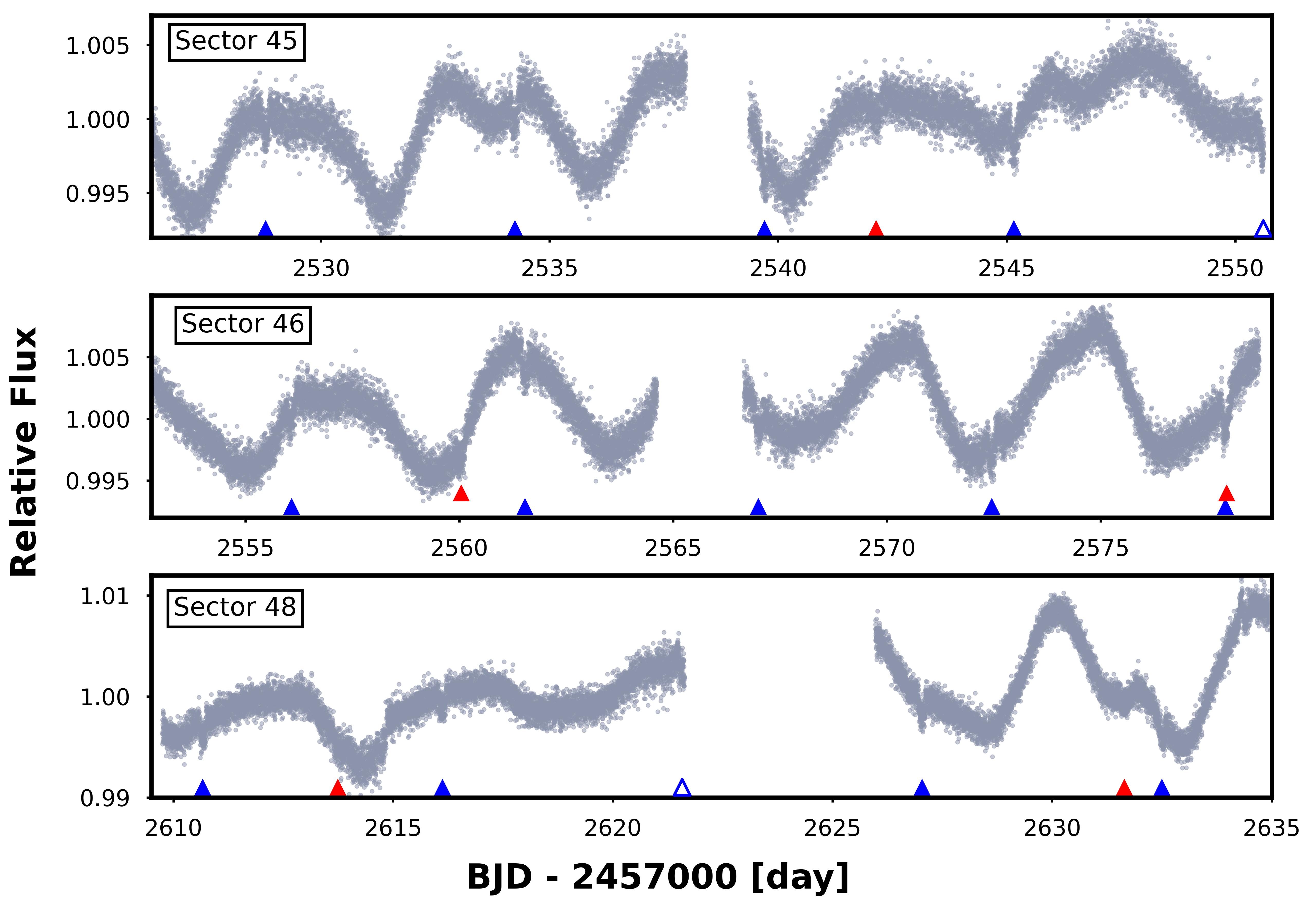
Figure 1: TESS SPOC SAP light curve  of TOI-5126 from all observed sectors. Blue triangles mark each transit of TOI-5126 b, with red arrows for transits of TOI-5126 c. Empty triangles indicate the transits not used in global modeling.

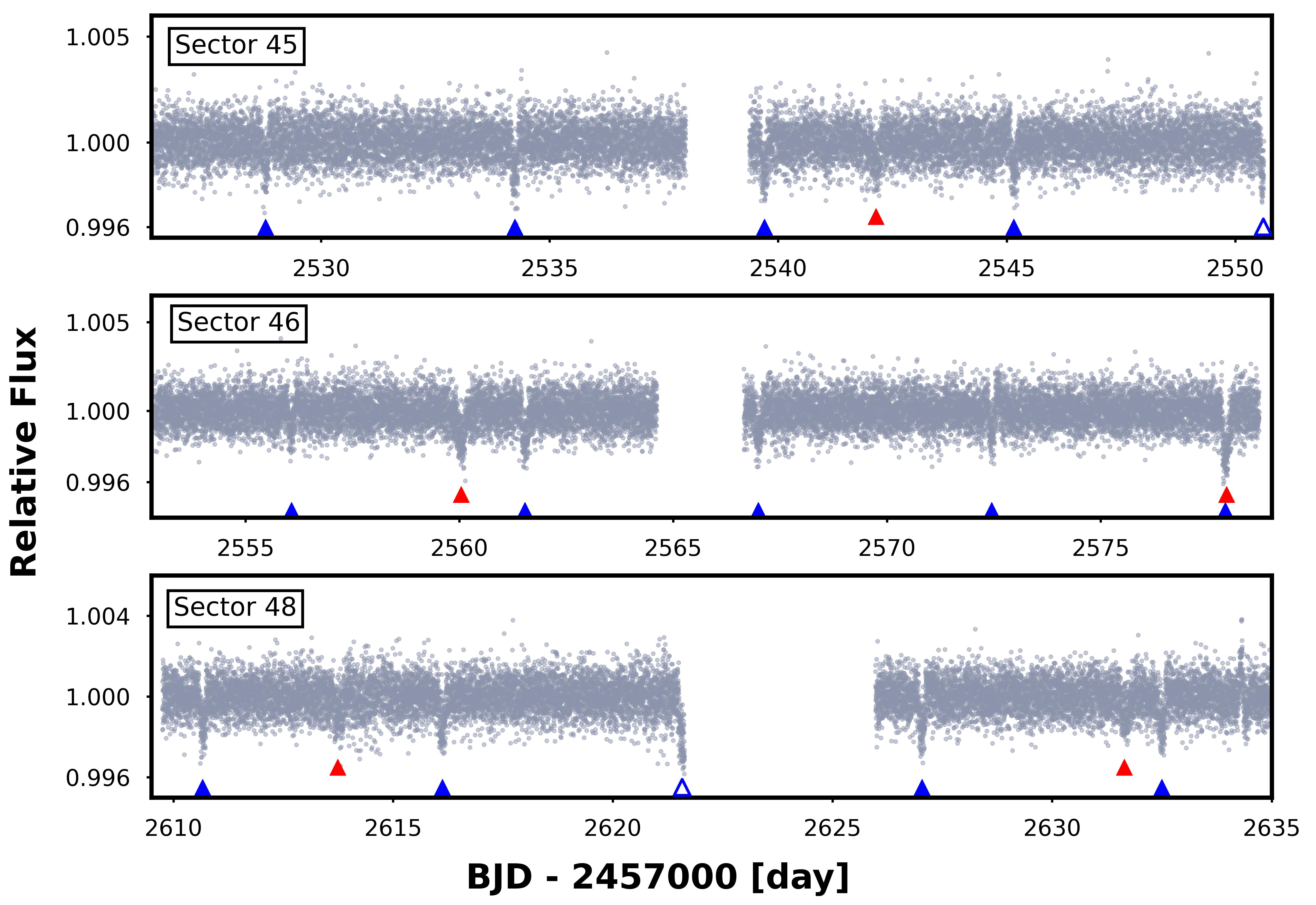
Figure 2: Detrended TESS light curve  of TOI-5126 from all observed sectors. The light curves are detrended using an iterative B-spline method, and are not used in the global modeling that lead to the final constraint of the planet parameters. Blue triangles mark each transit of TOI-5126 b, with red arrows for transits of TOI-5126 c. Empty triangles indicate the transits not used in global modeling.

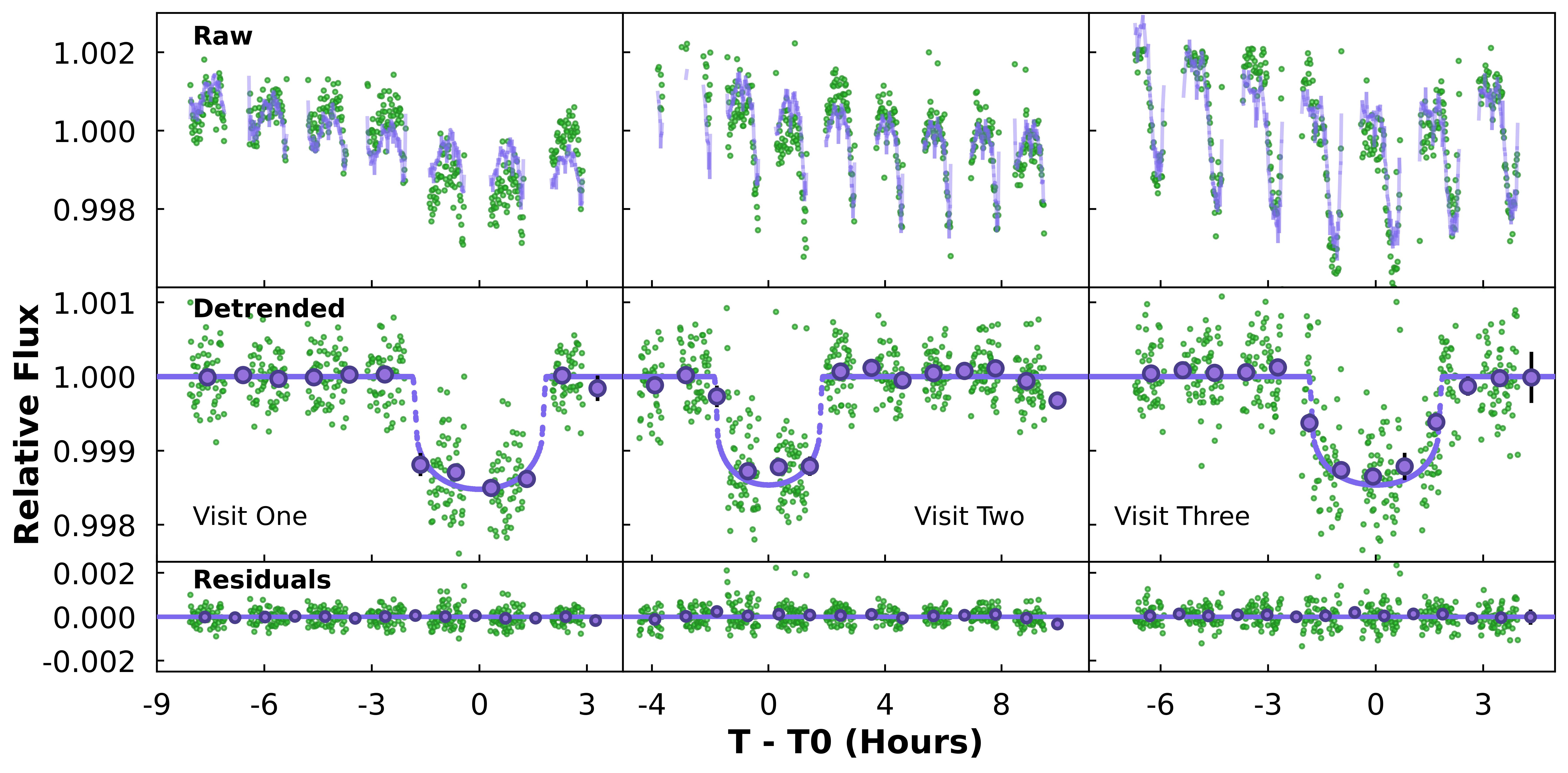
Figure 3: Upper: Raw normalised CHEOPS light curves  indicated by green points with the best-fit trend model plotted in purple. Middle: Detrended CHEOPS light curves  shown in green. Binned points are denoted as purple markers and the best-fit transit model is overplotted as a purple line. Lower: Residuals of the detrended light curves  in green, with binned averaged points shown in purple.

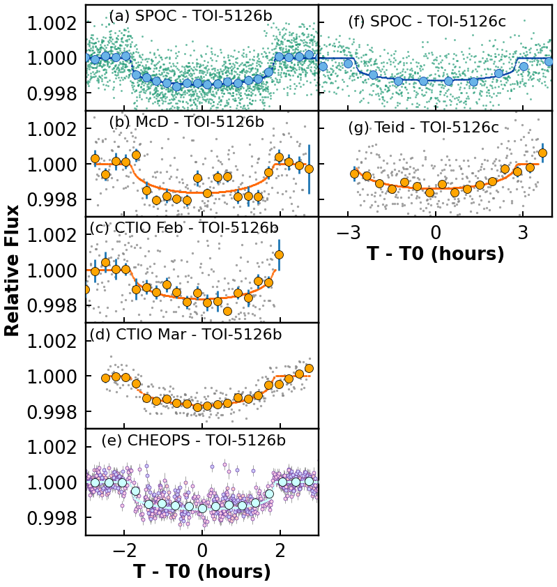
Figure 4: Phase-folded light curves  of TOI-5126 b and TOI-5126 c. TESS SPOC light curves  are noted by green points, with binned data in blue and the best-fit transit model line in blue. LCOGT data is represented by gray points with orange binned points and errorsbars in blue. The transit model is also denoted as an orange line. The CHEOPS phase folded light curve  is combined with all three visits TOI-5126 b, where the purple, pink and blue points represent each visit respectively. The binned data is in cyan, with the transit model also a cyan line. (a) TESS SPOC TOI-5126 b. (b) McD TOI-5126 b. (c) CTIO 2022 TOI-5126 b. (d) CTIO 2023 TOI-5126 b. (e) CHEOPS combined visits of TOI-5126 b. (f) TESS SPOC TOI-5126 c. (g) Teid TOI-5126 c.

2.1.2 CHEOPS

To refine the radius and ephemeris of TOI-5126 b, we obtained space-based photometric observations with CHEOPS (Benz et al., 2021). Observations were attained through the CHEOPS Guest Observers Programme (AO3-023). A first observation of TOI-5126 b occurred on 2022-02-16 21:44 UT for a duration of 11.72 hours. The preliminary data was processed through the CHEOPS Data Reduction Pipeline (version 13.1; Hoyer et al. 2020) on 2023-Feb-17 18:46 UT. The visit consisted of seven CHEOPS orbits, with a four orbit pre-ingress and one orbit post-egress out-of-transit baseline. An additional visit of TOI-5126 b occurred on 2023-Feb-27 23:55 UT in an attempt to identify an ingress/egress with high efficiency, resulting in an longer 14.14 hour observation, with two orbits pre-ingress and five orbits post-egress. We obtained a third visit of TOI-5126 b on 2023-Mar-27 04:44 where we successfully caught both the ingress and egress over an observation duration of 10.96 hours. The full details of observations are listed in Table 1.

The raw CHEOPS light curves  were detrended simultaneously with the transit modeling to best incorporate and propagate the uncertainties associated with the instrument into our final system parameters. Observations with poor data quality flags, and those that fail an iterative 5-$\sigma$ outlier rejection, were rejected from subsequent analyses. To correct for the CHEOPS systematics, we followed the trend model in the Pycheops package (Maxted et al., 2022). This model fits for spacecraft and environmental variations, including the roll angle, $\phi$, the background flux, bg, the contamination in the aperture, contam, smearing correction, smear and the x and y point spread function (PSF) centroid coordinates, dx $\&$ dy. The raw CHEOPS light curves  were detrended by fitting a least-squares model to the light curve residuals, which provided us with the best parameters for the trend model. These parameters were then applied to the trend function and subtracted from the raw flux to provide us with the detrended CHEOPS light curves , seen in Figure 3.

Table 1: List of CHEOPS Observations

Planet	Start Date [UT]	Duration [hours]	Valid Points [#]	File Key	Efficiency [%]	Exp. Time [s]
b	2023-02-16 21:44	11.72	422	CH_PR230023_TG000301_V0200	59.20	60.0
b	2023-02-27 23:55	14.14	549	CH_PR230023_TG000302_V0200	64.60	60.0
b	2023-03-27 04:44	10.96	458	CH_PR230023_TG000501_V0200	65.30	60.0

2.1.3 Ground based photometric follow up

Due to the coarse angular resolution of both TESS and CHEOPS, eclipsing binary stars within their apertures may mimic a transit event on the target star. To confirm the on-target detection of TOI-5126, we obtained ground-based photometric observations of both planets. We used the TESS Transit Finder, which is a customized version of the Tapir software package (Jensen, 2013), to schedule our transit observations. TOI-5126 b was observed in the $z_{s}$ filter by two 1.0 m Las Cumbres Observatory Global Network (LCOGT; Brown et al. 2013) telescopes simultaneously at the McDonald Observatory (McD) in Fort Davis, Texas (2022-Mar-10 UT). The transit event was detected with a depth of $\sim$1.8 ppt. The transit occured $\sim$12 minutes late (possibly caused by TTVs, see Section §4.3.3) and the field was cleared of Nearby Eclipsing Binaries in a 5.8″ aperture. An ingress was also observed by the 1.0 m telescope at the Cerro Tololo Inter-American Observatory (CTIO) in Cerro Tololo, Chile (2022-Apr-01 UT), however, this was not used in subsequent analysis and modeling of the system. TOI-5126 c was also observed with two 1.0 m LCOGT telescopes simultaneously at the Teide Observatory (Teid) in Tenerife, Spain on 2022-Apr-01 UT. A transit event was detected ($\sim$0.6 ppt) $\sim$57 minutes late after double-detrending with a variable aperture of 4.7″ and 3.1″. Two additional full transits of TOI-5126 b were obtained by the 1.0 m telescope at CTIO (2023-Feb-17 UT & 2023-Mar-15 UT). Both full coverages resulted in $\sim$1.2 ppt detections in an uncontaminated 4.7″ aperture. Table 2 provides the details of observation.

The images were calibrated by the standard LCOGT BANZAI pipeline (McCully et al., 2018) and differential photometric data were extracted using AstroImageJ (Collins et al., 2017). We opted to perform our own detrending of all LCOGT light curves  simultaneous to the global fit. The trend function for the light curves  were represented by a second-order polynomial, with an additional term counting for the full width half maximum of the PSF. As with the CHEOPS trend model, the coefficients of the detrending vectors were derived from a least squares fit that was performed at each iteration of the global modeling process.

Table 2: SG1 Follow-Up Observations

Target	Instrument	Date (UT)	Filter	Aperture	Observing Notes
TOI-5126 c	LCO-Teid 1.0m	2022-03-10	$z_{s}$	5.8″	Full coverage, simultaneous observation a
TOI-5126 c	LCO-Teid 1.0m	2022-03-10	$z_{s}$	4.7″	Full coverage, simultaneous observation a
TOI-5126 b	LCO-McD 1.0m	2022-04-01	$z_{s}$	5.8″	Full coverage, simultaneous observation b
TOI-5126 b	LCO-McD 1.0m	2022-04-01	$z_{s}$	4.7″	Full coverage, simultaneous observation b
TOI-5126 b	LCO-CTIO 1.0m	2022-04-01	$z_{s}$	3.9″	Ingress only, not included in global analysis
TOI-5126 b	LCO-CTIO 1.0m	2023-02-17	$z_{s}$	4.7″	Full coverage
TOI-5126 b	LCO-CTIO 1.0m	2023-03-15	$z_{s}$	4.7″	Full coverage

2.2 Reconnaissance Spectroscopy

We obtained a series of spectroscopic observations to check for contaminating spectroscopic blend scenarios, and to better constrain the spectroscopic atmospheric parameters of the target star. These reconnaissance spectroscopic observations are detailed in Table 3 and seen in Figure 5.

We obtained three spectra of TOI-5126 using the Tillinghast Reflector Echelle Spectrograph (TRES; Fűrész et al. 2008) on the 1.5 m telescope at the Fred Lawrence Whipple Observatory (Mt. Hopkins, Arizona). TRES has a resolving power of R $\simeq$ 44,000, with a wavelength coverage of 3850 to 9096 Å. The observations were obtained with an average exposure SNR per resolution element of 38 at 5110 Å. Radial velocities are derived from a multi-order cross correlation analysis as per Quinn et al. (2012), and spectroscopic parameters were derived via the Spectroscopic Parameter Classification tool (Buchhave et al., 2010). Observations yielded stellar parameters for effective temperature ($T_{\rm eff}$ = $6217\pm 50$ K), stellar surface gravity ($\log g$ = $4.3\pm 0.1$ cgs), metallicity ([Fe/H] = $0.17\pm 0.08$ dex) and projected rotation velocity ($v\sin I_{\star}$= $14.8\pm 0.5$ $\rm km\,s^{-1}$).

In addition, we also obtained five observations of TOI-5126 with the CHIRON high resolution spectrograph, located on the 1.5 m SMARTS telescope at Cerro Tololo Inter-American Observatory (CTIO), Chile (Tokovinin et al., 2013). Observations were obtained using the fiber fed image slicer, yielding a resolution of $R\sim 80,000$. The spectra were extracted and reduced via the official CHIRON pipeline (Paredes et al., 2021). Radial velocities were determined from the modeling of their least-squares deconvolution profiles, generated against a non rotating synthetic template (Zhou et al., 2021). In addition, we also model the rotational broadening of the target as a combination of the rotational, instrument, and macroturbulent broadening kernels. We derive broadening velocities of $v\sin I_{\star}=13.2\pm 0.5\,\mathrm{km\,s}^{-1}$ and $v_{\mathrm{macro}}=6.8\pm 0.5\,\mathrm{km\,s}^{-1}$ for TOI-5126.

We find no large radial velocity variations at the $>50\,\mathrm{m\,s}^{-1}$ level, or line profile deviations, as is expected for a system of small planets. The results indicate no obvious spectroscopic blending are present in the system.

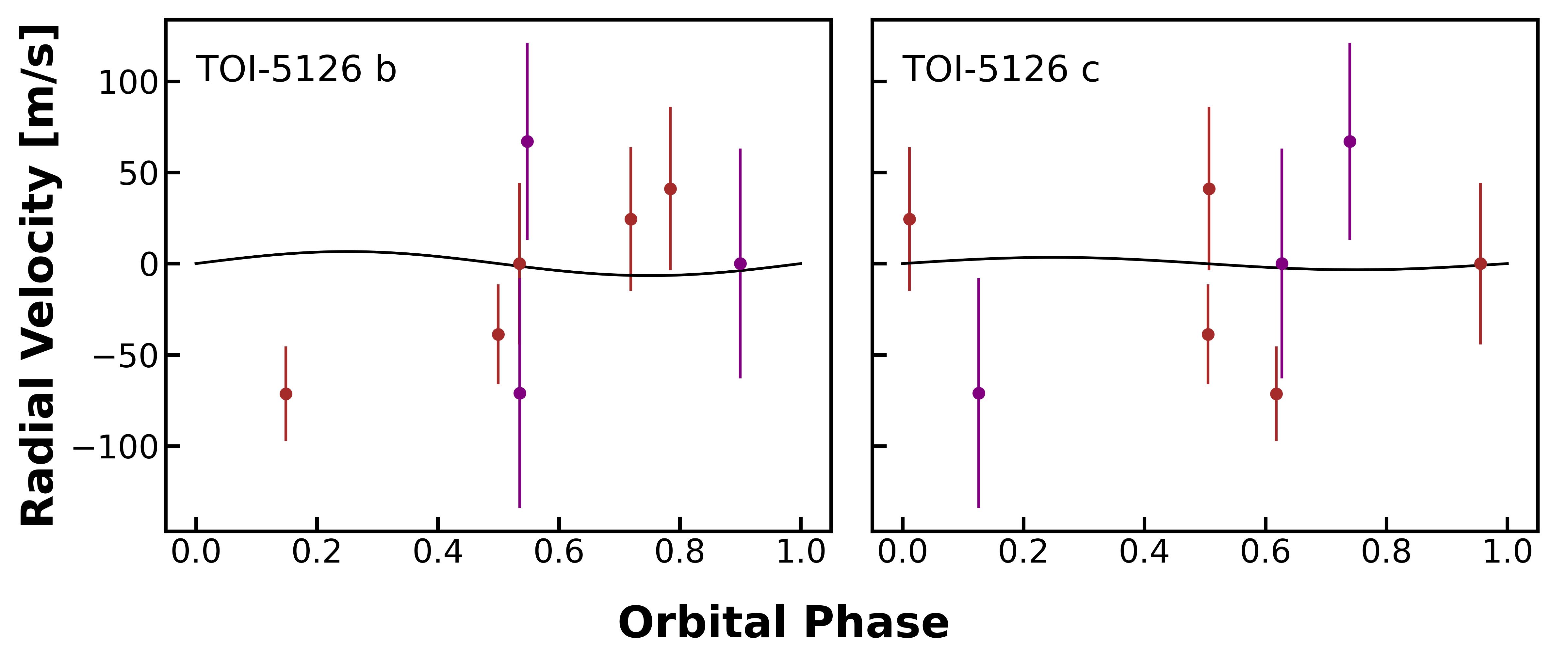
Figure 5: Left: Radial velocities against the orbital phase of TOI-5126 b with the notional K semi-amplitude curve based off of predicted mass in Section 4.5. TRES points are represented by purple points, while CHIRON data is in brown. Right: Radial velocities versus orbital phase for TOI-5126 c. with notional K semi-amplitude curve drawn from predicted mass.

Table 3: SG2 Reconnaissance Spectroscopy

Telescope	Instrument	Date (UT)	SNR	BJD	RV (kms-1)	$\sigma_{RV}$
FLWO (1.5 m)	TRES	2022-03-04	40	2459642.86967	0.000a	0.063
FLWO (1.5 m)	TRES	2022-03-13	40	2459651.79751	-0.071a	0.063
FLWO (1.5 m)	TRES	2022-03-24	40	2459662.78279	0.067a	0.054
CTIO (1.5 m)	CHIRON	2022-03-02	200	2459640.68363	11.074	0.041
CTIO (1.5 m)	CHIRON	2022-03-20	200	2459658.61297	11.154	0.050
CTIO (1.5 m)	CHIRON	2022-03-22	210	2459660.60426	11.041	0.044
CTIO (1.5 m)	CHIRON	2022-04-15	170	2459684.54751	11.113	0.056
CTIO (1.5 m)	CHIRON	2022-04-16	180	2459685.55202	11.137	0.044

2.3 High resolution imaging

As part of our standard process for validating transiting exoplanets to assess the the possible contamination of bound or unbound companions on the derived planetary radii (Ciardi et al., 2015), we observed TOI-5126 with high-resolution near-infrared adaptive optics (AO) imaging at Palomar Observatory and in the optical with speckle imaging at WIYN and SAI. The infrared observations provide the deepest sensitivities to faint companions while the optical speckle observations provide the highest resolution imaging making the two techniques complementary. Combined with Gaia, the high resolution imaging observations find no evidence for additional stellar companions within the system.

2.3.1 Palomar 5m/PHARO

The Palomar Observatory observations were made with the PHARO instrument (Hayward et al., 2001) behind the natural guide star AO system P3K (Dekany et al., 2013) on 2022 Feb 13 UT in a standard 5-point quincunx dither pattern with steps of 5″ in the narrow-band $Br-\gamma$ filter $(\lambda_{o}=2.1686;\Delta\lambda=0.0326\leavevmode\nobreak\ \mu$m). Each dither position was observed three times, offset in position from each other by 0.5″ for a total of 15 frames; with an integration time of 5.7 seconds per frame, the total on-source time was 85.5 seconds. PHARO has a pixel scale of $0.025\arcsec$ per pixel for a total field of view of $\sim 25\arcsec$. The science frames were flat-fielded and sky-subtracted. The reduced science frames were combined into a single combined image with a final resolution of 0.97″FWHM.

To within the limits of the AO observations, no stellar companions were detected. The sensitivities of the final combined AO image were determined by injecting simulated sources azimuthally around the primary target every $20^{\circ}$ at separations of integer multiples of the central source’s FWHM (Furlan et al., 2017; Lund & Ciardi, 2020). The brightness of each injected source was scaled until standard aperture photometry detected it with $5-\sigma$ significance. The resulting brightness of the injected sources relative to TOI 5126 set the contrast limits at that injection location. The final $5-\sigma$ limit at each separation was determined from the average of all of the determined limits at that separation and the uncertainty on the limit was set by the rms dispersion of the azimuthal slices at a given radial distance. Figure 6 shows no stellar companion with a difference in magnitude ($\Delta$mag) of 5.4 at a separation $\sim$0.3″, and all companions ruled out in a contrast of $\Delta$mag of 9 from $\sim$2″ onwards. No sources are present in the field-of-view with an upper limit on the angular separation of 4″.

2.3.2 WIYN 3.5m/NESSI

Further imaging observations were made using the NN-Explore Exoplanet Stellar Speckle Imager (NESSI; Scott et al. 2018) on the WIYN 3.5 m telescope at the Kitt Peak National Observatory (KPNO) in Arizona. The observation and data reduction of NESSI can be found in Howell et al. (2011). Images were taken at 832nm on UT 2022-Apr-18. The 5-$\sigma$ sensitivity curve, imaged in Figure 6, outline a $\Delta$m of 6 from 0.96″ onwards. The inset image (1.2″ angular separation) also shows no stellar neighbours within the $\Delta$m of 6.

2.3.3 SAI 2.5m/Speckle Polarimeter

A third direct image of TOI-5126 was taken using the Speckle Polarimeter on the 2.5 m Sternberg Astronomical Institute (SAI; Safonov et al. 2017). Observations were made in the $I_{c}$ filter ($\approx 660nm-825nm$). Observations were in agreement with the prior direct imaging observations, reaching a contrast of $\Delta$m of 7 from 1″.

2.3.4 Gaia Assessment

In addition to the high resolution imaging, we have utlized Gaia to identify any wide stellar companions that may be bound members of the system. Typically, these stars are already in the TESS Input Catalog and their flux dilution to the transit has already been accounted for in the transit fits and associated derived parameters. Based upon similar parallaxes and proper motions (e.g., Mugrauer & Michel, 2020, 2021; Mugrauer et al., 2022), there are no additional widely separated companions identified by Gaia.

Additionally, the Gaia DR3 astrometry provides additional information on the possibility of inner companions that may have gone undetected by either Gaia or the high resolution imaging. The Gaia Renormalised Unit Weight Error (RUWE) is a metric, similar to a reduced $\chi^{2}$, where values that are $\lesssim 1.4$ indicate that the Gaia astrometric solution is consistent with the star being single whereas RUWE values $\gtrsim 1.4$ may indicate an astrometric excess noise, possibily caused the presence of an unseen companion (e.g., Ziegler et al., 2020). TOI-5126 has a Gaia DR3 RUWE value of 1.16 indicating that the astrometric fits are consistent with the single star model. In addition the GAIA DR3 non-single-star flag is no present for the system, implying further that this is a single star system.

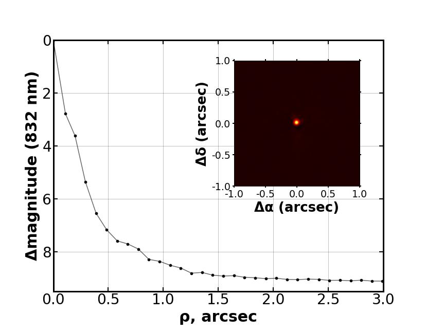
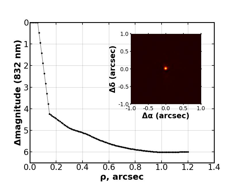
Figure 6: Left: Palomar 5.0 m companion sensitivity curve. The black points represent the 5-$\sigma$ limits. The inset image is of the primary target showing no additional close-in companions. Right: Contrast curve of TOI-5126 with the NESSI instrument on the WIYN 3.5 m telescope, reaching a constrast of $\Delta$ 6 mag from 0.96″.

3 Analysis

3.1 Stellar Parameters

Stellar parameters for TOI-5126 were obtained by fitting the star’s broadband spectral energy distribution (SED) to stellar atmosphere models using the Python package astroARIADNE (Vines & Jenkins, 2022). We used TRES spectroscopic data to define priors on the stellar effective temperature ($T_{\rm eff}$) (with its uncertainty inflated to 150 K) and metallicity (Fe/H), while distance constraints were derived from Gaia DR3 parallax (Gaia Collaboration et al., 2022). We used the default prior for Extinction ($A_{v}$) which constrains an upper limit using the SFD galactic dust maps from Schlegel et al. (1998).

astroARIADNE uses a Bayesian Model Averaging (BMA) approach, fitting multiple models accounts for model-specific systematic biases. Each model is weighed individually for a combined weighted and averaged posterior probability. This is then fed into the isochrone fitting package. In SED fitting, we used Tycho-2 (Høg et al., 2000) B and V, Gaia DR3 (Fabricius et al., 2021) G, Bp and Rp, Two-Micron All-Sky Survey (2MASS) (Skrutskie et al., 2006) J, H, K, and Wide-field Infrared Survey Explorer (WISE) (Wright et al., 2010) $W_{1}$ and $W_{2}$ bands, with an uncertainties floor applied to all bands based on Eastman et al. (2019). The weighted average results obtained are $T_{\rm eff}$ $=$ $6150_{-100}^{+130}$ K, $\log g$ $=$ $4.31_{-0.23}^{+0.24}$ cgs, $R_{\star}$ $=$ $1.249_{-0.038}^{+0.040}$  $R_{\sun}$ and [Fe/H] $=$ $0.18_{-0.13}^{+0.13}$ dex.

To identify the rotation period of TOI-5126, we passed the raw deblended SPOC light curve  through a Lomb-Scargle periodogram. The highest power of the entire TESS set of observations was constrained to be $4.602_{-0.067}^{+0.071}$ days. We used the FWHM of the highest power to derive our uncertainties. We also measured the Lomb-Scargle peaks of each sector separately, finding a scatter in the derived rotation period of $\sigma=0.066$ days, consistent with the uncertainty estimated from the peak FWHM. However, the actual uncertainty of the rotation period may be much larger and is difficult to quantify with the short observational baseline available. The periodogram can be seen in Figure 8. Given the system has a measured $v\sin I_{\star}$ of $\sim 14$ km s^-1, the inclination of the star is consistent with 90 degrees.

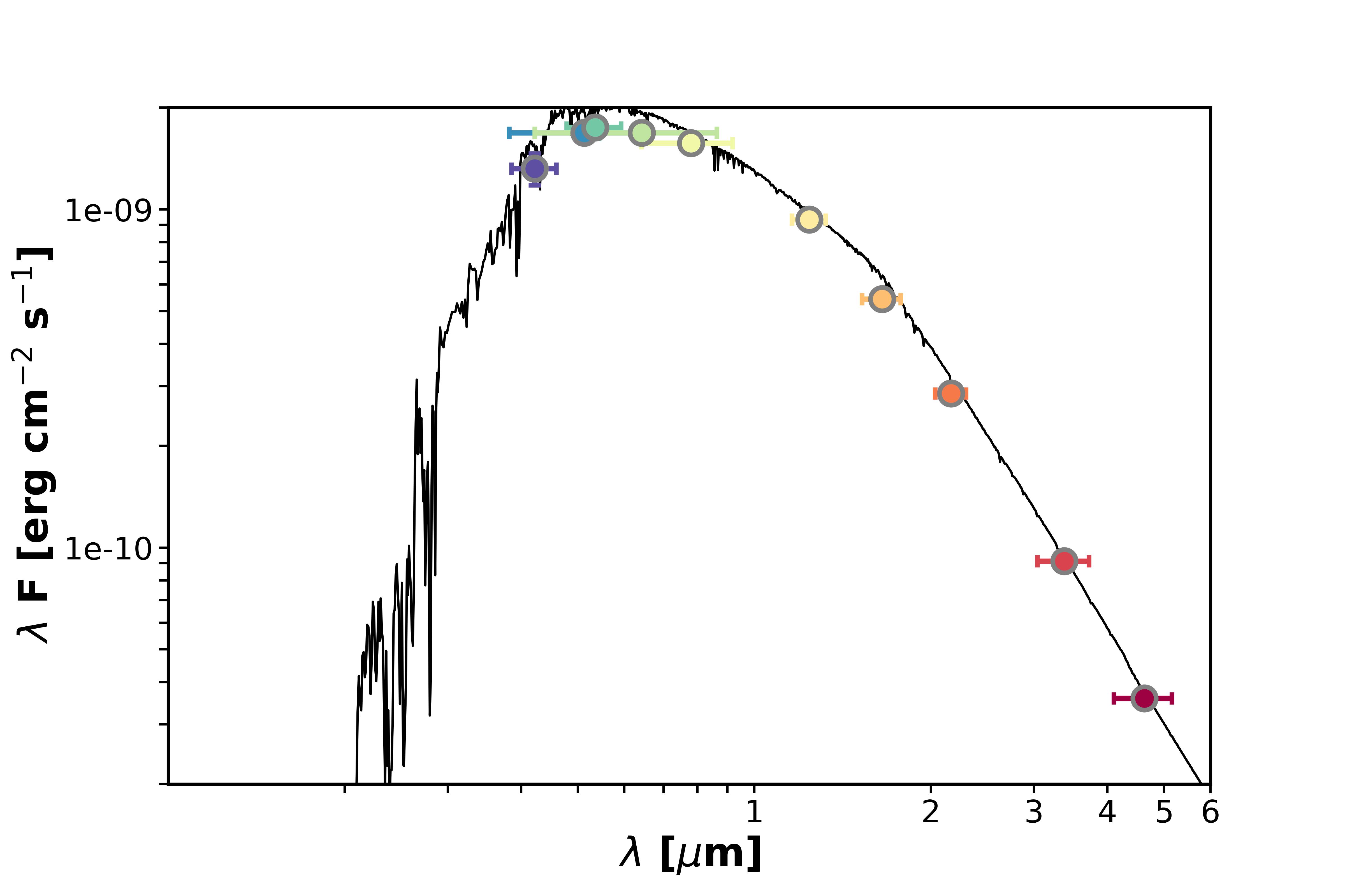
Figure 7: Spectral energy distribution (SED) of TOI-5126. Circles indicate the photometric bands with horizontal bars reflecting the passband width.

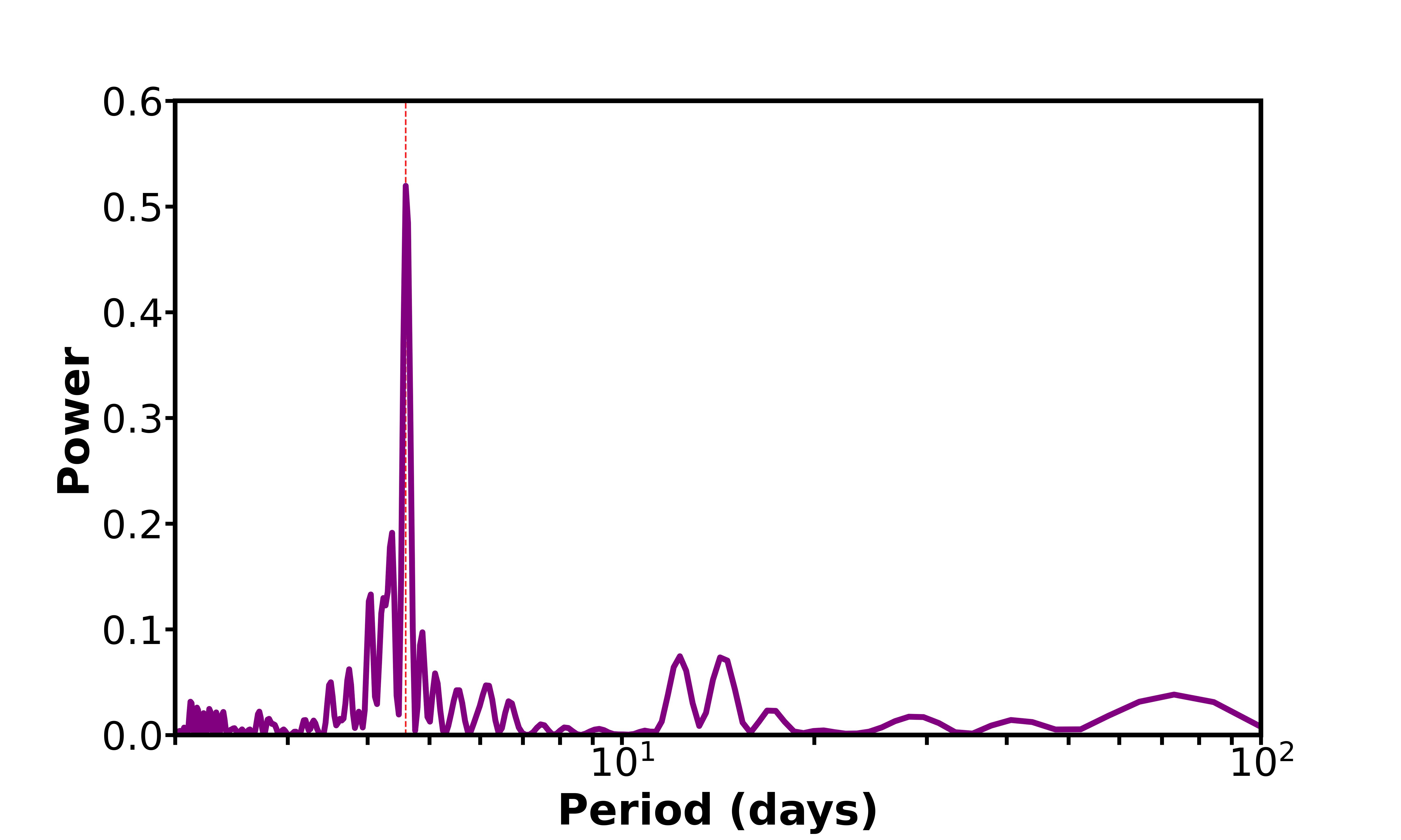
Figure 8: Lomb-Scargle periodogram of the raw SPOC TOI-5126 light curve . The highest-power period is denoted by a dashed line. Uncertainties are derived from FWHM of the highest-power resulting in a period of $4.602_{-0.067}^{+0.071}$ days.

3.2 Global Modeling

To characterise the physical parameters of the TOI-5126 system, along with their associated uncertainties, we performed a Markov Chain Monte Carlo (MCMC) fit using the publicily available software package emcee (Foreman-Mackey et al., 2013). We opted to not include the 2022-Apr-01 CTIO observation of TOI-5126 b in our fit because it only captured an ingress. Detrending was performed simultaneously to the transit fits for each photometric observation. During each iteration, we subtracted a transit model created from the batman package (Kreidberg, 2015) from the observed data. Next, we fit a trend model to the residuals using least-squares optimization, and compared the best trend model and the residuals to determine the log likelihood for the sampler. Section 2 contains further information on the individual trend models.

The global modeling process involved fitting for the two planets simultaneously. Our fit included the period, epoch, the planet-to-star radius ratio, $R_{p}$/$R_{\star}$ and impact parameter, $b$ of both planets. Eccentricities were initially fixed at 0 as we assumed a circular solution. The limb darkening coefficients for each unique photometric filter, denoted as $q_{1,i}$ and $q_{2,i}$, were included in the global fit. These coefficients were parameterised as per Kipping (2013). Additionally, we included a scaling factor for each observation as a free parameter in the fit, $c_{i}$. This accounts for differing levels of background contamination due to the varying apertures of the individual instruments. This parameter is neccessary as the large PSFs of both TESS and CHEOPS allow background stars to contribute to the measured flux, resulting in differing total fluxes to that of the LCOGT light curves . We also opted to fit for $M_{\star}$ and $R_{\star}$ to simultaneously constrain them with the planet parameters.

To constrain the period and transit times of both planets, we imposed uniform priors with boundaries at the 5-$\sigma$ upper and lower uncertainty provided by the SPOC detection pipeline. For TESS and CHEOPS, we allow the $c$ values to uniformly explore between boundaries of 0.9 to 1.1, this is due to the brightest contaminating star in TESS/CHEOPS aperture account for roughtly 5% of the light of the target star. Since the LCOGT aperture excluded all neighboring stars resolved by the Gaia catalog, we tightly constrain $c_{lco}$ to only uniformly vary between 0.99 and 1.01. For $M_{\star}$ and $R_{\star}$, we imposed a Gaussian prior derived from the results of the SED fitting obtained in Section 3.1.

We first assumed the orbits of the two planets to be circular. We also ran a set of global modeling allowing non-zero eccentricities for both planets. Our eccentric fit consisted of all previously mentioned free parameters, as well as the addition of $\sqrt{e}\cos\omega$ and $\sqrt{e}\sin\omega$ as free parameters, where $e$ is the eccentricity and $\omega$ is the longitude of periastron. These parameters could be derived to find the eccentricity and longitude of periastron of both planets. The results of both fits can be seen in Table 5.

Through visual examination of the detrended light curves  against the models, assuming a constant period, we noticed that both planets deviated slightly from their predicted transit timing assuming they are both on circular orbits. We followed the algorithm outlined in Nabbie et al. (in prep) to search for potential transit timing variations (TTVs). The 2022-Apr-01 CTIO observation of TOI-5126 b and Teid observation of TOI-5126 c were excluded due to their insufficient out-of-transit baselines. For the rest of the transits, we fit for their individual transit centers independently while allowing for the trend parameters to vary similarly to the previous model. Instead of using Gaussian priors on the stellar parameters, we added the likelihood term from the SED in our model instead so that all the stellar parameters can be constrained at the same time as the transit parameters.

For the SED likelihood, we make use of the isochrone package (Morton, 2015) and the MIST tracks. We fixed stellar parallax, distance and reddening to the best-fit values from 3.1. We added $T_{\rm eff}$, [Fe/H] and age as our free parameters, and an error scale parameter following Eastman et al. (2019). The priors of $T_{\rm eff}$ and [Fe/H] are constrained by Gaussian priors with uncertainties provided by Section 3.1. We adopt uniform priors for $M_{\star}$ and $R_{\star}$ with bounds between 1 and 1.4. The error scale was bounded between 0.01 and 100, and stellar age between 0.5 and 10 Gyr.

4 Results and Discussion

4.1 Global modeling results

Through the results of our analysis conducted in Section 3.2, we report the discovery and validation of two planets around the bright F star TOI-5126. We have determined TOI-5126 b to be a hot super-Neptune, with a radius of $4.74_{-0.14}^{+0.16}$$R_{\earth}$ in a $5.4588385_{-0.0000072}^{+0.0000070}$ day orbit. Further, we have discovered and validated TOI-5126 c as a warm Neptune at $3.86_{-0.16}^{+0.17}$$R_{\earth}$. TOI-5126 c orbits its host star every $17.8999_{-0.0013}^{+0.0018}$ days. Comparison with the current exoplanet demographic is found in Figure 12. The full parameter results are presented in Table 5. The eccentric fit and the circular fit have predominantly overlapped posterior space. We have also detected a tentative TTV signal which will be discussed in Section §4.3.3. As expected, the best fit parameters retrieved when allowing the transit times to vary in the global model, produced slightly larger transit depths and shorter transit durations for both planets. However, the joint modeling with the SED lead to a slightly smaller stellar radius. The posterior of the final planet parameters largely overlap, with the TTV fit reports TOI-5126 b having a radius of $4.67_{-0.13}^{+0.14}$$R_{\earth}$ and a transit duration of $3.686_{-0.026}^{+0.032}$ hours. For TOI-5126 c, the TTV fit reports a radius of $3.76_{-0.13}^{+0.14}$$R_{\earth}$ and a transit duration of $5.46_{-0.16}^{+0.10}$ hours.

4.2 Validation of the TOI-5126 system

Both astrophysical phenomena and instrumental artifacts can replicate the signal of a planetary transit. Without careful consideration of false positive scenarios, the legitimacy of the planet can be compromised. In this section, we validate the TOI-5126 system by ruling out false positive scenarios which could have created the observed transit signals. We consider the following scenarios:

• Either of the transit signals are a reflection of instrumental artifact: Both transit signals were detected with high significance in the TESS data, CHEOPS and ground-based telescopes as mentioned in section 2.1.3, therefore this possibility is ruled out.

• TOI-5126 is an Eclipsing Binary: This scenario is ruled out by our radial velocity observations from TRES and CHIRON (section §2.2). An analysis on the system shows that a brown dwarf companion ($M_{p}$$\approx$ 13$M_{\rm Jup}$) orbiting around TOI-5126 would produce RV semi-amplitudes of $K_{b}$= $1326$ $\rm m\,s^{-1}$ and $K_{c}$= $892$ $\rm m\,s^{-1}$. Neither sets of the radial velocity observations show such deviations.

• Light from a distant eclipsing binary or transiting planet system is blended with TOI-5126: The magnitude difference between TOI-5126 and the faintest companion which could replicate the signals observed follow as: $\Delta m\lesssim 2.5\log 10\left(\frac{t_{12}^{2}}{t_{13}^{2}\delta_{obs}}\right)$. The faintest star which could replicate the transit signals for TOI-5126 b is $\Delta$$m$ $=$ 7, and TOI-5126 c is $\Delta$$m$ $=$ 6. Direct imaging observations rule out stars with a $\Delta$$m$ of 7 from 0.5″ onwards, and ground-based photometric observations detected the transit events within a 4.7″ aperture. To statistically rule out stars within 0.5″ of TOI-5126, we determined the average stellar density in the nearby field from Gaia data. For stars within a magnitude range of seven magnitudes, the average stellar density is calculated to be $2.4\times 10^{-5}$ arcsec^-2. Narrowing this caclulation to stars six magnitudes fainter than TOI-5126, the average stellar density is $4.0\times 10^{-5}$ arcsec^-2.

An additional investigation into the probability of remaining false positive scenarios was performed using Triceratops (Giacalone & Dressing, 2020). We used the detrended TESS light curves  of TOI-5126 b and TOI-5126 c, as well as constraints provided by Palomar imaging (see section 2.3) in our analysis. A false-positive probability (FPP) of 0.77% and a nearby false-positive probability (NFPP) of 0% offer statistical validation for TOI-5126 b. Analysis of the TESS light curve  for planet c reveals a FPP and NFPP of 5.33% and 4.98%, respectively. This is invoked by a Nearby Eclipsing Binary scenario on 9.53″ away neighbour TIC27064467. This scenario, however, has been ruled out by the on-target event detected by ground-based photometry. As a result, the FPP with this scenario eliminated is 0.35%.

4.3 Dynamical constraints on the system

4.3.1 Long-term stability

The masses and eccentricities of the planets are currently not well-constrained. In this section, we explore the possibility of placing additional constraints on the system through considerations of long-term dynamical stability. We first assess the stability of the observed system using calculations of the Mean Exponential Growth factor of Nearby Orbits (MEGNO; Cincotta & Simó 2000; Cincotta et al. 2003) indicator within the REBOUND gravitational dynamics software package (Rein & Liu, 2012a). For a given set of initial conditions, we quantify the stability of the system using the time-averaged MEGNO chaos indicator value, $\langle Y(t)\rangle$, which reflects the degree of divergence of initially closely-separated trajectories in phase space. Stable system configurations will have MEGNO values $\lesssim$ 2.

The MEGNO value across a grid of different masses for both planets is displayed in the top panel of Figure 8. We are able to obtain a relatively loose constraint on the planet masses: approximately, if $M_{b}+\frac{2}{3}\,M_{c}<3M_{J}$, the system will be stable. To estimate the average MEGNO value in each cell, we randomly sample the initial condition 30 times. We assume eccentricities of both planets were randomly drawn from a Rayleigh distribution with scale parameter $0.1$. The mean anomaly and argument of periapse angles are sampled uniformly between 0 and 2 $\pi$. The integration time for each realization was set to $10^{6}$ orbits of the outermost planet with a time-step of $1/20$th of the innermost planet’s period.

We also found the system will be stable across a wide range of eccentricities for both planets if their masses approximated by the mass-radius relationship following Otegi et al. (2020). Therefore, the stability criterion alone cannot provide additional constraint on the system eccentricity.

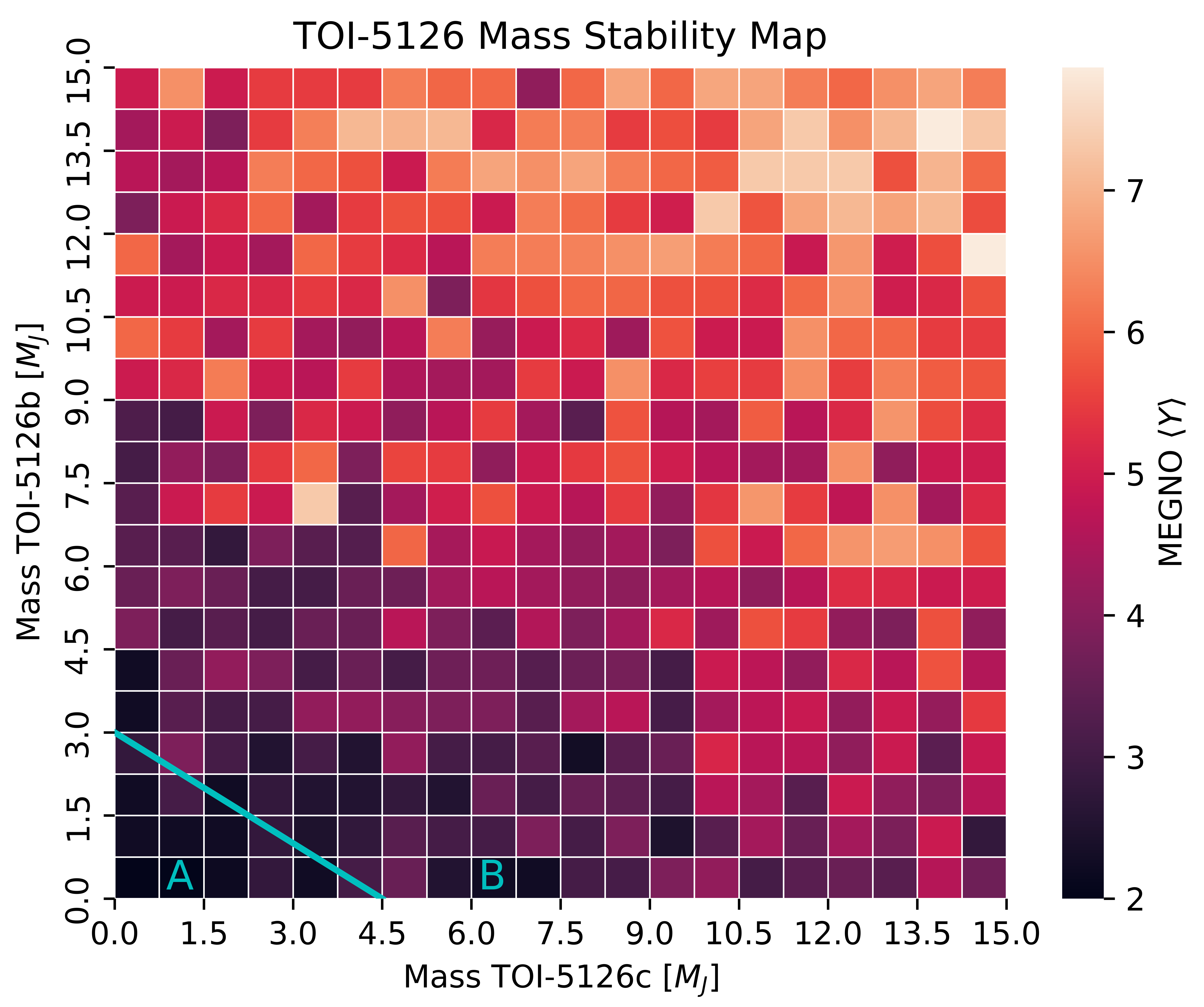
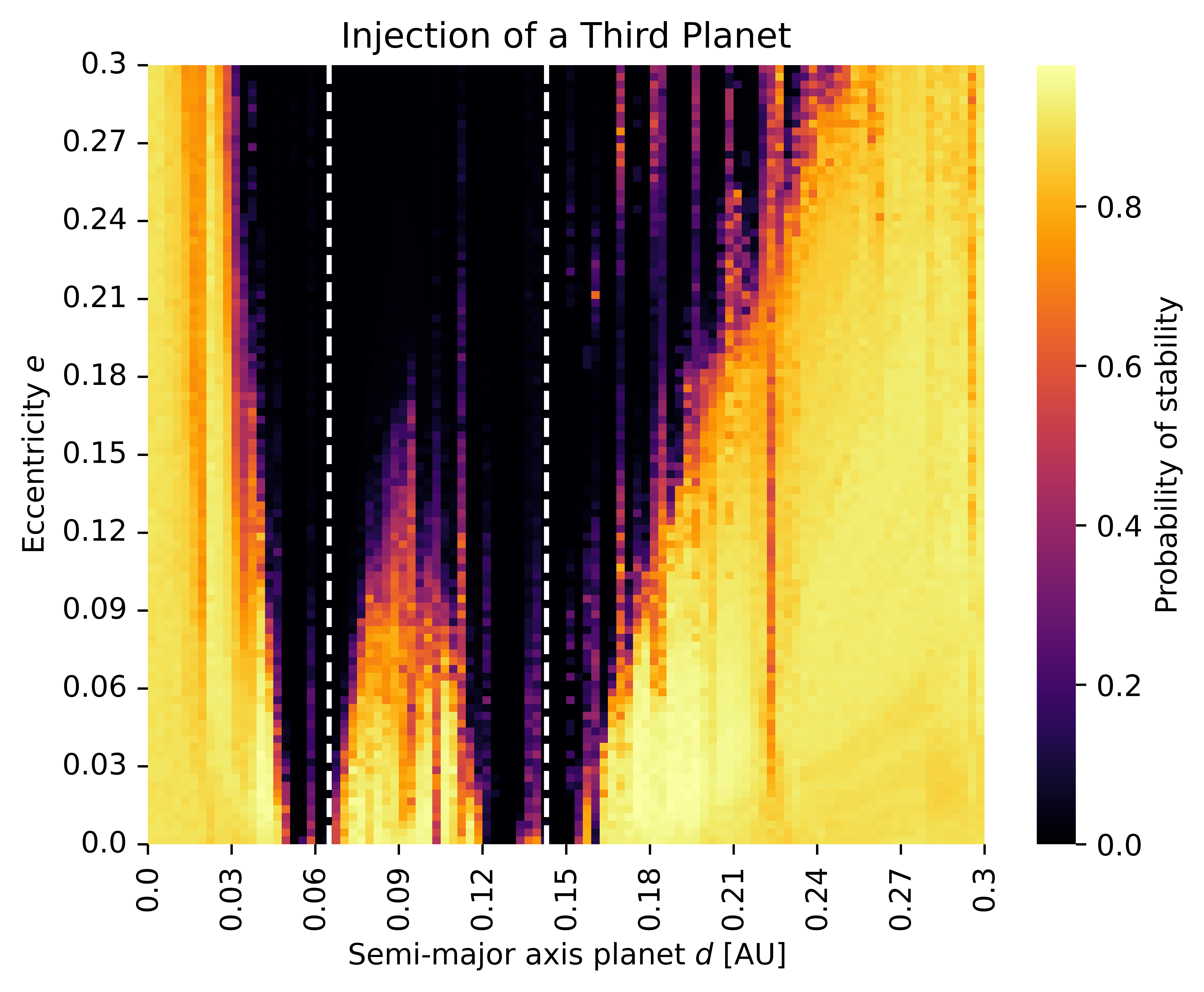
Figure 9: Top: MEGNO stability map in the $M_{b}-M_{c}$ parameter space. Two distinct regions of stability are divided by the solid cyan line, with the region A below the line indicate stable configurations. Each pixel in the $20\times 20$ map holds the average of $30$ realizations of randomized initial conditions.
Bottom: Stability map generated using SPOCK for a hypothetical third planet within the TOI-5126 system. The vertical white dashed lines denote the locations of TOI-5126 b and TOI-5126 c. Each cell in the map represents the average of 10 realizations with randomized initial conditions. There is a small stable region present between the two planets in which a hypothetical third planet could reside.

4.3.2 Stability of a hypothetical third planet

The two detected planets in the TOI-5126 system are fairly widely-spaced ($P_{c}/P_{b}\sim 3.3$). It is possible that there is a third planet residing between the orbits of the two planets or somewhere else in the system. To explore this possibility, we use the Stability of Planetary Orbital Configurations Klassifier (SPOCK; Tamayo et al. 2020) to compute the probability of stability of a given set of parameters. SPOCK is a machine learning model trained on $\sim 100,000$ orbital configurations of three-planet systems. It can estimate the probability of long-term stability of planetary systems with three or more planets.

In particular, we explored the $a_{d}-e_{d}$ space of the additional planet, whose mass we set to the average of the nominal masses of planets b and c based on the mass-radius relationship discussed in Section 4.3.1. We assumed circular orbits for planets b and c while varying the eccentricity of planet d from $0-0.3$ and semi-major axis from $0-0.3$ AU. Setting the orbits of the known planets to circular provides us with the maximum possible stable region for the hypothetical third planet. Each grid cell in the $a_{d}-e_{d}$ map represents the average of 10 realizations of the system with randomized initial conditions. Specifically, the mean anomalies, longitudes of ascending nodes, and inclinations were randomly drawn according to $M,\omega\sim\mathrm{Unif}[0,2\pi]$, $i\sim\mathrm{Rayleigh}(1^{\circ})$.

The bottom panel of Figure 9 shows the results of the SPOCK stability map for a hypothetical third planet. In addition to stable regions interior to TOI-5126 b and exterior to TOI-5126 c, there is also a stable region between the two planets. It is possible that a planet may be transiting but remain undetected due to its small radius. Alternatively, the planet could be also be either non-transiting or in the trivial case not exist at all. Nevertheless, Figure 9 indicates the ideal orbital proximity in which to search for additional planets in the system.

4.3.3 Transit timing variations signal in the light curves

From our analysis of the TESS light curves , we find that both planets exhibit tentative TTVs, seen in Figure 10. Such signals can potentially arise due to the gravitational perturbations that the planets impart on one another as they reach conjunction, creating non-periodic transit times. Notably, TOI-5126 b and TOI-5126 c are not near a first-order mean-motion resonance (MMR), which would produce the largest TTV amplitudes (Agol et al., 2005).

We utilised REBOUND (Rein & Liu, 2012a) to estimate expected TTV signals based on TOI-5126 b and TOI-5126 c alone. We sample the initial orbital elements of both planets ($a$, $e$, $w$, $i$) from the posterior distribution results from our global models (including the TTV fit) in Section 3. The other orbit angles are sampled uniformly between 0 and 2 $\pi$. The systems are integrated for more than 500 days and transit times corresponding to the observed transits from TESS, LCO and CHEOPS are recorded. The expected TTV scatter is then computed by calculating the standard deviation of the transit times after subtracting the best fit linear ephemeris. We simulated the system for 10000 realisations and found that TOI-5126 b produced 2-$\sigma$ upper limit variations of $0.27$ minutes, with TOI-5126 c exhibiting $0.19$ minute 2-$\sigma$ upper limit TTVs. The current system is therefore unable to explain the observed TTVs and we consider alternate scenarios.

One possible interpretation is that these signals imply the existence of a third, non-transiting planet in between TOI-5126 b and TOI-5126 c (as discussed in the previous section), so that one of the neighboring planet pairs have a period ratio just wide of a 3:2 resonance and the other just wide of a 2:1 resonance, both of these period ratios being commonly found in multi-planet systems (Fabrycky et al., 2014).

However, we caution that it has been shown in previous studies that spot crossing events can mimic TTV signals rather than gravitational interactions due to planets (Sanchis-Ojeda et al., 2011; Fabrycky et al., 2012; Szabó et al., 2013; Mazeh et al., 2013), especially when the individual transit has relatively low signal-to-noise. Ioannidis et al. (2016) demonstrated that a SNR larger than 15 is required to statistically minimizes the probability that a spot crossing event being the cause of the deviations. The SNR of planet b in TESS data is 13, with planet c having a SNR of 11. Given two out of three of our CHEOPS observations does not cover either ingress or egress of the transits, further high signal-to-noise photometry follow up is needed to unlock the full system architecture of TOI-5126.

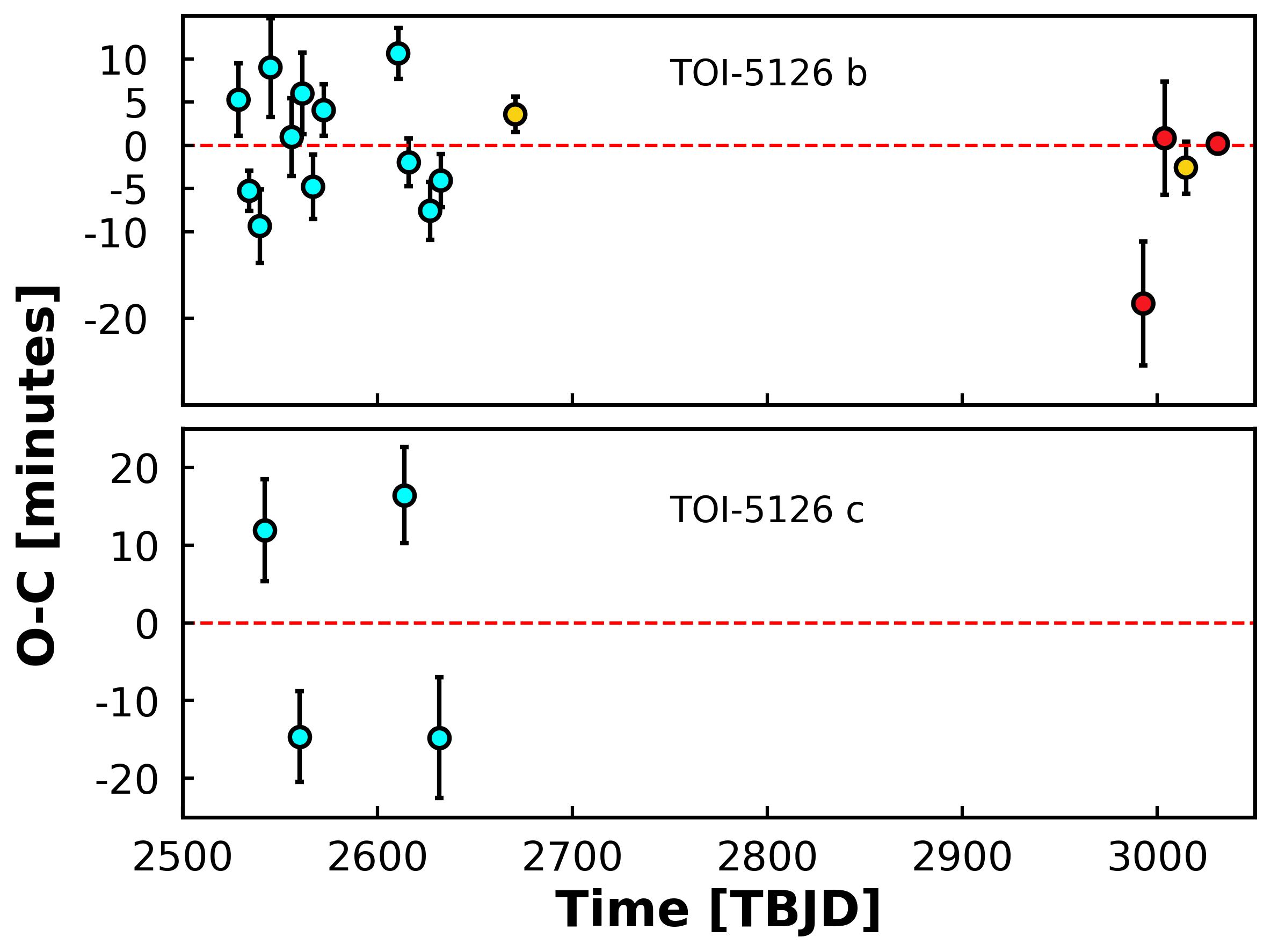
Figure 10: Transit times subtracted from a linear ephemeris for TOI-5126 b and TOI-5126 c. Cyan indicates TESS transits, yellow indicates LCOGT transits and red indicates CHEOPS transits. The red dashed line shows the expected transit time assuming a constant period.

4.4 TOI-5126 b in context with the Super-Neptune Population

TOI-5126 b is the newest addition to the super-Neptune population, the class of planets with radii between 4 and 8 $R_{\earth}$, and diverse compositions (with mass ranging between 6-135 $M_{\earth}$ Akeson et al. 2013). TOI-5126 b’s planetary parameters ($R_{b}$$\approx$ $4.7$ $R_{\earth}$, $P_{b}\approx$ $5.46$ days) place it in the sparsely populated $\lesssim$10 day, 4-8 $R_{\earth}$ region of the period-radius plane, known as the ‘hot Neptune desert’ (Mazeh et al., 2016) (see Figure 12)

The unusually large radius of TOI-5126 b implies that long-term mass-loss processes are likely still ongoing and may be readily observable. Of all super-Neptunes in the desert, TOI-5126 b is on an exclusive list of three (WASP-166 b, Hellier et al. 2019; LTT 9779b, Jenkins et al. 2020b) with visual magnitudes $\lesssim$10 and predicted equilibrium temperatures above the cloud-free threshold ($\gtrsim$1200 K). This makes it one of the most readily characterisable highly irradiated super-Neptune’s for transmission spectroscopic observations, where mass-loss mechanisms can be directly probed. Questions surrounding mass-loss are particularly unique for TOI-5126 as planet b is larger than planet c, despite receiving more stellar irradiation. This is in contrast to the expected outcome of photoevaporation, which implies that the inner companion would be smaller if the insolation ratio is larger. An example of the radius and insolation ratio relation, as well as the expected outcome of photoevaporation, can be seen in Figure 11.

4.5 Other future follow up opportunities

We compute predicted masses for TOI-5126 b and c based on the mass-radius relationship from Otegi et al. (2020). These predicted masses are adopted for the discussions below. The predicted masses for TOI-5126 b and c are $21_{-7}^{+9}{}$ $M_{\earth}$ and $18_{-6}^{+8}{}$ $M_{\earth}$, respectively.

The estimated RV semi-amplitudes for planets b and c are $K_{b}$ $=$ $6.6_{-2.5}^{+2.5}$ $\rm m\,s^{-1}$ and $K_{c}$ $=$ $3.8_{-1.5}^{+1.5}$ $\rm m\,s^{-1}$, respectively. Measuring the masses of both planets are important to determine if they are formed with large protoplanetary cores and therefore a large gaseous envelope (Lee & Chiang, 2016b) or inflated atmosphere due to tidal heating (Millholland et al., 2020). TOI-5126’s high rotational velocity makes RV measurements difficult, but with the next generation of instruments such as MAROON-X (Seifahrt et al., 2018), along with innovative methods to correct for stellar variability, mass constraints of both planets are not ruled out. The rapid rotation of TOI-5126 does however enable follow-up studies into the spin-orbit alignment of the system with the Rossiter-McLaughlin effect (R-M, Rossiter 1924; McLaughlin 1924). TOI-5126 b has a predicted R-M semi-amplitude $K_{b}$ $=$ ${11.70}_{-0.45}^{+0.41}$ $\rm m\,s^{-1}$, and planet c $K_{c}$ $=$ ${7.52}_{-0.41}^{+0.43}$ $\rm m\,s^{-1}$.

The planets in the TOI-5126 system present an ideal opportunity to better understand the atmospheric composition difference between a hot super-Neptune and a warm Neptune. TOI-5126 b still likely retains a significant H/He atmosphere due to its inflated radius.

TOI-5126 is relatively bright, with a $J$ band magnitude of 9.04. The inner planet TOI-5126 b has an equilibrium temperature of ($T_{\rm eq}$$=$ ${1442}_{-40}^{+46}$ K), and should host a relatively clear atmosphere. To test its suitability for follow-up, we followed the transmission spectroscopy metric (TSM; Kempton et al. 2018) and find that TOI-5126 b has a TSM of $84_{-25}^{+53}$. Given the potential of TOI-5126 c to also be a candidate for transmission spectroscopy (TSM $=$ $40_{-12}^{+27}$), this system enables the potential of atmospheric comparative planetology studies between a hot super-Neptune and warm Neptune. The suitability of the TOI-5126 planets for follow-up studies can be seen in comparison to the super-Neptune population in Figure 13, where despite TOI-5126 c being a Neptune, its high insolation flux ($S_{c}$ = $96_{-8}^{+9}$ $S_{\earth}$) and predicted equilibrium temperature ($T_{\rm eq}$ = $971_{-27}^{+31}$ K) make it favourable even among super-Neptunes.

To demonstrate the possibility of comparative studies, we conducted preliminary atmospheric simulations using the public software package petitRADTRANS (Mollière et al., 2019). As we are focused on identifying differences in the M/H and C/O ratios of the two planets, we used the NIRSpec Bright Object Time Series (BOTS) template with a G395H grating for our simulations. We first simulated varying M/H, including 1x, 10x and 100x Solar. We also simulate the different C/O ratios at 0.2, 0.53 (Solar) and 1.0 C/O levels, in this case assuming 10x solar M/H. The results can be seen in Figure 14.

The key features of the G395H grating are the $\mathrm{CH_{4}}$ and $\mathrm{CO_{2}}$ features in the spectra where both planets can be probed to compare formation theories. In this case, a high C/O ratio and metallicity would imply formation in a gas-depleted disk, while low C/O ratios for the planets would support other formation mechanisms. We show that differing $\mathrm{CO_{2}}$ abundances can be discerned in both TOI-5126 b and TOI-5126 c in the M/H simulation, while TOI-5126 c appears to also have a small $\mathrm{CH_{4}}$ feature at lower metallicities due to its lower predicted equilibrium temperature. The varying C/O models show that if TOI-5126 c has a high $\mathrm{CH_{4}}$ abundance, its chemical signature will be apparent in the spectrum, while lower levels would as a result produce a larger $\mathrm{CO_{2}}$ bump. The high equilibrium temperature of TOI-5126 b diminishes the signature of the $\mathrm{CH_{4}}$ feature at high C/O ratios.

Figure 11: Radius ratios of all known inner/outer planet pairs as a function of their insolation ratios. The colours represent the inner planets’ insolation flux in Earth units. The horizontal dashed line at one represents a same sized planet pair, with the arrow outlining the decrease in radius ratio expected by photoevaporation of the inner hotter planet. This plot makes use of data from the NASA exoplanet archive (Akeson et al., 2013) downloaded on 2023-02-07 UT. The data extracted only planets with measured periods, radii and host star masses, radii and effective temperatures known.

Figure 12: Radius relative to insolation flux for the population of confirmed planets. Colours represent the host star effective temperature. Plots were made with data downloaded from NASA exoplanet archive on 2023-02-07 UT.

Figure 13: TOI-5126 planets among all super-Neptunes in terms of orbital period and Transmission Spectroscopy Metric (TSM). TOI-5126 c is notably not a super-Neptune and is outlined for comparative purposes as a dashed line. The color of each point describes the planets’ insolation flux, with point size representing their scaled radius. This plot makes use of data from the NASA exoplanet archive downloaded on 2023-02-07 UT.

Figure 14: Simulated JWST Transmission Spectrums of both planets with varying metallicities and C/O ratios. Left: The red, blue and brown lines represent the varied models of 1x, 10x and 100x Solar M/H respectively. Right: C/O simulations were based off a 10x M/H baseline. the purple, light blue and brown lines indicate 0.2, 0.53 (Solar) and 1.0 C/O ratios.

5 Data Availability

All RV measurements used in our joint model analysis have been included in this paper’s tables. The TESS data products from which we derived our light curves are publicly available online from the Mikulski Archive for Space Telescopes (MAST). Ground-based observations used in this paper is available from ExoFOP-TESS. CHEOPS data will be shared on reasonable request to the lead author.

Table 4: Stellar Parameters for TOI-5126

Parameter	Value	Source
Catalog Information
R.A. (h:m:s)	10:06:38.34	Gaia DR3
Dec. (d:m:s)	+18:38:02.62	Gaia DR3
Epoch	$2016.0$	Gaia DR3
Parallax (mas)	$6.224\pm 0.022$	Gaia DR3
$\mu_{ra}$ (mas yr-1)	$-54.700\pm 0.022$	Gaia DR3
$\mu_{dec}$ (mas yr-1)	$-10.4043\pm 0.016$	Gaia DR3
Gaia DR3 ID	$623633615066248576$
TIC ID	$27064468$
TOI ID	$5126$
Photometric properties
$TESS$ (mag)	$9.5622\pm 0.0064$	TIC v8.2
$Gaia$ (mag)	$9.946\pm 0.006$	Gaia DR3
Gaia RP (mag)	$9.519\pm 0.012$	Gaia DR3
Gaia BP (mag)	$10.222\pm 0.013$	Gaia DR3
$V_{J}$ (mag)	$10.141\pm 0.006$	APASS DR10
$B_{J}$ (mag)	$10.573\pm 0.108$	APASS DR10
$J$ (mag)	$9.043\pm 0.018$	2MASS
$H$ (mag)	$8.845\pm 0.015$	2MASS
$K_{s}$ (mag)	$8.777\pm 0.018$	2MASS
$W_{1}$ (mag)	$8.712\pm 0.03$	WISE
$W_{2}$ (mag)	$8.743\pm 0.03$	WISE
Derived Properties
$M_{\star}$($M_{\sun}$)	$1.240_{-0.046}^{+0.050}$	Constant Period Circular Fit
$R_{\star}$($R_{\sun}$)	$1.241_{-0.027}^{+0.032}$	Constant Period Circular Fit
$\log{g_{\star}}$ (cgs)	$4.224_{-0.062}^{+0.051}$	Constant Period Circular Fit
$L_{\star}$ ($L_{\sun}$)	$1.99_{-0.17}^{+0.18}$	Constant Period Circular Fit
$T_{\rm eff\star}$ (K)	$6150_{-130}^{+110}$	SED
$[Fe/H]$ (dex)	$0.18_{-0.13}^{+0.13}$	SED
Distance (pc)	$161.1\pm 1.2$	SED
$\rho_{\star}$($\rm g\,cm^{-3}$)	$0.922_{-0.079}^{+0.065}$	Constant Period Circular Fit
Age (Gyr)	$0.8_{-0.7}^{+2.8}$	SED
Limb-darkening coefficients
$u_{\mathrm{1,TESS}}$	$0.25_{-0.17}^{+0.17}$
$u_{\mathrm{2,TESS}}$	$0.34_{-0.19}^{+0.25}$
$u_{\mathrm{1,z_{s}}}$	$0.56_{-0.39}^{+0.33}$
$u_{\mathrm{2,z_{s}}}$	$0.26_{-0.39}^{+0.33}$
$u_{\mathrm{2,CHEOPS}}$	$0.09_{-0.21}^{+0.29}$
$u_{\mathrm{2,CHEOPS}}$	$0.09_{-0.21}^{+0.29}$
Scaling coefficients
$c_{\mathrm{TESS}}$	$1.056_{-0.045}^{+0.023}$
$c_{\mathrm{McD}}$	$1.0001_{-0.0063}^{+0.0070}$
$c_{\mathrm{Teid}}$	$0.9986_{-0.0060}^{+0.0075}$
$c_{\mathrm{CTIO,1}}$	$0.998_{-0.005}^{+0.010}$
$c_{\mathrm{CTIO,2}}$	$0.9963_{-0.0044}^{+0.0084}$
$c_{\mathrm{CHEOPS,1}}$	$1.075_{-0.040}^{+0.017}$
$c_{\mathrm{CHEOPS,2}}$	$1.011_{-0.035}^{+0.052}$
$c_{\mathrm{CHEOPS,3}}$	$1.064_{-0.036}^{+0.025}$

Table 5: Planet Parameters for TOI-5126

Parameter	Constant Period
	Circular		Eccentric
	TOI-5126 b	TOI-5126 c	TOI-5126 b	TOI-5126 c
Light curve parameters
$P$ (days)	$5.4588385_{-0.0000072}^{+0.0000070}$	$17.8999_{-0.0013}^{+0.0018}$	$5.4588382_{-0.0000070}^{+0.0000070}$	$17.8999_{-0.0012}^{+0.0020}$
$T_{c}$ (${\rm BJD}-2457000$)	$2627.03862_{-0.00039}^{+0.00043}$	$2613.7443_{-0.0029}^{+0.0049}$	$2627.03862_{-0.00045}^{+0.00049}$	$2613.7440_{-0.0023}^{+0.0051}$
$T_{14}$ (hr)	$3.726_{-0.016}^{+0.017}$	$5.34_{-0.17}^{+0.14}$	$3.72_{-0.17}^{+0.14}$	$5.25_{-0.57}^{+0.34}$
$T_{12}=T_{34}$ (min)	$8.00_{-0.44}^{+0.54}$	$9.97_{-0.71}^{+0.85}$	$8.08_{-0.40}^{+0.62}$	$10.3_{-1.0}^{+2.5}$
$a/R_{\star}$	$11.32_{-0.33}^{+0.26}$	$24.99_{-0.74}^{+0.57}$	$11.26_{-0.36}^{+0.33}$	$24.85_{-0.79}^{+0.73}$
$R_{p}/R_{\star}$	$0.03498_{-0.00060}^{+0.00065}$	$0.02854_{-0.00090}^{+0.00080}$	$0.03511_{-0.00058}^{+0.00063}$	$0.0287_{-0.0010}^{+0.0016}$
$b\equiv a\cos i/R_{\star}$	$0.24_{-0.14}^{+0.10}$	$0.34_{-0.14}^{+0.10}$	$0.24_{-0.14}^{+0.15}$	$0.38_{-0.23}^{+0.20}$
$i$ (deg)	$88.79_{-0.53}^{+0.72}$	$89.23_{-0.25}^{+0.32}$	$88.82_{-0.82}^{+0.69}$	$89.13_{-0.49}^{+0.53}$
$e$	0 (Fixed)	0 (Fixed)	$0.09_{-0.07}^{+0.21}$	$0.21_{-0.16}^{+0.40}$
$\omega$ (deg)	0 (Fixed)	0 (Fixed)	$-10_{-130}^{+110}$	$-20_{-120}^{+130}$
Planetary parameters
$R_{p}$ ($R_{\earth}$)	$4.74_{-0.14}^{+0.16}$	$3.86_{-0.16}^{+0.17}$	$4.76_{-0.15}^{+0.17}$	$3.90_{-0.18}^{+0.26}$
$a$ (AU)	$0.06519_{-0.00082}^{+0.00087}$	$0.1439_{-0.0018}^{+0.0019}$	$0.0650_{-0.0009}^{+0.0011}$	$0.1435_{-0.0020}^{+0.0025}$
$T_{\rm eq}$ (K)	${1442}_{-40}^{+46}$	$971_{-27}^{+31}$	$1445_{-46}^{+52}$	$972_{-31}^{+35}$
$\langle F\rangle$ ($S_{\earth}$)	$467_{-39}^{+44}$	$96_{-8}^{+9}$	$471_{-44}^{+48}$	$97_{-9}^{+10}$

¹ University of Southern Queensland, West St, Darling Heights, Toowoomba, Queensland, 4350, Australia
²Department of Physics and Kavli Institute for Astrophysics and Space Research, Massachusetts Institute of Technology, 77 Massachusetts Ave, Cambridge, MA 02139, USA
³ Sternberg Astronomical Institute Lomonosov Moscow State University 119992, Moscow, Russia, Universitetskii prospekt, 13
⁴ Center for Astrophysics | Harvard & Smithsonian, 60 Garden Street, Cambridge, MA 02138, USA
⁵ NASA Exoplanet Science Institute - Caltech/IPAC, 1200 E. California Blvd, Pasadena, CA 91125 USA
⁶ George Mason University, 4400 University Drive, Fairfax, VA, 22030 USA
⁷ NSF’s National Optical-Infrared Astronomy Research Laboratory, 950 N. Cherry Avenue, Tucson, AZ 85719, USA
⁸ NASA Ames Research Center, Moffett Field, CA 94035, USA
⁹ Instituto de Astrofísica de Canarias (IAC), E-38205 La Laguna, Tenerife, Spain
¹⁰ Departamento de Astrofísica, Universidad de La Laguna (ULL), E-38206 La Laguna, Tenerife, Spain
¹² Kotizarovci Observatory, Sarsoni 90, 51216 Viskovo, Croatia
¹³ Department of Earth, Atmospheric, and Planetary Sciences, Massachusetts Institute of Technology, Cambridge, MA 02139, USA
¹⁴ Department of Aeronautics and Astronautics, Massachusetts Institute of Technology, Cambridge, MA 02139, USA
¹⁵ Department of Astrophysical Sciences, Princeton University, Princeton, NJ 08544, USA
¹⁶ Department of Astronomy, MC 249-17, California Institute of Technology, Pasadena, CA 91125, USA
¹⁷ Department of Physics and Astronomy, University of New Mexico, 210 Yale Blvd NE, Albuquerque, NM 87106, USA
¹⁸ Center for Computational Astrophysics, Flatiron Institute, 162 5th Ave New York, NY 10010, USA

References

- Agol et al. (2005) Agol E., Steffen J., Sari R., Clarkson W., 2005, MNRAS, 359, 567
- Akeson et al. (2013) Akeson R. L., et al., 2013, Publications of the Astronomical Society of the Pacific, 125, 989
- Allard et al. (2012) Allard F., Homeier D., Freytag B., 2012, Philosophical Transactions of the Royal Society of London Series A, 370, 2765
- Armstrong et al. (2020) Armstrong D. J., et al., 2020, Nature, 583, 39
- Astropy Collaboration et al. (2018) Astropy Collaboration et al., 2018, The Astronomical Journal, 156, 123
- Benz et al. (2021) Benz W., et al., 2021, Experimental Astronomy, 51, 109
- Borucki et al. (2010) Borucki W. J., et al., 2010, Science, 327, 977
- Brown et al. (2013) Brown T. M., et al., 2013, Publications of the Astronomical Society of the Pacific, 125, 1031
- Buchhave et al. (2010) Buchhave L. A., et al., 2010, ApJ, 720, 1118
- Ciardi et al. (2015) Ciardi D. R., Beichman C. A., Horch E. P., Howell S. B., 2015, ApJ, 805, 16
- Cincotta & Simó (2000) Cincotta P. M., Simó C., 2000, A&AS, 147, 205
- Cincotta et al. (2003) Cincotta P. M., Giordano C. M., Simó C., 2003, Physica D Nonlinear Phenomena, 182, 151
- Collins et al. (2017) Collins K. A., Kielkopf J. F., Stassun K. G., Hessman F. V., 2017, AJ, 153, 77
- Crossfield et al. (2020) Crossfield I. J. M., et al., 2020, ApJ, 903, L7
- Czesla et al. (2019) Czesla S., Schröter S., Schneider C. P., Huber K. F., Pfeifer F., Andreasen D. T., Zechmeister M., 2019, PyA: Python astronomy-related packages (ascl:1906.010)
- Dekany et al. (2013) Dekany R., et al., 2013, ApJ, 776, 130
- Eastman et al. (2019) Eastman J. D., et al., 2019, arXiv e-prints, arXiv:1907.09480
- Eisner et al. (2020) Eisner N. L., et al., 2020, MNRAS, 494, 750
- Fűrész et al. (2008) Fűrész G., Szentgyorgyi A. H., Meibom S., 2008, in Santos N. C., Pasquini L., Correia A. C. M., Romaniello M., eds, Precision Spectroscopy in Astrophysics. pp 287–290, doi:10.1007/978-3-540-75485-5_68
- Fabricius et al. (2021) Fabricius C., et al., 2021, Astronomy and Astrophysics, 649, A5
- Fabrycky et al. (2012) Fabrycky D. C., et al., 2012, ApJ, 750, 114
- Fabrycky et al. (2014) Fabrycky D. C., et al., 2014, ApJ, 790, 146
- Foreman-Mackey et al. (2013) Foreman-Mackey D., Hogg D. W., Lang D., Goodman J., 2013, PASP, 125, 306
- Fortney et al. (2007) Fortney J. J., Marley M. S., Barnes J. W., 2007, ApJ, 659, 1661
- Furlan et al. (2017) Furlan E., et al., 2017, AJ, 153, 71
- Gaia Collaboration et al. (2022) Gaia Collaboration et al., 2022, Gaia Data Release 3: Summary of the Content and Survey Properties
- Giacalone & Dressing (2020) Giacalone S., Dressing C. D., 2020, Astrophysics Source Code Library, p. ascl:2002.004
- Gillon et al. (2007) Gillon M., et al., 2007, A&A, 472, L13
- Guerrero et al. (2021) Guerrero N. M., et al., 2021, The Astrophysical Journal Supplement Series, 254, 39
- Harris et al. (2020) Harris C. R., et al., 2020, Nature, 585, 357
- Hauschildt et al. (1999) Hauschildt P. H., Allard F., Ferguson J., Baron E., Alexander D. R., 1999, ApJ, 525, 871
- Hayward et al. (2001) Hayward T. L., Brandl B., Pirger B., Blacken C., Gull G. E., Schoenwald J., Houck J. R., 2001, PASP, 113, 105
- Hellier et al. (2019) Hellier C., et al., 2019, Monthly Notices of the Royal Astronomical Society, 488, 3067
- Høg et al. (2000) Høg E., et al., 2000, A&A, 355, L27
- Howell et al. (2011) Howell S. B., Everett M. E., Sherry W., Horch E., Ciardi D. R., 2011, AJ, 142, 19
- Howell et al. (2014) Howell S. B., et al., 2014, PASP, 126, 398
- Hoyer et al. (2020) Hoyer S., Guterman P., Demangeon O., Sousa S. G., Deleuil M., Meunier J. C., Benz W., 2020, A&A, 635, A24
- Huang et al. (2020) Huang C. X., et al., 2020, arXiv:2011.06459 [astro-ph 10.17909/t9-r086-e880
- Hunter (2007) Hunter J. D., 2007, Computing in Science and Engineering, 9, 90
- Husser et al. (2013) Husser T.-O., Wende von Berg S., Dreizler S., Homeier D., Reiners A., Barman T., Hauschildt P., 2013, Astronomy and Astrophysics, 553
- Ioannidis et al. (2016) Ioannidis P., Huber K. F., Schmitt J. H. M. M., 2016, A&A, 585, A72
- Jenkins et al. (2002) Jenkins J. M., Caldwell D. A., Borucki W. J., 2002, ApJ, 564, 495
- Jenkins et al. (2010) Jenkins J. M., et al., 2010, in Radziwill N. M., Bridger A., eds, Society of Photo-Optical Instrumentation Engineers (SPIE) Conference Series Vol. 7740, Software and Cyberinfrastructure for Astronomy. p. 77400D, doi:10.1117/12.856764
- Jenkins et al. (2016) Jenkins J. M., et al., 2016, in Chiozzi G., Guzman J. C., eds, Society of Photo-Optical Instrumentation Engineers (SPIE) Conference Series Vol. 9913, Software and Cyberinfrastructure for Astronomy IV. p. 99133E, doi:10.1117/12.2233418
- Jenkins et al. (2020a) Jenkins J. S., et al., 2020a, Nature Astronomy, 4, 1148
- Jenkins et al. (2020b) Jenkins J. M., Twicken J. D., Tenenbaum P., Ting E. B., Caldwell D. A., Smith J., Rose M., Wohler B., 2020b, in AAS/Division for Planetary Sciences Meeting Abstracts. p. 207.03
- Jensen (2013) Jensen E., 2013, Tapir: A web interface for transit/eclipse observability, Astrophysics Source Code Library (ascl:1306.007)
- Jin et al. (2014) Jin S., Mordasini C., Parmentier V., van Boekel R., Henning T., Ji J., 2014, The Astrophysical Journal, 795, 65
- Kempton et al. (2018) Kempton E. M.-R., et al., 2018, Publications of the Astronomical Society of the Pacific, 130, 114401
- Kipping (2013) Kipping D. M., 2013, Monthly Notices of the Royal Astronomical Society, 435, 2152
- Kreidberg (2015) Kreidberg L., 2015, PASP, 127, 1161
- Kurucz (1993) Kurucz R. L., 1993, SYNTHE spectrum synthesis programs and line data
- Lee & Chiang (2016a) Lee E. J., Chiang E., 2016a, ApJ, 817, 90
- Lee & Chiang (2016b) Lee E. J., Chiang E., 2016b, ApJ, 817, 90
- Lee et al. (2014) Lee E. J., Chiang E., Ormel C. W., 2014, ApJ, 797, 95
- Li et al. (2019) Li J., Tenenbaum P., Twicken J. D., Burke C. J., Jenkins J. M., Quintana E. V., Rowe J. F., Seader S. E., 2019, PASP, 131, 024506
- Lopez (2017) Lopez E. D., 2017, Monthly Notices of the Royal Astronomical Society, 472, 245
- Lund & Ciardi (2020) Lund M. B., Ciardi D., 2020, in American Astronomical Society Meeting Abstracts #235. p. 249.06
- Matsakos & Königl (2016) Matsakos T., Königl A., 2016, ApJ, 820, L8
- Maxted et al. (2022) Maxted P. F. L., et al., 2022, MNRAS, 514, 77
- Mazeh et al. (2013) Mazeh T., et al., 2013, ApJS, 208, 16
- Mazeh et al. (2016) Mazeh T., Holczer T., Faigler S., 2016, A&A, 589, A75
- McCully et al. (2018) McCully C., Volgenau N. H., Harbeck D.-R., Lister T. A., Saunders E. S., Turner M. L., Siiverd R. J., Bowman M., 2018, in Proc. SPIE. p. 107070K (arXiv:1811.04163), doi:10.1117/12.2314340
- McLaughlin (1924) McLaughlin D. B., 1924, ApJ, 60, 22
- Millholland et al. (2020) Millholland S., Petigura E., Batygin K., 2020, ApJ, 897, 7
- Mollière et al. (2019) Mollière P., Wardenier J. P., van Boekel R., Henning T., Molaverdikhani K., Snellen I. A. G., 2019, A&A, 627, A67
- Morris et al. (2020) Morris R. L., Twicken J. D., Smith J. C., Clarke B. D., Jenkins J. M., Bryson S. T., Girouard F., Klaus T. C., 2020, Kepler Data Processing Handbook: Photometric Analysis, Kepler Science Document KSCI-19081-003
- Morton (2015) Morton T. D., 2015, isochrones: Stellar model grid package, Astrophysics Source Code Library, record ascl:1503.010 (ascl:1503.010)
- Mugrauer & Michel (2020) Mugrauer M., Michel K.-U., 2020, Astronomische Nachrichten, 341, 996
- Mugrauer & Michel (2021) Mugrauer M., Michel K.-U., 2021, Astronomische Nachrichten, 342, 840
- Mugrauer et al. (2022) Mugrauer M., Zander J., Michel K.-U., 2022, Astronomische Nachrichten, 343, e24017
- Otegi et al. (2020) Otegi J. F., Bouchy F., Helled R., 2020, A&A, 634, A43
- Owen & Jackson (2012) Owen J. E., Jackson A. P., 2012, MNRAS, 425, 2931
- Owen & Lai (2018) Owen J. E., Lai D., 2018, Monthly Notices of the Royal Astronomical Society, 479, 5012
- Paredes et al. (2021) Paredes L. A., Henry T. J., Quinn S. N., Gies D. R., Hinojosa-Goñi R., James H.-S., Jao W.-C., White R. J., 2021, AJ, 162, 176
- Petigura et al. (2017) Petigura E. A., et al., 2017, AJ, 153, 142
- Quinn et al. (2012) Quinn S. N., et al., 2012, ApJ, 745, 80
- Reback et al. (2020) Reback J., et al., 2020, Pandas-Dev/Pandas: Pandas 1.0.3, Zenodo, doi:10.5281/zenodo.3715232
- Rein & Liu (2012a) Rein H., Liu S. F., 2012a, A&A, 537, A128
- Rein & Liu (2012b) Rein H., Liu S. F., 2012b, A&A, 537, A128
- Ricker et al. (2015) Ricker G. R., et al., 2015, Journal of Astronomical Telescopes, Instruments, and Systems, 1, 014003
- Rossiter (1924) Rossiter R. A., 1924, ApJ, 60, 15
- Safonov et al. (2017) Safonov B. S., Lysenko P. A., Dodin A. V., 2017, Astronomy Letters, 43, 344
- Sanchis-Ojeda et al. (2011) Sanchis-Ojeda R., Winn J. N., Holman M. J., Carter J. A., Osip D. J., Fuentes C. I., 2011, ApJ, 733, 127
- Schlegel et al. (1998) Schlegel D. J., Finkbeiner D. P., Davis M., 1998, ApJ, 500, 525
- Scott et al. (2018) Scott N. J., Howell S. B., Horch E. P., Everett M. E., 2018, Publications of the Astronomical Society of the Pacific, 130, 1
- Seifahrt et al. (2018) Seifahrt A., Stürmer J., Bean J. L., Schwab C., 2018, in Evans C. J., Simard L., Takami H., eds, Society of Photo-Optical Instrumentation Engineers (SPIE) Conference Series Vol. 10702, Ground-based and Airborne Instrumentation for Astronomy VII. p. 107026D (arXiv:1805.09276), doi:10.1117/12.2312936
- Skrutskie et al. (2006) Skrutskie M. F., et al., 2006, AJ, 131, 1163
- Szabó et al. (2013) Szabó R., Szabó G. M., Dálya G., Simon A. E., Hodosán G., Kiss L. L., 2013, A&A, 553, A17
- Tamayo et al. (2020) Tamayo D., et al., 2020, Proceedings of the National Academy of Science, 117, 18194
- Tokovinin et al. (2013) Tokovinin A., Fischer D. A., Bonati M., Giguere M. J., Moore P., Schwab C., Spronck J. F. P., Szymkowiak A., 2013, PASP, 125, 1336
- Twicken et al. (2010) Twicken J. D., Clarke B. D., Bryson S. T., Tenenbaum P., Wu H., Jenkins J. M., Girouard F., Klaus T. C., 2010, in Software and Cyberinfrastructure for Astronomy. p. 774023, doi:10.1117/12.856790
- Twicken et al. (2018) Twicken J. D., et al., 2018, PASP, 130, 064502
- Vines & Jenkins (2022) Vines J. I., Jenkins J. S., 2022, MNRAS,
- Virtanen et al. (2020) Virtanen P., et al., 2020, Nature Methods, 17, 261
- Wright et al. (2010) Wright E. L., et al., 2010, AJ, 140, 1868
- Zhou et al. (2021) Zhou G., et al., 2021, AJ, 161, 2
- Ziegler et al. (2020) Ziegler C., Tokovinin A., Briceño C., Mang J., Law N., Mann A. W., 2020, AJ, 159, 19