Provably Robust Cost-Sensitive Learning via Randomized Smoothing

Abstract

We focus on learning adversarially robust classifiers under a cost-sensitive scenario, where the potential harm of different classwise adversarial transformations is encoded in a binary cost matrix. Existing methods are either empirical that cannot certify robustness or suffer from inherent scalability issues. In this work, we study whether randomized smoothing, a more scalable robustness certification framework, can be leveraged to certify cost-sensitive robustness. Built upon a notion of cost-sensitive certified radius, we show how to adapt the standard randomized smoothing certification pipeline to produce tight robustness guarantees for any cost matrix. In addition, with fine-grained certified radius optimization schemes specifically designed for different data subgroups, we propose an algorithm to train smoothed classifiers that are optimized for cost-sensitive robustness. Extensive experiments on image benchmarks and a real-world medical dataset demonstrate the superiority of our method in achieving significantly improved performance of certified cost-sensitive robustness while having a negligible impact on overall accuracy.

1 Introduction

Recent studies have revealed that deep learning models are highly vulnerable to adversarial examples. To improve model robustness in the presence of adversarial examples, various defensive mechanisms have been proposed, primarily falling into two categories: empirical defenses (Goodfellow et al., 2014; Papernot et al., 2016; Kurakin et al., 2016; Madry et al., 2017; Zhang et al., 2019) and certifiable methods (Raghunathan et al., 2018; Wong & Kolter, 2018; Gowal et al., 2018; Cohen et al., 2019; Lecuyer et al., 2019; Jia et al., 2019; Li et al., 2019). Compared with empirical defenses, certifiable methods can produce a robustness certificate for the model prediction to remain unchanged within some specific norm-bounded perturbation ball of any test input and train models to be provably robust. These methods avoid the undesirable arms race between newly-designed empirical defenses and stronger adaptive attacks that break those defenses (Carlini & Wagner, 2017; Athalye et al., 2018).

Most existing defenses aim to improve the overall robustness of a classification model, assuming the same penalty is imposed on all kinds of adversarial misclassifications. For real-world applications, however, it is likely that some specific misclassifications are more consequential than others (Domingos, 1999; Elkan, 2001). For instance, misclassifying a malignant tumor as benign in the application of medical diagnosis is much more detrimental to a patient than the reverse. Therefore, instead of solely focusing on enhancing overall robustness, the development of defenses should also account for the difference in costs induced by different adversarial examples. In line with existing works on cost-sensitive robust learning (Domingos, 1999; Asif et al., 2015; Zhang & Evans, 2019; Chen et al., 2021), we aim to develop models that are robust to cost-sensitive adversarial misclassifications, while maintaining the standard overall classification accuracy. However, existing defenses are either hindered by their foundational reliance on heuristics, which often fall short of providing a robustness guarantee (Domingos, 1999; Asif et al., 2015; Chen et al., 2021) or suffer from inherent scalability issues when certifying robustness for large models and perturbations (Zhang & Evans, 2019).

To achieve the best of both worlds, we propose to learn provably cost-sensitive robust classifiers by leveraging randomized smoothing (Liu et al., 2018; Cohen et al., 2019; Salman et al., 2019), an emerging robustness certification framework that has attracted a lot of attention due to its simplicity and scalability. However, optimizing smoothed classifiers for cost-sensitive robustness is intractable, primarily due to the inherent complexity introduced by the discrete Gaussian sampling process when transforming base classifiers into smoothed classifiers. In addition, different designs of cost matrix necessitate a more flexible and targeted optimization scheme than optimizing for overall robustness.

Contributions. We are the first to adapt the randomized smoothing framework to certify and train for cost-sensitive robustness. In particular, for any binary cost matrix (Section 2), we introduce the notion of cost-sensitive certified radius (Definition 3.1), which captures the maximum allowable $\ell_{2}$ perturbation with respect to the smoothed classifier for each sensitive seed input (Theorem 3.2). We show that compared with standard certified radius typically adopted in the literature, our proposed definition is more suitable for certifying cost-sensitive robustness, as it theoretically defines a larger certified radius specifically for a wide range of cost matrices (Theorem 3.3). Built upon the definition of cost-sensitive certified radius, we further propose a practical certification algorithm using Monte Carlo samples (Algorithm 1), which provides two different methods for computing the probabilistic bound on certified radius such that the tighter bound can always be returned (Section 3.2). In addition, to train for cost-sensitive robust smoothed classifiers, we attempt to adapt the commonly-used reweighting method in the standard cost-sensitive learning literature (Elkan, 2001; Khan et al., 2017). However, we discover that the naive reweighting scheme does not adapt well when training a smoothed classifier, owing to the indirect optimization of the base classifier and the non-optimal trade-off between sensitive and non-sensitive examples (Section 4.1). Therefore, we take the distinctive properties of different data subgroups into account and design an advanced cost-sensitive robust training method based on MACER (Zhai et al., 2020) to directly optimize the certified radius with respect to the smoothed classifier (Section 4.2). Experiments on typical image benchmarks and a real-world medical dataset illustrate the superiority of our method in achieving consistently and significantly improved certified cost-sensitive robustness while maintaining a similar performance of overall accuracy under a wide variety of cost matrix settings (Section 1).

Related Work. We review the most related lines of research in the existing literature. In particular, Cohen et al. (2019) proposed randomized smoothing, which first converts any base neural network into a smoothed classifier by injecting Gaussian noises to inputs followed by majority voting, then provides a robust certificate that can guarantee the prediction of the resulting smoothed classifier is constant within some $\ell_{2}$-norm ball for any test input. Compared with other certification methods such as formal verification (Katz et al., 2017; Tjeng et al., 2019) and convex relaxation-based approaches (Raghunathan et al., 2018; Wong & Kolter, 2018) , the biggest advantage of randomized smoothing is its scalability to large neural networks and large-scale datasets. Later on, Shafahi et al. (2019) improved the proposed training method in Cohen et al. (2019) by designing an adaptive attack on the smoothed classifier using adversarial training and first-order approximations. In addition, Zhai et al. (2020) developed a training method named MACER, which directly optimizes the certified radius of the smoothed classifier with respect to correctly-classified samples using margin-based loss and achieves better robustness and accuracy trade-off than previous methods. More recently, several works (Carlini et al., 2022; Xiao et al., 2022; Zhang et al., 2023) proposed to improve the base classifier training pipeline by adapting pretrained diffusion models to denoise the Gaussian augmented samples. Despite of a large improvement on certified robustness over prior denoising approaches (Salman et al., 2020), the reverse process of the diffusion model required by these methods typically costs a significant amount of time, thereby posing computational challenges for both training and certification under cost-sensitive scenarios.

Moreover, cost-sensitive learning (Domingos, 1999; Elkan, 2001; Khan et al., 2017) deals with situations where different misclassifications induce different costs. While most of the existing works on cost-sensitive learning considered the standard learning setting, we are aware of a couple of research works focusing on study cost-sensitive robustness (Katsumata & Takeda, 2015; Zhang & Evans, 2019; Hartnett et al., 2019; Chen et al., 2021; Gan et al., 2021; Shen et al., 2022). However, most of these works either consider simple convex learning algorithms (Katsumata & Takeda, 2015; Chen et al., 2021; Gan et al., 2021) or propose empirical solvers based on neural networks by modifying algorithms such as adversarial training to be cost-sensitive robust (Shen et al., 2022). The most relevant work to ours is Zhang & Evans (2019), which proposed a certified cost-sensitive robust training method using standard robustness certification methods based on convex relaxation. Although their method can produce a certificate on cost-sensitive robustness, it is not scalable to large neural networks or certify perturbations of larger size, particularly due to the high computational cost required for computing the certificate. In contrast to the aforementioned methods, our work provides a certifiable and more scalable cost-sensitive robust learning method based on randomized smoothing.

2 Preliminaries

Randomized Smoothing. Cohen et al. (2019) proposed a probabilistic certification framework named randomized smoothing (RS), which is based on the following construction of smoothed classifiers.

Definition 2.1.

Let $\mathcal{X}\subseteq\mathbb{R}^{d}$ be the input space and $[m]:=\{1,2,\ldots,m\}$ be the label space. For any base classifier $f_{\theta}:\mathcal{X}\rightarrow[m]$ and $\sigma>0$, the corresponding smoothed classifier $g_{\theta}$ is defined as:

$$g_{\theta}({\bm{x}})=\underset{k\in[m]}{\operatorname*{arg\,max}}~{}\mathbb{P}_{\bm{\delta}\sim{\mathcal{N}}(\mathbf{0},\sigma^{2}\mathbf{I})}\>\big{[}f_{\theta}(\bm{x}+\bm{\delta})=k\big{]},\>\forall\bm{x}\in\mathcal{X}.$$

Let $h_{\theta}:\mathcal{X}\rightarrow[0,1]^{m}$ be the function that maps any input $\bm{x}$ to the prediction probabilities of $g_{\theta}(\bm{x})$:

$$[h_{\theta}(\bm{x})]_{k}=\mathbb{P}_{\bm{\delta}\sim{\mathcal{N}}(\mathbf{0},\sigma^{2}\mathbf{I})}\>\big{[}f_{\theta}(\bm{x}+\bm{\delta})=k\big{]},\>\forall\bm{x}\in\mathcal{X}\text{ and }k\in[m].$$

The following lemma, proven in Cohen et al. (2019), characterizes the maximum allowable $\ell_{2}$-perturbation for any input $\bm{x}$ such that the prediction of $g_{\theta}$ at $\bm{x}$ remains the same within the radius.

Lemma 2.2 (Cohen et al. (2019)).

Let $\bm{x}\in\mathcal{X}$ be any input and $y\in[m]$ be its ground-truth label. If $g_{\theta}$ classifies $\bm{x}$ correctly, i.e., $y=\operatorname*{arg\,max}_{k\in[m]}\mathbb{P}_{{\bm{\delta}\sim{\mathcal{N}}(\mathbf{0},\sigma^{2}\mathbf{I})}}\big{[}f_{\theta}({\bm{x}}+\bm{\delta})=k\big{]}$, then the prediction of $g$ at ${\bm{x}}$ is both accurate and provably robust with certified $\ell_{2}$-norm radius $R(\bm{x})$, which is defined as:

$$R(\bm{x};h_{\theta})=\frac{\sigma}{2}\Big{[}\Phi^{-1}\big{(}[h_{\theta}(\bm{x})]_{y}\big{)}-\Phi^{-1}\big{(}\max_{k\neq y}\>[h_{\theta}(\bm{x})]_{k}\big{)}\Big{]},$$ (1)

where $\Phi$ is the CDF of standard Gaussian $\mathcal{N}(0,1)$ and $\Phi^{-1}$ denotes its inverse. When $h_{\theta}$ is free of context, we simply write $R(\bm{x})=R(\bm{x};h_{\theta})$.

We remark that our method is built upon this randomized smoothing framework, which is designed for $l_{2}$ perturbations. Recent studies have adapted the standard framework to certify robustness against other $\ell_{p}$-norm bounded perturbations (Mohapatra et al., 2020; Yang et al., 2020). We believe our method is applicable to those $\ell_{p}$-norms, whereas studying how to certify cost-sensitive robustness against general perturbations defined in metrics beyond $\ell_{p}$-norm would be an interesting future work.

Cost-Sensitive Robustness. We consider robust classification tasks under cost-sensitive scenarios, where the goal is to learn a classifier with both high overall accuracy and cost-sensitive robustness. Suppose $\mathbf{C}\in\{0,1\}^{m\times m}$ is a predefined cost matrix that encodes the potential harm of different classwise adversarial transformations. In particular, the most studied overall robustness corresponds to having a cost matrix, where all the entries are $1$ except for the diagonal ones. For any $j\in[m]$ and $k\in[m]$, $C_{jk}=1$ means any misclassification from seed class $j$ to target class $k$ will induce a cost, whereas $C_{jk}=0$ suggests that there is no incentive for an attacker to trick the model to misclassify inputs from class $j$ to class $k$. Therefore, the goal of cost-sensitive robust learning is to reduce the number of adversarial misclassifications that will induce a cost defined by $\mathbf{C}$. For the ease of presentation, we also introduce the following notations. For any seed class $j\in[m]$, we let $\Omega_{j}=\{k\in[m]:C_{jk}=1\}$ be the set of cost-sensitive target classes. If $\Omega_{j}$ is an empty set, then all the examples from seed class $j$ is non-sensitive. Otherwise, any class $j$ with $|\Omega_{j}|\geq 1$ is a sensitive seed class. Given a dataset $\mathcal{S}=\{(\bm{x}_{i},y_{i})\}_{i\in[n]}$, we define the set of cost-sensitive examples as $\mathcal{S}^{\text{s}}=\{(\bm{x},y)\in\mathcal{S}:|\Omega_{y}|\geq 1\}$, while the remaining examples are regarded as non-sensitive. In this work, we focus on studying the following two main categories of cost matrices conditioned on $\Omega_{y}$:

• Seedwise: For any $({\bm{x}},y)\in\mathcal{S}^{s}$, $\Omega_{y}=\{j\in[m]:j\neq y\}$ or equivalently $|\Omega_{y}|=m-1$, meaning that any possible classwise adversarial transformation for $(\bm{x},y)$ will incur a cost. In other words, $\Omega_{y}$ contains all the possible target classes with respect to $(\bm{x},y)$.

• Pairwise: For any $({\bm{x}},y)\in\mathcal{S}^{s}$, $\Omega_{y}\subsetneqq\{j\in[m]:j\neq y\}$, suggesting that $[m]\backslash{\Omega_{y}}$ includes target class other than $y$ and misclassification to any target class in $[m]\backslash{\Omega_{y}}$ is acceptable.

3 Certifying Cost-Sensitive Robustness

This section explains how to certify cost-sensitive robustness using randomized smoothing. We first introduce the formal definition of cost-sensitive certified radius and the corresponding evaluation metrics then discuss its connection to the standard certified radius (Section 3.1). Finally, based on the proposed definition, we design a practical certification algorithm using finite samples (Section 3.2).

3.1 Cost-Sensitive Certified Radius

Recall that for any example $({\bm{x}},y)\in\mathcal{S}^{\text{s}}$, only misclassifying ${\bm{x}}$ to a target class in $\Omega_{y}$ incurs a cost, whereas misclassifications to any class from $[m]\backslash{\Omega_{y}}$ is tolerable. Below, we formally define cost-sensitive certified radius, which adapts the standard certified radius to cost-sensitive scenarios:

Definition 3.1 (Cost-Sensitive Certified Radius).

Consider the same setting as in Theorem 2.2. Let $\mathbf{C}$ be an $m\times m$ cost matrix. For any example $(\bm{x},y)\in\mathcal{X}\times[m]$ where $y$ is a sensitive seed class, the cost-sensitive certified radius at $(\bm{x},y)$ with respect to $\mathbf{C}$ is defined as:

$$R_{\text{c-s}}(\bm{x};\Omega_{y},h_{\theta})=\frac{\sigma}{2}\bigg{[}\Phi^{-1}\Big{(}\max_{k\in[m]}\>\big{[}h_{\theta}(\bm{x})\big{]}_{k}\Big{)}-\Phi^{-1}\Big{(}\max_{k\in\Omega_{y}}\>\big{[}h_{\theta}(\bm{x})\big{]}_{k}\Big{)}\bigg{]},$$

where $\Omega_{y}=\{k\in[m]:C_{yk}=1\}$, and $\Phi^{-1}$ is the inverse CDF of standard Gaussian $\mathcal{N}(0,1)$. When $h_{\theta}$ is free of context, we simply write $R_{\text{c-s}}(\bm{x};\Omega_{y})=R_{\text{c-s}}(\bm{x};\Omega_{y},h_{\theta})$.

Based on Definition 3.1, the following theorem extends Lemma 2.2, which shows how to produce a certificate for cost-sensitive robustness of a smoothed classifier with respect to any given input.

Theorem 3.2.

Consider the same setting as in Definition 3.1. For any example $(\bm{x},y)$, if the predicted class of the smoothed classifier $g_{\theta}$ at ${\bm{x}}$ does not incur a cost, i.e., $\operatorname*{arg\,max}_{k\in[m]}[h_{\theta}(\bm{x})]_{k}\notin\Omega_{y}$, then $g_{\theta}$ is provably robust at ${\bm{x}}$ with certified radius $R_{\text{c-s}}({\bm{x}};\Omega_{y})$ measured in $\ell_{2}$-norm.

Theorem 3.2 can be applied to certify cost-sensitive robustness for any binary-valued cost matrix. Note that $\max_{k\in[m]}[h_{\theta}(\bm{x})]_{k}$, the first term on the right hand side of Definition 3.1, denotes the maximum predicted probability across all classes with respect to $h_{\theta}$, while the second term $\max_{k\in\Omega_{y}}[h_{\theta}(\bm{x})]_{k}$ is the maximum predicted probability across all sensitive target classes within $\Omega_{y}$, which are different from the corresponding terms used in standard certified radius (Equation 1). We remark that these modifications are necessary for providing tight certification results for cost-sensitive settings, since it is possible for the prediction $g(\bm{x})$ to be incorrect but cost-sensitive robust under certain scenarios, as long as the incorrect prediction does not fall into the set of sensitive target classes $\Omega_{y}$.

More specifically, the following theorem, proven in Appendix A, characterizes the connection between the cost-sensitive certified radius and the standard notion of certified radius for any cost matrix.

Theorem 3.3.

For any cost-sensitive scenario, if the prediction $g_{\theta}(\bm{x})$ does not incur a cost, then $R_{\text{c-s}}(\bm{x};\Omega_{y})\geq R({\bm{x}})$, where the equality holds when $\Omega_{y}=\{k\in[m]:k\neq y\}$.

Theorem 3.3 suggests that using $R_{\text{c-s}}({\bm{x}};\Omega_{y})$ can always yield a cost-sensitive robustness certificate not inferior to that using the standard certified radius $R(\bm{x})$. In particular, for input $\bm{x}$ with $|\Omega_{y}|\neq m-1$, the improvement of cost-sensitive robustness certification based on $R_{\text{c-s}}(\bm{x};\Omega_{y})$ is likely to be more significant. As will be shown in Figures 1(a) and 1(b), the empirically estimated robustness certificate with $R_{\text{c-s}}(\bm{x};\Omega_{y})$ consistently surpasses that with $R(\bm{x})$ across various cost matrix settings.

Evaluation Metrics. We formally define our evaluation metrics, certified cost-sensitive robustness and overall accuracy, which will be used to measure a classifier’s performance under a cost-sensitive setting. For any binary cost matrix, we define certified cost-sensitive robustness as the ratio of cost-sensitive examples that are provably robust with $g_{\theta}$ against $\ell_{2}$ perturbations with strength $\epsilon>0$:

$$\mathrm{Rob}_{\text{\text{c-s}}}(g_{\theta})=\\ \frac{1}{|\mathcal{S}^{\text{s}}|}\underset{(\bm{x},y)\in\mathcal{S}^{s}}{\sum}\mathbbm{1}\big{\{}R_{\text{c-s}}(\bm{x};\Omega_{y})>\epsilon\big{\}},\text{ provided }|\mathcal{S}^{\mathrm{s}}|>0,$$

where $\mathcal{S}^{\text{s}}$ denotes the set of cost-sensitive examples. In addition, the overall accuracy of $g_{\theta}$ is defined as the fraction of correctly classified samples with respect to the whole training dataset:

$$\mathrm{Acc}(g_{\theta})=\frac{1}{|\mathcal{S}|}\underset{(x,y)\in\mathcal{S}}{\sum}\mathbbm{1}\big{\{}R(\bm{x})>0\big{\}}.$$

Here, we use standard certified radius $R(\bm{x})$ for overall accuracy, since the computation of overall accuracy does not rely on the cost matrix $\mathbf{C}$. As will be discussed next, we will replace $\mathrm{Rob}_{\text{\text{c-s}}}(g_{\theta})$ and $\mathrm{Acc}(g_{\theta})$ with their empirical counterparts for practical implementations of the two metrics.

3.2 Practical Certification Algorithm

Algorithm 1 Certification for Cost-Sensitive Robustness

1:function Certify($f,\sigma,{\bm{x}},n_{0},n,\alpha,\Omega_{y}$)

2: $\mathrm{count}_{0}\leftarrow\textsc{SampleUnderNoise}(f,{\bm{x}},n_{0},\sigma)$

3: $\hat{c}_{A}\leftarrow\text{top index in }\mathrm{count}_{0}$

4: $\mathrm{count}\leftarrow\textsc{SampleUnderNoise}(f,{\bm{x}},n,\sigma)$

5: $\underline{p_{A}}\leftarrow\mathrm{LowerConfBnd}(\mathrm{count}[\hat{c}_{A}],n,1-\alpha)$

6: $R_{1}=\sigma\Phi^{-1}(\underline{p_{A}})$

7: $\underline{p_{A}}\leftarrow\mathrm{LowerConfBnd}(\mathrm{count}[\hat{c}_{A}],n,1-\alpha/2)$

8: $\overline{p_{B}}\leftarrow\max\{\mathrm{UpperConfBnd}(\mathrm{count}[k],n,1-\alpha/(2|\Omega_{y}|)):k\in\Omega_{y}\}$

9: $R_{2}=\frac{\sigma}{2}(\Phi^{-1}(\underline{p_{A}})-\Phi^{-1}(\overline{p_{B}}))$

10: if $\max(R_{1},R_{2})>0$

11:  return prediction $\hat{c}_{A}$ and $\max(R_{1},R_{2})$

12: else

13:  return ABSTAIN

14:end function

By definition, the construction of $h_{\theta}$ requires access to an infinite number of Gaussian samples to compute the cost-sensitive certified radius. However, it is computationally infeasible in practice to obtain the exact value of $R_{\text{c-s}}(\bm{x};\Omega_{y})$ even for a single example $(\bm{x},y)$. The difference between $R_{\text{c-s}}(\bm{x};\Omega_{y})$ and standard certified radius $R(\bm{x})$ necessitates a new certification procedure. In this section, we put forward a new Monte Carlo algorithm for certifying cost-sensitive robustness by adapting Cohen et al. (2019)’s standard algorithm, which is applicable to any binary cost matrix.

Algorithm 1 depicts the pseudocode of our certification method, which involves two ways to compute the confidence bound for cost-sensitive certified radius $R_{\text{c-s}}(\bm{x};\Omega_{y})$ (see Appendix B for more details about the sampling scheme). The first approach is based on $R_{1}$, which is computed using a lower $1-\alpha$ confidence bound on the ground-truth probability ${p_{A}}$ with respect to the top class, same as the bound for standard radius used in Cohen et al. (2019) for certifying overall robustness. Note that according to Definition 3.1, the standard certified radius is guaranteed to be less than or equal to the corresponding cost-sensitive certified radius, suggesting that $R_{1}$ also severs as a valid $1-\alpha$ confidence bound for cost-sensitive radius. On the other hand, $R_{2}$ is computed using both a lower $1-\alpha/2$ confidence bound of $p_{A}$ and an upper $1-\alpha/2|\Omega_{y}|$ bound of $p_{B}$, the ground-truth probability of the top class within $\Omega_{y}$. The following theorem, proven in Appendix B by union bound, shows that the confidence for $R_{2}$ being a cost-sensitive certified radius is guaranteed to be at least $1-\alpha$.

Theorem 3.4.

For any example $(\bm{x},y)$, the second radius $R_{2}$ specified by Algorithm 1 is a certified cost-sensitive robust radius with at least $1-\alpha$ confidence over the randomness of Gaussian sampling.

Theorem 3.4 suggests that the prediction of $g_{\theta}$ at $(\bm{x},y)$ will not incur any undesirable cost with high probability as long as the $\ell_{2}$ perturbation is within radius $\max(R_{1},R_{2})$. By definition, the output $\max(R_{1},R_{2})$ of Algorithm 1 is always better than $R_{1}$ solely for certifying cost-sensitive robustness.

Comparison between $R_{1}$ and $R_{2}$. Note that $R_{2}$ is specifically designed for certifying cost-sensitive robustness, whereas $R_{1}$ works for both overall and cost-sensitive scenarios. To further illustrate the superiority of our proposed practical certification algorithm to Cohen et al. (2019)’s, we specify the scenarios where $R_{2}$ is superior to $R_{1}$ by definition and provide empirical evidence in Figures 1(a) and 1(b). By definition, there are two scenarios where $R_{2}$ is likely to be larger than $R_{1}$:

1. $\Omega_{y}$ does not contain the second highest probability class, which is likely to happen when the number of cost-sensitive target classes is small, i.e., $|\Omega_{y}|=1$ for some pairwise cost matrix.

2. Even when $|\Omega_{y}|=m-1$ (i.e., seedwise cost matrix), $R_{2}>R_{1}$ is still possible, especially if the ground-truth probability of the second highest class $p_{B}$ is far below $1-p_{A}$.

(a) Cohen

(b) MACER

(c) Trade-Off

Figure 1: Comparisons of certified cost-sensitive robustness computed using $R_{1}$ and $R_{2}$ with respect to (a) Cohen and (b) MACER. Figure 1(c) visualizes the trade-off between overall accuracy and cost-sensitive robustness with respect to our method and Cohen-R. We fix the CIFAR-10 class “cat” as the only sensitive seed class and vary the corresponding cost-sensitive target classes.

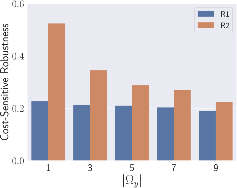
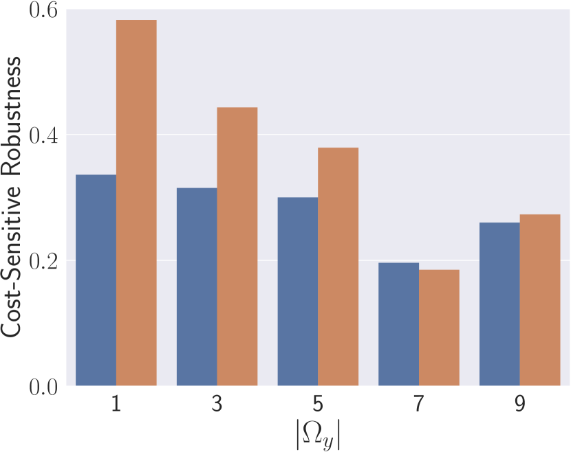
In summary, if $p_{B}$, the ground-truth probability of the top class in $\Omega_{y}$, is far below $p_{A}$, then $R_{2}$ will be much higher than $R_{1}$, thus producing a much tighter cost-sensitive robust certificate. To further study the relationship between $R_{1}$ and $R_{2}$, we conduct experiments to compare the cost-sensitive robustness computed based on $R_{1}$ and $R_{2}$ across different cost matrix scenarios, as shown in Figures 1(a) and 1(b). We fix a single seed class “cat” as sensitive and vary the size of its corresponding cost-sensitive target classes, randomly selecting $|\Omega_{y}|\in\{1,3,5,7,9\}$ of all the possible target classes. We then evaluate the performance of the models produced by two baseline training methods for randomized smoothing, Cohen (Cohen et al., 2019) and MACER (Zhai et al., 2020). Figures 1(a) and 1(b) show that cost-sensitive robustness measured by $R_{2}$ outperforms that of $R_{1}$ across most of the settings. As the size of $\Omega_{y}$ decreases, the performance gap between $R_{1}$ and $R_{2}$ is more pronounced, underscoring the superior efficacy of $R_{2}$ and confirming the superiority of our proposed certification algorithm.

4 Training for Cost-Sensitive Robustness

A popular training scheme for cost-sensitive learning is reweighting (Elkan, 2001), which assigns larger weights to cost-sensitive inputs during model training. Thus, a natural question is whether the reweighting scheme can be incorporated in randomized smoothing to train for cost-sensitive robustness. In this section, we first study the effectiveness for cost-sensitive robustness of combining the reweighting methods with Cohen (Section 4.1), then provide a new training method by leveraging the design insight of MACER (Zhai et al., 2020) to achieve better performance (Section 4.2).

4.1 Reweighting Method

We consider the base classifier training method introduced in Cohen et al. (2019), which proposes to inject Gaussian noise to all inputs during the training process of $f_{\theta}$. Given a binary cost matrix, $\mathcal{D}$ is the underlying data distribution, let $\mathcal{D}_{s}$ be the distribution of all sensitive examples which incur costs if misclassified and let $\mathcal{D}_{n}$ represent the distribution of the remaining normal examples. Intuitively, the training pipeline of randomized smoothing can be adapted to cost-sensitive settings using a simple reweighting scheme by increasing the weights assigned to the loss function of sensitive examples, denoted as Cohen-R. More concretely, the training objective of Cohen-R is defined as follows:

$$\min_{\theta\in\Theta}\>\bigg{[}\mathbb{E}_{(\bm{x},y)\sim\mathcal{D}_{n}}\>\mathcal{L}_{CE}\big{(}f_{\theta}(\bm{x}+\bm{\delta}),y\big{)}+\alpha\cdot\mathbb{E}_{(\bm{x},y)\sim\mathcal{D}_{s}}\>\mathcal{L}_{CE}\big{(}f_{\theta}(\bm{x}+\bm{\delta}),y\big{)}\bigg{]},$$

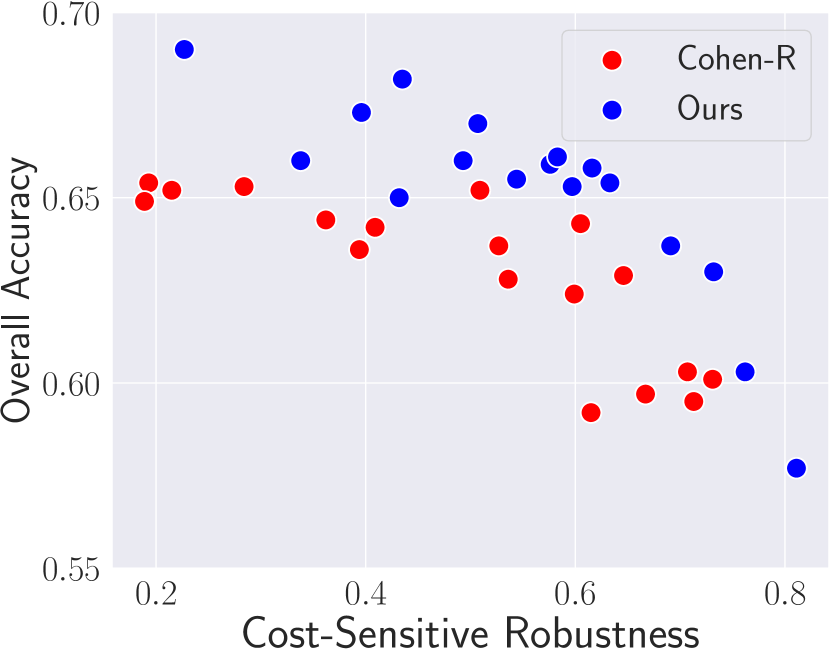
where $\Theta$ denotes the set of model parameters, $\mathcal{L}_{CE}$ represents the cross-entropy loss, and $\alpha\geq 1$ is a trade-off parameter that controls the performance between sensitive and non-sensitive examples. When $\alpha=1$, the above objective function is equivalent to the training loss used in standard randomized smoothing. However, due to the indirect optimization of the smoothed classifier, Cohen-R tends to sacrifice overall accuracy to a large degree when trying to achieve high cost-sensitive robustness (see Figure 1(c) for empirical evidence about this statement).

4.2 Our Method

In this section, we propose a more direct optimization scheme based on the proposed notion of certified cost-sensitive radius, leveraging a similar insight of MACER (Zhai et al., 2020) to better trade off cost-sensitive robustness and overall accuracy. To simplify notations, we first introduce a general class of margin-based losses. Given $l\leq u$ denoting the thresholding parameters, we define the following class of margin losses: for any $r\in\mathbb{R}$ representing the certified radius, let

$$\mathcal{L}_{M}\big{(}r;l,u\big{)}=\max\{u-r,0\}\cdot\mathbbm{1}(l\leq r\leq u).$$

Here, the indicator function selects data points whose certified radius falls into the range of $[l,u]$. For any binary cost matrix $\mathbf{C}$, the total training loss function of our method is defined as:

$$\min_{\theta\in\Theta}\>\> I_{1}+\lambda\cdot I_{2}+\lambda\cdot I_{3},$$ (2)

where $$I_{1}=\mathbb{E}_{(\bm{x},y)\sim\mathcal{D}}\>\mathcal{L}_{CE}\big{(}h_{\theta}(\bm{x}\big{)},y),$$

$$I_{2}=\mathbb{E}_{({\bm{x}},y)\sim\mathcal{D}}\>\mathcal{L}_{M}\big{(}R(\bm{x};h_{\theta});0,\gamma_{1}\big{)},$$

$$I_{3}=\mathbb{E}_{(\bm{x},y)\sim\mathcal{D}_{s}}\>\mathcal{L}_{M}\big{(}R_{\text{c-s}}(\bm{x};\Omega_{y},h_{\theta});-\gamma_{2},\gamma_{2}\big{)},$$

where $\lambda,\gamma_{1},\gamma_{2}>0$ are hyperparameters, and $\mathcal{D}$, $\mathcal{D}_{s}$ denote the underlying distributions of all and cost-sensitive examples, respectively. In particular, Equation 2 consists of three terms: $I_{1}$ represents the cross-entropy loss with respect to $h_{\theta}$ over $\mathcal{D}$, which controls the overall accuracy; $I_{2}$ denotes the margin loss based on the standard certified radius, similar to the design of MACER; $I_{3}$ optimizes the certified cost-sensitive robustness. The range of the interval $[l,r]$ used in the margin-based loss $\mathcal{L}_{\mathrm{M}}$ represents which data subpopulation we want to optimize. A larger thresholding parameter such as $\gamma_{1}$ and $\gamma_{2}$ lead to a higher data coverage, whereas the range with a smaller threshold includes fewer data points. We set $\gamma_{2}>\gamma_{1}$ to have a wider adjustment range for sensitive seed examples. As shown in Wang et al. (2020), optimizing misclassified samples can help adversarial robustness. Thus, we intend to include the set of sensitive seed examples with a negative radius in $[-\gamma_{2},0)$ in the design of $I_{3}$ for better performance. In addition, for pairwise cost matrices, we note that $[m]\backslash{\Omega_{y}}$ may contain target classes other than the ground-truth class $y$. As a result, optimizing $I_{3}$ inevitably encourages the standard accuracy trade-off from non-sensitive to cost-sensitive target classes, resulting in an undesirable degradation of overall accuracy. To alleviate this issue, we consider $\mathcal{D}$ instead of $\mathcal{D}_{n}$ in the objective of $I_{2}$ to particularly recalibrate the standard performance with the non-sensitive groups.

Intuitively speaking, by imposing different threshold restrictions $[l,u]$ on the certified radius of sensitive and non-sensitive seed classes, the optimization process can prioritize making adjustments to data subpopulations of specific classes rather than considering all data points belonging to those classes. This is also a key advantage of our method over the naive reweighting method. As will be shown in our experiments, such fine-grained optimization enables our method to improve certified cost-sensitive robustness to a large extent without sacrificing overall accuracy. Figure 1(c) provide empirical evidence of the non-optimal trade-off for the reweighting method Cohen-R on CIFAR-10 under a specific cost matrix of “cat” being the only sensitive seed class, compared with the performance of models produced by our proposed method. Each $(\mathrm{Rob}_{\text{c-s}},\mathrm{Acc})$ point is derived from a unique set of model tuning hyperparameters. Notably, the points corresponding to our method predominantly occupy the upper-right quadrant compared to those of Cohen-R, illustrating that our proposed approach offers a superior trade-off between cost-sensitive robustness and overall accuracy.

5 Experiments

Table 1: Certification results for seedwise cost matrices. The noise level $\sigma$ is $0.5$ and robustness is measured at $\epsilon=0.5$ in $\ell_{2}$-norm. Here, $\mathrm{Acc}$ stands for overall accuracy, and $\mathrm{Rob}_{\text{c-s}}$ is the cost-sensitive robustness computed using $\max(R_{1},R_{2})$ returned by Algorithm 1. As references, we also report $\mathrm{Rob}^{\text{(std)}}_{\text{c-s}}$, being the cost-sensitive robustness computed using standard radius $R_{1}$, and $\mathrm{Rob}^{\text{(std)}}_{\text{non}}$, being the robustness of non-sensitive samples using $R_{1}$. The best results are highlighted in bold.

Dataset	Type	Method	$\mathrm{Acc}$	$\mathrm{Rob}_{\text{c-s}}$	$\mathrm{Rob}^{\text{(std)}}_{\text{c-s}}$	$\mathrm{Rob}^{\text{(std)}}_{\text{non}}$
CIFAR-10	Single (3)	Cohen	$0.654$	$0.223$	$0.193$	$0.466$
		MACER	$0.659$	$0.273$	$0.259$	$0.499$
		Cohen-R	$0.642$	$0.506$	$0.466$	$0.437$
		Ours	$\bm{0.661}$	$\bm{0.628}$	$0.598$	$0.455$
	Multi (2, 4)	Cohen	$0.659$	$0.293$	$0.257$	$0.463$
		MACER	$0.659$	$0.291$	$0.262$	$0.527$
		Cohen-R	$0.662$	$0.348$	$0.308$	$0.413$
		Ours	$\bm{0.669}$	$\bm{0.461}$	$0.441$	$0.504$
Imagenette	Single ($7$)	Cohen	$\bm{0.803}$	$0.646$	$0.637$	$0.744$
		MACER	$0.782$	$0.638$	$0.638$	$0.739$
		Cohen-R	$0.746$	$0.733$	$0.733$	$0.671$
		Ours	$0.791$	$\bm{0.811}$	$0.795$	$0.725$
	Multi ($3,7$)	Cohen	$\bm{0.804}$	$0.589$	$0.579$	$0.771$
		MACER	$0.782$	$0.578$	$0.578$	$0.774$
		Cohen-R	$0.740$	$0.617$	$0.613$	$0.843$
		Ours	$0.791$	$\bm{0.715}$	$0.713$	$0.738$

In this section, we evaluate our method on two image benchmarks: CIFAR-10 (Krizhevsky et al., 2009) and Imagenette, a 10-class subset of ImageNet. Additionally, we test our method on the medical dataset HAM10k (Tschandl et al., 2018) to further examine its generalizability for real-world scenarios, where cost-sensitive misclassifications have more severe consequences. For CIFAR-10 and HAM10k, we use the same ResNet (He et al., 2016) architecture as employed in Cohen et al. (2019). Specifically, we choose ResNet-56, since it attains comparable performance to ResNet-110 but with less computation cost. For Imagenette, we use ResNet18 following Pethick et al. (2023).

We primarily compare our method with two prevalent randomized smoothing methods: Cohen (Cohen et al., 2019) and MACER (Zhai et al., 2020). We also consider Cohen-R, a variant of Cohen adapted for cost-sensitive scenarios using reweighting technique described in Section 4.1. We select Cohen for comparisons with standard randomized smoothing and MACER for comparing with methods that optimize for certified radius. Both of them are designed for overall robustness. Cohen-R is optimized for cost-sensitive performance by tuning the weight parameter $\alpha$ for a fair comparison. We mainly consider $\sigma=0.5$ and $\epsilon=0.5$, whereas results under other settings are provided in Appendix D.

Hyperparameter Tuning. The choice of hyperparameters plays a critical role in cost-sensitive learning. For Cohen-R, the weight parameter $\alpha$ is carefully tuned to ensure the best trade-off between overall accuracy and cost-sensitive robustness, where we enumerate all values from $\{1.0,1.1,\ldots,2.0\}$ and observe that nearly in all cases of cost matrices, setting $\alpha=1.2$ achieves the best result. For our method, we follow Zhai et al. (2020)’s setup for training. The main difference between our method and MACER is the choice of $\gamma$. MACER uses $\gamma=8$ to enhance the overall robustness for all classes, whereas we set $\gamma_{1}=4$ for normal classes and $\gamma_{2}=16$ for sensitive classes based on our analysis in Section 4.2. The effect of hyperparameters is further discussed in Appendix C.

5.1 Certification Results on Image Benchmarks

Seedwise Cost Matrix. Table 1 reports the overall accuracy and certified cost-sensitive robustness of our method and the three baselines with respect to different seedwise cost matrices. In particular, we consider two types of seedwise cost matrices in our experiments: Single: a randomly-selected sensitive seed class from all available classes, where we report the performance on the third class “cat” - label 3 for CIFAR-10 and “gas pump” - label 7 for Imagenette, and Multi: multiple sensitive seed classes, where “bird” - label 2 and “deer” - label 4 are considered as the sensitive seed classes for CIFAR-10, while we choose “chain saw” - label 3 and “gas pump” - label 7 for Imagenette. We observe similar trends for other settings of cost matrices, thereby omitting them here for simplicity.

We observe in Table 1 that our cost-sensitive robust training method achieves a significant improvement in terms of certified cost-sensitive robustness $\mathrm{Rob_{\text{c-s}}}$ compared with all of the three baselines. For all the seedwise cost matrix scenarios, our method achieves comparable or even slightly better performance than the baselines in terms of overall accuracy $\mathrm{Acc}$. In addition, we note that compared with MACER, there is a decrease in the certified robustness of non-sensitive examples with respect to our method, indicating a desirable shift of robustness from non-sensitive to sensitive examples, since we only optimize for certified robustness with respect to cost-sensitive examples. Moreover, we provide two methods for computing certified cost-sensitive robustness, where $\mathrm{Rob_{\text{{c-s}}}}$ is computed based on $\max\{R_{1},R_{2}\}$ returned by Algorithm 1, and $\mathrm{Rob}^{\text{(std)}}_{\text{c-s}}$ corresponds to the certified robustness of the sensitive seed examples but computed using $R_{1}$. Table 1 suggests that even for seedwise cost matrices with $|\Omega_{y}|=m-1$, our proposed certified cost-sensitive radius consistently outperforms the standard one, again confirming the superiority of Algorithm 1 in producing tighter bounds.

Table 2: Certification results for pairwise cost matrices. $\epsilon=0.5$ and $\sigma=0.5$ for both CIFAR-10 and Imagenette. $\mathrm{Acc}$ stands for overall accuracy, $\mathrm{Rob}_{\text{c-s}}$ refers to certified cost-sensitive robustness. The calculation of $\mathrm{Rob}_{\text{c-s}}^{\text{(std)}}$ and $\mathrm{Rob}_{\text{non}}^{\text{(std)}}$ is same as in Table 1. The best statistics are highlighted in bold.

Dataset	Type	Methods	$\mathrm{Acc}$	$\mathrm{Rob}_{\text{c-s}}$	$\mathrm{Rob}^{\text{(std)}}_{\text{c-s}}$	$\mathrm{Rob}_{\text{non}}^{\text{(std)}}$
CIFAR-10	Single ($3\rightarrow 5$)	Cohen	$0.654$	$0.504$	$0.227$	$0.443$
		MACER	$0.647$	$0.543$	$0.336$	$0.533$
		Cohen-R	$0.642$	$0.723$	$0.484$	$0.437$
		Ours	$\bm{0.673}$	$\bm{0.924}$	$0.441$	$0.472$
	Multi ($3\rightarrow 2,4,5$)	Cohen	$\bm{0.654}$	$0.336$	$0.213$	$0.446$
		MACER	$0.647$	$0.385$	$0.315$	$0.533$
		Cohen-R	$0.642$	$0.643$	$0.481$	$0.437$
		Ours	$0.643$	$\bm{0.822}$	$0.560$	$0.474$
Imagenette	Single ($7\rightarrow 2$)	Cohen	$\bm{0.803}$	$0.885$	$0.728$	$0.744$
		MACER	$0.782$	$0.899$	$0.792$	$0.749$
		Cohen-R	$0.754$	$0.911$	$0.811$	$0.679$
		Ours	$0.792$	$\bm{0.938}$	$0.804$	$0.731$
	Multi ($7\rightarrow 2,4,6$)	Cohen	$\bm{0.803}$	$0.756$	$0.684$	$0.744$
		MACER	$0.781$	$0.780$	$0.725$	$0.749$
		Cohen-R	$0.754$	$0.830$	$0.782$	$0.678$
		Ours	$0.796$	$\bm{0.863}$	$0.823$	$0.730$

Pairwise Cost Matrix. Similar to the seedwise case, we also consider two types of pairwise cost matrices: Single: a randomly-selected sensitive seed class with one sensitive target class, and Multi: a single sensitive seed class with multiple sensitive target classes. Table 2 compares the performance of our method with the three baselines for different pairwise cost matrices on CIFAR-10 and Imagenette. Similarly, our methods consistently yields the best certified cost-sensitive robustness $\mathrm{Rob}_{\text{c-s}}$ without affecting much of the performance of overall accuracy $\mathrm{Acc}$. Note that the superiority of our approach in preserving overall accuracy becomes even more pronounced when contrasted with the reweighting method Cohen-R, illustrating the better trade-off our proposed training algorithm is able to achieve. In addition, by comparing the performance with respect to $\mathrm{Rob}_{\text{c-s}}$ and $\mathrm{Rob}_{\text{non}}^{\text{(std)}}$ in Table 2, we can see that our method significantly improves cost-sensitive robustness by slightly sacrificing the robustness of non-sensitive examples, which will not incur any cost under the considered cost-sensitive settings. Table 2 also confirms our findings in Section 3.2 that $R_{2}$ is much tighter than $R_{1}$ for the purpose of certifying cost-sensitive robustness under pairwise cost matrix scenarios.

Table 3: Comparisons of different methods on the HAM10k dataset.

Method	$\mathrm{Acc}$	$\mathrm{Rob}_{\text{c-s}}$
Cohen	$0.829$	$0.118$
Cohen-R-I	$0.805$	$0.197$
Cohen-R-II	$0.784$	$\bm{0.437}$
MACER	$0.828$	$0.250$
Ours	$\bm{0.831}$	$0.413$

5.2 Real-World Performance

We report the results of our method on a real-world medical dataset: HAM10k, which is an imbalanced skin cancer dataset with 7 classes. The noise level here is set as $\sigma=0.5$ and the cost-sensitive robustness $\mathrm{Rob}_{\text{c-s}}$ is measured for $\epsilon=0.5$ in $\ell_{2}$-norm. Due to the small sample size or several classes in HAM10k, we group all images from the benign classes into a larger single category and all images from the malignant classes into another, which formulates a binary classification task. Since misclassifying a malignant tumor as benign typically has more severe consequences and results in higher costs for this medical application, we set any misclassiciation from malignant to benign as cost-sensitive, while regarding the cost of the other type of misclassifications as $0$. Table 3 demonstrates the overall accuracy and certified cost-sensitive robustness of the model produced by our cost-sensitive robust training method, compared with other alternatives. Cohen-R-I and Cohen-R-II represent two specific instantiations of Cohen-R with the weight parameter $\alpha$ selected as $1.1$ and $1.2$, respectively. As we increase the weight parameter $\alpha$, there is a noticeable enhancement in cost-sensitive robustness. However, this comes at the expense of a marked decline in overall accuracy, confirming the non-optimal trade-off phenomenon discussed in Section 4. Notably, our approach achieves a more desirable trade-off between the two metrics, underscoring its effectiveness for real-world applications.

5.3 Further Analysis

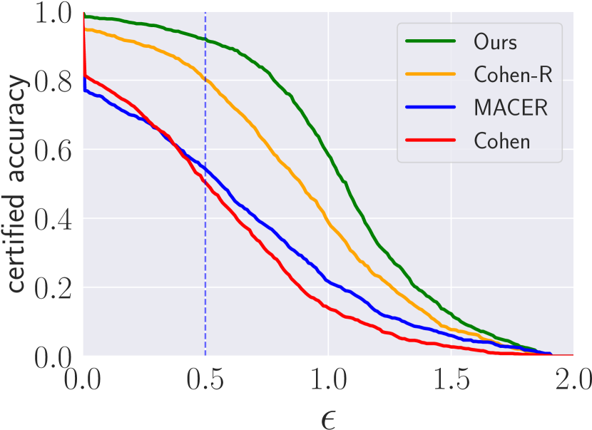
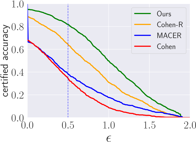
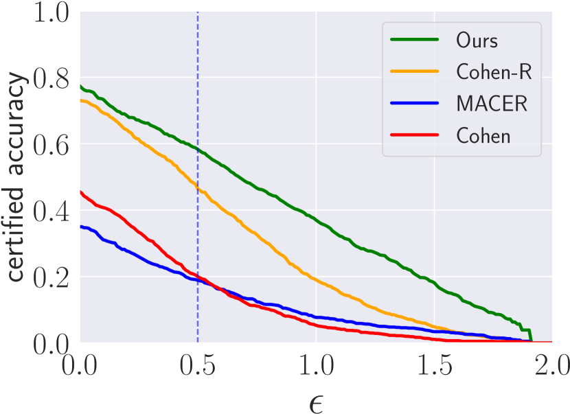
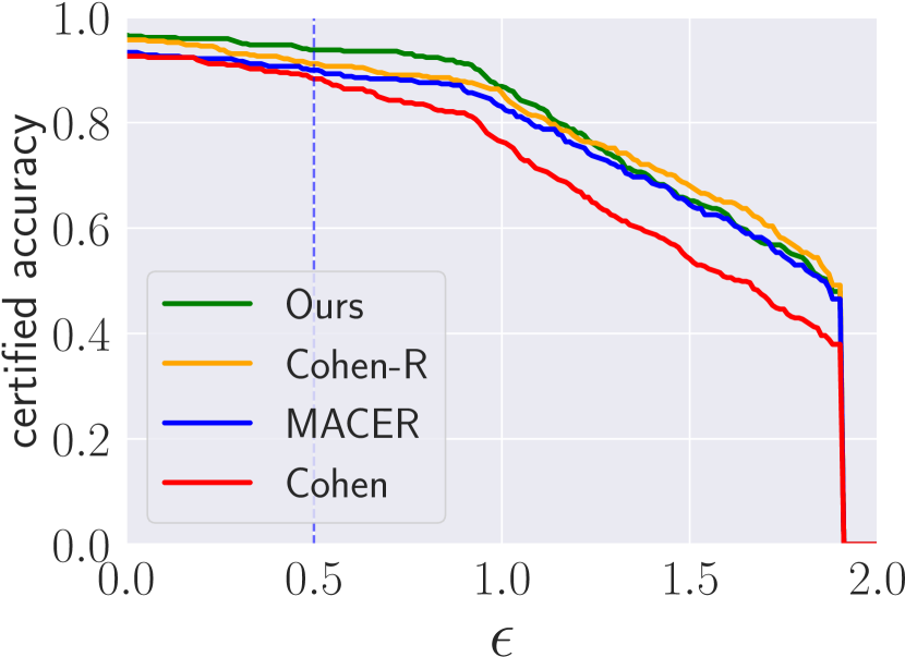
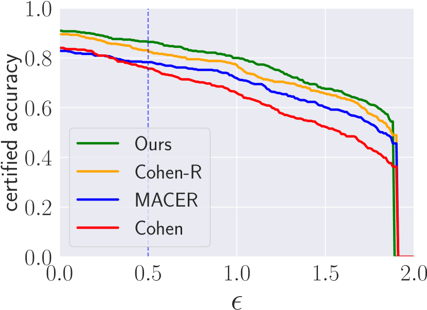
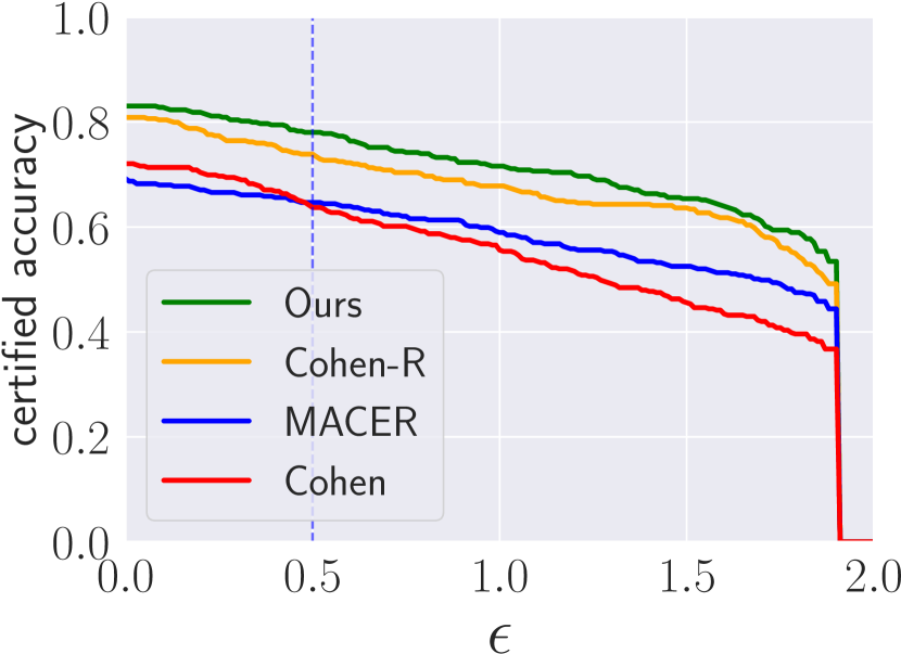
Certification Results with Varying $\epsilon$. To further visualize the consistency of our improvement, we compare the certified accuracy curves of cost-sensitive examples with varying $l_{2}$ perturbation for the aforementioned methods in Figure 2. The certified accuracy at $\epsilon=0$ measures certified accuracy for cost-sensitive examples drawn from the distribution $\mathcal{D}_{s}$, Meanwhile, the overall accuracy $\mathrm{Acc}$ listed in Tables 1 and 2 denotes the certified accuracy for all examples from the distribution $\mathcal{D}$. Both metrics compute the certified accuracy at $\epsilon=0$ but with respect to different data distributions. It is evident that our method consistently outperforms the baseline in terms of certified cost-sensitive accuracy across different $\epsilon$. In particular, we observe a significant improvement at $\epsilon=0.5$ of our method compared with other baselines. The certified accuracy $\epsilon=0.5$ aligns with $\mathrm{Rob}_{\text{c-s}}$ as presented in Tables 1 and 2, further corroborating our conclusions discussed in Section 5.1.

(a) Pairwise: ($3\rightarrow 5)$

(b) Pairwise: $(3\rightarrow 2,4,5)$

(c) Seedwise: $(3\rightarrow\text{all others})$

(d) Pairwise: ($7\rightarrow 2)$

(e) Pairwise: $(7\rightarrow 2,4,6)$

(f) Seedwise: $(7\rightarrow\text{all others})$

Figure 2: The curves of certified accuracy for varying $\epsilon$ under different cost-sensitive settings, where (a)-(c) in the top row correspond results for CIFAR-10, and (d)-(f) depict results for Imagenette.

Comparisons with Alternative Method. We also compare our method with Zhang & Evans (2019)’s, which provides a way to certify and train for cost-sensitive robustness based on the convex relaxation-based method (Wong & Kolter, 2018). However, the initial work of Wong & Kolter (2018) only focuses on $\ell_{\infty}$-norm bounded perturbations and does not consider perturbations in $\ell_{2}$-norm. Therefore, the proposed method in  Zhang & Evans (2019) is not applicable to certify cost-sensitive robustness for $\ell_{2}$ perturbations. We note that in a follow-up work of Wong et al. (2018), they extend the developed certification techinques to $\ell_{2}$ perturbations. For a fair comparison with our method, we adapt the cost-senstive robust learning method of Zhang & Evans (2019) to handle $\ell_{2}$-norm perturbations using the method of Wong et al. (2018). We report their comparisons in Table 4, the certified cost-sensitive robustness for the convex-relaxation method is computed as the cost-sensitive robust error defined in Zhang & Evans (2019). Table 4 shows that our method achieves much higher overall accuracy even against larger $\ell_{2}$ perturbations, suggesting a better cost-sensitive robustness and overall accuracy trade-off. Also, we find in our implementation that convex relaxation-based methods is not applicable to large $\ell_{2}$ perturbations (e.g., ${\epsilon}=0.5$), due to memory issues.

Table 4: Comparisons of our method with convex relaxation based method (Zhang & Evans, 2019) for $\ell_{2}$-norm on CIFAR-10, where a single pairwise transformation ($3\rightarrow 5$) is considered sensitive.

Method	$\ell_{2}$ Perturbations	Overall Accuracy	Cost-Sensitive Robustness
Zhang & Evans (2019)	$\epsilon=0.25$	$0.480$	$0.944$
Ours	$\epsilon=0.5$	$0.673$	$0.924$

6 Conclusion

We developed a generic randomized smoothing framework to certify and train for cost-sensitive robustness. At the core of our framework is a new notion of cost-sensitive certified radius, which is applicable to any binary cost matrix. Built upon fine-grained thresholding techniques for optimizing the certified radius with respect to different subpopulations, our method significantly improves the certified robustness performance for cost-sensitive transformations. Compared with naive reweighting approaches, our method achieves a much more desirable trade-off between overall accuracy and certified cost-sensitive robustness. Experiments on image benchmarks and real-world dataset demonstrate the superiority of our approach compared to various baselines. Our work opens up new possibilities for building certified robust models based on randomized smoothing for cost-sensitive applications.

Availability

Our implementation is available as open-source code at https://github.com/TrustMLRG/CS-RS.

Appendix

Appendix A Comparisons with Standard Certified Radius

The main distinction between our cost-sensitive certified radius $R_{\text{c-s}}(\bm{x};\Omega_{y})$ and Cohen et al. (2019)’s standard certified radius $R({\bm{x}})$ lies in the case when $|\Omega_{y}|<m-1$. In the following, we provide the detailed proof of Theorem 3.3.

Proof of Theorem 3.3.

Recall Cohen’s certified radius is:

$$R(\bm{x})=\frac{\sigma}{2}\Big{[}\Phi^{-1}\big{(}[h_{\theta}(\bm{x})]_{y}\big{)}-\Phi^{-1}\big{(}\max_{k\neq y}\>[h_{\theta}(\bm{x})]_{k}\big{)}\Big{]},$$ (3)

Note the prerequisite in the definition of $R(\bm{x})$ guarantees that ${\bm{x}}$ is correctly classified, which means $y$ is both the ground-truth class and top-1 class. our cost-sensitive certified radius is:

$$R_{\text{c-s}}(\bm{x};\Omega_{y})=\frac{\sigma}{2}\bigg{[}\Phi^{-1}\Big{(}\max_{k\in[m]}\>\big{[}h_{\theta}(\bm{x})\big{]}_{k}\Big{)}-\Phi^{-1}\Big{(}\max_{k\in\Omega_{y}}\>\big{[}h_{\theta}(\bm{x})\big{]}_{k}\Big{)}\bigg{]},$$

If $|\Omega_{y}|=m-1$, $R_{\text{c-s}}(\bm{x};\Omega_{y})$ and $R({\bm{x}})$ are equivalent as the set of target classes in both definitions are identical, while if $|\Omega_{y}|<m-1$, the second term in cost-sensitive certified radius will be no bigger than that of Cohen’s certified radius, leading to $R_{\text{c-s}}(\bm{x};\Omega_{y})\geq R({\bm{x}})$.

To be more specific, we have the following observations:

1. When $|\Omega_{y}|=m-1$, $R_{\text{c-s}}(\bm{x};\Omega_{y})\Leftrightarrow R(\bm{x})$. Since $\Omega_{y}=\{j|j\neq y,j\in[m]\}$ encompasses all incorrect classes, the two probability terms are fully matched for both radius.

2. When $|\Omega_{y}|<m-1$, $R_{\text{c-s}}(\bm{x};\Omega_{y})\geq R({\bm{x}})$. This is because the class index scope in the second term of $R_{\text{c-s}}(\bm{x};\Omega_{y})$ is narrower than that in $R(\bm{x})$. Since $\Omega_{y}\subseteq\{j\neq y,j\in[m]\}$, the highest probability with respect to $|\Omega_{y}|$ will be no bigger than the highest probability related to all incorrect classes in $R(\bm{x})$. Consequently, $R_{\text{c-s}}(\bm{x};\Omega_{y})\geq R(\bm{x})$.

Therefore, we complete the proof of Theorem 3.3. ∎

Appendix B Additional Details for Section 3.2

This section provides more details about Algorithm 1 and the proof of Theorem 3.4.

Details of Algorithm 1. We follow the same sampling procedure of Cohen et al. (Cohen et al., 2019). To be more specific, the sampling function $\textsc{SampleUnderNoise}(f,\bm{x},n,\sigma)$ is defined as:

1. Draw $n$ i.i.d. samples of Gaussian noises $\bm{\delta}_{1}\ldots\bm{\delta}_{n}\sim\mathcal{N}(0,\sigma^{2}\mathbf{I})$.

2. Obtain the predictions $f(\bm{x}+\bm{\delta}_{1}),\ldots,f(\bm{x}+\bm{\delta}_{n})$ with base classifier $f$ on noisy images.

3. Return the counts for each class, where the count for class c is $\sum_{i\in[n]}\mathds{1}[f(\bm{x}+\bm{\delta}_{i})=c]$.

Proof of Theorem 3.4. We provide the proof of Theorem 3.4 presented in Section 3.2, where we make use of the union bound to prove the validity the upper confidence bound $\overline{p_{B}}$ with respect to $\Omega_{y}$.

Proof of Theorem 3.4.

Our goal is to show that $R_{2}$ specified in Algorithm 1 is a cost-sensitive certified radius with at least $1-\alpha$ confidence over the randomness of the Gaussian sampling. Let $m$ be the number of total label classes, and let $(p_{1},\dots,p_{m})$ be the ground-truth probability distribution of the smoothed classifier $g_{\theta}$ for a given example $(\bm{x},y)$. Denote by $p_{A},p_{B}$ the maximum probabilities in $[m]$ and in $\Omega_{y}$, respectively. According to the design of Algorithm 1, we can compute the empirical estimate of $p_{k}$ for any $k\in[m]$ based on $n$ Gaussian samples and the base classifier $f_{\theta}$. Let $(\hat{p}_{1},\dots,\hat{p}_{m})$ be the corresponding empirical estimates, then we immediately know

$$\hat{p}_{k}\sim\mathrm{Binomial}(n,p_{k}),\text{for any }k\in[m].$$

For $R_{1}$, we follow the same procedure as in Cohen et al. (2019) to compute the $1-\alpha$ lower confidence bound on $p_{A}$, which is guaranteed by the fact that $p_{B}\leq 1-p_{A}$. However, for the computation of $R_{2}$, we need compute both a lower confidence bound on $p_{A}$ and a upper confidence bound on $p_{B}$, which requires additional care to make the computation rigorous. In particular, we adapt the definition of standard certified radius (Theorem 1 in Cohen et al. (2019)) to cost-sensitive scenarios for deriving $R_{2}$. According to the construction of $\underline{p_{A}}=\mathrm{LowerConfBnd}(\mathrm{count}[\hat{c}_{A}],n,1-\alpha/2]$, we have

$$\mathrm{Pr}\Big{[}\underline{p_{A}}\leq p_{A}\Big{]}\geq 1-\frac{\alpha}{2}.$$

Therefore, the remaining task is to prove

$$\mathrm{Pr}\Big{[}\overline{p_{B}}\geq p_{B}\Big{]}\geq 1-\frac{\alpha}{2},$$ (4)

where $\overline{p_{B}}$ is defined according to line 8 of Algorithm 1, and $\Omega_{y}$ denotes the set of cost-sensitive target classes. Note that $p_{B}=\max_{k\in\Omega_{y}}\{p_{k}\}$ is used to define $R_{\text{c-s}}(\bm{x},\Omega_{y})$. If the above inequality holds true, we immediately know that by union bound,

$$\mathrm{Pr}\Big{[}R_{2}\leq R_{\text{c-s}}(\bm{x};\Omega_{y})\Big{]} =\mathrm{Pr}\bigg{[}\frac{\sigma}{2}\big{(}\Phi^{-1}(\underline{p_{A}})-\Phi^{-1}(\overline{p_{B}})\big{)}\leq\frac{\sigma}{2}\big{(}\Phi^{-1}(p_{A})-\Phi^{-1}(p_{B})\big{)}\bigg{]}$$

$$\geq 1-\Big{(}\mathrm{Pr}\Big{[}\underline{p_{A}}\geq p_{A}\Big{]}+\mathrm{Pr}\Big{[}\overline{p_{B}}\leq p_{B}\Big{]}\Big{)}\geq 1-\alpha.$$

The challenge for proving Equation 4 lies in the that we do not know the top class within $\Omega_{y}$ which is different from the case of $\underline{p_{A}}$. Therefore, we resort to upper bound the maximum over all the ground-truth class probabilities within $\Omega_{y}$. Based on the distribution of $\hat{p}_{k}$, we know for any $k\in\Omega_{y}$,

$$\mathrm{Pr}\Big{[}\overline{p_{k}}\geq p_{k}\Big{]}\geq 1-\alpha/(2|\Omega_{y}|),$$

where $\overline{p_{k}}$ is defined as the $1-\alpha/(2|\Omega_{y}|)$ upper confidence bound computed using $\hat{p}_{k}$. We remark that the choice of $1-\alpha/(2|\Omega_{y}|)$ can in fact be varied for each $k\in\Omega_{y}$ and even optimized for obtaining tighter bounds, as long as the summation of the probabilities of bad event happening is at most $\alpha/2$. Here, we choose the same value of $1-\alpha/(2|\Omega_{y}|)$ across different $k$ only for simplicity. According to union bound, we have

$$\mathrm{Pr}\bigg{[}\max_{k\in\Omega_{y}}\overline{p_{k}}\geq p_{B}\bigg{]}=\mathrm{Pr}\bigg{[}\max_{k\in\Omega_{y}}\overline{p_{k}}\geq\max_{k\in\Omega_{y}}p_{k}\bigg{]} \geq 1-\sum_{k\in\Omega_{y}}\mathrm{Pr}\Big{[}\overline{p_{k}}\leq p_{k}\Big{]}$$

$$\geq 1-|\Omega_{y}|\cdot\alpha/(2|\Omega_{y}|)=1-\frac{\alpha}{2},$$

where the first inequality holds because of union bound, which completes the proof. ∎

Appendix C Hyperparameter Tuning

In this section, we study the effect of hyperparameters $\gamma_{1}$ and $\gamma_{2}$ used in our method proposed in Section 4.2 on the two evaluation metrics, certified overall accuracy: and cost-sensitive robustness. Note that our goal is to improve cost-sensitive robustness without sacrificing overall accuracy, where $\gamma_{1}$ controls the margin of normal classes and $\gamma_{2}$ controls the margin of sensitive classes. In particular, we report the parameter tuning results on CIFAR-10. Here, the cost matrix is selected as a seedwise cost matrix with a sensitive seed class “cat”. We choose the specific “cat” class only for the purpose of illustration, as we observe similar trends in our experiments for other cost matrices, similar to the results shown in Table 1. In addition, we consider two comparison baselines:

• MACER (Zhai et al., 2020) with $\gamma=8$, restricting only on correctly classified examples.

• Our method with $\gamma_{1}=8$ and $\gamma_{2}=8$, the only difference with MACER is that our method contains misclassified examples for sensitive classes.

Below, we show the effect of $\gamma_{1}$ and $\gamma_{2}$ on the performance of our method, respectively.

(a) Overall

(b) Cost-Sensitive

Figure 3: Visualizations of our method with $\gamma_{1}\in\{4,6,8\}$ and fixed $\gamma_{2}=10$ with comparisons to baseline methods with: (a) overall performance and (b) cost-sensitive performance. Here, we consider a single cost-sensitive seed class “Cat” for the cost matrix.

(a) Overall ($\gamma_{1}=4$)

(b) Cost-Sensitive ($\gamma_{1}=4$)

(c) Overall ($\gamma_{1}=8$)

(d) Cost-Sensitive ($\gamma_{1}=8$)

Figure 4: Visualizations of our method for two groups comparisons to baseline methods in terms of (a)(c) overall performance and (b)(d) cost-sensitive performance. The first with $\gamma_{2}\in\{8,12,16\}$ and fixed $\gamma_{1}=4$, the second with $\gamma_{2}\in\{8,12,16\}$ and fixed $\gamma_{1}=8$. The cost matrix is set as the matrix representing a single cost-sensitive seed class “Cat”.

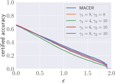
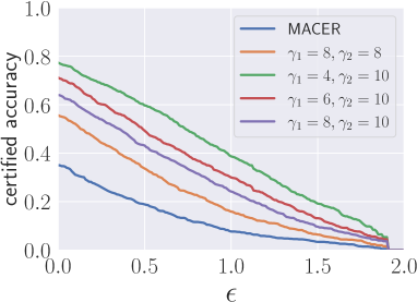
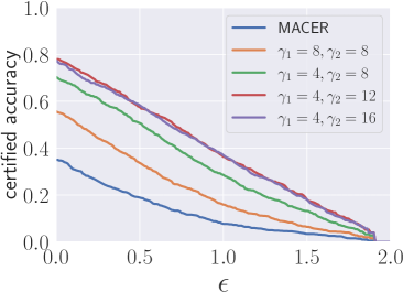
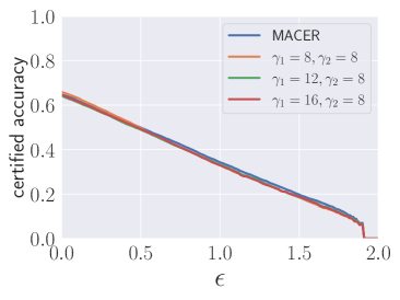
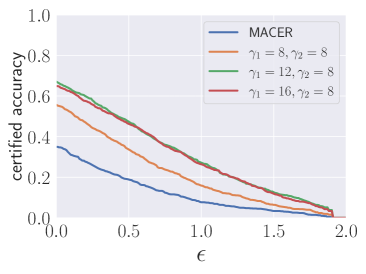
Effect of $\gamma_{1}$. Note that $\gamma_{1}$ is used to restrict the certified radius with respect to normal data points. Figure 3 illustrates the influence of varying $\gamma_{1}\in\{4,6,8\}$ and fixed $\gamma_{2}=10$ for our method, with comparisons to the two baselines, on both overall accuracy presented in Figure 3(a) and cost-sensitive robustness presented in Figure 3(b).

For the original implementation of MACER, $\gamma$ is selected as $8$ for the best overall performance. Although it achieves good overall robustness, it does not work for cost-sensitive settings, which suggests the possibility of a trade-off space, where different classes can be balanced to achieve our desired goal of cost-sensitive robustness. The second baseline is our method with $\gamma_{1}=8$ and $\gamma_{2}=8$. By incorporating misclassified samples for sensitive seed class, the cost-sensitive performance substantially improves. These results show the significance of including misclassified sensitive samples during the optimization process of the certified radius. Moreover, we can observe from Figure 3(b) that as we reduce the value of $\gamma_{1}$, the robustness performance of the cost-sensitive seed class increases. This again confirms that by limiting the certified radius of normal classes to a small threshold in our method, the model can prioritize sensitive classes and enhance cost-sensitive robustness. As depicted in Figure 3(a), the overall certified accuracy shows negligible variation, underscoring the efficacy of our training method in preserving overall accuracy.

Table 5: Performance of our method for different combinations of $\gamma_{1}$ and $\gamma_{2}$. Here, the cost-sensitive scenario is captured by the seedwise cost matrix with a single sensitive seed class “Cat” for CIFAR-10.

Method	$\gamma_{1}$	$\gamma_{2}$	$\mathrm{Acc}$	$\mathrm{Rob}_{\text{c-s}}$
MACER	-	-	$0.647$	$0.189$
Ours	8	8	$0.660$	$0.338$
Ours	2	8	$0.654$	$0.633$
	2	10	$0.634$	$0.687$
	2	12	$0.637$	$0.691$
	2	16	$0.630$	$0.705$
Ours	4	8	$0.670$	$0.507$
	4	10	$0.653$	$0.597$
	4	12	$0.659$	$0.576$
	4	16	$0.661$	$0.583$
Ours	6	8	$0.673$	$0.396$
	6	10	$0.660$	$0.493$
	6	12	$0.655$	$0.544$
	6	16	$0.649$	$0.552$
Ours	8	8	$0.660$	$0.338$
	8	10	$0.650$	$0.432$
	8	12	$0.641$	$0.474$
	8	16	$0.645$	$0.463$

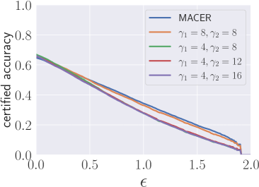
Effect of $\gamma_{2}$. Figure 4 illustrates the influence of varying $\gamma_{2}\in\{8,12,16\}$ with fixed $\gamma_{1}=4$ or fixed $\gamma_{1}=8$ for our method, with comparisons to the two baselines, on both overall accuracy and cost-sensitive robustness. Moreover, we can observe from Figure 4(b) and Figure 4(d) that as we increase the value of $\gamma_{2}$, the robustness performance of the cost-sensitive seed class increases. This confirms that by optimizing the certified radius of sensitive classes to a large threshold in our method, the model can focus more on sensitive classes and enhance cost-sensitive robustness. Additionally, there is a slight increase in the overall certified accuracy. This can be attributed to the fact that the overall accuracy takes into account both the accuracy of sensitive samples and normal samples. As the certified accuracy of sensitive samples increases, it dominates the overall accuracy and leads to its overall improvement. Table 5 demonstrates the impact of different combinations of hyperparameters of $(\gamma_{1},\gamma_{2})$ on both the overall accuracy and cost-sensitive performance. The choice of $\gamma_{1}$ and $\gamma_{2}$ is crucial and requires careful consideration. For $\gamma_{2}$, setting a value that is too small can greatly undermine the overall accuracy, even though it may improve cost-sensitive robustness. This is because the performance of normal classes deteriorates, resulting in a degradation of overall performance. Otherwise, if the value is too large (i.e., $\gamma_{2}=8$), it has a negative impact on cost-sensitive performance.

Regarding $\gamma_{1}$, it is evident that increasing its value while keeping $\gamma_{2}$ fixed leads to a significant improvement in cost-sensitive robustness. It is worth noting that even though the cost-sensitive seed class represents only a single seed, accounting for only $10\%$ of the total classes, enhancing its robustness has a positive effect on overall accuracy as well. For instance, let’s compare the combination $(\gamma_{1}=8,\gamma_{2}=4)$ to $(\gamma_{1}=8,\gamma_{2}=8)$. We observe that the former, which exhibits better cost-sensitive robustness, outperforms the latter in terms of both overall accuracy and cost-sensitive robustness. It achieves an approximate improvement of $1.52\%$ in overall accuracy and a significant improvement of approximately $50\%$ in cost-sensitive robustness. This finding highlights the effectiveness of our subpopulation-based methods. It demonstrates that by fine-tuning the optimization thresholds for the certified radius of sensitive classes and normal classes separately, we can achieve a better trade-off between overall accuracy and cost-sensitive robustness. The certified overall accuracy is depicted in Figure 4(a) and Figure 4(c), similar to the above analysis, these trends suggest our method’s effectiveness in maintaining overall accuracy.

Appendix D Varying Noise

Moreover, We test the performance of our method when the standard deviation parameter of the injected Gaussian noises is $\sigma=0.25$. We demonstrate the results in Table 6 and Table 7 respectively for seedwise and pairwise cost matrices. The results show that our method consistently outperforms the two baseline randomized smoothing methods and the reweighting method of Cohen-R.

Table 6: Certification results of different training methods for various seedwise cost matrices. The noise level $\sigma$ is $0.25$ for both CIFAR-10 and Imagenette. $\mathrm{Acc}$ stands for overall accuracy, $\mathrm{Rob}_{\text{c-s}}$ is certified cost-sensitive robustness with $\epsilon=0.25$. Best statistics are highlighted in bold.

Dataset	Type	Method	$\mathrm{Acc}$	$\mathrm{Rob}_{\text{c-s}}$
CIFAR-10	Single (3)	Cohen	$0.793$	$0.407$
		MACER	$0.808$	$0.475$
		Cohen-R	$0.778$	$0.583$
		Ours	$\bm{0.804}$	$\bm{0.602}$
	Multi (2, 4)	Cohen	$0.793$	$0.588$
		MACER	$\bm{0.808}$	$0.653$
		Cohen-R	$0.784$	$0.635$
		Ours	$0.807$	$\bm{0.717}$
Imagenette	Single ($7$)	Cohen	$0.803$	$0.656$
		MACER	$0.796$	$0.701$
		Cohen-R	$0.738$	$0.742$
		Ours	$\bm{0.836}$	$\bm{0.756}$
	Multi ($3,7$)	Cohen	$0.803$	$0.612$
		MACER	$0.796$	$0.662$
		Cohen-R	$0.764$	$0.656$
		Ours	$\bm{0.830}$	$\bm{0.702}$

Table 7: Certification results for pairwise cost matrices. The noise level $\sigma$ is $0.25$ for both CIFAR-10 and Imagenette. $\mathrm{Acc}$ stands for overall accuracy and $\mathrm{Rob}_{\text{c-s}}$ refers to certified cost-sensitive robustness measured at $\epsilon=0.25$.The best results are highlighted in bold.

Dataset	Type	Method	$\mathrm{Acc}$	$\mathrm{Rob}_{\text{c-s}}$
CIFAR-10	Single ($3\rightarrow 5$)	Cohen	$0.793$	$0.674$
		MACER	$0.808$	$0.709$
		Cohen-R	$0.778$	$0.811$
		Ours	$\bm{0.809}$	$\bm{0.836}$
	Multi ($3\rightarrow 2,4,5$)	Cohen	$0.793$	$0.515$
		MACER	$0.808$	$0.582$
		Cohen-R	$0.778$	$0.685$
		Ours	$\bm{0.807}$	$\bm{0.689}$
Imagenette	Single ($7\rightarrow 2$)	Cohen	$0.803$	$0.880$
		MACER	$0.796$	$0.837$
		Cohen-R	$0.764$	$0.921$
		Ours	$\bm{0.830}$	$\bm{0.942}$
	Multi ($7\rightarrow 2,4,6$)	Cohen	$0.803$	$0.730$
		MACER	$0.796$	$0.780$
		Cohen-R	$0.764$	$0.831$
		Ours	$\bm{0.832}$	$\bm{0.842}$

References

- Asif et al. (2015) Kaiser Asif, Wei Xing, Sima Behpour, and Brian D Ziebart. Adversarial cost-sensitive classification. In UAI, pp. 92–101, 2015.
- Athalye et al. (2018) Anish Athalye, Nicholas Carlini, and David Wagner. Obfuscated gradients give a false sense of security: Circumventing defenses to adversarial examples. In International conference on machine learning, pp. 274–283. PMLR, 2018.
- Carlini & Wagner (2017) Nicholas Carlini and David Wagner. Towards evaluating the robustness of neural networks. In 2017 ieee symposium on security and privacy (sp), pp. 39–57. Ieee, 2017.
- Carlini et al. (2022) Nicholas Carlini, Florian Tramer, Krishnamurthy Dj Dvijotham, Leslie Rice, Mingjie Sun, and J Zico Kolter. (certified!!) adversarial robustness for free! In The Eleventh International Conference on Learning Representations, 2022.
- Chen et al. (2021) Yizheng Chen, Shiqi Wang, Weifan Jiang, Asaf Cidon, and Suman Jana. Cost-aware robust tree ensembles for security applications. In USENIX Security Symposium, pp. 2291–2308, 2021.
- Cohen et al. (2019) Jeremy Cohen, Elan Rosenfeld, and Zico Kolter. Certified adversarial robustness via randomized smoothing. In international conference on machine learning, pp. 1310–1320. PMLR, 2019.
- Domingos (1999) Pedro Domingos. Metacost: A general method for making classifiers cost-sensitive. In Proceedings of the fifth ACM SIGKDD international conference on Knowledge discovery and data mining, pp. 155–164, 1999.
- Elkan (2001) Charles Elkan. The foundations of cost-sensitive learning. In International joint conference on artificial intelligence, volume 17, pp. 973–978. Lawrence Erlbaum Associates Ltd, 2001.
- Gan et al. (2021) Jiangzhang Gan, Jiaye Li, and Yangcai Xie. Robust svm for cost-sensitive learning. Neural Processing Letters, pp. 1–22, 2021.
- Goodfellow et al. (2014) Ian J Goodfellow, Jonathon Shlens, and Christian Szegedy. Explaining and harnessing adversarial examples. arXiv preprint arXiv:1412.6572, 2014.
- Gowal et al. (2018) Sven Gowal, Krishnamurthy Dvijotham, Robert Stanforth, Rudy Bunel, Chongli Qin, Jonathan Uesato, Relja Arandjelovic, Timothy Mann, and Pushmeet Kohli. On the effectiveness of interval bound propagation for training verifiably robust models. arXiv preprint arXiv:1810.12715, 2018.
- Hartnett et al. (2019) Gavin S Hartnett, Andrew J Lohn, and Alexander P Sedlack. Adversarial examples for cost-sensitive classifiers. arXiv preprint arXiv:1910.02095, 2019.
- He et al. (2016) Kaiming He, Xiangyu Zhang, Shaoqing Ren, and Jian Sun. Deep residual learning for image recognition. In Proceedings of the IEEE Conference on Computer Vision and Pattern Recognition (CVPR), June 2016.
- Jia et al. (2019) Jinyuan Jia, Xiaoyu Cao, Binghui Wang, and Neil Zhenqiang Gong. Certified robustness for top-k predictions against adversarial perturbations via randomized smoothing. arXiv preprint arXiv:1912.09899, 2019.
- Katsumata & Takeda (2015) Shuichi Katsumata and Akiko Takeda. Robust cost sensitive support vector machine. In Artificial intelligence and statistics, pp. 434–443. PMLR, 2015.
- Katz et al. (2017) Guy Katz, Clark Barrett, David L Dill, Kyle Julian, and Mykel J Kochenderfer. Reluplex: An efficient smt solver for verifying deep neural networks. In Computer Aided Verification: 29th International Conference, CAV 2017, Heidelberg, Germany, July 24-28, 2017, Proceedings, Part I 30, pp. 97–117. Springer, 2017.
- Khan et al. (2017) Salman H Khan, Munawar Hayat, Mohammed Bennamoun, Ferdous A Sohel, and Roberto Togneri. Cost-sensitive learning of deep feature representations from imbalanced data. IEEE transactions on neural networks and learning systems, 29(8):3573–3587, 2017.
- Krizhevsky et al. (2009) Alex Krizhevsky, Geoffrey Hinton, et al. Learning multiple layers of features from tiny images. 2009.
- Kurakin et al. (2016) Alexey Kurakin, Ian Goodfellow, and Samy Bengio. Adversarial machine learning at scale. arXiv preprint arXiv:1611.01236, 2016.
- Lecuyer et al. (2019) Mathias Lecuyer, Vaggelis Atlidakis, Roxana Geambasu, Daniel Hsu, and Suman Jana. Certified robustness to adversarial examples with differential privacy. In 2019 IEEE Symposium on Security and Privacy (SP), pp. 656–672. IEEE, 2019.
- Li et al. (2019) Bai Li, Changyou Chen, Wenlin Wang, and Lawrence Carin. Certified adversarial robustness with additive noise. Advances in neural information processing systems, 32, 2019.
- Liu et al. (2018) Xuanqing Liu, Minhao Cheng, Huan Zhang, and Cho-Jui Hsieh. Towards robust neural networks via random self-ensemble. In Proceedings of the European Conference on Computer Vision (ECCV), pp. 369–385, 2018.
- Madry et al. (2017) Aleksander Madry, Aleksandar Makelov, Ludwig Schmidt, Dimitris Tsipras, and Adrian Vladu. Towards deep learning models resistant to adversarial attacks. arXiv preprint arXiv:1706.06083, 2017.
- Mohapatra et al. (2020) Jeet Mohapatra, Ching-Yun Ko, Tsui-Wei Weng, Pin-Yu Chen, Sijia Liu, and Luca Daniel. Higher-order certification for randomized smoothing. Advances in Neural Information Processing Systems, 33:4501–4511, 2020.
- Papernot et al. (2016) Nicolas Papernot, Patrick McDaniel, Xi Wu, Somesh Jha, and Ananthram Swami. Distillation as a defense to adversarial perturbations against deep neural networks. In 2016 IEEE symposium on security and privacy (SP), pp. 582–597. IEEE, 2016.
- Pethick et al. (2023) Thomas Pethick, Grigorios Chrysos, and Volkan Cevher. Revisiting adversarial training for the worst-performing class. Transactions on Machine Learning Research, 2023. ISSN 2835-8856.
- Raghunathan et al. (2018) Aditi Raghunathan, Jacob Steinhardt, and Percy Liang. Certified defenses against adversarial examples. In International Conference on Learning Representations, 2018.
- Salman et al. (2019) Hadi Salman, Jerry Li, Ilya Razenshteyn, Pengchuan Zhang, Huan Zhang, Sebastien Bubeck, and Greg Yang. Provably robust deep learning via adversarially trained smoothed classifiers. Advances in Neural Information Processing Systems, 32, 2019.
- Salman et al. (2020) Hadi Salman, Mingjie Sun, Greg Yang, Ashish Kapoor, and J Zico Kolter. Denoised smoothing: A provable defense for pretrained classifiers. Advances in Neural Information Processing Systems, 33:21945–21957, 2020.
- Shafahi et al. (2019) Ali Shafahi, Mahyar Najibi, Mohammad Amin Ghiasi, Zheng Xu, John Dickerson, Christoph Studer, Larry S Davis, Gavin Taylor, and Tom Goldstein. Adversarial training for free! Advances in Neural Information Processing Systems, 32, 2019.
- Shen et al. (2022) Haojing Shen, Sihong Chen, Ran Wang, and Xizhao Wang. Adversarial learning with cost-sensitive classes. IEEE Transactions on Cybernetics, 2022.
- Tjeng et al. (2019) Vincent Tjeng, Kai Y. Xiao, and Russ Tedrake. Evaluating robustness of neural networks with mixed integer programming. In International Conference on Learning Representations, 2019.
- Tschandl et al. (2018) Philipp Tschandl, Cliff Rosendahl, and Harald Kittler. The ham10000 dataset, a large collection of multi-source dermatoscopic images of common pigmented skin lesions. Scientific data, 5(1):1–9, 2018.
- Wang et al. (2020) Yisen Wang, Difan Zou, Jinfeng Yi, James Bailey, Xingjun Ma, and Quanquan Gu. Improving adversarial robustness requires revisiting misclassified examples. In International Conference on Learning Representations, 2020.
- Wong & Kolter (2018) Eric Wong and Zico Kolter. Provable defenses against adversarial examples via the convex outer adversarial polytope. In International conference on machine learning, pp. 5286–5295. PMLR, 2018.
- Wong et al. (2018) Eric Wong, Frank Schmidt, Jan Hendrik Metzen, and J Zico Kolter. Scaling provable adversarial defenses. Advances in Neural Information Processing Systems, 31, 2018.
- Xiao et al. (2022) Chaowei Xiao, Zhongzhu Chen, Kun Jin, Jiongxiao Wang, Weili Nie, Mingyan Liu, Anima Anandkumar, Bo Li, and Dawn Song. Densepure: Understanding diffusion models for adversarial robustness. In The Eleventh International Conference on Learning Representations, 2022.
- Yang et al. (2020) Greg Yang, Tony Duan, J Edward Hu, Hadi Salman, Ilya Razenshteyn, and Jerry Li. Randomized smoothing of all shapes and sizes. In International Conference on Machine Learning, pp. 10693–10705. PMLR, 2020.
- Zhai et al. (2020) Runtian Zhai, Chen Dan, Di He, Huan Zhang, Boqing Gong, Pradeep Ravikumar, Cho-Jui Hsieh, and Liwei Wang. Macer: Attack-free and scalable robust training via maximizing certified radius. In International Conference on Learning Representations, 2020.
- Zhang et al. (2019) Hongyang Zhang, Yaodong Yu, Jiantao Jiao, Eric Xing, Laurent El Ghaoui, and Michael Jordan. Theoretically principled trade-off between robustness and accuracy. In International conference on machine learning, pp. 7472–7482. PMLR, 2019.
- Zhang et al. (2023) Jiawei Zhang, Zhongzhu Chen, Huan Zhang, Chaowei Xiao, and Bo Li. DiffSmooth: Certifiably robust learning via diffusion models and local smoothing. In 32nd USENIX Security Symposium (USENIX Security 23), pp. 4787–4804, 2023.
- Zhang & Evans (2019) Xiao Zhang and David Evans. Cost-sensitive robustness against adversarial examples. In International Conference on Learning Representations, 2019.