A Simple Way to Incorporate Novelty Detection in World Models

Abstract

Reinforcement learning (RL) using world models has found significant recent successes. However, when a sudden change to world mechanics or properties occurs then agent performance and reliability can dramatically decline. We refer to the sudden change in visual properties or state transitions as novelties. Implementing novelty detection within generated world model frameworks is a crucial task for protecting the agent when deployed. In this paper, we propose straightforward bounding approaches to incorporate novelty detection into world model RL agents, by utilizing the misalignment of the world model’s hallucinated states and the true observed states as an anomaly score. We first provide an ontology of novelty detection relevant to sequential decision making, then we provide effective approaches to detecting novelties in a distribution of transitions learned by an agent in a world model. Finally, we show the advantage of our work in a novel environment compared to traditional machine learning novelty detection methods as well as currently accepted RL focused novelty detection algorithms.

Introduction

Reinforcement learning (RL) using world models has found significant recent successes due to its strength in sampling efficiency and ability to incorporate well-studied Markov Decision Process techniques (Moerland et al. 2020)(Robine, Uelwer, and Harmeling 2021). A world model is a model that predicts the world state given a current state and the execution that was executed (or will be executed) (Ha and Schmidhuber 2018)

Figure 1: A world model-based reinforcement learning agent, DreamerV2 (Hafner et al. 2020), operating in nominal conditions (top) and after experiencing a novelty (bottom). Under nominal conditions the agent’s predicted state closely matches the ground-truth state. After experiencing novelty, the agent’s predicted state can radically diverge.

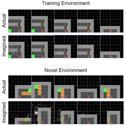
Many real-world scenarios such as autonomous driving (Kiran et al. 2020) and cybersecurity (Nguyen and Reddi 2021) face extreme risks when a fully-trained agent is exposed to novel or adversarial conditions during execution. Examples include a change to a visual stimulus that an agent previously relied on to make appropriate action choices, or a functional change to the transition dynamics of the environment such as a door no longer working the same way it used to. In cases where there is a novel change, the RL agent’s converged policy is no longer reliable and the agent can make catastrophic mistakes. In some cases, the agent may just flounder ineffectually. But in other cases, the agent can mistakenly take action that put itself in harms way or put others in harms way. While RL agents are often trained and evaluated in environments with stationary transition functions, the real world can undergo distributional shifts in the underlying transition dynamics.

Catastrophic failures are not purely a phenomenon in complex domains; it is trivial to set up an environment that introduces even simple novelties that completely undermine the agent’s learned policy (Balloch et al. 2022). Figure 1 shows that in many cases this can cause substantial disconnects between the ground truth of the world and the agent’s understanding of the world. In the figure (top), under nominal operation, the agent’s true state (top row) and the agent’s predicted state (second row) closely match. However, once a visual or functional novelty is introduced (third row), the agent’s predicted understanding of the world can be radically different to the point that the agent’s actions can no longer be trusted (fourth row). This shows that the agent’s errors are magnified when its world model and evaluation environment are not perfectly in sync (Moerland et al. 2020). As the agent’s model of the world and the true state of the world diverge, its chances of making erroneous behavior choices increase, putting the agent and others in the environment in danger. Thus, it is paramount that an agent operating in an environment where novelties can occur accurately recognize when a novelty has been introduced to cease operation or adapt (Balloch et al. 2022).

Though visual and functional novelty is a common occurrence in the real-world, the problem of detecting novel transitions in an online setting is not easily solved. One possibility is to use what the world model has learned during offline training to detect a novel transition as quickly as possible (i.e., with minimal detection lag) and with as few false positive or negatives as possible (Müller et al. 2022). In this paper we propose several straightforward bounding approaches such that the violation of the computed bounds indicate a high likelihood that the agent has encountered a novelty and is now in a world where its policy is no longer trustable. Our first approach involves computing the prior observation of the agent and measuring the formal Bayesian amount of “surprise” perceived by the agent in the form of reconstruction error. Our second approach uses the latent space model in DreamerV2’s world model (Hafner et al. 2020) to bound the measure of surprise based on assumptions of a trained model.

In this work, we consider the detection of two types of novelties: visual novelties and functional novelties. Visual novelties are considered to be observations where the image state representation has changed to an out-of-distribution visual with respect to the original training observations such as a new color and/or an addition/removal of an object. Functional novelties are instances where the learned Markov decision process produced from the training environment has solely had a change to its state-action transition distribution and/or action space without a visual cue.

The agent’s response to novelty is beyond the scope of this paper. We assume the agent is instructed to stop execution if novelty is detected, which suggests that any novelty detection must keep false positives to a minimum.

We evaluate these methods on variants of the minigrid environment (Chevalier-Boisvert, Willems, and Pal 2018) with the ability to inject a variety of novelties quickly (Balloch et al. 2022). Our results confirm that Bayesian surprise-based techniques successfully detect novel transitions. We compare our techniques against currently accepted RL focused novelty detection algorithms.

Related Work

Novelty detection has taken on different names depending on the context (Pimentel et al. 2014). There are important applications that can benefit from RL novelty detection frameworks (Fu, Co-Reyes, and Levine 2017), and yet novelty detection has not been well-studied to date in the realm of RL.

Many complications arise from applying traditional machine learning novelty detection methods to an online setting (Müller et al. 2022). Generalization techniques exist, such as procedural generation to train agents to be more robust to novel situations (Cobbe et al. 2019) and data augmentation (Lee et al. 2019) to better train the agent, however these techniques suffer from high sample complexity (Müller et al. 2022). Furthermore, there may not be a sufficient representation the agent’s evaluation environment to be able to detect novel Out-of-Distribution (OOD) transitions. Recent research shows that learning an OOD model is a difficult problem to solve and may even prove to be impossible in certain situations (Zhang, Goldstein, and Ranganath 2021) (Fang et al. 2022).

Some methods attempt to use a measure of reward signal deterioration as a way to detect if a novelty has occurred, but that can prove to be dangerous in a high stakes environment where it may be too late to recover from a negative signal.(Greenberg and Mannor 2020) This method may also prove to have am incorrect mapping to the novelty that caused the reward shift.

The framework RIQN (Danesh and Fern 2021) has proven to be successful by focusing on the aleoric uncertainty of the agent, and draws upon the generated distributions of Implicit Quartille networks (Dabney et al. 2018). Modeling after IQN, RIQN detects novelty by predicting action values from state-action pairs as input, and predicts the feature distribution at each time step, based on the previous values of the features.

There has been work on models that use bisimulation relations (Givan, Dean, and Greig 2003), which use equivalence relations to group states that are “behaviorally” similar in a Markov decision process (MDP) setting, i.e reward distributions and dynamics are similar. Since traditional bisimulation relations are strict in terms of generalization tasks, many models have relaxed the exactness requirement of the dynamics in favor of an $\epsilon$-bisimulation metrics approach (Gelada et al. 2019) to create a more generalized measure for state groupings (Ruan et al. 2015). More recently there has been work towards methods that use bisimulation metrics in world model RL frameworks, coined as latent space world models (Ha and Schmidhuber 2018), which focus on grouping similar dynamic states as the target for dimension reduction problems within Markov decision processes (Gelada et al. 2019).

Background

Partially observable Markov Decision Processes

We study episodic Partially Observable Markov decision processes (POMDPs) denoted by the tuple $M=(\mathcal{S},\mathcal{A},\mathcal{T},r,\Omega,O,\gamma)$, where $\mathcal{S}$ is the state space, $\mathcal{A}$ is the action space, $\mathcal{T}$ is the transition distribution $\mathcal{T}(s_{t}|s_{t-1},a_{t-1})$, r is the reward function, $O$ is the observation space, $\Omega$ is an emissions model from ground truth states to observations, and $\gamma$ is the discounting factor (Åström 1965).

DreamerV2 World Model

We conduct experiments applying our methods to the state-of-the-art DreamerV2 (Hafner et al. 2020) world model dynamics framework. DreamerV2 learns a policy by first learning a world model and then using the world model to roll out trials to train a policy model. The framework is composed of an image autoencoder and a Recurrent State-Space Model (RSSM). They represent each state $s_{t}$ in $\mathcal{S}$ as the compact model state $(h_{t},z_{t})$ where $h_{t}$ is the hidden deterministic component and $z_{t}$ is the stochastic component of the state that incorporates the learned dynamics of the current image observation $x_{t}$. Given each representation of state $s_{t}$, DreamerV2 defines six other learned, conditionally-independent transition distributions given by the trained world model:

$$\text{DreamerV2: }\begin{cases}\text{Recurrent model:}h_{t}=f_{\phi}(h_{t-1},z_{t-1},a_{t-1})\\ \text{Representation model: }p_{\phi}(z_{t}|h_{t},x_{t})\\ \text{Transition prediction model: }p_{\phi}(\hat{z_{t}}|h_{t})\\ \text{Image prediction model: }p_{\phi}(\hat{x_{t}}|h_{t},z_{t})\\ \text{Reward prediction model: }p_{\phi}(\hat{r_{t}}|h_{t},z_{t})\\ \text{Discount prediction model: }p_{\phi}(\hat{\gamma_{t}}|h_{t},z_{t})\end{cases}$$

where $\phi$ describes the parameter vector for all distributions optimized. The loss function during training (Hafner et al. 2020) is:

$$\begin{aligned} \mathcal{L}(\phi)=\mathop{\mathbb{E}}_{p_{\phi}(z|a,x)}\left[\sum_{t}^{T}\right.&-\text{ln}p_{\phi}(x_{t}|h_{t},z_{t})\\ &-\text{ln}p_{\phi}(r_{t}|h_{t},z_{t})\\ &-\text{ln}p_{\phi}(\gamma_{t}|h_{t},z_{t})\\ &+\beta KL\left[p_{\phi}(z_{t}|h_{t},x_{t})||p_{\phi}(z_{t}|h_{t})\right]\biggr{]}\end{aligned}$$ (1)

Where $\beta KL[p_{\phi}(z_{t}|h_{t},x_{t})||p_{\phi}(z_{t}|h_{t})$ is minimized by improving the prior dynamics towards the more informed posterior through KL Balancing (Hafner et al. 2020).

The goal of the DreamerV2 world model is to learn the dynamics, and predictors for the observation $x_{t}$, reward and discount factor of the training environment. We consider a single agent online RL setting, where an agent at time $t$ will traverse through each state $s_{t}$ in which observations are represented in the form of $x_{t}$. The agent will rely on these representations along with $r_{t}$ to construct its belief state and make decisions to achieve the optimal discounted sum of rewards.

We consider an agent that has trained in a stationary training environment and has been deployed to a non-stationary evaluation environment that undergoes a change that is a priori unknown and unanticipated by during agent development and training.

Bayesian Surprise

The Bayesian Theory of Surprise (Itti and Baldi 2005) suggests that the background information of an observer can be captured by a prior probability distribution over the model space. The intuition is that if the observation does not affect the prior distribution, then the observation carries no surprise, hence the level of surprise an observation brings can be measured by the KL divergence of the prior and posterior, given observation $x_{t}$:

$$\begin{aligned} KL[P(z_{t}|h_{t},x_{t})&||P(z_{t}|h_{t})]=\\ &\sum_{\mathbf{z}}P(z_{t}|h_{t},x_{t})\log\frac{P(z_{t}|h_{t},x_{t})}{P(z_{t}|h_{t})}\end{aligned}$$ (2)

Effective Novelty Detection

Our goal is to safely halt the agent in response to all possible Markovian novel observations. Therefore, we do not consider techniques that are reliant on reward deterioration as these methods can involve temporally extended action sequences to be conducted between sparse reward. Even with dense rewards, novelty may only be detected after some amount of time of decreased rewards. We also do not consider generalization techniques that are aimed to model possible novelties that the agent may experience, as it is currently impossible to construct a model that generalizes towards every unseen stimuli; indeed one must be able to categorize possible novelties in advance and generate novelties during training time (Wang et al. 2020)

Observation-based Detection Methods

We demonstrate two reconstruction observation-based detection methods directly dependent on the observation $x_{t}$: (1) Classical Multi-threshold Reconstruction Error and (2) post-prior mean absolute reconstruction error.

Classical Multi-threshold Reconstruction Error

For our first method, we leverage Classical Multi-Threshold Reconstruction Error (CMTRE), a commonly used approach for novel observation detection in traditional machine learning (Pimentel et al. 2014) under the assumption that the Mean Absolute Reconstruction Error (MARE) distribution of the novelties will be greater than the the mean of the distribution of MARE visuals $x_{t}$ from the original training environment, by some standard deviation between 1-0.5. Therefore to implement CTMRE in this setting, We construct a threshold of 0.5 standard deviation above the MARE from samples of the agent’s past experiences in its experience replay buffer, classifying observations with MARE above the threshold as novelty. Since the distribution of observations of a trained agent differ from the observations of an untrained agent, we experiment using three separate thresholds generated from three different means: (1) a trained agent’s MARE of observations; (2) an untrained agent’s MARE of observations; and (3) the equally distributed MARE of observations from both the trained and untrained agents.

Post-Prior MARE

In unsupervised learning, CMTRE is appealing since the reconstruction thresholds can be stored during training and makes for an efficient detection method during deployment. However, in the RL setting, problems can arise since this method assumes that the training environment is stationary and, therefore, relies on the “ground truth” of the replay buffer (Dao and Lee 2019). CMTRE also relies on the extent of the encoder’s convergence during the storing of the reconstruction errors, which can skew thresholds if collected too early in training.

We believe reconstruction error can indeed be a reliable detection method if used correctly in the Model-RL context. To illustrate, we instead derive a reconstruction error technique over the induced DreamerV2’s RSSM prior and posterior reconstructions. To evaluate the success, we consider the common technique of CMTRE to be a baseline, denoting (1) as the ”trained model” threshold, (2) as the ”random model” threshold, and (3) as the mean of thresholds i.e ”combination threshold”. Note that locally successful training of the world model implies that $\beta KL[p_{\phi}(z_{t}|x_{t},h_{t})||p_{\phi}(\hat{z_{t}}|h_{t}))]\leq\epsilon$. To properly utilize reconstruction error for trained world models, we induce $P(x_{t}|h_{t},\hat{z_{t}})$ from 1 where $h_{t}=f_{\phi}(h_{t-1},z_{t-1},a_{t-1})$, $z_{t-1}\sim P(z_{t-1}|h_{t-1},x_{t-1})$, and $\hat{z_{t}}\sim P(z_{t}|h_{t})$ to compare the $i$ pixel reconstruction losses between the generated 1-step prior and posterior $x_{t}$ observations and bound the difference by a small $\epsilon$ defined by the user during deployment:

$$\frac{\sum_{i}^{N}|\hat{x_{t}}^{i}_{prior}-\hat{x_{t}}^{i}_{posterior}|}{N}\leq\epsilon$$ (3)

where $\hat{x_{t}}_{\mathrm{prior}}\sim p_{\phi}(\hat{x_{t}}|h_{t},\hat{z_{t}})$, and $\hat{x_{t}}_{\mathrm{posterior}}\sim p_{\phi}(\hat{x_{t}}|h_{t},z_{t})$. This removes direct dependence on the replay buffer by using only the final performance of the encoder and the current state $(z_{t},h_{t})$. As seen in Figure 2, the prior and posterior can have dramatic changes in representation when the predicted latent representation $z_{t}$ is revealed.

Figure 2: From left to right, $\hat{x_{t}}_{prior},\hat{x_{t}}_{posterior}$ and $x_{t}$ observations of agent trying to open door in the broken door custom minigrid environment where the door fails to open despite having the correct key.

In addition to detecting novelties, this method also enables an agent to explain its expectations and beliefs to a human user based on the correlation between the latent state and the sampled image.

Latent-based Detection Methods

For latent-based detection, we investigate the world model and its learned probabilities. We construct a bound that is not dependent on hyper-parameters, and test the world model’s learned logic given the effect of $x_{t}$.

Dynamic KL Divergence Bounding (KL)

We establish a bound that tests the latent space model’s current performance. Unlike the observation-based detection methods, we can take advantage of an agent’s world model’s discrete latent space, as in DreamerV2, and use the compact one-hot encoding of $(s_{t-1},a_{t-1},r_{t},s_{t})$ transitions for our functional detection methods rather than making inferences on the observation, $x_{t}$, directly.

The KL loss function (Equation 1) implies that as training progresses the divergence between the latent representation of the hidden state given the latent current state representation with and without the direct observation goes to zero for local transitions, i.e., $KL[p_{\phi}(z_{t}|h_{t},x_{t})||p_{\phi}(z_{t}|h_{t})]\leq\epsilon$. Given the current training mechanism in place, learning the transition distribution may be difficult due to the task of avoiding regularizing the representations toward a poorly trained prior.

A direct consequence of using common KL balancing techniques such as 1 to bias the loss towards the prior error is that the world model is initially reliant on ground truth $x_{t}$ in contrast to a noisy $h_{t}$ to stabilize $p(z_{t}|h_{t},x_{t})$ for proper training of $p(z_{t}|h_{t})$ and $p(\hat{x_{t}}|h_{t},z_{t})$ (Asperti and Trentin 2020). Since the world model does not directly measure this relationship with $x_{t}$, we introduce the cross entropy score comparison:

$$H(p_{\phi}(z_{t}|h_{t},x_{t}),p_{\phi}(z_{t}|h_{0}))-$$ (4)

$$H(p_{\phi}(z_{t}|h_{t},x_{t}),p_{\phi}(z_{t}|h_{0},x_{t}))$$

where $h_{0}$ is simply a zero vector passed to the model in order to simulate the dropout of $h_{t}$ and compute the influence that the ground truth $x_{t}$ has on the final prediction of the distribution of $z_{t}$. This gives us an empirical measure of the world model’s current reliance and improved performance given the ground truth observation $x_{t}$, given that the cross entropy score comparison increases if we find the entropy to be minimized with respect to $h_{0}$.

As the divergence between latent predictions with and without the ground truth observable decreases, $KL[p_{\phi}(z_{t}|h_{t},x_{t})||p_{\phi}(z_{t}|h_{t})]\rightarrow\epsilon$, we expect a direct result of this to be the reduction of the impact of $x_{t}$. We model this relationship with the novelty detection bound:

$$KL[p_{\phi}(z_{t}|h_{t},x_{t}) ||p_{\phi}(z_{t}|h_{t})]\leq$$ (5)

$$KL[p_{\phi}(z_{t}|h_{t},x_{t})||p_{\phi}(z_{t}|h_{0})]$$

$$-KL[p_{\phi}(z_{t}|h_{t},x_{t})||p_{\phi}(z_{t}|h_{0},x_{t})]$$

where we substitute KL divergence in place of cross entropy loss to use the world model loss function 1.

The intuition behind the bound is as follows. For an unforeseen $\hat{x_{t}}$, if this relationship becomes disturbed—that is, if the model is incapable of constructing a mapping such that the the cross entropy of $H(p_{\phi}(z_{t}|h_{t},x_{t}),p_{\phi}(z_{t}|h_{0},x_{t}))$ is not minimized with respect to the performance of $H(p_{\phi}(z_{t}|h_{t},x_{t}),p_{\phi}(z_{t}|h_{0}))$—the threshold (the right-hand side of the equality in Equation 5 will decrease. But it is also expected that the left-hand side, $KL[p_{\phi}(z_{t}|h_{t},x_{t})||p_{\phi}(z_{t}|h_{t})]$, reaches extremely high values, depending on the current reliance of $h_{t}$.

Two cases of detection arise: If the world model performance somehow increases without data, then the right side will become negative, which is then immediately flagged as novelty due to the convexity of the KL divergence. If the the world model performance improves with data, then the bound becomes a dropout generalization test of the model (Srivastava et al. 2014) i.e:

$$KL[p_{\phi}(z_{t}|h_{t},x_{t}) ||p_{\phi}(z_{t}|h_{t})]+$$ (6)

$$KL[p_{\phi}(z_{t}|h_{t},x_{t})||p_{\phi}(z_{t}|h_{0},x_{t})]$$

$$\leq KL[p_{\phi}(z_{t}|h_{t},x_{t})||p_{\phi}(z_{t}|h_{0})]$$

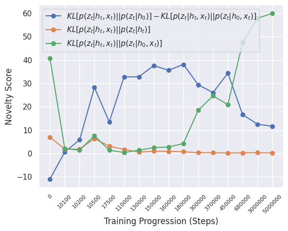
Where the model is tasked to simultaneously have sufficiently good performance with the dropout of $x_{t}$ and with the dropout of $h_{t}$. Therefore, our bound is both combating posterior collapse i.e $P_{\theta}(z|x)=P_{\theta}(z|0)$, as well as measuring possible over-fitting i.e $KL[P_{\theta}(z_{t}|h_{t},x_{t})||P_{\theta}(z_{t}|h_{0},x_{t})]>>c$ for some large c. Indeed, we find this empirically to be true, as shown in Figure 3. As the agent trains in a stationary (no novelty) environment, the surprise (orange) settles and steadily decreases. Initially, the difference of KL divergences (blue) flags all new stimuli novel, but DreamerV2 quickly learns that the environment is predictable. We see here that as the agent progresses through training, the green line symbolises how effective inputs ($h_{0}$, $x_{t}$), are to the model in terms of predicting a distribution which minimizes $KL[p_{\phi}(z_{t}|h_{t},x_{t})||p_{\phi}(z_{t}|h_{0},x_{t})]$. During training this value grows exponentially since the prediction is now approximately conditionally independent of $x_{t}$.

Figure 3: Visualization of the average levels of proposed bound (Blue), Novelty score given $x_{t}$ (Orange), and the divergence of $KL[p_{\phi}(z_{t}|h_{t},x_{t})||p_{\phi}(z_{t}|h_{0},x_{t})]$ (Green) as training progresses in the Nominal environment.

Optional Mahalanobis Extension

Given an environment that is typically deterministic, an optional latent-based novelty detection method considers a low variance for the learned transition distribution of the world model RSSM. We optionally consider the bound:

$$KL[p_{\phi}(z_{t}|h_{t},x_{t})||p_{\phi}(z_{t}|h_{t})]+\lambda d(z_{t}|p_{\phi}(z_{t}|h_{t},x_{t}))\leq$$ (7)

$$(KL[p_{\phi}(z_{t}|h_{t},x_{t})||p_{\phi}(z_{t}|h_{0},x_{t})]$$

$$-KL[p_{\phi}(z_{t}|h_{t},x_{t})||p_{\phi}(z_{t}|h_{0})])$$

where $\lambda$ is an optional relaxing hyperparameter, and $d(\cdot)$ is the Mahalanobis Distance (Lee et al. 2018), the distance from a point to a distribution.

At each step, we calculate the Mahalanobis distance from the discrete latent representation $z_{t}$ to the transition conditional distribution $P(z_{t}|h_{t},x_{t})$ using the world model’s learned transition probability model. We classify novelties above the threshold as a novel transition. This is a natural extension of the DreamerV2 world model framework. The latent features are already encoded as independent variables, allowing us to reduce the computation of the Mahalanobis distance dramatically since the covariance psuedo-inverse matrix of the distribution reduces to a diagonal matrix:

$$d_{M}(z_{t}|p_{\phi}(z_{t}|h_{t},x_{t})) =\sqrt{(z_{t}-\mu)^{T}\Sigma^{-1}(z_{t}-\mu)}$$ (8)

$$=\sum_{i}^{N}\Sigma^{-1}_{ii}(z_{t}-\mu)^{2}_{i}.$$

Experiments

Experiments are conducted in the Minigrid (Chevalier-Boisvert, Willems, and Pal 2018) environment. We implement custom environments to showcase a larger variety of non-trivial novelties than is currently available in the default Minigrid library. Each functional novelty environment is visually identical to the nominal environment. We describe each custom environment in Table 3 in the Appendix. For our experiments we use BrokenDoor, ActionFlip, Teleport, and FakeGoal as functional novelty environments. We use LavaGap, Empty, Fetch, and DoorGone as visual novelty environments. MiniGrid-Doorkey-6x6 serves as our nominal case.

We first train an agent to learn a $\epsilon$-optimal policy in the nominal environment, then transfer the agent to one of the several mini-grid environments with visual or functional novelties during testing time. We then let the trained agent take steps in each novel environment, capturing 50,000 steps within various independent and identically distributed episodes; tracking each time step where novelty is detected to imitate possible agent halting situations. The agent’s trained policy is expected to be sub-optimal in the novel environments and is not re-trained at any point to adapt to the novel environments’ dynamics.

We compare our methods against the Recurrent Implicit Quantile Network anomaly detection model (RIQN) (Danesh and Fern 2021), a traditional and accepted RL focused novelty detection approach, and take note of some of the practical desiderata discussed in (Müller et al. 2022) to ground our evaluation techniques. We explicitly train the RIQN model using nominal transitions given by a trained policy as recommended (Danesh and Fern 2021). We test the trained RIQN algorithm with the recommended hyper-parameters, as well as use the recommended cusum algorithm to detect novelties (Page 1954).

We trivially use $\epsilon=1$ for our Post-Prior MARE bound method during all experiments.

Average Delay Error

To evaluate performance of all methods, we measure how long it takes to detect the novelty To penalize preemptive and delayed detections, we define novelty detection delay error as the difference between the earliest time step that novelty is first observable and the time step that the novelty is detected. We calculate the agent’s average delay error (ADE) by averaging the absolute delay error across all novel environment episodes. We use the original nominal training environment to test for false positives; we do not consider false negatives when in the training environment. Ideal performance minimizes the average delay error and false positives/negatives (Müller et al. 2022).

Figure 4 shows average delay error for all novelty environments. For visual novelty environments, ActionFlip was the most difficult environment, but all methods other than RIQN have average delay error below 1 time step. All proposed methods had lower average delay error in all visual environments compared to RIQN, except Lava Grid. HoThis does not account for the fact that RIQN has a very high false negative rate in the environment.

Figure 4: Average Delay Error for all proposed methods against all tested Minigrid environments.

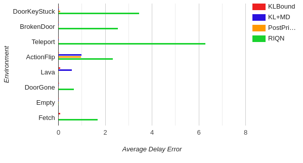
For functional novelty environments, all latent detection bounding techniques are effective at minimizing average delay error. Relying on the surrogate within the encoded latentrepresentation also seems to provide enough information to detect novelties with minimal delay error.

The CTMRE observational method could not detect functional novelties and are absent in Figure 4. Each of our techniques provide significant improvement of ADE over the RIQN method.

False Positives and False Negatives

We measure false positive and false negatives. Figure 5 shows the false positives of CTMRE and PP-MARE when operating in the novelty-free MiniGrid-Doorkey-6x6 environment. We hypothesize that the PP-MARE technique creates false positives in the beginning of the episode because the DreamerV2 RSSM cannot generate reasonable visuals due to the initial arbitrary $h_{0}$ encoding.

Figure 5: Percentage of transitions flagged as novelty within the original training environment, using observational based detection. We illustrate the errors of the CMTRE method using the random model threshold, trained agent threshold (as described in section Classical Multi-threshold Reconstruction Error), and Post Prior MARE using $\epsilon$ = 1.

Figure 6: Reconstruction error alongside the three tested thresholds: Random Model, Trained Model and Combination model (as described in section Classical Multi-threshold Reconstruction Error). Reconstruction error from the normal DoorKey-6x6 environment (Top), and Reconstruction error novel LavaGap environment (Bottom). Each vertical line refers to the cut off value for the corresponding threshold. Samples to the right of the line are classified as novelty. Reconstruction Error was generated from a trained agent.

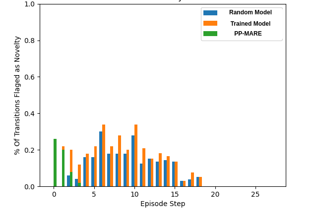
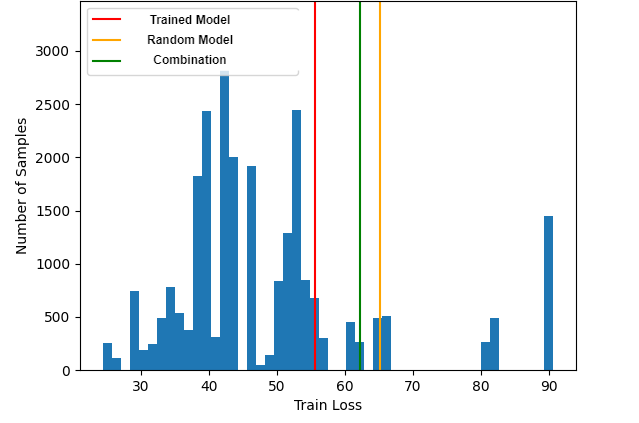
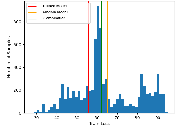
CTMRE incorrectly detects novelty within the first step of any episode at a lower false positive rate, but accumulates greater false positive as the episode progresses. The CTMRE method, however, also has high false negative and true positive thresholds, as shown in Figure 6.

Thus, if there is high likelihood that the agent experiences novelties with visual cues in the first steps of an episode, the CMTRE method is recommended. If visual cues are not likely to be immediately present, the PP-MARE visual detection method should be applied because PP-MARE tends to do better at minimizing false negatives in these environments but at the cost of an initially higher false positive rate. This tradeoff can be appealing if positives are likely to be an adversarial attack.

For functional novelties, Figure 7 shows the overall false positive rates. The KL method false positives rate is 0% and all techniques have dramatically lower false positive rates than RIQN. RIQN’s high false positive rate was also observed by Danesh and Fern (2021).

Figure 7: False alarm rates for each method captured during transitions within the original training environment.

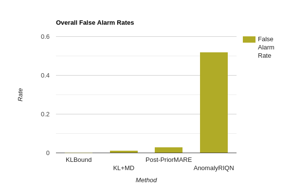
We initially witnessed high false positives rates by the KL+MD method during the first few steps of each episode. Similar to PP-MARE, early false positives result from the RSSM not having a valid representation given the arbitrary initial state $h_{0}$. To remedy this, we discovered that we could decrease the use of the Mahalanobis distance in the earlier step of an episode by setting $\lambda$ = $e^{-t/10}$ for each time step $t$, which account for the unreliable early representations.

While the KL+MD method has a higher false positive rate than the KL method, KL+MD typically yields a lower false negative rate (see Table 2 in the Appendix). This trade-off is to be expected because of the Mahalanobis distance added to the threshold.

Precision, Recall, Accuracy, and AUC

Table LABEL:table:AUCscores provide Area Under Curve (AUC) scores—capturing the trade-off between false positives and false-negatives—for different methods on different novelty-induced environments. Our latent methods (KL and KL+MD) have competitively higher AUC rates on all but one functional novelty environment. PP-MARE generally falls behind KL and KL+MD methods, likely partially due to the fact that the mean reconstruction error it is based on is not a measure optimized for computing differences between the observations. Further, PP-MARE assumes a false correlation between pixels with high reconstruction error and novel regions of input images (Feeney and Hughes 2021). In order to achieve a greater AUC for the PP-MARE method, a better similarity/difference metric should be used to quantify the differences between the observations.

For all specifics on precision, recall, and accuracy for cases when detection must continuously happen during the novel environment please refer to Table 2 in the appendix.

Table 1: AUC scores for all functional environments

Environment	KL	KL+MD	PPMARE	RIQN
DoorKeyStuck	.78	.89	.38	1
BrokenDoor	.939	.917	.7840	.92
Teleport	.9919	.99388	.959	.95
ActionFlip	.99121	.99315	.96299	.89

Conclusions

This paper proposed two types of bounding approaches for novelty detection in model based RL: (1) latent based methods which rely on the agent’s latent space encoding, and (2) observation based methods which rely on bounding the post and prior observation reconstruction error. Results on the Minigrid environments designed explicitly to introduce novelties that confound an agent confirm that these methods successfully detect novelties compared to traditional Machine learning and RL focused detection techniques.

We have learned that there exists ways to further utilize the learned world model transition distribution model to improve the debugging and safety performance for open-world environments, and believe that our methods can be used to formulate stronger bounds for the Bayesian surprise given different assumptions of the evaluation environment, as well as formulate other possible reactions once the novel transition is detected.

Based on the collective results across visual and functional novelties, we recommend coupling latent and observation based novelty detection methods, softening the detection votes of each method based on time step, when trying to minimize false positives and negatives.

Our paper supports the overall value of world model implementations and that world models provide a means for improved robustness, which is essential in open-worlds due to the possible degraded performance that can occur, before a reward signal is processed. We hope to advance and encourage further research in the field of novelty detection in reinforcement learning.

Table 2: Precision, Recall, Accuracy, and AUC for each environment.

	Metric	KLBound	KL+MD	PostPriorMARE	RIQN
BrokenDoor	Precision	.9908	.902	.916	.93277
	Recall	.63	.70	.62	.75778
	Accuracy	.811	.811	.7810	.73171
	AUC	.939	.917	.7840	.92
ActionFlip	Precision	.9999	.998	.994	.93277
	Recall	.975	.987	.983	.75778
	Accuracy	.9779	.9871	.9801	.63989
	AUC	.99121	.99315	.96299	.89
DoorKeyStuck	Precision	.707	.608	.023	.967
	Recall	.66	.99	.01	.704
	Accuracy	.79	.78	.50	.69
	AUC	.78	.89	.38	1
Teleport	Precision	.9998	.9990	.9957	.8526
	Recall	.955	.98	.97	.6011
	Accuracy	.95	.98	.97	.580441
	AUC	.9919	.99388	.959	.95
Lava	Precision	.84743	.870	.937	.7005
	Recall	.620	.784	.9119	.696
	Accuracy	.595	.713	.8718	.6319
	AUC	.732	.525	.765	.66
DoorGone	Precision	.971	.970	.973	.676
	Recall	.136	.3818	.395	.7004
	Accuracy	.39177	.56	.573	.607
	AUC	.940	.906	.685	.60
Empty	Precision	.603	.595	.6033	.585
	Recall	.954	.997	.9939	.643
	Accuracy	.599	.596	.607	.608
	AUC	.811	.639	.51721	.71
Fetch	Precision	1	1	.94	.6450
	Recall	.943	.99	.99	.744
	Accuracy	.97	.97	.97	.555
	AUC	1	1	.99	.50

Table 3: Custom environments

Environment	Description
BrokenDoor	The door no longer responds to the agent, regardless of key.
ActionFlip	Restrict the agent to left and right turns only.
Teleport	Teleport the agent randomly, then perform the selected action.
FakeGoal	The original goal is deactivated.
DoorKeyDiffColor	The color of the door and key changes.
DoorGone	The door is replaced with open space.
KeyStuck	The key can no longer be picked up.
Fetch	The agent’s goal is to collect various colored items in the environment.

References

- Asperti and Trentin (2020) Asperti, A.; and Trentin, M. 2020. Balancing reconstruction error and Kullback-Leibler divergence in Variational Autoencoders. arXiv:2002.07514.
- Åström (1965) Åström, K. J. 1965. Optimal control of Markov processes with incomplete state information. Journal of Mathematical Analysis and Applications, 10: 174–205.
- Balloch et al. (2022) Balloch, J.; Lin, Z.; Hussain, M.; Srinivas, A.; Wright, R.; Peng, X.; Kim, J.; and Riedl, M. 2022. NovGrid: A Flexible Grid World for Evaluating Agent Response to Novelty.
- Chevalier-Boisvert, Willems, and Pal (2018) Chevalier-Boisvert, M.; Willems, L.; and Pal, S. 2018. Minimalistic Gridworld Environment for Gymnasium.
- Cobbe et al. (2019) Cobbe, K.; Hesse, C.; Hilton, J.; and Schulman, J. 2019. Leveraging Procedural Generation to Benchmark Reinforcement Learning. CoRR, abs/1912.01588.
- Dabney et al. (2018) Dabney, W.; Ostrovski, G.; Silver, D.; and Munos, R. 2018. Implicit Quantile Networks for Distributional Reinforcement Learning.
- Danesh and Fern (2021) Danesh, M. H.; and Fern, A. 2021. Out-of-Distribution Dynamics Detection: RL-Relevant Benchmarks and Results. In International Conference on Machine Learning, Uncertainty & Robustness in Deep Learning Workshop.
- Dao and Lee (2019) Dao, G.; and Lee, M. 2019. Relevant Experiences in Replay Buffer. In 2019 IEEE Symposium Series on Computational Intelligence (SSCI), 94–101.
- Fang et al. (2022) Fang, Z.; Li, Y.; Lu, J.; Dong, J.; Han, B.; and Liu, F. 2022. Is Out-of-Distribution Detection Learnable? In Oh, A. H.; Agarwal, A.; Belgrave, D.; and Cho, K., eds., Advances in Neural Information Processing Systems.
- Feeney and Hughes (2021) Feeney, P.; and Hughes, M. C. 2021. Evaluating the Use of Reconstruction Error for Novelty Localization.
- Fu, Co-Reyes, and Levine (2017) Fu, J.; Co-Reyes, J. D.; and Levine, S. 2017. EX2: Exploration with Exemplar Models for Deep Reinforcement Learning. CoRR, abs/1703.01260.
- Gelada et al. (2019) Gelada, C.; Kumar, S.; Buckman, J.; Nachum, O.; and Bellemare, M. G. 2019. DeepMDP: Learning Continuous Latent Space Models for Representation Learning. CoRR, abs/1906.02736.
- Givan, Dean, and Greig (2003) Givan, R.; Dean, T.; and Greig, M. 2003. Equivalence notions and model minimization in Markov decision processes. Artificial Intelligence, 147(1): 163–223. Planning with Uncertainty and Incomplete Information.
- Greenberg and Mannor (2020) Greenberg, I.; and Mannor, S. 2020. Detecting Rewards Deterioration in Episodic Reinforcement Learning.
- Ha and Schmidhuber (2018) Ha, D.; and Schmidhuber, J. 2018. World Models. Interactive version of the article at https://worldmodels.github.io.
- Hafner et al. (2020) Hafner, D.; Lillicrap, T. P.; Norouzi, M.; and Ba, J. 2020. Mastering Atari with Discrete World Models. CoRR, abs/2010.02193.
- Itti and Baldi (2005) Itti, L.; and Baldi, P. 2005. Bayesian Surprise Attracts Human Attention. In Weiss, Y.; Schölkopf, B.; and Platt, J., eds., Advances in Neural Information Processing Systems, volume 18. MIT Press.
- Kiran et al. (2020) Kiran, B. R.; Sobh, I.; Talpaert, V.; Mannion, P.; Sallab, A. A. A.; Yogamani, S. K.; and Pérez, P. 2020. Deep Reinforcement Learning for Autonomous Driving: A Survey. CoRR, abs/2002.00444.
- Lee et al. (2018) Lee, K.; Lee, K.; Lee, H.; and Shin, J. 2018. A Simple Unified Framework for Detecting Out-of-Distribution Samples and Adversarial Attacks.
- Lee et al. (2019) Lee, K.; Lee, K.; Shin, J.; and Lee, H. 2019. A Simple Randomization Technique for Generalization in Deep Reinforcement Learning. CoRR, abs/1910.05396.
- Moerland et al. (2020) Moerland, T. M.; Broekens, J.; Plaat, A.; and Jonker, C. M. 2020. Model-based Reinforcement Learning: A Survey.
- Müller et al. (2022) Müller, R.; Illium, S.; Phan, T.; Haider, T.; and Linnhoff-Popien, C. 2022. Towards Anomaly Detection in Reinforcement Learning. In Proceedings of the 21st International Conference on Autonomous Agents and Multiagent Systems, AAMAS ’22, 1799–1803. Richland, SC: International Foundation for Autonomous Agents and Multiagent Systems. ISBN 9781450392136.
- Nguyen and Reddi (2021) Nguyen, T. T.; and Reddi, V. J. 2021. Deep Reinforcement Learning for Cyber Security. IEEE Transactions on Neural Networks and Learning Systems, 1–17.
- Page (1954) Page, E. S. 1954. Continuous Inspection Schemes. Biometrika, 41(1/2): 100–115.
- Pimentel et al. (2014) Pimentel, M. A. F.; Clifton, D. A.; Clifton, L. A.; and Tarassenko, L. 2014. A review of novelty detection. Signal Process., 99: 215–249.
- Robine, Uelwer, and Harmeling (2021) Robine, J.; Uelwer, T.; and Harmeling, S. 2021. Smaller World Models for Reinforcement Learning. arXiv:2010.05767.
- Ruan et al. (2015) Ruan, S. S.; Comanici, G.; Panangaden, P.; and Precup, D. 2015. Representation Discovery for MDPs Using Bisimulation Metrics. In Bonet, B.; and Koenig, S., eds., Proceedings of the Twenty-Ninth AAAI Conference on Artificial Intelligence, January 25-30, 2015, Austin, Texas, USA, 3578–3584. AAAI Press.
- Srivastava et al. (2014) Srivastava, N.; Hinton, G.; Krizhevsky, A.; Sutskever, I.; and Salakhutdinov, R. 2014. Dropout: A Simple Way to Prevent Neural Networks from Overfitting. Journal of Machine Learning Research, 15(56): 1929–1958.
- Wang et al. (2020) Wang, R.; Lehman, J.; Rawal, A.; Zhi, J.; Li, Y.; Clune, J.; and Stanley, K. O. 2020. Enhanced POET: Open-Ended Reinforcement Learning through Unbounded Invention of Learning Challenges and their Solutions. arXiv:2003.08536.
- Zhang, Goldstein, and Ranganath (2021) Zhang, L. H.; Goldstein, M.; and Ranganath, R. 2021. Understanding Failures in Out-of-Distribution Detection with Deep Generative Models. CoRR, abs/2107.06908.