SplitBeam: Effective and Efficient Beamforming in Wi-Fi Networks Through Split Computing

Abstract

Modern IEEE 802.11 (Wi-Fi) networks extensively rely on multiple-input multiple-output (MIMO) to significantly improve throughput. To correctly beamform MIMO transmissions, the access point needs to frequently acquire a beamforming matrix (BM) from each connected station. However, the size of the matrix grows with the number of antennas and subcarriers, resulting in an increasing amount of airtime overhead and computational load at the station. Conventional approaches come with either excessive computational load or loss of beamforming precision. For this reason, we propose SplitBeam, a new framework where we train a split deep neural network (DNN) to directly output the BM given the channel state information (CSI) matrix as input. The DNN is designed with an additional “bottleneck” layer to “split” the original DNN into a head model and a tail model, respectively executed by the station and the access point. The head model generates a compressed representation of the BM, which is then used by the AP to produce the BM using the tail model. We formulate and solve a bottleneck optimization problem (BOP) to keep computation, airtime overhead, and bit error rate (BER) below application requirements. We perform extensive experimental CSI collection with off-the-shelf Wi-Fi devices in two distinct environments and compare the performance of SplitBeam with the standard IEEE 802.11 algorithm for BM feedback and the state-of-the-art DNN-based approach LB-SciFi. Our experimental results show that SplitBeam reduces the beamforming feedback size and computational complexity by respectively up to 81% and 84% while maintaining BER within about $10^{-3}$ of existing approaches. We also implement the SplitBeam DNNs on FPGA hardware to estimate the end-to-end BM reporting delay, and show that the latter is less than 10 milliseconds in the most complex scenario, which is the target channel sounding frequency in realistic multi-user MIMO scenarios. To allow full reproducibility, we will release our code and datasets to the community.

I Introduction

Today, Wi-Fi networks are used to connect hundreds of millions of people worldwide. Wi-Fi is so ubiquitous that cellular operators are expected to offload 63% of their traffic to Wi-Fi by 2022 [1]. To attest to the need for higher data rates, the IEEE is currently standardizing 802.11be (Wi-Fi 7), which will support throughput of up to 46 Gbps through wider signal bandwidths and the usage of multi-user multiple-input and multiple-output (MU-MIMO) techniques [2]. MU-MIMO will become fundamental also to effectively decongest the unlicensed spectrum bands through spatial reuse, which are increasingly saturated [3]. To correctly beamform transmissions, MU-MIMO requires access points (APs) to periodically collect channel state information (CSI) from each connected station (STA) to beamform the transmissions [4, 5]. According to the IEEE 802.11 standard [6], the beamforming feedback (BF) is constructed by (i) measuring the CSI through pilot signals and (ii) computing the BF through singular value decomposition (SVD). Then, the BF is decomposed into Givens rotation (GR) angles that produce the beamforming matrix (BM), as explained in Section III-A.

A key challenge in MIMO systems is that the size of the BF grows with the number of subcarriers, transmitting and receiving antennas. For example, in an $8\times 8$ network at 160 MHz of bandwidth, the BF in 802.11 will be of size (486 subcarriers $\times$ 56 angles/subcarrier $\times$ 16 bits/angle =) 435,456 bits $\simeq$ 54.43 kB, if the maximum angle resolution is used. If BFs are sent back every 10 ms as suggested in [7], the airtime overhead is 435,456 / 0.01 $\simeq$ 43.55 Mbit/s. Moreover, the BF computation imposes a significant burden on the STAs, which may become intolerable for low-power devices. Specifically, the complexity of SVD and GR are $\mathcal{O}((4N_{t}N_{r}^{2}+22N_{t}^{3})\cdot S)$ and $\mathcal{O}(N_{t}^{3}N_{r}^{3}S)$, where $N_{t}$, $N_{r}$ and $S$ denote the number of transmitting and receiving antennas and subcarriers [8]. Since Wi-Fi 7 will support more spatial streams (up to 16) and bandwidth (up to 320 MHz), a thorough revision of how MIMO is performed in Wi-Fi is quintessential to keep the complexity under control.

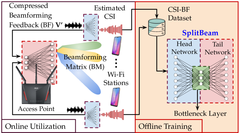
Fig. 1: High-level overview of the operations in SplitBeam.

Existing approaches to reduce MIMO complexity – discussed in details in Section II – come with excessive computation overhead and/or performance loss, with most of them not being compliant to the IEEE 802.11 standard [9, 10, 11, 12, 13, 14, 15, 16, 17, 18, 19, 20]. In this paper, we take a different approach and present SplitBeam, an IEEE 802.11 standard-compliant framework leveraging split computing to drastically decrease both computational load and BF size while maintaining reasonable beamforming accuracy. Figure 1 shows a high-level overview of SplitBeam. We first train a deep neural network (DNN) model to map the estimated CSI matrix to the BF in a supervised manner. Second, we “split” the DNN into a head and a tail model, respectively executed by the STAs and by the AP. The head model is custom-trained to produce a compressed representation of the BF through the introduction of a “bottleneck” inside the model, thus reducing BF airtime and STA computational load.

The key advantage of our approach is that the complexity of the head model and the BF representation size can be adjusted by modifying the bottleneck placement and size. Indeed, the bottleneck can trade off computational load, feedback size and beamforming accuracy, which was not available in previous approaches. This is crucial for constrained Wi-Fi devices and systems, which will cater to heterogeneous devices with different processing capacities [2].

This paper makes the following novel contributions:

$\bullet$ We propose SplitBeam, a novel framework for BF compression and STA computation reduction in MU-MIMO Wi-Fi networks. We perform a complexity analysis in Section IV-E and show that on average, SplitBeam successfully reduces the STA computational load and the BF size by respectively 92% and 91% when compared to the standardized 802.11 algorithm;

$\bullet$ We formulate a bottleneck optimization problem (BOP) to determine the bottleneck placement and size with the goal of minimizing airtime and computation overhead, while ensuring that the bit error rate (BER) and end-to-end delay are below the application’s desired level (Section IV-B). Given its complexity, we introduce a heuristic algorithm and propose a customized training procedure for the resulting DNN;

$\bullet$ We leverage off-the-shelf Wi-Fi equipment to collect CSI data in two different propagation environments, and compare the performance of SplitBeam with IEEE 802.11ac/ax CSI feedback algorithm [4, 5] (henceforth called 802.11 for brevity) and the state-of-the-art DNN-based compression technique, LB-SciFi [20]. Experimental results in Section VI show that the computational load and feedback size are reduced by up to 84% and 81% with respect to 802.11. Also, with the same compression rate, the computational load is reduced by up to 89% compared to LB-SciFi;

$\bullet$ We have synthesized SplitBeam in field-programmable gate array (FPGA) hardware by using a customized library to show the feasibility of SplitBeam in real-world Wi-Fi systems. Our experimental results show that the maximum end-to-end latency incurred by SplitBeam is less than 7 milliseconds (ms) in the case of $4\times 4$ MIMO operating at 160 MHz and lowest compression rate, which is well below the suggested threshold of 10ms in MU-MIMO Wi-Fi systems [7]. We pledge to release our code and our 230 GB dataset to the community for full reproducibility.

II Background and Related Work

In this section, we discuss prior work and highlight the novelty of this paper. We summarize CSI compression methods and data-driven feedback techniques in Section 2.1 and 2.2. CSI collection methodologies and current MU-MIMO CSI datasets are discussed in Section 2.3.

2.1: Traditional CSI Feedback Compression. Existing approaches can be categorized into (i) statistical approaches, (ii) compressive sensing (CS), and (iii) polar decomposition (PD) methods. The former methods leverage channel statistics to reduce the reporting frequency [9, 10, 11, 12]. As a consequence, their performance deteriorates in dynamic channel environments. Conversely, CS takes advantage of the sparsity of the channel response to compress the CSI. However, indoor channels might not be as sparse due to the presence of multiple reflectors. Moreover, many widely-used CS techniques such as BM3D-AMP [13] and OMP-US [14] experience slow convergence time. PD leverages the fact that the BF matrix is unitary. Thus, approaches such as Givens rotations (GR) can reduce the feedback size. However, computing and compressing the BF imposes an additional computational load. Subcarrier grouping, wide-band precoding [15] and reducing the number of feedback bits [6] can be used to decrease complexity, which come at the detriment of beamforming accuracy.

2.2: Data-Driven CSI Compression. Deep learning (DL) has been used for single-user MIMO (SU-MIMO) CSI compression [16, 17, 18, 19]. For instance, CS-ReNet [17], CsiNet[18], DeepCMC [19] have used convolutional neural network (CNN) and long short-term memory (LSTM) to extract the location of the significant time-domain channel taps by exploiting channel redundancy. However, the above work mostly assumes low-mobility, single-user, and outdoor Long-Term Evolution (LTE) scenarios, where channels responses are highly redundant and sparse due to the limited mobility and few local scatters at the base station (BS). In addition, conversely from SU-MIMO, inaccuracy in the beamforming will lead to inter-user interference (IUI) in MU-MIMO, which reduces the signal-to-interference-plus-noise ratio (SINR) significantly. Therefore, the CSI must be of higher resolution and more frequently updated. LB-SciFi [20] is the first deep learning (DL)-based work that investigated BF compression of an indoor wireless LAN (WLAN) network through adopting a autoencoder (AE)-based DNN. LB-SciFi model is composed of an encoder and a decoder. This model requires STAs to (i) compute the BF through SVD, (ii) decompose the BF into $\psi$ and $\phi$ angles using GR, and (iii) compress the angles using the encoder. At the AP, the received codes are decompressed using the decoder, and further inverse GR must be applied to recover the BF. Thus, the LB-SciFi’s encoder compounds the complexity of SVD and GR operations, which may exclude resource constraint devices. In addition, since the AE is trained for 20 MHz channels with 56 subcarriers, the growth rate of the encoder’s complexity with respect to the number of subcarriers is unknown. Conversely, in this work, we focus on reducing the computational load, as well as feedback airtime while maintaining the BER at an acceptable level. In Section VI, we show that while SplitBeam achieves the same level of feedback compression as LB-SciFi, it reduces the STAs’ computational load up to 89%.

2.3: CSI Collection and Datasets Availability. To the best of our knowledge, only a few Wi-Fi CSI datasets are publicly available, with the majority based on simulation data [17, 18, 19]. Authors in [20] collected MU-MIMO CSI dataset for training and evaluating the LB-SciFi. However, the experiment is limited to 20 MHz and the dataset is not publicly available. Although most commercial Wi-Fi chipsets can potentially generate CSI data, few manufacturers make this data available to developers and researchers, especially for modern chipsets such as 802.11ac/ax. Recently, the Nexmon firmware patch has been released, allowing the extraction of CSI from specific Broadcom/Cypress Wi-Fi chipsets [21]. To address the lack of large-scale MU-MIMO wireless dataset, for the first time, we collect a large-scale dataset containing multi-user (up to 3) multi-antenna (up to 3) fine-grained (up to 242 subcarriers) CSI data from multiple environments with different propagation characteristics using off-the-shelf Wi-Fi routers, which we will release to the community.

III Problem Statement and Challenges

In this section, we detail the BF acquisition procedure in WLAN 802.11 systems. Then, we discuss the challenges of applying such a technique to next-generation Wi-Fi systems.

III-A System Model and Preliminaries

In this section, we briefly introduce some terminology. We will adopt the following notation for mathematical expressions. We use boldface uppercase letters to denote matrices. We use the superscripts $T$ and ${\dagger}$ to denote the transpose and the complex conjugate transpose (i.e., the Hermitian). We define with $\angle{\mathbf{C}}$ the matrix containing the phases of the complex-valued matrix $\mathbf{C}$. Moreover, diag$(c_{1},\dots,c_{j})$ indicates the diagonal matrix with elements $(c_{1},\dots,c_{j})$ on the main diagonal. The $(c_{1},c_{2})$ entry of matrix $\mathbf{C}$ is defined by $\left[\mathbf{\mathbf{C}}\right]_{c_{1},c_{2}}$, while $\mathbb{I}_{c}$ refers to an identity matrix of size $c\times c$ and $\mathbb{I}_{c\times d}$ is a $c\times d$ generalized identity matrix. The notations $\mathbb{R}$ and $\mathbb{C}$ will indicate the set of real and complex numbers, respectively.

III-A1 WLAN MU-MIMO System Model

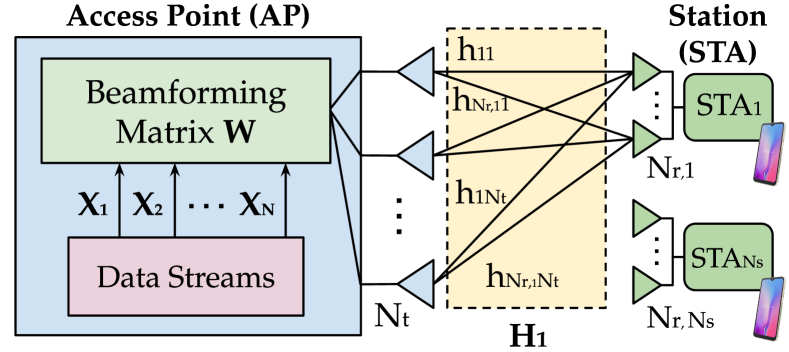
Fig. 2: Overview of a Wi-Fi MU-MIMO System.

We consider a MU-MIMO system with an AP as the beamformer, and a set $\mathcal{I}$ of $N_{s}$ STA devices as beamformees. The configuration of the MU-MIMO system is shown in Figure 2, where $N_{t}$ antennas are located at the AP and $N_{r,i}$ antennas are at each client. $N_{ss,i}$ is the number of spatial streams for STA $i$. Let $\mathbf{X}_{i}(s)\in\mathbb{C}^{N_{ss,i}\times 1}$ represent the transmitted data symbol vector for user $i$ over subcarrier $s\in\mathcal{S}$, where $\mathcal{S}$ is the set of $S$ orthogonal frequency-division multiplexing (OFDM) subcarriers. Each data symbol vector is beamformed through a beamforming matrix (BM) denoted by $\mathbf{W}_{i}(s)\in\mathbb{C}^{N_{t}\times N_{ss,i}}$. By defining the fading channel from the AP to STA $i$ as $\mathbf{H}_{i}(s)\in\mathbb{C}^{N_{r,i}\times N_{t}}$, the received signal at STA $i$ is

$$\mathbf{Y}_{i}=\sqrt{\frac{\rho}{N_{t}}}\hskip 2.84526pt\left(\mathbf{H}_{i}\mathbf{W}_{i}\mathbf{X}_{i}+\sum\limits_{\begin{subarray}{c}j\in\mathcal{I}\end{subarray}\setminus i}\mathbf{H}_{i}\mathbf{W}_{j}\mathbf{X}_{j}\right)+\mathbf{N}_{i},$$ (1)

where $\rho$ denotes the signal-to-noise-ratio (SNR) and is assumed equal for all users. $\mathbf{N}_{i}$ is the complex additive white Gaussian noise (AGWN) for STA $i$ as $\mathcal{CN}(0,1)$. To simplify notation, (1) is given in terms of the frequency domain for a single subcarrier and subcarrier index $(s)$ is omitted. We assume the number of transmit antennas is set to be the sum total of all the used spatial streams, $N_{t}=\sum_{i\in\mathcal{I}}N_{ss,i}$. The first term in (1) denotes the desired signal and the second term is the inter-user interference, which can be eliminated thanks to the beamforming. Ideally, $\mathbf{H}_{i}\mathbf{W}_{j}=0$ when $i\neq j$. Therefore, the received signal can be reduced to $\mathbf{Y}_{i}=\sqrt{\nicefrac{{\rho}}{{N_{t}}}}\mathbf{H}_{i}\mathbf{W}_{i}\mathbf{X}_{i}$.

III-A2 Computing the Beamforming Matrix

In MU-MIMO Wi-Fi systems, the beamforming matrix $\mathbf{W}$ with dimension $N_{t}\times\sum_{i=1}^{N_{s}}N_{ss,i}\times S$ is calculated using a multi-user channel sounding mechanism, shown in Figure 3. The procedure contains three main steps:

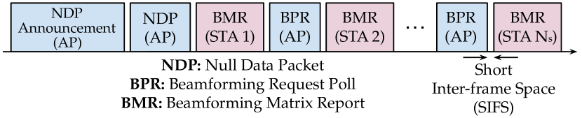
Fig. 3: Multi-user channel sounding procedure in IEEE 802.11.

(1) The AP begins the process by transmitting a null data packet (NDP) announcement frame, used to gain control of the channel and identify the STAs. The AP follows the NDP announcement frame with a NDP for each spatial stream;

(2) Upon reception of the NDP, each STA $i$ analyzes the NDP training fields – for example, VHT-LTF (Very High Throughput Legacy Training Field) in 802.11ac – and estimates the channel matrix $\mathbf{H}_{i}(s)$ for all subcarriers $s$, which is then decomposed by using SVD:

$$\mathbf{H}_{i}(s)=\mathbf{U}_{i}(s)\cdot\mathbf{S}_{i}(s)\cdot\mathbf{Z}_{i}(s)^{\dagger}$$ (2)

where $\mathbf{U}_{i}(s)\in\mathbb{C}^{N_{r,i}\times N_{r,i}}$ and $\mathbf{Z}_{i}(s)\in\mathbb{C}^{N_{t}\times N_{t}}$ are unitary matrices, while the singular values are collected in the $N_{r,i}\times N_{t}$ diagonal matrix $\mathbf{S}_{i}(s)$. With this notation, the complex-valued BM $\mathbf{V}_{i}(s)$ is defined by collecting the first $N_{ss,i}$ columns of $\mathbf{Z}_{i}(s)$. To simplify the notation, we will now drop the $i$ subscript and refer to a generic receiver. To reduce the channel overhead, $\mathbf{V}(s)$ is converted into polar coordinates as detailed in Algorithm 1. The output is matrices $\mathbf{D}_{s,t}$ and $\mathbf{G}_{s,\ell,t}$, defined as

$$\mathbf{D}_{s,t}=\begin{bmatrix}\mathbb{I}_{t-1}&0&\lx@intercol\hfil\dots\hfil\lx@intercol&0\\ 0&e^{j\phi_{s,t,t}}&0&\dots&\hbox{\multirowsetup\vdots}\\ \hbox{\multirowsetup\vdots}&0&\ddots&0&\\ &\vdots&0&e^{j\phi_{s,N_{t}-1,t}}&0\\ 0&\lx@intercol\hfil\dots\hfil\lx@intercol&0&1\end{bmatrix},$$ (3)

$$\mathbf{G}_{s,\ell,t}=\begin{bmatrix}\mathbb{I}_{t-1}&0&\lx@intercol\hfil\dots\hfil\lx@intercol&0\\ 0&\cos{\psi_{s,\ell,t}}&0&\sin{\psi_{s,\ell,t}}&\hbox{\multirowsetup\vdots}\\ \hbox{\multirowsetup\vdots}&0&\mathbb{I}_{\ell-t-1}&0&\\ &-\sin{\psi_{s,\ell,t}}&0&\cos{\psi_{s,\ell,t}}&0\\ 0&\lx@intercol\hfil\dots\hfil\lx@intercol&0&\mathbb{I}_{N_{r}-\ell}\end{bmatrix},$$ (4)

that allow rewriting $\mathbf{V}(s)$ as $\mathbf{V}(s)=\mathbf{\tilde{V}}(s)\cdot\mathbf{\tilde{D}}(s)$, with

$$\mathbf{\tilde{V}}(s)=\prod_{t=1}^{\min(N_{ss},N_{t}-1)}\Bigg{(}\mathbf{D}_{s,t}\prod_{l=t+1}^{N_{t}}\mathbf{G}_{s,l,t}^{T}\Bigg{)}\cdot\mathbb{I}_{N_{t}\times N_{ss}},$$ (5)

In the $\mathbf{\tilde{V}}(s)$ matrix, the last row – i.e., the feedback for the $N_{t}$-th transmitting antenna – consists of non-negative real numbers by construction. Using this transformation, the STA is only required to transmit the $\phi$ and $\psi$ angles to the AP. Moreover, it has been proved (see [6], Chapter 13) that the beamforming performance is equivalent when using $\mathbf{V}(s)$ or $\mathbf{\tilde{V}}(s)$. Thus, the feedback for $\mathbf{\tilde{D}}_{k}$ is not fed back to the AP.

Require: $\mathbf{V}(s)$;

$\mathbf{\tilde{D}}(s)={\rm diag}(e^{j\angle\left[\mathbf{V}(s)\right]_{N_{t},1}},\dots,e^{j\angle\left[\mathbf{V}(s)\right]_{N_{t},N_{ss}}})$ ;

$\mathbf{\Omega}(s)=\mathbf{V}(s)\cdot\mathbf{\tilde{D}}(s)^{\dagger}$;

for $t\leftarrow 1$ to $\min(N_{ss},N_{t}-1)$ do

      $\phi_{s,\ell,t}=\angle\left[\mathbf{\Omega}(s)\right]_{\ell,t}$ with $\ell={t,\dots,N_{t}-1}$;

      compute $\mathbf{D}_{s,t}$ through Equation (3);

      $\mathbf{\Omega}(s)\leftarrow\mathbf{D}_{s,t}^{\dagger}\cdot\mathbf{\Omega}(s)$;

      for $\ell\leftarrow t+1$ to $N_{t}$ do

           $\psi_{s,\ell,t}=\arccos\left(\frac{[\mathbf{\Omega}(s)]_{t,t}}{\sqrt{[\mathbf{\Omega}(s)]_{t,t}^{2}+[\mathbf{\Omega}(s)]_{\ell,t}^{2}}}\right)$;

           compute $\mathbf{G}_{s,\ell,t}$ through Equation (4);

           $\mathbf{\Omega}(s)\leftarrow\mathbf{G}_{s,\ell,t}\cdot\mathbf{\Omega}(s)$;

          

Algorithm 1 $\mathbf{V}(s)$ decomposition

(3) The AP transmits a beamforming report poll (BRP) frame to retrieve the angles from each STA. The angles are further quantized using $b_{\phi}\in\{7,9\}$ bits for $\phi$ and $b_{\psi}=b_{\phi}-2$ bits for $\psi$, to further reduce the channel occupancy. The quantized values – $q_{\phi}=\{0,\dots,2^{b_{\phi}}-1\}$ and $q_{\psi}=\{0,\dots,2^{b_{\psi}}-1\}$ – are packed into a compressed beamforming frame (CBF). Each contains $A$ number of angles for each of the $S$ OFDM sub-channels for a total of $S\cdot A$ angles each. For example, a $16\times 16$ system with 320 MHz channels requires 256 complex elements for each of the 996 subcarriers. The 802.11 standard requires 8 bits for each real and imaginary component of the CBF, which results in 510 kB.

III-B Challenges of 802.11 Beamforming Procedure

The size of the beamforming feedback (BF) grows as $N_{t}\times\sum_{i=1}^{N_{s}}N_{ss,i}\times S$. This implies the following drawbacks:

$\bullet$ Feedback airtime increases with the number of STAs, as each STA sends its BF separately. Moreover, the number of decomposed angles and ultimately the size of the BF depends on the number of antennas, and grows linearly with channel bandwidth, as discussed in Section IV-E2;

$\bullet$ Computing and compressing the through SVD and GR operations imposes a significant computational load on beamformees, as discussed in detail in Section IV-E1. This may impact resource-limited devices;

$\bullet$ GR angle decomposition and BF reconstruction introduce an additional error. This deteriorates the performance of the multi-user transmission, especially in scenarios with small inter-user separation where successful data recovery depends highly on accurate beamforming;

$\bullet$ The computational load at the STA and the feedback size cannot be modified according to application- and device-specific constraints. As next-generation Wi-Fi caters to heterogeneous devices and a wide range of performance requirements, it is critical to achieve this functionality.

IV The SplitBeam Framework

In this section, we elaborate on the SplitBeam framework. First, the system model and design challenges are outlined in Section IV-A. Next, the BOP is formulated and the heuristic solution is detailed in Sections IV-B and IV-C. Finally, the SplitBeam model implementation and the customized training procedure are explained in Section IV-D.

IV-A The SplitBeam DNN

SplitBeam trains a DNN that maps the CSI matrix $\mathbf{H}_{i}$ to the BF $\mathbf{V}_{i}$ in a supervised manner. To compress the BF and transfer the STAs computational load to the AP (with higher computational capacity), we introduce a “bottleneck layer” in the DNN as shown in Figure 4. The bottleneck is an intermediate representation in the DNN model which is ($K<1$ times) smaller than the model input $\mathbf{H}_{i}$. The bottleneck divides the DNN into a head and a tail network, which are respectively executed on the STA and the AP.

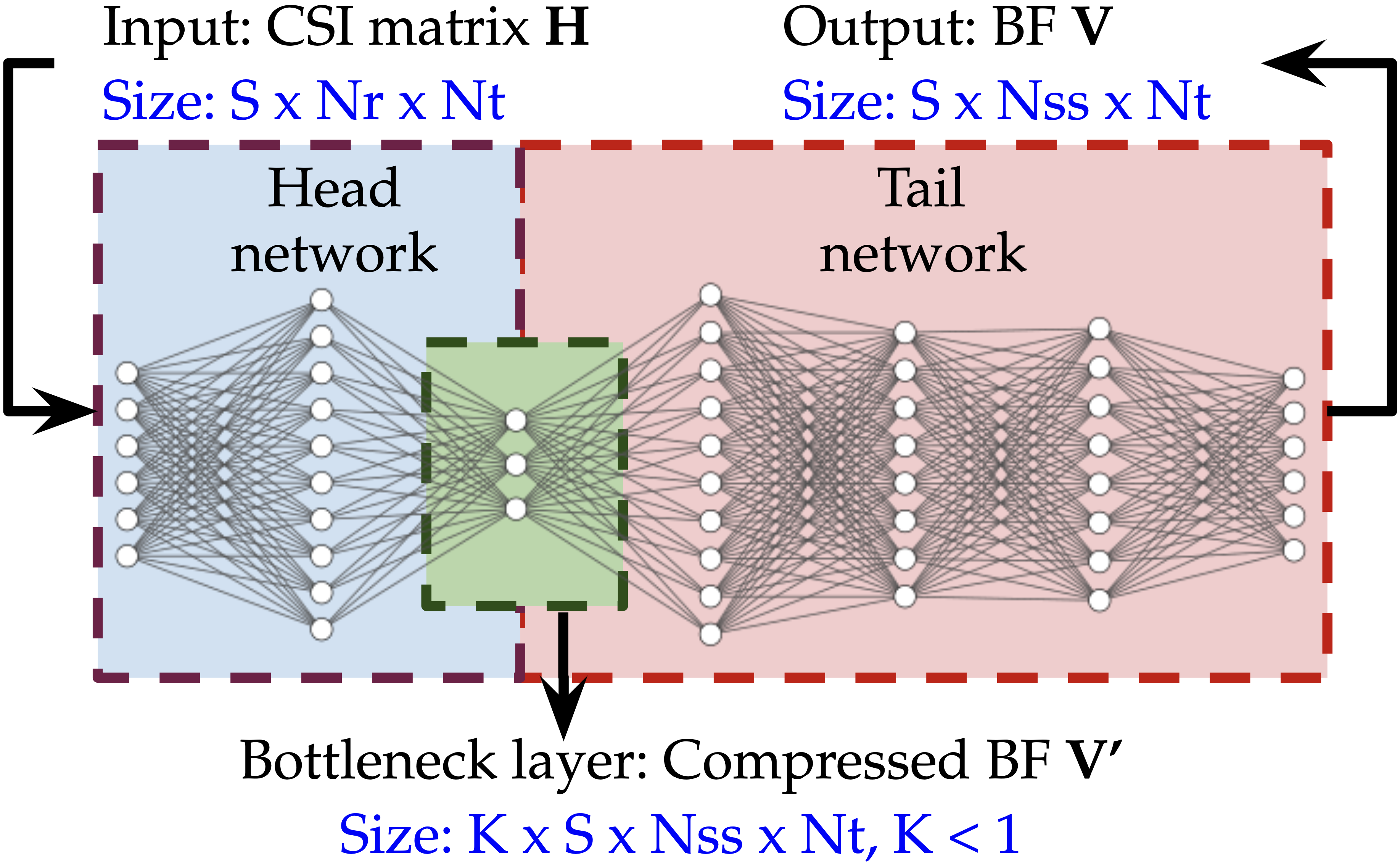
Fig. 4: Head and tail networks in SplitBeam. Notice that we dropped the index $i$ in the mathematical notation for simplicity.

An overview of SplitBeam is shown in Figure 5, where (1) the estimated CSI matrices at STAs are fed to the head model (2) that is tasked to produce a compressed representation of the BF denoted by $\mathbf{V}^{\prime}_{i}$ (3). The compressed BF is sent to the AP over the air (4), where it is fed to the tail model (5) to reconstruct the BF and generate the beamforming matrix(6).

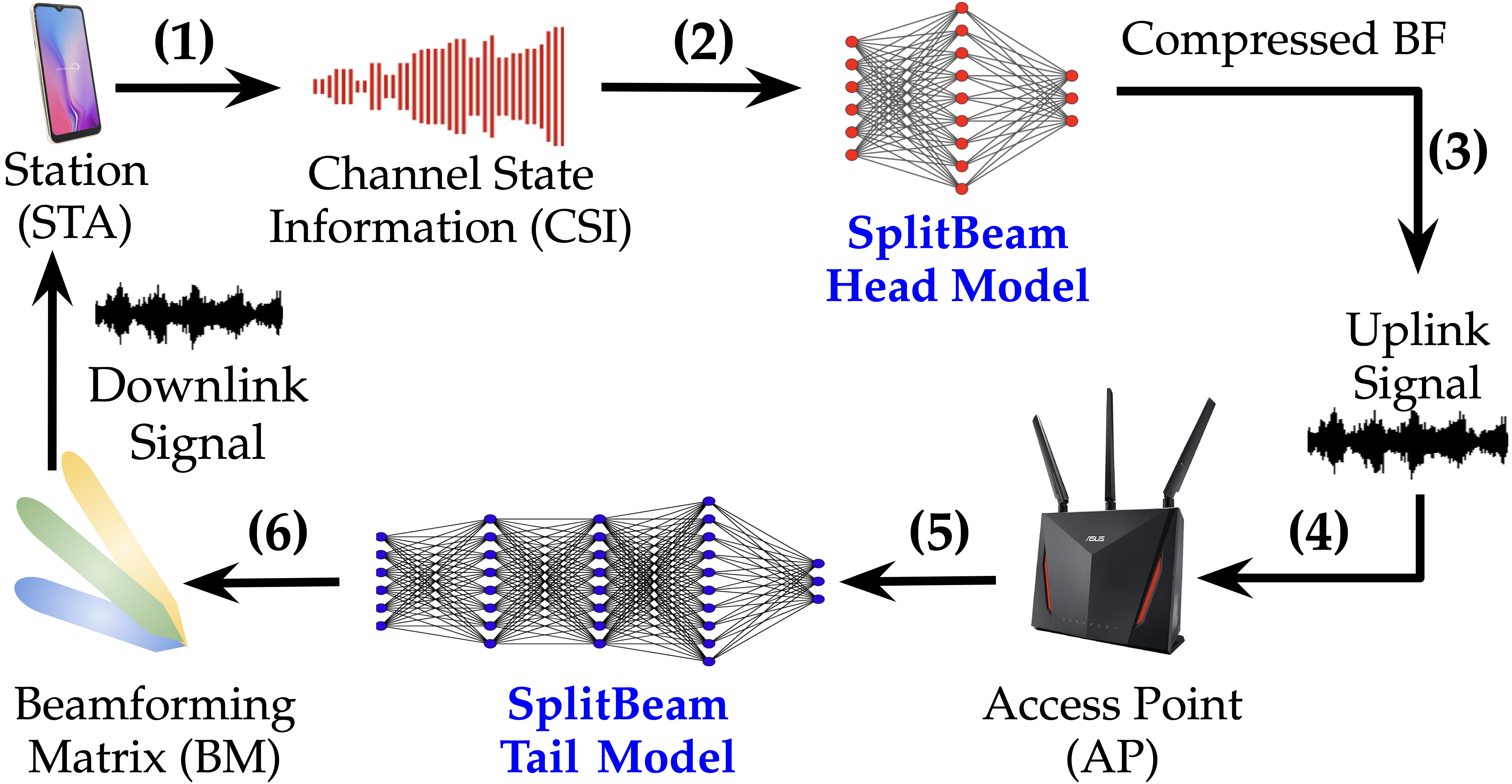
Fig. 5: SplitBeam beamforming feedback procedure.

Remarks. The placement and size of the bottleneck ultimately determine the head network architecture, and thus (i) the STA computational load, (ii) the BF feedback size, and (iii) the beamforming accuracy. Indeed, there is a trade-off between the complexity of the head model, the BF compression rate, and the accuracy of inference. While placing the bottleneck early on with a low number of nodes reduces the STA computation load and airtime overhead, it leads to a decrease in beamforming accuracy, which ultimately increases the BER. Therefore, the bottleneck placement and size must be adjusted according to the application-specific requirements.

IV-B Bottleneck Optimization Problem (BOP)

We model the original DNN as a function $\mathcal{M}$ that maps the channel matrix $\mathbf{H}_{i}\in\mathbb{C}^{N_{r}\times N_{t}\times S}$ to the BF $\mathbf{V}_{i}\in\mathbb{C}^{N_{r}\times N_{t}\times S}$ as $\mathcal{M}(\mathbf{H};\bm{\theta}):\mathbb{C}^{\mathbf{H}}\rightarrow\mathbb{C}^{\mathbf{V}}$, thorough $L$-layer transformations:

$$\mathbf{r}_{j}=F_{j}(\mathbf{r}_{j-1},\bm{\theta}_{j})\hskip 14.22636pt0\leq j\leq L,$$

where $F_{j}(\mathbf{r}_{j-1},\bm{\theta}_{j})$ is the mapping carried out by the $j$-th layer and $j=0$ denotes the input layer. The vector $\bm{\theta}=\{\bm{\theta}_{1},\ldots,\bm{\theta}_{L}\}$ defines the set of parameters of the DNN. To devise the bottleneck, we use an encoder-decoder like structure where the first $e$ layers of the DNN is the encoder and the rest of the layers are the decoder. The encoder, called the head model $\mathcal{H}$, is placed from the input layer to the bottleneck $\mathcal{B}$. Next, the tail model $\mathcal{T}$ decompresses the encoded BF to construct the BF $\mathbf{V}_{i}$. The modified model can be written as

$$\mathcal{M}(\mathbf{H};\bm{\theta})=\left\{\begin{array}[]{ll}\mathcal{H}=F_{j}(\mathbf{r}_{j-1},\bm{\theta}_{j})\text{,}&0\leq j<e,\\ \mathcal{B}=F_{e}(\mathbf{r}_{e-1},\bm{\theta}_{e})\text{,}&j=e,\\ \mathcal{T}=F_{j}(\mathbf{r}_{j-1},\bm{\theta}_{j}),&e+1\leq j\leq L.\end{array}\right.$$ (6)

Let $L_{i}^{\mathcal{H}}(e,N)$ be the STA $i$ overhead consists of three components: (i) the computational cost (i.e., the power consumption and memory required for executing the model), denoted by $L_{i}^{c}(e,N)$; (ii) the execution time for BF compression through the head model, denoted by $T_{i}^{\mathcal{H}}(e,N)$; and (iii) the power consumption of transmitting the compressed BF to the AP, denoted by $L_{i}^{tx}(e,N)$. Also, $T_{i}^{A}(e,N)$ represents the compressed BF feedback airtime. Finally, $T^{\mathcal{T}}(e,N)$ denotes the time required for reconstructing the BF at the AP. Notice that compression, decompression and airtime overhead depend on the placement $e$ and size of the bottleneck $N$.

We define the BOP such that it minimizes the STA computation overhead and feedback airtime as

$$\underset{e,N}{\min} \hskip 5.69046pt\sum_{i\in\mathcal{I}}\left(\mu_{i}^{\mathcal{H}}\hskip 2.84544ptL_{i}^{\mathcal{H}}(e,N)+(1-\mu_{i}^{\mathcal{H}})\cdot\hskip 2.84544ptT_{i}^{A}(e,N)\right)$$ (7a)

s. t. $$\hskip 5.69046pt0<\mu_{i}^{\mathcal{H}}<1,\hskip 5.69046pti\in\mathcal{I}$$ (7b)

$$\hskip 5.69046pt\mathrm{BER}_{i}\leq\gamma,\hskip 5.69046pti\in\mathcal{I}$$ (7c)

$$\hskip 5.69046pt\max_{i\in\mathcal{I}}(T_{i}^{\mathcal{H}}(e,N)+T^{A}_{i}(e,N))+T^{\mathcal{T}}(e,N)<\tau,$$ (7d)

where $\mu_{i}^{\mathcal{H}}$ parameterizes the importance of reducing the STAs overhead versus the feedback airtime. In applications where STAs are resource-constrained, it is crucial to reduce the STAs load, i.e., $\mu_{i}^{\mathcal{H}}>\mu_{i}^{A}$. On the other hand, in dynamic propagation environments like crowded rooms, where the channel coherence time is short, high feedback airtime cannot be tolerated. Thus, reducing the feedback airtime must be prioritized, i.e., $\mu_{i}^{\mathcal{H}}<\mu_{i}^{A}$. $\mathrm{BER}_{i}$ represents the bit error rate (BER) of client $i$. In this work, we measure the accuracy of the generated BF at the AP in terms of achievable BER by the STAs. BER is the number of erroneous bits divided by the total number of transferred bits. Condition (7c) guarantees that the BER experienced by each client does not exceed the maximum BER threshold $\gamma$. Condition (7d) indicates that the maximum end-to-end delay of BF cannot exceed the maximum tolerable delay denoted by $\tau$. In practice, these two conditions ensure that the bottleneck placement does not significantly impact the inference accuracy and latency. The maximum tolerable BER and delay can be specified according to the requirements.

IV-C Heuristic Procedure for Solving the BOP

The BOP is a particular instance of the extremely complex neural architecture search (NAS) problem [22, 23]. Thus, we devise a heuristic algorithm to search for proper SplitBeam hyperparameters that is specific to our context. Specifically, to limit the search space, we take the following procedure:

1. With the primary goal of minimizing the clients’ computational load $L_{i}^{\mathcal{H}}$, we place the bottleneck layer immediately after the input layer (i.e., $e=1$);

2. To reduce the inference time at the AP, $T^{\mathcal{H}}$, we consider only one layer for the tail network (i.e., $L=2$). Thus, the resulting DNN is a 3-layer network comprising input, bottleneck and output layers;

3. We adjust the size of the bottleneck layer according to the QoS requirements. Specifically, we consider a limited number of compression levels $K=\nicefrac{{\mathbf{V}^{\prime}_{i}}}{{\mathbf{H}_{i}}}$, and consider the BER as our QoS metric. We start from the highest level of compression (lowest number of bottleneck nodes), and train the 3-layer DNN with the CSI and corresponding $\mathbf{V}$ matrices dataset according to the customized procedure in Section IV-D. Once trained, the generated BM by the DNN is used to estimate the BER at the STA by comparing the recovered and transmitted data bits, as explained in Section 5.2.1.

4. If the desired BER cannot be achieved, the compression level is decreased. The new model is trained according to step (3) until the model is capable of meeting the BER constraint. If the compression level is the minimum, another layer is inserted after the bottleneck ($L=L+1$), and the algorithm goes back to step 3.

Section VI shows that the heuristic algorithm simplifies the search while maintaining acceptable performance.

IV-D SplitBeam Model Training

Since $\mathbf{H}$ and $\mathbf{V}$ are complex matrices, we decouple real and complex components in the matrices and treat them as double-sized real matrices. For each of our datasets, we split a dataset into training, validation, and test splits with 8:1:1 ratio. SplitBeam is trained offline for various network configurations and does not require retraining. The STAs select the proper trained DNN according to the network configuration information acquired from the NDP preamble.

IV-D1 Loss Function

Our goal is to deploy exactly the same model for each STA without fine-tuning its parameters to its environment. Notice that the training process is done offline (i.e., on a single computer). Given a channel matrix $\mathbf{H}_{i}$, our DNN model $\mathcal{M}$ estimates the corresponding BF $\mathbf{V}_{i}$, i.e., $\mathbf{V}_{i}=\mathcal{M}(\mathbf{H}_{i},\bm{\theta})$. We formulate the loss function $\mathcal{L}$ as follows

$$\mathcal{L}=\frac{1}{b}\sum_{j=1}^{b}\sum_{i=1}^{N_{s}}\frac{\left(\mathcal{M}(\mathbf{H}_{i}^{j},\bm{\theta})-\mathbf{V}_{i}^{j}\right)^{2}}{\left\|\mathbf{V}_{i}^{j}\right\|_{1}},$$ (8)

where $b$ indicates training batch size and $\|\cdot\|_{1}$ represents L1-norm. $\mathbf{H}_{i}^{j}$ and $\mathbf{V}_{i}^{j}$ indicate the $j$-th channel matrix and BF for STA $i$, respectively. By minimizing the loss in (8), we optimize the parameters $\bm{\theta}$ of our DNN model $\mathcal{M}$. We use stochastic gradient descent (SGD) and Adam [24] to train the synthetic and experimental datasets, respectively. Unless specified, we train models for 40 epochs, using the training split in the dataset with batch size of 16 and the initial learning rate of $10^{-3}$. The learning rate is decreased by a factor of 10 after the end of 20th and 30th epochs. Using the validation split in the dataset, we assess the model in terms of achieved BER at the end of every epoch and save the best parameters $\bm{\theta}^{*}$ such that achieve the lowest BER for the validation split. The trained model is assessed with the best parameters for the held-out test split in the dataset and report the test BER.

IV-D2 Difference with Autoencoders

Although an AE is similar in terms of model architecture, its training objective is different. AEs are trained to reconstruct its input in an unsupervised manner (e.g., to estimate $\hat{\mathbf{V}}_{i}$ given $\mathbf{V}_{i}$) as done in [20]. Conversely, we train a task-specific model in a supervised fashion to estimate BF $\mathbf{V}_{i}$ given a channel matrix $\mathbf{H}_{i}$.

IV-E Complexity Analysis and Compression Rate

IV-E1 Computational Overhead

The complexity of the SVD operation for decomposing the BF $\mathbf{V}$ in 802.11 is $\mathcal{O}((4N_{t}N_{r}^{2}+22N_{t}^{3})S)$, according to [8]. The BF is further transformed into a set of angles using the Givens rotation (GR) matrix multiplication which has a complexity of $\mathcal{O}(N_{t}^{3}N_{r}^{3}S)$ [6]. Conversely, the complexity of SplitBeam is $\mathcal{O}(KN_{t}^{2}N_{r}^{2}S^{2})$, where $K<1$ denotes the head model’s compression level.

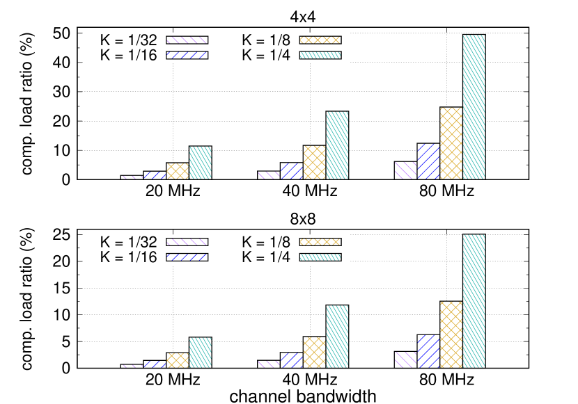
Fig. 6: The ratio of the computational load using SplitBeam to 802.11 with $N_{ss,i}=1$ and various compression levels $K$ and channel widths.

Figure 6 shows the ratio of the number of floating-point operations (FLOP) required for compressing the BF using SplitBeam to 802.11 compression technique. The ratio is calculated by $\nicefrac{{X}}{{Y}}\times 100$ where $X$ and $Y$ denote the number of floating points operation in SplitBeam and legacy Wi-Fi protocol, respectively. The comparison is performed for different MU-MIMO orders and a various number of subcarriers, as computed through a MATLAB program. We can see that SplitBeam noticeably reduces the computational load of STA, especially as the number of antennas and/or STAs increases. At 80 MHz, SplitBeam with $K=\nicefrac{{1}}{{8}}$ decreases 75% and 87% of the STA’s load in $4\times 4$ and $8\times 8$ systems. On average, SplitBeam improves computation by 73%. We show in Section VI that SplitBeam with $K=\nicefrac{{1}}{{8}}$ keeps the BER within 87% of 802.11.

IV-E2 Airtime Overhead

In 802.11, the size of the compressed BF report is $BMR=8\times N_{t}+N_{a}\times S\times(b_{\phi}+b_{\psi})/2$ where $N_{a}$ denotes the number of Givens angles [6]. Notice that $b_{\phi}$ and $b_{\psi}$ are the number of bits required for the angle quantization [7]. Therefore, the 802.11 compression ratio can be written as

$$CR=\frac{BMR}{S\times N_{t}\times N_{r}\times b}\vspace{3pt},$$ (9)

where $b=16$ is the number of bits required for transmitting channel information over each subcarrier. Conversely, the compression rate of SplitBeam is $K$. Notice that it is constant and does not grow with the size of the channel matrix.

Figure 7 depicts the impact of SplitBeam in reducing the airtime overhead. The bars show the ratio of the size of the compressed BF of SplitBeam to the angle decomposition technique in 802.11. SplitBeam has a significant impact at higher-order MU-MIMO configurations. For example, SplitBeam reduces the size of the feedback overhead by 91% and 93% in $4\times 4$ and $8\times 8$ configurations with 80 MHz channel. On average, SplitBeam reduces the airtime overhead by 75% with respect to 802.11.

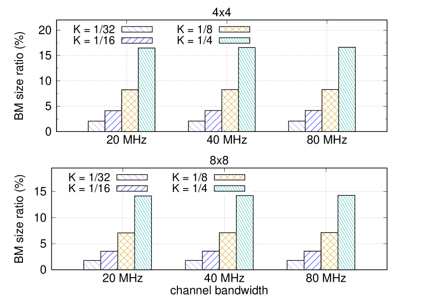
Fig. 7: The ratio of the size of BF using SplitBeam to 802.11 with $N_{ss,i}=1$ and various compression levels $K$ and channel widths.

V Experimental Evaluation

We first introduce the experimental MU-MIMO CSI extraction method along with the measurement campaigns for building the datasets in Section V-A. Next, we detail organization of the dataset, the training and testing procedure of the SplitBeam using the collected datasets in Section V-B.

V-A Experimental Setup

We designed our testbed with commercially-available off-the-shelf Wi-Fi devices to collect real-world datasets. As explained in Section IV-D, training the SplitBeam requires downlink CSI that is measured at the STA side, in addition to the corresponding BF. The measurements are carried over different network configurations to verify the performance of SplitBeam as the number of subcarriers and antennas and STAs increases. We consider different propagation environments to test how SplitBeam generalizes.

5.1.1: CSI Extraction. In commercial Wi-Fi chipsets, CSI data is estimated through pilot symbols. Being computed at the physical layer (PHY), CSI is not accessible by the end-user through normal network interface cards (NICs). Thus, we have used Nexmon CSI [21], the state-of-the-art CSI extraction tool to collect CSI measurements using Asus RT-AC86U 802.11ac Wi-Fi routers as STAs. The extraction tool is compatible with the very-high-throughput (VHT) mode, defined by IEEE 802.11ac, working with bandwidth up to 80 MHz. Each CSI sample results in complex-valued channel information per subcarrier for each transmit-receive antennas pair. A Netgear R7800 Wi-Fi router with a Qualcomm Atheros chipset is used as AP. An example of the experimental setup realization is shown in Figure 8(b). In a real-world scenario, SplitBeam relies on already existing channel estimations at the STAs. However, since the Nexmon tool is configured for reading CSI samples only on data packets, we established a Wi-Fi link between the AP and another Netgear R7800 Wi-Fi router (as the client) to generate the data packets that provides the ASUS STAs the opportunity to extract CSI.

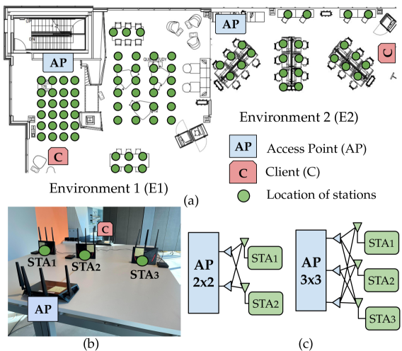
Fig. 8: Experimental setup for MU-MIMO CSI data collection: (a) different environments; (b) network elements; (c) network configurations.

V-B Data Collection and Model Training

Packets are transmitted with a rate of 1000 packets/second through $N_{t}$ antennas with a fixed modulation and coding scheme. Thus, a new CSI is generated every $T=10^{-3}$ s. To evaluate the capability of SplitBeam in generalizing to different environments, we performed CSI measurements in two environments $E1$ and $E2$. We carefully picked the environment with exclusive furniture arrangements, size, and construction material to ensure that the target environments are mutually exclusive from the source environment in terms of propagation characteristics. Specifically, $E1$ has fewer reflectors and human traffic, while $E2$ is furnished with more furniture (multipath) and is imposed to higher human traffic. Figure 8(a) displays the positions of the AP and STAs in the different environments. To capture the impact of inter-user distance on CSI data, the STAs are placed in different distances from each other (15-60 cm). Also, users are located at different distances from the AP (0.5-6 m). The green dots in Figure 8(a) depicts the location of points where STAs are located for data collection.

5.2.1: Datasets.  We consider $2\times 2$ and $3\times 3$ scenarios, where the AP with $N_{t}=2,3$ antennas simultaneously serves two and three STAs. The network configurations are shown in Figure 8(c), where each STA device supports one spatial stream, i.e., $N_{ss,i}=1$ for $i\in\mathcal{I}$. Moreover, the Nexmon tool enabled us to collect 802.11ac channel measurements at 5 GHz with 20, 40 and 80 MHz bandwidth over $|\mathcal{S}|=56$, $|\mathcal{S}|=114$ and $|\mathcal{S}|=242$ subcarriers, to assess the performance of the SplitBeam at higher channel bandwidth. The measurements are repeated several times with a time interval of at least 4 hours in between measurements. To capture the impact of human blockage and reflection, the datasets are collected during working and non-working days. We collected 10,000 CSI samples per configuration, channel width and environment. In total, 12 datasets with 120,000 data samples were extracted to train, evaluate and test the SplitBeam. Tables I shows the list of collected experimental datasets. We pledge to release, along with the code, the collected dataset for full reproducibility.

			Config.
Type	BW (MHz)	Env.	$2\times 2$	$3\times 3$	$4\times 4$
		$E1$	$\mathcal{D}_{1}$	$\mathcal{D}_{2}$	-
	20	$E2$	$\mathcal{D}_{3}$	$\mathcal{D}_{4}$	-
		$E1$	$\mathcal{D}_{5}$	$\mathcal{D}_{6}$	-
	40	$E2$	$\mathcal{D}_{7}$	$\mathcal{D}_{8}$	-
		$E1$	$\mathcal{D}_{9}$	$\mathcal{D}_{10}$	-
Real	80	$E2$	$\mathcal{D}_{11}$	$\mathcal{D}_{12}$	-
Synth.	160	MATLAB	$\mathcal{D}_{13}$	$\mathcal{D}_{14}$	$\mathcal{D}_{15}$

TABLE I: Datasets collected during our data collection campaign.

We have used the MATLAB WLAN toolbox to generate a dataset at 160 MHz. This is because our experimental setup did not allow us to collect CSI at 160 MHz and with $4\times 4$ MIMO. We have used wlanTGacChannel function that filters an input signal through an 802.11ac multipath fading channel. The multi-user channel consists of independent single-user MIMO channels between the AP and spatially separated stations. Each user estimates its own channel using the received NDP signal and computes the CSI. The delay profile “Model-B” has been considered which respectively consists of 9 channel taps and 2 channel clusters. Dataset $\mathcal{D}_{13}$-$\mathcal{D}_{15}$ each contain 10,000 data points. To remove noise and unwanted amplification, the CSI elements are normalized by the mean amplitude over all subcarriers. In addition, to remove the noise a $n$-point moving median window with $n=10$ is used to smooth out the noisy data. In addition, we noticed that in some instances, CSI packets are dropped by some STAs. Therefore, using the packets sequence number, the data collected from different devices are aligned to ensure that each CSI element collected over different STAs represents the same time and frequency domain channel measurements for seamless beamforming.

5.2.2: BER Computation. A key issue is that BER extremely depends on noise and fading levels, which makes it challenging to isolate the BER caused by the DNN compression. For this reason, and the sake of repeatability, we have used a MATLAB-based program to compute the BER corresponding to a given DNN compression. We have set the total number of transmit antennas to the sum of all the used spatial streams, so that no space-time block coding (STBC) or spatial expansion is needed at the AP. Moreover, no channel coding is considered, unless otherwise specified. The BER measurement procedure for each collected CSI data point $j$ is as follows: (1) we randomly generate bits modulated with 16-QAM that are used as payload to generate $N_{s}$ standard-compliant 802.11 frames $\mathbf{F}^{j}=[\mathbf{F}^{j}_{1}\cdots\mathbf{F}^{j}_{N_{s}}$] for $N_{s}$ receiving STA each served with one spatial stream. Denoting the $j$-th CSI value collected from the $i$-th STA as $\mathbf{H}_{i}^{j}$, (2) we run the SplitBeam trained head and tail models $\mathcal{M}_{i}$ for each user to compute the $\mathbf{V}_{i}^{j}$ values corresponding to the $\mathbf{H}_{i}^{j}$ inputs; (3) we compute $\mathbf{H}_{\text{EQ}}^{j}=[\mathbf{V}_{1}^{j},\cdots,\mathbf{V}_{N_{s}}^{j}]$ as described in Section III-A2; (4) we use zero-forcing (ZF) beamforming to calculate $\mathbf{W}^{j}$ as

$$\mathbf{W}^{j}=\mathbf{H}_{EQ}^{j}\cdot(\mathbf{H}^{j\dagger}_{EQ}\cdot\mathbf{H}_{EQ}^{j})^{-1}.$$

(5) The received packets are generated as $\mathbf{Y}^{j}=\mathbf{H}_{i}^{j}\hskip 3.0pt\mathbf{W}_{i}^{j}\hskip 3.0pt\mathbf{F}_{i}^{j}+\mathbf{N}_{i}$, where $\mathbf{N}_{i}$ is Gaussian white noise. Finally, (6) the packets are demodulated, and the recovered bits are compared with the transmitted bits to calculate the BER.

5.2.3: Model Training and Testing. For each CSI measurement dataset in Table I the corresponding BF dataset is generated using SVD. Next, SplitBeam is trained to map the CSI measurement to BF in a supervised manner, as detailed in Section IV-D. We used $K=\nicefrac{{1}}{{32}}$, $\nicefrac{{1}}{{16}}$, $\nicefrac{{1}}{{8}}$, and $\nicefrac{{1}}{{4}}$ as compression levels. A model is trained for each scenario, by using 80% and 10% of each dataset for training and validation. We designed two testing procedures: (i) single-environment test, where the trained model is tested on the remaining 10% of its dataset; (ii) cross-environment test, where the model is tested on its counterpart dataset from the other environment. For example, let $\mathcal{M}_{1}$ be the model that is trained with $\mathcal{D}_{1}$ which is a $2\times 2$ dataset collected in $E1$ at 20 MHz channel width. The model $\mathcal{M}_{1}$ is tested on: (i) $\mathcal{D}_{1}$ test-split that was held out during the training; (ii) $\mathcal{D}_{3}$ which is the dataset with the same configuration and channel width in $E2$.

VI Experimental Results

We first compare the compression rate of SplitBeam with respect to 802.11 and state-of-the-art LB-SciFi [20] in Section VI-A. LB-SciFi uses an autoencoder (AE) to compress the angles generated by the 802.11 BF compression algorithm. Finally, we evaluate the SplitBeam generalization and efficiency results in Section VI-B.

VI-A Comparison with 802.11 and LB-SciFi

Figure 9 depicts the trade-off between BF compression rate ($K=\mathbf{V}^{\prime}/\mathbf{H}$) and the incurred BER with respect to 802.11. It can be seen that as the compression rate decreases and the BF gets more compressed, the BER increases. However, we observe that the size of the feedback is much higher in 802.11. It can be seen that the SplitBeam with a compression rate of $K=\frac{1}{8}$ achieves a BER close to – in some instances lower than – the legacy Wi-Fi protocol while its size of BF is respectively 4 and 5 times smaller in $2\times 2$ and $3\times 3$ configurations.

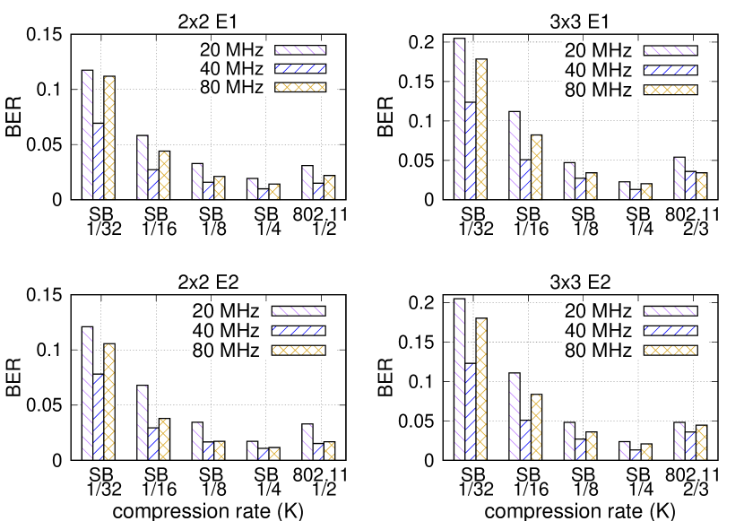
Fig. 9: BER as a function of compression rate ($K=V^{\prime}/H$): SplitBeam (SB) vs 802.11; $2\times 2$ and $3\times 3$ MU-MIMO configurations in $E1$ and $E2$. Notice that in IEEE 802.11 $K\simeq 1/2$ and $2/3$ in $2\times 2$ and $3\times 3$ configurations as the compression rate depends on network parameters as Equation (9).

Figure 10 shows achievable BER and computational load, in terms of number of floating point operations (FLOP), for 160 MHz Wi-Fi transmissions (datasets $\mathcal{D}_{13}$ – $\mathcal{D}_{15}$). For these results, we used binary convolutional coding (BCC) with a code rate of 1/2. SplitBeam achieves BER close to legacy 802.11 standard and LB-SciFi, which is the desired level. However, both 802.11 and LB-SciFi require SVD and GR operations that impose high computational load on clients to achieve this performance. Figure 10 shows that SplitBeam reduces the computational load by 65% and 45% with respect to 802.11 and LB-SciFi as it directly compresses the CSI matrix. When SplitBeam is combined with channel coding, the BER is reduced significantly. Moreover, higher MU-MIMO orders are more sensitive to BM estimation error.

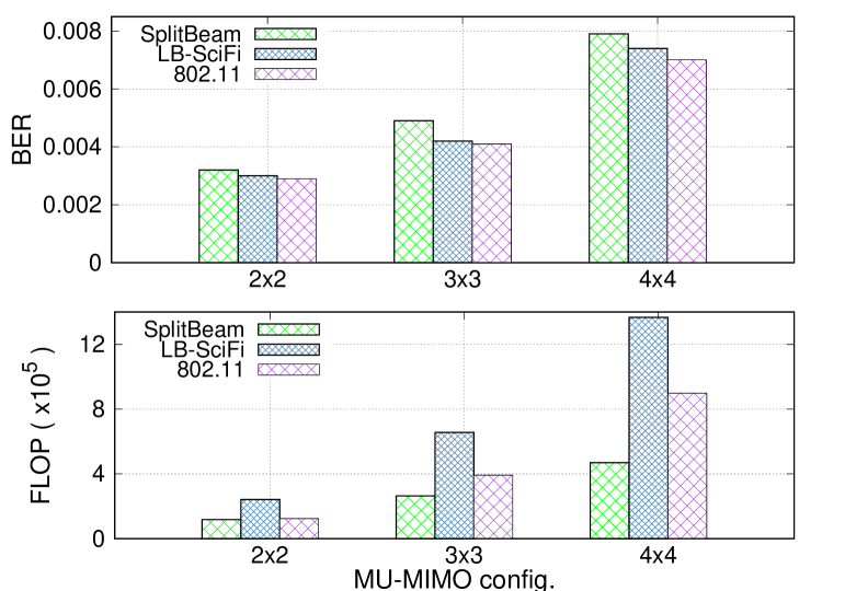
Fig. 10: BER and STAs computational load for synthetic datasets with 160 MHz channel and compression rate of $K=\frac{1}{8}$.

Figure 11 compares the achievable BER of the SplitBeam with 802.11 protocol as a function of computational load. We observe that SplitBeam maintains the BER of the STA close to the 802.11 protocol while imposing a considerably lower computational load on the users. Specifically, SplitBeam decreases the computation load by 70% with respect to 802.11 while maintaining the same BER value of 0.02. We notice that the improvement given by SplitBeam is more prominent when the number of antennas increases. For instance, SplitBeam with $K=\frac{1}{8}$ decreases STAs’ computational load respectively by 52% and 68% for $2\times 2$ and $3\times 3$ MU-MIMO.

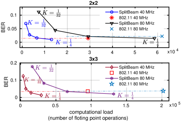
Fig. 11: BER as a function of computational STAs computational load: SplitBeam vs 802.11; for $2\times 2$ and $3\times 3$ MU-MIMO configurations.

VI-B Model Generalization and Efficiency

Figure 12 shows the BER and computational complexity for $3\times 3$ MU-MIMO configuration with 80 MHz channel bandwidth in different environments. In the cross-environment setting $E1/E2$ ($E2/E1$), the models are trained and validated with the data collected from $E1$ ($E2$) and tested with the data from $E2$ ($E1$). Although LB-SciFi achieves the same level of compression and BER as SplitBeam (slightly lower in some cases), its computational load on STAs is much higher than SplitBeam. Specifically, on average, SplitBeam improves the computational load by 78% with respect to LB-SciFi, while maintaining similar BER. This is since our approach compresses the estimated channel directly thus offloading devices’ overhead significantly. Figure 13 further depicts the capability of SplitBeam to generalize to untrained environments. We observe that in most cases, the cross-environment test has a performance close to the single-environment test. Interestingly, we observe that the BER is usually lower when models are trained in $E2$ and tested in $E1$. This is because $E2$ has a more complex propagation profile than $E1$, i.e., more reflectors and presence of people. Thus, $E2$-trained models are more comprehensive and thus generalizing better.

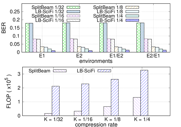
Fig. 12: BER and computational load for SplitBeam vs LB-SciFi; single- and cross-environment test for $3\times 3$ MU-MIMO with 80 MHz channel widths. Notice that BER is shown for $K=\frac{1}{8}.$

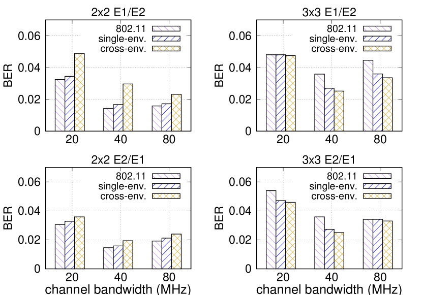
Fig. 13: Cross-environment test: BER for $3\times 3$ and $2\times 2$ MU-MIMO configurations with compression rate of $K=\frac{1}{8}$. Note that $X/Y$ indicates that the model is trained in $X$ and tested in $Y$.

Table II investigates the trade-off among the head model complexity, the size of the BF, and BER, as a function of the bottleneck structure in a $2\times 2$ MIMO network. We compare the performance of the 3-layer DNN– designed and trained using the procedure explained in IV-C – with more complex DNNs with a higher number of hidden layers and neurons. We notice that the BER decreases as the size of the bottleneck and the depth of the head model increases. This performance enhancement, however, comes to the detriment of computational load and feedback overhead.

BW (MHz)	Full Model	$\bm{|\mathcal{B}|}$	BER
	224-28-28-224	28	0.0342
	224-896-1792-1792-896-224	1792	0.0077
20	224-896-896-448-448-224-224	448	0.015
	456-57-57-456	57	0.0158
	456-1824-3648-3648-1824-456	3648	0.0053
40	456-1824-1824-912-912-456-456	912	0.0083
	968-121-121-968	121	0.0172
	968-3872-7748-7748-3872-968	7748	0.017
80	968-3872-3872-1936-1936-968-968	1936	0.0202

TABLE II: Impact of the bottleneck placement and size ($\bm{|\mathcal{B}|}$) on BER, size of BF and STAs’ computational load. The head model parameters are boldfaced. The highlighted rows are the 3-layer SplitBeam with $K=\nicefrac{{1}}{{8}}$.

On the other hand, increasing the model parameters does not guarantee to improve the accuracy of the predictions. For example, for $2\times 2$ at 20 MHz, the head model with multiply-accumulate (MAC) of 6,641,152 results in a BER of 0.0182 while a model with MAC of 1,612,800 (75% less computational load) has a lower BER of 0.015. This is due to the model severely overfitting the training data. The results demonstrate that heuristic algorithm simplifies the search process while maintaining acceptable performance, within about $10^{-3}$ of existing approaches.

	Signal Bandwidth
MIMO	20 MHz	40 MHz	80 MHz	160 MHz
$2\times 2$	0.0202ms	0.0824ms	0.3686ms	1.477ms
$3\times 3$	0.0459ms	0.1867ms	0.8337ms	3.314ms
$4\times 4$	0.0808ms	0.3298ms	1.4782ms	5.883ms

TABLE III: SplitBeam latency vs MIMO dimensions and bandwidth size.

Latency Analysis with FPGA Synthesis. While it is sufficient to perform MIMO channel sounding once every 100ms, MU-MIMO channel sounding should be performed at least once every 10ms to account for user mobility, according to [7] (see page 73). This implies that keeping the end-to-end BM computation within 10ms latency is fundamental. To this end, we have synthesized in FPGA the neural networks implemented by SplitBeam. We evaluated the latency with up to 160 MHz, which is the maximum as per the 802.11ax standard, and with MIMO dimensionality up to $4\times 4$. We considered $K=\nicefrac{{1}}{{4}}$ compression rate, which results in the lowest BER value as shown in Figure 9.

As target device, we chose a Zynq UltraScale+ XCZU9EG-2FFVB1156, a commonly used System-on-Chip for software-defined radios that is also supported by the OpenWiFi project as part of the ZCU102 evaluation board [25]. We chose 5ns as clock period (200 MHz clock frequency), which is the operating clock of the AD9361 transceiver [26] used in OpenWiFi. We have used a customized library based on high-level synthesis (HLS) designed by us to synthesize the neural networks. HLS allows the conversion of a C++-level description of the DNN directly into hardware description language (HDL) code such as Verilog. Therefore, improved latency results could be achieved with more advanced synthesis strategies. Moreover, better latency results could be achieved by utilizing application-specific integrated circuits (ASICs), which however allow little room for reconfigurability.

Table III shows the results obtained through our FPGA synthesis process described above. We notice that by doubling the bandwidth, the latency of the design increases by about 4 times on the average, which is also true when MIMO dimensionality is increased from $2\times 2$ to $4\times 4$. In the worst case of 160 MHz and $4\times 4$ dimensionality, the obtained end-to-end latency is well below the desired 10ms threshold.

VII Concluding Remarks

We have proposed SplitBeam, a framework to simultaneously reduce the computational load and airtime overhead in modern Wi-Fi networks. We have proposed a new data-driven framework that trains a task-specific DNN to output BF given the CSI matrix as input. The key advantage of the SplitBeam is utilizing split DNN to insert a bottleneck layer – which is significantly smaller than the original CSI– that (i) enables transferring the computational load of the STA to the AP side (where computational power is abundant); (ii) generating a compressed representation of the BF, which reduces the feedback airtime. We formulate and solve a bottleneck optimization problem (BOP) to keep computation, airtime overhead and BER below application requirements. We have performed extensive experimental CSI collection in two distinct propagation environments with different bandwidths and number of antennas, and compared the performance with a DNN-based approach and the traditional 802.11 algorithm for BF. Our results have shown that SplitBeam is very effective in reducing the beamforming feedback size and computational complexity by up to 81%, 84% with respect to 802.11 while maintaining similar BER values. For the first time, we have demonstrated that neural networks can be successfully utilized to approximate complex digital signal processing (DSP) operations and thus find the right trade-off between application-specific requirements and computational/airtime overhead. We believe our findings could be applied to approximate DSP computation beyond Wi-Fi and BF compression. We hope that SplitBeam will prompt a new line of research where application-aware neural networks will address network- and device- specific needs more effectively.

References

- [1] Cisco Inc., “Cisco Visual Networking Index (VNI) and VNI Service Adoption Global Forecast Update, 2016–2021.” https://tinyurl.com/CiscoVNI2021, 2020.
- [2] C. Deng, X. Fang, X. Han, X. Wang, L. Yan, R. He, Y. Long, and Y. Guo, “IEEE 802.11be Wi-Fi 7: New Challenges and Opportunities,” IEEE Communications Surveys & Tutorials, vol. 22, no. 4, pp. 2136–2166, 2020.
- [3] Federal Communications Commission (FCC), “Spectrum Crunch.” https://www.fcc.gov/general/spectrum-crunch.
- [4] IEEE-802.11ac, “IEEE Standard for Information Technology Local and Metropolitan Area Networks Part 11: Wireless LAN Medium Access Control (MAC) and Physical Layer (PHY) Specifications Amendment 5: Enhancements for Higher Throughput,” 2014.
- [5] IEEE-802.11ax, “IEEE draft standard for information technology telecommunications and information exchange between systems local and metropolitan area networks specific requirements part 11: Wireless LAN medium access control (MAC) and physical layer (PHY) specifications amendment enhancements for high efficiency WLAN,” pp. 1–746, March 2019.
- [6] E. Perahia and R. Stacey, Next Generation Wireless LANs: 802.11n and 802.11ac. Cambridge university press, 2013.
- [7] M. S. Gast, 802.11ac: A Survival Guide: Wi-Fi at Gigabit and Beyond. ” O’Reilly Media, Inc.”, 2013.
- [8] G. H. Golub and C. F. Van Loan, “Matrix computations. johns hopkins studies in the mathematical sciences,” 1996.
- [9] A. K. Hassan, M. Moinuddin, U. M. Al-Saggaf, O. Aldayel, T. N. Davidson, and T. Y. Al-Naffouri, “Performance Analysis and Joint Statistical Beamformer Design for Multi-User MIMO Systems,” IEEE Communications Letters, vol. 24, no. 10, pp. 2152–2156, 2020.
- [10] X. Li, S. Jin, X. Gao, and R. W. Heath, “Three-Dimensional Beamforming for Large-Scale FD-MIMO Systems Exploiting Statistical Channel State Information,” IEEE Transactions on Vehicular Technology, vol. 65, no. 11, pp. 8992–9005, 2016.
- [11] C. Zhang, Y. Huang, Y. Jing, S. Jin, and L. Yang, “Sum-rate analysis for massive mimo downlink with joint statistical beamforming and user scheduling,” IEEE Transactions on Wireless Communications, vol. 16, no. 4, pp. 2181–2194, 2017.
- [12] F. A. Monteiro, O. A. Lopez, and H. Alves, “Massive Wireless Energy Transfer with Statistical CSI Beamforming,” IEEE Journal of Selected Topics in Signal Processing, 2021.
- [13] C. A. Metzler, A. Maleki, and R. G. Baraniuk, “From Denoising to Compressed Sensing,” IEEE Transactions on Information Theory, vol. 62, no. 9, pp. 5117–5144, 2016.
- [14] M. J. Azizipour and K. Mohamed-Pour, “Compressed Channel Estimation for FDD Massive MIMO Systems Without Prior Knowledge of Sparse Channel Model,” IET Communications, vol. 13, no. 6, pp. 657–663, 2019.
- [15] K. Oteri, H. Lou, and X. Wang, “Overhead Reduction in 802.11be,” document IEEE 802.11-19/0391r0.
- [16] C. Lu, W. Xu, H. Shen, J. Zhu, and K. Wang, “MIMO Channel Information Feedback Using Deep Recurrent Network,” IEEE Communications Letters, vol. 23, no. 1, pp. 188–191, 2018.
- [17] P. Liang, J. Fan, W. Shen, Z. Qin, and G. Y. Li, “Deep Learning and Compressive Sensing-Based CSI Feedback in FDD Massive MIMO Systems,” IEEE Transactions on Vehicular Technology, vol. 69, no. 8, pp. 9217–9222, 2020.
- [18] C. Wen, W. Shih, and S. Jin, “Deep Learning for Massive MIMO CSI Feedback,” IEEE Wireless Communications Letters, vol. 7, no. 5, pp. 748–751, 2018.
- [19] M. B. Mashhadi, Q. Yang, and D. Gündüz, “Distributed Deep Convolutional Compression for Massive MIMO CSI Feedback,” IEEE Transactions on Wireless Communications, vol. 20, no. 4, pp. 2621–2633, 2020.
- [20] P. K. Sangdeh, H. Pirayesh, A. Mobiny, and H. Zeng, “LB-SciFi: Online Learning-Based Channel Feedback for MU-MIMO in Wireless LANs,” in 2020 IEEE 28th International Conference on Network Protocols (ICNP), pp. 1–11, IEEE, 2020.
- [21] F. Gringoli, M. Schulz, J. Link, and M. Hollick, “Free Your CSI: A Channel State Information Extraction Platform for Modern Wi-Fi Chipsets,” in Proceedings of the 13th International Workshop on Wireless Network Testbeds, Experimental Evaluation & Characterization, pp. 21–28, 2019.
- [22] Y. Xiong, R. Mehta, and V. Singh, “Resource Constrained Neural Network Architecture Search: Will A Submodularity Assumption Help?,” in Proceedings of the IEEE/CVF International Conference on Computer Vision, pp. 1901–1910, 2019.
- [23] J. Mellor, J. Turner, A. Storkey, and E. J. Crowley, “Neural architecture search without training,” in International Conference on Machine Learning, pp. 7588–7598, PMLR, 2021.
- [24] D. P. Kingma and J. Ba, “Adam: A Method for Stochastic Optimization,” in Third International Conference on Learning Representations, 2015.
- [25] J. Xianjun, L. Wei, and M. Michael, “open-source ieee802.11/wi-fi baseband chip/fpga design,” 2019.
- [26] Analog Devices Incorporated, “AD9361 RF Agile Transceiver Data Sheet.” http://www.analog.com/media/en/technical-documentation/data-sheets/AD9361.pdf, 2018.