Abstract

Previous numerical studies suggested the motions of Floating Offshore Wind Turbines (FOWTs) may enhance their wake recovery rates due to having different modes of wake dynamics from the bottom-mounted counterparts. However, the majority of previous research were conducted with models having relatively low fidelities and/or focusing on laminar inflow conditions. Models with lower fidelities are not able to capture the dynamics of tip-vorticies reliably while inflow conditions without turbulence are unrealistic out in the fields. In light of this, this paper performed high fidelity numerical simulations (large eddy simulation with actuator line technique) using full scale surging (prescribed and harmonic) FOWT rotor with different inflow turbulence intensities and multiple surging settings systematically to better understand the wake dynamics of FOWT. The results showed that the differences of wake structures between fixed and (harmonic) surging rotors were pronounced when under laminar inflow conditions, where the Surging Induced Periodic Coherent Structures (SIPCS) could be detected straightforwardly; while the differences were much less significant when under inflow conditions with realistic turbulence intensities, and the SIPCS were clearly revealed only after phase-locked averaging. Moreover, when under laminar inflow conditions, the values of mean disk-averaged streamwise velocity at $x/D=8$ could be above $30\%$ larger for the surging cases than the fixed case, while the increases were down to around $0.5\sim 2\%$ when under inflow conditions with realistic turbulence intensities.

xx 1 1 Preprint uploaded XXXXXX Received: date; Accepted: date; Published: date Wake structures and performances of wind turbine rotor with harmonic surging motions under laminar and turbulent inflows YuanTso Li ^1,2, Wei Yu ²* and Hamid Sarlak ^1, Peter Bachant, Anders Goude and Martin Wosnik Correspondence: W.Yu@tudelft.nl

1 Introduction

The rapid development of offshore wind has pushed the industry to seek sites further away from coasts for more space and better wind resources, implying some of the future offshore wind farm sites will likely be deep enough ($>60$ m) to give the floating concept an economic advantage over the traditional bottom-mounted one. However, several aspects such as the effects of unsteady aerodynamics caused by platform motions have yet to be thoroughly explored Butterfield et al. (2007); Van Kuik et al. (2016); Veers et al. (2019); Micallef and Rezaeiha (2021). Several experimental and numerical studies have indicated that additional degree of freedom (DoF) introduced with platform motions such as surging will affect power performances and wake characteristics of FOWTs (floating offshore wind turbines) Farrugia et al. (2016); Tran and Kim (2016); Johlas et al. (2021), but they have not yet been fully understood Micallef and Rezaeiha (2021); Fontanella et al. (2021).

Wake recovery rates are proposed to be faster for FOWTs in motions due to the extra unsteadiness (instabilities) introduced, and this may lead to shorter optimal inter-spacing between turbines for floating wind farms compared to bottom-mounted ones Rezaeiha and Micallef (2021); Arabgolarcheh et al. (2022). Indeed, Kopperstad et al. Kopperstad et al. (2020) had found faster wake recovery rates for FOWT in motions with ADM (actuator disk model) using LES (large eddy simulation) under both laminar and turbulent inflows, and Chen et al. Chen et al. (2022) also found faster wake recovery rates using IDDES (improved delayed detached eddy simulation) with geometric resolved FOWT rotor under laminar inflow. However, the above mentioned studies either employed CFD models which are not able to capture fine flow structures well (such as tip vorticies) or imposed a laminar inflow conditions (which is unrealistic out in the fields), and these are also the cases for most of the other previous numerical researches about FOWT in motions (a large portion of studies used URANS for turbulence closure, which is not designed to solve the transient properties) Micallef and Rezaeiha (2021); Tran and Kim (2016); Chen et al. (2022). It should be emphasized that when modeling the wakes of bottom-mounted wind turbines using LES with ALM (actuator line model), behaviors of wakes will be very different between operating under laminar inflow conditions and operating under turbulent inflow conditions Troldborg (2009); Chivaee (2014), and this is expected to be the case for FOWT in motions as well. Also that the differences of the wake structures between the bottom-mounted wind turbines and the ones in motions are mainly arose in the different interaction modes of the released tip vorticies Chen et al. (2022); Kleine et al. (2022). Regarding the above mentioned, this work studied wakes of FOWT in motions both under laminar and turbulent inflow conditions with high-fidelity CFD models which are able to capture the fine structure of the wakes (LES with ALM), intending to provide deeper insight about the wake dynamics of FOWT in motions under different inflow conditions. For the motions, harmonic surging were focused, and the motions were prescribed without considering hydrodynamic coupling.

The main objectives of this paper are to find out to what extents the inflow turbulence intensity (TI), surging amplitude ($A_{S}$), & surging frequencies ($\omega_{S}$) affect the wake structures and wake dynamics of FOWT and also to see how will these parameters affect recovery rate of FOWT’s wake. To achieve this, simulation cases using large eddy simulation with (LES) actuator line model (ALM) were performed. The selected rotor model was the full scale NREL 5 MW baseline turbine Jonkman et al. (2009). For simplicity, the effects of tower, wind shear, tilt angle, pre-coning, and ground effects were neglected to better focus on the effects of surging; and all cases were implemented without rotor controlling.

The content of this paper is partial work of Li’s Li (2023) master’s thesis.

2 Defining surging motions and phase-locked properties

In this paper, the surge motions were harmonic and prescribed. The $x$-position (streamwise position) of the rotor $p_{R}(t)$ in surge motion were defined as Equation 1. Here $A_{S}$ is the surging amplitude, $\omega_{S}$ is the surging frequency, $\phi_{S}$ is the phase angle of surging, $\phi_{S_{0}}$ is the phase shift of surging, and $p_{R_{0}}$ is the neutral $x$-position of the rotor. Note that $\phi_{S}=0\pi$ and $p_{R_{0}}=0$ were kept for the rotor in this paper. As for the surging velocity $V_{S}$ of the rotor, it is expressed as the left of Equation 2. Note that if $V_{S}$ has none zero values, the apparent inflow velocity seen by the surging rotor $V_{0,\mathrm{app}}$ will be affected, as in the right of Equation 2.

$$p_{R}(t)=A_{S}\hskip 1.0pt\sin\left(\omega_{S}t+\phi_{S_{0}}\right)+p_{R_{0}}=A_{S}\hskip 1.0pt\sin\phi_{S}+p_{R_{0}},\qquad p_{R}(t)\Big{|}_{\phi_{S_{0}}=0,\hskip 2.0ptp_{R_{0}}=0}=A_{S}\hskip 1.0pt\sin\omega_{S}t$$ (1)

$$V_{S}=\frac{\mathrm{d}\hskip 1.0ptp_{R}(t)}{\mathrm{d}t}=A_{S}\omega_{S}\hskip 1.0pt\cos\left(\omega_{S}t+\phi_{S_{0}}\right),\qquad V_{0,\mathrm{app}}=V_{0}-V_{S}$$ (2)

In order to better analyze the wake system of surging FOWT, surging frequency $\omega_{S}$ and rotational frequency of the rotor $\Omega$ were synchronized to remove the potential fluctuations in fields and rotor performances due to the un-synchronization. That is, making $\Omega$ (or $3\Omega$ considering the symmetry of the rotor) being a integer multiple of $\omega_{S}$, and this ensured that for every specific $\phi_{S}$ in every surging cycle will correspond to a same rotational phase angle $\phi_{\Omega}$ of the rotor. $\phi_{\Omega}$ is described in Equation 3, with $\phi_{\Omega_{0}}$ being the phase shift of rotor’s rotation. $\phi_{\Omega_{0}}=0$ was kept for the cases in this paper and $\phi_{\Omega}=0$ corresponded to one of the blade pointing in positive $z$-direction. As for the phase-locked technique, it was done by sampling the data at a specific $\phi_{S}$ during surging cycles, and it served a way to analyze the effects due to surging in this paper. When analyzing parameters with phase-locked technique, say $u$ as $\phi_{S}=0\pi$, the sampled data was denoted as $u_{0\pi}$. And $<u>_{0\pi}$ (phase-locked averaged $u$) would be the averaged value of $u_{0\pi}$ within a time period, while $<\sigma_{u}>_{0\pi}$ was the standard deviation of $u_{0\pi}$, as shown in Equation 4. Similar with $<u>_{0\pi}$, cycle-averaged $C_{T}$ ($<C_{T}>$) would be the averaged value of $C_{T}$ based on same $\phi_{S}$ for a whole surging cycle (eg. Figure 7(b)). Moreover, in analogy of the turbulence kinetic energy TKE, a phase-locked TKE at $\phi_{S}$ ($<$TKE$>_{\phi_{S}}$) was introduced here to better understand the extent of velocity fluctuations without the effects of phase differences ($\phi_{S}$ & $\phi_{\Omega}$). Definitions of TKE and $<$TKE$>_{\phi_{S}=0\pi}$ for this paper are shown in Equation 5.

$$\phi_{\Omega}=\Omega t+\phi_{\Omega_{0}}$$ (3)

$$<u>_{0\pi}=\frac{\sum^{N}_{n=1}u_{0\pi,n}}{N},\qquad<\sigma_{u}>_{0\pi}=\sqrt{\frac{\sum^{N}_{n=1}\left(u_{0\pi,n}-<u>_{0\pi}\right)^{2}}{N}}$$ (4)

$$\mathrm{TKE}=\frac{1}{2}\left(\sigma_{u}^{2}+\sigma_{v}^{2}+\sigma_{w}^{2}\right)\qquad<\mathrm{TKE}>_{0\pi}=\frac{1}{2}\left(<\sigma_{u}>_{0\pi}^{2}+<\sigma_{v}>_{0\pi}^{2}+<\sigma_{w}>_{0\pi}^{2}\right)$$ (5)

Two important non-dimensional parameters when it comes to FOWT in surge motions are the ratio of the maximum $V_{S}$ & $V_{0}$ (denoted as $\mathbb{V}$) and the reduced frequency $\mathbb{W}$ based on the rotor diameter $D$, their definitions are in Equation 6. More detail characterizations and analysis of these two parameters can be found in Ferreira et al. (2022). Take example of $\omega_{S}=0.63$ rad/s with $A_{S}=4$ m for rated condition of NREL 5MW baseline wind turbine ($D=126$ m, $V_{0,\mathrm{rated}}=11.4$ m/s, $\Omega_{\mathrm{rated}}=1.27$ rad/s), it corresponded to $\mathbb{V}=0.22$ and $\mathbb{W}=7.00$. Together with Equation 2, the surging velocity of the rotor $V_{S}$ can be expressed with $\mathbb{V}$ as shown in the right of Equation 6.

$$\mathbb{V}\overset{\Delta}{=}\frac{V_{S,\mathrm{max}}}{V_{0}}=\frac{A_{S}\omega_{S}}{V_{0}},\qquad\mathbb{W}\overset{\Delta}{=}\frac{\omega_{S}D}{V_{0}},\qquad V_{S}=V_{\mathrm{0}}\mathbb{V}\cos\phi_{S}$$ (6)

3 Simulation setups

Full scale NREL 5MW baseline turbine Jonkman et al. (2009) was chosen to be the rotor model for the simulations. NREL 5MW is a fictional horizontal axis wind turbine that have never been built, but it is the most used rotor model when it comes to numerical simulations of FOWT Micallef and Rezaeiha (2021). Its rotor diameter $D$, blade number $B$, rated wind speed $V_{0,\mathrm{rated}}$, & tip speed ration at rated condition $\lambda_{\mathrm{rated}}$ are $126$ m, $3$, $11.4$ m/s, & $7$, and it consists of DU & NACA airfoil series. For this study, tower of NREL 5MW was neglected, so as the tilt angles and pre-coning, also that the floor effects and wind shear were not considered. As for the operational conditions, they were set to be the rated condition of the NREL 5MW baseline turbine unless mentioned otherwise; that is, inflow wind speed $V_{0}$ was $11.4$ m/s, rotational frequency of the rotor $\Omega$ was $1.27$ rad/s, and the collective pitch angle $\theta_{p}$ was $0^{\circ}$. There were no controlling strategy applied.

CFD simulations using LES with ALM were implemented with OpenFOAM v2106, which has been widely used for numerical studies of wind turbines utilizing LES with ALM Breton et al. (2017); Nathan et al. (2017); Mehta et al. (2014). The flow (air) in the simulations was considered to be incompressible and Newtonian ($\rho=1.225$ kg/m³ & $\nu=1.5\times 10^{-5}$ m²/s), and the thermal effects as well as Coriolis force were neglected. Incompressible filtered Navier-Stokes equations (Equation 7, where tilde represents filtering operation) were solved with the eddy-viscosity closure, where the grid scale (SGS) stress tensor was modelled with eddy-viscosity $\nu_{T}$. Since that the choice of SGS model was not considered to be the deterministic factor for wind turbine modellings using LES with ALM as long as the resolutions are adequate Sarlak et al. (2015), one of the simplest and most used SGS model for LES, standard Smagoranky model Smagorinsky (1963) was chosen, where $\nu_{T}$ was modelled with Equation 8. Values of the two model coefficients, $C_{k}$ & $C_{\varepsilon}$, were $0.094$ & $1.048$, which were the default values given by OpenFOAM v2106. The discritization schemes applied were based on finite-volume method. Second-order central differencing (Gauss linear) was utilized for spatial interpolations, and Crank-Nicolson scheme Crank and Nicolson (1947) (CrankNicolson, with coefficient of $0.9$) was selected for temporal interpolations. Regarding the algorithm used to solve the governing equations, the PISO (Pressure-Implicit with Splitting of Operators) algorithm was implemented using OpenFOAM application pimpleFoam (setting nOuterCorrectors = 1 & nCorrectors = 2). PISO algorithm (nOuterCorrectors = 1) was selected since the CFL (Courant-Friedrichs-Lewy) numbers were able to be safely kept below $1$ for the entire field with the simulation framework used (going to be described). The codes for modelling surging FOWT with ALM were based on the modified codes of turbinesFoam developed by Bachant et al. Pete Bachant, Anders Goude, Daa-mec, Martin Wosnik (2019). As for the hardware, high performance computing clusters of DTU Computing Center (DCC) DTU Computing Center (2022) were utilized. Generally, $600$ s simulation time took around $66$ hours on $64$ processors for all the cases.

$$\frac{\partial\tilde{u}_{i}}{\partial x_{i}}=0,\qquad\frac{\partial\tilde{u}_{i}}{\partial t}+\tilde{u}_{j}\frac{\partial\tilde{u}_{i}}{\partial x_{j}}=-\frac{1}{\rho}\frac{\partial\tilde{p}}{\partial x_{i}}+\frac{\partial}{\partial x_{j}}\left[(\nu+\nu_{T})\left(\frac{\partial\tilde{u}_{i}}{\partial x_{j}}+\frac{\partial\tilde{u}_{j}}{\partial x_{i}}\right)\right]+\frac{\tilde{f}_{\mathrm{body},i}}{\rho}$$ (7)

$$\nu_{T}=C_{k}\Delta\sqrt{k_{\mathrm{sgs}}}=C_{k}\sqrt{\frac{C_{k}}{C_{\varepsilon}}}\Delta^{2}\sqrt{2\tilde{S}_{pq}\tilde{S}_{pq}},\qquad\tilde{S}_{pq}=\frac{1}{2}\left(\frac{\partial\tilde{u}_{p}}{\partial x_{q}}+\frac{\partial\tilde{u}_{q}}{\partial x_{p}}\right)$$ (8)

The surging rotor was parameterized with ALM, where it was modelled as lines of rotating body force ($\tilde{\boldsymbol{f}}_{\mathrm{body}}$ in Equation 7). To obtain $\tilde{\boldsymbol{f}}_{\mathrm{body}}$, $\tilde{\boldsymbol{f}}_{2D}(r)$ for each actuator line points were first calculated through the lift and drag forces ($L$ & $D$) computed according the velocity field ($V_{\mathrm{rel}}$, relative velocity seen by the blade element) utilizing blade element approach, and $\tilde{\boldsymbol{f}}_{2D}(r)$ were then projected to the CFD grid through the Gaussian regularization kernel $\eta_{\varepsilon}$, as shown from Equations 9 to 12. Check the velocity triangles of a blade element in Figure 1 for better visualization. Special focuses should be placed on the how the surging velocity of the rotor $V_{S}$ affected relative velocity $V_{\mathrm{rel}}$ and angle of attack $\alpha$ through changing the apparent normal velocity $V_{n,\mathrm{app}}$, and the positions where $\tilde{\boldsymbol{f}}_{\mathrm{body}}$ were projected onto were also affected by the surging motions (note that $\boldsymbol{x}$ stands for position vector).

$$\tilde{\boldsymbol{f}}_{2D}(r)=\left(\boldsymbol{L},\boldsymbol{D}\right)=\frac{1}{2}\rho V_{\mathrm{rel}}^{2}c\Big{(}C_{l}(Re_{c},\alpha)\hat{\boldsymbol{e}}_{L},C_{d}(Re_{c},\alpha)\hat{\boldsymbol{e}}_{D}\Big{)}=f_{n}\hat{\boldsymbol{e}}_{n}+f_{\theta}\hat{\boldsymbol{e}}_{\theta}$$ (9)

$$V_{\mathrm{rel}}=\sqrt{V_{n,\mathrm{app}}^{2}+(-\Omega r+V_{\theta})^{2}},\qquad\phi=\arctan\left(\frac{V_{n,\mathrm{app}}}{-\Omega r+V_{\theta}}\right)=\alpha+\gamma,\qquad V_{n,\mathrm{app}}=V_{n}-V_{S}$$ (10)

$$\tilde{\boldsymbol{f}}_{\mathrm{body}}(\boldsymbol{x})=\sum^{B}_{i=1}\int^{R}_{0}f_{\mathrm{tip}}(r_{i})\tilde{\boldsymbol{f}}_{2D}(r_{i})\eta_{\varepsilon}(\lVert\boldsymbol{x}-(r_{i}\hat{\boldsymbol{e}}_{i}+\boldsymbol{p}_{R})\rVert)\mathrm{d}r_{i},\qquad\eta_{\varepsilon}(d)=\frac{1}{\varepsilon^{3}\pi^{3/2}}\exp\left[-\left(\frac{d}{\varepsilon}\right)^{2}\right]$$ (11)

$$f_{\mathrm{tip}}(r)=\frac{2}{\pi}\arccos\left[\exp\left(-\frac{B(R-r)}{2r\sin\phi)}\right)\right]$$ (12)

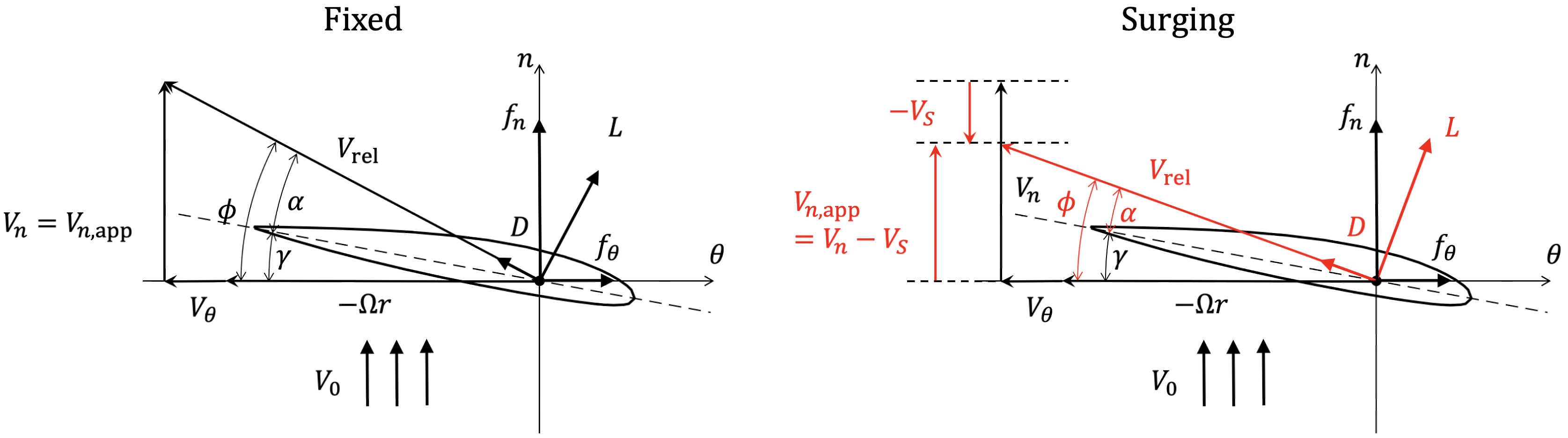
Figure 1: Velocity triangles of a blade element for fixed rotor (left) and surging rotor (right).

As for the parameter of ALM, each actuator line (blade) was represented with $40$ points with equidistant of $\Delta_{r}$, and the grid size $\Delta$ was designed to be similar as $\Delta_{r}$ for the wake region ($\Delta=D/80$, level 4 in Figure 2). Moreover, the smoothing factor $\varepsilon$ was set to $2\Delta$. The above settings were recommended by the proceeding studies Troldborg (2009); Sarlak et al. (2015); Martínez-Tossas et al. (2015). A tip correction factor $f_{\mathrm{tip}}$ with Glauert model was implemented to ensure the loads at the tip drop to zero Nathan et al. (2017), as shown in Equation 12. For modelling the hubs, additional actuator line elements with desired $C_{d}$ were introduced ($0.3$, and the reference area was the frontal area of hub) Cheeseman (1976); Naderi and Torabi (2017). Also, since that the concerned cord-based reduced frequencies (with respect to the considered surging frequencies) were relatively small, no dynamic-stall model was implemented for simplicity, and no aeroelastic codes were coupled.

The computational domains and meshes for the simulations are depicted in Figure 2, where Figure 2(b) was for the cases with laminar inflows ($10.4$M cells) and Figure 2(c) was for the cases with turbulent inflows ($10.9$M cells); the minor differences were mainly related to avoid undesired pressure fluctuations introduced by the synthetic turbulent inlet conditions. The meshes consists of cubic cells, and they were created through application snappyHexMesh. The Level in Figure 2 indicates the refinement levels, and the grid size $\Delta$ doubled as Level decreased by one (the two meshes shared the same value of $\Delta$ for the same Level). As described previously, $\Delta$ near the rotor (wake region) will be similar to the inter-distance of the actuator line points $\Delta_{r}$, meaning that $\Delta$ of Level 4 was $D/80$. Cartesian coordinate system was selected, with positive $x$ pointing to the downstream direction. The rotor center’s neutral position was located at the origin, and the rotor rotated in clockwise direction when being seen from the upstream. Regarding temporal resolution, there were $360$ time steps for the rotor to complete a revolution under its rated condition ($\Delta t=0.0138$ s). With this time step size $\Delta t$, the distance of the tip would travel $0.7\Delta$ in a time step, which was less than $1$ as recommended by previous works Troldborg (2009); Martínez-Tossas et al. (2015).

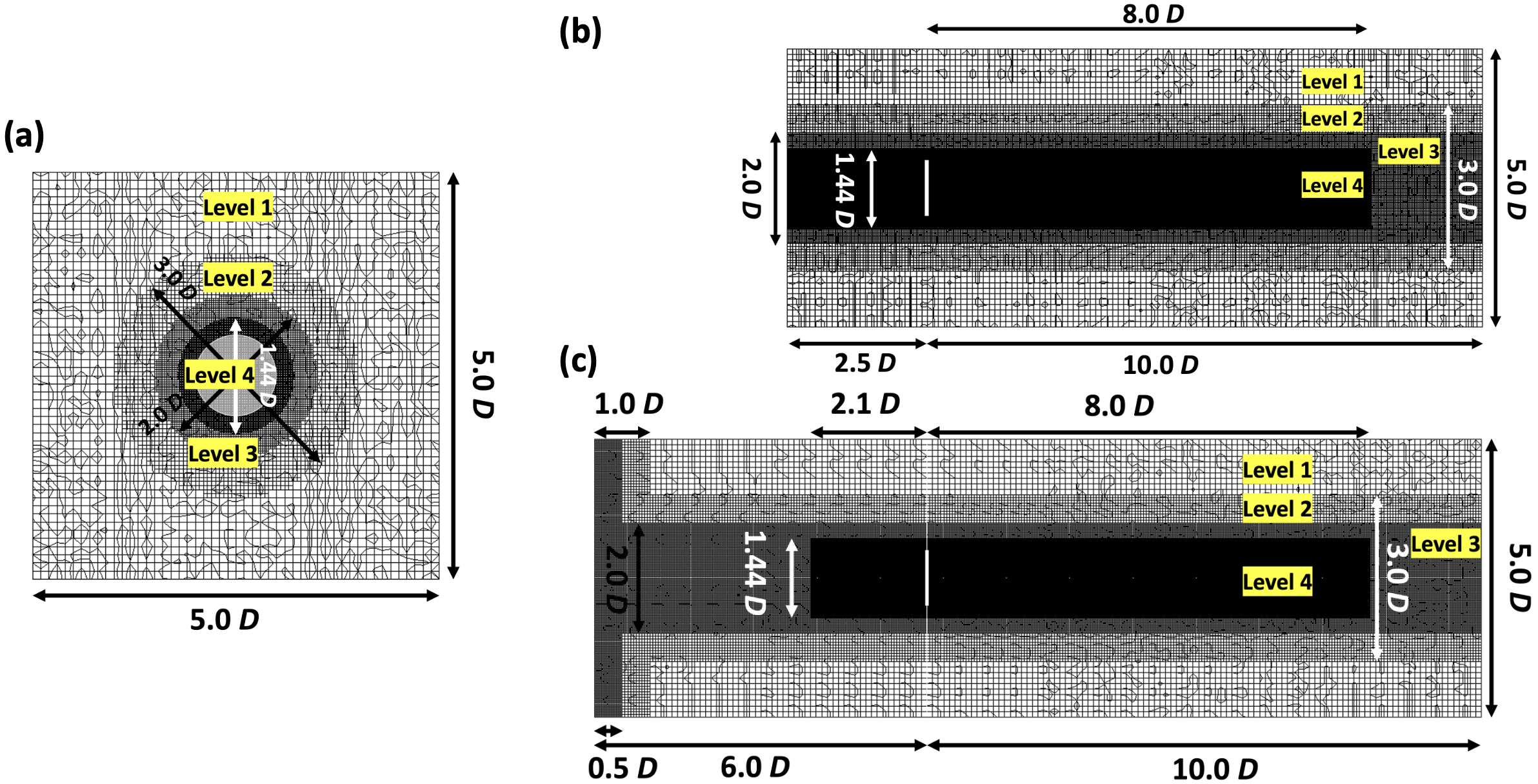
Figure 2: The mesh layouts for the simulation cases. (a) is the cross section of plane $x=0$ and it was shared by both laminar and turbulent cases. (b) and (c) are the cross sections of plane $y=0$, where (b) was for the laminar cases ($10.4$M cells) while (c) was for the turbulent ($10.9$M cells).

For the inlet boundary conditions, the laminar cases had velocity inlet with uniform fixed value, while the turbulent cases applied the divergence-free synthetic eddy method on their inlet, which is a built-in synthetic turbulent inlet conditions of OpenFOAM v2106 (turbulentDFSEMInlet). DFSEM are able to introduce inflow with desirable turbulence intensities, length scales, and anisotropy with much less computational efforts compare to the precursor method. Note that DFSEM are able to reproduce identical inflow in sense of both spatial and temporal, and this made the comparison of the instantaneous fields between cases meaningful. See Poletto et al. for more details about DFSEM Poletto et al. (2013). Other than the the inlet conditions of velocity, laminar cases and turbulent cases shared the same boundary conditions. The velocity boundary conditions of the four sides were treated as slip walls, and advective boundary condition ($\mathrm{D}/\mathrm{D}t=0$) was chosen for the outlet. As for the pressure fields, the four sides and the inlet were all assigned with symmetry boundary conditions, and the outlet was set to be an uniform fixed value, assuming the pressure fields had recovered to its ambient value at the outlet ($x/D=10$).

For more detail information about the simulation setups, please check the master’s thesis of Li Li (2023).

4 Verification and validation

4.1 Inflow turbulence characterization

The inflow turbulence were characterized $2.0D$ upstream from the rotor by several probes, as shown in Figure 3(a), they should not be characterized at the immediate inlet since the inflow turbulence would decay with the setups adopted. Several mean and turbulence properties were measured for different turbulent inflow conditions, including mean streamwise velocity $\overline{u}$, standard deviation of $u$ ($\sigma_{u}$ or $\overline{u^{\prime}u^{\prime}}$, similar with $v$ or $w$), turbulence intensity TI (Equation 13), power spectrum of $u$ ($S_{u}(f)$), and integral length scale of $u$ (in $x$-direction) $L_{u}$. Here the overline stands for the time-averaged (mean) operator and the prime stands for the fluctuation part, which is the well known Reynolds decomposition ($u=\overline{u}+u^{\prime}$). $L_{u}$ was defined as auto-correlation of $u$ first reached to zero. Note that $\overline{u}$, $\sigma_{u}$, $\sigma_{v}$, $\sigma_{w}$, and TI were obtained through averaging (equally weighted) all probes, while $L_{u}$ and $S_{u}(f)$ were obtained through the single probe located at the rotor center. Also notice that $V_{0}$ here was $11.4$ m/s.

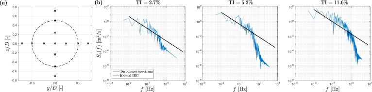
Figure 3: (a): Positions of the probes for sampling the inflow characteristics, they were located at $x/D=-2$. (b): Turbulence spectrum with different turbulent inflows.

$$\mathrm{TI}=\frac{\sqrt{\frac{1}{3}(\sigma_{u}^{2}+\sigma_{v}^{2}+\sigma_{w}^{2})}}{V_{0}}\times 100\%=\frac{\sqrt{\frac{2}{3}\mathrm{TKE}}}{V_{0}}\times 100\%$$ (13)

Table 1 listed out the quantities of the turbulent inflow conditions. Note that since the random seeds fed into DFSEM inlet conditions were same, the turbulent inflows generated by it were identical in space & time if other parameters remain the same, and this is an advantage for comparing cases. According to the international standard IEC 61400-1 edition 4.0 (2019) International Electrotechnical Commission (2019), $L_{u}$ should be $42$ m (Equation 14, $z$ is $90$ m for cases in this paper, which is the designed hub height) and $\sigma_{v}/\sigma_{u}$ should be bigger than $0.7$ (when floor is considered, $v$ is in lateral direction). Though $\sigma_{v}$ and $\sigma_{w}$ in Table 1 fulfilled IEC 61400-1, but $L_{u}$ seemed to be a bit larger. However, if consider some other standards in civil engineering realm (such as ASCE 7-16 & AIJ(2004)), $L_{u}$ in this case should be around $150$ to $250$ m Nandi and Yeo (2021). Thus, $L_{u}$ in Table 1 were considered to be realistic. Moreover, even though the three selected TI ($2.6$, $5.3$, & $11.6\%$) in Table 1 seemed to be lower than the values which IEC 61400-1 suggested (for class C with normal turbulence model, $\sigma_{u}/V_{0}$ should be $0.149$ as $V_{0}=11.4$ m/s), they were deemed valid since TI tends to be lower in offshore environments, while IEC standards were based on onshore conditions. Typically, TI for offshore conditions are around $5\%$ to $8\%$ Pollak (2014). Figure 3(b) shows the turbulence spectrum $S_{u}(f)$ measured by the probe at the center for different turbulent inflow conditions (parts with $f>V_{0}/2\Delta$ were truncated), the definition of the Kaimal spectrum adopted by IEC 61400-1 is in Equation 15 International Electrotechnical Commission (2019). Inertial ranges are clearly visible in Figure 3(b), and the spectrum also fitted Kaimal spectrum well.

Table 1: Turbulence characteristics measured at $2.0D$ upstream from rotor. Note that the length scales were measured only at the position of rotor center, and $V_{0}=11.4$ m/s.

TI [%]	$\overline{u}/V_{0}$	$L_{u}$ [m]	$\sigma_{u}/V_{0}$	$\sigma_{v}/\sigma_{u}$	$\sigma_{w}/\sigma_{u}$
2.66	$1.00$	$52.77$	$0.029$	$0.93$	$0.87$
5.32	$1.01$	$54.82$	$0.058$	$0.89$	$0.84$
11.62	$1.02$	$131.79$	$0.122$	$0.97$	$0.90$

$$L_{u}=0.7z,z\leq 60~{}\mathrm{m},\qquad L_{u}=42~{}\mathrm{m},z>60~{}\mathrm{m}$$ (14)

$$S_{u}(f)=0.05\sigma_{u}^{2}\left(\frac{L_{u}}{V_{0}}\right)^{-2/3}f^{-5/3}$$ (15)

4.2 Statistics

The averaging windows for the simulations were $20$ or $50T_{\Omega,\mathrm{rated}}$ (rotational period of rated condition) for the laminar or turbulent cases. With these windows, the interested statistics, including time-averaged & cycle-averaged rotor performances (eg. $\overline{C}_{T}$ & $<C_{T}>$), time-averaged & phase-locked averaged field values (eg. $\overline{u}$ & $<u>_{0\pi}$), and second order statistics (eg. $\sigma_{u}$ & $<\sigma_{u}>_{0\pi}$), were deemed converged. A brief results of convergence tests are presented in Appendix A. See Li Li (2023) for more detailed information about the sampling methods and the way to obtain statistics.

4.3 Grid related verification

Several aspects related to grid resolution were tested or checked. A simple grid independent test was performed in Appendix B, and it showed that the results were not sensitive to grid resolution. To check if LES simulations were conducted properly, the ratio of sub grid scale TKE ($k_{\mathrm{sgs}}$) over total TKE (resolved TKE + $k_{\mathrm{sgs}}$) were overviewed in Figure 4(a), showing that much more than $80\%$ of the TKE was resolved. Also, the undesired pressure fluctuations introduced by DFSEM were also checked with the fields of $\sigma_{p}$ (standard deviation of pressure fields) in Figure 4(b), showing that the pressure fluctuations were confined around the regions close to the inlet and had limited effects on the solutions after the rotor.

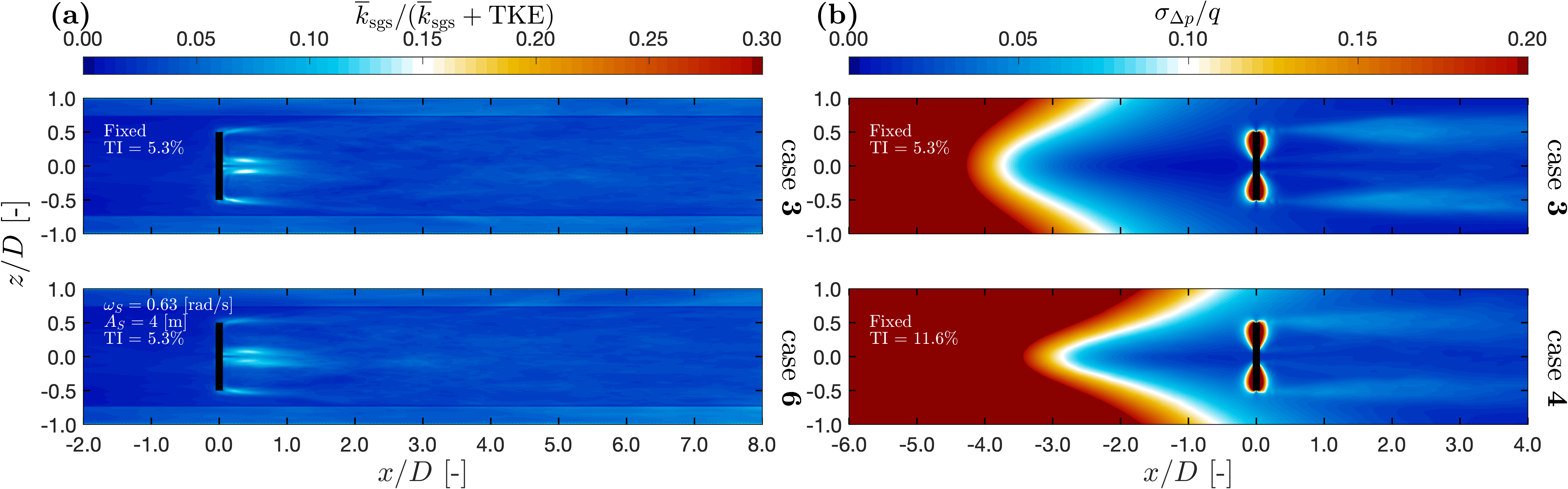
Figure 4: (a): Ratios of modeled turbulent kinetic energy ($\overline{k}_{\mathrm{sgs}}$) and total kinetic energy for case 3 (top) and case 11 (bottom). (b): The fields of pressure fluctuations for case 3 (top) and case 4 (bottom).

4.4 Validation

Table 2 displayed the values of $\overline{C}_{T}$ and $\overline{C}_{P}$ of the current work and other previous numerical studies of the fixed cases under rated conditions ($\lambda_{\mathrm{rated}}=7.00$, $V_{0,\mathrm{rated}}=11.4$ m/s). Even though the values of $\overline{C}_{T}$ and $\overline{C}_{P}$ from current works deviated quite away from the original design of Jonkman et al. Jonkman et al. (2009), they fell into the ranges as comparing to other works with various numeric methods, suggesting the values obtained were reasonable.

Table 2: Comparing $\overline{C}_{T}$ and $\overline{C}_{P}$ for fixed NREL 5MW rotor at its rated condition with other previous numeric works.

Source	Turbulence model	Force model	TI [$\%$]	$\overline{C}_{T}$	$\overline{C}_{P}$
Current work	LES	ALM	Laminar	$\mathbf{0.723}$	$\mathbf{0.510}$
Current work	LES	ALM	$\mathbf{5.3}$	$\mathbf{0.727}$	$\mathbf{0.519}$
Jonkman et al. Jonkman et al. (2009)	-	FAST	-	$0.81$	$0.47$
Johlas et al. Johlas et al. (2019)	LES	ALM	$4.1$	$0.752$	-
Xue et al. Xue et al. (2022)	LES	ALM	Laminar	$0.75$	$0.52$
Li et al. Li et al. (2015)	RANS	ALM	-	$0.77$	$0.49$
Yu et al. Yu et al. (2018)	RANS	ALM	-	$0.728$	$0.472$
Rezaeiha et al. Rezaeiha and Micallef (2021)	RANS	ADM	$5$	$0.715$	$0.567$

5 Results and Discussions

This section presents and discusses the simulation results. General wake characteristics and rotor performances for the considered cases can be found in Subsection 5.2, angle of attack for rotors with different surging settings can be found in Subsection 5.3, and selected field data are displayed in Section 5.4.

5.1 Test matrices

In total, there were 16 simulation cases, and there basic settings and results are in Table 3. Note that $<C_{T}>^{+}$ and $<C_{T}>^{-}$ minus represent the maximum and minimum values of $<C_{T}>$ for that case. To make visual comparison easier, values of $\overline{C}_{T}$ (time-averaged $C_{T}$) and $\overline{C}_{P}$ for the 16 cases were plotted with bar plot in Figure 5. $\overline{u}_{\mathrm{Disk}}^{3D}$ stands for the values of $\overline{u}_{\mathrm{Disk}}$ at $x/D=3$, similar rule for $\overline{u}_{\mathrm{Disk}}^{5D}$ and $\overline{u}_{\mathrm{Disk}}^{8D}$.

These 16 cases could be further categorized into two groups. The first group (Group 1) is the cases with a fixed or surging ($A_{S}=4$ m & $\omega_{S}=0.63$ rad/s) NREL 5MW rotor under different ambient turbulent intensities (TI), which are laminar, $2.7\%$, $5.3\%$, and $11.6\%$. They were grouped to investigate how the wake systems of fixed rotor differ from the surging rotor when under different inflow TI. There are eight cases in this group, with the four having a fixed rotor and the other having a surging rotor, corresponding to cases 1-4, 6 & 10-12. The second group (Group 2) consists the cases with six different surging settings under both laminar and turbulent inflow conditions (TI $=5.3\%$), where there are twelve cases (four of them were also in Group 1). The selected settings for $A_{S}$ & $\omega_{S}$ were $2$ m & $0.63$ rad/s, $4$ m & $0.63$ rad/s, $8$ m & $0.63$ rad/s, $4$ m & $0.32$ rad/s, $4$ m & $1.27$ rad/s, and fixed. Six of the cases were laminar (cases 1 & 5-9), and the other six were turbulent (cases 3, 11, & 13-16); note that inflow TI $=5.3\%$ is considered typical for offshore environments, whereas laminar inflow conditions are unrealistic.

Table 3: The basic settings and results for the cases conducted with single fixed or surging rotor of NREL 5MW baseline wind turbine at its rated condition ($V_{0}=11.4$ m/s, $\lambda=7$).

Case TI [$\%$] $A_{S}$ [m] $\omega_{S}$ [rad/s] $\mathbb{V}$ $\mathbb{W}$ $\overline{C}_{T}$ $<{C}_{T}>^{+}$ $<{C}_{T}>^{-}$ $\overline{C}_{P}$ $<{C}_{P}>^{+}$ $<{C}_{P}>^{-}$ $\overline{u}_{\mathrm{Disk}}^{3D}/V_{0}$ $\overline{u}_{\mathrm{Disk}}^{5D}/V_{0}$ $\overline{u}_{\mathrm{Disk}}^{8D}/V_{0}$ 1 Lam. Fixed Fixed $-$ $-$ $0.727$ $0.728$ $0.727$ $0.517$ $0.519$ $0.517$ $0.493$ $0.494$ $0.5165$ 2 $2.7$ Fixed Fixed $-$ $-$ $0.724$ $0.727$ $0.722$ $0.514$ $0.518$ $0.509$ $0.610$ $0.710$ $0.7922$ 3 $5.3$ Fixed Fixed $-$ $-$ $0.726$ $0.731$ $0.723$ $0.518$ $0.526$ $0.510$ $0.666$ $0.739$ $0.8114$ 4 $11.6$ Fixed Fixed $-$ $-$ $0.725$ $0.741$ $0.718$ $0.520$ $0.546$ $0.508$ $0.711$ $0.794$ $0.8487$ 5 Lam. $2$ $0.63$ $0.11$ $7.0$ $0.719$ $0.800$ $0.647$ $0.519$ $0.643$ $0.394$ $0.517$ $0.556$ $0.7143$ 6 Lam. $4$ $0.63$ $0.22$ $7.0$ $0.715$ $0.855$ $0.542$ $0.523$ $0.776$ $0.272$ $0.535$ $0.587$ $0.6956$ 7 Lam. $8$ $0.63$ $0.44$ $7.0$ $0.673$ $0.873$ $0.346$ $0.516$ $0.857$ $0.097$ $0.582$ $0.609$ $0.7238$ 8 Lam. $4$ $0.32$ $0.11$ $3.5$ $0.724$ $0.800$ $0.642$ $0.518$ $0.648$ $0.392$ $0.510$ $0.540$ $0.6942$ 9 Lam. $4$ $1.27$ $0.44$ $14.0$ $0.671$ $0.871$ $0.339$ $0.515$ $0.856$ $0.094$ $0.575$ $0.604$ $0.7260$ 10 $2.7$ $4$ $0.63$ $0.22$ $7.0$ $0.714$ $0.853$ $0.539$ $0.522$ $0.772$ $0.269$ $0.615$ $0.720$ $0.8106$ 11 $5.3$ $4$ $0.63$ $0.22$ $7.0$ $0.716$ $0.853$ $0.541$ $0.526$ $0.773$ $0.274$ $0.664$ $0.760$ $0.8179$ 12 $11.6$ $4$ $0.63$ $0.22$ $7.0$ $0.713$ $0.845$ $0.543$ $0.525$ $0.761$ $0.276$ $0.719$ $0.799$ $0.8541$ 13 $5.3$ $2$ $0.63$ $0.11$ $7.0$ $0.725$ $0.799$ $0.640$ $0.522$ $0.651$ $0.392$ $0.664$ $0.746$ $0.8109$ 14 $5.3$ $8$ $0.63$ $0.44$ $7.0$ $0.673$ $0.867$ $0.345$ $0.516$ $0.853$ $0.098$ $0.686$ $0.764$ $0.8260$ 15 $5.3$ $4$ $0.32$ $0.11$ $3.5$ $0.725$ $0.800$ $0.641$ $0.522$ $0.656$ $0.393$ $0.667$ $0.748$ $0.8093$ 16 $5.3$ $4$ $1.27$ $0.44$ $14.0$ $0.672$ $0.864$ $0.342$ $0.516$ $0.850$ $0.099$ $0.698$ $0.766$ $0.8295$

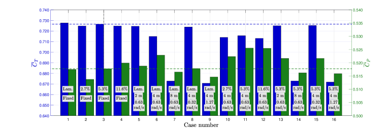
Figure 5: Bar plots of $\overline{C}_{T}$ and $\overline{C}_{P}$ for the 16 cases. Entries on each bar are for inflow TI (top), $A_{S}$ (middle), and $\omega_{S}$ (bottom). Values of fixed turbulent case (case 3, TI$=5.3\%$) was chosen to be the reference values for comparison.

5.2 Summarizing wake characteristics and rotor performances

5.2.1 Cases of fixed and surging rotor with different inflow TI

Figure 6 plots out the profiles of time-averaged streamwise velocity $\overline{u}$ for the eight cases of Group 1. First, by focusing on the two cases with laminar inflow conditions (one had fixed rotor and the other had surging), it was found that $\overline{u}$ profiles for the two cases were very similar when $x/D=3$ but significantly differed at $x/D=8$, pointing out the case with fixed rotor had different dynamics of wake system compare to the case with surging rotor when the inflow was laminar. Moreover, $\overline{u}$ profiles of the fixed case retained very similar from $x/D=3$ to $8$, suggesting that mixing and recoveries were weak; while for the surging case, the profile of $\overline{u}$ changed and the values of $\overline{u}$ increased as they traveled downstream, suggesting that recoveries occurred. Next, considering the other six turbulent cases, it can be found that the profiles of $\overline{u}$ between the fixed and surging cases with same inflow TI were quite similar all the way form $x/D=3$ to $8$, showing the wake systems of turbulent cases were not as sensitive to whether the rotor was surging as the laminar cases. Furthermore, it was shown that $\overline{u}$ (within the projection zone of the rotor, $\lvert{z/D}\rvert\leq 0.5$) recovered faster with stronger ambient turbulence for both surging and fixed cases, and all the six turbulent cases recovered faster than the laminar cases. Additionally, their $\overline{u}$ profiles all eventually appeared in Gaussian-shape.

Figure 7(a) plots the profiles of mean disk-averaged streamwise velocity $\overline{u}_{\mathrm{Disk}}$ along the $x$ direction for the eight cases of Group 1. The effects of surging on wake recovery rates with different TI can be estimated with profiles of $\overline{u}_{\mathrm{Disk}}$. The two laminar cases had very different $\overline{u}_{\mathrm{Disk}}$ profiles, where the surging case displayed significant recoveries on $\overline{u}_{\mathrm{Disk}}$ after the rotor ($x/D=0$) but the fixed case did not. As for the turbulent cases, the profiles of $\overline{u}_{\mathrm{Disk}}$ were similar between the fixed and surging cases, as long as the input TI was the same. However, if looking closely, it can be found that the surging cases tend to have slightly larger $\overline{u}_{\mathrm{Disk}}$ compared to the fixed cases. The relative differences of $\overline{u}_{\mathrm{Disk}}$ at $x/D=3$, $5$, and $8$ can be found in Table 4. The values in the table show that the differences of $\overline{u}_{\mathrm{Disk}}$ between the fixed and surging cases for laminar cases were pronounced, where $\overline{u}_{\mathrm{Disk}}$ for surging case at $x/D=5$ & $8$ were $18.8\%$ & $34.7\%$ larger than the fixed cases; while for the turbulent cases, $\overline{u}_{\mathrm{Disk}}$ became much more similar between the fixed and surging cases, with merely about $0.5\sim 2\%$ gains of $\overline{u}_{\mathrm{Disk}}$ at $x/D=5$ & $8$ for the three inflow TI considered. Although the gains in $\overline{u}_{\mathrm{Disk}}$ due to the surging were quite mild for the turbulent cases, it should be noted that the surging cases already had higher values for $\overline{C}_{P}$, and both larger $\overline{u}_{\mathrm{Disk}}$ and higher $\overline{C}_{P}$ have beneficial effects on overall power outputs at the wind farm level.

Another interesting thing with $\overline{u}_{\mathrm{Disk}}$ if looking closely in Figure 7(a) is that the profiles of $\overline{u}_{\mathrm{Disk}}$ (induction fields) just before the rotor ($x/D\simeq 0$) were more dominated by whether the rotor was surging or fixed. While after the rotor, the profiles of $\overline{u}_{\mathrm{Disk}}$ were more influenced by inflow TI.

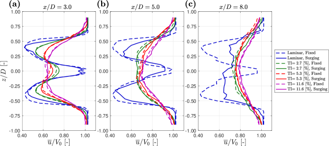
Figure 6: Profiles of $\overline{u}$ at different $x/D$ for cases of fixed or surging rotor with different inflow TI. (a) $x/D=3$, (b) $x/D=5$, (c) $x/D=8$

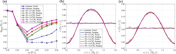
Figure 7: (a) $\overline{u}_{\mathrm{Disk}}$ along $x$-direction for cases of fixed or surging rotor with different inflow TI. (b)-(c) $<C_{T}>$ and $<C_{P}>$ for cases of fixed or surging rotor with different inflow TI.

Table 4: The ratios of $\overline{u}_{\mathrm{Disk}}$ for the fixed and surging cases under different inflow TI at $x/D=3$, $5$, and $8$.

Laminar TI $=2.7\%$ TI $=5.3\%$ TI $=11.6\%$ $\overline{u}_{\mathrm{Disk,surging}}^{3D}/\overline{u}_{\mathrm{Disk,fixed}}^{3D}$ $108.52\%$ $100.82\%$ $99.70\%$ $101.13\%$ $\overline{u}_{\mathrm{Disk,surging}}^{5D}/\overline{u}_{\mathrm{Disk,fixed}}^{5D}$ $118.83\%$ $101.41\%$ $102.84\%$ $100.63\%$ $\overline{u}_{\mathrm{Disk,surging}}^{8D}/\overline{u}_{\mathrm{Disk,fixed}}^{8D}$ $134.70\%$ $102.31\%$ $100.80\%$ $100.64\%$

Figure 7(b) & 7(c) display cycle-averaged $C_{T}$ & $C_{P}$ ($<C_{T}>$ & $<C_{P}>$) for the eight cases of Group 1. Note that for fixed cases, the reference period for cycle average was set to $2T_{\Omega}$, which was the same as $T_{S}$ for the surging cases considered here. It is obvious that the curves of $<C_{T}>$ & $<C_{P}>$ were insensitive to the inflow TI, and the fixed cases had almost constant values while the surging cases had values that varied periodically according to $\phi_{S}$ with respect to the surging motions. Note that since the displacements of the rotor for the four cases were written as $A_{S}\sin\omega_{S}<t>$, the surging velocity of the rotor $V_{S}$ would be $\omega_{S}A_{S}\cos\omega_{S}<t>$ (Equations 1 & 2). Thus at $<t=0>$, the rotor was moving along with the free-stream ($V_{0}$), making the apparent inflow velocity perceived by the rotor $V_{0,\mathrm{app}}$ smaller, and this resulted in relatively smaller values for $<C_{T}>$ and $<C_{P}>$ at $<t>=0$.

5.2.2 Cases with different surging settings under laminar or turbulent inflow conditions

Figure 8 plotted out $\overline{u}_{\mathrm{Disk}}$ for the twelve cases of Group 2. Profiles of $\overline{u}$ were not presented since they shared similar features with the previous cases, where laminar cases had profiles with kinks and turbulent cases had Gaussian-shape profiles.

For the laminar cases, it is obvious that surging did facilitate recoveries of $\overline{u}_{\mathrm{Disk}}$ (Figure 8(a)), and cases with bigger $A_{S}$ & $\omega_{S}$ ($\mathbb{V}$) had higher $\overline{u}_{\mathrm{Disk}}$ up until $x/D=6$. In general, it showed that the trends for $\overline{u}_{\mathrm{Disk}}$ profiles were related to $\mathbb{V}$ (see Table 3), and higher $\mathbb{V}$ would result in larger values for $\overline{u}_{\mathrm{Disk}}$. However, interestingly, for $x/D\geq 7$, the values of $\overline{u}_{\mathrm{Disk}}$ seemed to converge to a similar value. Chen et al. Chen et al. (2022) had reported a similar trend.

For the turbulent cases, unlike the cases with laminar inflow conditions presented previously, the differences of $\overline{u}_{\mathrm{Disk}}$ between fixed cases and surging cases were not very pronounced (Figure 8(b)). However, it can be seen that $\overline{u}_{\mathrm{Disk}}$ for surging cases were slightly larger compared to the fixed case, and $\overline{u}_{\mathrm{Disk}}$ appeared to have larger values with bigger $A_{S}$ and $\omega_{S}$, suggesting that larger $\mathbb{V}$ may have positive effects on wake recovery under the conditions of realistic turbulent inflows; additionally, it should be noted that cases with some surging settings had smaller values for $\overline{C}_{T}$ (eg. cases with $\mathbb{V}=0.44$), which suggested milder blockage effects, and milder blockage would also contribute to larger $\overline{u}_{\mathrm{Disk}}$, while the effects were not quantified in this paper.

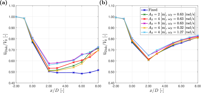
Figure 8: $\overline{u}_{\mathrm{Disk}}$ along $x$-direction for cases of rotor with different surging settings under laminar or turbulent inflow conditions. (a) Laminar (b) Turbulent (TI $=5.3\%$).

Figures 9(a) and 9(b) display $<C_{T}>$ for the twelve cases of Group 2, and the values of $\overline{C}_{T}$ and $\overline{C}_{P}$ can be found in Table 3. Here, we can clearly see that $<C_{T}>$ for the surging cases varied periodically according to $\omega_{S}$ of their case, and larger $\mathbb{V}$ brought larger varying amplitudes. Moreover, it was found that $<C_{T}>$ were essentially the same between the laminar cases and the turbulent cases for all the six considered surging settings, again showing that cycle-averaged rotor performances were insensitive to inflow turbulence. Furthermore, it seemed that there was an upper limit for $<C_{T}>$, and the $<C_{T}>$ curves of cases with higher $\mathbb{V}$ ($\mathbb{V}=0.44$) dropped after reaching the limit. This limit was related to stalling, which will be further elaborated in Section 5.3. Moreover, by looking at the values of $<C_{T}>^{+}$ and $<C_{T}>^{-}$ (maximum and minimum of $<C_{T}>$) for the surging cases in Table 3, it can be seen that $<C_{T}>^{-}$ were further away from $\overline{C}_{T}$ of the fixed cases compared to $<C_{T}>^{+}$, and this was reflected in smaller $\overline{C}_{T}$ for the surging cases than the fixed cases, especially for the cases with bigger $\mathbb{V}$. However, focusing on the values of $\overline{C}_{P}$, it appeared that the surging cases with smaller $\mathbb{V}$ ($\mathbb{V}=0.11$ or $0.22$) had slightly bigger values compared to the fixed case, while the opposite happened for the cases with bigger $\mathbb{V}$ ($\mathbb{V}=0.44$). It was suggested that the velocity triangle and stalling can be used to explain these behaviors of $\overline{C}_{T}$ & $\overline{C}_{P}$. More detailed discussions on stalling and the causes of lower $\overline{C}_{T}$ for surging rotor can be found in Section 6.

Further observing the curves of $<C_{T}>$ in Figures 9(a) & 9(b), one can find that they were almost in-phase with the surging motions, and this agreed with most of the findings in the literature Tran and Kim (2016); Arabgolarcheh et al. (2022); Ferreira et al. (2022). It can be seen that the curves of $<C_{T}>$ and $<C_{P}>$ crossed the values of the fixed case around $<t>/T_{\Omega}=0.5$ and $1.5$, which were the timing when the rotor had zero surging velocity ($\phi_{S}=0.5\pi$ or $1.5\pi$, $V_{S}=0$ m/s). However, slight hysteresis effects still appeared after plotting $<C_{T}>$ against the surging velocity of the rotor $V_{S}$ in Figure 9(c). Notice that $V_{S}$ reflected the phase of surging (Equation 2). The hollow marks in Figure 9(c) represent the minimums and maximums of $<C_{T}>$ a case should obtain according to quasi-steady solutions of the auxiliary simulation cases in Table 5. Notably in Figure 9(c), cases with $A_{S}=8$ m & $\omega_{S}=0.63$ rad/s and $A_{S}=4$ m & $\omega_{S}=1.27$ rad/s (cases with $\mathbb{V}=0.44$) had more significant hysteresis effects, and they were also more pronounced for cases with higher $\omega_{S}$. That is, the extent of the hysteresis effects depended on both $\mathbb{V}$ and $\mathbb{W}$ ($\omega_{S}$), and larger values of $\mathbb{V}$ or $\mathbb{W}$ would result in stronger hysteresis effects. Moreover, for all the surging cases, hysteresis effects were more pronounced as the rotor moved along the free stream direction, where the rotor surged into its wake.

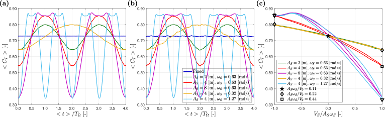
Figure 9: $<C_{T}>$ for cases with different surging settings, where (a) presents cases under laminar inflows and (b) presents cases under turbulent inflows. (c): $<C_{T}>$ against $V_{S}$. Where the hollow marks were the values predicted with quasi-steady simulation cases listed in Table 5.

5.3 Angle of attack and stalling

This subsection examines the stalling phenomena of surging wind turbine rotor with different surging settings by analyzing the angle of attack $\alpha$. As $V_{0,\mathrm{app}}$ became large enough to make the angle of attack $\alpha$ of a blade section exceed the stalling angle $\alpha_{\mathrm{stall}}$ through the enlarged inflow angle $\phi$ (Equation 10), that blade section would experience stalling and made its $C_{l}$ drop while $C_{d}$ rise, causing both $C_{T}$ and $C_{P}$ to drop. Note that since ALM was implemented, stalling behaviors were modeled through the input polar data; only the values of $C_{l}$ and $C_{d}$ were concerned, and no additional effects such as extra turbulence from the boundary layer development nor leading edge vortex generated due to stalling were modeled. Also, one should note that the polar data used in this study were static polar and no dynamic-stall model was applied.

Figure 10 presents the cycle-averaged $\alpha$ ($<\alpha>$) along the blade during a surging cycle based on $\phi_{S}$ for the surging cases with different surging settings, and $<\alpha>$ for the fixed case are also presented (based on $<t>$) for comparison (cases 1, 5, & 6-9); note that the cases presented in Figure 10 were all under laminar inflow conditions. Here $\alpha_{\mathrm{stall}}$ is stalling angle of attack, and $\alpha_{\mathrm{stall}}$ was defined at $\alpha$ which gave the (first local) maximum $C_{l}$. Profiles of $\alpha_{\mathrm{stall}}$ for NREL 5MW baseline turbine along its blade span can be found in Appendix D. Note that the airfoil geometries were not fixed along the blade span, causing the profiles of $<\alpha>/\alpha_{\mathrm{stall}}$ in Figure 10 had some abrupt changes. It is clear that $<\alpha>$ for the fixed case in Figure 10 can be considered as constants, and stalling phenomena did not occur. While for the surging cases, the patterns of $<\alpha>$ for cases with the same $\mathbb{V}$ were almost identical, and the stalling effects were more prominent with higher $\mathbb{V}$. Together with Equation 2, Figure 10 demonstrates stalling occur most significantly when the rotor was moving against the inflow, as $V_{0,\mathrm{app}}$ & $V_{n,\mathrm{app}}$ had bigger values. Note that stalling mostly occurred at the sections closer to the root, and this was as expected since $\alpha$ close to the root was more subjected to variations of $V_{n,\mathrm{app}}$ due to the fact that $\Omega r$ was smaller (Equation 10). Moreover, since the timings of stalling were aligned with the dips of $<C_{T}>$ for the surging cases with $\mathbb{V}=0.44$ as $\phi_{S}=\pi$ (Figure 9(a)), it can be concluded that stalling was the cause of the dips on the curves.

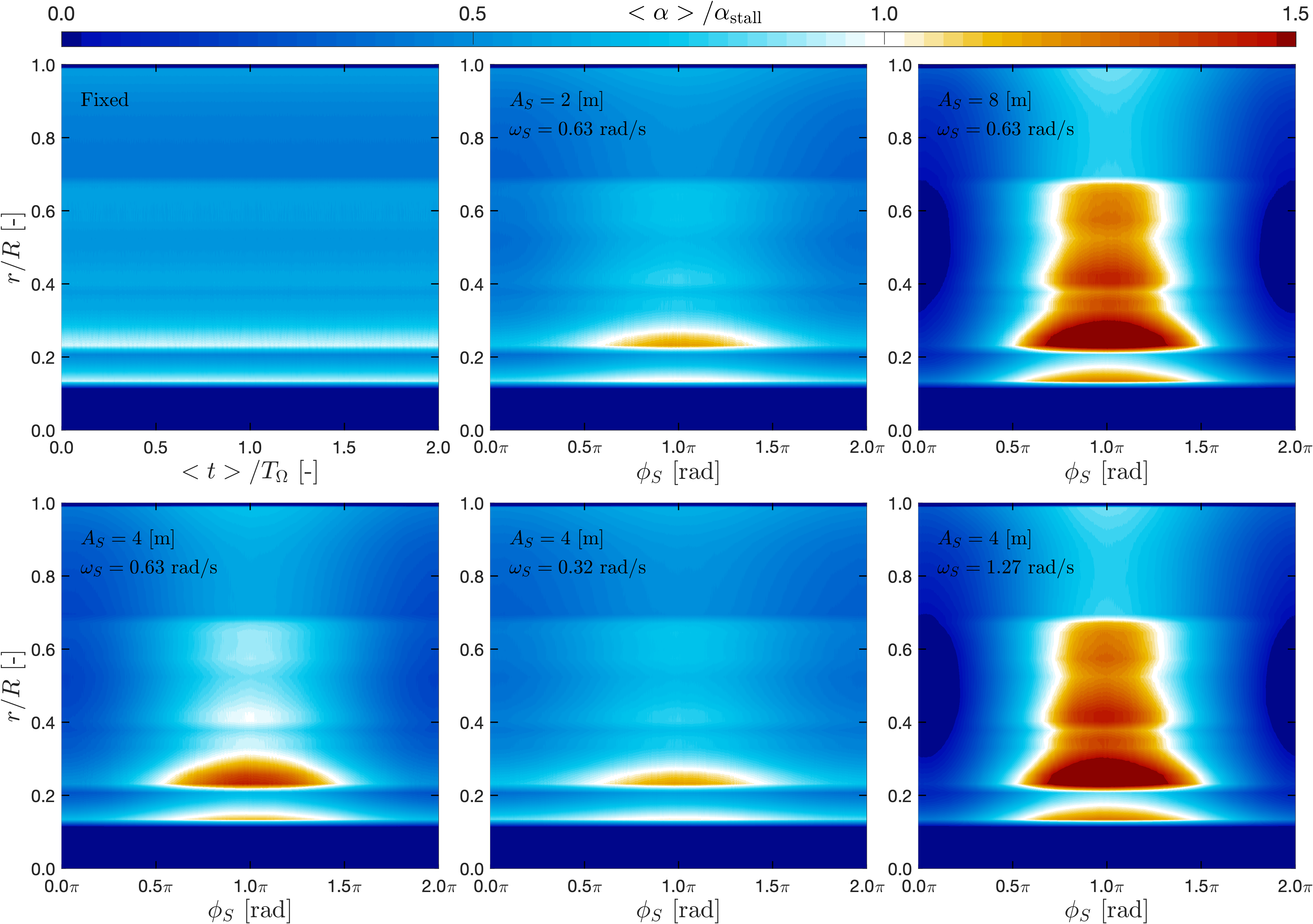
Figure 10: Cycle-averaged angle of attack $<\alpha>$ for cases with different surging settings under laminar inflow conditions. Note that for the fixed case (top left), the reference of cycle-averaging for $<\alpha>$ was based on $<t>$ instead of $\phi_{S}$.

5.4 Fields data

This subsection presents and discusses the contours of the selected field data. The selected fields were instantaneous streamwise velocity ($u$), phase-locked averaged streamwise velocity ($<u>_{0\pi}$), phase-locked turbulent kinetic energy ($<$TKE$>_{0\pi}$), turbulent kinetic energy (TKE), phase-locked averaged $y$-component vorticity fields ($<\omega_{y}>_{0\pi}$), and terms related to momentum entrainment. Note that not all the cases for each of the fields were presented. See Li Li (2023) for more comprehensive results.

5.4.1 Instantaneous streamwise velocity fields

The instantaneous contours of streamwise velocity $u$ for cases of Group 1 are displayed in Figure 11. It is clear that cases with higher TI had more prominent fluctuations with $u$. For the two laminar cases, the wake structures of the fixed case were relatively stable, and the breakdown process began at around $x/D=6.5$ to $8.0$; while some periodic structures (Surging Induced Periodic Coherent Structures, (SIPCS)) were clearly visible in the wake of the surging case, and they started to decay at around $x/D=5$. As for the six turbulent cases, although surging motions altered the wake system significantly for the laminar cases, the instantaneous wake systems for the turbulent cases with fixed rotor were quite similar with the surging cases as comparing their $u$ fields in Figure 11 (at least for $x/D\leq 4$), especially for cases with higher TI; this comparison was deemed valid since the generated inflows with same inflow TI were considered identical with the synthetic turbulent inlet. The mentioned resemblance for the wake structures between the fixed and surging cases under turbulent inflows indicated that instantaneous wake structures were primarily influenced by the inflow turbulence, rather than whether or not the rotor was surging.

The contours of $u$ fields for the twelve cases of Group 2 were not presented since they had similar features that had already been discussed. That is, SIPCS could be detected for the laminar cases, and the instantaneous wake structures were more dominated by inflow turbulence for the turbulent cases. SIPCS were hardly identified and surging settings had little effects on the fields of $u$.

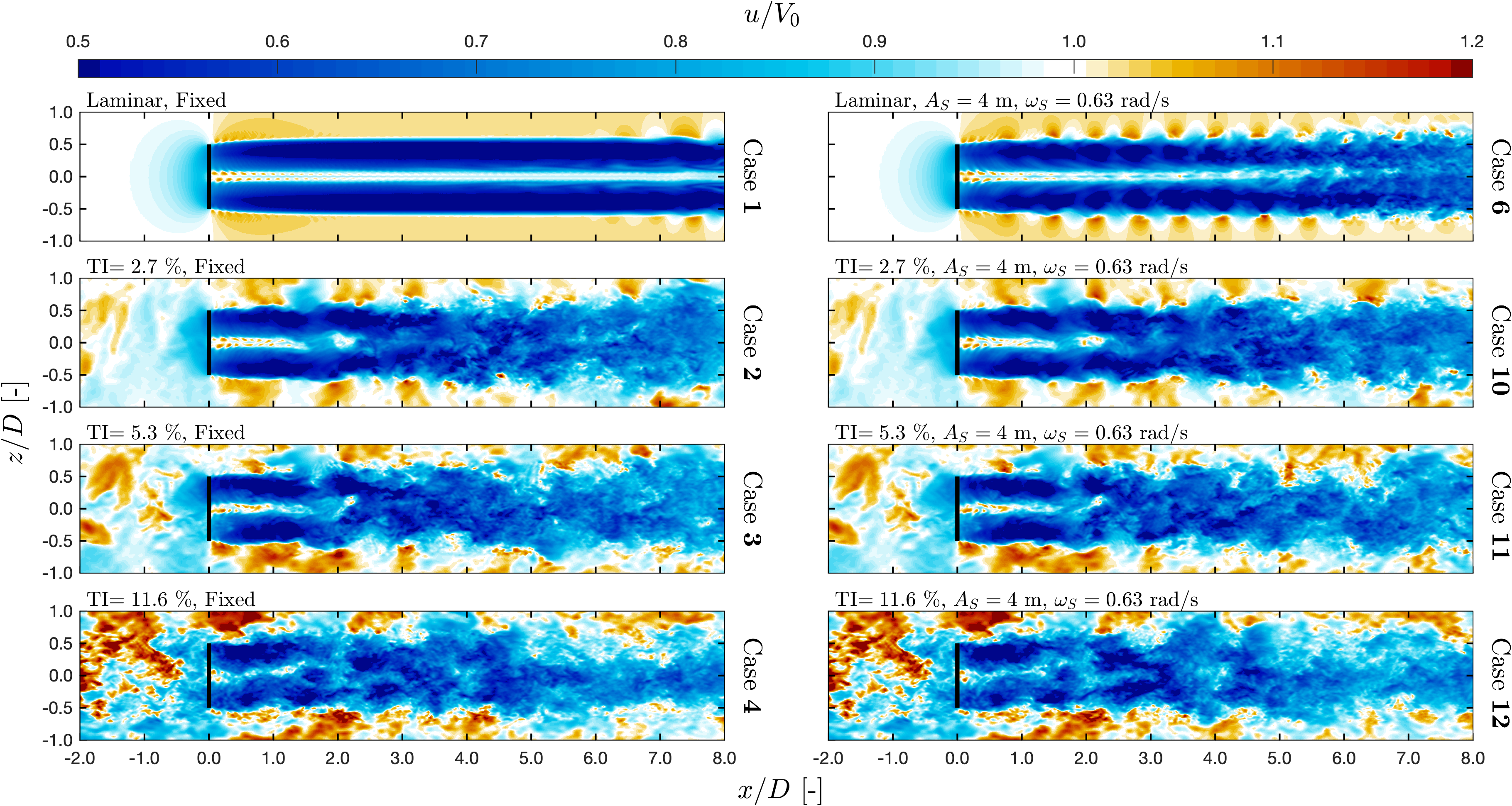
Figure 11: Fields of instantaneous streamwise velocity fields $u$. The left four cases had fixed rotor while the right four had surging. Inflow conditions for each rows were identical.

5.4.2 Phase-locked averaged streamwise velocity fields

The phase-locked averaged streamwise velocity fields as $\phi_{S}=0\pi$ (or $\phi_{\Omega}=0\pi$) $<u>_{0\pi}$ of the four selected cases (cases 1, 3, 6, & 11) are displayed in Figure 12. The way of phase-locked averaging was described in Section 2. One should note that the phase-locked properties were both applicable for $\phi_{\Omega}$ and $\phi_{S}$ since they were synchronized. Also that the four selected cases represent the fixed/surging cases under laminar/turbulent inflow conditions, which they were able to depict the general features of the 16 cases. Comparing $<u>_{0\pi}$ fields in Figure 12 with the $u$ fields in Figure 11, the effects of tip and root vorticies for the turbulent cases (cases 3 & 11) became more observable and more similar to the laminar ones for both fixed and surging cases. Moreover, for the surging cases, they also displayed similar periodic structures as laminar cases. Pairs of surging related periodic coherent structures were observed. We called them Surging Induced Periodic Coherent Structures (SIPCS), which features lower $u$ at the inner region of the wake and higher $u$ at the outer (boxes of red dashed-line in Figure 12); Kleine et al. Kleine et al. (2022) had also reported these structures. More details about SIPCS will be displayed and discussed with $<\omega_{y}>_{0\pi}$ fields later and in Section 7.

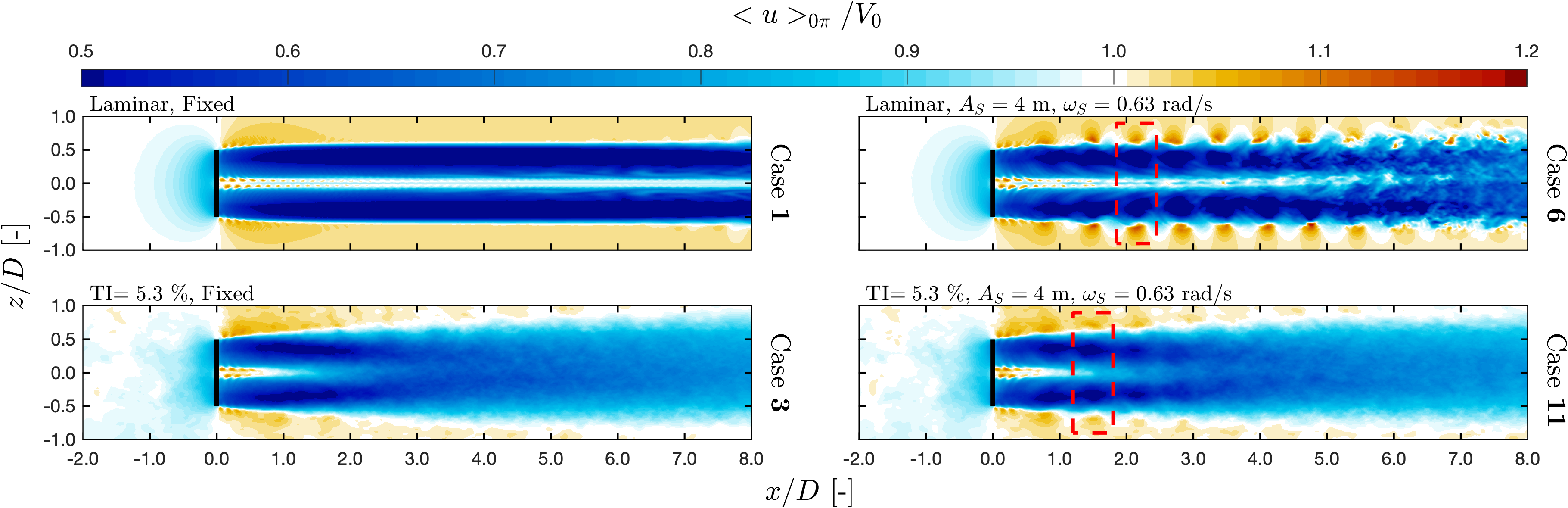
Figure 12: Fields of phase-locked averaged streamwise velocity fields $<u>_{0\pi}$. SIPCS for the surigng cases were enclosed by boxed of red dashed-line boxes. Top left: Fixed laminar. Bottom left: Fixed turbulent. Top right: surging laminar. Bottom right: Surging turbulent.

5.4.3 Phase-locked turbulent kinetic energy fields

The phase-locked turbulent kinetic energy $<$TKE$>_{0\pi}$ fields of the eight selected cases (cases 1, 3, 5-9, & 11) are shown in Figure 13. The definition of $<$TKE$>_{0\pi}$ is in Section 2, and the main purpose of introducing it is to measure the extent of the repeatability of the flow fields with the certain periods (for surging cases were $T_{S}$, while for fixed cases were $2T_{\Omega}$). The eight selected cases covered cases with different surging settings under laminar inflow conditions and two cases under turbulent inflow conditions with fixed or surging rotor. Regarding the very low $<$TKE$>_{0\pi}$ fields for the six laminar cases with different surging settings (even at the vicinity of the rotor), it was shown that the flow fields for laminar cases were highly periodic and repeatable with respect to surging period $T_{S}$; it was quite surprising that values of $<$TKE$>_{0\pi}$ were very low globally even with the presence of complex flow structures introduced by the surging rotor. Moreover, the very low values for $<$TKE$>_{0\pi}$ fields also reflected on the $\overline{u}$ profiles in Figure 6, where the laminar surging case (case 6) had profiles of $\overline{u}$ with kinks. The kinks were due to the highly localized flow structures (SIPCS) always passing through the specific positions repeatedly, making the statistics at some regions differ from those in their vicinity. Furthermore, if comparing $u$ fields and $<u>_{0\pi}$ fields of the six laminar cases in Figures 11 & 12 closely, one can find they were almost identical, which supported the very low values of $<$TKE$>_{0\pi}$ fields. Also, an interesting phenomenon was that with bigger $A_{S}$, the values of $<$TKE$>_{0\pi}$ fields seemed to be smaller (eg. compare cases 1 & 5-7 in Figure 13), and the fixed case had the biggest values. Fang et al. Fang et al. (2021) had reported similar phenomena using IDDES with geometric resolved rotor, stating that tip-vorticity related structures actually broke-up earlier while the rotor was fixed compared to a surging one. The above phenomenon implied that with bigger $A_{S}$, the flow fields actually became more repeatable. As for $\omega_{S}$, the trend with respect to it was not obvious, but it was still clear that the surging cases had lower values for $<$TKE$>_{0\pi}$ fields when comparing to the fixed case under laminar inflow. As for the turbulent cases, effects of tip and root vorticies were revealed with $<$TKE$>_{0\pi}$ fields, and periodic structures related to SIPCS could be once more observed for the case with surging rotor, where case with fixed rotor did not have (cases with other surging settings had similar features).

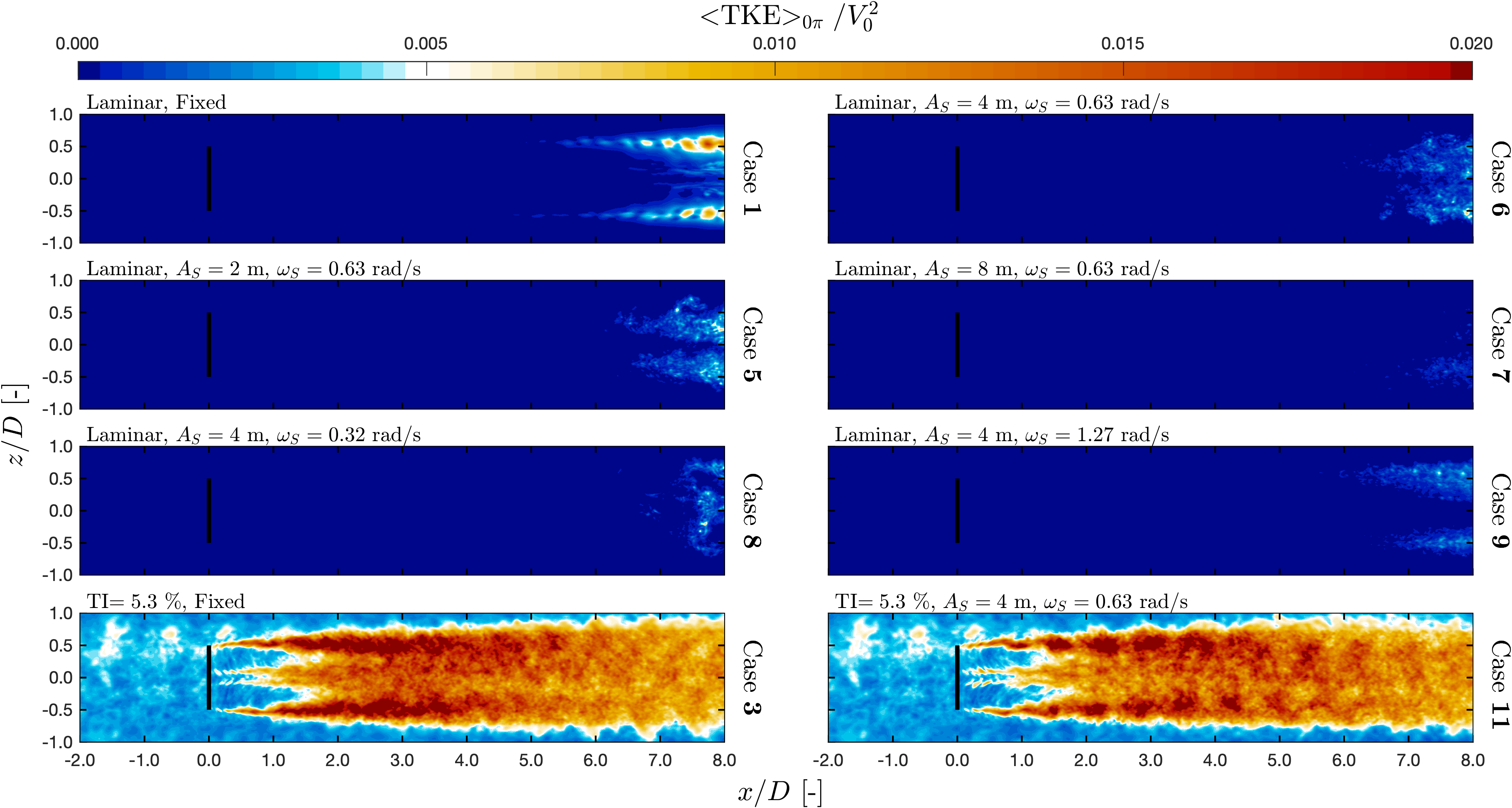
Figure 13: Fields of phase-locked averaged turbulent kinetic energy $<$TKE$>_{0\pi}$. Top three rows: Cases with different surging settings under laminar inflow conditions. Bottom row: A fixed case and a surging case under turbulent inflow conditions.

5.4.4 Turbulent kinetic energy fields

The fields of turbulent kinetic energy TKE of the four selected cases (cases 1, 3, 6, & 11) are shown in Figure 14. Again, these four selected cases were capable of representing the general features of TKE fields for fixed/surging rotor under laminar/turbulent inflow conditions. Unlike $<$TKE$>_{0\pi}$ only considered certain time steps with relative large intervals, TKE considered all of the available time steps, and thus it can serve as an indicator for general flow fluctuations. For the turbulent case with fixed rotor (case 3), the patterns of TKE and $<$TKE$>_{0\pi}$ were alike, except for the regions just behind the rotor, where the geometric information of the rotor was still remembered by the wake. As for the laminar case with fixed rotor (case 1), regarding the very low values for TKE field (except at the region vicinity to the rotor), the flow was not just highly repeatable, it was essentially without fluctuations. While for the TKE field of the turbulent case with surging rotor (case 11), they were very similar to the cases with fixed rotor when under the same inflow TI. As for the laminar case with surging rotor (case 6), there were two strips of regions having higher TKE after the tip of the rotor; they were related to the convection of SIPCS which will be discussed later.

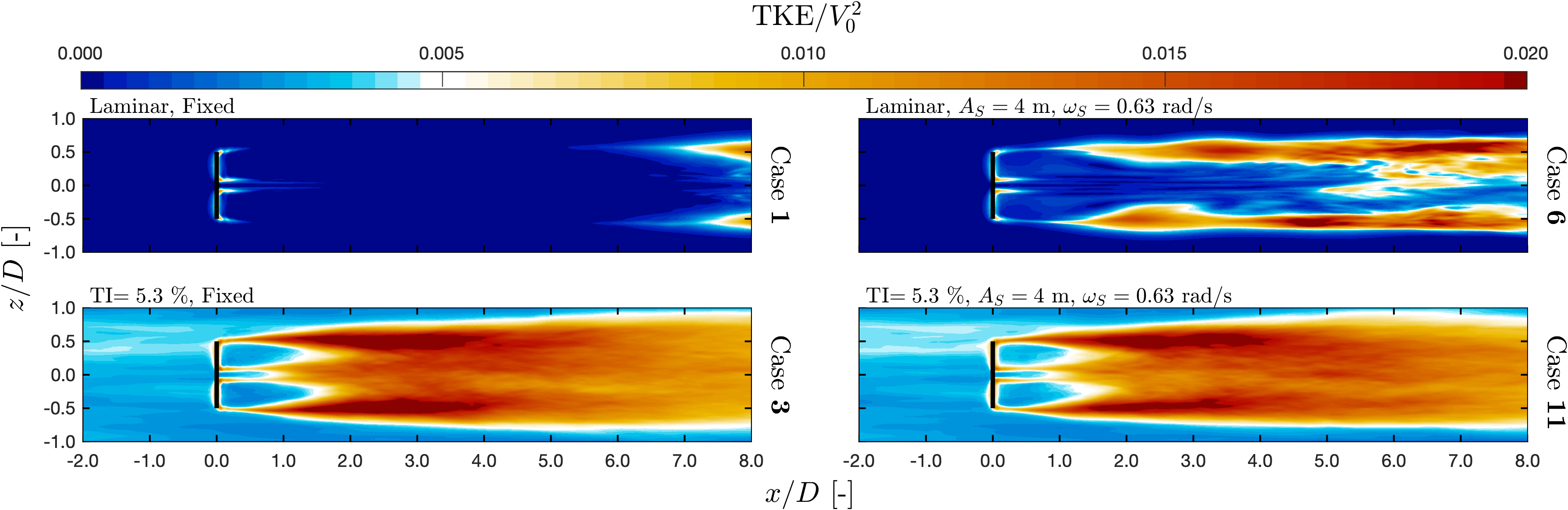
Figure 14: Fields of turbulent kinetic energy TKE. Top left: Fixed laminar. Bottom left: Fixed turbulent. Top right: surging laminar. Bottom right: Surging turbulent.

5.4.5 Phase-locked averaged $y$-component (out-of-plane) vorticity fields

The phase-locked averaged $y$-component (out-of-plane) vorticity fields $<\omega_{y}>_{0\pi}$ are presented in Figure 15. For this case, all 16 cases in Table 3 are presented, and more detail comparisons between cases are carried out, especially about the SIPCS.

The distributions of $<\omega_{y}>_{0\pi}$ for the four fixed cases (cases 1-4) were as expected, regions with higher magnitudes were mainly concentrating at the regions behind the tips and roots, accounting for the released trailing (tip and root) vorticies, and they remained quite obvious til $x/D=2$ even with the highest considered inflow TI. While for the surging cases, besides also having trailing vorticies, clearly that surging cases had other distinct structures appeared in their $<\omega_{y}>_{0\pi}$ fields compare to the fixed cases, especially for the laminar cases. Unlike the vortex tube (cylinder) formed in the fixed case with laminar inflow, $<\omega_{y}>_{0\pi}$ for the surging case with laminar inflow had periodic vortical structures (SIPCS, see the red dashed-line boxed in Figure 15 for examples), and their repeating frequencies were same as $\omega_{S}$ (note each period for case 8 had two pairs of vortical structures, with one stronger and another weaker). SIPCS were also detected in the fields of $<\omega_{y}>_{0\pi}$ for hte turbulent cases, just as $<u>_{0\pi}$ fields in Figure 12.

Except for case 8, every pair (ring) of vortical structures in $<\omega_{y}>_{0\pi}$ field for the surging laminar case was formed by the merge of the tip vorticites released within a complete surging cycle. The merging process of the tip vorticies were triggered by the imbalances between the induction fields of consecutive tip-vorticies, and the imbalances were due to that the surging motions altered the inter-distances of the consecutive tip-vorticies, making them no longer constant. Kleine et al. Kleine et al. (2022) had reported the merging process as well, and more details will be discussed in Section 7. As can be seen in the fields of $<\omega_{y}>_{0\pi}$ for both laminar and turbulent cases with $\omega_{S}=0.63$ rad/s and $1.27$ rad/s, it was obvious that the periods of the vortical structures were exactly the same as those of $\omega_{S}$, since these vortical structures were the result of the merges of the tip vorticites released within a completed surging cycle. However, for the laminar case with $\omega_{S}=0.32$ rad/s (case 8), during the formation of the vortical structures, tip vorticies within a complete surging cycle did not form together as single pair of vortical structures, but rather two, with one stronger (eg. the one at $x/D$ between $2.8$ and $3.2$) and the other weaker (eg. the one at $x/D$ between $3.5$ and $3.8$). This showed that $\omega_{S}$ had more prominent effects on the modes of wake dynamics for surging rotor than $A_{S}$, considering the laminar cases with different $A_{S}$ but with same $\omega_{S}$ (cases 5-7) had rather similar patterns of SIPCS (see Section 7 for more).

For the cases considered here, the ones with higher $\omega_{S}$ would form their vortical structures at more upstream positions, and this was for both when under laminar and turbulent inflow conditions. Moreover, by comparing cases 10, 13, & 14, cases under turbulent inflow conditions with bigger $A_{S}$ had SIPCS with sharper forms, suggesting larger $A_{S}$ did bring stronger surging effects. Furthermore, if comparing the $<\omega_{y}>_{0\pi}$ fields for the surging cases with same surging setting but under different inflow TI (cases 6 & 10-12), it was found that the patterns of SIPCS became more blurry with bigger inflow TI, showing that SIPCS would be more diluted with stronger ambient turbulence. Lastly, notice that even though field of $<\omega_{y}>_{0\pi}$ for laminar cases with surging rotor seemed to be chaotic after $x/D=3$, the very low $<$TKE$>_{0\pi}$ fields still suggested the flows were highly repeatable.

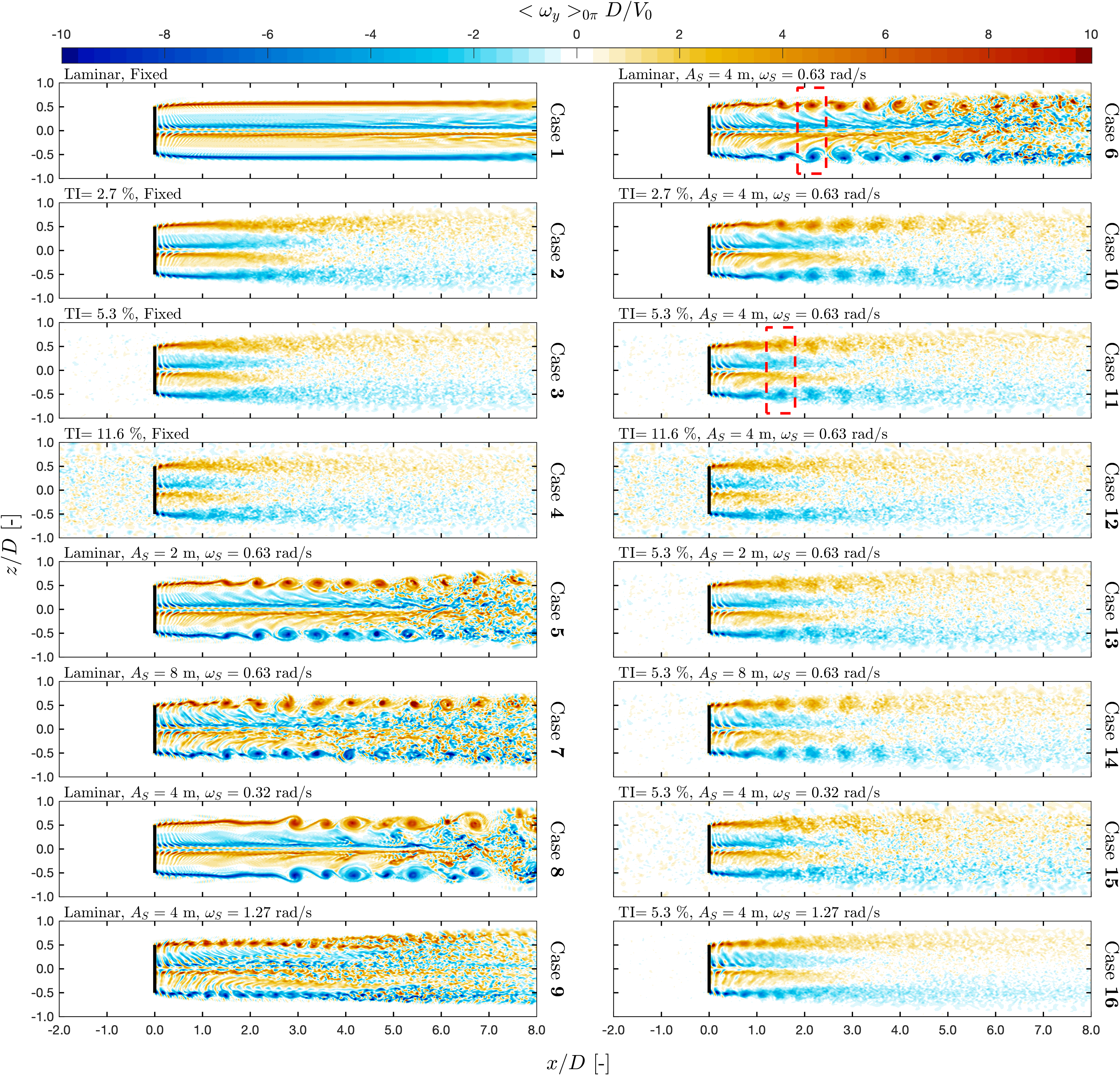
Figure 15: Fields of phase-locked averaged $y$-component vorticity $<\omega_{y}>_{0\pi}$ for all the 16 cases. Locations of the red dashed-line boxes for SIPCS of cases 6 & 11 were identical with Figure 12.

5.4.6 Momentum entrainment

With the analysis in Appendix E, streamwise momentum entrainment (recovery) $\partial\overline{uu}/\partial x$ was approximated as Equation 16, which contained four terms. The four terms were time-averaged pressure gradients $-\partial\overline{p}/\partial x$, vertical transport of mean streamwise momentum $-\overline{w}(\partial\overline{u}/\partial z)$, and two of the fluctuation (Reynolds Stress) terms $-\partial\overline{u^{\prime}w^{\prime}}/\partial z$ & $-\partial\overline{u^{\prime}u^{\prime}}/\partial x$. For brevity, only four representing cases were analyzed, which are laminar cases with fixed/surging rotor and turbulent cases with fixed/surging rotor (case 1, 3, 6, & 11), other cases are not presented since they shared very similar features. Contours of the four fields of the four cases are displayed in Figure 16.

$$\frac{\partial\overline{uu}}{\partial x}\simeq-\frac{2}{\rho}\frac{\partial{\overline{p}}}{\partial x}-2\overline{w}\frac{\partial\overline{u}}{\partial z}-2\frac{\partial\overline{u^{\prime}w^{\prime}}}{\partial z}-\frac{\partial\overline{u^{\prime}u^{\prime}}}{\partial x}$$ (16)

In the fields of $-\partial\overline{p}/\partial x$, clearly that the four cases experienced momentum losses to overcome the adverse pressure gradients due to the presence of rotor. However, after $x/D>1.5$, its effects on momentum were negligible, and the term did not aid momentum recovery at all.

For the contours of $-\overline{w}(\partial\overline{u}/\partial z)$, all the four cases had strips of negative values just behind the rotors, indicating the streamwise velocity of the flows became smaller as $x$ became bigger; this was due to that the flows with lower streamwise momentum were transported outward from the core of wake through the wake expansion process. Other than the negative strips just behind the rotors, the two turbulent cases also featured positive strips in contours of $-\overline{w}(\partial\overline{u}/\partial z)$ after the negative strips, and it was due to that the flows with higher momentum were brought from outer free-stream to the positive regions. Note that since the positive regions did not really go into area shaded by the rotor ($\lvert{z/D}\rvert\leq 0.5$), term $-\overline{w}(\partial\overline{u}/\partial z)$ was not the main source for the wake recoveries for these cases. For the laminar case with surging rotor, very interestingly, distinct contour with irregular patterns were found. This was related to the convection of flow structures with highly localized characteristics (SIPCS).

As for the contours of fluctuating term $-\partial\overline{u^{\prime}w^{\prime}}/\partial z$, it is clear that $-\partial\overline{u^{\prime}w^{\prime}}/\partial z$ was the main source term for momentum recoveries of the turbulent cases, since their values were much more significant compared to the other terms. Not surprisingly, the $-\partial\overline{u^{\prime}w^{\prime}}/\partial z$ field for laminar case with fixed rotor had values of zeroes almost everywhere, this was expected since that no recovery on $\overline{u}$ and very low values for TKE field were observed in the previous investigations. However, once again, laminar case with surging rotor had distinct pattern of $-\partial\overline{u^{\prime}w^{\prime}}/\partial z$ field; in general, seemed that there was a net positive momentum gain for the case, but its patterns were not as smooth as the turbulent cases.

Contours for term $-\partial\overline{u^{\prime}u^{\prime}}/\partial x$ showed that this term contributed much less compare to the other three terms, and thus it was not further analyzed. Though not shown in this paper, the other two terms related to $\partial\overline{uu}/\partial x$, $-\partial\overline{\left[(\nu+\nu_{T})(\partial u/\partial x+\partial u/\partial x)\right]}/\partial x$ & $-\partial\overline{\left[(\nu+\nu_{T})(\partial u/\partial z+\partial w/\partial x)\right]}/\partial z$, had further smaller values for their fields. Check Li Li (2023) for more detailed analysis.

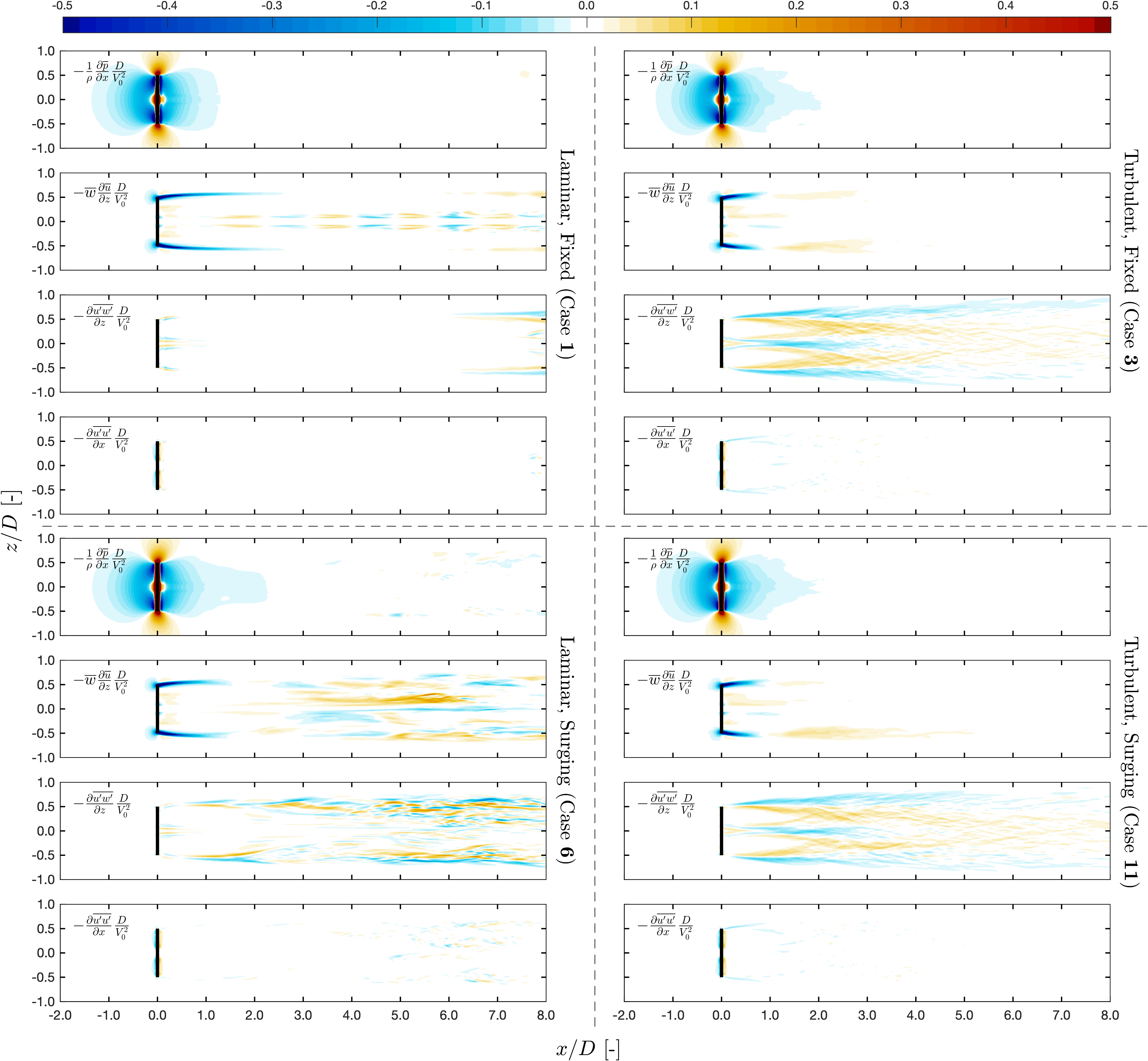
Figure 16: Fields of momentum entrainment ($\partial\overline{uu}/\partial x$) related fields ($-\overline{w}\frac{\partial\overline{u}}{\partial z},-\frac{\partial\overline{u^{\prime}u^{\prime}}}{\partial x},-\frac{\partial\overline{u^{\prime}w^{\prime}}}{\partial z},\&-\frac{1}{\rho}\frac{\partial{\overline{p}}}{\partial x}$). Four cases were presented, which are laminar fixed (top left), turbulent fixed (top right), laminar surging (bottom left), and turbulent surging (bottom right).

6 Expected and actual behaviors of $<C_{T}>$ & $<C_{P}>$

This section discusses the expected and actual behaviour of $<C_{T}>$ & $<C_{P}>$ with different surging settings; their time averaged values, asymmetries about the values of the fixed case, and stalling will be analyzed.

In Subsections 5.2, it had been shown that the curves of $<C_{T}>$ and $<C_{P}>$ seemed to be very similar with simple harmonic functions (for the cases without significant stalling); however, their mechanisms behind were actually rather complicated and simple analytical solutions were not easy to be formulated. To understand the behaviors of $<C_{T}>$ and $<C_{P}>$ for the full surging cycle, one should consider all the parameters that appeared in Equations 9 and 10, including surging velocity $V_{S}$, apparent normal velocity seen by the surging rotor’s airfoil sections (actuator line points) $V_{n,\mathrm{app}}$, $V_{\mathrm{rel}}$, $\phi$, $\alpha$, and airfoil polar data for $C_{l}$ & $C_{d}$.

6.1 Expected behaviors of $<C_{T}>$ & $<C_{P}>$

To begin with the analysis, instantaneous thrust and power conversion rates ($\xi_{C_{T}}$ & $\xi_{C_{P}}$) were introduced; they were linked to the instantaneous rotor thrust & power ($T$ & $P$) through the apparent inflow wind speed seen by the rotor $V_{0,\mathrm{app}}$ as in Equation 17. Notice that $C_{T}$ & $C_{P}$ ($\overline{C}_{T}$ & $\overline{C}_{P}$) in this paper were linked to $T$ & $P$ ($\overline{T}$ & $\overline{P}$) through $V_{0}$, which were different from $\xi_{C_{T}}$ & $\xi_{C_{P}}$.

$$T=\xi_{C_{T}}V_{0,\mathrm{app}}^{2},\qquad P=\xi_{C_{P}}V_{0,\mathrm{app}}^{3}$$ (17)

If $\xi_{C_{T}}$ & $\xi_{C_{P}}$ were considered to be fixed (constants) and effects of dynamic inflow were negligible throughout the surging cycle, both the values for time-averaged thrust and power coefficients ($\overline{C}_{T}$ & $\overline{C}_{P}$) for the surging cases should be greater than the fixed case, due to the inequalities shown in Equations 18 and 19 (Johlas et al. Johlas et al. (2021) had done a similar analysis). And with these facts, values of $\overline{C}_{T}$ and $\overline{C}_{P}$ should be bigger for cases with larger $\mathbb{V}$. However, both $\overline{C}_{T}$ and $\overline{C}_{P}$ did not comply the hypothesis as can be seen in Figure 5, where $\overline{C}_{T}$ of the surging cases even dropped, and it dropped more with larger $\mathbb{V}$. This underlined that $\xi_{C_{T}}$ and $\xi_{C_{P}}$ were not constants during the surging cycle, and how $f_{n}$ & $f_{\theta}$ were obtained for every actuator line points should be closely looked into (Equations 9 & 10). Nevertheless, as $V_{0,\mathrm{app}}$ were influenced by surging motions in the simulations, the operational conditions (such as $\Omega$) did not adjust accordingly, making the rotor operate in sub-optimal conditions, and thus affecting $\xi_{C_{T}}$ and $\xi_{C_{P}}$ (where $\xi_{C_{P}}$ was expected to drop). Once again, note that the values of reference velocity for $\overline{C}_{T}$ & $\overline{C}_{P}$ were both based on $V_{0}$ (fixed value) for this paper, not $V_{0,\mathrm{app}}$.

$$\frac{1}{T_{S}}\int_{0}^{T_{S}}\xi_{C_{T}}V_{0,\mathrm{app}}^{2}\mathrm{d}t=\frac{1}{T_{S}}\int_{0}^{T_{S}}\xi_{C_{T}}V_{0}^{2}(1-\mathbb{V}\cos\omega_{S}t)^{2}\mathrm{d}t\hskip 5.0pt{\huge>}\hskip 5.0pt\xi_{C_{T}}V_{0}^{2},\quad\mathrm{for}\quad 0<\mathbb{V}<1$$ (18)

$$\frac{1}{T_{S}}\int_{0}^{T_{S}}\xi_{C_{P}}V_{0,\mathrm{app}}^{3}\mathrm{d}t=\frac{1}{T_{S}}\int_{0}^{T_{S}}\xi_{C_{P}}V_{0}^{3}(1-\mathbb{V}\cos\omega_{S}t)^{3}\mathrm{d}t\hskip 5.0pt{\huge>}\hskip 5.0pt\xi_{C_{P}}V_{0}^{3},\quad\mathrm{for}\quad 0<\mathbb{V}<1$$ (19)

6.2 Actual behaviors of $<C_{T}>$ & $<C_{P}>$

If looking closer to the the curves of $<C_{T}>$ and $<C_{P}>$ for the surging cases, for example in Figures 7(b) & 7(c), one can find that as $V_{S}=0$ m/s ($<t>/T_{\Omega}=0.5$ or $1.5$), values for $<C_{T}>$ and $<C_{P}>$ were both very close of the fixed case (neutral values), suggesting hysteresis (dynamic inflow) effects were weak (see Figure 9(c) for more details about hysteresis effects). Moreover, even though the curves looked quite like sinusoidal, their fluctuations were not symmetry about the neutral values, especially for $<C_{T}>$. Clearly that with the neutral values as the base points, the under-shoots of $<C_{T}>$ were larger than the over-shoots, and this also reflected in lower values of $\overline{C}_{T}$ (see Figure 5). As for $\overline{C}_{P}$, its values for fixed and surging cases considered in this paper were similar (slightly higher for cases with $\mathbb{V}=0.11$ & $0.22$ but slightly smaller for cases with $\mathbb{V}=0.44$).

The different behaviors of $\overline{C}_{T}$ and $\overline{C}_{P}$ as comparing to the neutral values could be explained by that both the inflow angle $\phi$ and angle of attack $\alpha$ were varying during the surging cycles. As can be seen in Equation 10, a larger $V_{n,\mathrm{app}}$ would result in a larger $\phi$ and thus a larger $\alpha$, and a larger $\alpha$ would lead to a larger lift force $\boldsymbol{L}$ in general (if stalling did not occur). Moreover, generally the larger $\boldsymbol{L}$ would end up in larger $T$ & $P$, since they both directly related to $\boldsymbol{L}$. However, $\phi$ was also changing as $V_{n,\mathrm{app}}$ varied, and note that $\boldsymbol{L}$ can be decomposed into $\hat{\boldsymbol{e}}_{n}$ & $\hat{\boldsymbol{e}}_{\theta}$ (Equation 20), where they were the normal (thrust) component and tangential (torque) component. With basic trigonometry, a bigger $\phi$ would lead to a smaller $\cos{\phi}$ but larger $\sin{\phi}$, projecting $\boldsymbol{L}$ less to the normal component (contributed to $T$) but more to the tangential component (contributed to $P$). Therefore, the increases in $C_{T}$ due to the enlargement of $V_{n,\mathrm{app}}$ were less than $C_{P}$. While as $V_{n,\mathrm{app}}<V_{{n}}$ ($V_{0,\mathrm{app}}<V_{{0}}$), opposite situations occurred, $C_{T}$ dropped less while $C_{P}$ dropped more. However, according to Equations 18 and 19, it was reasonable that windows when $V_{n,\mathrm{app}}>V_{{n}}$ were more important when it came to the time-averaged values of $\overline{C}_{T}$ & $\overline{C}_{P}$ due to the weighting of $V_{0,\mathrm{app}}^{2}$ & $V_{0,\mathrm{app}}^{3}$.

Besides the analysis about how $T$ & $P$ may behave during the surging cycle just carried out above, it should be noticed that the rotor would operate under rather suboptimal conditions as $V_{S}\neq 0$ (since $\Omega$ was fixed), and stalling would further lower the values for $C_{T}$ and $C_{P}$ (see Section 5.3). After combining all these together, it was reasonable to have results of smaller $\overline{C}_{T}$ for surging cases than the fixed cases, while similar $\overline{C}_{P}$ for fixed and surging cases (see Figure 5).

$$\boldsymbol{L}=\lvert\boldsymbol{L}\rvert\cos{\phi}\hskip 3.0pt\hat{\boldsymbol{e}}_{n}+\lvert\boldsymbol{L}\rvert\sin{\phi}\hskip 3.0pt\hat{\boldsymbol{e}}_{\theta}$$ (20)

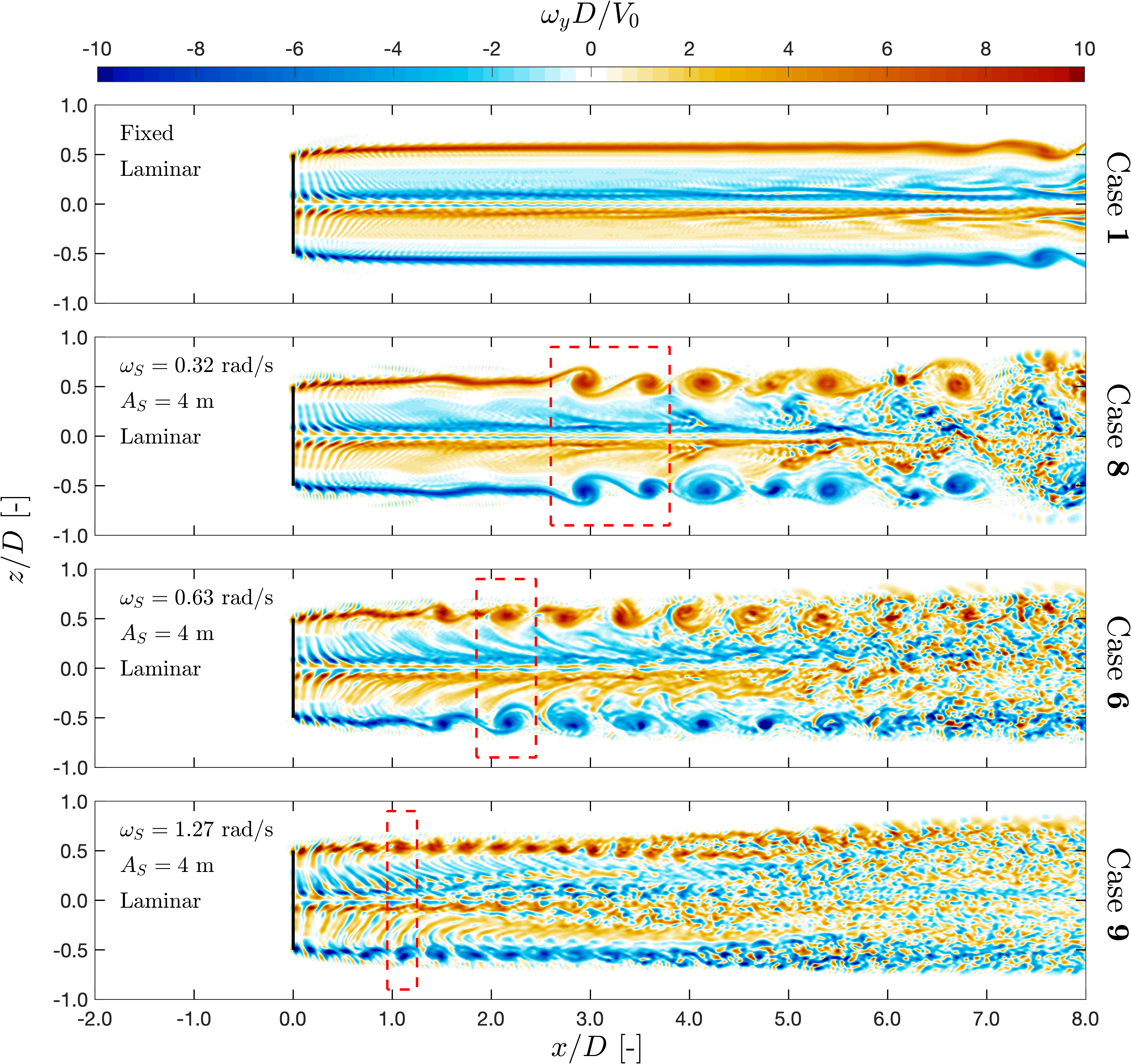
Figure 17: Instantaneous $\omega_{y}$ fields (as $\phi_{S}=0\pi$ or $\phi_{\Omega}=0\pi$) depicting the Surging Induced Periodic Coherent Structures (SIPCS) with different $\omega_{S}$. Boxes with red-dashed line enclosed the vortical structures generated within a surging cycle. Form top to bottom: Fixed, $\omega_{S}=0.32$ rad/s, $\omega_{S}=0.63$ rad/s and $\omega_{S}=1.27$ rad/s.

7 Further discussions about SIPCS

As the $<u>_{0\pi}$ and $<\omega_{y}>_{0\pi}$ fields displayed in Sections 5.4, surging cases had distinct periodic coherent structures (SIPCS) in their wakes, especially for the cases with laminar inflow conditions. As can be seen in Figure 15, the modes of the SIPCS were mainly dominated by surging frequencies $\omega_{S}$, while surging amplitudes $A_{S}$ had less influences for the cases considered. Figure 17 illustrates the vortical (coherent) structures with instantaneous $\omega_{y}$ fields (at instant where $\phi_{S}=0\pi$ & $\phi_{\Omega}=0\pi$) for laminar cases of $\omega_{S}$ being $0.32$, $0.63$, and $1.27$ rad/s along with a fixed case (cases 1, 6, 8, & 9). In the figure, the boxes of red dashed-line indicate the vortical structures formed within a surging cycle, and it can be seen that the vortical structures for the three surging cases were formed through merging of tip-vorticies with rolling-up process. The merging processes were triggered since the inter-distances between tip-vorticies were varied during a surging cycle, which brought up the imbalance of inductance forces among them. It is worth noting that each pair of the vortical structures appeared in the figures are actually a ring since the wakes were $3$-dimensional, and for the cases of $\omega_{S}=0.63$ rad/s & $\omega_{S}=1.27$ rad/s, each pair of the vortical structure corresponded to a complete surging cycle; as for the case with $\omega_{S}=0.32$ rad/s, a completed surging cycle corresponded to two pairs (rings) of vortical structures, with a pair stronger and another weaker.

8 Conclusions and outlooks

In this paper, comprehensive investigations of the influences of inflow turbulence intensities (TI), surging amplitudes ($A_{S}$) and surging frequencies ($\omega_{S}$) were conducted with a surging full-scale horizontal-axis wind turbine rotor.

For cases with a surging rotor under laminar inflows, distinct periodic flow structures related to surging motions (SIPCS) were found in their wakes immediately through the instantaneous fields. These structures were formed through the merging of the tip-vorticies, and their repeating rates were as $\omega_{S}$. While for the surging cases under turbulent inflows, surging related periodic structures were not found with the instantaneous fields, and they were only clearly revealed after phase-locked averaged fields; cases with lower inflow TI or larger $A_{S}$ would have clearer patterns for the surging related periodic structures. Regarding the wake recovery rates, the mean disk-averaged streamwise velocity of the surging cases could be more than $30\%$ larger than the fixed cases at $x/D=8$ as the inflow conditions were laminar, while the surging cases under turbulent inflow conditions would only have about $0.5\sim 2\%$ gain in mean disk-averaged streamwise velocity ($\overline{u}_{\mathrm{Disk}}$) compared to the fixed cases at the same position. And for both the laminar and turbulent cases, the increases in mean disk-averaged streamwise velocity were more significant with stronger surging settings with the considered surging motions.

Generally, inflow TI had little effect on time-averaged and cycle-averaged rotor performances. However, surging settings considered in this paper affected noticeably on $\overline{C}_{T}$ but only slightly on $\overline{C}_{P}$. More specifically, for the cases considered in this paper, before severe stalling occurred, stronger surging settings (with larger $\mathbb{V}$) would bring lower $\overline{C}_{T}$ with slightly higher $\overline{C}_{P}$, while for the cases with severe stalling (cases with $\mathbb{V}=0.44$), $\overline{C}_{T}$ was significantly lower than the fixed case while $\overline{C}_{P}$ was slightly lower. As for the hysteresis (dynamic inflow) effects for surging cases, they were quite mild for the cases considered.

For future work, cases with similar simulation setups could be tested with different type of motions, such as rolling and pitching, or even combined. Also, cases with multiple FOWT (floating offshore wind turbine) rotors in motions can be tested as well, these cases may aid the understanding about the modes of wake interactions among FOWTs, and to see how the (surging) motions affect the power outputs of wind turbine rotors in the wind farm level.

Appendix A Convergence Tests

Figure 18 displays the results of brief convergence tests for $\overline{u}$, $<u>_{0\pi}$, $\sigma_{u}$, & $<\sigma_{u}>_{0\pi}$. The probing point was located at the tip $z=D/2$, and the streamwise position was $x/D=3$. The windows for calculating the statistics had been described in Subsection 4.2. For more information, see Li Li (2023).

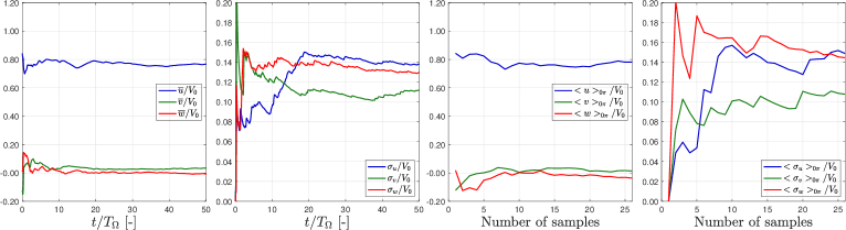
Figure 18: Convergence tests of outputs sampled at $x/D=3$, $z=D/2$.

Appendix B Grid independence test

A brief grid independence test was carried out. It was done with three resolutions, and they were tested with a surging rotor ($A_{S}=4$ m & $\omega_{S}=0.63$ rad/s) under laminar inflow conditions. The resolutions for Level 4 of the three cases were $\Delta/D=1.25/80$ (coarse, $5.6$M cells), $\Delta/D=1.0/80$ (medium, $10.9$M cells), and $\Delta/D=0.8/80$ (fine, $18.8$M cells). Note that the absolute value of $\varepsilon$ was kept as $D/40$. Their results are presented in Figure 19, showing that the results were not sensitive to grid resolution. Though it seemed the results of coarse were already quite similar to the other configurations, medium was chosen for the simulations. The choice was based on considering the best practice established by the proceeding works Sarlak et al. (2015); Martínez-Tossas et al. (2015) for using LES with ALM to model wakes of wind turbine, and $10.9$M cells was rather affordable with the given computational resources.

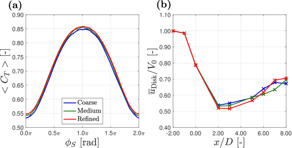
Figure 19: Grid sensitivity tests about the cycle-averaged rotor performances ($<C_{T}>$) and integral wake characteristics ($\overline{u}_{\mathrm{Disk}}$).

Appendix C Auxiliary cases

Table 5 lists out the basic settings and results for the six auxiliary cases. These auxiliary cases were tested with different inflow velocity $V_{0}$ under laminar inflow conditions, and the values of these $V_{0}$ corresponded to the maximum and minimum $V_{0,\mathrm{app}}$ for each surging settings appeared in Table 3. Results of these cases were utilized in Figure 9(c) to assess the hysteresis (dynamic inflow) effects due to the surging motions of rotor.

Table 5: The basic settings and results for the auxiliary cases with different $V_{0}$ but identical rotational frequency ($\Omega=1.26$ rad/s) of a single fixed NREL 5MW rotor. Note that $V_{\mathrm{ref}}$ for calculating $\overline{C}_{T}$ & $\overline{C}_{P}$ are based on $V_{\mathrm{ref}}=V_{0,\mathrm{rated}}=11.4$ m/s.

Case	TI [$\%$]	$V_{0}/$ [m/s]	$V_{0}/V_{0,\mathrm{rated}}$	$\overline{C}_{T}$	$\overline{C}_{P}$
17	Lam.	$6.33$	$0.56$	$0.330$	$0.076$
18	Lam.	$8.67$	$0.78$	$0.538$	$0.264$
19	Lam.	$10.13$	$0.90$	$0.640$	$0.388$
20	Lam.	$12.67$	$1.11$	$0.801$	$0.651$
21	Lam.	$13.93$	$1.22$	$0.859$	$0.783$
22	Lam.	$16.47$	$1.44$	$0.856$	$0.846$

Appendix D Profile of $\alpha_{\mathrm{{stall}}}$ for NREL 5MW

Figure 20 presents the $\alpha_{\mathrm{stall}}$ profile along the blade span of NREL 5MW baseline turbine. Note that the airfoil sections were not the same and thus $\alpha_{\mathrm{stall}}$ varied along the blade.

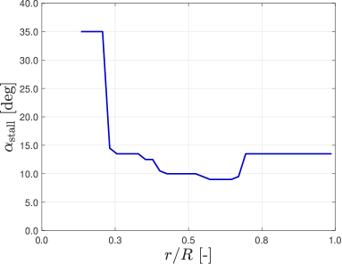
Figure 20: Profile of $\alpha_{\mathrm{stall}}$ for NREL 5MW baseline turbine.

Appendix E Momentum Entertainment

Term $\partial\overline{uu}/\partial x$, which has the physical meaning of gain of $x$-momentum of the flow along $x$-direction, can be written as Equation 21 by applying chain rule and Reynolds decomposition ($u=\overline{u}+u^{\prime}$). And for the wake regions being free from the projected body force fields of actuator lines, $x$-component of the filtered Navier-Stokes equations (Equation 7 right) can be written as Equation 22. By taking the time average of Equation 22, Equation 23 was arrived. After implementing Reynolds decomposition, chain-rule, and (filtered) continuity equation (Equation 7 left), Equation 23 can be re-written as Equation 28 through the steps from Equations 24 to 27. Plugging Equation 21 into Equation 28, Equation 29 was arrived.

$$\frac{\partial\overline{uu}}{\partial x}=\frac{\partial}{\partial x}\left(\overline{(\overline{u}+u^{\prime})(\overline{u}+u^{\prime})}\right)=\frac{\partial}{\partial x}\left(\overline{\overline{u}\hskip 2.0pt\overline{u}+\underbrace{2\overline{u}u^{\prime}}_{=0}+u^{\prime}u^{\prime}}\right)=\left(\frac{\partial\overline{u}\hskip 2.0pt\overline{u}}{\partial x}+\frac{\partial\overline{u^{\prime}u^{\prime}}}{\partial x}\right)=2\overline{u}\frac{\partial\overline{u}}{\partial x}+\frac{\partial\overline{u^{\prime}u^{\prime}}}{\partial x}$$ (21)

$$\frac{\partial{u}}{\partial t}+{u}\frac{\partial{u}}{\partial x}+{v}\frac{\partial{u}}{\partial y}+{w}\frac{\partial{u}}{\partial z}=-\frac{1}{\rho}\frac{\partial{p}}{\partial x}+\frac{\partial}{\partial x}\left[(\nu+\nu_{T})\left(\frac{\partial{u}}{\partial x}+\frac{\partial{u}}{\partial x}\right)\right]\\ +\frac{\partial}{\partial y}\left[(\nu+\nu_{T})\left(\frac{\partial{u}}{\partial y}+\frac{\partial{v}}{\partial x}\right)\right]+\frac{\partial}{\partial z}\left[(\nu+\nu_{T})\left(\frac{\partial{u}}{\partial z}+\frac{\partial{w}}{\partial x}\right)\right]$$ (22)

$$\overline{{u}\frac{\partial{u}}{\partial x}}+\overline{{v}\frac{\partial{u}}{\partial y}}+\overline{{w}\frac{\partial{u}}{\partial z}}=-\frac{1}{\rho}\frac{\partial{\overline{p}}}{\partial x}+\overline{\frac{\partial}{\partial x}\left[(\nu+\nu_{T})\left(\frac{\partial{u}}{\partial x}+\frac{\partial{u}}{\partial x}\right)\right]}\\ +\overline{\frac{\partial}{\partial y}\left[(\nu+\nu_{T})\left(\frac{\partial{u}}{\partial y}+\frac{\partial{v}}{\partial x}\right)\right]}+\overline{\frac{\partial}{\partial z}\left[(\nu+\nu_{T})\left(\frac{\partial{u}}{\partial z}+\frac{\partial{w}}{\partial x}\right)\right]}$$ (23)

$$\left(\overline{\frac{\partial{uu}}{\partial x}}-\overline{u\frac{\partial u}{\partial x}}\right)+\left(\overline{\frac{\partial{uv}}{\partial y}}-\overline{u\frac{\partial v}{\partial y}}\right)+\left(\overline{\frac{\partial{uw}}{\partial z}}-\overline{u\frac{\partial w}{\partial z}}\right)=-\frac{1}{\rho}\frac{\partial{\overline{p}}}{\partial x}\\ +\overline{\frac{\partial}{\partial x}\left[(\nu+\nu_{T})\left(\frac{\partial{u}}{\partial x}+\frac{\partial{u}}{\partial x}\right)\right]}+\overline{\frac{\partial}{\partial y}\left[(\nu+\nu_{T})\left(\frac{\partial{u}}{\partial y}+\frac{\partial{v}}{\partial x}\right)\right]}+\overline{\frac{\partial}{\partial z}\left[(\nu+\nu_{T})\left(\frac{\partial{u}}{\partial z}+\frac{\partial{w}}{\partial x}\right)\right]}$$ (24)

$$\left(\overline{\frac{\partial{uu}}{\partial x}}+\overline{\frac{\partial{uv}}{\partial y}}+\overline{\frac{\partial{uw}}{\partial z}}\right)-\overline{u\underbrace{\left(\frac{\partial u}{\partial x}+\frac{\partial v}{\partial y}+\frac{\partial w}{\partial z}\right)}_{\mathrm{continuity}=0}}=-\frac{1}{\rho}\frac{\partial{\overline{p}}}{\partial x}\\ +\overline{\frac{\partial}{\partial x}\left[(\nu+\nu_{T})\left(\frac{\partial{u}}{\partial x}+\frac{\partial{u}}{\partial x}\right)\right]}+\overline{\frac{\partial}{\partial y}\left[(\nu+\nu_{T})\left(\frac{\partial{u}}{\partial y}+\frac{\partial{v}}{\partial x}\right)\right]}+\overline{\frac{\partial}{\partial z}\left[(\nu+\nu_{T})\left(\frac{\partial{u}}{\partial z}+\frac{\partial{w}}{\partial x}\right)\right]}$$ (25)

$$\frac{\partial{}}{\partial x}\left(\overline{u}\hskip 2.0pt\overline{u}+\overline{u^{\prime}u^{\prime}}\right)+\frac{\partial{}}{\partial y}\left(\overline{u}\hskip 2.0pt\overline{v}+\overline{u^{\prime}v^{\prime}}\right)+\frac{\partial{}}{\partial z}\left(\overline{u}\hskip 2.0pt\overline{w}+\overline{u^{\prime}w^{\prime}}\right)=-\frac{1}{\rho}\frac{\partial{\overline{p}}}{\partial x}\\ +\overline{\frac{\partial}{\partial x}\left[(\nu+\nu_{T})\left(\frac{\partial{u}}{\partial x}+\frac{\partial{u}}{\partial x}\right)\right]}+\overline{\frac{\partial}{\partial y}\left[(\nu+\nu_{T})\left(\frac{\partial{u}}{\partial y}+\frac{\partial{v}}{\partial x}\right)\right]}+\overline{\frac{\partial}{\partial z}\left[(\nu+\nu_{T})\left(\frac{\partial{u}}{\partial z}+\frac{\partial{w}}{\partial x}\right)\right]}$$ (26)

$${\overline{u}}\frac{\partial\overline{u}}{\partial x}+\overline{v}\frac{\partial\overline{u}}{\partial y}+\overline{w}\frac{\partial\overline{u}}{\partial z}+{\overline{u}}\underbrace{\left(\frac{\partial\overline{u}}{\partial x}+\frac{\partial\overline{v}}{\partial y}+\frac{\partial\overline{w}}{\partial z}\right)}_{=0}+\frac{\partial\overline{u^{\prime}u^{\prime}}}{\partial x}+\frac{\partial\overline{u^{\prime}v^{\prime}}}{\partial y}+\frac{\partial\overline{v^{\prime}w^{\prime}}}{\partial z}=-\frac{1}{\rho}\frac{\partial{\overline{p}}}{\partial x}\\ +\overline{\frac{\partial}{\partial x}\left[(\nu+\nu_{T})\left(\frac{\partial{u}}{\partial x}+\frac{\partial{u}}{\partial x}\right)\right]}+\overline{\frac{\partial}{\partial y}\left[(\nu+\nu_{T})\left(\frac{\partial{u}}{\partial y}+\frac{\partial{v}}{\partial x}\right)\right]}+\overline{\frac{\partial}{\partial z}\left[(\nu+\nu_{T})\left(\frac{\partial{u}}{\partial z}+\frac{\partial{w}}{\partial x}\right)\right]}$$ (27)

$${\overline{u}}\frac{\partial\overline{u}}{\partial x}+\overline{v}\frac{\partial\overline{u}}{\partial y}+\overline{w}\frac{\partial\overline{u}}{\partial z}+\frac{\partial\overline{u^{\prime}u^{\prime}}}{\partial x}+\frac{\partial\overline{u^{\prime}v^{\prime}}}{\partial y}+\frac{\partial\overline{v^{\prime}w^{\prime}}}{\partial z}=-\frac{1}{\rho}\frac{\partial{\overline{p}}}{\partial x}\\ +\overline{\frac{\partial}{\partial x}\left[(\nu+\nu_{T})\left(\frac{\partial{u}}{\partial x}+\frac{\partial{u}}{\partial x}\right)\right]}+\overline{\frac{\partial}{\partial y}\left[(\nu+\nu_{T})\left(\frac{\partial{u}}{\partial y}+\frac{\partial{v}}{\partial x}\right)\right]}+\overline{\frac{\partial}{\partial z}\left[(\nu+\nu_{T})\left(\frac{\partial{u}}{\partial z}+\frac{\partial{w}}{\partial x}\right)\right]}$$ (28)

$$\frac{\partial\overline{uu}}{\partial x}=2{\overline{u}}\frac{\partial\overline{u}}{\partial x}+\frac{\partial\overline{u^{\prime}u^{\prime}}}{\partial x}=-2\overline{v}\frac{\partial\overline{u}}{\partial y}-2\overline{w}\frac{\partial\overline{u}}{\partial z}-\frac{\partial\overline{u^{\prime}u^{\prime}}}{\partial x}-2\frac{\partial\overline{u^{\prime}v^{\prime}}}{\partial y}-2\frac{\partial\overline{u^{\prime}w^{\prime}}}{\partial z}-\frac{2}{\rho}\frac{\partial{\overline{p}}}{\partial x}\\ +2\overline{\frac{\partial}{\partial x}\left[(\nu+\nu_{T})\left(\frac{\partial{u}}{\partial x}+\frac{\partial{u}}{\partial x}\right)\right]}+2\overline{\frac{\partial}{\partial y}\left[(\nu+\nu_{T})\left(\frac{\partial{u}}{\partial y}+\frac{\partial{v}}{\partial x}\right)\right]}+2\overline{\frac{\partial}{\partial z}\left[(\nu+\nu_{T})\left(\frac{\partial{u}}{\partial z}+\frac{\partial{w}}{\partial x}\right)\right]}$$ (29)

This paper focused on $y=0$ plane to study momentum entrainment. Due to the fact that the wake should be close to axis-symmetric (tower, floor, and wind shear were not considered), terms related to $\partial/\partial y$ were assumed to be negligible and thus not considered, making Equation 29 become Equation 30. Moreover, effects of the terms related to $\nu$ and $\nu_{T}$ (shear terms) were relatively much smaller when comparing to the other four terms, and thus they may be also neglected (check Li Li (2023)). With these simplifications, term $\partial\overline{uu}/\partial x$ was left with the four terms in Equation 31, which are the terms in Figure 16.

$$\frac{\partial\overline{uu}}{\partial x}\simeq-2\overline{w}\frac{\partial\overline{u}}{\partial z}-\frac{\partial\overline{u^{\prime}u^{\prime}}}{\partial x}-2\frac{\partial\overline{u^{\prime}w^{\prime}}}{\partial z}-\frac{2}{\rho}\frac{\partial{\overline{p}}}{\partial x}\\ +2\overline{\frac{\partial}{\partial x}\left[(\nu+\nu_{T})\left(\frac{\partial{u}}{\partial x}+\frac{\partial{u}}{\partial x}\right)\right]}+2\overline{\frac{\partial}{\partial z}\left[(\nu+\nu_{T})\left(\frac{\partial{u}}{\partial z}+\frac{\partial{w}}{\partial x}\right)\right]}$$ (30)

$$\frac{\partial\overline{uu}}{\partial x}\simeq-2\overline{w}\frac{\partial\overline{u}}{\partial z}-\frac{\partial\overline{u^{\prime}u^{\prime}}}{\partial x}-2\frac{\partial\overline{u^{\prime}w^{\prime}}}{\partial z}-\frac{2}{\rho}\frac{\partial{\overline{p}}}{\partial x}$$ (31)