Cosmology with Galaxy Photometry Alone

Abstract

We present the first cosmological constraints using only the observed photometry of galaxies. Villaescusa-Navarro et al. (2022b) recently demonstrated that the internal physical properties of a single simulated galaxy contain a significant amount of cosmological information. These physical properties, however, cannot be directly measured from observations. In this work, we present how we can go beyond theoretical demonstrations to infer cosmological constraints from actual galaxy observables (e.g. optical photometry) using neural density estimation and the CAMELS suite of hydrodynamical simulations. We find that the cosmological information in the photometry of a single galaxy is limited. However, we combine the constraining power of photometry from many galaxies using hierarchical population inference and place significant cosmological constraints. With the observed photometry of $\sim$20,000 NASA-Sloan Atlas galaxies, we constrain $\Omega_{m}=0.323^{+0.075}_{-0.095}$ and $\sigma_{8}=0.799^{+0.088}_{-0.085}$.

1 Introduction

In recent work, Villaescusa-Navarro et al. (2022b) showed that it is possible to place cosmological constraints by utilizing only the internal properties of a single simulated galaxy. They used galaxies from 2,000 state-of-the-art hydrodynamical simulations with different cosmologies and astrophysical models from the CAMELS project (Villaescusa-Navarro et al., 2021, 2022a) to train moment networks (Jeffrey & Wandelt, 2020) that predict cosmological parameters from galaxy properties. With only a handful of galaxy properties, including stellar mass ($M_{*}$), stellar metallicity ($Z_{*}$), and maximum circular velocity ($V_{\rm max}$), they were able to constrain $\Omega_{m}$ to 10% precision with a single galaxy. They found similar constraining power for galaxies simulated using the subgrid physics models of the IllustrisTNG (Pillepich et al., 2018; Weinberger et al., 2018) and SIMBA (Davé et al., 2019) simulations. Echeverri et al. (2023) reached similar conclusions using yet another subgrid physics model from Astrid (Ni et al., 2022; Bird et al., 2022).

According to Villaescusa-Navarro et al. (2021), the cosmological information is derived from the imprint of $\Omega_{m}$ on the dark matter content of galaxies that affects galaxy properties in a way distinct from astrophysical processes. Because $\Omega_{b}$ is fixed in CAMELS, which is justified by the tight constraints from Big Bang Nucleosynthesis (Aver et al., 2015; Cooke et al., 2018; Schöneberg et al., 2019), galaxy properties actually measure the baryon fraction, $\Omega_{b}/\Omega_{m}$. For instance, $V_{\rm max}$ measures the depth of the total matter gravitational potential while other properties like $M_{*}$ and $Z_{*}$ measures the mass in baryons, so together they constrain the ratio $\Omega_{b}/\Omega_{m}$. In fact, a similar approach was already used by White et al. (1993) to constrain $\Omega_{b}/\Omega_{m}$ using galaxy clusters.

Despite promising signs that they may be useful cosmological probes, galaxy properties themselves are not actually observable. They are derived quantities that are typically inferred from photometry or spectra and require modeling the spectral energy distribution (SED) or emission lines (see Conroy, 2013, for a review). In this work, we go beyond the theoretical considerations of previous works and infer cosmological parameters from actual galaxy observables — optical photometry. We leverage a simulation-based inference method that employs neural density estimation (NDE) to estimate the posterior of cosmological parameters given galaxy photometry, similar to the approach of Hahn & Melchior (2022). Furthermore, since we expect a limited amount of cosmological information from the photometry of a single galaxy, we present a hierarchical population inference approach for inferring the posterior of cosmological parameters from the photometry of multiple galaxies. Lastly, we present the cosmological constraints derived from applying this approach to the photometry of $\sim$20,000 SDSS galaxies from the NASA-Sloan Atlas.

2 Observations: NASA-Sloan Atlas

In this work, we analyze galaxy photometry from the NASA-Sloan Atlas (hereafter NSA). The NSA provides photometry of $z<0.05$ galaxies observed by the Sloan Digital Sky Survey (SDSS; Aihara et al., 2011) Data Release 8 with improved background subtraction (Blanton et al., 2011). We use optical $g$, $r$, $i$, $z$ band absolute magnitudes derived using kcorrect (Blanton & Roweis, 2007), assuming a Chabrier (2003) initial mass function (IMF).

Out of the full NSA sample, we focus on luminous galaxies with $-18>M_{r}>-22$ that have precisely measured photometry: magnitude uncertainties below $(\sigma_{g},\sigma_{r},\sigma_{i})<0.022$ and $\sigma_{z}<0.04$. In addition, we impose color cuts, specified in Table 1, to ensure that our observed sample is contained within the photometric distribution (i.e. support) of our simulated galaxies (Section 3). These cuts exclude NSA galaxies outside of the central 68 percentile range of the $g-r$, $g-i$, $g-z$, $r-i$, $r-z$, $i-z$ simulated galaxy color distributions. The color cuts also remove NSA galaxies that potentially have observational artifacts or problematic photometry. We mark the 95^th percentile contour of our NSA subsample in Figure 1 (orange dot-dashed). In total, we use 22,338 NSA galaxies.

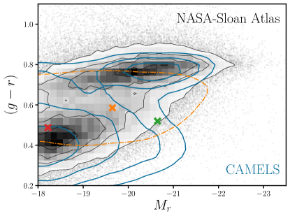
Figure 1: Color-magnitude distribution, $(g-r)-M_{r}$, of observed galaxies from the NSA (black) and simulated galaxies from CAMELS-TNG (blue). Overall, the distributions of NSA and CAMELS-TNG galaxies are in good agreement. The distribution for CAMELS-TNG is significantly broader because its galaxies are simulated using a wide range of cosmological and baryonic feedback parameters. We mark the 95^th percentile contour of the NSA subsample of 22,338 galaxies analyzed in this work (orange dot dashed; Section 2) along with three arbitrarily selected galaxies from this sample (crosses).

3 Forward Model: CAMELS

We use simulated galaxies from CAMELS, a suite of hydrodynamical simulations constructed over a wide range of cosmological and hydrodynamical parameters. In particular, we use the 1,000 hydrodynamical simulations constructed using the state-of-the-art IllustrisTNG model (CAMELS-TNG). The simulations are generated with different cosmological parameters, $\Omega=\{\Omega_{m},\sigma_{8}\}$, and baryonic feedback parameters, $\mathcal{B}=\{A_{\rm SN1},A_{\rm SN2},A_{\rm AGN1},A_{\rm AGN2}\}$, arranged in a latin hypercube. $A_{\rm SN1}$ and $A_{\rm SN2}$ represent the normalization factors for the galactic wind flux and speed; $A_{\rm AGN1}$ and $A_{\rm AGN2}$ represent the normalization factors for the energy output and specific energy of AGN feedback.

In the 1,000 simulations, there are a total of $\sim$700,000 galaxies with $M_{*}>2\times 10^{8}M_{\odot}/h$. The individual simulations, however, have different numbers of galaxies. For instance, simulations constructed at higher $\Omega_{m}$ values generally have more galaxies. This parameter dependence means that the $\Omega$ and $\mathcal{B}$ distribution of the CAMELS galaxies are non-uniform when considering individual galaxies. We correct for this implicit prior by randomly selecting 100 galaxies from each simulation. This imposes a uniform prior on $\Omega$ and $\mathcal{B}$ and leaves us with a total of 100,000 CAMELS-TNG galaxies.

Because our aim is to analyze the observed photometry of NSA galaxies, we forward model photometry for the simulated galaxies. CAMELS-TNG provides synthetic unattenuated stellar photometry for each simulated galaxy. For each galaxy, the SED of every star particle in its host subhalo is modeled as a single-burst simple stellar population using stellar population synthesis (SPS) based on the recorded birth time, metallicity, and mass. The SPS uses FSPS (Conroy et al., 2009), Padova isochrones, MILES stellar library, and assumes a Chabrier (2003) IMF. Then the SEDs of the star particles are combined to produce the unattenuated SED of the galaxy and convolved with SDSS $g$, $r$, $i$, $z$-band photometric bandpasses to produce the unattenuated photometry.

Next, we impose dust attenuation on the photometry. In the original TNG300 simulation, synthetic dust attenuated photometry was computed using a dust model based on the metal content of the neutral gas distribution in and around each galaxy (Nelson et al., 2018). We emulate this dust attenuation method in our forward model. First, we compile the unattenuated and attenuated SDSS $g$, $r$, $i$, $z$-band magnitudes for all TNG300 galaxies. We calculate the attenuation on the photometry by taking the difference between the unattenuated and attenuated magnitudes of the TNG300 galaxies. Then, for each CAMELS-TNG galaxy, we assign the attenuation of the TNG300 galaxy with the closest unattenuated photometry based on L2 norm. Each TNG300 galaxy has 12 sets of attenuated magnitudes, which correspond to the different observer viewing angles. We randomly select one of the viewing angles in the assignment. We attenuate the CAMELS-TNG galaxies by the assigned attenuation to get the attenuated photometry: $X_{i}$.

Finally, we add noise, $\sigma_{X}$, to the synthetic photometry based on the measured uncertainties of NSA galaxies. For each galaxy, we randomly sample $\sigma_{X,i}$ from the range of uncertainties measured in NSA. Afterwards, we apply the uncertainty using a Gaussian with standard deviation $\sigma_{X,i}$: $\hat{X}_{i}\sim\mathcal{N}(X_{i},\sigma_{X,i})$. Although our noise model is simplistic, this is not an issue with our approach. The posteriors we ultimately evaluate are conditioned on the measured uncertainties (right hand side of Eq. 5). Hence, similarly as in Hahn & Melchior (2022), we only need to ensure that the measured, $\hat{\sigma}_{X}$, of NSA galaxies is fully within the $\sigma_{X}$ distribution of our simulated dataset. In Figure 1, we present the color-magnitude distribution of the forward modeled CAMELS-TNG galaxies (blue). The distribution is in good agreement with the distribution of NSA galaxies, but slightly broader given the wide range of $\Omega$ and $\mathcal{B}$. We reserve a random 10% of these galaxies as a test dataset for validation (Appendix A).

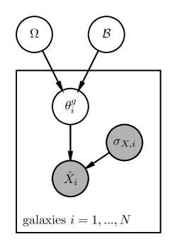
Figure 2: Graphical representation of our hierarchical approach that illustrate the relationship among the parameters of our model. White circles are inferred random variables and dark shaded circles are observed quantities. The physical properties of galaxies, $\theta^{g}_{i}$, are determined from the cosmological and hydrodynamical parameters $\Omega$ and $\mathcal{B}$ through CAMELS-TNG. Then the noisy optical photometry, $\hat{X}_{i}$, is derived from $\theta^{g}_{i}$ using SPS and our noise model.

4 Methods

4.1 Hierarchical Bayesian Population Inference

Our goal is to infer the posterior of cosmological parameters $\Omega=\{\Omega_{m},\sigma_{8}\}$ and baryonic feedback parameters $\mathcal{B}$ from the observed photometry of galaxies in the NSA catalog, $\{\textbf{{X}}_{i}\}$: $p(\Omega,\mathcal{B}\,|\,\{{\textbf{{X}}_{i}}\})$. ${\textbf{{X}}_{i}}$ represents both the measured absolute magnitudes and uncertainties: $\{\hat{X}_{i},\hat{\sigma}_{X,i}\}$. With our forward model we can simulate noisy galaxy photometry from $\Omega$ and $\mathcal{B}$. Hence, the cosmological inference from photometry can be reformulated as a hierarchical population inference problem.

To illustrate this, we graphically represent our forward model in Figure 2. Circles and shaded circles represent random variables and observed quantities. $\theta_{i}^{g}$ represents the physical properties of galaxies (e.g. $M_{*}$, star-formation history), which are determined from $\Omega$ and $\mathcal{B}$ through CAMELS-TNG. Then the noisy photometry $\hat{X}_{i}$ is determined from $\theta_{i}^{g}$ through SPS and our noise model.

We can rewrite the posterior as:

$$p(\Omega,\mathcal{B}\,|\,\{{\textbf{{X}}_{i}}\})= ~{}\frac{p(\Omega,\mathcal{B})~{}p(\{{\textbf{{X}}_{i}}\}\,|\,\Omega,\mathcal{B})}{p(\{{\textbf{{X}}_{i}}\})}$$ (1)

$$= ~{}\frac{p(\Omega,\mathcal{B})}{p(\{\textbf{{X}}_{i}\})}\prod\limits_{i=1}^{N}p({\textbf{{X}}_{i}}\,|\,\Omega,\mathcal{B})$$ (2)

$$= ~{}\frac{p(\Omega,\mathcal{B})}{p(\{\textbf{{X}}_{i}\})}\prod\limits_{i=1}^{N}\frac{p(\textbf{{X}}_{i})\,p(\Omega,\mathcal{B}\,|\,{\textbf{{X}}_{i}})}{p(\Omega,\mathcal{B})}$$ (3)

$$= ~{}\frac{1}{p(\Omega,\mathcal{B})^{N-1}}\prod\limits_{i=1}^{N}p(\Omega,\mathcal{B}\,|\,{\textbf{{X}}_{i}})$$ (4)

Here, we assume that galaxies are i.i.d. Since we impose uniform priors, $p(\Omega,\mathcal{B})\propto 1$ (Sec. 3):

$$p(\Omega,\mathcal{B}\,|\,\{{\textbf{{X}}_{i}}\})\propto ~{}\prod\limits_{i=1}^{N}p(\Omega,\mathcal{B}\,|\,{\textbf{{X}}_{i}}).$$ (5)

Up to a constant, we can evaluate $p(\Omega,\mathcal{B}\,|\,\{{\textbf{{X}}_{i}}\})$ if we can accurately estimate $p(\Omega,\mathcal{B}\,|\,{\textbf{{X}}_{i}})$, the posterior for any single galaxy under uniform priors.

4.2 Neural Density Estimation

One way to accurately estimate $p(\Omega,\mathcal{B}\,|\,{\textbf{{X}}_{i}})$ is by applying neural density estimation (NDE) to the CAMELS-TNG, which provides a training dataset of 100,000 parameter-photometry pairs: $\{(\Omega,\mathcal{B},{\textbf{{X}}_{i}})\}$. With NDE, we can use this data to train a neural network $q$ with parameters $\phi$ to estimate $q_{\phi}(\Omega,\mathcal{B}\,|\,{\textbf{{X}}_{i}})\approx p(\Omega,\mathcal{B}\,|\,{\textbf{{X}}_{i}})$. This type of simulation-based inference using NDE has been applied to a broad range of astronomical applications (e.g.  Wong et al., 2020; Dax et al., 2021; Zhang et al., 2021; Hahn et al., 2022a).

In this work, our NDE is based on “normalizing flow” models (Tabak & Vanden-Eijnden, 2010; Tabak & Turner, 2013; Jimenez Rezende & Mohamed, 2015), which use neural networks to learn a flexible and bijective transformation, $f$, that maps a complex target distribution to a simple base distribution that is fast to evaluate. $f$ is defined to be invertible and have a tractable Jacobian, so that the target distribution can be evaluated with change of variables. In our case, the target distribution is $p(\Omega,\mathcal{B}\,|\,{\textbf{{X}}_{i}})$, and we set the base distribution to be a multivariate Gaussian. Among different flow architectures, we use Masked Autoregressive Flow (MAF; Papamakarios et al., 2017) models implemented in the $\mathtt{sbi}$ Python package (Greenberg et al., 2019; Tejero-Cantero et al., 2020).

During training, we want to determine $q_{\phi}$ that best approximates $p(\Omega,\mathcal{B}\,|\,{\textbf{{X}}_{i}})$. We reformulate this into an optimization problem of determining $\phi$ that minimizes the KL divergence between $p(\Omega,\mathcal{B},{\textbf{{X}}_{i}})=p(\Omega,\mathcal{B}\,|\,{\textbf{{X}}_{i}})p({\textbf{{X}}_{i}})$ and $q_{\phi}(\Omega,\mathcal{B}\,|\,{\textbf{{X}}_{i}})p({\textbf{{X}}_{i}})$. In practice, we split the CAMELS-TNG data into a training and validation set with a 90/10 split. Then, we maximize the total log-likelihood $\sum_{i}\log q_{\phi}(\Omega,\mathcal{B}\,|\,{\textbf{{X}}_{i}})$ over the training set, which is equivalent to minimizing the KL divergence. To prevent overfitting, we evaluate the total log-likelihood on the validation data at every training epoch and stop the training when the validation log-likelihood fails to increase after 20 epochs.

We train a large number of flows ($\sim$2000) with architectures determined by the Akiba et al. (2019) hyperparameter optimization. We allow the numbers of blocks, transforms, and hidden neurons as well as the dropout probability and the learning rate to vary. Then, we construct our final flow as an equally weighted ensemble of five flows with the lowest validation losses: $q_{\phi}(\Omega,\mathcal{B}\,|\,{\textbf{{X}}_{i}})=\sum_{j=1}^{5}q_{\phi,j}(\Omega,\mathcal{B}\,|\,{\textbf{{X}}_{i}})/5$. Ensembling flows with different initializations and architectures improves the overall robustness of our normalizing flow. In Appendix A, we extensively validate the accuracy of $q_{\phi}$, using Simulation-Based Calibration (Talts et al., 2020) and the Lemos et al. (2023) coverage test. Our combined flow is a near optimal estimate of the true posterior.

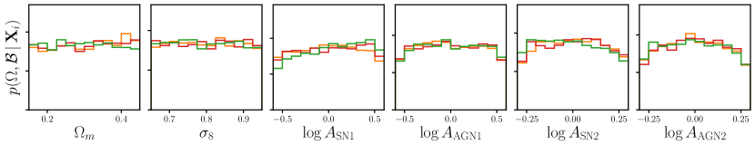
Figure 3: Estimated marginalized posteriors of the cosmological and hydrodynamical parameters ($\Omega$, $\mathcal{B}$) from photometry, $q_{\phi}(\Omega,\mathcal{B}\,|\,{\textbf{{X}}_{i}})$, for three arbitrarily selected NSA galaxies. The posteriors correspond to the galaxies marked in Figure 1. The photometry of a single galaxy contains limited cosmological information.

In Figure 3, we present $q_{\phi}(\Omega,\mathcal{B}\,|\,{\textbf{{X}}_{i}})$ for three arbitrarily selected NSA galaxies. We mark the colors and magnitudes of the selected galaxies in Figure 1 with crosses of the same color. The individual posteriors reveal that there is limited cosmological information in the photometry of a single galaxy. However, with Eq. 5 we can efficiently extract the cosmological information from entire galaxy surveys.

5 Results

With our trained NDE, $q_{\phi}(\Omega,\mathcal{B}\,|\,{\textbf{{X}}_{i}})$, we can now evaluate the posterior $p(\Omega,\mathcal{B}\,|\,\{\textbf{{X}}_{i}\})$ for multiple galaxies using Eq. 5. In Figure 4, we present $p(\Omega,\mathcal{B}\,|\,\{\textbf{{X}}_{i}\})$ for the 22,338 observed galaxies in our NSA sample. The contours mark the 68 and 95 percentiles of the distribution and we list the median and $\pm 1\sigma$ marginalized constraints on $\Omega_{m}$, $\sigma_{8}$, and $S_{8}=\sigma_{8}\sqrt{\Omega_{m}/0.3}$. The samples from $p(\Omega\,|\,\{\textbf{{X}}_{i}\})$ are derived using Markov Chain Monte Carlo (MCMC). We note that MCMC is necessary here since the individual posteriors $q_{\phi}(\Omega,\mathcal{B}\,|\,{\textbf{{X}}_{i}})$ are combined multiplicatively (Eq. 5), we cannot separately sample $q_{\phi}(\Omega,\mathcal{B}\,|\,{\textbf{{X}}_{i}})$ as this is equivalent to averaging the posteriors. We use the $\mathtt{emcee}$ sampler (Foreman-Mackey et al., 2013) with 1,000 walkers evaluated 100,000 iterations, discarding the first 10,000 iterations for burn in. This procedure requires ${\gg}10^{5}$ evaluations of the posterior per galaxy, which is computational prohibitive for standard sampling methods. However, NDE dramatically reduces this cost and make our approach computational feasible.

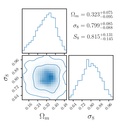
Figure 4: The posterior of $\Omega_{m}$ and $\sigma_{8}$ inferred from the observed photometry of 22,338 NSA galaxies. The contours mark the 68 and 95 percentiles. We place significant cosmological constraints from the photometry of galaxies alone.

Overall, we derive significant constraints on both $\Omega_{m}$ and $\sigma_{8}$: $\Omega_{m}=0.323^{+0.075}_{-0.095}$ and $\sigma_{8}=0.799^{+0.088}_{-0.085}$. We also derive significant constraints on the hydrodynamical parameters: $A_{\rm SN1}=0.996^{+0.573}_{-0.377}$, $A_{\rm AGN1}=0.987^{+0.603}_{-0.389}$, $A_{\rm SN2}=1.003^{+0.340}_{-0.287}$, and $A_{\rm AGN2}=1.017^{+0.396}_{-0.317}$. However, we do not include them in the figure for clarity. Our cosmological constraints demonstrate that although the photometry of a single galaxy does not contain a significant amount of cosmological information, we can place stringent cosmological constraints by combining the information from as little as 22,338 galaxies.

6 Discussion

A major caveat of our constraint is that our posterior assumes a galaxy formation and a SED models. This assumption is more clearly expressed if we rewrite

$$p(\Omega,\mathcal{B}\,|\,{\textbf{{X}}_{i}})\propto p(\Omega,\mathcal{B})\int p({\textbf{{X}}_{i}}\,|\,\theta^{g}_{i})\,p(\theta^{g}_{i}\,|\,\Omega,\mathcal{B})\,{\rm d}\theta^{g}_{i}.$$ (6)

In our case, $p(\theta^{g}_{i}\,|\,\Omega,\mathcal{B})$ is the TNG simulation and $p({\textbf{{X}}_{i}}\,|\,\theta^{g}_{i})$ is our forward model for photometry based on SED modeling.

TNG is a state-of-the-art hydrodynamical simulation. Yet it makes specific choices and assumptions, e.g. for its subgrid treatments for the formation and evolution of stellar populations, black hole growth, radiative cooling, stellar and black hole feedback, and magnetic fields (Pillepich et al., 2018; Nelson et al., 2018). Comparisons among hydrodynamical simulations (e.g. Hahn et al., 2019; Dickey et al., 2021), suggest that an alternative galaxy formation model may produce a significantly different $p(\theta^{g}_{i}\,|\,\Omega,\mathcal{B})$.

Similarly, the SED modeling, $p({\textbf{{X}}_{i}}\,|\,\theta^{g}_{i})$, includes a number of choices and assumptions. For instance, we use a dust model that assumes that dust is cospatial and uniformly mixed. Yet, recent studies suggest that the dust-star geometry can be significantly more complex and, thus, produce a wider range of attenuation curves (Narayanan et al., 2018; Hahn et al., 2021). The SED model also does not accurately model nebular emission lines, which may significantly impact the photometry of emission line galaxies. Furthermore, our SED model assumes a fixed Chabrier IMF. Observations, meanwhile, suggest that there may be significant variation (see Smith 2020 for a recent review).

A key advantage of our approach is that we can systematically choose specific galaxy populations that are most robust to variations in galaxy formation and SED models. For example, we can select galaxies that have consistent cosmological information, as predicted by multiple galaxy formation models. As Villaescusa-Navarro et al. (2022b) argue, the constraining power in galaxy properties on $\Omega_{m}$ comes from measuring the baryon fraction, $\Omega_{b}/\Omega_{m}$. This corresponds to measuring $M_{\rm tot}/M_{b}$ or $M_{\rm tot}/M_{*}/\epsilon_{*}$, where $\epsilon_{*}$ is the “star forming efficiency”. Galaxy formation models typically calibrate $M_{\rm tot}/M_{*}$ against constraints on the stellar-to-halo mass relation from observations (e.g. Mandelbaum et al., 2006; Behroozi et al., 2010; Moster et al., 2010; Leauthaud et al., 2012; Tinker et al., 2013; Zu & Mandelbaum, 2015; Gu et al., 2016, see also Wechsler & Tinker 2018 for a review). Hence, selecting galaxies that are robust to a change of the galaxy formation model boils down to selecting galaxies with consistent $\epsilon_{*}$ across models.

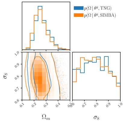
Figure 5: The cosmological information, $p(\Omega\,|\,\theta^{g})$, of a star-forming galaxy with $M_{*}\sim 10^{9.5}M_{\odot}$ and ${\rm SFR}=10^{-0.3}M_{\odot}/{\rm yr}$ from TNG (blue) and from SIMBA (orange). The contours mark the 68 and 95 percentiles. Specific galaxy populations, such as intermediate mass star-forming galaxies contain consistent cosmological information across different galaxy formation models.

One such population would be star-forming galaxies at intermediate $M_{*}$, whose relationship between gas and star formation are typically set by the empirical Kennicutt (1989) relation (e.g. Springel & Hernquist, 2003; Davé et al., 2016). To demonstrate this, in Figure 5, we compare the cosmological information content, $p(\Omega\,|\,\theta^{g}_{i})$, of a star-forming galaxy in TNG and a star-forming galaxy in SIMBA with similar galaxy properties: $M_{*}\sim 10^{9.5}M_{\odot}$ and ${\rm SFR}\sim 10^{-0.3}M_{\odot}/{\rm yr}$. The TNG and SIMBA galaxies contain highly consistent cosmological information.

Another possible way to identify galaxies that are robust to a change of the galaxy formation model is to find galaxies that lie well within the support a given galaxy formation model. Echeverri et al. (2023) showed that if you take galaxies from one galaxy formation model (e.g. TNG) and remove all the galaxies that are outliers of the model. The galaxies left have consistent cosmological information across multiple other galaxy formation models (e.g. SIMBA, Astrid, and Magneticum). Echeverri et al. (2023) identified the outlier galaxies using their physical properties, but this approach could be applied to observables (photometry) as well.

We can take a similar approach for the SED modeling assumptions by selecting galaxies without emission lines and with limited dust attenuation, e.g. as probed by infrared photometry. We can also identify galaxy populations with observationally well constrained IMFs or with little IMF variation (Myers et al., 2013; Smith et al., 2015). Alternatively, we can also allow the parameters of the SED model to vary and incorporate them in our hierarchical inference. This would broaden our constraints overall; however, Villaescusa-Navarro et al. (2023) promisingly find that the degradation in cosmological information of a single galaxy is limited even when allowing the IMF, and the vast majority of subgrid parameters in TNG, to vary.

Our posterior in Figure 4 places significant constraints on $\sigma_{8}$. In contrast, previous studies find limited constraining power on $\sigma_{8}$ from the properties of a single galaxy (Villaescusa-Navarro et al., 2022b; Echeverri et al., 2023). As Figure 5 illustrates, however, the constraining power on $\sigma_{8}$ is non-negligible. Furthermore, our constraint is consistent with the fact that $\sigma_{8}$ constraints tighten significantly when using the properties of multiple galaxies (Chawak et al., 2023). Population statistics, such as the stellar mass or luminosity function, are sensitive to $\sigma_{8}$. With multiple galaxies, we can effectively exploit this constraining power.

Lastly, we note that Eq. 5 does not include the selection function, $S$, applied to our NSA sample. In principle, we can include $S$ in our formulation and infer $p(\Omega,\mathcal{B}\,|\,\{\textbf{{X}}_{i}\},S)$. Given our uniform prior, $p(\Omega,\mathcal{B})\propto 1$, reformulating Eq. 5 with $S$ reduces to including an additional factor of $p(\Omega,\mathcal{B}\,|\,S)$. In this work, our selection is broadly set to remove any artifacts or objects with problematic photometry and to ensure that the NSA sample is within the support of our simulated galaxies. Including $p(\Omega,\mathcal{B}\,|\,S)$ has a negligible impact on our posterior.

7 Outlook

In this work, we selected $\sim$20,000 galaxies out of $\sim$120,000 in the NSA catalog, which provides photometry and spectroscopic redshifts. Upcoming spectroscopic surveys such as the Dark Energy Spectroscopic Survey (DESI; DESI Collab. et al., 2022) Bright Galaxy Survey (BGS; Hahn et al., 2022b) will observe orders of magnitude larger galaxy samples. With the tens of millions of galaxies that they will observe, these surveys will create enormous sample sizes even when we restrict the galaxy populations to those that are easy to model. This work can be directly extended to the observations from these surveys and leverage their unprecedented statistical power.

We can also extend this work to upcoming photometric surveys, namely the Vera C. Rubin Observatory (Ivezić et al., 2019). In this work, we relied on spectroscopic redshifts to limit our observation sample to a narrow redshift range. However, we can instead include $z$ as an additional parameter in $\theta^{g}$ and use forward modeled galaxies over a range of redshifts. Li et al. (2023) recently showed that the joint distribution of galaxy properties and redshift for a galaxy population can be simultaneously inferred from their photometry. This suggests that even with photometric redshifts, we can leverage the information on galaxy properties to constrain cosmology. Furthermore, with photometric surveys, we would have access to the cosmological information in hundreds of millions of galaxies.

Beyond extending our work to larger samples, we can also include a wider range of observables. In this work, we focus on optical broadband photometry. However, other observable encode additional information on the physical properties of galaxies, and thus cosmological information. For instance, emission lines measured from galaxy spectra can characterize the star formation history and gas content of galaxies. In fact, even the continuum of galaxy spectra contain significant constraining power on galaxy properties over photometry (Hahn et al., 2023). Beyond optical, radio observations of neutral hydrogen can also constrain $V_{\rm max}$ from rotation curves (e.g. Rogstad & Shostak, 1971; Allen et al., 1973; de Blok et al., 2008). Incorporating these observables would increase the precision of individual posteriors and, thus, has the potential to produce precise cosmological constraints with relatively smaller galaxy samples. However, to leverage their constraining power, we would need a forward model that can accurately model them. So far, this remains a major obstacle.

Appendix A Validating the Neural Density Estimator

Our posterior (Eq. 5) requires an accurate estimate of the individual posterior from NDE: $p(\Omega,\mathcal{B}\,|\,{\textbf{{X}}_{i}})\approx q_{\phi}(\Omega,\mathcal{B}\,|\,{\textbf{{X}}_{i}})$ (Sec. 4.2). To validate $q_{\phi}$, we use 10% of the CAMELS-TNG data reserved for testing and two validation methods: (1) Simulation-Based Calibration (SBC) and (2) the “distance to random point” (DRP) coverage test.

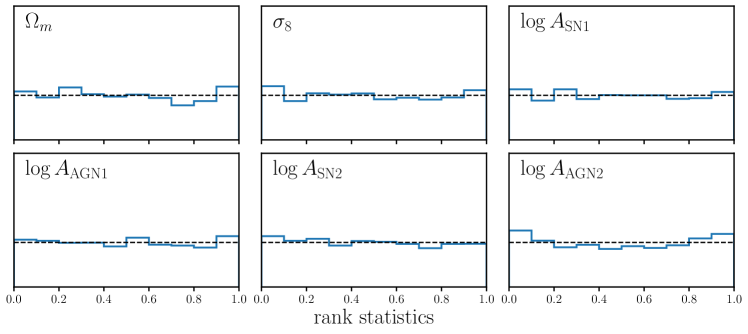
Figure 6: Simulation-based calibration plot of $q_{\phi}(\Omega,\mathcal{B}\,|\,{\textbf{{X}}_{i}})$ using 10% of the CAMELS-TNG data reserved for testing. The histogram in each panel represents the distribution of the rank statistic of the true value within the marginalized posterior (blue) for each parameter. The rank distribution is uniform for the true posterior (black dashed). The rank distribution of $q_{\phi}$ is nearly uniform for all $\Omega$ and $\mathcal{B}$ parameters. Therefore, it provides unbiased and accurate estimate of the true posterior.

Both are variations of the standard coverage test, where $q_{\phi}$ is applied to test samples not used for training. The posterior of each test sample is compared against the true parameter value, then the percentile score of the true parameter is calculated. Afterwards, cummulative distribution function (CDF) of the percentile is used to assess the accuracy of $q_{\phi}$. SBC is a modification of this standard coverage test that uses rank statistics rather than percentile score. It addresses the limitation that the CDFs only asymptotically approach the true values and that the discrete sampling of the posterior can cause artifacts in the CDFs. In Fig. 6, we present the SBC rank distributions of $q_{\phi}$ for $\Omega$ and $\mathcal{B}$ (blue). For the true posterior, rank distribution is uniform by construction (black dashed). The rank distributions are nearly uniform for all $\Omega$ and $\mathcal{B}$. Hence, we confirm that $q_{\phi}$ is in excellent agreement with the true posterior.

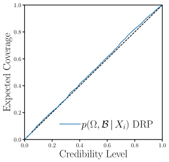
Figure 7: DRP coverage test validating the accuracy of our $q_{\phi}(\Omega,\mathcal{B}\,|\,{\textbf{{X}}_{i}})$ posterior estimate (blue). The DRP test is calculated using 10% of the CAMELS-TNG data reserved for testing. The black-dashed line represents an optimal estimate of the posterior. The DRP test demonstrates that $q_{\phi}$ provides a near optimal estimate of the true posterior.

As additional validation, we also use the DRP coverage test from Lemos et al. (2023). Instead of percentile scores or ranks, the DRP test assesses $q_{\phi}$ using samples drawn from $q_{\phi}$ for a test sample, the true parameter value of the test sample, and a random point in parameter space. It evalulates the distances between the $q_{\phi}$ samples and the random point. Then compares the distances to the distance between the true parameter value and the random point in order to derive an estimate of expected coverage probability. Lemos et al. (2023) prove that this approach is necessary and sufficient to show that a posterior estimator is optimal. In Fig. 7, we present the DRP coverage test of $q_{\phi}$ (blue). Based on the DRP test, $q_{\phi}$ provides a near optimal estimate of the true posterior (black-dashed).

color	16%	84%
$g-r$	0.313	0.722
$g-i$	0.510	1.086
$g-z$	0.670	1.385
$r-i$	0.190	0.368
$r-z$	0.345	0.673
$i-z$	0.142	0.316

Table 1: The 16 and 84 percentiles of the color distributions for the forward modeled CAMELS-TNG galaxies. We use these values as color cuts on the observed NSA sample (Section 2). This ensures that the observed sample lies within the support of our training data.

References

- Aihara et al. (2011) Aihara H., et al., 2011, The Astrophysical Journal Supplement Series, 193, 29
- Akiba et al. (2019) Akiba T., Sano S., Yanase T., Ohta T., Koyama M., 2019, Optuna: A Next-generation Hyperparameter Optimization Framework (arxiv:1907.10902), doi:10.48550/arXiv.1907.10902
- Allen et al. (1973) Allen R. J., Goss W. M., van Woerden H., 1973, A&A, 29, 447
- Aver et al. (2015) Aver E., Olive K. A., Skillman E. D., 2015, J. Cosmology Astropart. Phys, 2015, 011
- Behroozi et al. (2010) Behroozi P. S., Conroy C., Wechsler R. H., 2010, ApJ, 717, 379
- Bird et al. (2022) Bird S., Ni Y., Matteo T. D., Croft R., Feng Y., Chen N., 2022, Monthly Notices of the Royal Astronomical Society, 512, 3703
- Blanton & Roweis (2007) Blanton M. R., Roweis S., 2007, The Astronomical Journal, 133, 734
- Blanton et al. (2011) Blanton M. R., Kazin E., Muna D., Weaver B. A., Price-Whelan A., 2011, The Astronomical Journal, 142, 31
- Chabrier (2003) Chabrier G., 2003, Publications of the Astronomical Society of the Pacific, 115, 763
- Chawak et al. (2023) Chawak C., Villaescusa-Navarro F., Echeverri Rojas N., Ni Y., Hahn C., Angles-Alcazar D., 2023, arXiv e-prints, p. arXiv:2309.12048
- Conroy (2013) Conroy C., 2013, Annual Review of Astronomy and Astrophysics, 51, 393
- Conroy et al. (2009) Conroy C., Gunn J. E., White M., 2009, The Astrophysical Journal, 699, 486
- Cooke et al. (2018) Cooke R. J., Pettini M., Steidel C. C., 2018, ApJ, 855, 102
- DESI Collab. et al. (2022) DESI Collab. et al., 2022, Overview of the Instrumentation for the Dark Energy Spectroscopic Instrument (arxiv:2205.10939), doi:10.48550/arXiv.2205.10939
- Davé et al. (2016) Davé R., Thompson R., Hopkins P. F., 2016, MNRAS, 462, 3265
- Davé et al. (2019) Davé R., Anglés-Alcázar D., Narayanan D., Li Q., Rafieferantsoa M. H., Appleby S., 2019, Monthly Notices of the Royal Astronomical Society, 486, 2827
- Dax et al. (2021) Dax M., Green S. R., Gair J., Macke J. H., Buonanno A., Schölkopf B., 2021, Physical Review Letters, 127, 241103
- Dickey et al. (2021) Dickey C. M., et al., 2021, ApJ, 915, 53
- Echeverri et al. (2023) Echeverri N., et al., 2023, Cosmology with One Galaxy? – The ASTRID Model and Robustness (arxiv:2304.06084), doi:10.48550/arXiv.2304.06084
- Foreman-Mackey et al. (2013) Foreman-Mackey D., Hogg D. W., Lang D., Goodman J., 2013, Publications of the Astronomical Society of the Pacific, 125, 306
- Greenberg et al. (2019) Greenberg D. S., Nonnenmacher M., Macke J. H., 2019, Automatic Posterior Transformation for Likelihood-Free Inference
- Gu et al. (2016) Gu M., Conroy C., Behroozi P., 2016, ApJ, 833, 2
- Hahn & Melchior (2022) Hahn C., Melchior P., 2022, Accelerated Bayesian SED Modeling Using Amortized Neural Posterior Estimation
- Hahn et al. (2019) Hahn C., et al., 2019, The Astrophysical Journal, 872, 160
- Hahn et al. (2021) Hahn C., et al., 2021, IQ Collaboratory III: The Empirical Dust Attenuation Framework – Taking Hydrodynamical Simulations with a Grain of Dust
- Hahn et al. (2022b) Hahn C., et al., 2022b, DESI Bright Galaxy Survey: Final Target Selection, Design, and Validation
- Hahn et al. (2022a) Hahn C., et al., 2022a, ${\rm S{\scriptsize IM}BIG}$: A Forward Modeling Approach To Analyzing Galaxy Clustering
- Hahn et al. (2023) Hahn C., et al., 2023, ApJ, 945, 16
- Ivezić et al. (2019) Ivezić Ž., et al., 2019, ApJ, 873, 111
- Jeffrey & Wandelt (2020) Jeffrey N., Wandelt B. D., 2020, arXiv:2011.05991 [astro-ph, stat]
- Jimenez Rezende & Mohamed (2015) Jimenez Rezende D., Mohamed S., 2015, arXiv e-prints, p. arXiv:1505.05770
- Kennicutt (1989) Kennicutt Robert C. J., 1989, ApJ, 344, 685
- Leauthaud et al. (2012) Leauthaud A., et al., 2012, ApJ, 744, 159
- Lemos et al. (2023) Lemos P., Coogan A., Hezaveh Y., Perreault-Levasseur L., 2023, Sampling-Based Accuracy Testing of Posterior Estimators for General Inference, https://arxiv.org/abs/2302.03026v1
- Li et al. (2023) Li J., Melchior P., Hahn C., Huang S., 2023, arXiv e-prints, p. arXiv:2309.16958
- Mandelbaum et al. (2006) Mandelbaum R., Seljak U., Kauffmann G., Hirata C. M., Brinkmann J., 2006, MNRAS, 368, 715
- Moster et al. (2010) Moster B. P., Somerville R. S., Maulbetsch C., van den Bosch F. C., Macciò A. V., Naab T., Oser L., 2010, ApJ, 710, 903
- Myers et al. (2013) Myers A. T., McKee C. F., Cunningham A. J., Klein R. I., Krumholz M. R., 2013, The Astrophysical Journal, 766, 97
- Narayanan et al. (2018) Narayanan D., Conroy C., Davé R., Johnson B. D., Popping G., 2018, The Astrophysical Journal, 869, 70
- Nelson et al. (2018) Nelson D., et al., 2018, Monthly Notices of the Royal Astronomical Society, 475, 624
- Ni et al. (2022) Ni Y., et al., 2022, Monthly Notices of the Royal Astronomical Society, 513, 670
- Papamakarios et al. (2017) Papamakarios G., Pavlakou T., Murray I., 2017, arXiv e-prints, 1705, arXiv:1705.07057
- Pillepich et al. (2018) Pillepich A., et al., 2018, Monthly Notices of the Royal Astronomical Society, 473, 4077
- Rogstad & Shostak (1971) Rogstad D. H., Shostak G. S., 1971, A&A, 13, 99
- Schöneberg et al. (2019) Schöneberg N., Lesgourgues J., Hooper D. C., 2019, J. Cosmology Astropart. Phys, 2019, 029
- Smith (2020) Smith R. J., 2020, ARA&A, 58, 577
- Smith et al. (2015) Smith R. J., Lucey J. R., Conroy C., 2015, Monthly Notices of the Royal Astronomical Society, 449, 3441
- Springel & Hernquist (2003) Springel V., Hernquist L., 2003, MNRAS, 339, 289
- Tabak & Turner (2013) Tabak E. G., Turner C. V., 2013, Communications on Pure and Applied Mathematics, 66, 145
- Tabak & Vanden-Eijnden (2010) Tabak E. G., Vanden-Eijnden E., 2010, Communications in Mathematical Sciences, 8, 217
- Talts et al. (2020) Talts S., Betancourt M., Simpson D., Vehtari A., Gelman A., 2020, arXiv:1804.06788 [stat]
- Tejero-Cantero et al. (2020) Tejero-Cantero A., Boelts J., Deistler M., Lueckmann J.-M., Durkan C., Gonçalves P. J., Greenberg D. S., Macke J. H., 2020, Journal of Open Source Software, 5, 2505
- Tinker et al. (2013) Tinker J. L., Leauthaud A., Bundy K., George M. R., Behroozi P., Massey R., Rhodes J., Wechsler R. H., 2013, ApJ, 778, 93
- Villaescusa-Navarro et al. (2021) Villaescusa-Navarro F., et al., 2021, The Astrophysical Journal, 915, 71
- Villaescusa-Navarro et al. (2022a) Villaescusa-Navarro F., et al., 2022a, arXiv:2201.01300 [astro-ph]
- Villaescusa-Navarro et al. (2022b) Villaescusa-Navarro F., et al., 2022b, The Astrophysical Journal, 929, 132
- Villaescusa-Navarro et al. (2023) Villaescusa-Navarro F., sapace filler al. 2023, in preparation
- Wechsler & Tinker (2018) Wechsler R. H., Tinker J. L., 2018, ARA&A, 56, 435
- Weinberger et al. (2018) Weinberger R., et al., 2018, Monthly Notices of the Royal Astronomical Society, 479, 4056
- White et al. (1993) White S. D. M., Navarro J. F., Evrard A. E., Frenk C. S., 1993, Nature, 366, 429
- Wong et al. (2020) Wong K. W. K., Contardo G., Ho S., 2020, Physical Review D, 101, 123005
- Zhang et al. (2021) Zhang K., Bloom J. S., Gaudi B. S., Lanusse F., Lam C., Lu J. R., 2021, The Astronomical Journal, 161, 262
- Zu & Mandelbaum (2015) Zu Y., Mandelbaum R., 2015, MNRAS, 454, 1161
- de Blok et al. (2008) de Blok W. J. G., Walter F., Brinks E., Trachternach C., Oh S. H., Kennicutt R. C. J., 2008, AJ, 136, 2648