4D Gaussian Splatting for Real-Time Dynamic Scene Rendering

Abstract

Representing and rendering dynamic scenes has been an important but challenging task. Especially, to accurately model complex motions, high efficiency is usually hard to guarantee. To achieve real-time dynamic scene rendering while also enjoying high training and storage efficiency, we propose 4D Gaussian Splatting (4D-GS) as a holistic representation for dynamic scenes rather than applying 3D-GS for each individual frame. In 4D-GS, a novel explicit representation containing both 3D Gaussians and 4D neural voxels is proposed. A decomposed neural voxel encoding algorithm inspired by HexPlane is proposed to efficiently build Gaussian features from 4D neural voxels and then a lightweight MLP is applied to predict Gaussian deformations at novel timestamps. Our 4D-GS method achieves real-time rendering under high resolutions, 82 FPS at an 800$\times$800 resolution on an RTX 3090 GPU while maintaining comparable or better quality than previous state-of-the-art methods. More demos and code are available at https://guanjunwu.github.io/4dgs/.

^‡The rendering speed not only depends on the image resolution but also the number of 3D Gaussians and the scale of deformation fields which are determined by the complexity of the scene.

1 Introduction

Novel view synthesis (NVS) stands as a critical task in the domain of 3D vision and plays a vital role in many applications, e.g. VR, AR, and movie production. NVS aims at rendering images from any desired viewpoint or timestamp of a scene, usually requiring modeling the scene accurately from several 2D images. Dynamic scenes are quite common in real scenarios, rendering which is important but challenging as complex motions need to be modeled with both spatially and temporally sparse input.

NeRF [22] has achieved great success in synthesizing novel view images by representing scenes with implicit functions. The volume rendering techniques [5] are introduced to connect 2D images and 3D scenes. However, the original NeRF method bears big training and rendering costs. Though some NeRF variants [36, 6, 4, 8, 34, 7, 23] reduce the training time from days to minutes, the rendering process still bears a non-negligible latency.

Recent 3D Gaussian Splatting (3D-GS) [14] significantly boosts the rendering speed to a real-time level by representing the scene as 3D Gaussians. The cumbersome volume rendering in the original NeRF is replaced with efficient differentiable splatting [46], which directly projects 3D Gaussian points onto the 2D plane. 3D-GS not only enjoys real-time rendering speed but also represents the scene more explicitly, making it easier to manipulate the scene representation.

However, 3D-GS focuses on the static scenes. Extending it to dynamic scenes as a 4D representation is a reasonable, important but difficult topic. The key challenge lies in modeling complicated point motions from sparse input. 3D-GS holds a natural geometry prior by representing scenes with point-like Gaussians. One direct and effective extension approach is to construct 3D Gaussians at each timestamp [21] but the storage/memory cost will multiply especially for long input sequences. Our goal is to construct a compact representation while maintaining both training and rendering efficiency, i.e. 4D Gaussian Splatting (4D-GS). To this end, we propose to represent Gaussian motions and shape changes by an efficient Gaussian deformation field network, containing a temporal-spatial structure encoder and an extremely tiny multi-head Gaussian deformation decoder. Only one set of canonical 3D Gaussians is maintained. For each timestamp, the canonical 3D Gaussians will be transformed by the Gaussian deformation field into new positions with new shapes. The transformation process represents both the Gaussian motion and deformation. Note that different from modeling motions of each Gaussian separately [21, 44], the spatial-temporal structure encoder can connect different adjacent 3D Gaussians to predict more accurate motions and shape deformation. Then the deformed 3D Gaussians can be directly splatted for rendering the according-timestamp image. Our contributions can be summarized as follows.

• An efficient 4D Gaussian splatting framework with an efficient Gaussian deformation field is proposed by modeling both Gaussian motion and Gaussian shape changes across time.

• A multi-resolution encoding method is proposed to connect the nearby 3D Gaussians and build rich 3D Gaussian features by an efficient spatial-temporal structure encoder.

• 4D-GS achieves real-time rendering on dynamic scenes, up to 82 FPS at a resolution of 800$\times$800 for synthetic datasets and 30 FPS at a resolution of 1352$\times$1014 in real datasets, while maintaining comparable or superior performance than previous state-of-the-art (SOTA) methods and shows potential for editing and tracking in 4D scenes.

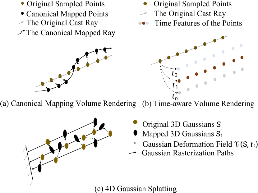
Figure 2: Illustration of different dynamic scene rendering methods. (a) Points are sampled in the casted ray during volume rendering. The point deformation fields proposed in [28, 6] map the points into a canonical space. (b) Time-aware volume rendering computes the features of each point directly and does not change the rendering path. (c) The Gaussian deformation field converts original 3D Gaussians into another group of 3D Gaussians with a certain timestamp.

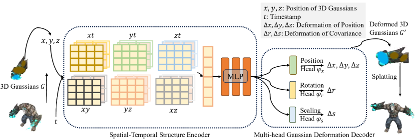
Figure 3: The overall pipeline of our model. Given a group of 3D Gaussians $\mathcal{G}$, we extract the center coordinate of each 3D Gaussian $\mathcal{X}$ and timestamp $t$ to compute the voxel feature by querying multi-resolution voxel planes. Then a tiny multi-head Gaussian deformation decoder is used to decode the feature and get the deformed 3D Gaussians $\mathcal{G}^{\prime}$ at timestamp $t$. The deformed Gaussians are then splatted to the rendered image.

2 Related Works

In this section, we simply review the difference of dynamic NeRFs in Sec. 2.1, then discuss the point clouds-based neural rendering algorithm in Sec. 2.2.

2.1 Dynamic Neural Rendering

[22, 3, 48] demonstrate that implicit radiance fields can effectively learn scene representations and synthesize high-quality novel views. [28, 24, 25] have challenged the static hypothesis, expanding the boundary of novel view synthesis for dynamic scenes. Additionally, [6] proposes to use an explicit voxel grid to model temporal information, accelerating the learning time for dynamic scenes to half an hour and applied in [45, 20, 12]. The proposed canonical mapping neural rendering methods are shown in Fig. 2 (a).  [17, 4, 8, 34, 37] represent further advancements in faster dynamic scene learning by adopting decomposed neural voxels. They treat sampled points in each timestamp individually as shown in Fig. 2 (b). [40, 11, 27, 42, 18, 38] are efficient methods to handle multi-view setups. The aforementioned methods though achieve fast training speed, real-time rendering for dynamic scenes is still challenging, especially for monocular input. Our method aims at constructing a highly efficient training and rendering pipeline in Fig. 2 (c), while maintaining the quality, even for sparse inputs.

2.2 Neural Rendering with Point Clouds

Effectively representing 3D scenes remains a challenging topic. The community has explored various neural representations [22], e.g. meshes, point clouds [43], and hybrid approaches. Point-cloud-based methods [29, 30, 47, 19] initially target at 3D segmentation and classification. A representative approach for rendering presented in [43, 1] combines point cloud representations with volume rendering, achieving rapid convergence speed. [16, 15, 31] adopt differential point rendering technique for scene reconstructions. Additionally, 3D-GS [14] is notable for its pure explicit representation and differential point-based splatting methods, enabling real-time rendering of novel views. Dynamic3DGS [21] models dynamic scenes by tracking the position and variance of each 3D Gaussian at each timestamp $t_{i}$. An explicit table is utilized to store information about each 3D Gaussian at every timestamp, leading to a linear memory consumption increase, denoted as $O(t\mathcal{N})$, in which $\mathcal{N}$ is num of 3D Gaussians. For long-term scene reconstruction, the storage cost will become non-negligible. The memory complexity of our approach only depends on the number of 3D Gaussians and parameters of Gaussians deformation fields network $\mathcal{F}$, which is denoted as $O(\mathcal{N}+\mathcal{F})$. [44] adds a marginal temporal Gaussian distribution into the origin 3D Gaussians, which uplift 3D Gaussians into 4D. However, it may cause each 3D Gaussian to only focus on their local temporal space. Our approach also models 3D Gaussian motions but with a compact network, resulting in highly efficient training efficiency and real-time rendering.

3 Preliminary

In this section, we simply review the representation and rendering process of 3D-GS [14] in Sec. 3.1 and the formula of dynamic NeRFs in Sec. 3.2.

3.1 3D Gaussian Splatting

3D Gaussians [14] is an explicit 3D scene representation in the form of point clouds. Each 3D Gaussian is characterized by a covariance matrix $\Sigma$ and a center point $\mathcal{X}$, which is referred to as the mean value of the Gaussian:

$$G(X)=e^{-\frac{1}{2}\mathcal{X}^{T}\Sigma^{-1}\mathcal{X}}.$$ (1)

For differentiable optimization, the covariance matrix $\Sigma$ can be decomposed into a scaling matrix $\mathbf{S}$ and a rotation matrix $\mathbf{R}$:

$$\Sigma=\mathbf{R}\mathbf{S}\mathbf{S}^{T}\mathbf{R}^{T}.$$ (2)

When rendering novel views, differential splatting [46] is employed for the 3D Gaussians within the camera planes. As introduced by [50], using a viewing transform matrix $W$ and the Jacobian matrix $J$ of the affine approximation of the projective transformation, the covariance matrix $\Sigma^{\prime}$ in camera coordinates can be computed as

$$\Sigma^{\prime}=JW\Sigma W^{T}J^{T}.$$ (3)

In summary, each 3D Gaussian is characterized by the following attributes: position $\mathcal{X}\in\mathbb{R}^{3}$, color defined by spherical harmonic (SH) coefficients $\mathcal{C}\in\mathbb{R}^{k}$ (where $k$ represents nums of SH functions), opacity $\alpha\in\mathbb{R}$, rotation factor $r\in\mathbb{R}^{4}$, and scaling factor $s\in\mathbb{R}^{3}$. Specifically, for each pixel, the color and opacity of all the Gaussians are computed using the Gaussian’s representation Eq. 1. The blending of $N$ ordered points that overlap the pixel is given by the formula:

$$C=\sum_{i\in N}c_{i}\alpha_{i}\prod_{j=1}^{i-1}(1-\alpha_{i}).$$ (4)

Here, $c_{i}$, $\alpha_{i}$ represents the density and color of this point computed by a 3D Gaussian $G$ with covariance $\Sigma$ multiplied by an optimizable per-point opacity and SH color coefficients.

3.2 Dynamic NeRFs with Deformation Fields

All the dynamic NeRF algorithms can be formulated as:

$$c,\sigma=\mathcal{M}(\mathbf{x},t),$$ (5)

where $\mathcal{M}$ is a mapping that maps 6D space $(\mathbf{x},d,t)$ to 4D space $(c,\sigma)$. Dynamic NeRFs mainly follow two paths: canonical-mapping volume rendering [28, 24, 25, 6, 20] and time-aware volume rendering [9, 17, 4, 8, 34]. In this section, we mainly give a brief review of the former.

As is shown in Fig. 2 (a), the canonical-mapping volume rendering transforms each sampled point into a canonical space by a deformation network $\phi_{t}:(\mathbf{x},t)\rightarrow\Delta\mathbf{x}$. Then a canonical network $\phi_{x}$ is introduced to regress volume density and view-dependent RGB color from each ray. The formula for rendering can be expressed as:

$$c,\sigma=\text{NeRF}(\mathbf{x}+\Delta\mathbf{x}),$$ (6)

where ‘NeRF’ stands for vanilla NeRF pipeline.

However, our 4D Gaussian splatting framework presents a novel rendering technique. We transform 3D Gaussians using a Gaussian deformation field network $\mathcal{F}$ at the time $t$ directly and differential splatting [14] is followed.

4 Method

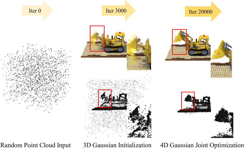
Figure 4: Illustration of the optimization process. With static 3D Gaussian initialization, our model can learn high-quality 3D Gaussians of the motion part.

Sec. 4.1 introduces the overall 4D Gaussian Splatting framework. Then, the Gaussian deformation field is proposed in Sec. 4.2. Finally, we describe the optimization process in Sec. 4.3.

4.1 4D Gaussian Splatting Framework

As shown in Fig. 3, given a view matrix $M=[R,T]$, timestamp $t$, our 4D Gaussian splatting framework includes 3D Gaussians $\mathcal{G}$ and Gaussian deformation field network $\mathcal{F}$. Then a novel-view image $\hat{I}$ is rendered by differential splatting [46] $\mathcal{S}$ following $\hat{I}=\mathcal{S}(M,\mathcal{G}^{\prime})$, where $\mathcal{G}^{\prime}=\Delta\mathcal{G}+\mathcal{G}$.

Specifically, the deformation of 3D Gaussians $\Delta\mathcal{G}$ is introduced by the Gaussian deformation field network $\Delta\mathcal{G}=\mathcal{F}(\mathcal{G},t)$, in which the spatial-temporal structure encoder $\mathcal{H}$ can encode both the temporal and spatial features of 3D Gaussians $f_{d}=\mathcal{H}(\mathcal{G},t)$, and the multi-head Gaussian deformation decoder $\mathcal{D}$ can decode the features and predict each 3D Gaussian’s deformation $\Delta\mathcal{G}=\mathcal{D}(f)$, then the deformed 3D Gaussians $\mathcal{G}^{\prime}$ can be introduced.

The rendering process of our 4D Gaussian Splatting is depicted in Fig. 2 (c). Our 4D Gaussian splatting converts the original 3D Gaussians $\mathcal{G}$ into another group of 3D Gaussians $\mathcal{G}^{\prime}$ given a timestamp $t$, maintaining the effectiveness of the differential splatting as referred in [46].

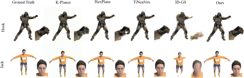
Figure 5: Visualization of synthesized datasets compared with other models [4, 8, 6, 14, 12, 37]. The rendering results of [8] are displayed with a default green background. We have adopted their rendering settings.

4.2 Gaussian Deformation Field Network

The network to learn the Gaussian deformation field includes an efficient spatial-temporal structure encoder $\mathcal{H}$ and a Gaussian deformation decoder $\mathcal{D}$ for predicting the deformation of each 3D Gaussian.

Spatial-Temporal Structure Encoder.

Nearby 3D Gaussians always share similar spatial and temporal information. To model 3D Gaussians’ features effectively, we introduce an efficient spatial-temporal structure encoder $\mathcal{H}$ including a multi-resolution HexPlane $R(i,j)$ and a tiny MLP $\phi_{d}$ inspired by  [6, 4, 8, 34]. While the vanilla 4D neural voxel is memory-consuming, we adopt a 4D K-Planes [8] module to decompose the 4D neural voxel into 6 planes. All 3D Gaussians in a certain area can be contained in the bounding plane voxels and Gaussian’s deformation can also be encoded in nearby temporal voxels.

Specifically, the spatial-temporal structure encoder $\mathcal{H}$ contains 6 multi-resolution plane modules $R_{l}(i,j)$ and a tiny MLP $\phi_{d}$, i.e. $\mathcal{H}(\mathcal{G},t)=\{R_{l}(i,j),\phi_{d}|(i,j)\in\{(x,y),(x,z),(y,z),(x,t),(y,t),(z,t)\},l\in\{1,2\}\}$. The position $\mathcal{X}=(x,y,z)$ is the mean value of 3D Gaussians $\mathcal{G}$. Each voxel module is defined by $R(i,j)\in\mathbb{R}^{h\times lN_{i}\times lN_{j}}$, where $h$ stands for the hidden dim of features, $N$ denotes the basic resolution of voxel grid and $l$ equals to the upsampling scale. This entails encoding information of the 3D Gaussians within the 6 2D voxel planes while considering temporal information. The formula for computing separate voxel features is as follows:

$$f_{h} =\bigcup_{l}\prod\text{interp}(R_{l}(i,j)),$$ (7)

$$(i,j) \in\{(x,y),(x,z),(y,z),(x,t),(y,t),(z,t)\}.$$

$f_{h}\in\mathbb{R}^{h*l}$ is the feature of neural voxels. ‘interp’ denotes the bilinear interpolation for querying the voxel features located at 4 vertices of the grid. The discussion of the production process is similar to [8]. Then a tiny MLP $\phi_{d}$ merges all the features by $f_{d}=\phi_{d}(f_{h})$.

Multi-head Gaussian Deformation Decoder.

When all the features of 3D Gaussians are encoded, we can compute any desired variable with a multi-head Gaussian deformation decoder $\mathcal{D}=\{\phi_{x},\phi_{r},\phi_{s}\}$. Separate MLPs are employed to compute the deformation of position $\Delta\mathcal{X}=\phi_{x}(f_{d})$, rotation $\Delta r=\phi_{r}(f_{d})$, and scaling $\Delta s=\phi_{s}(f_{d})$. Then, the deformed feature $(\mathcal{X}^{\prime},r^{\prime},s^{\prime})$ can be addressed as:

$$(\mathcal{X}^{\prime},r^{\prime},s^{\prime})=(\mathcal{X}+\Delta\mathcal{X},r+\Delta r,s+\Delta s).$$ (8)

Finally, we obtain the deformed 3D Gaussians $\mathcal{G}^{\prime}=\{\mathcal{X}^{\prime},s^{\prime},r^{\prime},\sigma,\mathcal{C}\}$.

4.3 Optimization

3D Gaussian Initialization.

[14] shows that 3D Gaussians can be well-trained with structure from motion (SfM) [32] points initialization. Similarly, 4D Gaussians should also be fine-tuned in proper 3D Gaussian initialization. We optimize 3D Gaussians at initial 3000 iterations for warm-up and then render images with 3D Gaussians $\hat{I}=\mathcal{S}(M,\mathcal{G})$ instead of 4D Gaussians $\hat{I}=\mathcal{S}(M,\mathcal{G}^{\prime})$. The illustration of the optimization process is shown in Fig. 4.

Loss Function.

Similar to other reconstruction methods [14, 28, 6], we use the L1 color loss to supervise the training process. A grid-based total-variational loss [36, 6, 4, 8] $\mathcal{L}_{tv}$ is also applied.

$$\mathcal{L}=\hat{I}-I+\mathcal{L}_{tv}.$$ (9)

Figure 6: Visualization of the HyperNeRF [25] datasets compared with other methods [14, 25, 6, 12]. ‘GT’ stands for ground truth images.

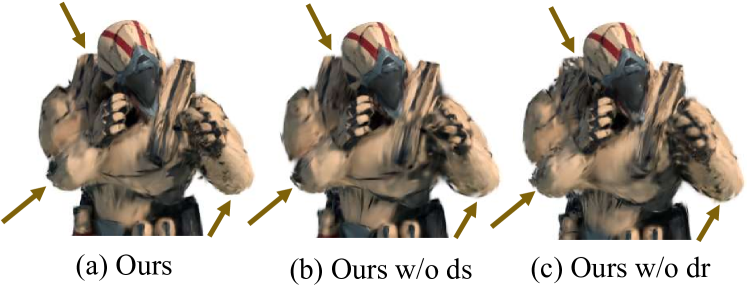
Figure 7: Ablation Study of the rotation and scaling decoder. ‘ds’ denotes as $\phi_{s}$ and, ‘’dr’ stands for $\phi_{r}$.

Table 1: Quantitative results on the synthesis dataset. The best and the second best results are denoted by pink and yellow. The rendering resolution is set to 800$\times$800. “Time” in the table stands for training times.

Model	PSNR(dB)↑	SSIM↑	LPIPS↓	Time↓	FPS ↑	Storage (MB)↓
TiNeuVox-B [6]	32.67	0.97	0.04	28 mins	1.5	48
KPlanes [8]	31.61	0.97	-	52 mins	0.97	418
HexPlane-Slim [4]	31.04	0.97	0.04	11m 30s	2.5	38
3D-GS [14]	23.19	0.93	0.08	10 mins	170	10
FFDNeRF [12]	32.68	0.97	0.04	-	$<$ 1	440
MSTH [37]	31.34	0.98	0.02	6 mins	-	-
Ours	34.05	0.98	0.02	20 mins	82	18

Table 2: Quantitative results on HyperNeRF’s [25] vrig dataset. Rendering resolution is set to 960$\times$540.

Model	PSNR(dB)↑	MS-SSIM↑	Times↓	FPS↑	Storage(MB)↓
Nerfies [24]	22.2	0.803	$\sim$ hours	$<$ 1	-
HyperNeRF [25]	22.4	0.814	32 hours	$<$ 1	-
TiNeuVox-B [6]	24.3	0.836	30 mins	1	48
3D-GS [14]	19.7	0.680	40 mins	55	52
FFDNeRF [12]	24.2	0.842	-	0.05	440
Ours	25.2	0.845	1 hour	34	61

Table 3: Quantitative results on the Neu3D’s [17] dataset, rendering resolution is set to 1352$\times$1014.

Model	PSNR(dB)↑	D-SSIM↓	LPIPS↓	Time ↓	FPS↑	Storage (MB)↓
NeRFPlayer [35]	30.69	0.034	0.111	6 hours	0.045	-
HyperReel [2]	31.10	0.036	0.096	9 hours	2.0	360
HexPlane-all* [4]	31.70	0.014	0.075	12 hours	0.2	250
KPlanes [8]	31.63	-	-	1.8 hours	0.3	309
Im4D [18]	32.58	-	0.208	28 mins	$\sim$5	93
MSTH [37]	32.37	0.015	0.056	20 mins	2(15‡)	135
Ours	31.15	0.016	0.049	40 mins	30	90

• *: The metrics of the model are tested without “coffee martini” and resolution is set to 1024$\times$768.

• ^‡: The FPS is tested with fixed-view rendering.

Table 4: Ablation studies on synthetic datasets using our proposed methods.

Model	PSNR(dB)↑	SSIM↑	LPIPS↓	Time↓	FPS↑	Storage (MB)↓
Ours w/o HexPlane $R_{l}(i,j)$	27.05	0.95	0.05	10 mins	140	12
Ours w/o initialization	31.91	0.97	0.03	19 mins	79	18
Ours w/o $\phi_{x}$	26.67	0.95	0.07	20 mins	82	17
Ours w/o $\phi_{r}$	33.08	0.98	0.03	20 mins	83	17
Ours w/o $\phi_{s}$	33.02	0.98	0.03	20 mins	82	17
Ours	34.05	0.98	0.02	20 mins	82	18

5 Experiment

In this section, we mainly introduce the hyperparameters and datasets of our settings in Sec. 5.1 and the results between different datasets will be compared with [6, 37, 38, 18, 2, 4, 8, 14, 35] in Sec. 5.2. Then, ablation studies are proposed to prove the effectiveness of our approaches in Sec. 5.3 and more discussion about 4D-GS in Sec. 5.4. Finally, we discuss the limitation of our proposed 4D-GS in Sec. 5.5.

5.1 Experimental Settings

Our implementation is primarily based on the PyTorch [26] framework and tested in a single RTX 3090 GPU, and we’ve fine-tuned our optimization parameters by the configuration outlined in the 3D-GS [14]. More hyperparameters will be shown in the appendix.

Synthetic Dataset.

We primarily assess the performance of our model using synthetic datasets, as introduced by D-NeRF [28]. These datasets are designed for monocular settings, although it’s worth noting that the camera poses for each timestamp are close to randomly generated. Each scene within these datasets contains dynamic frames, ranging from 50 to 200 in number.

Real-world Datasets.

We utilize datasets provided by HyperNeRF [25] and Neu3D’s [17] as benchmark datasets to evaluate the performance of our model in real-world scenarios. The Nerfies dataset is captured using one or two cameras, following straightforward camera motion, while the Neu3D’s dataset is captured using 15 to 20 static cameras, involving extended periods and intricate camera motions. We use the points computed by SfM [32] from the first frame of each video in Neu3D’s dataset and 200 frames randomly selected in HyperNeRF’s.

5.2 Results

We primarily assess our experimental results using various metrics, encompassing peak-signal-to-noise ratio (PSNR), perceptual quality measure LPIPS [49], structural similarity index (SSIM) [41] and its extensions including structural dissimilarity index measure (DSSIM), multiscale structural similarity index (MS-SSIM), FPS, training times and Storage.

To assess the quality of novel view synthesis, we conducted benchmarking against several state-of-the-art methods in the field, including  [6, 4, 8, 37, 14]. The results are summarized in Tab. 1. While current dynamic hybrid representations can produce high-quality results, they often come with the drawback of rendering speed. The lack of modeling dynamic motion part makes [14] fail to reconstruct dynamic scenes. In contrast, our method enjoys both the highest rendering quality within the synthesis dataset and exceptionally fast rendering speeds while keeping extremely low storage consumption and convergence time.

Additionally, the results obtained from real-world datasets are presented in Tab. 2 and Tab. 3. It becomes apparent that some NeRFs [35, 2, 4] suffer from slow convergence speed, and the other grid-based NeRF methods [6, 4, 37, 8] encounter difficulties when attempting to capture intricate object details. In stark contrast, our methods research comparable rendering quality, fast convergence, and excel in free-view rendering speed in indoor cases. Though [18] addresses the high quality in comparison to ours, the need for multi-cam setups makes it hard to model monocular scenes and other methods also limit free-view rendering speed and storage.

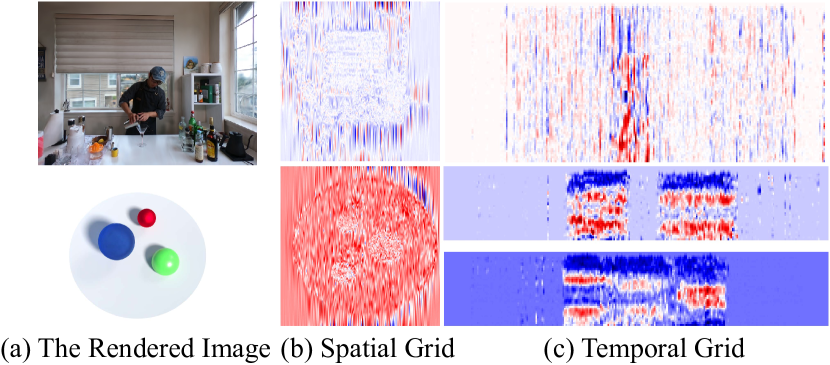
Figure 8: Visualization of HexPlane voxel grids. (a) are the rendered images. (b) are the parameters of spatial voxel grids, which implies the feature of 3D Gaussians are encoded in explicit grids. (c) are the temporal features of the grids, each column stands for spatial features in the timestamps.

5.3 Ablation Study

Spatial-Temporal Structure Encoder.

The explicit HexPlane encoder $R_{l}(i,j)$ possesses the capacity to retain 3D Gaussians’ spatial and temporal information, which can reduce storage consumption in comparison with purely explicit methods [21]. Discarding this module, we observe that using only a shallow MLP $\phi_{d}$ falls short in modeling complex deformations across various settings. Tab. 4 demonstrates that, while the model incurs minimal memory costs, it does come at the expense of rendering quality.

Gaussian Deformation Decoder.

Our proposed Gaussian deformation decoder $\mathcal{D}$ decodes the features from the spatial-temporal structure encoder $\mathcal{H}$. All the changes in 3D Gaussians can be explained by separate MLPs $\{\phi_{x},\phi_{r},\phi_{s}\}$. As is shown in Tab. 4, 4D Gaussians cannot fit dynamic scenes well without modeling 3D Gaussian motion. Meanwhile, the movement of human body joints is typically manifested as stretching and twisting of surface details in a macroscopic view. If one aims to accurately model these movements, the size and shape of 3D Gaussians should also be adjusted accordingly. Otherwise, there may be underfitting of details during excessive stretching, or an inability to correctly simulate the movement of objects at a microscopic level. Fig. 7 also demonstrates that shape deformation of 3D Gaussians is important in recovering details.

3D Gaussian Initialization.

In some cases without SfM [32] points initialization, training 4D-GS directly may cause difficulty in convergence. Optimizing 3D Gaussians for warm-up enjoys: (a) making some 3D Gaussians stay in the dynamic part, which releases the pressure of large deformation learning by 4D Gaussians as shown in Fig. 4. (b) learning proper 3D Gaussians $\mathcal{G}$ and suggesting deformation fields paying more attention to the dynamic part like Fig. 8(c). (c) avoiding numeric errors in optimizing the Gaussian deformation network $\mathcal{F}$ and keeping the training process stable. Tab. 4 also shows that if we train our model without the warm-up coarse stage, the rendering quality will suffer.

5.4 Discussions

Analysis of Multi-resolution HexPlane Gaussian Encoder.

The visualization of features in our multi-resolution HexPlane $R_{l}(i,j)$ is depicted in Fig. 8. As an explicit module, all the 3D Gaussians features can be easily optimized in individual voxel planes. It can be observed in Fig. 8 (b) that the voxel plane even shows a similar shape to the rendered image, such as edges. Meanwhile, the temporal features also stay in motion areas in the Fig. 8 (c). Such an explicit representation boosts the speed of training and rendering quality of our 4D Gaussians.

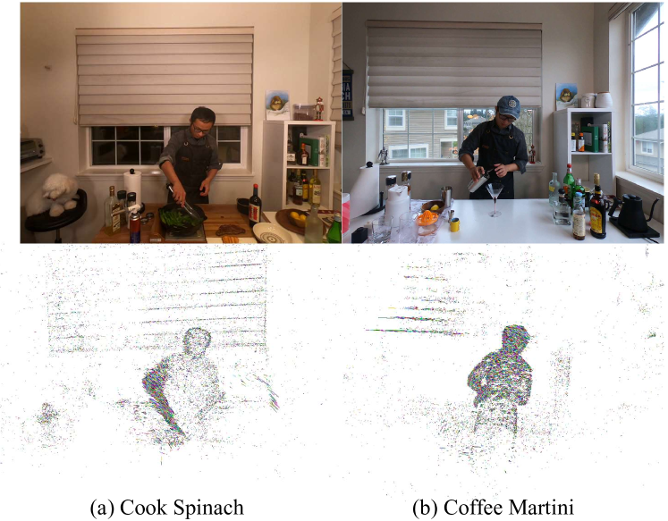
Figure 9: Visualization of tracking with 3D Gaussians. Each line in the figure of second rows stands for trajectories of 3D Gaussians

Tracking with 3D Gaussians.

Tracking in 3D is also a important task. [12] also shows tracking objects’ motion in 3D. Different from dynamic3DGS [21], our methods even can present tracking objects in monocular settings with pretty low storage i.e. 10MB in 3D Gaussians $\mathcal{G}$ and 8 MB in Gaussian deformation field network $\mathcal{F}$. Fig. 9 shows the 3D Gaussian’s deformation at certain timestamps.

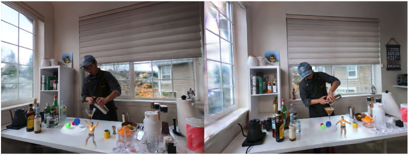
Figure 10: Visualization of composition with 4D Gaussians.

Composition with 4D Gaussians.

Similar to dynamic3DGS [21], our proposed methods can also propose composition with different 4D Gaussians in Fig. 10. Thanks to the explicit representation of 3D Gaussians, all the trained models can predict deformed 3D Gaussians in the same space following $\mathcal{G}^{\prime}=\{\mathcal{G}_{1}^{\prime},\mathcal{G}_{2}^{\prime},...,\mathcal{G}_{n}^{\prime}\}$ and differential rendering [46] can project all the point clouds into viewpoints by $\hat{I}=\mathcal{S}(M,\mathcal{G}^{\prime})$.

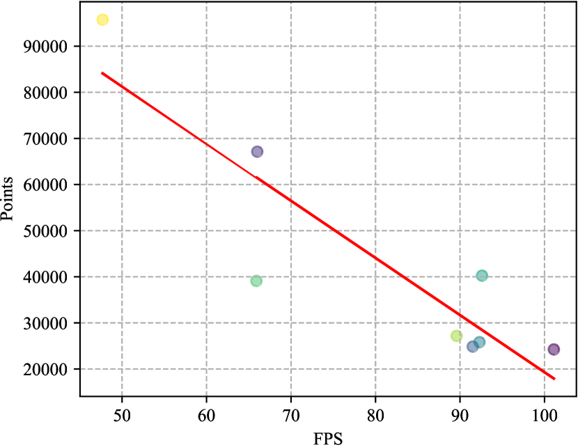
Figure 11: Visualization of the relationship between rendering speed and numbers of 3D Gaussians in the rendered screens. All the tests are finished in the synthesis dataset.

Analysis of Rendering Speed.

As is shown in Fig. 11, we also test the relationship between points in the rendered screen and rendering speed at the resolution of 800$\times$800. We found that if the rendered points are lower than 30000, the rendering speed can be up to 90. The config of Gaussian deformation fields are discussed in the appendix. To achieve render-time rendering speed, we should strike a balance among all the rendering resolutions, 4D Gaussians representation including numbers of 3D Gaussians, and the capacity of the Gaussian deformation field network and any other hardware constraints.

5.5 Limitations

Though 4D-GS can indeed attain rapid convergence and yield real-time rendering outcomes in many scenarios, there are a few key challenges to address. First, large motions, the absence of background points, and the unprecise camera pose cause the struggle of optimizing 4D Gaussians. What is more, it is still challenging to 4D-GS also cannot split the joint motion of static and dynamic Gaussiansparts under the monocular settings without any additional supervision. Finally, a more compact algorithm needs to be designed to handle urban-scale reconstruction due to the heavy querying of Gaussian deformation fields by huge numbers of 3D Gaussians.

6 Conclusion

This paper proposes 4D Gaussian splatting to achieve real-time dynamic scene rendering. An efficient deformation field network is constructed to accurately model Gaussian motions and shape deformations, where adjacent Gaussians are connected via a spatial-temporal structure encoder. Connections between Gaussians lead to more complete deformed geometry, effectively avoiding avulsion. Our 4D Gaussians can not only model dynamic scenes but also have the potential for 4D objective tracking and editing.

Table 5: Perscene results of HyperNeRF’s vrig datasets [25] by different models.

Method	3D Printer		Chicken		Broom		Banana
	PSNR	MS-SSIM	PSNR	MS-SSIM	PSNR	MS-SSIM	PSNR	MS-SSIM
Nerfies [24]	20.6	0.83	26.7	0.94	19.2	0.56	22.4	0.87
HyperNeRF [25]	20.0	0.59	26.9	0.94	19.3	0.59	23.3	0.90
TiNeuVox-B [6]	22.8	0.84	28.3	0.95	21.5	0.69	24.4	0.87
FFDNeRF [12]	22.8	0.84	28.0	0.94	21.9	0.71	24.3	0.86
3D-GS [14]	18.3	0.60	19.7	0.70	20.6	0.63	20.4	0.80
Ours	22.1	0.81	28.7	0.93	22.0	0.70	28.0	0.94

Table 6: Per-scene results of DyNeRF’s [17] datasets.

Method	Cut Beef		Cook Spinach		Sear Steak
	PSNR	SSIM	PSNR	SSIM	PSNR	SSIM
NeRFPlayer [35]	31.83	0.928	32.06	0.930	32.31	0.940
HexPlane [4]	32.71	0.985	31.86	0.983	32.09	0.986
KPlanes [8]	31.82	0.966	32.60	0.966	32.52	0.974
MixVoxels [38]	31.30	0.965	31.65	0.965	31.43	0.971
Ours	32.90	0.957	32.46	0.949	32.49	0.957
Method	Flame Steak		Flame Salmon		Coffee Martini
	PSNR	SSIM	PSNR	SSIM	PSNR	SSIM
NeRFPlayer [35]	27.36	0.867	26.14	0.849	32.05	0.938
HexPlane [4]	31.92	0.988	29.26	0.980	-	-
KPlanes [8]	32.39	0.970	30.44	0.953	29.99	0.953
MixVoxels [38]	31.21	0.970	29.92	0.945	29.36	0.946
Ours	32.51	0.954	29.20	0.917	27.34	0.905

Method	Bouncing Balls			Hellwarrior			Hook			Jumpingjacks
	PSNR	SSIM	LPIPS	PSNR	SSIM	LPIPS	PSNR	SSIM	LPIPS	PSNR	SSIM	LPIPS
3D-GS [14]	23.20	0.9591	0.0600	24.53	0.9336	0.0580	21.71	0.8876	0.1034	23.20	0.9591	0.0600
K-Planes[8]	40.05	0.9934	0.0322	24.58	0.9520	0.0824	28.12	0.9489	0.0662	31.11	0.9708	0.0468
HexPlane[4]	39.86	0.9915	0.0323	24.55	0.9443	0.0732	28.63	0.9572	0.0505	31.31	0.9729	0.0398
TiNeuVox[6]	40.23	0.9926	0.0416	27.10	0.9638	0.0768	28.63	0.9433	0.0636	33.49	0.9771	0.0408
Ours	40.62	0.9942	0.0155	28.71	0.9733	0.0369	32.73	0.9760	0.0272	35.42	0.9857	0.0128
Method	Lego			Mutant			Standup			Trex
	PSNR	SSIM	LPIPS	PSNR	SSIM	LPIPS	PSNR	SSIM	LPIPS	PSNR	SSIM	LPIPS
3D-GS [14]	23.06	0.9290	0.0642	20.64	0.9297	0.0828	21.91	0.9301	0.0785	21.93	0.9539	0.0487
K-Planes [8]	25.49	0.9483	0.0331	32.50	0.9713	0.0362	33.10	0.9793	0.0310	30.43	0.9737	0.0343
HexPlane [4]	25.10	0.9388	0.0437	33.67	0.9802	0.0261	34.40	0.9839	0.0204	30.67	0.9749	0.0273
TiNeuVox [6]	24.65	0.9063	0.0648	30.87	0.9607	0.0474	34.61	0.9797	0.0326	31.25	0.9666	0.0478
Ours	25.03	0.9376	0.0382	37.59	0.9880	0.0167	38.11	0.9898	0.0074	34.23	0.9850	0.0131

Table 7: Per-scene results of synthesis datasets.

Table 8: Ablation Study on $\phi_{\mathcal{C}}$ and $\phi_{\mathcal{\alpha}}$, comparing with TiNeuVox [6] in Americano of HyperNeRF [25]’s dataset.

Method	Americano
	PSNR	MS-SSIM
TiNeuVox-B [6]	28.4	0.96
Ours w/ $\phi_{\mathcal{C}}$,$\phi_{\mathcal{\alpha}}$	31.53	0.97
Ours	30.90	0.96

Appendix A Appendix

A.1 Introduction

In the supplementary material, we mainly introduce our hyperparameter settings of experiments in Sec. A.2. Then more ablation studies and discussions are conducted in Sec. A.3. Finally, we delve into the limitations of our proposed 4D-GS in Sec. A.4.

A.2 Hyperparameter Settings

Our hyperparameters mainly follow the settings of 3D-GS [14]. The basic resolution of our multi-resolution HexPlane module $R(i,j)$ is set to 64, which is upsampled by 2 and 4. The learning rate is set as $1.6\times 10^{-3}$, decayed to $1.6e-4$ at the end of training. The Gaussian deformation decoder is a tiny MLP with a learning rate of $1.6\times 10^{-3}$ which decreases to $1.6\times 10^{-3}$. The batch size in training is set to 1. The opacity reset operation in [14] is not used as it does not bring evident benefit in most of our tested scenes. Besides, we find that expanding the batch size will indeed contribute to rendering quality but the training cost increases accordingly.

Different datasets are constructed under different capturing settings. D-NeRF [28] is a synthesis dataset in which each timestamp has only one single captured image following the monocular setting. This dataset has no background which is easy to train, and can reveal the upper bound of our proposed framework. We change the pruning interval to 8000 and only set a single upsampling rate of the multi-resolution HexPlane Module $R(i,j)$ as 2 because the structure information is relatively simple in this dataset. The training iteration is set to 20000 and we stop 3D Gaussians from growing at the iteration of 15000.

The DyNeRF dataset [17] includes 15 – 20 fixed camera setups, so it’s easy to get the sfm [33] point in the first frame, we utilize the dense point-cloud reconstruction and downsample it lower than 100k to avoid out of memory error. Thanks to the efficient design of our 4D Gaussian splatting framework and the tiny movement of all the scenes, only 14000 iterations are needed and we can get the high rendering quality images.

HyperNeRF’s dataset is captured with less than 2 cameras in feed-forward settings. We change the upsampling resolution up to $[2,4]$ and the hidden dim of the decoder into 256. Similar to other works [6, 25], we found that Gaussian deformation fields always fall into the local minima that link the correlation of motion between cameras and objects even with static 3D Gaussian initialization. And we’re going to reserve the splitting of the relationship in the future works.

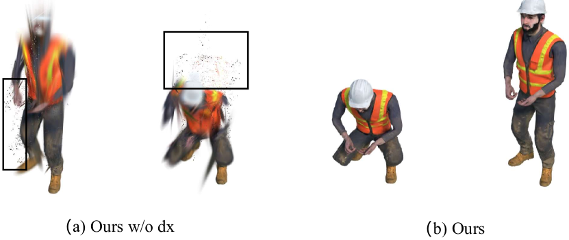
Figure 12: Visualization of ablation study about $\phi_{x}$.

A.3 More Ablation Studies and Discussions

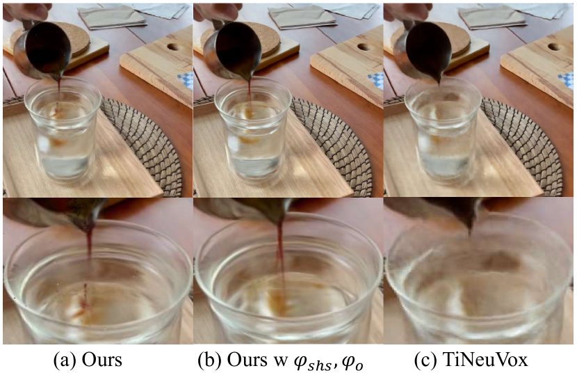
Figure 13: Visualization of ablation study in $\phi_{\mathcal{C}}$ and $\phi_{\mathcal{\alpha}}$ comparing with TiNeuVox [6].

Position Deformation.

We find that removing the output of the position deformation head can also model the object motion. It is mainly because leaving some 3D Gaussians in the dynamic part, keeping them small in shape, and then scaling them up at a certain timestamp can also model the dynamic part. However, this approach can only model coarse object motion and lost potential for tracking. The visualization is shown in Fig. 12.

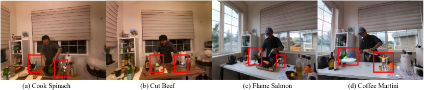
Figure 14: More visualization of composition with 4D Gaussians. (a) Composition with Punch and Standup. (b) Composition with Lego and Trex. (c) Composition with Hellwarrior and Mutant. (d) Composition with Bouncingballs and Jumpingjack.

Composition with 4D Gaussians.

We provide more visualization in composition with 4D Gaussians with Fig. 14. This work only proposes a naive approach to transformation. It is worth noting that when applying the rotation of the scenes, 3D Gaussian’s rotation quaternion $q$ and scaling coefficient $s$ need to be considered. Meanwhile, some interpolation methods should be applied to enlarge or reduce 4D Gaussians.

Color and Opacity’s Deformation.

When encountered with fluid or non-rigid motion, we adopt another two output MLP decoder $\phi_{\mathcal{C}}$, $\phi_{\alpha}$ to compute the deformation of 3D Gaussian’s color and opacity $\Delta\mathcal{C}=\phi_{\mathcal{C}}(f_{d})$, $\Delta\alpha=\phi_{\mathcal{\alpha}}(f_{d})$. Tab. 8 and Fig. 13 show the results in comparison with TiNeuVox [6]. However, it is worth noting that modeling Gaussian color and opacity change may cause irrational shape changes when rendering novel views. i.e. the Gaussians on the surface should move with other Gaussians but stay in the place and the color is changed, making the tracking difficult to achieve.

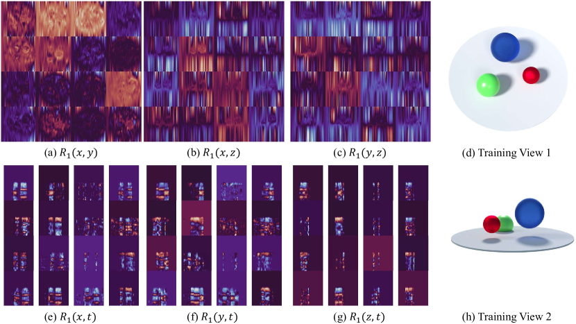
Figure 15: More visualization of the HexPlane voxel grids $R(i,j)$ in bouncing balls. (a)-(c), (e)-(f) stand for visualization of $R_{1}(i,j)$, where grids resolution equals to 64$\times$64.

Spatial-temporal Structure Encoder.

We have explored why 4D-GS can achieve such a fast convergence speed and rendering quality. As shown in Fig. 15, we visualize the full features of $R_{1}$ in bouncingballs. It’s explicit that in the $R_{1}(x,y)$ plane, the spatial structure of the scenes is encoded. Similarily, $R_{1}(x,z)$ and $R_{1}(y,z)$ also show different view structure features. Meanwhile, temporal voxel grids $R_{1}(x,t),R_{1}(y,t)$ and $R_{1}(z,t)$ also show the integrated motion of the scenes, where large motions always stand for explicit features. So, it seems that the proposed HexPlane module encodes the features of spatial and temporal information.

A.4 More Limitations

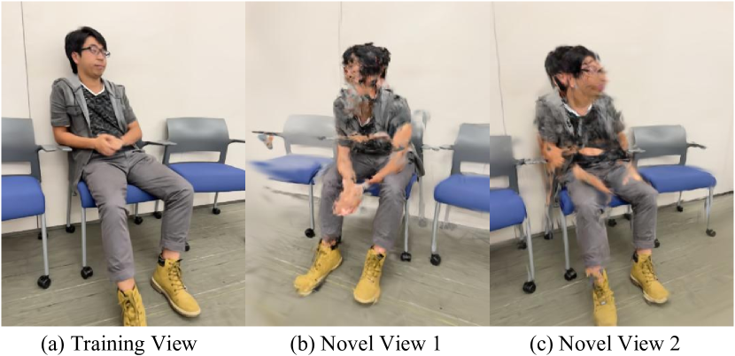
Figure 16: Novel view rendering results in the iPhone datasets [10].

Monocular Dynamic Scene Reconstruction.

In monocular settings, input data are sparse from both cameration pose and timestamp dimensions. This may cause the local minima of overfitting with training images in some complicated scenes. As shown in Fig. 16, though 4D-GS can render relatively high quality in the training set, the strong overfitting effects of the proposed model cause the failure of rendering novel views. To solve the problem, more priors such as depth supervision or optical flow may be needed.

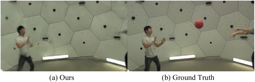
Figure 17: Rendering results on sports dataset [13] also used in Dynamic3DGS [21].

Large Motion Modeling with Multi-Camera Settings.

In the DyNeRF [17]’s dataset, all the motion parts of the scene are not very large and the multi-view camera setup also provides a dense sampling of the scene. That is the reason why 4D-GS can perform a relatively high rendering quality. However, in large motion such as sports datasets [13] used in [21], 4DGS cannot fit well within short times as shown in Fig. 17. Online training [21, 1] or using information from other views like [18, 39] could be a better approach to solve the problem with multi-camera input.

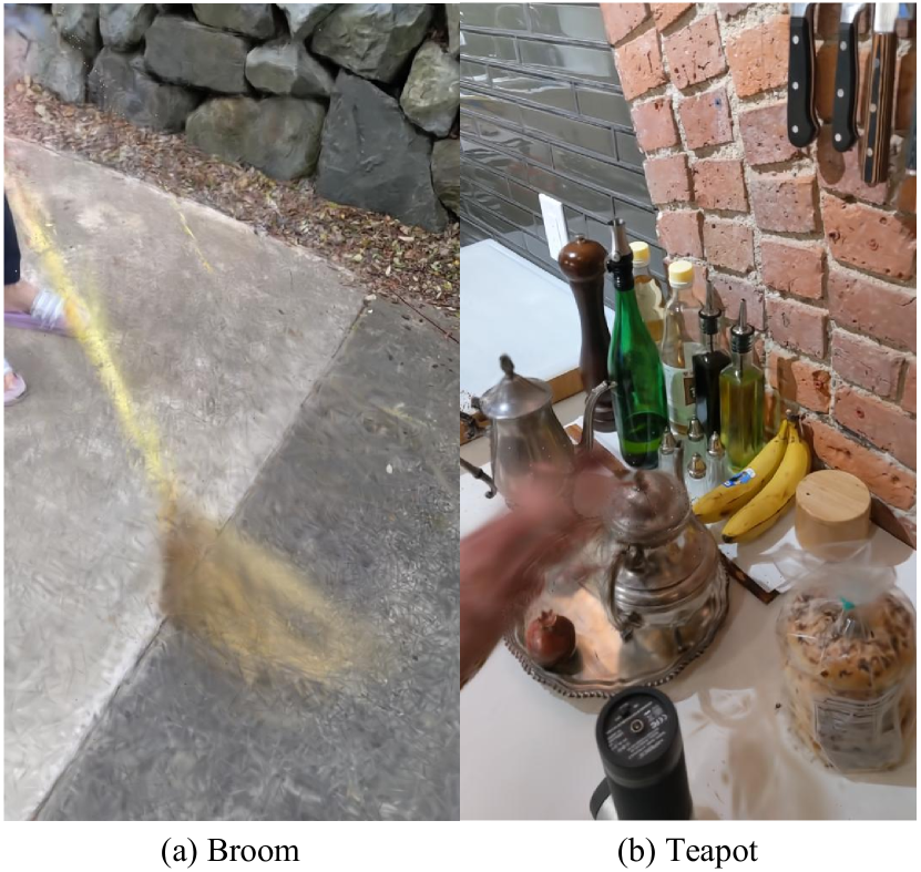
Figure 18: Failure cases of modeling large motions and dramatic scene changes. (a) The sudden motion of the broom makes optimization harder. (b) Teapots have large motion and a hand is entering/leaving the scene.

Large Motion Modeling with Monocular Settings.

4D-GS uses a deformation field network to model the motion of 3D Gaussians, which may fail in modeling large motions or dramatic scene changes. This phenomenon is also observed in previous NeRF-based methods [6, 28, 25, 17], producing blurring results. Fig. 18 shows some failed samples. Exploring more useful priors could be a promising future direction.

References

- Abou-Chakra et al. [2022] Jad Abou-Chakra, Feras Dayoub, and Niko Sünderhauf. Particlenerf: Particle based encoding for online neural radiance fields in dynamic scenes. arXiv preprint arXiv:2211.04041, 2022.
- Attal et al. [2023] Benjamin Attal, Jia-Bin Huang, Christian Richardt, Michael Zollhoefer, Johannes Kopf, Matthew O’Toole, and Changil Kim. Hyperreel: High-fidelity 6-dof video with ray-conditioned sampling. In Proceedings of the IEEE/CVF Conference on Computer Vision and Pattern Recognition, pages 16610–16620, 2023.
- Barron et al. [2021] Jonathan T Barron, Ben Mildenhall, Matthew Tancik, Peter Hedman, Ricardo Martin-Brualla, and Pratul P Srinivasan. Mip-nerf: A multiscale representation for anti-aliasing neural radiance fields. In Proceedings of the IEEE/CVF International Conference on Computer Vision, pages 5855–5864, 2021.
- Cao and Johnson [2023] Ang Cao and Justin Johnson. Hexplane: A fast representation for dynamic scenes. In Proceedings of the IEEE/CVF Conference on Computer Vision and Pattern Recognition, pages 130–141, 2023.
- Drebin et al. [1988] Robert A Drebin, Loren Carpenter, and Pat Hanrahan. Volume rendering. ACM Siggraph Computer Graphics, 22(4):65–74, 1988.
- Fang et al. [2022] Jiemin Fang, Taoran Yi, Xinggang Wang, Lingxi Xie, Xiaopeng Zhang, Wenyu Liu, Matthias Nießner, and Qi Tian. Fast dynamic radiance fields with time-aware neural voxels. In SIGGRAPH Asia 2022 Conference Papers, pages 1–9, 2022.
- Fridovich-Keil et al. [2022] Sara Fridovich-Keil, Alex Yu, Matthew Tancik, Qinhong Chen, Benjamin Recht, and Angjoo Kanazawa. Plenoxels: Radiance fields without neural networks. In Proceedings of the IEEE/CVF Conference on Computer Vision and Pattern Recognition, pages 5501–5510, 2022.
- Fridovich-Keil et al. [2023] Sara Fridovich-Keil, Giacomo Meanti, Frederik Rahbæk Warburg, Benjamin Recht, and Angjoo Kanazawa. K-planes: Explicit radiance fields in space, time, and appearance. In Proceedings of the IEEE/CVF Conference on Computer Vision and Pattern Recognition, pages 12479–12488, 2023.
- Gao et al. [2021] Chen Gao, Ayush Saraf, Johannes Kopf, and Jia-Bin Huang. Dynamic view synthesis from dynamic monocular video. In Proceedings of the IEEE/CVF International Conference on Computer Vision, pages 5712–5721, 2021.
- Gao et al. [2022a] Hang Gao, Ruilong Li, Shubham Tulsiani, Bryan Russell, and Angjoo Kanazawa. Monocular dynamic view synthesis: A reality check. Advances in Neural Information Processing Systems, 35:33768–33780, 2022a.
- Gao et al. [2022b] Xiangjun Gao, Jiaolong Yang, Jongyoo Kim, Sida Peng, Zicheng Liu, and Xin Tong. Mps-nerf: Generalizable 3d human rendering from multiview images. IEEE Transactions on Pattern Analysis and Machine Intelligence, 2022b.
- Guo et al. [2023] Xiang Guo, Jiadai Sun, Yuchao Dai, Guanying Chen, Xiaoqing Ye, Xiao Tan, Errui Ding, Yumeng Zhang, and Jingdong Wang. Forward flow for novel view synthesis of dynamic scenes. In Proceedings of the IEEE/CVF International Conference on Computer Vision, pages 16022–16033, 2023.
- Joo et al. [2015] Hanbyul Joo, Hao Liu, Lei Tan, Lin Gui, Bart Nabbe, Iain Matthews, Takeo Kanade, Shohei Nobuhara, and Yaser Sheikh. Panoptic studio: A massively multiview system for social motion capture. In Proceedings of the IEEE International Conference on Computer Vision, pages 3334–3342, 2015.
- Kerbl et al. [2023] Bernhard Kerbl, Georgios Kopanas, Thomas Leimkühler, and George Drettakis. 3d gaussian splatting for real-time radiance field rendering. ACM Transactions on Graphics (ToG), 42(4):1–14, 2023.
- Keselman and Hebert [2022] Leonid Keselman and Martial Hebert. Approximate differentiable rendering with algebraic surfaces. In European Conference on Computer Vision, pages 596–614. Springer, 2022.
- Keselman and Hebert [2023] Leonid Keselman and Martial Hebert. Flexible techniques for differentiable rendering with 3d gaussians. arXiv preprint arXiv:2308.14737, 2023.
- Li et al. [2022] Tianye Li, Mira Slavcheva, Michael Zollhoefer, Simon Green, Christoph Lassner, Changil Kim, Tanner Schmidt, Steven Lovegrove, Michael Goesele, Richard Newcombe, et al. Neural 3d video synthesis from multi-view video. In Proceedings of the IEEE/CVF Conference on Computer Vision and Pattern Recognition, pages 5521–5531, 2022.
- Lin et al. [2023] Haotong Lin, Sida Peng, Zhen Xu, Tao Xie, Xingyi He, Hujun Bao, and Xiaowei Zhou. High-fidelity and real-time novel view synthesis for dynamic scenes. In SIGGRAPH Asia Conference Proceedings, 2023.
- Liu et al. [2019] Xingyu Liu, Mengyuan Yan, and Jeannette Bohg. Meteornet: Deep learning on dynamic 3d point cloud sequences. In Proceedings of the IEEE/CVF International Conference on Computer Vision, pages 9246–9255, 2019.
- Liu et al. [2023] Yu-Lun Liu, Chen Gao, Andreas Meuleman, Hung-Yu Tseng, Ayush Saraf, Changil Kim, Yung-Yu Chuang, Johannes Kopf, and Jia-Bin Huang. Robust dynamic radiance fields. In Proceedings of the IEEE/CVF Conference on Computer Vision and Pattern Recognition, pages 13–23, 2023.
- Luiten et al. [2024] Jonathon Luiten, Georgios Kopanas, Bastian Leibe, and Deva Ramanan. Dynamic 3d gaussians: Tracking by persistent dynamic view synthesis. In 3DV, 2024.
- Mildenhall et al. [2021] Ben Mildenhall, Pratul P Srinivasan, Matthew Tancik, Jonathan T Barron, Ravi Ramamoorthi, and Ren Ng. Nerf: Representing scenes as neural radiance fields for view synthesis. Communications of the ACM, 65(1):99–106, 2021.
- Müller et al. [2022] Thomas Müller, Alex Evans, Christoph Schied, and Alexander Keller. Instant neural graphics primitives with a multiresolution hash encoding. ACM Transactions on Graphics (ToG), 41(4):1–15, 2022.
- Park et al. [2021a] Keunhong Park, Utkarsh Sinha, Jonathan T Barron, Sofien Bouaziz, Dan B Goldman, Steven M Seitz, and Ricardo Martin-Brualla. Nerfies: Deformable neural radiance fields. In Proceedings of the IEEE/CVF International Conference on Computer Vision, pages 5865–5874, 2021a.
- Park et al. [2021b] Keunhong Park, Utkarsh Sinha, Peter Hedman, Jonathan T Barron, Sofien Bouaziz, Dan B Goldman, Ricardo Martin-Brualla, and Steven M Seitz. Hypernerf: A higher-dimensional representation for topologically varying neural radiance fields. arXiv preprint arXiv:2106.13228, 2021b.
- Paszke et al. [2019] Adam Paszke, Sam Gross, Francisco Massa, Adam Lerer, James Bradbury, Gregory Chanan, Trevor Killeen, Zeming Lin, Natalia Gimelshein, Luca Antiga, et al. Pytorch: An imperative style, high-performance deep learning library. Advances in neural information processing systems, 32, 2019.
- Peng et al. [2023] Sida Peng, Yunzhi Yan, Qing Shuai, Hujun Bao, and Xiaowei Zhou. Representing volumetric videos as dynamic mlp maps. In Proceedings of the IEEE/CVF Conference on Computer Vision and Pattern Recognition, pages 4252–4262, 2023.
- Pumarola et al. [2021] Albert Pumarola, Enric Corona, Gerard Pons-Moll, and Francesc Moreno-Noguer. D-nerf: Neural radiance fields for dynamic scenes. In Proceedings of the IEEE/CVF Conference on Computer Vision and Pattern Recognition, pages 10318–10327, 2021.
- Qi et al. [2017a] Charles R Qi, Hao Su, Kaichun Mo, and Leonidas J Guibas. Pointnet: Deep learning on point sets for 3d classification and segmentation. In Proceedings of the IEEE conference on computer vision and pattern recognition, pages 652–660, 2017a.
- Qi et al. [2017b] Charles Ruizhongtai Qi, Li Yi, Hao Su, and Leonidas J Guibas. Pointnet++: Deep hierarchical feature learning on point sets in a metric space. Advances in neural information processing systems, 30, 2017b.
- Rückert et al. [2022] Darius Rückert, Linus Franke, and Marc Stamminger. Adop: Approximate differentiable one-pixel point rendering. ACM Transactions on Graphics (ToG), 41(4):1–14, 2022.
- Schonberger and Frahm [2016a] Johannes L Schonberger and Jan-Michael Frahm. Structure-from-motion revisited. In Proceedings of the IEEE conference on computer vision and pattern recognition, pages 4104–4113, 2016a.
- Schonberger and Frahm [2016b] Johannes L Schonberger and Jan-Michael Frahm. Structure-from-motion revisited. In Proceedings of the IEEE conference on computer vision and pattern recognition, pages 4104–4113, 2016b.
- Shao et al. [2023] Ruizhi Shao, Zerong Zheng, Hanzhang Tu, Boning Liu, Hongwen Zhang, and Yebin Liu. Tensor4d: Efficient neural 4d decomposition for high-fidelity dynamic reconstruction and rendering. In Proceedings of the IEEE/CVF Conference on Computer Vision and Pattern Recognition, pages 16632–16642, 2023.
- Song et al. [2023] Liangchen Song, Anpei Chen, Zhong Li, Zhang Chen, Lele Chen, Junsong Yuan, Yi Xu, and Andreas Geiger. Nerfplayer: A streamable dynamic scene representation with decomposed neural radiance fields. IEEE Transactions on Visualization and Computer Graphics, 29(5):2732–2742, 2023.
- Sun et al. [2022] Cheng Sun, Min Sun, and Hwann-Tzong Chen. Direct voxel grid optimization: Super-fast convergence for radiance fields reconstruction. In Proceedings of the IEEE/CVF Conference on Computer Vision and Pattern Recognition, pages 5459–5469, 2022.
- Wang et al. [2023a] Feng Wang, Zilong Chen, Guokang Wang, Yafei Song, and Huaping Liu. Masked space-time hash encoding for efficient dynamic scene reconstruction. Advances in neural information processing systems, 2023a.
- Wang et al. [2023b] Feng Wang, Sinan Tan, Xinghang Li, Zeyue Tian, Yafei Song, and Huaping Liu. Mixed neural voxels for fast multi-view video synthesis. In Proceedings of the IEEE/CVF International Conference on Computer Vision, pages 19706–19716, 2023b.
- Wang et al. [2021] Qianqian Wang, Zhicheng Wang, Kyle Genova, Pratul P Srinivasan, Howard Zhou, Jonathan T Barron, Ricardo Martin-Brualla, Noah Snavely, and Thomas Funkhouser. Ibrnet: Learning multi-view image-based rendering. In Proceedings of the IEEE/CVF Conference on Computer Vision and Pattern Recognition, pages 4690–4699, 2021.
- Wang et al. [2023c] Yiming Wang, Qin Han, Marc Habermann, Kostas Daniilidis, Christian Theobalt, and Lingjie Liu. Neus2: Fast learning of neural implicit surfaces for multi-view reconstruction. In Proceedings of the IEEE/CVF International Conference on Computer Vision, pages 3295–3306, 2023c.
- Wang et al. [2004] Zhou Wang, Alan C Bovik, Hamid R Sheikh, and Eero P Simoncelli. Image quality assessment: from error visibility to structural similarity. IEEE transactions on image processing, 13(4):600–612, 2004.
- Xu et al. [2022a] Qingshan Xu, Weihang Kong, Wenbing Tao, and Marc Pollefeys. Multi-scale geometric consistency guided and planar prior assisted multi-view stereo. IEEE Transactions on Pattern Analysis and Machine Intelligence, 45(4):4945–4963, 2022a.
- Xu et al. [2022b] Qiangeng Xu, Zexiang Xu, Julien Philip, Sai Bi, Zhixin Shu, Kalyan Sunkavalli, and Ulrich Neumann. Point-nerf: Point-based neural radiance fields. In Proceedings of the IEEE/CVF Conference on Computer Vision and Pattern Recognition, pages 5438–5448, 2022b.
- Yang et al. [2023] Zeyu Yang, Hongye Yang, Zijie Pan, Xiatian Zhu, and Li Zhang. Real-time photorealistic dynamic scene representation and rendering with 4d gaussian splatting. arXiv preprint arXiv:2310.10642, 2023.
- Yi et al. [2023] Taoran Yi, Jiemin Fang, Xinggang Wang, and Wenyu Liu. Generalizable neural voxels for fast human radiance fields. arXiv preprint arXiv:2303.15387, 2023.
- Yifan et al. [2019] Wang Yifan, Felice Serena, Shihao Wu, Cengiz Öztireli, and Olga Sorkine-Hornung. Differentiable surface splatting for point-based geometry processing. ACM Transactions on Graphics (TOG), 38(6):1–14, 2019.
- Yu et al. [2018] Lequan Yu, Xianzhi Li, Chi-Wing Fu, Daniel Cohen-Or, and Pheng-Ann Heng. Pu-net: Point cloud upsampling network. In Proceedings of the IEEE conference on computer vision and pattern recognition, pages 2790–2799, 2018.
- Zhang et al. [2020] Kai Zhang, Gernot Riegler, Noah Snavely, and Vladlen Koltun. Nerf++: Analyzing and improving neural radiance fields. arXiv preprint arXiv:2010.07492, 2020.
- Zhang et al. [2018] Richard Zhang, Phillip Isola, Alexei A Efros, Eli Shechtman, and Oliver Wang. The unreasonable effectiveness of deep features as a perceptual metric. In Proceedings of the IEEE conference on computer vision and pattern recognition, pages 586–595, 2018.
- Zwicker et al. [2001] Matthias Zwicker, Hanspeter Pfister, Jeroen Van Baar, and Markus Gross. Surface splatting. In Proceedings of the 28th annual conference on Computer graphics and interactive techniques, pages 371–378, 2001.