The quest of CMB spectral distortions to probe the scalar-induced gravitational wave background interpretation in PTA data

Abstract

Gravitational Waves (GW) sourced by second-order primordial curvature fluctuations are among the favoured models fitting the recent Pulsar Timing Array (PTA) measurement of a Stochastic GW Background (SGWB). We study how spectral distortions (SDs) and anisotropies of the Cosmic Microwave Background (CMB) can constrain such scalar fluctuations. Whereas COBE FIRAS data have no sufficient sensitivity to probe the PTA lognormal hypothesis, we show how future PIXIE-like experiments can detect the CMB SDs from the scalar-induced interpretation of the SGWB in PTA data. We finally show how the transformative synergy between PTA data and future CMB SD measurements is important for reconstructing primordial fluctuations at these small scales.

Introduction. One of the goals of modern cosmology is the characterization of the primordial power spectrum (PPS) of the curvature perturbations $\mathcal{P}(k)$ generated during inflation. The long wavelength quantum fluctuations amplified during inflation classicalize and re-enter the Hubble radius in the radiation and matter eras, providing the initial seeds for the gravitational instability in the large scale structure of the Universe.

The most stringent constraints on the PPS arise from Cosmic Microwave Background (CMB) anisotropies measurements, revealing a near scale invariant, slightly red-tilted, PPS on very large scales within the range $[0.001,\,0.1]\,{\rm Mpc}^{-1}$. The Planck DR3 data constrain the amplitude $A_{s}$ of the PPS at $k=0.05\,{\rm Mpc}^{-1}$ and its spectral index to $\ln\left(10^{10},A_{s}\right)=3.044\pm 0.014$ and $n_{s}=0.9649\pm 0.0042$ at 68% CL, respectively Planck:2018jri . Galaxy surveys can extend these constraints to ${\cal O}(1)\,{\rm Mpc}^{-1}$, but smaller scales remain largely unconstrained.

Recent observations of a Stochastic Gravitational Wave Background (SGWB) at nHz by Pulsar Timing Arrays (PTA) NANOGrav:2023gor ; Reardon:2023gzh ; EPTA:2023fyk ; Xu:2023wog have sparked a significant interest in the PPS at much smaller scales, since scalar fluctuations can generate such a SGWB at second order in perturbation theory Matarrese:1997ay ; Ananda:2006af ; Baumann:2007zm at scales $[10^{7},\,10^{9}]\,{\rm Mpc}^{-1}$. Recent studies suggest that such a Scalar Induced Gravitational Wave Background (SIGWB) could provide a viable explanation for the PTA detection and might be favored over many other candidates from a Bayesian perspective NANOGrav:2023hvm ; EPTA:2023xxk (see however NANOGrav:2023hvm ; EPTA:2023xxk ; Franciolini:2023pbf ; Figueroa:2023zhu ; Ellis:2023oxs for a discussion of potential PBH overproduction associated to this SIGWB explanation and  Franciolini:2023pbf ; Figueroa:2023zhu ; Ellis:2023oxs ; Liu:2023ymk ; Wang:2023ost ; Cai:2023dls for alternative analyses). If substantiated, PTA measurements could provide valuable insights into the later stages of inflation, with profound implications for theoretical models.

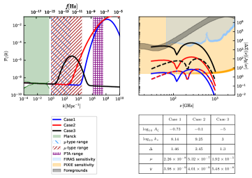
Figure 1: [Left] Illustrative primordial spectra together with constraints from Planck and sensitivity ranges of $y$ and $\mu$-type distortions and PTA. [Right] Corresponding $\mu$ (solid lines) and $y$-type (dashed lines) SD signals as functions of the frequency $\nu$ of the CMB black-body spectrum, compared to the sensitivity of FIRAS and PIXIE as well as to the total contribution of foregrounds. $\mu$ and $y$ distortions are computed by adopting the window functions of PIXIE. In the Table, we report the fiducial parameters for each case.

It is therefore of utmost importance to devise further tests of this hypothesis, and, as is often the case in cosmology, the synergy with other probes of the PPS becomes invaluable. In this context, it is noteworthy that the dissipation into acoustic waves of curvature perturbations responsible for the SIGWB inevitably induces spectral distortions (SDs) of the CMB spectrum by mixing photons with different temperatures Hu:1994bz ; Chluba:2012we ; Clesse:2014pna ; Chluba:2015bqa ; Byrnes:2018txb ; Unal:2020mts ; Schoneberg:2020nyg . The scales tested by SDs lie within the range $\sim[1,\,10^{4}]\,{\rm Mpc}^{-1}$, effectively bridging the observational gap between CMB anisotropies and PTA, thereby extending our leverage in constraining the PPS, as shown in Fig. 1. Furthermore, since alternative interpretations of PTA signals, such as those attributed to SMBHs, phase transitions, or cosmic strings do not predict significant SDs, CMB anisotropies and SDs offer an opportunity to falsify the SIGWB hypothesis underlying the PTA detection.

Motivation and data. In this study, we explore the implications of the SIGWB interpretation of recent PTA data NANOGrav:2023gor ; Reardon:2023gzh ; EPTA:2023fyk ; Xu:2023wog on the anisotropies and SDs of the CMB. We use Planck data for CMB anisotropies, and, for SDs, we consider both COBE FIRAS constraints Fixsen:1996nj and what can be achieved from future spectrometers, like PIXIE Kogut:2011xw or the concept presented in the ESA Voyage 2050 program Chluba:2019nxa . We use NANOGrav 15 publicly available data NANOGrav:2023gor for the recent PTA measurement of SGWB NANOGrav:2023gor ; Reardon:2023gzh ; EPTA:2023fyk ; Xu:2023wog .

Whereas the complementarity between CMB SDs and PTA data was previously discussed Byrnes:2018txb ; Unal:2020mts ; Schoneberg:2020nyg , our work is the first one where the synergy between the recent PTA detection of a SGWB  NANOGrav:2023gor ; Reardon:2023gzh ; EPTA:2023fyk ; Xu:2023wog and CMB SDs is studied quantitatively in a fully consistent Bayesian way by taking into account marginalization over foreground contamination and reionization effects. Our analysis also differs from previous approaches in technical details.

Instead of relying on the commonly employed window function approximation for calculating $\mu$ and $y$-type SDs Pajer:2012vz ; Chluba:2013dna , we rigorously compute them using the Green’s function method proposed in Chluba:2013vsa and implemented in the extension of the CLASS code Blas:2011rf introduced in  Lucca:2019rxf ; Fu:2020wkq .

The analysis. In our analysis, we adopt a straightforward yet widely used lognormal (LN) parameterization for a peak in the PPS Pi:2020otn which encapsulates its critical attributes, including amplitude, location, and width:

$$\mathcal{P}_{\rm LN}(k)= \frac{A_{\zeta}}{\sqrt{2\pi}\Delta}\exp\left[-\frac{\ln^{2}k/k_{*}}{2\Delta^{2}}\right].$$ (1)

While this parameterization may not capture the details of specific inflationary models across all scales, it enables us to draw generic conclusions and to establish connections with recent PTA analyses Dandoy:2023jot ; NANOGrav:2023hvm ; Reardon:2023gzh ; EPTA:2023xxk ; Figueroa:2023zhu ; Franciolini:2023pbf , which also employed the parameterization in Eq. (1). We will comment on possible extensions in the Conclusions. We add this LN peak to the $\Lambda$CDM power-law spectrum of curvature perturbation parametrized by $(A_{s},n_{s})$.

Within the LN parameterization, we adopt 3 fiducials, whose parameters are reported in Fig. 1 together with their $\mu$ and $y$ SD signals. We chose them as follows:

• Case 1 is the maximum likelihood sample from the MCMC chains of the SIGWB analysis Footnote1 of the NG15 collaboration NANOGrav:2023hvm , which we take as a representative PTA dataset. It produces an SD signal that is indistinguishable from a near scale invariant PPS.

• Case 2 lies well within the 68% CL contours of NG15, and produces a SD signal that is within the reach of the planned sensitivity of PIXIE.

• Case 3 peaks at the center of the window function of both FIRAS and PIXIE, and produces an SD signal that will be detected PIXIE at high statistical significance, but weak enough to be allowed by FIRAS. Being outside their sensitivity range, the associated GW signal cannot explain the recent PTA detection, which would be ascribed to either SMBHs or other models.

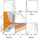
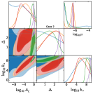
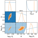
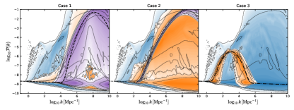
Figure 2: [Top] 1D and 2D posterior distributions of the LN parameters, and 1D distribution for the derived parameter $\mu$. [Bottom] Predictive posterior distributions for $\mathcal{P}_{\rm LN}(k)$.

The methodology of our MCMC analyses and forecasts is described in detail in the Supplemental Materials. There, we also report the priors on the parameters and explain our method of marginalization over nuisance and foreground parameters in the case of SDs. In addition to present 1d and 2d constraints on the model parameters, we also plot the predictive posterior distribution (PPD) of $\mathcal{P}(k)$, allowing a straightforward visualization of the constraints on the PPS itself, which cannot be grasped from the triangle plots alone.

Constraints from FIRAS and Planck. For all the three cases studied, FIRAS data are not very informative, as can be seen from the blue contours in the triangle plots in Fig. 2, and in combination with Planck can only exclude some regions of the parameter space - in particular, Planck provides a lower limit for $k_{*}$. Because our prior on $k_{*}$ allows the peak in the PPS to also fall completely outside the window function of FIRAS, the amplitude $A_{\zeta}$ is unconstrained after marginalizing over the other parameters. However, we can clearly see a scale dependent bound on $A_{\zeta}$ in the 2D plane $\log_{10}\,A_{\zeta}$ vs $\log_{10}\,k_{*}$. The PPD of $\mathcal{P}(k)$ depicts tight constraints at the largest scales tested by Planck Planck:2018jri . Moving to intermediate scales, within the window function of FIRAS, the upper limit on the amplitude is roughly $A_{\zeta}\lesssim 10^{-4}$. At smaller scales, to which FIRAS is not sensitive, $\mathcal{P}(k)$ becomes unbounded. Our results are consistent with those of previous analyses obtained with simpler approximations Byrnes:2018txb ; Unal:2020mts .

Forecasts for PIXIE plus Planck. Our PIXIE forecasts in combination with Planck are shown in Fig. 2, on top of the constraints from FIRAS. PIXIE and Planck cannot detect the signal for Case 1, mainly due to the smallness of $\mu$ predicted. Whereas, due to the much better sensitivity, the constraints on the amplitude do improve, the bump in the power spectrum is located at such small scales and does not contribute to the SD signal. Case 2 is perhaps the most interesting one (see the Supplemental Material for more details). We see that, despite the predicted $\mu$ being well within the reach of the nominal PIXIE sensitivity, i.e. $\mu_{\rm PIXIE}\lesssim 2\times 10^{-8}$ as quoted in Kogut:2011xw , the model parameters are not well constrained and, although the reconstructed PPS does show a hint of a deviation from near scale invariance, the bump is not detected and the PPS is still consistent with a near scale invariant one. $\mu$ and $y$ distortions are indeed consistent with the minimal signal predicted by $\Lambda$CDM, although the posterior distribution of $\mu$ does show a peak around the fiducial value of $\mu=5.32\times 10^{-7}$. This agrees with previous studies (see e.g. Fu:2020wkq ) that indicate that the nominal sensitivity is degraded by almost an order of magnitude when consistently including all the foregrounds that are expected to act as nuisance for PIXIE SathyanarayanaRao:2015vgh ; Desjacques:2015yfa ; Mashian:2016bry ; Abitbol:2017vwa ; Rotti:2020tlo ; Zelko:2020ojo . As seen from the red contours in Fig. 2, removing foregrounds would allow a signifcant detection of $\mu=\left(\,5.27\pm 0.09\,\right)\times 10^{-7}$ at 68% CL, although this would not translate into a statistically significant deviation from near scale invariance, and the constraints on $\mathcal{P}(k)$ are nearly unchanged. We thus learn two valuable lessons. On one hand, foregrounds can degrade the sensitivity of SD experiments to the PPS. On the other, even after foreground removal, if the SD signal is not strong enough so that both $\mu$ and $y$ distortions are detected, it becomes complicated to detect with high confidence models of a peak in the PPS like Eq. (1), due to the parameter degeneracies. While estimating $\mu$ and $y$ distortions can quickly indicate if there is hope to detect a signal with future experiments (see e.g. Byrnes:2018txb ; Unal:2020mts ), our analyses highlight the importance of adopting a rigorous forecasting procedure to assess conclusions about a given model of a peak in the PPS. This is one of the main results of this work. Finally, the SD signal from Case 3 is so loud that PIXIE can detect $\mu=\left(\,1.92\pm 0.02\,\right)\times 10^{-5}$ and $y=\left(\,4.9^{+1.7}_{-3.1}\,\right)\times 10^{-8}$ at 68%CL. As shown in the corresponding triangle plot, while some degeneracies between the model parameters still show up, the model parameters can be very well constrained and a near scale invariant PPS is excluded with extremely high confidence in the range $k\in[10^{2},\,10^{4}]\,{\rm Mpc}^{-1}$.

Synergy with PTA. Let us now discuss the synergy between future SD experiments and PTA data. To do that, we take the multi-dimensional posterior distribution on the LN parameters $(\log_{10}\,A_{\zeta},\,\Delta,\,\log_{10}k_{*})$ from the public chains of the NG15 analysis of the SIGWB and use it as input for our forecast for PIXIE. We discussed how Case 1 cannot be detected by PIXIE, as its SD signal is too weak. However, the parameter space allowed by NG15 still contains some regions producing a large $\mu$-type distortion, which will be ruled out by PIXIE, as seen from the purple contours in the triangle plot for Case 1. The improvement in the constraints is more dramatic for Case 2. Despite consistently marginalizing over foregrounds and temperature shifts, the fiducial parameters can be recovered and accurately constrained. The synergy between SDs and PTA would thus be extremely helpful to probe large deviations in the PPS from a power-law shape beyond the detection of $\mu$.

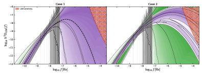
Figure 3: Derived constraints on the spectral shape of the SGWB from the NG15 analysis (green) as well as the forecasts for the PIXIE + Planck + NG15 in Case 2 (purple). We also plot the NG15 violin plots and the LISA power-law sensitivity curve at higher frequencies.

Conclusions. Motivated by the recent detection of an SGWB by PTA experiments, and its possible scalar-induced nature NANOGrav:2023gor ; Reardon:2023gzh ; EPTA:2023fyk ; Xu:2023wog ; NANOGrav:2023hvm ; EPTA:2023xxk , we investigated how future measurements of CMB SDs could probe the dissipation into acoustic waves ot these scalar perturbations producing the SGWB. We found that the parameter space consistent with PTA observations spans several orders of magnitude in $\mu$-type and $y$-type SD signals, with both small and large amplitudes. While COBE FIRAS data contribute minimally to the constraints within this range, future experiments as PIXIE hold great promise for probing this uncharted territory, especially when combined with PTA. Furthermore, we showed that an experiment like PIXIE will be able to bridge between the scales tested by CMB anisotropies and PTA, probing corners of the parameter space not accessible to either of them and thus a unique target of future SD experiments. Note also that our results are somewhat conservative, since more sensitive concepts than PIXIE have been proposed as future space experiments for CMB SDs Chluba:2019nxa .

We also identify promising avenues which go beyond the results presented in this paper:

Beyond the LN template. Our choice for the LN template as workshorse for our analysis has been dictated either for simplicity and because it has been chosen by the NANOGrav collaboration. Features beyond the LN template have been proposed, such as different infrared or ultraviolet slopes, large dips characteristic of ultra-slow-roll dynamics Balaji:2022zur , steep growth of the infrared tail beyond $k^{4}$, indicative of multifield scenarios Byrnes:2018txb ; Fumagalli:2020adf ; Palma:2020ejf ; Braglia:2020eai ; Fumagalli:2020nvq ; Braglia:2020taf ; Braglia:2022phb ; Cole:2022xqc , or large oscillations due to sharp features Fumagalli:2020adf ; Palma:2020ejf ; Braglia:2020eai ; Fumagalli:2020nvq ; Braglia:2020taf . Repeating our analyses with more realistic templates or direct numerical integration of inflationary equations can bridge the gap between data and fundamental theoretical parameters.

PBHs. A large peak in $\mathcal{P}(k)$ may lead to the formation of PBHs. A rough estimate of the threshold for (over)production of PBHs is $A_{\zeta}\sim\mathcal{O}(0.01-0.1)$. Our posteriors includes amplitudes much larger, raising questions about the overproduction of light PBHs. There are, however, several well known caveats that affect the quick estimates above and rose again to prominence after the PTA detection. The PBH abundance is strongly affected by the PBH formation criteria Gow:2020bzo ; Inomata:2023zup , the shape of the PPS Gow:2020cou , the accurate size of the physical horizon at formation DeLuca:2023tun , the equation of state (EOS) of the Universe at PBH formation Byrnes:2018clq and, notably, non-Gaussianities Ferrante:2022mui ; Gow:2022jfb ; Franciolini:2023pbf ; Inomata:2023drn . In particular, also the SIGWB would be modified upon including changes in the equation of state of the Universe Franciolini:2023wjm ; Balaji:2023ehk ; Harigaya:2023pmw and non-Gaussianities in the calculation of the SGWB Unal:2018yaa ; Adshead:2021hnm ; Ragavendra:2021qdu ; Li:2023xtl . Furthermore, PBHs would impact SDs also through their accretion Ali-Haimoud:2016mbv . A state of the art discussion of the resulting constraints which derives from PBH formation is beyond the scope of this work.

Other CMB SD imprints. Finally, although we have only considered the total intensity spectrum of the CMB, other SD observables such as $T-\mu$ correlation Pajer:2012vz ; Ozsoy:2021qrg ; Bianchini:2022dqh , SD anisotropies Zegeye:2021yml have been proved to provide valuable constraints on the shape of the PPS. Furthermore, also tensor perturbations directly source SDs Ota:2014hha ; Chluba:2014qia , although their signal is much weaker compared to the one explored in this paper. All such insights add to the prospects of testing the PPS with future SD experiments.

Our results also demonstrate that measuring an SD signal will advance our understanding of primordial physics and also hold significant implications for interpreting data from future space-based GW observatories, such as LISA LISA:2017pwj or BBO Crowder:2005nr -Decigo Kawamura:2006up , as displayed in Fig. 3. When analyzing current PTA data in terms of an LN peak, the predicted $\Omega_{\rm GW}$ from the posterior distribution of the model parameters intersects the sensitivity of future GW experiments. Adding information from SD anchors a SIGWB at large scales, so that its shape within the LISA sensitivity band is theoretically predicted. This theoretical prior can optimize the search of an SGWB at ${\rm mHz}$ frequencies, a key scientific target of LISA Bartolo:2016ami ; Caprini:2019egz ; LISACosmologyWorkingGroup:2022jok . We believe that such profound physical implications provide strong support for the science case of a future space based CMB spectrometer.

Acknowledgments. We thank Chris Byrnes, Jens Chluba, and Matteo Lucca for interesting discussions. We thank Chris Byrnes and Valerie Domcke for comments on a draft of this paper. MT acknowledges the funding by the European Union - NextGenerationEU, in the framework of the HPC project – “National Centre for HPC, Big Data and Quantum Computing” (PNRR - M4C2 - I1.4 - CN00000013 – CUP J33C22001170001)). MB thanks the Theoretical Physics Department of CERN and INAF/OAS Bologna, where part of this work was carried out, for hospitality. FF acknowledges financial support from the INFN InDark initiative and from the COSMOS network (www.cosmosnet.it) through the ASI (Italian Space Agency) Grants 2016-24-H.0 and 2016-24-H.1-2018, as well as 2020-9-HH.0 (participation in LiteBIRD phase A). We acknowledge the use of computational resources from the parallel computing cluster of the Open Physics Hub (https://site.unibo.it/openphysicshub/en) at the Physics and Astronomy Department in Bologna and from the INAF/OAS Bologna cluster. In this paper, we made use of the softwares CLASS Blas:2011rf , MontePython Brinckmann:2018cvx , GetDist Lewis:2019xzd and fgivenx fgivenx .

Note added.- While this project was near to completion, a related paper Cyr:2023pgw , also studying the capability of SDs to constrain $\mathcal{P}(k)$ and its relation to the recent PTA detection, appeared on the arXiv. Whereas we perform a MCMC Pixie-like forecast for a lognormal bump of curvature perturbations fitting PTA data, Ref.  Cyr:2023pgw discusses the accuracy in the SD theoretical calculation of different templates motivated by PTA data and explores the relevance of the additional dissipation of tensor fluctuations. Under the same assumptions, our results broadly agree with those of  Cyr:2023pgw .

Appendix A Supplemental materials

CMB spectral distortions. Here we briefly review the calculation of the SD signal MTthesis , focusing on the imprints of the shape of the PPS on $\mu$ and $y$-type distortions. The SD of the CMB $\Delta I$ can be decomposed as follows:

$$\Delta I(x)=\Delta I_{\rm SZ}(x)+\Delta I_{T}(x)+\Delta I_{\rm fg}(x)+\Delta I_{\rm exotic}+\Delta I_{\rm\Lambda CDM},$$ (2)

where $x$ is the dimensionless frequency $x=h\nu/(k_{B}T_{0})$, and the different terms represent contributions from late-time reionization $\Delta I_{\rm SZ}$, temperature shift $\Delta I_{\rm T}$, foregrounds $\Delta I_{\rm fg}$, possible exotic physics $\Delta I_{\rm exotic}$ and the minimal signal produced by $\Lambda$CDM $\Delta I_{\rm\Lambda CDM}$. Let us briefly comment on each of these term.

${\bf\Delta I_{\rm SZ}(x)}$ is the late-time Sunyaev-Zeldovich contribution from energetic reionized electrons that scatter CMB photons creating SDs. This term can be approximated as in Schoneberg:2020nyg :

$$\Delta I_{\rm SZ}(x)=\mathcal{N}x^{3}y_{\rm reio}Y(x).$$ (3)

${\bf\Delta I_{\rm T}}$ arises from the difference between the true CMB temperature $T$ and its reference value $T_{0}$:

$$\Delta I_{T}(x)=\mathcal{N}x^{3}\left[\Delta_{T}(1+\Delta_{T})G(x)+(\Delta_{T}^{2}/2)Y(x)\right],$$ (4)

where $\mathcal{N}=2(k_{B}T)^{3}/(hc)^{2}$, $G(x)=xe^{x}/(e^{x}-1)^{2}$, $Y(x)=G(x)[x(e^{x}+1)/(e^{x}-1)-4]$ and $\Delta_{T}=(T-T_{0})/T_{0}$.

${\bf\Delta I_{\rm fg}}$ encodes foreground contributions from the Galactic thermal dust, the Cosmic Infrared Background (CIB), synchrotron, free-free, spinning dust, and integrated CO emissions. A detailed description of this term and its implementation in MontePython can be found in Abitbol:2017vwa ; Schoneberg:2020nyg .

${\bf\Delta I_{\rm exotic}}$ contains the cosmological signal from exotic energy injections at high redshifts. As we are not interested in such Physics in this paper, we set it to $\Delta I_{\rm exotic}=0$.

Finally, ${\bf\Delta I_{\Lambda{\rm CDM}}}$ is the sum of two main contributions, i.e. adiabatic cooling of electrons and baryons and dissipation of acoustic waves. Since the former effect is not related to the PPS, we describe only the latter. The presence of primordial density fluctuations generated during inflation causes some regions of the primordial plasma to be hotter and denser than others. The various regions of the plasma at different temperatures are all represented by a black body spectrum. Photons diffuse from overdense to underdense regions and vice versa, generating an isotropization of the photon phase space distribution at small scales Silk:1967kq and CMB SDs Sunyaev:1970plh ; Daly:1991uob ; 10.1093/mnras/248.1.52 ; Hu:1994bz . The rate of the energy injected in the plasma due to the Silk damping is  Chluba:2013dna

$$\frac{\mathrm{d}Q}{\mathrm{d}t}\approx 4A^{2}\rho_{\gamma}\int\mathrm{d}k\,k\,\mathcal{P}(k)\,(\partial_{t}k^{-2}_{D})\,e^{-2(k/k_{D})^{2}},$$ (5)

where $k_{D}$ is the Silk-damping scale, $\rho_{\gamma}$ the photon density and $A\approx(1+(4/15)\rho_{\nu}/\rho_{r})^{-1}$. We therefore see that the energy rate is proportional to the PPS, which sets the initial condition for the photon perturbations in the Early Universe. In general, the total SD signal can be decomposed as the sum of three different types of SDs, namely $\mu$, $y$, and $g$, and some residual term $R(x)$ that represents all the SDs that are neither $\mu$, $y$ or $g$ distortions. Each contribution to the SD signal is characterized by an amplitude and a shape. The $y$ and $g$ shapes are denoted by $Y(x)$ and $G(x)$ respectively, while the $\mu$ shape is $M(x)=G(x)[0.4561-1/x]$. Therefore, $\Delta I_{\Lambda\rm CDM}$ can be written as

$$\Delta I_{\Lambda{\rm CDM}}(x)=gG(x)+\mu M(x)+yY(x)+R(x)$$ (6)

The SD amplitudes $\mu$, $y$, and $g$ are in general computed given the rate of the energy into photons $\mathrm{d}Q/\mathrm{d}t$ as:

$$a=\int_{0}^{\infty}\mathrm{d}z\frac{\mathrm{d}Q/\mathrm{d}t}{(1+z)H\rho_{\gamma}}\mathcal{J}_{a}(z),\qquad\text{for}\qquad a=\mu,y,g,$$ (7)

where $\mathcal{J}_{a}(z)$ describes how much of the injected energy creates an $a$-type SD at $z$. There are different ways to compute the visibility functions $\mathcal{J}_{a}(z)$. We compute them with the PCA method implemented in CLASS Lucca:2019rxf , in which $\mathcal{J}_{a}(z)$ are equal to the branching ratios of the Green’s function of the thermalization problem $G_{\rm th}$ and where $R(x)$ is the residual of $G_{\rm th}$ Chluba:2013vsa . In the acoustic waves dissipation case, the injected energy rate is given by Eq. (5) and therefore the SD amplitudes (7) become

$$a=\int\frac{\mathrm{d}k}{k}\,\mathcal{P}(k)\,W_{a}(k),$$ (8)

where we define the window functions $W_{a}(k)$ as

$$W_{a}(k)=4\,A^{2}\,k^{2}\,\int_{0}^{\infty}\mathrm{d}z\,\frac{(\partial_{t}k^{-2}_{D})\,e^{-2(k/k_{D})^{2}}}{H\,(1+z)}\,\mathcal{J}_{a}(z).$$ (9)

If the visibility functions $\mathcal{J}_{a}(z)$ are computed with the PCA method, numerical integration is typically required to calculate the window functions. However, it is possible to approximate analytically $\mathcal{J}_{a}(z)$ and perform a straightforward integration of Eq. (9). In this case, it turns out that the approximated $\mu$ window function has support $\sim[1,\,10^{4}]\,{\rm Mpc}^{-1}$ plotted in Fig. 1 Chluba:2013dna .

To visualize how $\mu$ and $y$ depend on the template parameters (1), we can approximate $W_{\mu,y}(k)$ to top-hat functions $W_{\mu,y}=A_{\mu,\,y}\times\Theta(k-k_{\rm min})\,\Theta(k_{\rm max}-k)$, where $A_{\mu,y}$ is some proportionality constant. In this case, the expressions for $\mu$ and $y$ (8) can be analytically integrated

$$\mu,\,y=\frac{A_{\mu,\,y}\,A_{\zeta}}{2}\,\left.\operatorname{Erf}\left(\frac{\ln k-\ln k_{*}}{\sqrt{2}\,\Delta}\right)\right|^{k^{\mu,\,y}_{\rm max}}_{k^{\mu,\,y}_{\rm min}}$$ (10)

The analytic approximation captures quite well the dependence of $\mu$ and $y$ on the LN parameters, except when the LN pivot scale is moved closer to the edges of the window function. We show this in Fig. 4, where, for simplicity, we compare the analytic result (setting $A_{\mu}=2.27$ following Byrnes:2018txb ) to the one computed with the PCA method implemented in CLASS assuming the window function of COBE FIRAS.

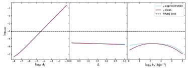
Figure 4: Comparison between the $\mu$ computed with the PCA method using CLASS and the simple analytic approximation (10). [Left] we vary $A_{\zeta}$ while keeping fixed $k_{*}=$100\text{\,}{\mathrm{Mpc}}^{-1}$$, $\Delta=1.5$. [Center] we vary $\Delta$ and we set $A_{\zeta}=10^{-6}$ and $k_{*}=$100\text{\,}{\mathrm{Mpc}}^{-1}$$. [Right] we vary $k_{*}$ while keeping fixed $A_{\zeta}=10^{-6}$ and $\Delta=1.5$.

CMB SD likelihoods and MCMC methodology. In this paper, we place constraints on the PPS through a Bayesian likelihood analysis. In order to use FIRAS constraints Fixsen:1996nj and to forecast the capability of a future PIXIE-like spectrometer Kogut:2011xw , we use the mock SD likelihood presented in Lucca:2019rxf and implemented in MontePython v3.5.0, which reads as follows

$$\ln\mathcal{L}_{\rm SD}=-\frac{1}{2}\sum_{i}\left(\frac{\Delta I_{\rm obs}(\nu_{i})-\Delta I_{\rm pred}(\nu_{i})}{\delta I(\nu_{i})}\right)^{2}\,.$$ (11)

Here $\Delta I(\nu_{i})$ is the detector sensitivity in the $i$-th frequency bin and $\Delta I_{\rm predicted}$ is the theoretical SD signal computed for some given model parameters. In the case of the LN bump in the PPS in Eq. (1), the parameters are $(A_{\zeta},k_{*},\Delta)$. For COBE FIRAS, in absence of a publicly available module with real data, we use the mock likelihood implemented in MontePython which is able to reproduce the upper limit on $\mu$ set by the COBE FIRAS Fixsen:1996nj . $\Delta I_{\rm obs}(\nu_{i})$ is the measured (fiducial) SD signal in the $i$-th frequency bin. We break the almost perfect degeneracy between $\mu$ and $\Delta_{T}$ (see Eq. (2)) using a Gaussian prior on $\Delta_{T}$ centered at $\overline{\Delta}_{T}=0$, with standard deviation $\sigma^{\rm FIRAS}_{{\Delta}_{T}}=2.2\times 10^{-4}$ and $\sigma^{\rm PIXIE}_{{\Delta}_{T}}=5\times 10^{-8}$ for COBE FIRAS and PIXIE, respectively, as done in  Fu:2020wkq . The Gaussian prior is essential to mitigate the degeneracy, especially in the Case 2, where the expected signal $\mu\approx 10^{-7}$ may be suppressed by a value of $\Delta_{T}$ of the same order. Eq. (4) shows that the term $\Delta I_{T}(x)$ includes a term proportional to the $g$-shape, $\Delta_{T}\cdot G(x)$, so that the overall amplitude multiplying $G(x)$ is the sum of $g$ and $\Delta_{T}$. Typically, the magnitude of $g$ is much smaller, around $10^{-10}$, compared to $\Delta_{T}$, making $g$-distortions negligible when considering temperature shifts. For this reason, we follow the default implementation in MontePython and neglect $g$-distortions in our analysis. The priors on $y_{\rm reio}$ and the other foreground parameters are also set following Schoneberg:2020nyg .

In order to include constraints on the PPS at $k\lesssim 0.1\,$/Mpc, we also fold in the constraining power of Planck data. Since FIRAS is implemented as a mock likelihood, in order to avoid combining real and simulated data, we use a mock likelihood for Planck reproducing the Planck 2018 $\Lambda$CDM results for cosmological parameters. The inverse Wishart log-likelihood $\ln\mathcal{L}_{\rm Planck}$ for TT, TE, and EE spectra covers a range of multipoles $\ell\in[2,2500]$, adopts a modified version of the sensitivity described in Schoneberg:2020nyg for the frequency channels 100, 143, and 217 GHz and covers a sky fraction $f_{\rm sky}=0.65$.

The results obtained with $\ln\mathcal{L}_{\rm SD}+\ln\mathcal{L}_{\rm Planck}$ by using a Metropolis-Hastings MCMC algorithm implemented in the MontePython sampler and by allowing to vary both the 6 $\Lambda$CDM and 3 LN parameters are shown in Fig. 5. These results are compared with those obtained by fixing the 6 $\Lambda$CDM cosmological parameters in Fig. 5. Given the good agreement that we find for this LN template, we proceed by keeping fixed the 6 $\Lambda$CDM cosmological parameters to reduce the computational cost of the MCMC analysis.

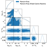
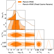
Figure 5: Comparison of the triangle plots obtained in the Case 1 for both a fixed and a varying $\Lambda$CDM cosmology. For simplicity, we restrict the priors on $\log_{10}A_{\zeta}$ and $\log_{10}k_{*}[${\mathrm{Mpc}}^{-1}$]$ within the ranges $[-10,-1]$ and $[-1,9]$ respectively.

In order to forecast the impact of future CMB SD measurements on the scalar-induced interpretation of PTA data, we compute the 3d marginalized posterior distribution of $(\log_{10}A_{\zeta},\log_{10}k_{*},\Delta)$ from the public chains of the NG15 analysis obtained by using the SIWGB associated to the LN model in Eq. (1). We then add the log-value of such normalized posterior to the total CMB log-likelihood $\ln\mathcal{L}_{\rm Planck}+\ln\mathcal{L}_{\rm SD}$.

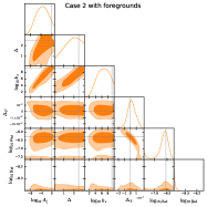
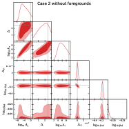
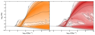
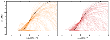
Figure 6: [Top ] triangle plots, [center] PPD for $\mathcal{P}(k)$, [bottom] and posterior samples for Case 2 varying (left) and keeping the foregrounds fixed to their values (right). The fiducial $\mathcal{P}(k)$ is plotted with a black dotted line.

The role of SD likelihoods for the PPS. We now discuss the relevance of SD likelihoods for the reconstruction of the PSS. In the top panels of Fig. 6, we add the derived posteriors on $\mu,\,y$ and $\Delta_{T}$ to the PIXIE forecast shown in Fig. 2. Fig. 6 shows how the constraints on $\mu$ are significantly affected by foregrounds, consistently with Schoneberg:2020nyg . By fixing the foregrounds, we get a significant detection $\mu=\left(\,5.3\pm 0.1\,\right)\times 10^{-7}$ at 68% CL. On the other hand, when we vary the foreground parameters in the analysis and marginalize over them, we only obtain a 95% CL upper bound on $\mu$, i.e. $8.5\times 10^{-7}$.

The role of foregrounds is instead different for the inference of the PPS by CMB SDs. Indeed, degeneracies among the LN parameters cannot be broken, even when foregrounds are removed and $\mu$ is detected with high statistical significance. This fact is easy to understand by looking at Eq. (8). Indeed, the detection of $\mu$ we can only constrain a specific combination of LN parameters, but not each of them individually. This clarifies why the PPD of $\mathcal{P}(k)$, despite hinting at a strong scale dependence at $\sim 1\sigma$ in the region $k\in[10^{2},\,10^{5}]\,{\rm Mpc}^{-1}$ (see the dark-shaded areas in Fig. 6), is consistent with a near scale invariant spectrum. To clarify the PPD, we also plot the posterior samples in the bottom panels of the Fig. 6. Both small peaks in the SD window and large ones at larger scales are admitted by the MCMC, as they yield the same value of $\mu$.

Measuring $y$ generated by the dissipation of the acoustic waves would break the degeneracies mentioned above, and assess the primordial origin of the SDs. However, $y$ generated by the dissipation of the acoustic waves in Case 2 is too small to be detected, regardless of the way we treat foregrounds in our forecast, see Fig. 1. This example can be compared to our forecast for Case 3 where $y$ is instead large enough to be detected by PIXIE, resulting in $\left(\,4.9^{+4.7}_{-4.3}\,\right)\times 10^{-8}$ at 95% CL. In that case, as shown in Fig. 2, the PPS parameters can be all constrained, and the $\mathcal{P}(k)$ can be reconstructed very well.

References

- (1) Y. Akrami et al. [Planck], Astron. Astrophys. 641, A10 (2020) doi:10.1051/0004-6361/201833887 [arXiv:1807.06211 [astro-ph.CO]].
- (2) G. Agazie et al. [NANOGrav], Astrophys. J. Lett. 951, no.1, L8 (2023) doi:10.3847/2041-8213/acdac6 [arXiv:2306.16213 [astro-ph.HE]].
- (3) D. J. Reardon, A. Zic, R. M. Shannon, G. B. Hobbs, M. Bailes, V. Di Marco, A. Kapur, A. F. Rogers, E. Thrane and J. Askew, et al. Astrophys. J. Lett. 951, no.1, L6 (2023) doi:10.3847/2041-8213/acdd02 [arXiv:2306.16215 [astro-ph.HE]].
- (4) J. Antoniadis et al. [EPTA], Astron. Astrophys. 678, A50 (2023) doi:10.1051/0004-6361/202346844 [arXiv:2306.16214 [astro-ph.HE]].
- (5) H. Xu, S. Chen, Y. Guo, J. Jiang, B. Wang, J. Xu, Z. Xue, R. N. Caballero, J. Yuan and Y. Xu, et al. Res. Astron. Astrophys. 23, no.7, 075024 (2023) doi:10.1088/1674-4527/acdfa5 [arXiv:2306.16216 [astro-ph.HE]].
- (6) S. Matarrese, S. Mollerach and M. Bruni, Phys. Rev. D 58, 043504 (1998) doi:10.1103/PhysRevD.58.043504 [arXiv:astro-ph/9707278 [astro-ph]].
- (7) K. N. Ananda, C. Clarkson and D. Wands, Phys. Rev. D 75, 123518 (2007) doi:10.1103/PhysRevD.75.123518 [arXiv:gr-qc/0612013 [gr-qc]].
- (8) D. Baumann, P. J. Steinhardt, K. Takahashi and K. Ichiki, Phys. Rev. D 76, 084019 (2007) doi:10.1103/PhysRevD.76.084019 [arXiv:hep-th/0703290 [hep-th]].
- (9) A. Afzal et al. [NANOGrav], Astrophys. J. Lett. 951, no.1, L11 (2023) doi:10.3847/2041-8213/acdc91 [arXiv:2306.16219 [astro-ph.HE]].
- (10) J. Antoniadis et al. [EPTA], [arXiv:2306.16227 [astro-ph.CO]].
- (11) G. Franciolini, A. Iovino, Junior., V. Vaskonen and H. Veermae, [arXiv:2306.17149 [astro-ph.CO]].
- (12) D. G. Figueroa, M. Pieroni, A. Ricciardone and P. Simakachorn, [arXiv:2307.02399 [astro-ph.CO]].
- (13) J. Ellis, M. Fairbairn, G. Franciolini, G. Hütsi, A. Iovino, M. Lewicki, M. Raidal, J. Urrutia, V. Vaskonen and H. Veermäe, [arXiv:2308.08546 [astro-ph.CO]].
- (14) L. Lang and C. Zu-Cheng and H. Qing-Guo, [arXiv:2307.01102 [astro-ph.CO]].
- (15) W. Sai and Z. Zhi-Chao and L. Jun-Peng and Z. Qing-Hua, [arXiv:2307.00572 [astro-ph.CO]].
- (16) C. Yi-Fu and H. Xin-Chen and M. Xiaohan and Y. Sheng-Feng and Y. Guan-Wen, [arXiv:2306.17822 [astro-ph.CO]].
- (17) W. Hu, D. Scott and J. Silk, Astrophys. J. Lett. 430, L5-L8 (1994) doi:10.1086/187424 [arXiv:astro-ph/9402045 [astro-ph]].
- (18) J. Chluba, A. L. Erickcek and I. Ben-Dayan, Astrophys. J. 758, 76 (2012) doi:10.1088/0004-637X/758/2/76 [arXiv:1203.2681 [astro-ph.CO]].
- (19) S. Clesse, B. Garbrecht and Y. Zhu, JCAP 10, 046 (2014) doi:10.1088/1475-7516/2014/10/046 [arXiv:1402.2257 [astro-ph.CO]].
- (20) J. Chluba, J. Hamann and S. P. Patil, Int. J. Mod. Phys. D 24, no.10, 1530023 (2015) doi:10.1142/S0218271815300232 [arXiv:1505.01834 [astro-ph.CO]].
- (21) C. T. Byrnes, P. S. Cole and S. P. Patil, JCAP 06, 028 (2019) doi:10.1088/1475-7516/2019/06/028 [arXiv:1811.11158 [astro-ph.CO]].
- (22) C. Ünal, E. D. Kovetz and S. P. Patil, Phys. Rev. D 103, no.6, 063519 (2021) doi:10.1103/PhysRevD.103.063519 [arXiv:2008.11184 [astro-ph.CO]].
- (23) N. Schöneberg, M. Lucca and D. C. Hooper, JCAP 03, 036 (2021) doi:10.1088/1475-7516/2021/03/036 [arXiv:2010.07814 [astro-ph.CO]].
- (24) D. J. Fixsen, E. S. Cheng, J. M. Gales, J. C. Mather, R. A. Shafer and E. L. Wright, Astrophys. J. 473, 576 (1996) doi:10.1086/178173 [arXiv:astro-ph/9605054 [astro-ph]].
- (25) A. Kogut, D. J. Fixsen, D. T. Chuss, J. Dotson, E. Dwek, M. Halpern, G. F. Hinshaw, S. M. Meyer, S. H. Moseley and M. D. Seiffert, et al. JCAP 07, 025 (2011) doi:10.1088/1475-7516/2011/07/025 [arXiv:1105.2044 [astro-ph.CO]].
- (26) J. Chluba, M. H. Abitbol, N. Aghanim, Y. Ali-Haimoud, M. Alvarez, K. Basu, B. Bolliet, C. Burigana, P. de Bernardis and J. Delabrouille, et al. Exper. Astron. 51, no.3, 1515-1554 (2021) doi:10.1007/s10686-021-09729-5 [arXiv:1909.01593 [astro-ph.CO]].
- (27) E. Pajer and M. Zaldarriaga, Phys. Rev. Lett. 109, 021302 (2012) doi:10.1103/PhysRevLett.109.021302 [arXiv:1201.5375 [astro-ph.CO]].
- (28) J. Chluba and D. Grin, Mon. Not. Roy. Astron. Soc. 434, 1619-1635 (2013) doi:10.1093/mnras/stt1129 [arXiv:1304.4596 [astro-ph.CO]].
- (29) J. Chluba, Mon. Not. Roy. Astron. Soc. 434, 352 (2013) doi:10.1093/mnras/stt1025 [arXiv:1304.6120 [astro-ph.CO]].
- (30) D. Blas, J. Lesgourgues and T. Tram, JCAP 07, 034 (2011) doi:10.1088/1475-7516/2011/07/034 [arXiv:1104.2933 [astro-ph.CO]].
- (31) M. Lucca, N. Schöneberg, D. C. Hooper, J. Lesgourgues and J. Chluba, JCAP 02, 026 (2020) doi:10.1088/1475-7516/2020/02/026 [arXiv:1910.04619 [astro-ph.CO]].
- (32) H. Fu, M. Lucca, S. Galli, E. S. Battistelli, D. C. Hooper, J. Lesgourgues and N. Schöneberg, JCAP 12, no.12, 050 (2021) doi:10.1088/1475-7516/2021/12/050 [arXiv:2006.12886 [astro-ph.CO]].
- (33) S. Pi and M. Sasaki, JCAP 09, 037 (2020) doi:10.1088/1475-7516/2020/09/037 [arXiv:2005.12306 [gr-qc]].
- (34) V. Dandoy, V. Domcke and F. Rompineve, SciPost Phys. Core 6, 060 (2023) doi:10.21468/SciPostPhysCore.6.3.060 [arXiv:2302.07901 [astro-ph.CO]].
- (35) https://zenodo.org/record/8083620.
- (36) M. Sathyanarayana Rao, R. Subrahmanyan, N. U. Shankar and J. Chluba, Astrophys. J. 810, no.1, 3 (2015) doi:10.1088/0004-637X/810/1/3 [arXiv:1501.07191 [astro-ph.IM]].
- (37) V. Desjacques, J. Chluba, J. Silk, F. de Bernardis and O. Doré, Mon. Not. Roy. Astron. Soc. 451, no.4, 4460-4470 (2015) doi:10.1093/mnras/stv1291 [arXiv:1503.05589 [astro-ph.CO]].
- (38) N. Mashian, A. Loeb and A. Sternberg, Mon. Not. Roy. Astron. Soc. 458, no.1, L99-L103 (2016) doi:10.1093/mnrasl/slw027 [arXiv:1601.02618 [astro-ph.CO]].
- (39) M. H. Abitbol, J. Chluba, J. C. Hill and B. R. Johnson, Mon. Not. Roy. Astron. Soc. 471, no.1, 1126-1140 (2017) doi:10.1093/mnras/stx1653 [arXiv:1705.01534 [astro-ph.CO]].
- (40) A. Rotti and J. Chluba, Mon. Not. Roy. Astron. Soc. 500, no.1, 976-985 (2020) doi:10.1093/mnras/staa3292 [arXiv:2006.02458 [astro-ph.CO]].
- (41) I. A. Zelko and D. P. Finkbeiner, Astrophys. J. 914, no.1, 68 (2021) doi:10.3847/1538-4357/abfa12 [arXiv:2010.06589 [astro-ph.CO]].
- (42) S. Balaji, H. V. Ragavendra, S. K. Sethi, J. Silk and L. Sriramkumar, Phys. Rev. Lett. 129, no.26, 261301 (2022) doi:10.1103/PhysRevLett.129.261301 [arXiv:2206.06386 [astro-ph.CO]].
- (43) J. Fumagalli, S. Renaux-Petel, J. W. Ronayne and L. T. Witkowski, Phys. Lett. B 841, 137921 (2023) doi:10.1016/j.physletb.2023.137921 [arXiv:2004.08369 [hep-th]].
- (44) G. A. Palma, S. Sypsas and C. Zenteno, Phys. Rev. Lett. 125, no.12, 121301 (2020) doi:10.1103/PhysRevLett.125.121301 [arXiv:2004.06106 [astro-ph.CO]].
- (45) M. Braglia, D. K. Hazra, F. Finelli, G. F. Smoot, L. Sriramkumar and A. A. Starobinsky, JCAP 08, 001 (2020) doi:10.1088/1475-7516/2020/08/001 [arXiv:2005.02895 [astro-ph.CO]].
- (46) J. Fumagalli, S. Renaux-Petel and L. T. Witkowski, JCAP 08, 030 (2021) doi:10.1088/1475-7516/2021/08/030 [arXiv:2012.02761 [astro-ph.CO]].
- (47) M. Braglia, X. Chen and D. K. Hazra, JCAP 03, 005 (2021) doi:10.1088/1475-7516/2021/03/005 [arXiv:2012.05821 [astro-ph.CO]].
- (48) M. Braglia, A. Linde, R. Kallosh and F. Finelli, JCAP 04, 033 (2023) doi:10.1088/1475-7516/2023/04/033 [arXiv:2211.14262 [astro-ph.CO]].
- (49) P. S. Cole, A. D. Gow, C. T. Byrnes and S. P. Patil, [arXiv:2204.07573 [astro-ph.CO]].
- (50) A. D. Gow, C. T. Byrnes, P. S. Cole and S. Young, JCAP 02, 002 (2021) doi:10.1088/1475-7516/2021/02/002 [arXiv:2008.03289 [astro-ph.CO]].
- (51) K. Inomata, K. Kohri and T. Terada, [arXiv:2306.17834 [astro-ph.CO]].
- (52) A. D. Gow, C. T. Byrnes and A. Hall, Phys. Rev. D 105, no.2, 023503 (2022) doi:10.1103/PhysRevD.105.023503 [arXiv:2009.03204 [astro-ph.CO]].
- (53) V. De Luca, A. Kehagias and A. Riotto, Phys. Rev. D 108, no.6, 063531 (2023) doi:10.1103/PhysRevD.108.063531 [arXiv:2307.13633 [astro-ph.CO]].
- (54) C. T. Byrnes, M. Hindmarsh, S. Young and M. R. S. Hawkins, JCAP 08, 041 (2018) doi:10.1088/1475-7516/2018/08/041 [arXiv:1801.06138 [astro-ph.CO]].
- (55) G. Ferrante, G. Franciolini, A. Iovino, Junior. and A. Urbano, Phys. Rev. D 107, no.4, 043520 (2023) doi:10.1103/PhysRevD.107.043520 [arXiv:2211.01728 [astro-ph.CO]].
- (56) A. D. Gow, H. Assadullahi, J. H. P. Jackson, K. Koyama, V. Vennin and D. Wands, EPL 142, no.4, 49001 (2023) doi:10.1209/0295-5075/acd417 [arXiv:2211.08348 [astro-ph.CO]].
- (57) K. Inomata, M. Kawasaki, K. Mukaida and T. T. Yanagida, [arXiv:2309.11398 [astro-ph.CO]].
- (58) G. Franciolini, D. Racco and F. Rompineve, [arXiv:2306.17136 [astro-ph.CO]].
- (59) S. Balaji, G. Domènech and G. Franciolini, [arXiv:2307.08552 [gr-qc]].
- (60) K. Harigaya, K. Inomata and T. Terada, [arXiv:2309.00228 [astro-ph.CO]].
- (61) C. Unal, Phys. Rev. D 99, no.4, 041301 (2019) doi:10.1103/PhysRevD.99.041301 [arXiv:1811.09151 [astro-ph.CO]].
- (62) P. Adshead, K. D. Lozanov and Z. J. Weiner, JCAP 10, 080 (2021) doi:10.1088/1475-7516/2021/10/080 [arXiv:2105.01659 [astro-ph.CO]].
- (63) H. V. Ragavendra, Phys. Rev. D 105, no.6, 063533 (2022) doi:10.1103/PhysRevD.105.063533 [arXiv:2108.04193 [astro-ph.CO]].
- (64) J. P. Li, S. Wang, Z. C. Zhao and K. Kohri, [arXiv:2309.07792 [astro-ph.CO]].
- (65) Y. Ali-Haïmoud and M. Kamionkowski, Phys. Rev. D 95, no.4, 043534 (2017) doi:10.1103/PhysRevD.95.043534 [arXiv:1612.05644 [astro-ph.CO]].
- (66) O. Özsoy and G. Tasinato, Phys. Rev. D 104, no.4, 043526 (2021) doi:10.1103/PhysRevD.104.043526 [arXiv:2104.12792 [astro-ph.CO]].
- (67) F. Bianchini and G. Fabbian, Phys. Rev. D 106, no.6, 063527 (2022) doi:10.1103/PhysRevD.106.063527 [arXiv:2206.02762 [astro-ph.CO]].
- (68) D. Zegeye, K. Inomata and W. Hu, Phys. Rev. D 105, no.10, 103535 (2022) doi:10.1103/PhysRevD.105.103535 [arXiv:2112.05190 [astro-ph.CO]].
- (69) A. Ota, T. Takahashi, H. Tashiro and M. Yamaguchi, JCAP 10, 029 (2014) doi:10.1088/1475-7516/2014/10/029 [arXiv:1406.0451 [astro-ph.CO]].
- (70) J. Chluba, L. Dai, D. Grin, M. Amin and M. Kamionkowski, Mon. Not. Roy. Astron. Soc. 446, 2871-2886 (2015) doi:10.1093/mnras/stu2277 [arXiv:1407.3653 [astro-ph.CO]].
- (71) P. Amaro-Seoane et al. [LISA], [arXiv:1702.00786 [astro-ph.IM]].
- (72) J. Crowder and N. J. Cornish, Phys. Rev. D 72, 083005 (2005) doi:10.1103/PhysRevD.72.083005 [arXiv:gr-qc/0506015 [gr-qc]].
- (73) S. Kawamura, T. Nakamura, M. Ando, N. Seto, K. Tsubono, K. Numata, R. Takahashi, S. Nagano, T. Ishikawa and M. Musha, et al. Class. Quant. Grav. 23, S125-S132 (2006) doi:10.1088/0264-9381/23/8/S17
- (74) N. Bartolo, C. Caprini, V. Domcke, D. G. Figueroa, J. Garcia-Bellido, M. C. Guzzetti, M. Liguori, S. Matarrese, M. Peloso and A. Petiteau, et al. JCAP 12, 026 (2016) doi:10.1088/1475-7516/2016/12/026 [arXiv:1610.06481 [astro-ph.CO]].
- (75) C. Caprini, M. Chala, G. C. Dorsch, M. Hindmarsh, S. J. Huber, T. Konstandin, J. Kozaczuk, G. Nardini, J. M. No and K. Rummukainen, et al. JCAP 03, 024 (2020) doi:10.1088/1475-7516/2020/03/024 [arXiv:1910.13125 [astro-ph.CO]].
- (76) P. Auclair et al. [LISA Cosmology Working Group], Living Rev. Rel. 26, no.1, 5 (2023) doi:10.1007/s41114-023-00045-2 [arXiv:2204.05434 [astro-ph.CO]].
- (77) T. Brinckmann and J. Lesgourgues, Phys. Dark Univ. 24, 100260 (2019) doi:10.1016/j.dark.2018.100260 [arXiv:1804.07261 [astro-ph.CO]].
- (78) A. Lewis, [arXiv:1910.13970 [astro-ph.IM]].
- (79) W. Handley, The Journal of Open Source Software 3, 28 (2018) doi:10.21105/joss.00849
- (80) B. Cyr, T. Kite, J. Chluba, J. C. Hill, D. Jeong, S. K. Acharya, B. Bolliet and S. P. Patil, [arXiv:2309.02366 [astro-ph.CO]].
- (81) M. Tagliazucchi, Master Thesis at University of Bologna (2022)
- (82) J. Silk, Astrophys. J. 151, 459-471 (1968) doi:10.1086/149449
- (83) R. A. Sunyaev and Y. B. Zeldovich, Astrophys. Space Sci. 9, no.3, 368-382 (1970) doi:10.1007/bf00649577
- (84) R. A. Daly, Astrophys. J. 371, 14 (1991) doi:10.1086/169866
- (85) J. D. Barrow and P. Coles, Mon. Not. Roy. Astron. Soc. 248, 52-57 (1991) doi:10.1093/mnras/248.1.52