Characterizing Floquet topological phases by quench dynamics: A multiple-subsystem approach
Abstract
We investigate the dynamical characterization theory for periodically driven systems in which Floquet topology can be fully detected by emergent topological patterns of quench dynamics in momentum subspaces called band-inversion surfaces. We improve the results of a recent work [Zhang et al.,Phys. Rev. Lett. 125, 183001 (2020)] and propose a more flexible scheme to characterize a generic class of -dimensional Floquet topological phases classified by -valued invariants by applying a quench along an arbitrary spin-polarization axis. Our basic idea is that by disassembling the Floquet system into multiple static subsystems that are periodic in quasienergy, a full characterization of Floquet topological phases reduces to identifying a series of bulk topological invariants for time-independent Hamiltonians, which greatly enhances the convenience and flexibility of the measurement. We illustrate the scheme by numerically analyzing two experimentally realizable models in two and three dimensions, respectively, and adopting two different but equivalent viewpoints to examine the dynamical characterization. Finally, considering the imperfection of experiment, we demonstrate that the present scheme can also be applied to a general situation where the initial state is not completely polarized. This study provides an immediately implementable approach for dynamically classifying Floquet topological phases in ultracold atoms or other quantum simulators.
I Introduction
Topological quantum phases have attracted extensive exploration in the last decades TI_review1 ; TI_review2 ; Sato2017 ; Fang2016 . Compared with solid materials, ultracold atoms provide a clean platform with super controllability and stability for simulating exotic topological phases Zhang2018_review ; Cooper2019_review ; Schafer2020_review . Recent significant experimental advances include the realization of a one-dimensional (1D) Su-Schrieffer-Heeger chain Atala2013 and chiral topological phase Song2018 , two-dimensional (2D) Chern insulators Aidelsburger2013 ; Miyake2013 ; Jotzu2014 ; Aidelsburger2015 ; Wu2016 ; Sun2018a ; Liang2023 and three-dimensional (3D) topological semimetals Song2019 ; Wang2021 . In parallel, much theoretical progress has also been made Liu2013 ; Liu2014 ; Zhou2017 ; WangBZ2018 ; LuWang2020 ; BBWang2021 ; Ziegler2022 .
Floquet engineering has been a versatile tool for tailoring quantum phases Eckardt2017_review ; Harper2020_review ; Rudner2020_review ; Weitenberg2021_review ; Rudner2013 ; Goldman2014 ; Bukov2015 ; Hockendorf2019 ; Liu2019 ; Peng2019 ; Hu2020a ; Huang2020 ; Jangjan2022 ; Unal2022 ; Li2023 . With coherent temporal control, a periodically driven system can be engineered not only to simulate an effective static Hamiltonian such as the Haldane model Jotzu2014 , but also to realize novel topological phases without static counterparts Wintersperger2020 . A typical example is the anomalous Floquet topological phase, whose boundary modes exist in two quasienergy gaps and have no direct correspondence to the bulk topology Rudner2013 . Such a -dimensional (D) anomalous Floquet topological phase is conventionally characterized by topological invariants defined in the full D space-time dimension Rudner2013 ; Kitagawa2010 ; Nathan2015 ; Carpentier2015 ; Fruchar2016 ; Roy2017 ; Yao2017 ; Morimoto2017 ; Unal2019 , which are, however, not convenient for experimental measurements. To overcome this issue, a much simplified characterization theory has been recently developed in which the complex evolution in time domain need not be considered, and subdimensional topology defined in particular D momentum subspaces called band-inversion surfaces (BISs) is introduced to fully characterize Floquet topological phases Zhang2020 . This result indicates a precise and systematic route for quantum engineering of unconventional Floquet topological phases Zhang2022 , and has enabled the experimental realization of highly tunable anomalous Floquet topological bands Zhang2023 .
An important advantage of the BIS characterization is that the topology on lower-dimensional BISs can be directly detected by quench dynamics Zhang2018 ; Zhang2019a ; Zhang2019b ; Hu2020b ; Ye2020 ; Yu2021 ; Jia2021 ; LiZhuGong2021 ; Fang2022 ; He2023 , particularly since quantum quenches are easy to implement in ultracold atoms Song2018 ; Song2019 ; Wang2021 ; Langen2015 ; Caio2015 ; Flaschner2016 ; Wang2017 ; Flaschner2018 ; Tarnowski2019 ; Sun2018b ; Yi2019 ; Unal2020 . For a static D topological system, it has been demonstrated that the BISs are marked by quench-induced resonant spin oscillations, and the subdimensional topological invariant that classifies the D bulk topology can be measured by dynamical topological patterns emerging on all D BISs Zhang2018 ; Zhang2019a ; Zhang2019b . This renders the dynamical bulk-surface correspondence in the momentum space, which plays a similar role to that of the conventional bulk-boundary correspondence for equilibrium topological phases in the real space, and has brought much experimental progress in the simulation and characterization of topological phases using ultracold atoms Sun2018b ; Yi2019 or other quantum simulators Wang2019 ; Ji2020 ; Xin2020 ; Yu2021 ; Niu2021 . In Ref. Zhang2020 , built on a generalized dynamical bulk-surface correspondence, a dynamical scheme is proposed to realize the BIS characterization of generic D Floquet systems. Very recently, identifying the Floquet topology through dynamically detecting the BIS configuration has been applied in cold-atom experiments Zhang2023 . Therefore, a comprehensive and detailed study of how to characterize Floquet topological phases by quench dynamics is necessary and timely.
However, we find that the generalization of the dynamical characterization scheme from static systems to periodically driven systems is not fully straightforward. The key difference is that due to the existence of two quasienergy gaps, one needs to choose a proper spin-polarization axis to define the BISs of the Floquet bands, such that the subdimensional topology defined on BISs can completely characterize the topology of both quasienergy gaps. In contrast, the BIS characterization of a static topological phase does not have a special axis. This difference means that the direct generalization of dynamical characterization cannot be as flexible as that for static systems. For example, the proposed dynamical scheme in Ref. Zhang2020 works under the condition that the quenched spin-polarization axis is exactly the one that defines the BIS, which may limit implementation in real experiments.
In this paper, we improve the results in Ref. Zhang2020 and propose a more flexible scheme that can fully characterize a generic class of D -invariant Floquet topological phases by quenching an arbitrary spin-polarization axis. These Floquet topological phases may fall into the Altland-Zirnbauer (AZ) symmetry classes characterized by topological invariants Roy2017 ; Yao2017 , and can also be beyond the conventional classification by global bulk topology Zhang2022 . Starting from an initial static phase that is fully polarized in one direction, the quench is realized by instantaneously decreasing the Zeeman field in the polarized axis and, at the same time, turning on the periodic driving [see Fig. 1(c)]. The main idea of the present approach is that a Floquet system can be disassembled into multiple static subsystems, so that its dynamical characterization is turned into a characterization of one or more time-independent bulk Hamiltonians. Here each subsystem consists of the bands that are inverted on a BIS within either quasienergy gap. In this way, the method of dynamically classifying static topological phases can be applied and it is independent of the choice of the quench axis. We illustrate this multiple-subsystem approach with 2D and 3D periodically driven models. Both of the two models are experimentally feasible with ultracold atoms Wu2016 ; Sun2018a ; Liang2023 ; Zhang2023 or solid-state spin systems Ji2020 ; Xin2020 . In the characterization of 2D anomalous Floquet topological phases, we consider quantum quenches along different spin-polarization axes and construct topological invariants from two equivalent viewpoints: (i) the winding of an emergent dynamical spin-texture field on dynamical band-inversion surfaces (dBISs) and (ii) the total charges of the dynamical field enclosed by dBISs. Here, the dBISs are the momentum subspaces that are identified by quench dynamics to define the subdimensional topology. It should be noted that the dBIS is equal to a BIS of the Floquet bands only when the quench axis is exactly the one defining the BIS, but the dynamical topology emerging on dBISs is the same for all quench ways. As an important supplement and extension, we also discuss a more general situation where the quench starts from an initial state that is not fully polarized (dubbed a “ shallow quench”). Such discussion of shallow quenches improves the applicability of our dynamical scheme.
This paper is organized as follows. In Sec. II, we review the basic idea underlying the BIS characterization theory for both static and Floquet systems. Several key concepts are introduced. In Sec. III, we first propose a generic scheme and examine two cases: The quench axis is equal to or not equal to the one defining the BIS. We then illustrate the scheme by numerically calculating two highly feasible models in two and three dimensions, respectively. In Sec. IV, we adopt the viewpoint of topological charges to demonstrate again the dynamical characterization. The 2D driven model serves as an illustrative example. In Sec. V, we discuss shallow quenches and demonstrate that the dynamical scheme can work widely. A brief discussion and summary are presented in Sec. VI. More details are given in the Appendixes.
II Model and concepts
We consider a class of periodically driven systems described by the Hamiltonian
| (1) |
where represents a D gapped topological phase (insulator or superconductor) characterized by integer invariants in the AZ symmetry classes AZ1997 ; Schnyder2008 ; Kitaev2009 ; Chiu2016 (see Appendix A), and is a periodic drive that can take a general form . Here, and with being the driving period. The matrices obey the Clifford algebra () and the D vector depends on the momentum in the first Brillouin zone (BZ). We emphasize that the matrices are arranged in an order that satisfies the trace property Zhang2018
| (2) |
where is the chiral matrix (or the identity matrix ) of dimension for odd (even ). For odd dimensions, the topological phase requires chiral-symmetry protection, ensured by a restriction () Zhang2020 . In one and two dimensions, the matrices reduce to the Pauli matrices and the basic Hamiltonian involves only two bands. Our scheme can also be generalized to multiband systems (see Appendix A for more details).
Here, we briefly review the main results of the topological classification theory based on the concept of BISs. More details can be found in Refs. Zhang2018 ; Zhang2019a ; Zhang2019b ; Zhang2020 . For a static system , we choose, without loss of generality, a component to describe the dispersion of decoupled bands. The remaining components depict the interband coupling and compose a spin-orbit (SO) field . If without the SO field, band crossing can occur on D momentum hypersurfaces (or surfaces for brevity):
| (3) |
The core content of the BIS-based classification is the bulk-surface duality Zhang2018 , which states that the D bulk topology can be characterized by a D topological invariant defined on all BISs:
| (4) |
where counts the winding of the SO field on the th BIS. Here is the gamma function, is the unit SO field, and , with being the fully antisymmetric tensor and . This result can also be interpreted from the perspective of topological charges Zhang2019a . Topological charges are located at the nodes of the SO field, i.e., where . The bulk topology is classified by the total charges enclosed by BISs, namely,
| (5) |
Here characterizes the winding of the SO field around the th charge and denotes the region enclosed by BISs with . In the typical case where is linear near , the charge value is simplified as
| (6) |
where is the Jacobian determinant.
Floquet topological phases can be characterized in a similar way, while the major difference is that the applied driving can lead to more BISs, all of which contribute to the bulk topology Zhang2020 . A Floquet system can be described by an effective Hamiltonian , where the time-evolution operator with denoting the time ordering Eckardt2017_review . The eigenvalues of form the Floquet bands with two inequivalent quasienergy gaps Rudner2020_review . For a driven system described by Eq. (1), the Floquet Hamiltonian also take a Dirac-type form
| (7) |
Hence, one can introduce BISs for Floquet systems, determined by , and accordingly define the SO field with which to characterize topological charges. Unlike static systems, band crossings of the Floquet bands can appear at both the quasienergy gaps. We refer to the gap around the quasienergy () as the gap ( gap) and the BIS living in this gap as the BIS ( BIS). The topology of the Floquet bands below the gap is contributed by all and BISs but with opposite signs Zhang2020 :
| (8) |
Here represents the topological invariant associated with the th BIS (), and () characterizes the number of boundary modes inside the 0 gap ( gap). This result indicates that BISs play a more fundamental role in classifying topological phases. Recent work further reveals that beyond identifying the global bulk topology, the local topology on each BIS can also have a unique connection to the gapless modes on the boundary Zhang2022 .
It is important to note that unlike the classification of static systems where can denote the component in any spin-polarization axis, topological characterization in Eq. (8) requires carefully choosing with which component as to define the BIS; the chosen component should be one of those dominating the dispersion of Floquet band structure such that all the driving-induced band crossings can be fully reflected in . However, this constraint does not decrease the flexibility of the characterization by quench dynamics, which we will show below.
III Topological characterization by quench dynamics
In this section, we propose a generic dynamical scheme for the characterization of Floquet topological phases and exemplify it with both 2D and 3D models. For simplicity, we restrict our discussion to the case that only one component (denoted as ) dominates the band dispersion.
III.1 Generic scheme
We first show that topological characterization of a Floquet system can be turned into a characterization of multiple static subsystems. To this end, we adopt the quasienergy operator to describe the system, whose eigenvalues form the Floquet quasienergy bands Zhang2020 ; Rudner2013 ; Eckardt2015 . Under the bases ( is an integer) with being the driving frequency, a driving field can be written as and the operator for the Hamiltonian (1) takes the form
| (9) |
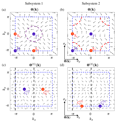
Here each block has the same dimension as . The diagonal blocks are copies of the static Hamiltonian, and the non-diagonal ones couple the th and th copies. The block-matrix form in Eq. (9) indicates that through exchanging energy with the system, the periodic driving shifts the copies of the static bands in steps of , and results in new band crossings (i.e., driving-induced BISs). Finite driving strength and SO coupling then open gaps on these BISs, rendering the Floquet bands Zhang2020 . Based on the above analysis, the Floquet system can be treated as a family of subsystems that are periodic in quasienergy, with each consisting of bands that are inverted on the corresponding BIS [see Fig. 1(a)]. Since driving-induced BISs are determined by () with SO couplings thereon reflecting higher-order effects Zhang2022 , we will hereinafter refer to the BIS (and also the subsystem) corresponding to a nonzero as the one of order . Due to the bulk-surface duality, the topology on the th BIS must be consistent with the bulk topology of the corresponding subsystem of the same order:
| (10) |
Here the superscript indicates the th BIS is of order and is the bulk topological invariant of the corresponding subsystem note_bulktopo . Together with Eq. (8), one can fully characterize Floquet topological phases once the topology of all subsystems is identified.
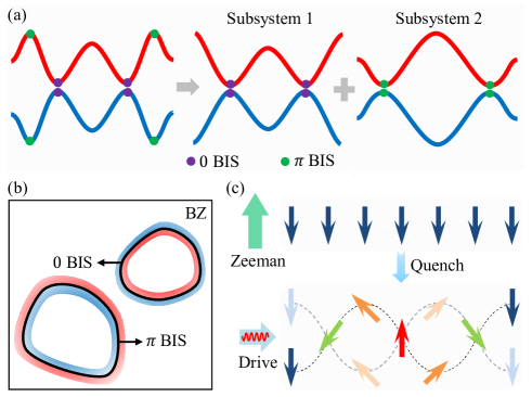
It should be noted that from the above picture, only the information in the immediate regions adjacent to and along BISs is reliable for defining effective Hamiltonians for subsystems [see the colored regions in Fig. 1(b)]. For example, when the driving takes a special form , the effective Hamiltonian for the subsystem of order can be obtained by analytic continuation of an effective Hamiltonian defined only on the corresponding BIS Zhang2022 , which reads
| (11) |
where , with being the Bessel function and . As a natural result, the characterization should also only use the data measured in the “regions of validity” to identify bulk topological invariants , which serves as one of the basic principles of our dynamical scheme.
We now present how to detect the bulk topology of subsystems by quench dynamics. We consider a quench along the axis and write . Here denotes the momentum-dependent part and represents a constant magnetization. The dynamics is induced by suddenly quenching a fully polarized trivial phase with to the target Floquet topological regime at [see Fig. 1(c)]. We employ stroboscopic time-averaged spin textures for characterization:
| (12) |
where , with the subscript outside the angle brackets denoting the quench axis. Here, is the density matrix of the initial state, which satisfies . Since with , we have
| (13) |
which indicates that the characterization can determine two different kinds of surfaces, i.e., those momenta where and , respectively. In particular, the surfaces where should appear in all the stroboscopic time-averaged spin textures, independent of the measurement axis . Based on this result, we introduce the concept of dynamical band-inversion surfaces,
| (14) |
which identify the surface in the deep-quench limit. Besides dBISs, one can also find other subspaces where stroboscopic time averages vanish. We denote
| (15) |
to characterize the surfaces .
Up to now, there are two special spin-polarization axes that have been mentioned: One is which defines the BIS and the other is the quench axis . Thus, the consideration of dynamical characterization should be divided into the following two cases: (i) The chosen quench axis is precisely the axis, i.e., ; and (ii) they are not the same, namely, .
Case (i). In this case, the measured dBISs correspond exactly to the BISs of the Floquet bands. According to the band structure or by observing how dBISs emerge one by one with the driving frequency Zhang2023 , one can determine which category each dBIS falls into, such as 0 or type and the order . Then, a dynamical spin-texture field can be defined to characterize the SO field, with
| (16) |
Here is the momentum perpendicular to dBISs and pointing from the region to , and is a normalization factor. It can be checked that on dBISs. The subsystem topology can be characterized by the winding of the dynamical field on the corresponding dBISs:
| (17) |
where denotes the dBISs that characterize the BISs of order .
Cases (ii). One needs first to rearrange the matrices into a new sequence which should also satisfy the trace property (2). Suppose (). The surfaces defined by Eq. (15) (rather than the dBISs) are factually the BISs of the Floquet bands, and can be divided into categories associated with different , denoted as . To characterize the subsystem topology correctly, one then needs to construct a spin texture for each subsystem from the measured result . For a given , the construction of the spin texture is as follows: The surfaces together with the dBISs cut the BZ into patches; the spin polarization of each whole patch ( or ) is determined by the measured value of in the adjacent region of located in this patch [i.e., the region of validity as sketched in Fig. 1(b)]. A dynamical field can then be defined for each subsystem, with the components given by Eq. (16) except that
| (18) |
The bulk topology of each subsystem is then characterized by the winding of the corresponding field on all dBISs:
| (19) |
For both cases, the winding numbers that characterize the topology of quasienergy gaps are obtained by
| (20) |
where is an integer.
Before proceeding, we would like to emphasize several points on dBISs: (i) Why do we define dBISs as Eq. (14)? The reason is that if we pick up any other axis but to define dBISs, we cannot construct a -component dynamical field to characterize the topology. From Eq. (13), we see for , which indicates that one can use the measurement to characterize the corresponding component . However, when , it becomes , which means the full information of cannot be derived from . Thus, to realize the dynamical characterization, the only choice is to use to define dBISs, and use other measurements to construct the dynamical field on dBISs. (ii) The fact that dBISs appear in all the spin textures can be understood as follows: The quench-induced spin oscillation at each corresponds to a spin precession, in which the momentum-linked spin rotates about the postquench vector field . The dBISs actually refer to the momenta where the spin state is perpendicular to its rotation axis. This naturally leads to the conclusion that on a dBIS, the time-averaged spin polarization is zero in any direction. (iii) dBISs are not the same as BISs, although they may refer to the same momentum subspace in case (i). While BISs are defined with respect to the (Floquet) band structure [see Eq. (3)], dBISs are defined with respect to dynamical measurements and used for the dynamical characterization by time-averaged spin textures [Eq. (14)]. For a Floquet system, the spin-polarization axis used to define BISs needs to be a special one that dominates the band dispersion. In comparison, the quench axis that determines dBISs can be any one in the present dynamical characterization scheme.
III.2 2D model
Now we use an experimentally feasible model to illustrate the scheme. We consider the 2D driven model taking the form of Eq. (1) with
| (21) |
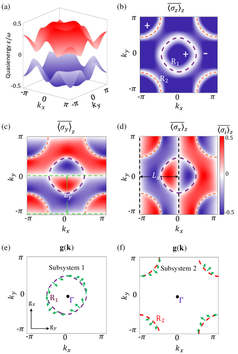
where are the Pauli matrices and depicts the 2D quantum anomalous Hall model that has been realized in optical Raman lattices Wu2016 ; Sun2018a ; Liang2023 . Here represents the spin-conserved (spin-flipped) hopping coefficient and denote the constant magnetization. The periodic drive can be achieved by modulating the bias magnetic field or the laser frequency Zhang2023 . For the static Hamiltonian , the bulk topology is simply determined by the Zeeman term (): the Chern number for and for . The applied drive can, however, largely modify the band structure, leading to a much richer Floquet topological phase diagram Zhang2023 . Figure 2(a) displays the quasienergy spectra of a phase with at , where both the BISs () are induced by the driving and correspond to with () and (), respectively [see Fig. 2(b)]. The result in Eq. (11) gives an expression of (), which describes subsystem 1 (2) corresponding to the driving-induced BIS ( BIS ). Note that in Fig. 2, the setting is comparable to the driving frequency , indicating that BISs should be defined with respect to the axis, for only can reflect all the band crossings in both the 0 gap and the gap. Otherwise, the topology of the gap cannot be characterized if we use to define BISs.
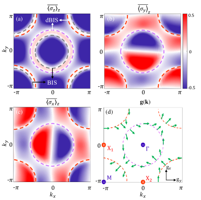
As described in Sec. III.1, the flexibility of the present characterization scheme allows us to consider different methods of quenching, which can benefit experimental measurements. Here we consider both of the aforementioned quench cases: (i) The quench axis is precisely the axis for this 2D driven model, and (ii) the quench is along another axis. For case (i), the quench is performed by suddenly varying from to at time , while setting . The periodic driving begins from as well [Fig. 1(c)]. We investigate the quench-induced spin dynamics and derive the stroboscopic time-averaged spin textures () based on Eq. (12). The results are shown in Figs. 2(b)-2(d). One can see that two ring-shaped structures [i.e., two dBISs as defined in Eq. (14)] emerge in all the spin textures, of which one () corresponds to a BIS and the other () identifies a BIS. According to Eq. (16), a dynamical spin-texture field is further constructed and is depicted with green arrows in Figs. 2(e) and 2(f). One can find that the dynamical field exhibits nonzero but opposite windings on the two rings note_winding , giving and . The Chern number of the Floquet bands is .
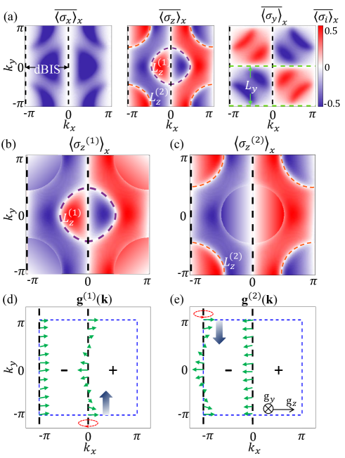
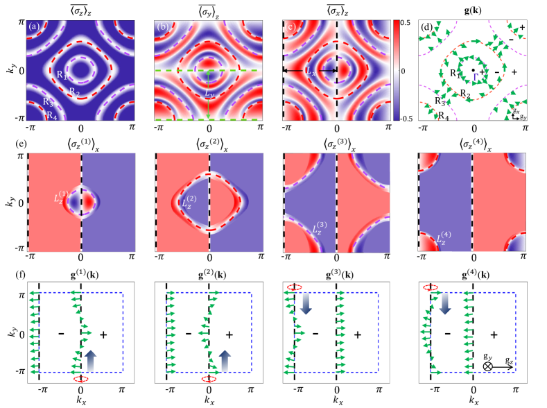
For case (ii), we quench the axis by changing from to , while setting and . The other steps are the same as in case (i). The stroboscopic time-averaged spin textures () are shown in Fig. 3(a). One sees that two line-shaped structures appear in all the spin textures, corresponding to two open dBISs at and , respectively. Other curves with vanishing spin polarization that only appear in () are denoted as (). Note that the curve () is in fact the BIS ( BIS). To characterize the subsystem topology, we need to construct a spin texture for each subsystem. The results are shown in Figs. 3(b) and 3(c). For each , the curves and dBISs cut the BZ into four patches; each patch is painted red or blue according to the spin polarization in the region of validity adjacent to [cf. Fig 1(b)]. Based on Eqs. (16) and (18), dynamical spin-texture fields can be constructed on the dBISs to characterize the two subsystems. One can see that despite a trivial pattern along the line (), the winding of the dynamical field [] on the other dBIS at () characterizes the topological invariant (). The results are the same as case (i), which confirms that the present dynamical characterization scheme is independent of the quench axis.
Despite the fact that only one anomalous topological phase is studied here, the dynamical characterization scheme can certainly be applied to other 2D Floquet topological phases. In Appendix B, we show a dynamical characterization of an unconventional topological phase called the anomalous Floquet valley-Hall phase Zhang2022 ; Zhang2023 .
III.3 3D model
We further apply our scheme to characterize a 3D driven model of the form in Eq. (1) with
| (22) | ||||
Here we denote and take , , and , where and are both Pauli matrices. The static Hamiltonian , having been simulated using solid-state spin systems Ji2020 ; Xin2020 , respects the chiral symmetry and describes 3D chiral topological phases including three regions: (I) with winding number ; (II) with ; and (III) with . In the presence of the driving , it can be checked that the corresponding Floquet Hamiltonian takes the form of Eq. (7), which maintains the same chiral symmetry and hosts anomalous chiral topological phases that can be identified by BIS characterization theory Zhang2022 .
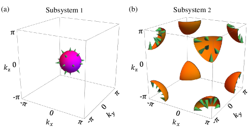
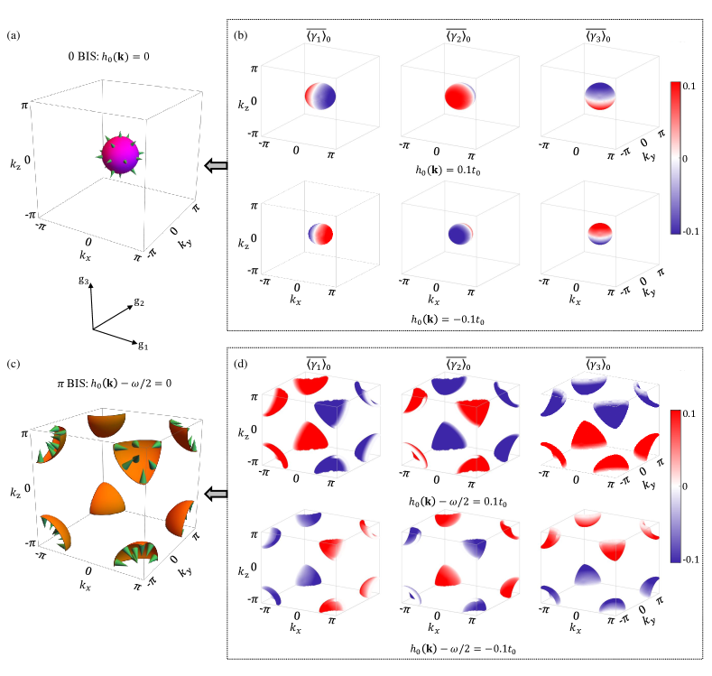
The dynamical characterization of the 3D driven model can be achieved by quenching [belonging to case (i)]. For post-quench parameters and , the Floquet topology of the 3D anomalous chiral topological phase is contributed from two static effective subsystems, one corresponding to the static BIS with [Fig. 4(a)] and the other to a driving-induced BIS with [Fig. 4(b)]. The dynamical spin-texture field on each surface can be derived from stroboscopic time-averaged spin textures (see Appendix C for details), the winding of which yields . We then have , which reveals the nontrivial topology within the two gaps, but indicates that the Floquet bands are topologically trivial.
The numerical results above demonstrate the feasibility of the present dynamical characterization scheme. Although only 2D and 3D models are examined, the characterization can easily be generalized to higher dimensions.
IV The viewpoint of topological charges
In this section, we adopt an alternative viewpoint to examine the dynamical characterization scheme. As in static systems Zhang2019a ; Yi2019 , the dynamical characterization of Floquet topological phases can also be achieved from the viewpoint of topological charges. Our starting point is still Eqs. (14) and (15) following the same quench protocol described in Sec. III.1. Also, two cases need to be considered.
For case (i) with , the dBISs defined in Eq. (14) characterize the BISs of the Floquet bands. We introduce dynamical charges that are located at the intersection points of all surfaces with :
| (23) |
Obviously, in this case, the dynamical charges are exactly the topological charges located at the nodes of the SO field . Since [see Eq. (13)], we define a dynamical spin-texture field , with its components given by
| (24) |
The charge value of the th dynamical charge is obtained by
| (25) |
The characterization of a subsystem of order reduces to the total dynamical charges enclosed by the corresponding dBISs:
| (26) |
where denotes the region surrounded by the corresponding dBISs with note_h0 . Here, denotes the -component of the effective Hamiltonian for the subsystem of order .
For case (ii) with , the matrices need to be rearranged. We also suppose () in the rearranged sequence, and denote by the surface that corresponds to the BIS of order . We identify the dynamical charges located at the intersection points :
| (27) |
Accordingly, we introduce the dynamical spin-texture field , where
| (28) |
and other components are given by Eq. (24). In this case, the dynamical charges do not correspond to the topological charges of the SO field. The topology of each subsystem is characterized by the corresponding dynamical charges enclosed by dBISs:
| (29) |
where denotes the region surrounded by dBISs with note_h0 , and the charge value is given by
| (30) |
Here we take the 2D driven model (21) as an example to illustrate the dynamical characterization via topological charges. The quench process, the chosen parameters, and the calculated stroboscopic time-averaged spin textures are all the same as those in Sec. III.2. We also consider the two quench cases. In case (i) with being quenched, the lines in Fig. 2(b) intersect at four points, identifying four distinct dynamical charges for both subsystems [see Figs. 5(a) and 5(b)]. The dynamical field is constructed from the spin textures according to Eq. (24), and determines the charge values. For subsystem 1 of order , only a single charge with at point is enclosed by the BIS [Fig. 5(a)], giving the bulk topological invariant . For subsystem 2 of order , three dynamical charges, one with at and two with at , are enclosed by the BIS [Fig. 5(b)]. The total charge value gives . In case (ii), the two subsystems have different dynamical charges [Figs. 5(c) and 5(d)]. Based on the spin textures in Fig. 3(a), two dynamical fields can be constructed, each of which characterizes the charges for the corresponding subsystem. We find that for subsystem 1 (2), the curves () and have two intersections marking two dynamical charges, and only the charge with () is enclosed by the two open dBISs, which yields (). One can see that in both cases, we have and , consistent with the characterization in Sec. III.2.
V Shallow Quenches
Our results above have shown that by quenching a fully polarized initial state, the induced quantum dynamics can characterize the topology of post-quench Floquet Hamiltonian . However, in systems such as ultracold atoms, only finite magnetization can be generated Yi2019 , so that one needs to consider the case of a shallow quench, i.e., the quench starts from an initial state that is incompletely polarized. It has been demonstrated for static systems that the dynamical bulk-surface correspondence (and thereby the dynamical characterization) is still valid for a shallow quench, since an incompletely polarized initial state can always be transformed to a fully polarized one by a local rotation Zhang2019b . Similar reasoning can be applied here. We shall show that the present dynamical characterization scheme for Floquet systems also works in the incompletely polarized case. Some details are given in Appendix D.
We assume a local rotation under which the rotated initial state becomes fully polarized. In the rotated frame, the Floquet Hamiltonian is now . Note that , where . After the rotation, the dynamical characterization becomes the one to characterize the topology of by a deep quench, and obviously it works. Since is local unitary, which is ensured by the fact that and are in the same trivial regime, the two Hamiltonians and must be topologically equivalent. This concludes our proof.
For illustration, we still consider the model described by Eq. (21). Here the quench process is realized by changing from a finite value in the trivial regime to the targeted value . We investigate the post-quench spin dynamics under the setting , with the stroboscopic time-averaged spin textures () being shown in Fig. 6(a)–6(c). One can see that two ring-shaped dBISs emerge in all the spin textures. The dBISs vary with the initial magnetization : When , they coincide with the BISs where ; when , the two dBISs deviate from the locations of BISs and move gradually towards each other. We see that as long as , each BIS must have its dynamical counterpart, and the emergent topology on dBISs yields a valid characterization of the postquench Floquet topological phase. As shown in Fig. 6(d), the winding of the dynamical field on dBISs and the total enclosed charges give the same Floquet topological invariants and as the deep-quench cases discussed in former sections.
VI Discussion and Conclusions
We have presented a general and feasible dynamical characterization scheme for a class of generic periodically driven systems classified by -valued topological invariants. The scope of application of our proposed dynamical scheme is detailed in Appendix A. The present scheme is based on the BIS characterization theory, which reduces the characterization of the bulk topology to a sum of contributions of lower-dimensional topology in local momentum subspaces called BISs. Such a theory has two major advantages: (i) The local topology on BISs can be directly and precisely measured by quench dynamics, which has been experimentally demonstrated in several artificial quantum simulators Yi2019 ; Wang2019 ; Ji2020 ; Xin2020 ; Niu2021 ; Zhang2023 . (ii) The classification by local topological structures enables the realization and detection of novel Floquet topological phases beyond the conventional characterization Zhang2022 ; Zhang2023 . It has been shown that a particular local topological structure formed in each BIS can uniquely correspond to a gapless edge mode, rendering the BIS-boundary correspondence Zhang2022 . Hence, a dynamical scheme based on the BIS characterization potentially has wider applicability. An example is given in Appendix B to showcase an unconventional topological phase and its dynamical characterization.
Compared with the previous work in Ref. Zhang2020 , the present dynamical scheme is more flexible in performing quenches. The previous work directly employs the dynamical patterns emerging on BISs to characterize the bulk topology, which depends on how we define the BISs and thus restricts the quench axis. In comparison, the present scheme introduces effective static Hamiltonians to replace the role of BISs; these Hamiltonians have the bulk topology in one-to-one correspondence to the subdimensional topology defined on BISs. Characterizing a static bulk Hamiltonian can be achieved by a quench along an arbitrary spin-polarization axis Zhang2018 .
The present scheme also works under nonideal conditions. Two aspects are discussed here: (i) Although stroboscopic time-averaged spin textures in Eq. (12) are defined over an infinite interval, quench dynamics up to only several oscillation periods , where denotes the local energy gap of the Floquet bands, can usually provide sufficient information for topological characterization Yi2019 ; Zhang2023 . This indicates that the dynamical measurement is, to a certain extent, robust against thermal effects. (ii) As already discussed in Sec. V, the proposed dynamical scheme can also employ shallow quenches, which loosens the restriction on the preparation of the initial state and has practical benefits for experimental realization. We have proved that as long as the initial state is in the same trivial regime as the fully polarized state, the present scheme always yields a valid dynamical characterization.
Our dynamical characterization theory can also employ a set of quenches with respect to all spin-quantization axes. The result in Eq. (13) shows an important duality that measuring the th spin component after quenching the th spin-quantization axis precisely equals to measuring the th spin component after quenching the th axis. Hence, one can easily check that all the stroboscopic time-averaged spin textures that are required for characterization can alternatively be obtained by measuring a single component after a set of quenches along all spin-quantization axes Zhang2019a ; Zhang2019b . However, it should also be noted that whether or not the scheme using a set of shallow quenches can yield a valid characterization of Floquet topological phases is not a straightforward question and deserves further investigation.
In summary, our work provides a multiple-subsystem approach for characterizing Floquet topological phases by quantum quenches. The present scheme has high flexibility and feasibility in practical applications and can be immediately applied in ultracold atoms or other quantum simulators.
Note added. Recently, we noted that a dynamical characterization theory has been developed for Floquet topological phases based on the concept of higher-order BISs Zhanglin2023 .
Acknowledgements
This work was supported by the National Natural Science Foundation of China (Grants No. 12204187), the Innovation Program for Quantum Science and Technology (Grant No. 2021ZD0302000), and a startup grant of Huazhong University of Science and Technology (Grant No. 3004012204).
Appendix A The scope of application of our dynamical characterization scheme
In this appendix, we specify what kinds of Floquet topological phases our dynamic characterization scheme can apply to. As shown in Eq. (1), we consider a class of periodically driven systems realized by applying a periodic drive on top of a -dimensional (D) time-independent band structure. For the latter, we focus on generic gapped topological phases classified by integers in the AZ symmetry classes AZ1997 ; Schnyder2008 ; Kitaev2009 ; Chiu2016 . We shall elaborate on this as follows.
First, the basic Hamiltonian for the static system takes the form
| (31) |
where the matrices obey the anticommutation relations, and are of dimensionality (or ) if is even (or odd), involving the minimal bands to open a topological gap. The matrices can generally be constructed as the tensor product of the Pauli matrices, e.g., in the 3D Hamiltonian (22). In one and two dimensions, the Clifford matrices simply reduce to the Pauli matrices [cf. Eq. (21)]. Generally, these topological phases can be topological insulators or superconductors characterized by the winding number (Chern number) in odd (even) dimensions, including classes AIII, BDI, and CII in one dimension, classes A, D, and C in two dimensions, classes AIII, DIII, and CI in three dimensions, and so on. In odd dimensions, these topological phases require the protection of the chiral symmetry . Here, the winding or Chern number characterizes the wrapping number of the map from a D torus to the D spherical surface . For such D topological phases described by Eq. (31), the bulk topology can be characterized by a D invariant defined on BISs, rendering the bulk-surface duality Zhang2018 ; Zhang2019a ; Zhang2019b .
Second, for the total Hamiltonian, we consider the topology of the Floquet Hamiltonian . Due to the classification of the static Hamiltonian, the resulting Floquet topological phases can also be classified by -valued invariants in the ten symmetry classes, as long as the total Hamiltonian respects the required nonspatial symmetries Roy2017 ; Yao2017 . Besides, they can also be unconventional topological phases beyond the ten-way classification Zhang2022 (see Appendix B for an example). When the periodic driving takes the form with , the effective Hamiltonian also takes the basic Dirac-type form shown in Eq. (7). Hence there exist two inequivalent Floquet gaps, named the 0 gap and the gap, respectively, and each gap is characterized by a invariant. A generalized bulk-surface duality has been established Zhang2020 : The gap topology can be characterized by a D invariant defined on the BISs associated with the corresponding gap.
Third, our characterization theory can be generalized to generic multiband systems, for which we assume that each (quasi)energy gap is opened through a group of bands (the minimal requirement). At each , the multiband Hamiltonian can be transformed into a block-diagonal form Zhang2018 . One can see that only those blocks involving crossing bands have nontrivial contribution to the topology. The topology of the bulk bands can then be reduced to topological invariants defined on the corresponding BISs of each block. The contribution of a BIS is effectively determined by a basic Hamiltonian taking the form in Eq. (31). For example, in a 2D three-band system, any two bands that have a band crossing can be locally described by a two-band effective Hamiltonian. A topological invariant can then be defined on each BIS, which characterizes the bulk topology of the effective Hamiltonian and has a contribution to the Chern numbers of the two involved bands. Such a generalization applies to both static and Floquet systems. The only difference is that for a Floquet system, one also needs to consider the band crossings resulting from the periodicity of the quasienergy.
Appendix B Dynamical characterization of the anomalous Floquet valley-Hall phase
In this appendix, we apply the present dynamical characterization scheme to more “unconventional” topological phases. As demonstrated in Ref. Zhang2022 , the concept of BIS provides a systematic way to realize various topological phases by Floquet engineering local topological structures. In particular, when two BISs with opposite topology emerge in the same quasienergy gap, the system may exhibit a topological phase that cannot be classified by conventional topological invariants, e.g., the winding numbers and the Chern number, defined for the global topology of the bulk. A typical example is the anomalous Floquet valley-Hall phase Zhang2022 ; Zhang2023 .
For the 2D driven model described by Eq. (21), the anomalous Floquet valley-Hall phase is marked by four ring-shaped BISs in the first BZ [see Fig. 7(a)]: Two correspond to BISs () and two are BISs (); they are all induced by periodic driving for the chosen parameters. Here for clarity of the results, we set an initial driving phase in the driving so that , which does not alter the Floquet topology Zhang2020 . The two types of BISs (two 0 BISs or two BISs) exhibit the same configuration: One BIS (e.g., ) surrounds the point, and the other (e.g., ) surrounds . The dynamical characterization shows that such a configuration results in two opposite contributions to the topological invariant . According to the stroboscopic time-averaged spin textures () in Fig. 7(a)–7(c), the dynamical field can be constructed [Fig. 7(d)], the winding of which on each dBIS gives (for ) and (for ). Hence, we have , , and the Chern number of the Floquet bands . These topological invariants defined to characterize the global bulk topology are all equal to zero. However, it has been proved that this phase features stable counterpropagating edge states in both quasienergy gaps, and thus transcends the conventional classification Zhang2022 .
The characterization can also be performed by quenching the axis. By following the same procedure as in Fig. 3, we construct four spin textures from the measurement [Fig. 7(e)], each obtained by extending the data measured in the adjacent region of the corresponding BIS (labeled by ). Accordingly, the dynamical fields are depicted on the two open dBISs [Fig. 7(f)], whose winding characterizes the subsystem topology. One can easily check that the characterization yields the same results as above: and .
Appendix C Dynamical characterization of 3D topological phases
In this appendix, we present the details of numerical calculations of the 3D model in Sec. III.3. Here we perform a quench in the axis, while the characterization can also be achieved by other quenches. As described in the main text, the static Hamiltonian has three topological phase regions distinguished by . The phase displayed in Fig. 4 is realized by applying a periodic drive to the phase in region (I).
Similar to the 2D driven model, we detect the 3D Floquet topological phases by quenching an initial fully polarized state and deriving stroboscopic time-averaged spin textures () from quench dynamics. For the chosen post-quench parameters, two dBISs can be identified by for all (see Fig. 8). Since the quench axis is the one that defines the BIS with , the two spherical-like surfaces in Fig. 8 (a) and 8(c) are in fact the BISs of the Floquet bands: One is a 0 BIS with [Fig. 8(a)] and the other is a BIS with [Fig. 8(b)]. Accordingly, the whole Floquet system is disassembled into two static subsystems, each corresponding to one BIS.
According to Eq. (16), the dynamical spin-texture field is defined by the gradient of perpendicular to the dBISs. Here we show the calculated spin textures on the closed surfaces slightly inside and outside the BISs, respectively [Fig. 8(b) and 8(d)]. The direction of the dynamical field on each BIS can be determined by the subtraction of on the neighboring equal-energy surfaces. From the winding of , one can obtain the bulk topological invariants for subsystems , which gives , and the winding number of the Floquet bands .
Appendix D Some details on shallow quenches
Here we give more details on the proof of the shallow-quench method. Since , with , we have
| (32) |
which yields in a deep-quench case where . When , dBISs defined by Eq. (14) are exactly the BISs. However, for a shallow quench, they are in general not equal [see Fig. 6(a)]. The definition in Eq. (14) in fact gives
| (33) |
Now we examine the dynamical characterization. For shallow quenches, the direction is defined to be perpendicular to the contours of the dBISs, i.e., . Suppose that the spin textures are all linear in when approaching the dBISs. The directional derivative on dBISs then reads
| (34) |
We then have . As argued in Sec. V, as long as the incompletely polarized initial state can be connected to the fully polarized one via a local unitary rotation, the topological patterns on dBISs should remain the same. This leads to the conclusion that the dynamical characterization by shallow quenches yields the same result as in the deep-quench case.
References
- (1) M. Z. Hasan and C. L. Kane, Colloquium: Topological insulators, Rev. Mod. Phys. 82, 3045 (2010).
- (2) X.-L. Qi and S.-C. Zhang, Topological insulators and superconductors, Rev. Mod. Phys. 83, 1057 (2011).
- (3) M. Sato and Y. Ando, Topological superconductors: a review, Rep. Prog. Phys. 80, 076501 (2017).
- (4) C. Fang, H. Weng, X. Dai, and Z. Fang, Topological nodal line semimetals, Chinese Phys. B, 25, 117106 (2016).
- (5) D.-W. Zhang, Y.-Q. Zhu, Y. X. Zhao, H. Yan, S.-L. Zhu, Topological quantum matter with cold atoms, Adv. Phys. 67, 253 (2018).
- (6) N. R. Cooper, J. Dalibard, and I. B. Spielman, Topological bands for ultracold atoms, Rev. Mod. Phys. 91, 015005 (2019).
- (7) F. Schäfer, T. Fukuhara, S. Sugawa, Y. Takasu, and Y. Takahashi, Tools for quantum simulation with ultracold atoms in optical lattices, Nat. Rev. Phys. 2, 411 (2020).
- (8) M. Atala, M. Aidelsburger, J. T. Barreiro, D. Abanin, T. Kitagawa, E. Demler, and I. Bloch, Direct measurement of the Zak phase in topological Bloch bands, Nat. Phys. 9, 795 (2013).
- (9) B. Song, L. Zhang, C. He, T. F. J. Poon, E. Hajiyev, S. Zhang, X.-J. Liu, and G.-B. Jo, Observation of symmetry-protected topological band with ultracold fermions, Sci. Adv. 4, eaao4748 (2018).
- (10) M. Aidelsburger, M. Atala, M. Lohse, J. T. Barreiro, B. Paredes, and I. Bloch, Realization of the Hofstadter Hamiltonian with Ultracold Atoms in Optical Lattices, Phys. Rev. Lett. 111, 185301 (2013).
- (11) H. Miyake, G. A. Siviloglou, C. J. Kennedy, W. C. Burton, and W. Ketterle, Realizing the Harper Hamiltonian with LaserAssisted Tunneling in Optical Lattices, Phys. Rev. Lett. 111, 185302 (2013).
- (12) G. Jotzu, M. Messer, R. Desbuquois, M. Lebrat, T. Uehlinger, D. Greif, and T. Esslinger, Experimental realization of the topological Haldane model with ultracold fermions, Nature (London) 515, 237 (2014).
- (13) M. Aidelsburger, M. Lohse, C. Schweizer, M. Atala, J. T. Barreiro, S. Nascimbène, N. R. Cooper, I. Bloch, and N. Goldman, Measuring the Chern number of Hofstadter bands with ultracold bosonic atoms, Nat. Phys. 11, 162 (2015).
- (14) Z. Wu, L. Zhang, W. Sun, X. Xu, B. Wang, S. Ji, Y. Deng, S. Chen, X. Liu, and J.-W. Pan, Realization of two-dimensional spin-orbit coupling for Bose-Einstein condensates, Science, 354, 83-88, (2016).
- (15) W. Sun, B.-Z. Wang, X.-T. Xu, C.-R. Yi, L. Zhang, Z. Wu, Y. Deng, X.-J. Liu, S. Chen, and J.-W. Pan, Highly Controllable and Robust 2D Spin-Orbit Coupling for Quantum Gases, Phys. Rev. Lett. 121, 150401 (2018).
- (16) M.-C. Liang, Y.-D. Wei, L. Zhang, X.-J. Wang, H. Zhang, W.-W. Wang, W. Qi, X.-J. Liu, and X. Zhang, Realization of Qi-Wu-Zhang model in spin-orbit-coupled ultracold fermions, Phys. Rev. Research 5, L012006 (2023).
- (17) B. Song, C. He, S. Niu, L. Zhang, Z. Ren, X.-J. Liu, and G.-B. Jo, Observation of nodal-line semimetal with ultracold fermions in an optical lattice, Nat. Phys. 15, 911 (2019).
- (18) Z. Wang, X. Cheng, B. Wang, J. Zhang, Y. Lu, C. Yi, S. Niu, Y. Deng, X. Liu, S. Chen, and J.-W. Pan, Realization of an ideal Weyl semimetal band in a quantum gas with 3D spin-orbit coupling, Science, 372, 271. (2021).
- (19) X.-J. Liu, Z.-X. Liu, and M. Cheng, Manipulating Topological Edge Spins in a One-Dimensional Optical Lattice, Phys. Rev. Lett. 110, 076401 (2013).
- (20) X.-J. Liu, K. T. Law, and T. K. Ng, Realization of 2D Spin-Orbit Interaction and Exotic Topological Orders in Cold Atoms, Phys. Rev. Lett. 112, 086401 (2014).
- (21) X. Zhou, J.-S. Pan, Z.-X. Liu, W. Zhang, W. Yi, G. Chen, and S. Jia, Symmetry-Protected Topological States for Interacting Fermions in Alkaline-Earth-Like Atoms, Phys. Rev. Lett. 119, 185701 (2017).
- (22) B.-Z. Wang, Y.-H. Lu, W. Sun, S. Chen, Y. Deng, and X.-J. Liu, Dirac-, Rashba-, and Weyl-type spin-orbit couplings: Toward experimental realization in ultracold atoms, Phys. Rev. A 97, 011605(R) (2018).
- (23) Y.-H. Lu, B.-Z. Wang, X.-J. Liu, Ideal Weyl semimetal with 3D spin-orbit coupled ultracold quantum gas, Sci. Bull. 65, 2080 (2020).
- (24) Bei-Bei Wang, Jia-Hui Zhang, Chuanjia Shan, Feng Mei and Suotang Jia, Topological nodal chains in optical lattices, Phys. Rev. A 103, 033316 (2021).
- (25) L. Ziegler, E. Tirrito, M. Lewenstein, S. Hands, and A. Bermudez, Correlated Chern insulators in two-dimensional Raman lattices: A cold-atom regularization of strongly coupled four-Fermi field theories, Phys. Rev. Research 4, L042012 (2022).
- (26) A. Eckardt, Colloquium: Atomic quantum gases in periodically driven optical lattices, Rev. Mod. Phys. 89, 011004 (2017).
- (27) M. S. Rudner and N. H. Lindner, Band structure engineering and non-equilibrium dynamics in Floquet topological insulators. Nat. Rev. Phys. 2, 229 (2020).
- (28) F. Harper, R. Roy, M. S. Rudner, and S. L. Sondhi, Topology and Broken Symmetry in Floquet Systems, Annu. Rev. Condens. Matter Phys. 11, 345 (2020).
- (29) C. Weitenberg and J. Simonet, Tailoring quantum gases by Floquet engineering, Nat. Phys. 17, 1342 (2021).
- (30) M. S. Rudner, N. H. Lindner, E. Berg, and M. Levin, Anomalous Edge States and the Bulk-Edge Correspondence for Periodically Driven Two-Dimensional Systems, Phys. Rev. X 3, 031005 (2013).
- (31) N. Goldman and J. Dalibard, Periodically Driven Quantum Systems: Effective Hamiltonians and Engineered Gauge Fields, Phys. Rev. X 4, 031027 (2014).
- (32) M. Bukov, L. D’Alessio, and A. Polkovnikov, Universal high-frequency behavior of periodically driven systems: from dynamical stabilization to Floquet engineering, Adv. Phys. 64, 139 (2015).
- (33) B. Höckendorf, A. Alvermann, and H. Fehske, Universal driving protocol for symmetry-protected Floquet topological phases, Phys. Rev. B 99, 245102 (2019).
- (34) H. Liu, T.-S. Xiong, W. Zhang, and J.-H. An, Floquet engineering of exotic topological phases in systems of cold atoms, Phys. Rev. A 100, 023622 (2019).
- (35) Y. Peng and G. Refael, Floquet Second-Order Topological Insulators from Nonsymmorphic Space-Time Symmetries, Phys. Rev. Lett. 123, 016806 (2019).
- (36) H. Hu, B. Huang, E. Zhao, and W. V. Liu, Dynamical Singularities of Floquet Higher-Order Topological Insulators, Phys. Rev. Lett. 124, 057001 (2020).
- (37) B. Huang and W. V. Liu, Floquet Higher-order topological insulators with anomalous dynamical polarization, Phys. Rev. Lett. 124, 216601 (2020).
- (38) M. Jangjan, L. E. F. F. Torres, and M. V. Hosseini, Floquet topological phase transitions in a periodically quenched dimer, Phys. Rev. B 106, 224306 (2022).
- (39) R.-J. Slager, A. Bouhon, and F. N. Ünal, Floquet multi-gap topology: Non-Abelian braiding and anomalous Dirac string phase, arXiv: 2208.12824.
- (40) T. Li and H. Hu, Floquet non-Abelian topological insulator and multifold bulk-edge correspondence, Nat. Commun. 14, 6418 (2023).
- (41) K. Wintersperger, C. Braun, F. N. Ünal, A. Eckardt, M. D. Liberto, N. Goldman, I. Bloch and M. Aidelsburger, Realization of an anomalous Floquet topological system with ultracold atoms, Nat. Phys. 16, 1058 (2020).
- (42) T. Kitagawa, E. Berg, M. Rudner, and E. Demler, Topological characterization of periodically driven quantum systems, Phys. Rev. B 82, 235114 (2010).
- (43) F. Nathan and M. S. Rudner, Topological singularities and the general classification of Floquet-Bloch systems, New J. Phys. 17, 125014 (2015).
- (44) D. Carpentier, P. Delplace, M. Fruchart, and K. Gawedzki, Topological Index for Periodically Driven Time-Reversal Invariant 2D Systems, Phys. Rev. Lett. 114, 106806 (2015).
- (45) M. Fruchart, Complex classes of periodically driven topological lattice systems, Phys. Rev. B 93, 115429 (2016).
- (46) R. Roy and F. Harper, Periodic table for Floquet topological insulators, Phys. Rev. B 96, 155118 (2017).
- (47) S. Yao, Z. Yan, and Z. Wang, Topological invariants of Floquet systems: General formulation, special properties, and Floquet topological defects, Phys. Rev. B 96, 195303 (2017).
- (48) T. Morimoto, H. C. Po, and A. Vishwanath Floquet topological phases protected by time glide symmetry, Phys. Rev. B 95, 195155 (2017).
- (49) F. N. Ünal, A. Eckardt, and R.-J. Slager, Hopf characterization of two-dimensional Floquet topological insulators, Phys. Rev. Research 1, 022003(R) (2019).
- (50) L. Zhang, L. Zhang, and X.-J. Liu, Unified Theory to Characterize Floquet Topological Phases by Quench Dynamics, Phys. Rev. Lett. 125, 183001 (2020).
- (51) L. Zhang and X.-J. Liu, Unconventional Floquet Topological Phases from Quantum Engineering of Band-Inversion Surfaces, PRX Quantum 3, 040312 (2022).
- (52) J.-Y. Zhang, C.-R. Yi, L. Zhang, R.-H. Jiao, K.-Y. Shi, H. Yuan, W. Zhang, X.-J. Liu, S. Chen, and J.-W. Pan, Tuning Anomalous Floquet Topological Bands with Ultracold Atoms, Phys. Rev. Lett. 130, 043201 (2023).
- (53) L. Zhang, L. Zhang, S. Niu, and X.-J. Liu, Dynamical classification of topological quantum phases, Sci. Bull. 63, 1385 (2018).
- (54) L. Zhang, L. Zhang, and X.-J. Liu, Dynamical detection of topological charges, Phys. Rev. A 99, 053606 (2019).
- (55) L. Zhang, L. Zhang, and X.-J. Liu, Characterizing topological phases by quantum quenches: A general theory, Phys. Rev. A 100, 063624 (2019).
- (56) H. Hu and E. Zhao, Topological Invariants for Quantum Quench Dynamics from Unitary Evolution, Phys. Rev. Lett. 124, 160402 (2020).
- (57) J. Ye and F. Li, Emergent topology under slow nonadiabatic quantum dynamics, Phys. Rev. A 102, 042209 (2020).
- (58) X.-L. Yu, W. Ji, L. Zhang, Y. Wang, J. Wu, and X.-J. Liu, Quantum Dynamical Characterization and Simulation of Topological Phases With High-Order Band Inversion Surfaces, PRX Quantum 2, 020320 (2021).
- (59) W. Jia, L. Zhang, L. Zhang, and X.-J. Liu, Dynamically characterizing topological phases by high-order topological charges Phys. Rev. A 103, 052213 (2021).
- (60) L. Li, W. Zhu, and J. Gong, Direct dynamical characterization of higher-order topological phases with nested band inversion surfaces, Sci. Bull. 66, 1502 (2021).
- (61) P. Fang, Y.-X. Wang, and F. Li, Generic theory of characterizing topological phases under quantum slow dynamics, Phys. Rev. A 106, 022219 (2022).
- (62) P. He, Y.-Q. Zhu, J.-T. Wang, and S.-L. Zhu, Quantum quenches in a pseudo-Hermitian Chern insulator, Phys. Rev. A 107, 012219 (2023).
- (63) T. Langen, R. Geiger, and J. Schmiedmayer, Ultracold Atoms Out of Equilibrium, Annu. Rev. Condens. Matter Phys. 6, 201 (2015).
- (64) M. D. Caio, N. R. Cooper, and M. J. Bhaseen, Quantum Quenches in Chern Insulators, Phys. Rev. Lett. 115, 236403 (2015).
- (65) N. Fläschner, B. S. Rem, M. Tarnowski, D. Vogel, D.-S. Lühmann, K. Sengstock, and C. Weitenberg, Experimental reconstruction of the Berry curvature in a Floquet Bloch band, Science 352, 1091 (2016).
- (66) C. Wang, P. Zhang, X. Chen, J. Yu, and H. Zhai, Scheme to Measure the Topological Number of a Chern Insulator from Quench Dynamics, Phys. Rev. Lett. 118, 185701 (2017).
- (67) N. Fläschner, D. Vogel, M. Tarnowski, B. S. Rem, D.-S. Lühmann, M. Heyl, J. C. Budich, L. Mathey, K. Sengstock, and C. Weitenberg, Observation of dynamical vortices after quenches in a system with topology, Nat. Phys. 14, 265 (2018).
- (68) M. Tarnowski, F. N. Ünal, N. Flächner, B. S. Rem, A. Eckardt, K. Sengstock, and C. Weitenberg, Characterizing topology by dynamics: Chern number from linking number, Nat. Commun. 10, 1728 (2019).
- (69) W. Sun, C.-R. Yi, B.-Z. Wang, W.-W. Zhang, B. C. Sanders, X.-T. Xu, Z.-Y. Wang, J. Schmiedmayer, Y. Deng, X.-J. Liu, S. Chen, and J.-W. Pan, Uncover Topology by Quantum Quench Dynamics, Phys. Rev. Lett. 121, 250403 (2018).
- (70) C.-R. Yi, L. Zhang, L. Zhang, R.-H. Jiao, X.-C. Cheng, Z.-Y. Wang, X.-T. Xu, W. Sun, X.-J. Liu, S. Chen, and J.- W. Pan, Observing Topological Charges and Dynamical Bulk-Surface Correspondence With Ultracold Atoms, Phys. Rev. Lett. 123, 190603 (2019).
- (71) F. N. Ünal, A. Bouhon, and R.-J. Slager, Topological Euler Class as a Dynamical Observable in Optical Lattices, Phys. Rev. Lett. 125, 053601 (2020).
- (72) Y. Wang, W. Ji, Z. Chai, Y. Guo, M. Wang, X. Ye, P. Yu, L. Zhang, X. Qin, P. Wang, F. Shi, X. Rong, D. Lu, X.-J. Liu, and J. Du, Experimental observation of dynamical bulk-surface correspondence for topological phases, Phys. Rev. A 100, 052328 (2019).
- (73) W. Ji, L. Zhang, M. Wang, L. Zhang, Y. Guo, Z. Chai, X. Rong, F. Shi, X.-J. Liu, Y. Wang, and J. Du, Quantum Simulation for Three-Dimensional Chiral Topological Insulator, Phys. Rev. Lett. 125, 020504 (2020).
- (74) T. Xin, Y. Li, Y. Fan, X. Zhu, Y. Zhang, X. Nie, J. Li, Q. Liu, and D. Lu, Quantum Phases of Three-Dimensional Chiral Topological Insulators on a Spin Quantum Simulator, Phys. Rev. Lett. 125, 090502 (2020).
- (75) J. Niu, T. Yan, Y. Zhou, Z. Tao, X. Li, W. Liu, L. Zhang, H. Jia, S. Liu, Z. Yan, Y. Chen, D. Yu, Simulation of higher-order topological phases and related topological phase transitions in a superconducting qubit, Sci. Bull. 66, 1168 (2021).
- (76) A. Altland and M. R. Zirnbauer, Nonstandard symmetry classes in mesoscopic normal-superconducting hybrid structures, Phys. Rev. B 55, 1142 (1997).
- (77) A. P. Schnyder, S. Ryu, A. Furusaki, and A. W. W. Ludwig, Classification of topological insulators and superconductors in three spatial dimensions, Phys. Rev. B 78, 195125 (2008).
- (78) A. Kitaev, Periodic table for topological insulators and superconductors, AIP Conference Proceedings 1134, 22 (2009).
- (79) C.-K. Chiu, J. C. Y. Teo, A. P. Schnyder, and S. Ryu, Classification of topological quantum matter with symmetries, Rev. Mod. Phys. 88, 035005 (2016).
- (80) A. Eckardt and E. Anisimovas, High-frequency approximation for periodically driven quantum systems from a Floquet-space perspective, New J. Phys. 17, 093039 (2015).
- (81) According to Eq. (8), topological invariants should be defined with respect to the Floquet bands below the 0 gap, i.e., to characterize the winding of spin-orbit coupling in the lower bands of BISs, which are also the upper bands of BISs due to the periodicity of the quasienergy. Therefore, based on Eq. (10), the bulk topological invariant should be defined to characterize the lower bands of the corresponding subsystem if is even but to characterize the upper bands if is odd. In our dynamical scheme, we indeed determine in this way even without particularly mentioning it. One can certainly define all in the same manner, which does not change the final result.
- (82) Note that the winding orientation should be identified with respect to the same reference point, e.g., the point. When tracing out the ring in an anticlockwise direction around , one can find that the dynamical field winds along the dBIS in a clockwise direction, indicating the associated topological number .
- (83) Here, the requirement is to ensure a unified classification of all subsystems, meanwhile being consistent with the definition of for different note_bulktopo . For example, in Fig. 5(a) and 5(b), refers to the region containing the point for both subsystems.
- (84) L. Zhang, Dynamical characterization of Floquet topological phases via quantum quenches, arXiv:2311.00114.