XLuminA:
An Auto-differentiating Discovery Framework for Super-Resolution Microscopy

Abstract

Driven by human ingenuity and creativity, the discovery of super-resolution techniques, which circumvent the classical diffraction limit of light, represent a leap in optical microscopy. However, the vast space encompassing all possible experimental configurations suggests that some powerful concepts and techniques might have not been discovered yet, and might never be with a human-driven direct design approach. Thus, AI-based exploration techniques could provide enormous benefit, by exploring this space in a fast, unbiased way. We introduce XLuminA, an original computational framework written in JAX, which offers enhanced computational speed enabled by its accelerated linear algebra compiler (XLA), just-in-time compilation, and its seamlessly integrated automatic vectorization, auto-differentiation capabilities and GPU compatibility. Remarkably, XLuminA demonstrates a computational speed-up factor of $\times$80 with respect to well-established light propagation algorithms. We showcase XLuminA’s potential by re-discovering three foundational experiments in advanced microscopy. Ultimately, XLuminA identified a novel experimental blueprint featuring sub-diffraction imaging capabilities.

I Introduction

The space of all possible experimental optical configurations is enormous. For example, if we consider experiments that consist of just 10 optical elements, chosen from 5 different components (such as lasers, lenses, phase shifters, beam splitters and cameras), we already get 10 million possible discrete arrangements. The experimental topology (i.e., how the elements are arranged) will further increase this number greatly. Finally, each of these optical components can have tunable parameters (such as lenses’ focal lengths, laser power or splitting ratios of beam splitters) which lead to additional high-dimensional continuous parameter space for each of the previously mentioned discrete possibilities. This vast search space contains all experimental designs possible, including those with exceptional properties. So far, researchers have been exploring this space of possibilities guided by experience, intuition and creativity – and have uncovered countless exciting experimental configurations and technologies. But due to the complexity of this space, it might be that some powerful concepts and techniques have not been discovered so far, and might never be with a human-driven direct design approach. This is where AI-based exploration techniques could provide enormous benefit, by exploring the space in a fast, unbiased way [1, 2].

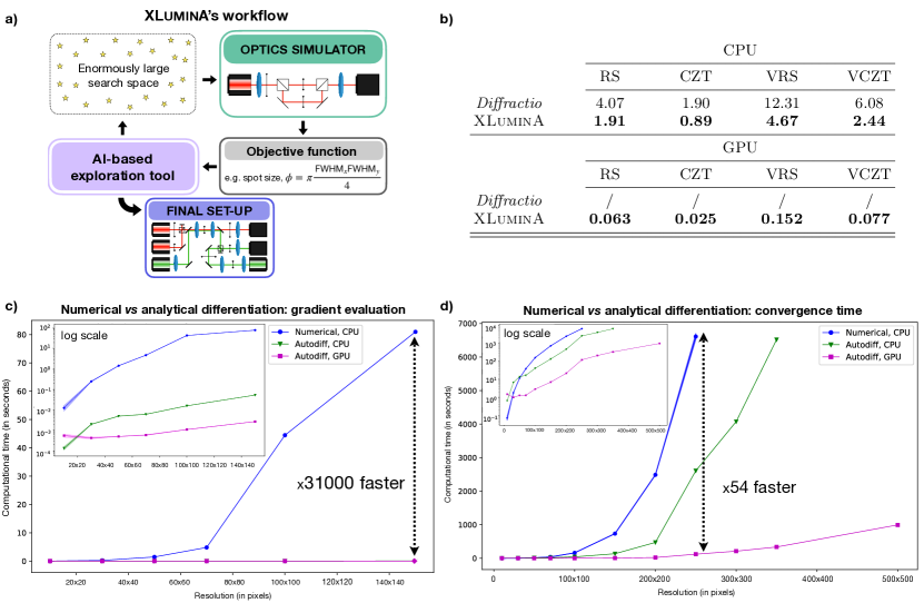
Figure 1: Overview and performance of XLuminA. (a) Software’s workflow, demonstrating the integrated feedback between the AI discovery tool and the optics simulator. Stars depict experimental blueprints with exceptional and useful properties. We start by feeding the system an initial random set of optical parameters, which shape the hardware design on a virtual optical table. The performance of the virtual experiment is computed by the simulator, which leads to detected light (e.g., captured images at the camera). From those simulated outputs, the objective function (for instance, the spot size), is computed. To improve the metric of the cost function, the optimizer adjusts the optical parameters in the initial virtual setup and the cycle is repeated. The whole process is a back-and-forth between the simulator and the optimizer, refining the setup until a convergence is observed. (b) Average execution time (in seconds) over 100 runs, within a resolution of $2048\times 2048$ pixels, for scalar and vectorial field propagation using Rayleigh-Sommerfeld (RS, VRS) and Chirped z-transform (CZT, VCZT) algorithms in Diffractio and XLuminA. Times for XLuminA correspond to runs with pre-compiled jitted functions. Our methods demonstrate enhanced computational speeds for simulating light diffraction and propagation: a factor of $\times$2 for RS and CZT and about $\times$2.5 for VRS and VCZT using the CPU. With GPU utilization, the speed increases up to two orders of magnitude with factors of $\times$64 for RS, $\times$76 for CZT, $\times$80 for VRS and $\times$78 for VCZT. The single run data is depicted in Extended Data Fig. 1. (c) Average time (in seconds) over 5 runs for a single gradient evaluation using numerical (blue dots) and autodiff methods (green triangles for CPU and magenta squares for GPU) on XLuminA’s optical simulator for different resolutions. The use of autodiff improves the gradient evaluation time by a factor of $\times$31 thousand in the GPU and a factor of $\times$1500 on the CPU for resolutions of $140\times 140$. The superior efficiency of autodiff over traditional numerical methods allows for highly efficient optimizations particularly employing the large high resolutions we use (up to 2048$\times$2048). (d) Average time (in seconds) over 5 runs for convergence time, using numerical (blue dots) and autodiff methods (green triangles for CPU and magenta squares for GPU) for different computational window sizes. Autodiff improves the convergence time with respect to numerical methods by a factor of $\times$54 in the GPU and a factor of $\times$2.53 in the CPU for a resolution of $250\times 250$. Shaded regions correspond to standard deviation values. The numerical and autodiff methods are computed using BFGS and ADAM optimizers, respectively. All the experiments were run on an Intel CPU Xeon Gold 6130 and Nvidia GPU Quadro RTX 6000.

Optical microscopes in today’s sense were invented 300 years ago by Antonj van Leeuwenhoek [3]. Since then, few techniques used in the sciences have seen a similarly rapid development and impact on diverse fields, ranging from material sciences all the way to medicine [4, 5, 6, 7]. Arguably, optical microscopy is currently most widely used in biological sciences, where precise labeling of imaging targets enables fluorescence microscopy with exquisite sensitivity and specificity [8, 9]. In the past two decades, several breakthroughs have broadened the scope of optical microscopy in this area even further. Among them, through the ingenuity and creativity of human researchers, the discovery of super-resolution (SR) methods, which circumvent the classical diffraction limit of light, stand out in particular. Examples for versatile and powerful SR techniques are STED [10], PALM/F-PALM [11, 12], (d)STORM [13, 14], SIM [15], and MINFLUX [16], with considerable impact in biology [17, 18, 19], chemistry [20] and material sciences [21] for example. Crucially, the motivation of our work goes far beyond small-scale optimization of already known optical techniques. Rather, this work sets out to discover novel, experimentally viable concepts for advanced optical microscopy that are at-present entirely untapped.

We introduce XLuminA , an efficient framework developed using JAX [22], for the ultimate goal of discovering new optical design principles. XLuminA offers enhanced computational speed enabled by its accelerated linear algebra compiler (XLA), just-in-time (jit) compilation, and its seamlessly integrated automatic vectorization or batching, auto-differentiation capabilities [23] and GPU compatibility. We leverage its scope with a specific focus on the area of SR microscopy, which is a set of techniques that has revolutionized biological and biomedical research over the past decade, highlighted by the 2014 Chemistry Nobel Prize [24]. The software’s workflow is depicted in Fig. 1a. Fundamentally, the simulator is the heart of digital discovery efforts. It translates an experimental design (one point in the vast space of possible designs) to a physical output. The physical output, such as a detector or camera output, can then be used in an objective function to describe the desired design goal. The simulator can either be called directly by gradient-based optimization techniques, or it can be used for generating the training data for deep-learning-based surrogate models. A simulator that can be used for automated design and discovery of new experimental strategies must be (1) fast, (2) reliable, and (3) general. XLuminA’s optical simulator fulfills precisely the aforementioned requirements for advanced microscopy.

The paper is structured as follows. Upon reviewing previous work, we describe XLuminA and highlight its efficiency and computational speed advantage over conventional approaches. We demonstrate the applicability of our approach by rediscovering three foundational optical layouts. First, using a data-driven learning methodology, we rediscover an optical configuration commonly used to adjust beam and image sizes. Then, following pure AI-exploratory strategies, we rediscover a beam-shaping technique as employed in STED (stimulated emission depletion) microscopy [10] and unveil an alternative solution for the SR technique exploiting optical vortices [25]. Ultimately, we showcase XLuminA’s capability for genuine discovery, identifying a novel solution that integrates the underlying physical principles present in the two aforementioned SR techniques into a single experimental blueprint, the performance of which exceeds the capabilities of each individual setup. We then discuss the discovered solutions and the applicability of XLuminA. The implementation details are provided in the Methods section. Finally, we conclude with final remarks and future perspectives.

I.1 Previous work

Optimization in microscopy

Our approach is radically different from previous strategies that employ AI for data-driven design of single optical elements [26, 27] or data analysis in microscopy, e.g. denoising, contrast enhancement or point-spread-function (PSF) engineering [28]. While these techniques are influential, they are not meant to change the principle of the experimental approach or the optical layout itself. In contrast, XLuminA is equipped with tools for simulate, optimize and automatically design new optical setups and concepts from scratch.

Discovery in quantum optics

Numerous works have recently shown how to automatically design new quantum experiments with advanced computational methods [29, 30, 31, 32], that has led to the discovery of new concepts and numerous blueprints implemented in laboratories [33]. Other simulators such as Strawberry fields focus specifically on optimization in photonic quantum computing [34].

Design in nanophotonics and photonic materials

The field of optical inverse design focuses on the de-novo design of nano-optical components with practical features[35, 36]. Examples include on-chip particle accelerators [37], or wavelength-division multiplexers [38]. The main approach is the development of efficient PDE-solvers for Maxwell’s equations, including efficient ways to compute the gradients of the vast amount of parameters, usually by a physics-inspired technique called the adjoint method [39, 40]. These techniques are highly computationally expensive [41] due to their physical targets. We have different physical targets, thus can apply various different approximations in the beam propagation which significantly speeds up our simulator. Interestingly, the adjoint method can be seen as a special case of auto-differentiation (which we use) [40].

Classical optics simulators

Several open-source software tools, like Diffractio for light diffraction and interference simulations [42], Finesse for simulating gravitational wave detectors [43], and POPPY, developed as a part of the simulation package of the James Webb Telescope [44], facilitate classical optics phenomena simulations. There are also specialized resources like those focusing on the design of Laguerre-Gaussian mode sorters utilizing multi-plane light conversion (MPLC) methods [45, 46]. While these software offer optics simulation capabilities, XLuminA uniquely integrates simulation with AI-driven automated design powered with JAX’s autodiff and just-in-time compilation capabilities.

II Software workflow and performance

XLuminA allows for the simulation of classical optics hardware configurations and enables the optimization and automated discovery of new setup designs. The software is developed using JAX [22], which provides an advantage of enhanced computational speed (enabled by accelerated linear algebra compiler, XLA, with just-in-time compilation, jit) while seamlessly integrating the auto-differentiation framework [23] and automatic GPU compatibility. It is important to remark that our approach is not restricted to run on CPU (as NumPy-based softwares do): due to JAX-integrated functionalities, by default runs on GPU if available, otherwise automatically falls back to CPU.

The ultimate goal is to discover new concepts and experimental blueprints in optics. Importantly, the most computational expense of an optimization loop comes from having to run individual optical simulations in each iteration. Thus, it is essential to reduce the computation time by maximizing the speed of optical simulation functions. XLuminA is equipped with an optics simulator which contains a diverse set of optical manipulation, interaction and measurement technologies. Some functionalities of XLuminA’s optics simulator (e.g., optical propagation algorithms) are inspired in an open-source NumPy-based Python module for diffraction and interferometry simulation, Diffractio [42]. By strategically leveraging the JAX’s jit functionality, we have rewritten, modified and optimized these already existing algorithms to mitigate this computational constraint. On top of that, we developed completely new functions which significantly expand the software capabilities. Further details on the optics simulator can be found in the Methods section. We evaluate the performance of our optimized functions against their counterparts in Diffractio. The acquired run-times are shown in Fig. 1b. Clearly, our methods significantly enhance computational speeds for simulating light diffraction and propagation. For instance, we observe a speedup of a factor of $\times$2 for RS (a general Fast Fourier Transform-based light propagation algorithm) and CZT (a speed-up version of RS) and about $\times$2.5 for VRS and VCZT (the vectorized versions of RS and CZT, respectively) using the CPU. With GPU utilization, the speedup factors are of $\times$64 for RS, $\times$76 for CZT, $\times$80 for VRS and $\times$78 for VCZT.

To include the automated discovery feature, XLuminA’s optical simulator and optimizer are tied together by the loss function, as depicted in Fig. 1a. The automated discovery tool is designed to explore the vast parameter space encompassing all possible optical designs. When it comes to the nature of the optimizer, it can be either direct (gradient-based) or deep learning-based (surrogate models or deep generative models, e.g., variational autoencoders [47]). In this work, we adopt a gradient-based strategy, where the experimental setup’s parameters are adjusted iteratively in the steepest descent direction. We first evaluate the time it takes for numerical and analytical (auto-differentiation) methods to compute one gradient evaluation and their convergence times over different resolutions and devices. For this purpose, we use two gradient-descent techniques: the Broyden-Fletcher-Goldfarb-Shanno (BFGS) algorithm [48], which numerically computes the gradients and higher-order derivative approximations and the adaptive moment estimation (ADAM) [49], an instance of the stochastic-gradient-descent (SGD) method. While BFGS is part of the open-source SciPy Python library [50] and operates on the CPU, ADAM is integrated within the JAX framework and runs in both CPU and GPU. For this last, we take advantage of the JAX’s built-in autodiff framework and compute analytically the gradients of the loss function. Combined with the jit functionality, this approach enables the optimizer to efficiently construct an internal gradient function, considerably reducing the computational time per iteration. The acquired results are depicted in Figs. 1c and 1d. The detailed description of both evaluations is provided in the Methods section. Clearly, autodiff consistently outperforms numerical methods on the gradient evaluation time by 2 up to 3 orders of magnitude in CPU and 4 orders in GPU. In convergence time, numerical methods exhibit exponential scaling on the CPU. In contrast, autodiff demonstrates superior efficiency, even more pronounced in GPU. Given that certain optical elements, such as phase masks, may operate at resolutions as high as $2048\times 2048$ pixels, the resulting search space can easily expand to around 8.4 million parameters. This makes the use of autodiff within GPU-accelerated frameworks more appropriate for efficient experimentation. Overall, the computational performance of XLuminA highlights its suitability for running complex simulations and optimizations with a high level of efficiency.

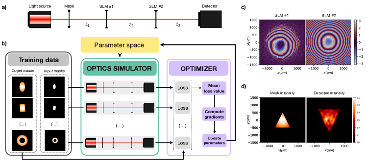
Figure 2: Rediscovery of the optical configuration employed to magnify images. (a) Virtual optical arrangement. Original lenses are replaced by two spatial light modulators (SLMs) with a resolution of $1024\times 1024$ and pixel size of $2.92\mu m$. The parameter space (of $\sim$ 2 million parameters) includes the distances, $z_{1}$, $z_{2}$ and $z_{3}$ (in millimeters) and the phase masks (in radians) of the two SLMs. (b) Data-driven discovery scheme. Input-output sample pairs are fed into the optics simulator in batches of 10. The loss function, computed for each virtual optical setup, evaluates the mean squared error between the intensity response of the system and the corresponding target example from the dataset. The average loss over the batch guides the optical parameter update, which is common to all the virtual optical setups. This cycle is repeated until convergence is reached. (c) Identified phase mask solutions for SLM$\#$1 and SLM$\#2$. They depict lens-like quadratic phases. Identified distances correspond to $z_{1}=5.81$ cm, $z_{2}=36.62$ cm and $z_{3}=55.92$ cm. This solution was identified in roughly 1 hour using a single GPU. (d) Input and detected intensity patterns for the identified optical design.

III Results

In this section, we showcase the virtual optical designs generated by XLuminA. As benchmarks, we aim to re-discover three foundational experiments, each one covering different areas in optics. By increasing the complexity of the description of light (from scalar to vectorial fields representation), we selected: (1) an optical configuration commonly used to adjust beam and image sizes, (2) beam shaping as employed in STED microscopy [10], and (3) the super-resolution technique using optical vortices detailed in Ref. [25]. Finally, we demonstrate the discovery of a new experimental blueprint within a large-scale exploration framework. For the first example, we use a data-driven learning methodology. For the last three, we set-up a discovery scheme where no training data is involved. The showcased solutions in both scenarios are the result from running multiple optimizations.

III.1 Data-driven rediscovery

The optical configuration to adjust beam and image sizes comprises two lenses, each one positioned a focal length apart from their respective input and output planes, $f_{1}$ and $f_{2}$, respectively, and $f_{1}+f_{2}$ from each other. This arrangement performs optical Fourier transformations of input light with magnifications determined by the ratio $f_{2}/f_{1}$. To revisit this design with a magnification of 2$\times$, we encoded the virtual setup depicted in Fig. 2a.

The data-driven learning approach is outlined in Fig. 2b. This workflow resembles the dynamics of training, in a supervised way, a physical neural network [51, 52]. The system dynamically adjusts the optical elements to effectively transform the input data into the desired configuration. The cost function is computed as

$$\mathcal{L}=\text{MSE}(I_{\text{Det}},I_{\text{GT}})\;,$$ (1)

where MSE is the mean squared error between the detected intensity pattern from the virtual setup, $I_{\text{Det}}$ and the corresponding ground truth from the dataset, $I_{\text{GT}}$. The parameter space comprises $1024\times 1024$ pixel phases and $3$ optical distances (a total of $\sim$ 2 million parameters). Further details of the optimization are provided in the Methods section.

The obtained results are displayed in Fig. 2c. The SLMs depict lens-like quadratic phases. Notably, the reference model traditionally uses two lenses set at specific distances, yet the identified distances don’t fulfill such relation. We validate the performance of the identified configuration by imaging the triangle-shaped amplitude mask shown in Fig. 2d, not included in the training data. The detected intensity distribution demonstrates that the optical setup can invert but not sufficiently magnify 2$\times$ the input shape, but roughly 1.5$\times$. Considering the parameter space contains 2 million phases and three distances, future implementations include a more refined tuning of the parameters, e.g., accordingly weighting different variables with distinct physical meaning. We believe adopting these strategies will significantly enhance the accuracy of the system.

III.2 Discovery through exploration

In this section we rediscover the complex optical setups of STED microscopy and the super-resolution technique using optical vortices. To do so, we conduct an exploration-based optimizing procedure which does not involve training examples.

The loss function, $\mathcal{L}$, is calculated as the inverse of the density of the total detected intensity over a certain threshold, $I_{\varepsilon}$. Thus, minimizing $\mathcal{L}$ aims to maximize the generation of small, high intensity beams. In particular,

$$\mathcal{L}=\frac{1}{\text{Density}}=\frac{\text{Area}}{I_{\varepsilon}}$$ (2)

where $I_{\varepsilon}$ is the sum of pixel intensity values greater than the threshold value $\varepsilon\cdot i_{\text{max}}$, where $0\leq\varepsilon\leq 1$ and $i_{max}$ corresponds to the maximum detected intensity. The Area corresponds to the total number of camera pixels fulfilling the same condition. Details on the derivation of the loss function are provided in the Methods section.

III.2.1 STED microscopy

STED microscopy [10, 53] is one of the first discovered techniques that circumvent the classical diffraction limit of light. The key idea of this technique is the use of two diffraction-limited laser beams, one probe to activate (excite) the light emitters of the sample and one, doughnut-shaped beam to deactivate its excitation in a controlled way (depletion). Thus, the ultimately detected light is that of the emitters laying in the central region of the doughnut-shaped beam. This effectively reduces the area of normal fluorescence, which leads to super-resolution imaging. To simulate one of the fundamental concepts of STED without having to rely on time-dependent processes, we perform a nonlinear modulation of the focused light based on the Beer-Lambert law [54], commonly used to describe the optical attenuation in light-matter interaction. The details of our model are provided in the Methods section.

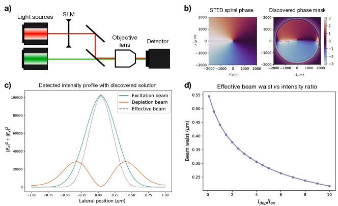
Figure 3: Rediscovery of beam-shaping technique as employed in STED microscopy. (a) Virtual optical setup. It consists of two light sources generating Gaussian beams corresponding to the depletion and excitation beams, linearly polarized in orthogonal directions, with wavelengths of $650$ nm and $532$ nm, respectively. Within the depletion beam’s optical path, we place an SLM with a resolution of $2048\times 2048$ and a computational pixel size of $1.95\mu m$. After propagating some set distance, a 0.9 NA objective lens focuses both light beams into the detector screen of $0.05\mu m$ pixel size. The parameter space for the optimization is defined by the SLM ($\sim$ 4.2 million parameters). (b) STED spiral phase (S. W. Hell and J. Wichmann, 1994) and discovered phase mask. This solution was found in roughly 7 minutes using a single GPU. (c) Radial intensity profile in vertical beam section: excitation (green), depletion (orange), and super-resolution effective STED beam (dotted blue). The excitation and depletion beams are diffraction-limited. The effective response breaks the diffraction limit. Lateral position indicates lateral distance from the optical axis. (d) Effective beam waist (in $\mu$m) as a function of depletion and excitation intensity ratio ($I_{dep}/I_{ex}$). We observe the expected inverse square root scaling as originally demonstrated in STED microscopy.

To revisit this principle, we virtually construct a simplified version of a STED-type setup topology as depicted in Fig. 3a. The loss function corresponds to equation (2) considering the radial component of the effective beam, resulting from the STED process. The parameter space corresponds to $2048\times 2048$ pixel phases, a total of $\sim$ 4.2 million parameters. In Fig. 3b, we present the reference spiral phase mask and the identified solution. To highlight the doughnut shape of the depletion beam, we compute the vertical cross-section of the focused intensity patterns for both excitation and depletion beams (green and orange lines in Fig. 3c, respectively) and the effective beam (dotted blue line in Fig. 3c). The behavior across the horizontal axis yields similar features. In addition, we systematically change the relative beam intensities as depicted in 3d. We observe the inverse square root scaling of the effective beam diameter relative to the intensity ratio as demonstrated for STED microscopy [10].

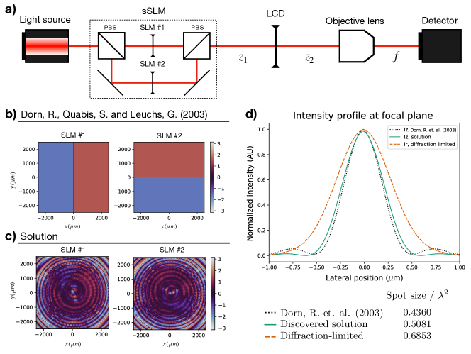
Figure 4: Optical design and rediscovery of the super-resolution technique employing optical vortices to generate a longitudinal sharp focus. (a) Virtual optical setup consisting of a light source emitting a $635$ nm wavelength Gaussian beam that is linearly polarized. The original optical elements are replaced by an super-SLM, which consists of two SLMs, each one independently imprinting a phase mask on the horizontal and vertical polarization components of the field. PBS denotes for polarization beam splitter. Each component of the sSLM has a resolution of $2048\times 2048$ pixels and a computational pixel size of $2.44$ $\mu m$. Additionally, we place an LCD with variable phase retardance $\eta$ and orientation angle $\theta$. The beam then passes through a 0.9 NA objective lens before reaching the detector screen of $0.05$ $\mu m$ pixel size; $z_{1}$ and $z_{2}$ denote for distances. The parameter space ($\sim$ 8.4 million parameters) is defined by the two SLMs, the LCD, and the distances. (b) Phase masks for simulating the reference experiment. The optical parameters for LCD are set to 0 and the distances $z_{1}$ and $z_{2}$ to $40$ mm and $3000$ mm, respectively. (c) Discovered phase patterns. Discovered optical parameters for LCD’s retardance, orientation, and propagation distances correspond to $-1.23$ rad, $2.32$ rad, $800$ mm and $710$ mm, respectively. This solution was identified in roughly 2 hours using a single GPU. (d) Longitudinal intensity profile, $|E_{z}|^{2}$, for Dorn, Quabis, and Leuchs (2003) and the identified solution (black dotted, and green lines, respectively) and radial intensity profile, $I_{r}$, of the diffraction-limited linearly polarized beam (orange dotted line). Lateral position indicates lateral distance from the optical axis. The spot size is computed as $\phi=(\pi/4)\text{FWHM}_{x}\text{FWHM}_{y}$. The discovered approach breaks the diffraction limit, demonstrating a similar spot size as the reference. Remarkably, it does not feature side lobes, which can limit practical imaging techniques.

III.2.2 Sharper focus with optical vortices

The final benchmark focuses on the generation of an ultra-sharp focus, a feature that breaks the diffraction limit in the longitudinal direction as demonstrated by Dorn, Quabis and Leuchs in Ref. [25]. This super-resolution is achieved when a radially polarized beam is tightly focused [55, 56]. To revisit this principle, we encoded the virtual setup depicted in Fig. 4a. The reference experiment is simulated using the phase masks in Fig. 4b. The loss function corresponds to equation (2) considering the measured intensity as the electromagnetic field’s longitudinal component. The parameter space contains $2\times(2048\times 2048)$ pixel phases, 2 optical parameters for extra optical modulation and 2 distances (a total of $\sim$ 8.4 million parameters). The detailed description of the optimization is provided in the Methods section. The discovered phase patterns are depicted in Fig. 4c. These produce an $LG_{2,1}$ Laguerre-Gaussian mode [57], which demonstrates an intensity pattern of concentric rings with a phase singularity in its center. Remarkably, XLuminA found an alternative way to imprint a phase singularity onto the beam and produce pronounced longitudinal components on the focal plane. The longitudinal intensity profiles for the reference and the discovered solution are depicted in Fig. 4d (represented by dotted black and green respectively). For comparison, we also feature the radial intensity profile of the diffraction-limited beam (dotted orange line in Fig. 4d). The identified solution showcases a radial intensity doughnut shape and surpasses the diffraction limit in the longitudinal component demonstrating a spot size slightly larger than the reference.

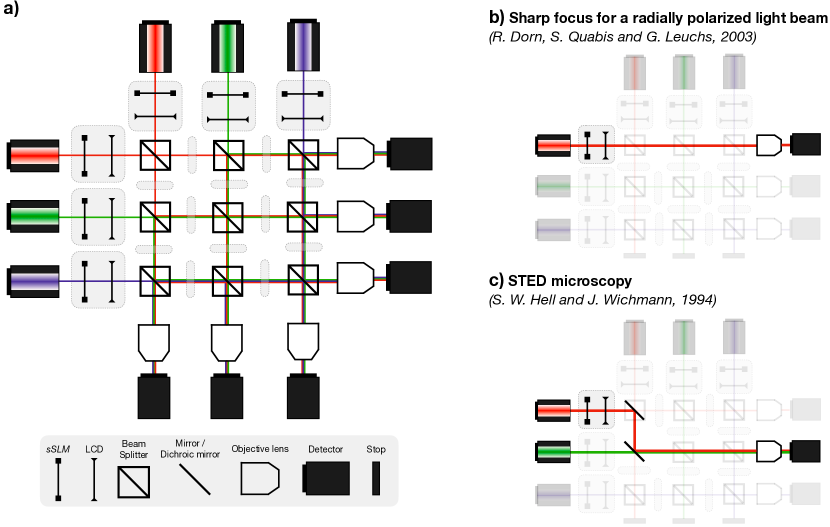
Figure 5: Large-scale optical discovery scheme and contained virtual setups. (a) General virtual optical setup for large-scale discovery schemes. Gray boxes represent fundamental building units, each containing a super-SLM and an LCD positioned a distance z apart. These units are inter-connected through free propagation distances and beam splitters. To ensure the illustration remains clear and not overly crowded, the building units positioned between beam splitters are depicted as thinner gray boxes. The setup’s complexity and size can be arbitrarily extended by incorporating additional connections, building units, light sources, detectors, etc. (b) Virtual optical setup for R. Dorn, S. Quabis and G. Leuchs, 2003. (c) Virtual optical setup for STED microscopy (S. W. Hell, and J. Wichmann, 1994).

III.3 Towards large-scale discovery

The results we have presented thus far predominantly involve optical setups characterized by a limited number of optical elements. This was crucial for our purpose to demonstrate how XLuminA can compute and efficiently rediscover known techniques in advanced microscopy. However, our ambition extends beyond the optimization. We aim to use XLuminA to discover new microscopy concepts. To achieve this, we initialize the setups with a large and complex optical topology, inspired by other fields that start with highly expressive initial circuits [58, 59]. From here, XLuminA should be able to extract much more complex solutions which humans might not have thought about yet [2].

In essence, discovering new experimental configurations entails an hybrid discrete-continuous search problem. The discrete aspect originates from configuring the optical network topology, whereas the continuous part is linked to the settings of optical elements, such as laser power and beam splitter reflectivity. Discrete-continuous optimization is extremely difficult computationally, therefore we invent a way to translate this problem into a purely continuous optimization problem which can be solved with efficient gradient-based methods. As illustrated in Fig. 5a, our goal is now to discover both the optical topology together with the continuous setting in a large, quasi-universal computational ansatz setup. Figure 5b and c illustrate how the topologies of the two main super-resolution examples (Dorn, Quabis, Leuchs [25] and STED [10]) are special cases inside our ansatz, and it allows for a large number of other optical topologies. The task of XLuminA is to automatically discover new superior topologies together with their parameter setting, using purely continuous optimization. For further analysis, we evaluate the efficiency of XLuminA by measuring the computational time it takes to construct the optical setup in Fig. 5a and comparing it with respect to Diffractio. The resulting times, measured across various resolutions, are depicted in Extended Data Fig. 3.

Diffractio exhibits a notable exponential increase in its running time, showing times of 6 minutes for high resolution pixel arrays of $1024\times 1024$. Remarkably, for the same resolution, XLuminA demonstrates better scaling in CPU, operating at 2.5 minutes. On the GPU, XLuminA’s performance is 60 times faster than Diffractio. The detailed analysis is provided in the Methods section.

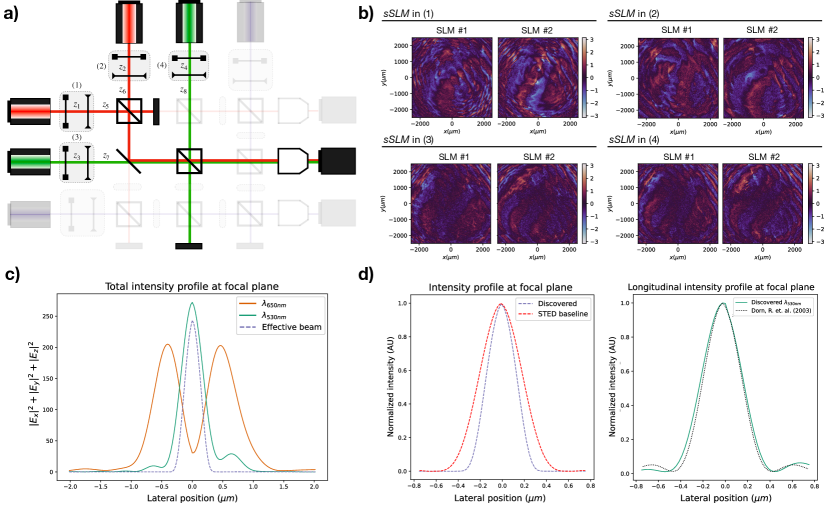
Figure 6: Discovery of a new experimental blueprint within a large-scale optical setup. (a) Scheme of the virtual optical setup utilized for testing the large-scale discovery framework. It features light sources that emit Gaussian beams with wavelengths of $650$ nm and $530$ nm, both linearly polarized at $45^{o}$. Gray boxes, numbered from (1) to (4), represent the building units, each comprising one sSLM and one LCD . Distances are denoted as $z_{i}$ where $i=1,...,8$. The beam splitters are set to $50/50$ transmittance/reflectance. The resolution is set to $1024\times 1024$ pixels with a pixel size of $4.8\mu m$. The 0.9 NA objective lens focuses the light onto the detector of $0.05\mu m$ pixel size. The parameter space ($\sim$ 8.4 million parameters) contains four sSLM, four LCDs with variable phase retardance $\eta$ and orientation angle $\theta$, and eight distances. (b) Discovered phase masks corresponding to the four sSLM within building units from (1) to (4). The identified optical parameters are: for the LCD in (1): $\eta=3.63$, $\theta=1.76$; in (2): $\eta=-1.44$, $\theta=-0.03$; in (3): $\eta=-1.01$, $\theta=-2.25$; and (4): $\eta=0.75$, $\theta=-2.67$. The propagation distances ($z_{1}$ to $z_{8}$, in cm) are 50.41, 68.56, 96.26, 38.99, 22.18, 140.98, 25.97, and 43.40, respectively. This solution was found after roughly 17 minutes using a single GPU. (c) Total intensity vertical cross-section of the detected light beams of $650$ nm (orange), $530$ nm (green), and effective beam emulating stimulated emission (dotted blue). (d) Vertical cross-section of the normalized total intensity of the effective beam from the discovered solution (dotted blue) and the simulated STED reference (red dotted), and the longitudinal intensity comparison between the discovered $530$ nm (green) and the simulated reference for Dorn, Quabis, and Leuchs (2003) using the same $530$ nm wavelength.

Finally, we demonstrate the capability of XLuminA for genuine discovery through the virtual setup depicted in Fig. 6a. The loss function corresponds to equation (2) considering the total intensity of the effective beam resulting from the emulated STED process. The parameter space comprises $8\times(1024\times 1024)$ pixel phases, 8 extra optical modulation parameters and 8 distances (a total of $\sim$ 8.4 million parameters). The details of the optimization are provided in the Methods section. The identified solution is presented in Fig. 6b. The detected intensity topologies reveal the setup generates a doughnut-shaped and a Gaussian-like beams. To highlight these shapes, we compute the vertical cross-section of the focused intensity patterns for both beams and the resulting effective beam (green, orange and dotted blue lines in Fig. 6c, respectively). The horizontal cross-section exhibits analogous features. We further compare the effective beam intensity with the simulated STED reference [10] and the the discovered Gaussian-like beam with the simulated sharp focus reference [25]. The obtained results are showcased in Fig. 6d. Remarkably, the discovered solution exploits the underlying physical concepts of two aforementioned optical systems. In one hand, it generates a doughnut-shaped “depletion” beam as demonstrated in STED microscopy. On the other hand, it generates a Gaussian-like “excitation” signal with a sharper focus, achieving smaller effective intensity spots resulting from the STED process. Remarkably, the discovered solution showcases an effective beam profile which is sharper than the simulated reference in Fig. 3d. This occurs due to the enhanced sharpening of the longitudinal component of the excitation beam, which demonstrates similar profile as the simulated reference in Fig. 4d. Regardless of its physical realizability, this solution demonstrates the ability of XLuminA to uncover interesting solutions within highly complex systems.

IV Discussion

In this work we present XLuminA, a highly efficient computational framework with seamlessly integrated auto-differentiation capabilities, just-in-time compilation, automatic vectorization and GPU compatibility, for the discovery of novel optical setups in super-resolution microscopy.

We demonstrate the high-performance and efficiency of XLuminA by the computational speed-up of two orders of magnitude for well-established light propagation algorithms, particularly powerful in scenarios that demand repeated calculations of optical setups, as seen in optimization tasks of generating extensive datasets for surrogate neural network models. Moreover, we prove XLuminA’s accuracy and reliability by rediscovering three foundational optical experiments. More significantly, within a large-scale discovery framework, XLuminA identified a novel experimental blueprint that breaks the diffraction limit by integrating the physical principles of two well-known super-resolution techniques.

We plan to significantly expand XLuminA’s optical simulator by adding more physical properties and features exploited in microscopy, for example, detailed coverage of frequency and time information, which might enable systems such as iSCAT [60], structured illumination microscopy [61], and localization microscopy [62]. Additionally, XLuminA provides already the basis for an expansion to complex quantum optics microscopy techniques [63] or other quantum imaging techniques [64], as a quantum of light (i.e., a photon) is nothing else than an excitation of the modes of the electromagnetic field. Looking further into the future, one can expect that matter-wave beams (governed by Schrödinger’s equation, which is closely related to the paraxial wave equation, a special case of the electromagnetic field) can be simulated in the same framework. This might allow for the AI-based design of hybrid microscopy techniques using light and complex electron-beams [65] or coherent beams of high-mass particles [66]. Ultimately, bringing so far unexplored concepts from diverse areas of physics to microscopy applications is at the heart of AI-driven discovery in this area, and we hope that this work constitutes a first step in this direction.

V Methods

V.1 Features and performance of XLuminA

In this section we provide the detailed description of XLuminA’s simulation features and performance. The simulator enables, among many other features, to define light sources (of any wavelength and power), phase masks (i.e., spatial light modulators, SLMs), polarizers, variable retarders (e.g., liquid crystal displays, LCDs), diffraction gratings, and high NA lenses to replicate strong focusing conditions. Light propagation and diffraction is simulated by two methods, each available for both scalar and vectorial regimes: the fast-Fourier-transform (FFT) based numerical integration of the Rayleigh-Sommerfeld (RS) diffraction integral [67, 68] and the Chirped z-transform (CZT) [69]. The CZT is an accelerated version of the RS algorithm, which allows for arbitrary selection and sampling of the region of interest. These algorithms are based on the FFT and require a reasonable sampling for the calculation to be accurate [70]. In our simulations we consider light sources emitting Gaussian beams of $1.2$ mm beam waist. To avoid possible boundary-generated artifacts during the simulation, we define these beams in larger computational spaces of $4$ mm or $5$ mm. Thus, the pixel resolutions often span $1024\times 1024$, or $2048\times 2048$.

Some functionalities of XLuminA’s optics simulator (e.g., optical propagation algorithms, planar lens or amplitude masks) are inspired in an open-source NumPy-based Python module for diffraction and interferometry simulation, Diffractio [42], although we have rewritten and modified these approaches to combine them with JAX just-in-time (jit) functionality. On top of that, we developed completely new functions (e.g., beam splitters, LCDs or propagation through high NA objective lens with CZT methods, to name a few) which significantly expand the software capabilities. The most important hardware addition on the optical simulator are the SLMs, each pixel of which possesses an independent (and variable) phase value. They serve as a universal approximation for phase masks, including lenses, and offer a computational advantage: given a specific pixel resolution, they allow for unrestricted phase design selection. Such flexibility is crucial during the parameter space exploration, as it allows the software to autonomously probe all potential solutions. In addition, we defined under the name of super-SLM (sSLM) a hardware-box-type which consists of two SLMs, each one independently imprinting a phase mask on the horizontal and vertical polarization components of the field.

To evaluate the performance of numerical and auto-differentiation methods we chose to use BFGS (from SciPy’s Python library) and ADAM (included in the JAX library) as optimizers. We set-up a Gaussian beam interacting with a phase mask as the optical system. The objective function is the mean squared error between the detected light and the ground truth, characterized by a Gaussian beam with a spiral phase imprinted on its wavefront. We initialize the system with an arbitrary phase mask configuration. We first evaluate the computational time for a single gradient evaluation for numerical and autodiff methods across different computational window sizes (from $10\times 10$ up to $150\times 150$ pixels) and devices (CPU and GPU). We keep the default settings for BFGS. For ADAM, the step size is set to 0.01. The optimization process is terminated if there is no improvement in the loss value (meaning it has not decreased below the best value recorded), over 50 consecutive iteration steps. For each resolution window, we collect the convergence time of both optimizers and divide it by the total number of gradient evaluations for BFGS and the total number of steps for ADAM. The acquired gradient evaluation times correspond to the mean value over 5 runs. Obtained results are depicted in Fig. 1c. It is clear how autodiff outperforms numerical methods by one up to two orders of magnitude in CPU for small computational window sizes (from $10\times 10$ to $70\times 70$ pixels). The difference is even more pronounced (4 orders of magnitude) for computational windows larger than $80\times 80$ pixels. The gradient evaluation for autodiff is even faster (one order of magnitude faster than for CPU) when running in the GPU. Although there exists some overhead for the small computational window size of $10\times 10$ pixels, the advantage over larger sizes is clear given that we run simulations with resolutions of $1024\times 1024$ and $2024\times 2048$ pixels.

We then conduct the evaluation of the convergence time for both methods. We keep the aforementioned settings for the optimizers. In this case, we evaluate for higher resolutions (from $10\times 10$ up to $500\times 500$ pixels). We initialize the systems 5 times and compute their mean value. The acquired results are depicted in Fig. 1d. On the CPU, numerical methods exhibit exponential scaling in convergence time, reaching about 6500 seconds (roughly 2 hours) for $250\times 250$ pixel window. In contrast, autodiff demonstrates superior efficiency, reducing it to roughly 2600 seconds (43 minutes). GPU optimization performance is even more pronounced, reaching convergence in approximately 120 seconds (2 minutes) for $250\times 250$ pixels, and 950 seconds (15 minutes) for a resolution of $500\times 500$.

V.2 Data-driven rediscovery

In this section we provide the details of the data-driven learning approach outlined in Fig. 2b. The training dataset is composed of $18,000$ [input, output] intensity sample pairs. Each sample consists of a Gaussian beam shaped by amplitude masks in various forms (circles, rectangles, squares and rings), with varying sizes and orientations. The corresponding output for each input is an inverted version, magnified by a factor of 2. The training process involves feeding the input mask into the virtual optical setup. The cost function for each optical setup is computed as the mean squared error between the detected intensity pattern from the virtual setup and the corresponding target mask from the dataset. We select training examples in batches of 10 and evaluate the current setup response and its loss value. The average loss over the batch guides the update of the optical parameters, repeating this cycle until convergence is reached. The parameter space (of $\sim$ 2 million parameters) includes the three distances and the phase masks of the two SLMs with a resolution of $1024\times 1024$ pixels. We set-up the ADAM optimizer with a step size of 0.1. The optimization is terminated if there is no improvement in the loss value (i.e., it has not decreased below the best value recorded), over 500 consecutive iteration steps. This condition is checked every 500 steps. We start the optimization with randomly initialized optical parameters with values between (0,1). The discovered solution is depicted in Fig. 2c. It was identified in about $50$ minutes on the GPU. The loss value evolution over the number of iteration steps is depicted in Extended Data Fig. 2a.

V.3 Stimulated emission depletion model

STED microscopy [10, 53] is based on excitation and spatially targeted depletion of fluorophores. In order to achieve this, a Gaussian-shaped excitation beam and a doughnut-shaped depletion beam (generated by imprinting a spiral phase into its wavefront) are concentrically overlapped. The depletion beam has zero intensity in the center, where the excitation beam has its maximum. Fluorophores that are not in the center of the beams are forced to emit at the wavelength of the depletion beam. Their emission is spectrally filtered out. Only fluorophores in the center of the beams are allowed to fluoresce normally, and only their emission is ultimately detected. This effectively reduces the area of normal fluorescence, which leads to super-resolution imaging.

We simulate one of the fundamental concepts of STED microscopy without having to rely on time-dependent processes related to absorption and fluorescence. To do so, we perform a nonlinear modulation of the intensity of the excitation and depletion beams based on the Beer-Lambert law [54]. We define the effective fluorescence that would ultimately be detected as:

$$I_{\text{eff}}=I_{\text{ex}}\left[1-\beta\left(1-e^{-(I_{\text{dep}}/I_{\text{ex})}}\right)\right]\;,$$ (3)

where $I_{\text{ex}}$ and $I_{\text{dep}}$ correspond to the excitation and depletion intensities, respectively, and $0\leq\beta\leq 1$ captures the quenching efficiency of the depletion beam. This expression bounds the effect of the depletion beam such that scenarios with negative effective intensity or unrealistically high values are avoided. In particular, assuming a perfect efficiency of the depletion beam in suppressing the excitation (i.e., $\beta=1$), we obtain an expression resembling the Beer-Lambert law:

$$I_{\text{eff}}=I_{\text{ex}}\cdot e^{-(I_{\text{dep}}/I_{\text{ex})}}\;.$$ (4)

Thus, the effective detected light falls off exponentially with the intensity ratio $I_{\text{dep}}/I_{\text{ex}}$. In the limit case where there is no excitation intensity, $I_{\text{ex}}=0$, the detected light is zero as well, $I_{\text{eff}}=0$. If there is no depletion intensity, $I_{\text{dep}}=0$, the detected light corresponds to the excitation beam $I_{\text{eff}}=I_{\text{ex}}$. The trivial case of null efficiency in the quenching, $\beta=0$, leads to the same result.

To evaluate the nonlinear effect we consider $\beta=1$ and $I_{\text{dep}}=\frac{1}{2}I_{\text{ex}}$. From equation (3) we obtain

$$I_{\text{eff}}=I_{\text{ex}}e^{-1/2}\approx 0.6I_{\text{ex}}\;.$$ (5)

Now, by slightly increasing the depletion energy, e.g., $I_{\text{dep}}=\frac{3}{2}I_{\text{ex}}$, it reads

$$I_{\text{eff}}=I_{\text{ex}}e^{-3/2}\approx 0.2I_{\text{ex}}\;.$$ (6)

Therefore, a small change in the depletion energy causes a large effect in the effective intensity. As a further example, if we set an intermediate efficiency of $\beta=0.5$ and $I_{\text{dep}}=\frac{1}{2}I_{\text{ex}}$ we obtain

$$I_{\text{eff}}=I_{\text{ex}}\left[\frac{1+e^{-1/2}}{2}\right]\approx 0.8I_{\text{ex}}\;.$$ (7)

which clearly demonstrates the effect of diminishing the efficiency of the suppression. Overall, we successfully imprinted the nonlinear behavior of the quenching for different range of effectiveness, achieving a realistic, bounded physical model for STED.

V.4 Discovery through exploration

In this section we detail the methodology for the optimizations within the discovery framework. We first detail the derivation of the loss function in equation (2). Then we provide the details for running the optimizations for STED microscopy and the super-resolution technique exploiting light vortices.

V.4.1 Loss function

The loss function, $\mathcal{L}$, is inversely proportional to the total detected intensity density that is above a specified intensity threshold, $I_{\varepsilon}$. Thus, minimizing $\mathcal{L}$ aims to maximize the generation of small, high intensity beams. In particular, it reads

$$\mathcal{L}=\frac{1}{\text{Density}}=\frac{\text{Area}}{I_{\varepsilon}}\;.$$ (8)

The total intensity $I_{\varepsilon}$ above the threshold is computed as

$$I_{\varepsilon}=\sum_{k,l}^{N}i_{\varepsilon}(k,l)\;,$$ (9)

where $N$ is the total number of pixels in the camera’s sensor and $i_{\varepsilon}(k,l)$ represents the intensity value at each pixel once the threshold condition is applied. This condition is defined as follows:

$$i_{\varepsilon}(k,l)=\begin{cases}i_{\text{det}}(k,l)&\text{if }i_{\text{det}}(k,l)>\varepsilon i_{\text{max}}\;,\\ 0&\text{otherwise}\;,\end{cases}$$ (10)

where $i_{\text{det}}(k,l)$ is the intensity value at the i-th row and j-th column in the detected 2D intensity pattern, $\varepsilon i_{\text{max}}$ (with $0\leq\varepsilon\leq 1$) is the threshold value, with $i_{\text{max}}$ being the maximum intensity value in the entire 2D detector array.

The Area is determined using a variation of the Heaviside function $\Theta$ applied to $i_{\varepsilon}$, quantifying the area where the intensity is above the threshold:

$$\text{Area}=\sum_{k,l}^{N}\Theta(i_{\varepsilon}(k,l))\;,$$ (11)

where $N$ is the total number of pixels in the camera’s sensor and $\Theta(i_{\varepsilon}(k,l))$ is defined as:

$$\Theta(i_{\varepsilon}(k,l))=\begin{cases}1&\text{if }i_{\varepsilon}(k,l)>0\;,\\ 0&\text{otherwise}\;.\end{cases}$$ (12)

Therefore, the loss function can be read as follows:

$$\mathcal{L}=\frac{1}{\text{Density}}=\frac{\text{Area}}{I_{\varepsilon}}=\frac{\sum_{k,l}^{N}\Theta(i_{\varepsilon}(k,l))}{\sum_{k,l}^{N}i_{\varepsilon}(k,l)}\;.$$ (13)

V.4.2 STED microscopy

In this section we provide details on the optimization for the beam shaping as employed in STED microscopy. In this instance, the parameter space corresponds to the $2048\times 2048$ pixels of the SLM ($\sim$ 4 million parameters), with a pixel size of $1.95\mu m$. The loss function corresponds to equation (2) considering the radial component of the effective beam, $|E_{x}|^{2}+|E_{y}|^{2}$ and $\varepsilon=0.7$. We simulate the stimulated emission depletion effect, using equation (3) with the efficiency set to $\beta=1$.

We set-up the ADAM optimizer with a step size of 0.01 and initialize the system in a random initial phase mask. The optimization is terminated if there is no improvement in the loss value over 500 consecutive iteration steps. This condition is checked every 100 steps. The identified solution is depicted in Fig. 3b. The system converged into a pattern alike to the spiral phase in roughly 7 minutes using a single GPU. The loss value evolution over the number of iteration steps is depicted in Extended Data Fig. 2b.

While the spiral phase mask features a consistent and gradual phase variation across the spiral, this progression is not as evident in the discovered solution. Furthermore, we would like to emphasize the remarkably low noise contribution on the identified phase pattern. Other solutions presented noisy phase patterns which failed to achieve the essential doughnut-shaped depletion beam. Real-world STED setups demand almost perfect phase patterns and alignment of components; even minor errors can compromise STED. Remarkably, without prior knowledge, our system detected this sensitivity, converging towards a smooth phase pattern. Moreover, despite both the excitation and depletion beams being diffraction-limited, the effective response is sub-diffraction. Such outcomes accentuate the success of XLuminA in identifying crucial components intrinsic to STED microscopy.

V.4.3 Sharper focus with optical vortices

In this section we provide details on the optimization for the super-resolution technique employing optical vortices. In this instance, the parameter space is defined by two SLMs with a resolution of $2048\times 2048$ pixels with a pixel size of $2.44\mu m$ each, one LCD with with variable phase retardance $\eta$ and orientation angle $\theta$, and three distances ($\sim$ 8.4 million parameters). The loss function corresponds to equation (2) considering the intensity of the longitudinal component $|E_{z}|^{2}$, and $\varepsilon=0.7$.

We set-up the ADAM optimizer with a step size of 0.03 and initialize the system with random optical parameters with values between (0,1). The stopping condition for the optimizer is the same as for STED microscopy: the optimization is terminated if there is no improvement in the loss value over 500 consecutive iteration steps. This condition is checked every 100 steps. The identified solution is depicted in Fig. 4c. The system converged after roughly 2 hours using a single GPU. The loss value evolution over the number of iteration steps is depicted in Extended Data Fig. 2c.

V.5 Large-scale discovery

In this section we first provide the details on the procedure for evaluating XLuminA’s performance in building large-scale optical setups. Then, we detail the optimization settings used for the large-scale discovery scheme.

The large-scale optical setup depicted in Fig. 5a consists of six polarized light sources that emit linearly polarized Gaussian beams with different wavelengths (625 nm, 530 nm and 470 nm). Through 82 vectorial propagation (vectorial Rayleigh-Sommerfeld, VRS), these beams interact with a total of 19 sSLM, 19 LCDs, 9 beam splitters, and 6 high NA objective lenses. We evaluate the efficiency of XLuminA by measuring the computational time it takes to construct this setup and comparing it with respect to Diffractio across different resolutions (from $10\times 10$ to $1024\times 1024$ pixels) and devices (CPU and GPU). The resulting times, measured across varying computational window sizes, are depicted in Extended Data Fig. 3.

Diffractio exhibits a notable exponential increase in its computational time past the size of $300\times 300$ pixels, showing running times of almost 6 minutes for a resolution of $1024\times 1024$ pixels. For smaller sizes, the efficiency of NumPy’s dispatch overhead times becomes relevant, making it faster in such regimes. In fact, when considering resolutions up to $200\times 200$ pixels, XLuminA experiences significant overhead times (on both CPU and GPU). These are attributed to JAX’s dispatch overhead. Although this time is independent of the size of the arrays, it becomes more pronounced when multiple operations are performed on smaller arrays. However, as array size increases, the dispatch costs diminish, highlighting the benefits of JAX’s accelerated linear algebra and just-in-time compilation. When running in CPU, XLuminA outperforms Diffractio, exhibiting superior scalability in both initial and subsequent runs. For example, for $1024\times 1024$ pixels, XLuminA operates in nearly half the time (2.5 minutes) required by Diffractio. This advantage becomes even more pronounced when XLuminA operates on a GPU. The initial run times remain fairly consistent across various computational window sizes, ranging from 14 to 16 seconds. Subsequent runs exhibit similar consistency, with times around 3 to 3.7 seconds up to $500\times 500$ pixels and 6 seconds for $1024\times 1024$ pixels.

Finally, we conduct an optimization for large-scale discovery on the complex setup in Fig. 6a. In this instance, the parameter space ($\sim$ 8.4 million parameters) corresponds to four super-SLMs (i.e., 8 SLMs) with a resolution of $1024\times 1024$ pixels with a pixel size of $4.8\mu m$, four LCDs and eight distances. The loss function corresponds to equation (2), in this instance considering the the total intensity of the effective beam, $|E_{x}|^{2}+|E_{y}|^{2}+|E_{z}|^{2}$, and $\varepsilon=0.5$. We simulate the stimulated emission depletion effect using equation (3) with the efficiency set to $\beta=1$.

We set-up the ADAM optimizer with a step size of 0.01 and initialize the system with random optical parameters with values between (0,1). The stopping condition for the optimizer is the same used for the two SR-techniques of STED microscopy and the sharp focus: the optimization is terminated if there is no improvement in the loss value over 500 consecutive iteration steps. This condition is checked every 100 steps. The identified phase masks are depicted in Fig. 6b. The system converged into a STED-like behavior in roughly 17 minutes using a single GPU. The loss value evolution over the number of iteration steps is depicted in Extended Data Fig. 2d.

VI Code availability

The produced code and documentation can be found via GitHub at https://github.com/artificial-scientist-lab/XLuminA.

Extended data

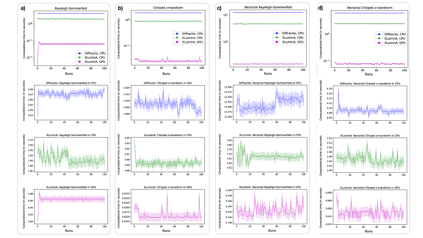
Extended Data Fig. 1: Execution time over 100 runs, within a resolution of $2048\times 2048$ pixels for the propagation methods of, in columns, (a) Rayleigh-Sommerfeld, (b) Chirped z-transform, (c) Vectorial Rayleigh-Sommerfeld and (d) Vectorial Chirped z-transform. Times for Diffractio are depicted in blue dots. First row corresponds to the log-scale representation. Times for XLuminA in CPU and GPU correspond to green triangles and magenta squares, respectively. Shades denote for the standard deviations values. Among the minor oscillations of the running times, the Rayleigh-Sommerfeld algorithm behavior stands out. When running in Diffractio, it shows an increase of the execution time of 0.005 seconds from the first run to subsequent runs. Similar behavior can be observed for the Rayleigh-Sommerfeld (RS) algorithm in XLuminA when executing in the GPU. This time, however, the increase occurs during the first 5 runs, from an first execution time of 0.0047 seconds to stabilize in 0.06 seconds for subsequent runs. This behavior is not present when executing XLuminA’s RS in the CPU. The origin of this factor of 10 is still unknown. We believe a further optimization on the RS propagation algorithm will improve the execution time.

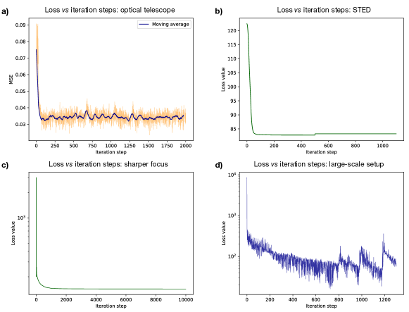
Extended Data Fig. 2: Loss value over iteration steps for (a) the optical system used to adjust beam and image sizes (i.e., an optical telescope), (b) the virtual STED setup, (c) the sharper focus employing optical vortices, and (d) the large-scale discovery setup.

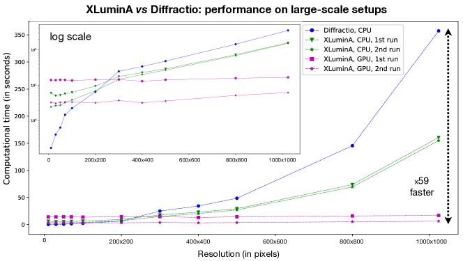
Extended Data Fig. 3: Computational time (in seconds) for generating the large-scale setup for Diffractio (blue dots) and XLuminA across different resolutions in CPU (green triangles) and GPU (magenta squares). For XLuminA, first run curves are decorated with triangles and second runs (pre-compiled jitted functions) with stars. Diffractio exhibits a notable exponential increase in its computational time, showing running times of almost 6 minutes for a resolution of $1024\times 1024$. When running in CPU, XLuminA outperforms Diffractio, exhibiting superior scalability in both initial and subsequent runs. For example, for $1024\times 1024$ pixels, XLuminA operates in nearly half the time (2.5 minutes) required by Diffractio. This advantage becomes even more pronounced when XLuminA operates on the GPU, demonstrating a speedup factor of $\times$59 for a resolution of $1024\times 1024$ pixels.

References

- Wang et al. [2023] H. Wang, T. Fu, Y. Du, W. Gao, K. Huang, Z. Liu, P. Chandak, S. Liu, P. Van Katwyk, A. Deac, et al., Scientific discovery in the age of artificial intelligence, Nature 620, 47 (2023).
- Krenn et al. [2022] M. Krenn, R. Pollice, S. Y. Guo, M. Aldeghi, A. Cervera-Lierta, P. Friederich, G. dos Passos Gomes, F. Häse, A. Jinich, A. Nigam, et al., On scientific understanding with artificial intelligence, Nature Reviews Physics 4, 761 (2022).
- Wollman et al. [2015] A. J. M. Wollman, R. Nudd, E. G. Hedlund, and M. C. Leake, From animaculum to single molecules: 300 years of the light microscope, Open Biology 5 (2015).
- Reigoto et al. [2021] A. M. Reigoto, S. A. Andrade, M. C. R. R. Seixas, M. L. Costa, and C. Mermelstein, A comparative study on the use of microscopy in pharmacology and cell biology research, PLOS ONE 16, 1 (2021).
- Weisenburger and Sandoghdar [2015] S. Weisenburger and V. Sandoghdar, Light microscopy: an ongoing contemporary revolution, Contemporary Physics 56, 123 (2015).
- Bullen [2008] A. Bullen, Microscopic imaging techniques for drug discovery, Nature Reviews Drug Discovery 7, 54 (2008).
- Antony et al. [2013] P. Antony, C. Trefois, A. Stojanovic, A. Baumuratov, and K. Kozak, Light microscopy applications in systems biology: opportunities and challenges, Cell Communication and Signaling 11 (2013).
- Grimm and Lavis [2022] J. B. Grimm and L. D. Lavis, Caveat fluorophore: an insiders’ guide to small-molecule fluorescent labels, Nature Methods 19 (2022).
- M. and Palmer [2014] D. K. M. and A. E. Palmer, Advances in fluorescence labeling strategies for dynamic cellular imaging, Nature Chemical Biology 10 (2014).
- Hell and Wichmann [1994] S. W. Hell and J. Wichmann, Breaking the diffraction resolution limit by stimulated emission: stimulated-emission-depletion fluorescence microscopy, Optics Letters 19, 780 (1994).
- Betzig et al. [2006] E. Betzig, G. H. Patterson, R. Sougrat, O. W. Lindwasser, S. Olenych, J. S. Bonifacino, M. W. Davidson, J. Lippincott-Schwartz, and H. F. Hess, Imaging intracellular fluorescent proteins at nanometer resolution, Science 313, 1642 (2006).
- Hess et al. [2006] S. T. Hess, T. P. Girirajan, and M. D. Mason, Ultra-high resolution imaging by fluorescence photoactivation localization microscopy, Biophysical Journal 91, 4258 (2006).
- Rust et al. [2006] M. Rust, M. Bates, and X. Zhuang, Sub-diffraction-limit imaging by stochastic optical reconstruction microscopy (storm), Nature Methods 3, 793–796 (2006).
- van de Linde et al. [2011] S. van de Linde, A. Löschberger, T. Klein, M. Heidbreder, S. Wolter, M. Heilemann, and M. Sauer, Direct stochastic optical reconstruction microscopy with standard fluorescent probes, Nature Protocols 6, 991–1009 (2011).
- Gustafsson [2005a] M. G. L. Gustafsson, Nonlinear structured-illumination microscopy: Wide-field fluorescence imaging with theoretically unlimited resolution, Proceedings of the National Academy of Sciences 102, 13081 (2005a).
- Balzarotti et al. [2017] F. Balzarotti, Y. Eilers, K. C. Gwosch, A. H. Gynnå, V. Westphal, F. D. Stefani, J. Elf, and S. W. Hell, Nanometer resolution imaging and tracking of fluorescent molecules with minimal photon fluxes, Science 355, 606 (2017).
- Möckl et al. [2019] L. Möckl, K. Pedram, A. R. Roy, V. Krishnan, A.-K. Gustavsson, O. Dorigo, C. R. Bertozzi, and W. Moerner, Quantitative super-resolution microscopy of the mammalian glycocalyx, Developmental Cell 50, 57 (2019).
- Xu et al. [2013] K. Xu, G. Zhong, and X. Zhuang, Actin, spectrin, and associated proteins form a periodic cytoskeletal structure in axons, Science 339, 452 (2013).
- Yildiz et al. [2003] A. Yildiz, J. N. Forkey, S. A. McKinney, T. Ha, Y. E. Goldman, and P. R. Selvin, Myosin v walks hand-over-hand: Single fluorophore imaging with 1.5-nm localization, Science 300, 2061 (2003).
- Zhang et al. [2015] Y. Zhang, J. M. Lucas, P. Song, B. Beberwyck, Q. Fu, W. Xu, and A. P. Alivisatos, Superresolution fluorescence mapping of single-nanoparticle catalysts reveals spatiotemporal variations in surface reactivity, Proceedings of the National Academy of Sciences 112, 8959 (2015).
- Müller et al. [2019] P. Müller, R. Müller, L. Hammer, C. Barner-Kowollik, M. Wegener, and E. Blasco, Sted-inspired laser lithography based on photoswitchable spirothiopyran moieties, Chemistry of Materials 31, 1966 (2019).
- Bradbury et al. [2018] J. Bradbury, R. Frostig, P. Hawkins, M. J. Johnson, C. Leary, D. Maclaurin, G. Necula, A. Paszke, J. VanderPlas, S. Wanderman-Milne, and Q. Zhang, JAX: composable transformations of Python+NumPy programs (2018).
- Baydin et al. [2018] A. G. Baydin, B. A. Pearlmutter, A. A. Radul, and J. M. Siskind, Automatic differentiation in machine learning: a survey, Journal of Machine Learning Research 18, 1 (2018).
- Möckl et al. [2014] L. Möckl, D. C. Lamb, and C. Bräuchle, Super-resolved fluorescence microscopy: Nobel prize in chemistry 2014 for eric betzig, stefan hell, and william e. moerner, Angewandte Chemie International Edition 53, 13972 (2014).
- Dorn et al. [2003] R. Dorn, S. Quabis, and G. Leuchs, Sharper focus for a radially polarized light beam, Physical Review Letters 91, 233901 (2003).
- Herath et al. [2023] K. Herath, U. Haputhanthri, R. Hettiarachchi, H. Kariyawasam, R. N. Ahmad, A. Ahmad, B. S. Ahluwalia, C. U. S. Edussooriya, and D. N. Wadduwage, Differentiable microscopy designs an all optical phase retrieval microscope (2023), arXiv:2203.14944 [physics.optics] .
- Yanny et al. [2020] K. Yanny, N. Antipa, W. Liberti, S. Dehaeck, K. Monakhova, F. L. Liu, K. Shen, R. Ng, and L. Waller, Miniscope3d: optimized single-shot miniature 3d fluorescence microscopy, Light: Science & Applications 9 (2020).
- Nehme et al. [2020] E. Nehme, D. Freedman, R. Gordon, B. Ferdman, L. E. Weiss, O. Alalouf, T. Naor, R. Orange, T. Michaeli, and Y. Shechtman, Deepstorm3d: dense 3d localization microscopy and psf design by deep learning, Nature Methods 17, 734–740 (2020).
- Krenn et al. [2016] M. Krenn, M. Malik, R. Fickler, R. Lapkiewicz, and A. Zeilinger, Automated search for new quantum experiments, Phys. Rev. Lett. 116, 090405 (2016).
- Knott [2016] P. Knott, A search algorithm for quantum state engineering and metrology, New Journal of Physics 18, 073033 (2016).
- Ruiz-Gonzalez et al. [2022] C. Ruiz-Gonzalez, S. Arlt, J. Petermann, S. Sayyad, T. Jaouni, E. Karimi, N. Tischler, X. Gu, and M. Krenn, Digital discovery of 100 diverse quantum experiments with pytheus (2022), arXiv:2210.09980 [quant-ph] .
- Valcarce et al. [2023] X. Valcarce, P. Sekatski, E. Gouzien, A. Melnikov, and N. Sangouard, Automated design of quantum-optical experiments for device-independent quantum key distribution, Phys. Rev. A 107, 062607 (2023).
- Krenn et al. [2020] M. Krenn, M. Erhard, and A. Zeilinger, Computer-inspired quantum experiments, Nature Review Physics 2, 649 (2020).
- Killoran et al. [2019] N. Killoran, J. Izaac, N. Quesada, V. Bergholm, M. Amy, and C. Weedbrook, Strawberry Fields: A Software Platform for Photonic Quantum Computing, Quantum 3, 129 (2019).
- Molesky et al. [2018] S. Molesky, Z. Lin, A. Y. Piggott, W. Jin, J. Vucković, and A. W. Rodriguez, Inverse design in nanophotonics, Nature Photonics 12, 659 (2018).
- So et al. [2020] S. So, T. Badloe, J. Noh, J. Bravo-Abad, and J. Rho, Deep learning enabled inverse design in nanophotonics, Nanophotonics 9, 1041 (2020).
- Sapra et al. [2020] N. V. Sapra, K. Y. Yang, D. Vercruysse, K. J. Leedle, D. S. Black, R. J. England, L. Su, R. Trivedi, Y. Miao, O. Solgaard, et al., On-chip integrated laser-driven particle accelerator, Science 367, 79 (2020).
- Su et al. [2018] L. Su, A. Y. Piggott, N. V. Sapra, J. Petykiewicz, and J. Vuckovic, Inverse design and demonstration of a compact on-chip narrowband three-channel wavelength demultiplexer, ACS Photonics 5, 301 (2018).
- Hughes et al. [2018] T. W. Hughes, M. Minkov, I. A. D. Williamson, and S. Fan, Adjoint method and inverse design for nonlinear nanophotonic devices, ACS Photonics 5, 4781 (2018).
- Minkov et al. [2020] M. Minkov, I. A. D. Williamson, L. C. Andreani, D. Gerace, B. Lou, A. Y. Song, T. W. Hughes, and S. Fan, Inverse design of photonic crystals through automatic differentiation, ACS Photonics 7, 1729 (2020).
- Lesina et al. [2015] A. C. Lesina, A. Vaccari, P. Berini, and L. Ramunno, On the convergence and accuracy of the fdtd method for nanoplasmonics, Optics Express 23, 10481 (2015).
- Brea [2019] L. M. S. Brea, Diffractio, python module for diffraction and interference optics ((2019)).
- Freise et al. [2013] A. Freise, D. Brown, and C. Bond, Finesse, frequency domain interferometer simulation software (2013), arXiv:1306.2973 [physics.comp-ph] .
- Perrin et al. [2012] M. D. Perrin, R. Soummer, E. M. Elliott, M. D. Lallo, and A. Sivaramakrishnan, Simulating point spread functions for the james webb space telescope with webbpsf, Space Telescopes and Instrumentation 2012: Optical, Infrared, and Millimeter Wave 8442 (2012).
- Fontaine et al. [2019] N. K. Fontaine, R. Ryf, H. Chen, D. T. Neilson, K. Kim, and J. Carpenter, Laguerre-gaussian mode sorter, Nature Communications 10 (2019).
- Labroille et al. [2014] G. Labroille, B. Denolle, P. Jian, P. Genevaux, N. Treps, and J.-F. Morizur, Efficient and mode selective spatial mode multiplexer based on multi-plane light conversion, Opt. Express 22, 15599 (2014).
- Flam-Shepherd et al. [2022] D. Flam-Shepherd, T. C. Wu, X. Gu, A. Cervera-Lierta, M. Krenn, and A. Aspuru-Guzik, Learning interpretable representations of entanglement in quantum optics experiments using deep generative models, Nature Machine Intelligence 4, 544 (2022).
- [48] J. Nocedal and S. J. Wright, Numerical optimization (Springer).
- Kingma and Ba [2017] D. P. Kingma and J. Ba, Adam: A method for stochastic optimization (2017), arXiv:1412.6980 [cs.LG] .
- Virtanen et al. [2020] P. Virtanen, R. Gommers, T. E. Oliphant, M. Haberland, T. Reddy, D. Cournapeau, E. Burovski, P. Peterson, W. Weckesser, J. Bright, S. J. van der Walt, M. Brett, J. Wilson, K. J. Millman, N. Mayorov, A. R. J. Nelson, E. Jones, R. Kern, E. Larson, C. J. Carey, İ. Polat, Y. Feng, E. W. Moore, J. VanderPlas, D. Laxalde, J. Perktold, R. Cimrman, I. Henriksen, E. A. Quintero, C. R. Harris, A. M. Archibald, A. H. Ribeiro, F. Pedregosa, P. van Mulbregt, and SciPy 1.0 Contributors, SciPy 1.0: Fundamental Algorithms for Scientific Computing in Python, Nature Methods 17, 261 (2020).
- McMahon [2023] P. L. McMahon, The physics of optical computing, Nature Reviews Physics 10.1038/s42254-023-00645-5 (2023).
- Wright et al. [2022] L. G. Wright, T. Onodera, M. M. Stein, T. Wang, D. T. Schachter, Z. Hu, and P. L. McMahon, Deep physical neural networks trained with backpropagation, Nature 601, 549–555 (2022).
- Hofmann et al. [2005] M. Hofmann, C. Eggeling, S. Jakobs, and S. W. Hell, Breaking the diffraction barrier in fluorescence microscopy at low light intensities by using reversibly photoswitchable proteins, Proceedings of the National Academy of Sciences 102, 17565 (2005).
- Mayerhöfer et al. [2020] T. G. Mayerhöfer, S. Pahlow, and J. Popp, The bouguer‐beer‐lambert law: Shining light on the obscure, Chemphyschem 21, 2029 (2020).
- Quabis et al. [2000] S. Quabis, R. Dorn, M. Eberler, O. Glöckl, and G. Leuchs, Focusing light to a tighter spot, Optics Communications 179, 1 (2000).
- Quinteiro et al. [2017] G. F. Quinteiro, F. Schmidt-Kaler, and C. T. Schmiegelow, Twisted-light–ion interaction: The role of longitudinal fields, Phys. Rev. Lett. 119, 253203 (2017).
- Rubinsztein-Dunlop et al. [2016] H. Rubinsztein-Dunlop, A. Forbes, M. V. Berry, M. R. Dennis, D. L. Andrews, M. Mansuripur, C. Denz, C. Alpmann, P. Banzer, T. Bauer, E. Karimi, L. Marrucci, M. Padgett, M. Ritsch-Marte, N. M. Litchinitser, N. P. Bigelow, C. Rosales-Guzmán, A. Belmonte, J. P. Torres, T. W. Neely, M. Baker, R. Gordon, A. B. Stilgoe, J. Romero, A. G. White, R. Fickler, A. E. Willner, G. Xie, B. McMorran, and A. M. Weiner, Roadmap on structured light, Journal of Optics 19, 013001 (2016).
- Sim et al. [2019] S. Sim, P. D. Johnson, and A. Aspuru-Guzik, Expressibility and entangling capability of parameterized quantum circuits for hybrid quantum-classical algorithms, Advanced Quantum Technologies 2, 1900070 (2019).
- Krenn et al. [2021] M. Krenn, J. S. Kottmann, N. Tischler, and A. Aspuru-Guzik, Conceptual understanding through efficient automated design of quantum optical experiments, Phys. Rev. X 11, 031044 (2021).
- Taylor and Sandoghdar [2019] R. W. Taylor and V. Sandoghdar, Interferometric scattering microscopy: Seeing single nanoparticles and molecules via rayleigh scattering, Nano Letters 19, 4827 (2019).
- Gustafsson [2005b] M. G. L. Gustafsson, Nonlinear structured-illumination microscopy: Wide-field fluorescence imaging with theoretically unlimited resolution, Proceedings of the National Academy of Sciences 102, 13081 (2005b).
- Lelek et al. [2021] M. Lelek, M. T. Gyparaki, G. Beliu, F. Schueder, J. Griffié, S. Manley, R. Jungmann, M. Sauer, M. Lakadamyali, and C. Zimmer, Single-molecule localization microscopy, Nature Reviews Methods Primers 1 (2021).
- Taylor et al. [2013] M. A. Taylor, J. Janousek, V. Daria, J. Knittel, B. Hage, H.-A. Bachor, and W. P. Bowen, Biological measurement beyond the quantum limit, Nature Photonics 7, 229 (2013).
- Moreau et al. [2019] P.-A. Moreau, E. Toninelli, T. Gregory, and M. J. Padgett, Imaging with quantum states of light, Nature Reviews Physics 1, 367 (2019).
- Chirita Mihaila et al. [2022] M. C. Chirita Mihaila, P. Weber, M. Schneller, L. Grandits, S. Nimmrichter, and T. Juffmann, Transverse electron-beam shaping with light, Phys. Rev. X 12, 031043 (2022).
- Kiałka et al. [2022] F. Kiałka, Y. Y. Fein, S. Pedalino, S. Gerlich, and M. Arndt, A roadmap for universal high-mass matter-wave interferometry, AVS Quantum Science 4 (2022).
- Shen and Wang [2006] F. Shen and A. Wang, Fast-fourier-transform based numerical integration method for the rayleigh-sommerfeld diffraction formula, Applied Optics 45, 1102 (2006).
- Ye et al. [2013] H. Ye, C.-W. Qiu, K. Huang, J. Teng, B. Luk’Yanchuk, and S. Yeo, Creation of a longitudinally polarized subwavelength hotspot with an ultra-thin planar lens: Vectorial rayleigh-sommerfeld method, Laser Physics Letters 10 (2013).
- Hu et al. [2020] Y. Hu, Z. Wang, X. Wang, et al., Efficient full-path optical calculation of scalar and vector diffraction using the bluestein method, Light: Science & Applications 9, 119 (2020).
- Li et al. [2002] J. Li, Z. Fan, and Y. Fu, FFT calculation for Fresnel diffraction and energy conservation criterion of sampling quality, in Lasers in Material Processing and Manufacturing, Vol. 4915, edited by S. Deng, T. Okada, K. Behler, and X. Wang, International Society for Optics and Photonics (SPIE, 2002) pp. 180 – 186.