STELLA: Continual Audio-Video Pre-training with
Spatio-Temporal Localized Alignment

Abstract

Continuously learning a variety of audio-video semantics over time is crucial for audio-related reasoning tasks in our ever-evolving world. However, this is a nontrivial problem and poses two critical challenges: sparse spatio-temporal correlation between audio-video pairs and multimodal correlation overwriting that forgets audio-video relations. To tackle this problem, we propose a new continual audio-video pre-training method with two novel ideas: (1) Localized Patch Importance Scoring: we introduce a multimodal encoder to determine the importance score for each patch, emphasizing semantically intertwined audio-video patches. (2) Replay-guided Correlation Assessment: to reduce the corruption of previously learned audiovisual knowledge due to drift, we propose to assess the correlation of the current patches on the past steps to identify the patches exhibiting high correlations with the past steps. Based on the results from the two ideas, we perform probabilistic patch selection for effective continual audio-video pre-training. Experimental validation on multiple benchmarks shows that our method achieves a 3.69%p of relative performance gain in zero-shot retrieval tasks compared to strong continual learning baselines, while reducing memory consumption by $\sim$45%.

1 Introduction

Multimodal learning is an important problem for various real-world applications, as many real-world data types are multimodal, such as text-image (Liao et al., 2022; Lee et al., 2023), text-video (Villegas et al., 2022; Hu et al., 2022b), and audio-video (Korbar et al., 2018; Xiao et al., 2020) pairs. While most vision-language learning (Li et al., 2020; Yan et al., 2023; Liu et al., 2023) assumes the availability of curated multimodal data with human-annotated descriptions, audiovisual domain (Zhou et al., 2019; Gong et al., 2023) holds a unique and practical advantage, as most videos inherently come with accompanying audios without human annotations. Thanks to this property, audiovisual multimodal learning models can leverage web-scale raw videos (e.g., YouTube, TikTok, etc.) for training with minimal human efforts in data preprocessing, and thus have achieved impressive success in audio-video compositional reasoning (Tang et al., 2022; Huang et al., 2022a; Lin et al., 2023).

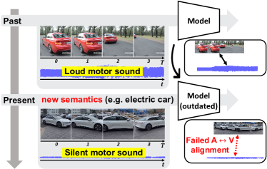
Figure 1: Outdated pre-trained audio-video models struggle with understanding emerging new audio-video semantics.

However, most existing approaches (Tang et al., 2022; Huang et al., 2022a; Gong et al., 2023) struggle when deployed to real-world scenarios, where the distribution of training data continuously changes over time with new audio-video semantics. For example, the audiovidual model pre-trained before electric vehicles became popular, would not be able to associate cars with their unique acoustic cues (e.g., motor sound) (See Fig. 1). One straightforward solution to this problem is to periodically train the model from scratch using audio-video data collected from the past to the present, but this approach comes with prohibitive computation and memory costs.

While continual learning is a viable solution for tackling such scenarios, dealing with dynamically evolving audio-video semantics is a nontrivial problem due to two critical challenges. First, the spatio-temporal correlation between the audio-video data is highly sparse. As represented in Fig. 2 (b), only a few objects/regions in a video (i.e., sound sources) are strongly correlated with audio. Secondly, audio-video pre-training models encounter the issue of forgetting not only the representations of each modality but also the correlation between them. As orange circles in Fig. 2 (c) illustrate, the model which initially learned the accurate audio-video correlation in a car’s engine video, forgets this correlation after learning on a series of audio-video tasks. It instead highlights inaccurate regions in the audio-video data, as if there were highly fine-grained multimodal alignment.

To overcome these challenges in learning multiple audio-video tasks sequentially, we propose Spatio-TEmporal LocaLized Alignment (STELLA), a novel approach that exploits past and current information via audio-video attention maps. Specifically, our goal is to continually pre-train the model by selecting audio and video patches that have a high correlation for its modality pair and also preserve previously learned audio-video correlation. Thereby we propose a probabilistic patch selection framework that enables the model to learn better audio-video correlations and preserve past audio-video semantics, based on two key components: first, we use the averaged cross-attention maps obtained by a lightweight multimodal encoder to compute an importance score, estimating how each audio (or video) patch is important for its modality pair. Further, to preserve the past correlation during continual audio-video pre-training, we leverage new cross-attention maps activated by the key and query embeddings between the current and past steps, respectively. This yields a correlation score that identifies the patches that exhibit a higher correlation with the current step than the past steps. We extensively validate our method on continual audio-video pre-training scenarios, using diverse benchmark datasets evaluated on various audiovisual downstream tasks. Our method outperforms strong baseline on various tasks with enhanced efficiency by reducing the GPU memory by $\sim$45% during continual pre-training. We further provide extensive in-depth analysis with visualizations.

Our paper makes the following key contributions:

• We are the first to address continual audio-video pre-training, which poses new challenges: sparse spatio-temporal correlation between audio-video pairs and multimodal correlation overwriting that forgets their relations.

• We propose a novel method that leverages cross-attention maps to capture sparse audio-video relationships and mitigate forgetting of previously learned relationships.

• We demonstrate the efficacy of our method on several audiovisual downstream tasks including retrieval, sound source localization and event localization. In particular, ours achieves 3.69%p of performance gain in the retrieval task and reduces the GPU memory consumption by $\sim$45% during training, compared to the strongest baseline.

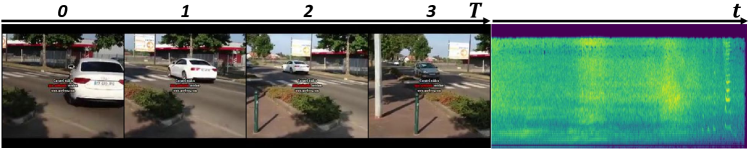
(a) Raw data

(b) Sparse audiovisual correlation

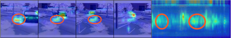
(c) Multimodal correlation forgetting (DER++)

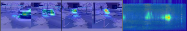
(d) Multimodal correlation forgetting (Ours)

Figure 2: Challenges in continual audio-video learning. (a): A raw data pair describing a car and its engine sound. (b): Sparse correlations in cross-attention maps. (c): After training on a series of tasks after (b), DER++ focuses on entirely different areas (orange circle), presenting correlation forgetting. (d): Our STELLA maintains consistent attention. More examples are in Fig. 16.

2 Related Work

Audiovisual understanding

Self-supervised learning on audiovisual data aims to learn transferable representations that can be applied to a variety of audio-image/video downstream tasks, including action recognition/event classification (Nagrani et al., 2021; Lee et al., 2021), sounding object localization (Hu et al., 2022a; Liu et al., 2022), and multimodal retrieval (Huang et al., 2022a; Gong et al., 2023). Inspired by the success of Masked AutoEncoders (MAE) in visual pre-training (He et al., 2022), recent audiovisual representation learning adopts masked modeling for comprehending audiovisual semantics (Tang et al., 2022; Gong et al., 2023). TVLT (Tang et al., 2022) adopts the MAE structure and audiovisual matching to predict whether audio and visual data originated from the same video. CAV (Gong et al., 2023) combines the MAE with audiovisual contrastive learning, which pulls matching audiovisual pairs closer and pushes non-matching pairs apart. Their methods assume a fixed input data distribution that does not shift throughout training. However, in the real world, a machine/agent will continuously encounter new (i.e., changing distribution) audio-video tasks/semantics. If not well managed, the methods will suffer severe performance degradation if they encounter the aforementioned shift in continual learning, a challenging and realistic scenario for multimodal learning.

Multimodal continual learning

Continual learning (Kirkpatrick et al., 2016; Rebuffi et al., 2017; Ahn et al., 2019) refers to a learning paradigm in which a model sequentially learns an unlimited number of tasks/domains. It aims to continuously adapt to new tasks while preserving previously learned knowledge/skills, which is crucial for real-world AI deployment. A number of works have addressed supervised learning for vision tasks (Zenke et al., 2017; Yoon et al., 2018; Lee et al., 2020), and very recently, a few approaches have explored continual learning with self-supervised learning (Madaan et al., 2022; Cossu et al., 2022; Fini et al., 2022; Yoon et al., 2023), and multimodal learning (Yan et al., 2022; Pian et al., 2023; Mo et al., 2023). AV-CIL (Pian et al., 2023) and CIGN (Mo et al., 2023) tackle the problem of supervised continual learning for audio-video tasks. However, they require dense human annotations, such as text or audiovisual labels, and task boundary information to know when new tasks are introduced during continual learning. On the other hand, our STELLA focuses on continual pre-training of audio-video models without any human-effort labels or task boundary information. Moreover, our work extends to investigating the impact of past data on the current audio and video attention map activation, while the AV-CIL focuses on maintaining the past visual attention map.

3 Continual Audio-Video Pre-training

3.1 Problem Statement

In this work, we tackle the problem of continual audio-video pre-training, under the assumption that the data distribution continuously changes during pre-training, and the model does not have direct access to previously seen data and stores only a small subset in the rehearsal memory (Rolnick et al., 2019; Buzzega et al., 2020). Furthermore, we assume a task-free scenario (Aljundi et al., 2019b) where the model performs the pre-training and inference without the explicit knowledge of task boundaries, which is challenging yet realistic as the model does not need any human guidance on the change of data distributions. Following the setup in continual learning literature (Madaan et al., 2022; Sarfraz et al., 2023), we formulate pre-training of the audio-video learning model over a sequence of $\mathcal{T}$ disjoint audio-video datasets $\mathcal{D}\!=\!\{\mathcal{D}_{i}\}^{\mathcal{T}}_{i=1}$. For the $i$-th task, the model iteratively samples $B$ audio-video pairs $(X^{i}_{a},X^{i}_{v})\!\sim\!\mathcal{D}_{i}$. Here, $X_{a}\!\in\!\mathbb{R}^{B\!\times\!M\!\times\!p\!\times\!p}$ represents the audio patches, patchfied from the audio spectrogram with time ($t$) and frequency ($f$) dimensions, where $M\!=\!\left|t/p\right|\!\cdot\!\left|f/p\right|$ and $p$ is the patch size. Similarly, $X_{v}\!\in\!\mathbb{R}^{B\!\times\!N\!\times\!p\!\times\!p}$ represents the video patches, obtained from the video clip with channel, frames ($T$), height ($h$), and width ($w$) dimensions, where $N\!=\!\left|T\right|\!\cdot\!\left|h/p\right|\!\cdot\!\left|w/p\right|$.

Following (Gong et al., 2023), the model $f(\cdot;\bm{\theta})$ comprises audio-video encoders, a multimodal fusion encoder, and a decoder. For pre-training, we adopt two loss terms: reconstruction loss ($\ell^{r}$) for masked patches to understand low-level audio-video features, and masked contrastive loss ($\ell^{c}$) for pooled audio-video features to learn semantic relationships between the two. During each training iteration for task $i$, the model updates weights by minimizing the objective $\mathcal{L}\!=\!\ell^{r}(f_{\bm{\theta}}(\mathcal{D}_{i}))+\lambda\ell^{c}(f_{\bm{\theta}}(\mathcal{D}_{i}))$, with a balancing term $\lambda$. The detailed mathematical expressions of the loss functions are explicated in Sec. C. Then, we evaluate the learned representations through various audiovisual downstream tasks at the end of the task.

3.2 Challenges in Continual Audio-Video Pre-training

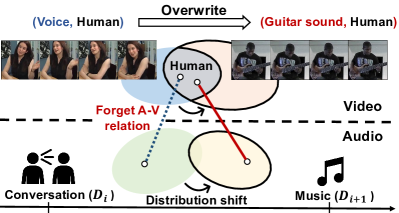
Figure 3: Challenge of multimodal correlation overwriting. Let the model be learned human voice with video frame inputs (blue). During continual pre-training, the model can encounter new semantics sharing key visual objects, humans, making the model overwrite the previously learned audio information associated with humans to a new one (i.e., guitar) (red), resulting in forgetting.

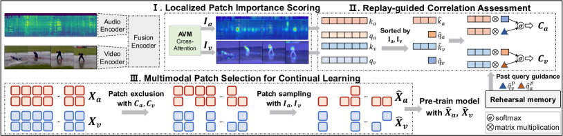
Figure 4: Overview of our approach. Our method harnesses cross-modal attention maps from the AVM module to compute importance scores in order to identify highly correlated patches (Localized Patch Importane Scoring). Comparing the attention maps created by the current queries with those generated by past queries, we compute correlation scores of the current patches with the past data (Replay-guided Correlation Assessment). Finally, we perform a probabilistic patch selection, combining the importance scores and correlation scores to select patches for continual audio-video pre-training (Multimodal Patch Selection for Continual Learning).

In this section, we delve into two key challenges in continual audio-video pre-training: 1) sparse spatio-temporal correlation 2) multimodal correlation overwriting. In Fig. 2 (b), we visualize cross-attention heat maps and observe sparse spatio-temporal correlation between the audio-video pair. Capturing highly correlated audio-video patches is crucial for understanding their semantics, allowing the model to focus on informative regions and learn complex multimodal relationships. It becomes more critical in continual audio-video pre-training methods in view of rehearsal memory. They contain a small-sized rehearsal memory designed to store key information for past tasks during continual pre-training. As rehearsal memory is limited in capacity, it’s important to store meaningful data/feature audio-video pairs associated with their semantics.

We also observe that the model forgets previously learned audio-video correlations after learning a sequence of tasks (Fig. 2 (c)). In continual audio-video pre-training, the biased data distribution poses a risk of overwriting previous multimodal correlations, driven by the close correlation between current video and past audio data, and vice versa. For instance, transitioning from a past task involving human-conversational data to a current task featuring human-playing-musical-instrument data (Fig. 3) weakens the audio-video correlations of human visuals and voices from the past task. Instead, the model potentially associates human visuals with musical sounds prevalent in the biased current data distribution, leading to the forgetting of the past human-voice relationships. This challenge, termed multimodal correlation overwriting, underscores the critical need to identify data regions with high correlation to past steps.

4 Continual Audio-Video Pre-training with Spatio-Temporal Localized Alignment

To overcome critical challenges in earlier sections, we introduce a novel continual audio-video pre-training approach, dubbed Spatio-TEmporal LocaLized Alignment (STELLA), illustrated in Fig. 4. We first propose a lightweight trainable module that determines importance scores, guiding the model to focus on spatio-temporally aligned audio-visual regions (Sec. 4.1). Next, we introduce a unique process of assessing multimodal correlations between current and previous steps to compute correlation scores, identifying patches having higher correlations to the past steps (Sec. 4.2). Finally, we describe the probabilistic patch selection framework, which uses the importance and correlation scores to select audio and video patches for continual pre-training (Sec. 4.3). Please see Algo. 1 for a detailed training process.

4.1 Localized Patch Importance Scoring

Inspired by the observation that audio-video data pairs are only correlated with a sparse spatio-temporal region, we aim to capture accurate local semantics between audio and visual cues by computing importance scores for each patch to identify a few strongly associated audio-video patches. We achieve this by introducing an Audio-Video Matching (AVM) module that maps the output embeddings of the modality encoders to queries and keys ($\bm{q},\bm{k}$) to compute attention map by $\mu(\bm{q},\bm{k})\!=\!\bm{q}\bm{k}^{\top}/\beta*\sqrt{d}$, where $\beta$ denotes a temperature coefficient. Due to a page limit, please see Sec. D for the detailed architecture of the AVM module. Given $(X_{a},X_{v})$, we first map audio/video patches using the modality encoders and the AVM module to queries and keys $(\bm{q}_{a},\bm{k}_{a})\!\in\!\mathbb{R}^{B\!\times\!H\!\times\!M\!\times\!D}$, $(\bm{q}_{v},\bm{k}_{v})\!\in\!\mathbb{R}^{B\!\times\!H\!\times\!N\!\times\!D}$, where $H$ is the number of heads and $D$ is the dimension size. Then, we generate cross-attention maps for each modality as follows:

$$\small\begin{split}\bm{A}_{a}\!=\!\mu(\bm{q}_{v},\bm{k}_{a}),\;\bm{A}_{v}\!=\!\mu(\bm{q}_{a},\bm{k}_{v}),\end{split}$$ (1)

where $\bm{A}_{a}\!\in\!\mathbb{R}^{B\!\times\!H\!\times\!N\!\times\!M}$, and $\bm{A}_{v}\!\in\!\mathbb{R}^{B\!\times\!H\!\times\!M\!\times\!N}$. Then, we compute the importance scores $\bm{I}_{a}\!\in\!\mathbb{R}^{B\!\times\!M}$, and $\bm{I}_{v}\!\in\!\mathbb{R}^{B\!\times\!N}$ by applying Softmax normalization on the last dimension:

$$\small\begin{split}\bm{I}_{a}&=\texttt{MeanPool}\left(\texttt{Softmax}\left(\bm{A}_{a}\right)\right),\\ \bm{I}_{v}&=\texttt{MeanPool}\left(\texttt{Softmax}\left(\bm{A}_{v}\right)\right).\end{split}$$ (2)

The importance score represents the average correlation between an audio (or a video) patch and the paired modality patches. That is, the higher value in $\bm{I}$ indicates the higher importance of the corresponding patch in view of the opposite modality (A$\leftrightarrow$V), thus helping the model to select locally aligned audio-video patches in Sec. 4.3.

4.2 Replay-guided Correlation Assessment

To tackle the challenge of multimodal correlation overwriting, the model requires a careful balance between retaining previous knowledge and adapting new one. Thus, we propose to compare cross-attention maps activated by current and past queries to assess relative multimodal correlation and exclude patches exhibiting higher correlation to the past steps. Our ultimate goal is to select $\kappa_{a}$ audio and $\kappa_{v}$ video patches where $\kappa_{a}=M\cdot\rho_{a}$ and $\kappa_{v}=N\cdot\rho_{v}$, with $\rho_{a}$ and $\rho_{v}$ denoting sampling ratios for audio and video. To this end, we obtain locally aligned queries $\widehat{\bm{q}}_{a},\widehat{\bm{q}}_{v}\!\in\!\mathbb{R}^{B\!\times\!H\!\times\!D}$ and keys $\widehat{\bm{k}}_{a}\!\in\!\mathbb{R}^{B\!\times\!H\!\times\!\kappa_{a}\!\times\!D},\widehat{\bm{k}}_{v}\!\in\!\mathbb{R}^{B\!\times\!H\!\times\!\kappa_{v}\!\times\!D}$ using the indices sorted in ascending order based on the importance scores $\bm{S}_{a}\!=\!\texttt{argsort}(\bm{I}_{a})$, $\bm{S}_{v}\!=\!\texttt{argsort}(\bm{I}_{v})$:

$$\small\begin{split}\widehat{\bm{q}}_{n}[i,:,j]&=\bm{q}_{n}[i,:,\bm{S}_{n}[i,j]],\;\bm{I}_{n}^{s}[i,j]=\bm{I}_{n}[i,\bm{S}_{n}[i,j]],\\ \widehat{\bm{q}}_{n}&\leftarrow\texttt{MeanPool}\left(\widehat{\bm{q}}_{n},\texttt{weight}\!=\!\bm{I}_{n}^{s}\right),\\ \widehat{\bm{k}}_{n}[i,:,j]&=\bm{k}_{n}[i,:,\bm{S}_{n}[i,j]],\;i=1,\ldots,B,\;j=1,\ldots,\kappa_{n},\end{split}$$ (3)

where $n\!\in\!(a,v)$ and $\texttt{MeanPool}\left(\cdot,\texttt{weight}\right)$ indicates weighted mean operation. We utilize the queries and keys to compute cross-attention maps $\widehat{\bm{A}}_{a}\!=\!\mu_{(}\widehat{\bm{q}}_{v},\widehat{\bm{k}}_{a})\!\in\!\mathbb{R}^{B\!\times\!H\!\times\!\kappa_{a}}$, $\widehat{\bm{A}}_{v}\!=\!\mu(\widehat{\bm{q}}_{a},\widehat{\bm{k}}_{v})\!\in\!\mathbb{R}^{B\!\times\!H\!\times\!\kappa_{v}}$. Similarly, we compute cross-attention maps $\widehat{\bm{A}}_{a}^{p}\!=\!\mu(\widehat{\bm{q}}_{v}^{p},\widehat{\bm{k}}_{a})$,$\widehat{\bm{A}}_{v}^{p}\!=\!\mu(\widehat{\bm{q}}_{a}^{p},\widehat{\bm{k}}_{v})$ by using the past queries $\widehat{\bm{q}}_{a}^{p},\;\widehat{\bm{q}}_{v}^{p}$, which were computed during the past steps and stored in the rehearsal memory. Each $\widehat{\bm{A}}$ shows how the given queries are correlated to the current patches. To assess the relative correlation between the past and current steps on the current patches, we stack the audio $(\widehat{\bm{A}}_{a},\widehat{\bm{A}}_{a}^{p})$ and video attention maps $(\widehat{\bm{A}}_{v},\widehat{\bm{A}}_{v}^{p})$, resulting in an extended last dimension, respectively. Subsequently, we apply Softmax normalization on the extended last dimension, resulting in correlation scores $\bm{C}_{a}$ and $\bm{C}_{v}$ as follows:

$$\small\begin{split}\bm{C}_{a}&=\texttt{MeanPool}\left(\texttt{Softmax}\left([\widehat{\bm{A}}_{a},\widehat{\bm{A}}_{a}^{p}]\right)\right),\\ \bm{C}_{v}&=\texttt{MeanPool}\left(\texttt{Softmax}\left([\widehat{\bm{A}}_{v},\widehat{\bm{A}}_{v}^{p}]\right)\right).\end{split}$$ (4)

Each value in the correlation score moves closer to one when the corresponding patch exhibits a higher multimodal correlation with the opposite modality data from the past steps compared to the correlation with its modality pair. Hence, patches with high $\bm{C}$ values should more likely be excluded to preserve previously learned multimodal correlations.

4.3 Multimodal Patch Selection for Continual Learning

Leveraging the importance score $\bm{I}_{v}$ and correlation score $\bm{C}_{v}$, we enhance multimodal alignment and stability of the continual pre-training by sorting video patch indices. Initially, a Bernoulli distribution on $\bm{C}_{v}$ produces $\bm{F}_{v}$. True values in $\bm{F}_{v}$ indicate that the corresponding patches are chosen to be excluded. Hence, we zero out elements in $\bm{I}_{v}$ aligned with the True values in $\bm{F}_{v}$ to create $\tilde{\bm{I}}_{v}$. Subsequently, applying a multinomial probability distribution to $\tilde{\bm{I}}_{v}$ yields the informative video patch indices $\tilde{\bm{S}}_{v}\in\mathbb{R}^{B\!\times\!N}$:

$$\small\begin{split}\tilde{\bm{I}}_{v}[i,j]&=\begin{cases}0&\text{if }\bm{F}_{v}[i,j]\;\;\;i\!=\!1,\ldots,B\\ \bm{I}_{v}[i,j]&\text{otherwise}\;\;\;j\!=1,\ldots,N,\end{cases}\\ \tilde{\bm{S}}_{v}&=\texttt{Multinomial}\left(\tilde{\bm{I}}_{v},\right).\end{split}$$ (5)

Similarly, we utilize the importance score $\bm{I}_{a}$ and correlation score $\bm{C}_{a}$ to generate the informative audio patch indices. To preserve the local correlation among audio patches by temporal continuity, we segment $\bm{I}_{a}$ into time chunks. To this end, we reshape the importance score $\bm{I}_{a}$ into a time-frequency dimension, average along the frequency dimension, and split the time dimension with time chunk size $\bm{L}_{c}$. This operation yields $\bm{I}^{c}_{a}\!\in\!\mathbb{R}^{B\!\times\!\left|t/p\right|/\left|\bm{L}_{c}\right|}$, which indicates the importance of audio time chunks. For $\bm{C}_{a}$, we apply Bernoulli probability distribution to generate $\bm{F}_{a}$.

We select informative time chunks with high $\bm{I}^{c}_{a}$ values while excluding the indices aligned with True values in $\bm{F}_{a}$ to generate the informative audio patch indices $\tilde{\bm{S}}_{a}\in\mathbb{R}^{B\!\times\!M}$. The detailed steps of audio patch selection are in  Algo. 2.

Algorithm 1 Continual Pre-training of STELLA

0:  Dataset $\mathcal{D}_{i}$, model $f_{\theta,i-1}$, AVM module $h_{\Theta,i-1}$, rehearsal memory $\mathcal{M}$.

1:  for batch $(X_{a},\;X_{v})\sim\mathcal{D}_{i}$ do

2:     $\bm{k}_{a},\bm{q}_{a},\bm{A}_{a},\;\bm{k}_{v},\bm{q}_{v},\bm{A}_{v}\leftarrow\textsc{AVM}(X_{a},\;X_{v})$ COMMENT$\rhd$ Eq. 1

3:     $\bm{I}_{a},\;\bm{I}_{v}\leftarrow\textsc{Importance}(\bm{A}_{a},\;\bm{A}_{v})$ COMMENT$\rhd$ Eq. 2

4:     $\widehat{\bm{k}}_{a},\widehat{\bm{q}}_{a},\;\widehat{\bm{k}}_{v},\widehat{\bm{q}}_{v}\leftarrow\textsc{Sort}(\bm{k}_{a},\bm{q}_{a},\bm{I}_{a},\bm{k}_{v},\bm{q}_{v},\bm{I}_{v})$ COMMENT$\rhd$ Eq. 3

5:     $X_{a}^{p},X_{v}^{p},\;\widehat{\bm{q}}_{a}^{p},\widehat{\bm{q}}_{v}^{p},\;\bm{I}_{a}^{p},\bm{I}_{v}^{p},\;\bm{C}_{a}^{p},\bm{C}_{v}^{p}\leftarrow\mathcal{M}$

6:     $\bm{C}_{a},\;\bm{C}_{v}\leftarrow\textsc{Compare}(\widehat{\bm{k}}_{a},\widehat{\bm{q}}_{v},\widehat{\bm{q}}_{v}^{p},\;\widehat{\bm{k}}_{v},\widehat{\bm{q}}_{a},\widehat{\bm{q}}_{a}^{p})$ COMMENT$\rhd$ Eq. 4

7:     $\widehat{X}_{a},\widehat{X}_{a}^{p}\leftarrow\textsc{Pick}([X_{a},X_{a}^{p}],[\bm{I}_{a},\bm{I}_{a}^{p}],[\bm{C}_{a},\bm{C}_{a}^{p}])$

8:     $\widehat{X}_{v},\widehat{X}_{v}^{p}\leftarrow\textsc{Pick}([X_{v},X_{v}^{p}],[\bm{I}_{v},\bm{I}_{v}^{p}],[\bm{C}_{v},\bm{C}_{v}^{p}])$ COMMENT$\rhd$ Eq. 6

9:     $\mathcal{M}\leftarrow\mathcal{M}\cup\left(X_{a},X_{v},\;\widehat{\bm{q}}_{a},\widehat{\bm{q}}_{v},\;\bm{I}_{a},\bm{I}_{v},\;\bm{C}_{a},\bm{C}_{v}\right)$

10:     $\Theta\leftarrow\Theta-\eta\nabla h_{\Theta,i-1}\left(X_{a},\;X_{v}\right)$

11:     $\theta\leftarrow\theta-\eta\nabla f_{\theta,i-1}\left([\widehat{X}_{a},\widehat{X}_{a}^{p}],\;[\widehat{X}_{v},\widehat{X}_{v}^{p}]\right)$

12:  end for

Finally, based on $\tilde{\bm{S}}_{a},\tilde{\bm{S}}_{v}$, we select $\kappa_{a},\kappa_{v}$ of audio, video patches to form new input $(\widehat{X}_{a},\widehat{X}_{v})$. Substituting $(X_{a},X_{v})$ into $(\widehat{X}_{a},\widehat{X}_{v})$ enables the model to effectively learn new audio-video relationships while preserving previously learned ones with enhanced efficiency. The final patch selection is performed as follows:

$$\small\begin{split}\widehat{X}_{n}[i,j]&=X_{n}[i,\tilde{\bm{S}}_{n}[i,j]],\;i=1,\ldots,B,\;j=1,\ldots,\kappa_{n},\end{split}$$ (6)

where $n\!\in\!(a,v)$. With the selected patches, we perform continual pre-training based on the DER++ framework with the penalty loss ($\ell^{p}$), which encourages the model to maintain the features of the rehearsal memory to mitigate their drifts. Hence, our final pre-training objective is $\mathcal{L}=\ell^{r}+\lambda\ell^{c}+\alpha\ell^{p}$, where $\alpha$ is a hyperparameter for the penalty loss.

Efficient rehearsal memory usage is crucial especially in continual audio-video learning scenarios due to the large video sizes. The effective storage of past data can notably augment the diversity of data within the memory. To address this, we propose STELLA+, an extension of STELLA, where memory stores the selected patches instead of raw data (Algo. 3). The introduction of STELLA+ represents a distinct and complementary direction to STELLA, demonstrating the efficacy of efficient memory utilization.

Table 1: Results of audiovisual zero-shot retrieval task on Continual-VS and Continual-AS. R@K means top-K recall. The results are the means of 3 independent runs. The best and the second best results are highlighted in bold and underline, respectively.

		Continual-VS								Continual-AS
	Method	R@1		R@5		R@10		Avg		R@1		R@5		R@10		Avg
		$\mathcal{A}\uparrow$	$\mathcal{F}\downarrow$	$\mathcal{A}\uparrow$	$\mathcal{F}\downarrow$	$\mathcal{A}\uparrow$	$\mathcal{F}\downarrow$	$\mathcal{A}\uparrow$	$\mathcal{F}\downarrow$	$\mathcal{A}\uparrow$	$\mathcal{F}\downarrow$	$\mathcal{A}\uparrow$	$\mathcal{F}\downarrow$	$\mathcal{A}\uparrow$	$\mathcal{F}\downarrow$	$\mathcal{A}\uparrow$	$\mathcal{F}\downarrow$
Audio-to-Video	Finetune	0.98	4.16	3.75	11.98	6.17	15.35	3.63	10.50	1.48	2.90	3.84	11.34	5.41	17.83	3.58	10.69
	ER	4.09	3.66	11.66	9.17	17.78	10.20	11.18	7.68	4.94	2.97	12.33	7.46	17.60	11.17	11.62	7.20
	MIR	4.59	3.14	12.26	8.34	17.51	11.17	11.45	7.55	5.21	2.93	13.16	7.10	18.04	9.14	12.14	6.39
	DER++	4.03	3.62	13.74	6.31	19.79	7.11	12.52	5.68	4.51	3.75	12.15	8.42	16.85	11.86	11.17	8.01
	GMED	4.17	2.73	12.01	6.84	18.95	6.33	11.71	5.30	4.71	2.27	12.83	7.45	18.44	9.18	11.99	6.30
	CLS-ER	4.61	3.20	14.07	6.77	19.54	8.92	12.74	6.30	4.17	4.50	11.28	11.06	16.85	12.55	10.77	9.37
	LUMP	3.56	2.79	11.68	7.65	17.40	8.52	10.88	6.32	3.73	3.03	13.74	5.29	19.50	8.17	12.32	5.50
	ESMER	4.51	3.68	14.98	6.22	21.25	7.50	13.58	5.80	5.18	4.92	14.14	9.19	18.69	12.84	12.67	8.98
	STELLA (Ours)	5.34	2.04	15.04	5.20	22.10	5.90	14.16	4.38	5.22	2.26	13.09	7.95	18.75	10.65	12.35	6.95
	STELLA+ (Ours)	5.39	2.71	16.76	5.15	24.18	5.99	15.44	4.62	5.36	4.24	16.76	5.54	23.65	7.44	15.26	5.74
	Multitask	6.45	$-$	20.19	$-$	29.01	$-$	18.55	$-$	8.28	$-$	24.14	$-$	33.74	$-$	22.05	$-$
Video-to-Audio	Finetune	1.22	4.47	4.17	11.23	6.95	14.67	4.11	10.12	1.50	3.23	4.08	10.04	6.33	14.43	3.97	9.23
	ER	3.28	3.94	11.30	8.86	16.40	11.37	10.33	8.06	3.70	4.36	10.76	10.34	15.68	15.06	10.05	9.92
	MIR	3.54	3.47	11.82	9.11	16.69	12.90	10.68	8.49	4.26	4.59	11.29	9.87	15.97	13.73	10.51	9.40
	DER++	3.49	3.86	13.22	7.09	19.03	9.04	11.91	6.66	4.23	4.50	11.66	10.10	16.24	13.97	10.71	9.52
	GMED	3.71	2.61	11.87	6.46	17.20	9.57	10.93	6.21	3.99	4.42	10.65	10.39	15.41	14.78	10.02	9.86
	CLS-ER	4.09	3.11	13.30	6.96	19.43	9.68	12.27	6.58	4.25	4.58	9.78	11.65	13.45	17.65	9.16	11.29
	LUMP	3.24	3.30	11.02	7.55	16.91	9.13	10.39	6.66	3.13	3.91	10.60	8.63	16.02	12.26	9.92	8.27
	ESMER	4.65	2.74	14.54	6.27	20.80	8.36	13.33	5.79	4.39	4.92	11.55	12.16	16.41	16.41	10.78	11.16
	STELLA (Ours)	5.30	2.40	15.43	4.84	21.47	6.70	14.07	4.65	4.49	3.39	12.08	9.00	17.31	12.75	11.29	8.38
	STELLA+ (Ours)	5.86	1.56	17.21	4.09	23.53	6.02	15.53	3.89	5.48	4.06	15.65	7.13	22.29	8.92	14.47	6.70
	Multitask	6.85	$-$	21.93	$-$	30.63	$-$	19.80	$-$	8.05	$-$	25.81	$-$	35.60	$-$	23.15	$-$

5 Experiments

In this section, we experimentally validate the effectiveness of our method in task-free continual audio-video pre-training. We start by outlining our experimental setup in Sec. 5.1, covering datasets, evaluation methods, evaluation metrics, and baseline methods employed for our experiments. Subsequently, we present the experimental results and conduct a comprehensive analysis in Sec. 5.2.

5.1 Experimental Setup

Evaluation Protocol

We validate our method on continual audio-video pre-training over VGGSound (Chen et al., 2020) and AudioSet (Gemmeke et al., 2017) datasets, consisting of 10s videos. We split each dataset into multiple tasks based on its high-level category information. We name them as Continual-VS and Continual-AS, respectively. For evaluation, we conduct various audiovisual downstream tasks: retrieval, sound source localization, and event localization. Further details, including data split, data statistics, and downstream tasks, are provided in Sec. B.

Baselines

To quantitatively assess our method, we compare its performance with several task-free continual learning methods: ER (Rolnick et al., 2019), MIR (Aljundi et al., 2019a), DER++ (Buzzega et al., 2020), GMED (Jin et al., 2021), CLS-ER (Arani et al., 2022), LUMP (Madaan et al., 2022), and ESMER (Sarfraz et al., 2023). The details of the baseline methods are explicated in Sec. A. All methods employ reservoir sampling (Vitter, 1985) to sample past instances from the rehearsal memory for $2K$ (Continual-VS) and $5K$ (Continual-AS) instances during continual pre-training, except for STELLA+, which adjusts instance count based on sampling ratios ($\rho_{a},\rho_{v}$) to match the memory size of other methods. We additionally report the result of Finetune, the model continually pre-trained without additional methods, and Multitask, the model pre-trained with the entire datasets. They serve as lower and upper bounds, respectively, in assessing learned representation.

Evaluation Metrics

After each end of pre-training on $\mathcal{D}_{t}$, we estimate task-specific performances $\{\textit{acc}_{t,i}\}^{t}_{i=1}$, where $\textit{acc}_{t,i}$ denotes the performance of the downstream task associated with $\mathcal{D}_{i}$ when evaluated with $f_{\theta,t}$, the model pre-trained up to the $t$-th task. Here, no task boundary information is employed in performance estimation. For the evaluation, we adopt two conventional metrics in continual learning: (1) Average accuracy($\mathcal{A}$) is the mean accuracy across all tasks after the completion of pre-training on $\mathcal{D}_{\mathcal{T}}$, and it is formulated as $\mathcal{A}\!=\!\frac{1}{\mathcal{T}}\sum^{\mathcal{T}}_{i=1}\textit{acc}_{\mathcal{T},i}$. (2) Average Forgetting($\mathcal{F}$) measures the average amount of catastrophic forgetting for each task, quantified as the difference between its maximum accuracy and accuracy at the completion of pre-training on $\mathcal{D}_{\mathcal{T}}$, calculated as, $\mathcal{F}\!=\!\frac{1}{\mathcal{T}-1}\sum^{\mathcal{T}-1}_{i=1}\!\underset{t\in\{1,\ldots,\mathcal{T}-1\}}{\text{max}}\!\left(\textit{acc}_{t,i}-\textit{acc}_{\mathcal{T},i}\right)$.

5.2 Analysis for Continual Audio-Video Pre-training

STELLA achieves superior Zero-shot Audiovisual Retrieval performance compared to strong baselines. We perform audio-to-video and video-to-audio zero-shot retrieval tasks in Continual-VS and Continual-AS to quantitatively assess the learned audio-video correlation from the continual pre-training (Tab. 1). For the Continual-VS, both STELLA and STELLA+ outperform other baselines, exhibiting substantial enhancements of 0.58%p, 1.86%p and 0.74%p, 2.20%p in average audio-to-video and video-to-audio retrieval scores, respectively. In the Continual-AS, STELLA+ exhibits prominent performance advantages, with 2.59%p and 3.69%p improvements in average audio-to-video and video-to-audio retrieval scores. Notably, our methods consistently achieve high R@1 scores across all tasks. These results imply that our approach of continually pre-training on the selected patches enhances the model’s ability to comprehend the audio-video relationship by accurately capturing sparse spatio-temporal correlations. For a thorough investigation, we conduct further experiments with shuffled task orders in Sec. E. We also explore the influence of rehearsal memory size on zero-shot task performances, presenting the results in Fig. 7. Our methods consistently surpass other baselines, underscoring their effectiveness in adapting to diverse memory constraints.

STELLA is significantly efficient in terms of GPU Memory Consumption. Pre-training on the spatio-temporally aligned subset of audio-video patches also enhances efficiency. In Tab. 4, we compare GPU memory occupancy estimated across methods. STELLA consumes significantly less GPU memory than baselines, even surpassing Finetune in efficiency. Compared to DER++, STELLA achieves an efficiency gain of 43.59%. Additionally, the extra cost required in STELLA for storing the queries, importance scores, and correlation scores in the rehearsal memory is negligible (+ $0.16$ GB), based upon the fact that the size of the rehearsal memory itself is $5.47$ GB and that CLS-ER and ESMER maintain additional models, which require +$~{}1.42$ GB and +$~{}0.71$ GB additional memory, respectively.

Core components in STELLA contribute to improving evaluation performance. To validate our patch selection method, we compare our two core components with MATS (Hwang et al., 2022), an adaptive patch selection method aiming to discard redundant patches during video pre-training, and with a simple random patch selection method, denoted as Random. We decompose STELLA into Localized Patch Importance Scoring (LPIS) and Replay-guided Correlation Assessment (RCA). All the above methods follow the default sampling ratio and were built upon DER++. In Continual-VS zero-shot retrieval tasks, LPIS and RCA show competitive results against baselines including MATS and Random (Tab. 4). LPIS enhances the model’s audio-video semantics comprehension. Conversely, RCA demonstrates more robustness in forgetting but with a lower average retrieval score, indicating a need for improved guidance in understanding audio-video semantics. Combining both components, STELLA achieves improved performances, emphasizing the importance of considering both the sparse correlation and forgetting in continual audio-video pre-training.

Table 2: Efficiency analysis. GPU memory occupancy (GPU M.) is measured in GB, estimated in a V100 with a batch size of 9.

Method	A$\rightarrow$V		V$\rightarrow$A		GPU M.$\downarrow$
	$\mathcal{A}\uparrow$	$\mathcal{F}\downarrow$	$\mathcal{A}\uparrow$	$\mathcal{F}\downarrow$
Finetune	3.63	10.50	4.11	10.12	18.34
ER	11.18	7.68	10.33	8.06	30.95
MIR	11.45	7.55	10.68	8.49	31.17
DER++	12.52	5.68	11.91	6.66	30.95
GMED	11.71	5.30	10.93	6.21	32.03
CLS-ER	12.74	6.30	12.27	6.58	32.50
LUMP	10.88	6.32	10.39	6.66	18.36
ESMER	13.58	5.80	13.33	5.79	31.45
STELLA (Ours)	14.16	4.38	14.07	4.65	17.45
STELLA+ (Ours)	15.44	4.62	15.26	3.89	17.15

Table 3: Sampling methods. Experiments with various sampling methods. LPIS: Localized Patch Importance Scoring in Sec. 4.1, RCA: Replay-guided Correlation Assessment Sec. 4.2.

Method	LPIS	RCA	A$\rightarrow$V		V$\rightarrow$A		GPU M.$\downarrow$
			$\mathcal{A}\uparrow$	$\mathcal{F}\downarrow$	$\mathcal{A}\uparrow$	$\mathcal{F}\downarrow$
Random	$-$	$-$	12.64	6.46	12.55	6.58	16.63
MATS	$-$	$-$	12.91	6.55	12.70	6.80	21.30
STELLA (Ours)	$-$	$-$	12.52	5.68	11.91	6.66	30.95
	$\checkmark$	$-$	13.44	5.50	13.27	5.94	17.48
	$-$	$\checkmark$	13.40	5.30	12.94	5.44	17.48
	$\checkmark$	$\checkmark$	14.16	4.38	14.07	4.65	17.45

Table 4: MSR-VTT audiovisual retrieval. MSR-VTT audiovisual retrieval task performances. The best and the second best results are highlighted in bold and underline, respectively.

Method	A$\rightarrow$V			V$\rightarrow$A
	R@1	R@5	R@10	R@1	R@5	R@10
Finetune	1.00	4.15	6.44	1.33	3.19	6.15
ER	2.26	7.89	13.38	2.26	8.78	13.42
MIR	2.48	7.59	11.89	1.85	7.37	11.81
DER++	1.93	8.23	13.75	2.52	8.30	13.42
GMED	1.67	6.81	11.81	1.44	6.04	11.59
CLS-ER	2.15	8.45	12.93	2.15	7.63	12.82
LUMP	1.78	7.70	12.07	1.59	7.04	11.81
ESMER	2.33	8.37	13.78	2.30	8.48	13.93
STELLA (Ours)	2.70	8.70	13.96	2.67	8.81	14.30
STELLA+ (Ours)	2.37	9.11	15.07	2.44	10.14	15.62

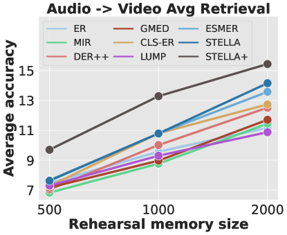
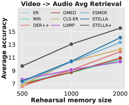
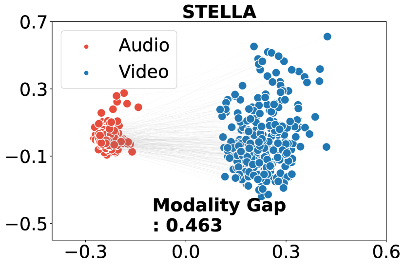
Figure 5: Downstream performance on various rehearsal memory sizes. We evaluate downstream task performances on the pre-trained models with various rehearsal memory sizes on the Continual-VS.

Figure 6: Modality gap estimation. (Left): Estimation of modality gap after the completion of each task. (Continual-VS) (Right): Visualizations of modality gap corresponding to the music task with the model pre-trained up to the last task in the Continual-VS dataset with ESMER (top) and our method (bottom).

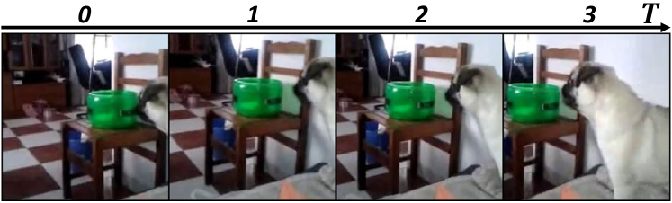
(a) Raw data

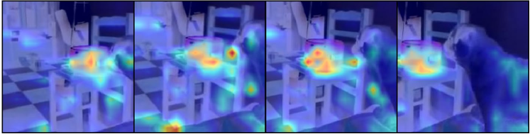
(b) Audiovisual attention (CLS-ER)

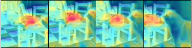
(c) Audiovisual attention (ESMER)

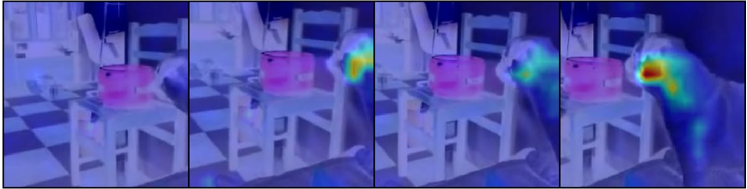
(d) Audiovisual attention (STELLA)

Figure 7: Sound source localization (a) A raw data describing a dog barking. (b)~(c): We visualize cross-attention maps using cosine similarity between each video patch and averaged audio embedding of the corresponding audio. (d): We use the AVM module in STELLA to visualize cross-attention maps. For more examples, please see Fig. 12.

STELLA excels in various audiovisual downstream tasks. To evaluate the acquired transferable knowledge through continual audio-video pre-training, we perform diverse audiovisual downstream tasks. Compared to the earlier zero-shot retrieval tasks, we use the models continually pre-trained until completion of the last task of Continaul-VS, and evaluate on different audiovisual datasets. First, we conduct audiovisual retrieval experiments on the MSR-VTT (Xu et al., 2016) dataset. We train the pre-trained models on the MSR-VTT training dataset with the training objective in Sec. 3.1 and evaluate them on the MSR-VTT test dataset. As shown in Tab. 4, our methods consistently outperform baselines, demonstrating that our methods excel at understanding relationships in audio-video pairs. Furthermore, we perform a sound source localization task on the AVE (Tian et al., 2020) dataset to evaluate the model’s ability to detect sound sources within visual scenes. In Fig. 7, given audio containing a barking dog, all methods struggle to precisely locate sound sources, concentrating on the uncorrelated object (green bottle) in the visual scene. In contrast, the AVM module in STELLA stands out by precisely identifying the correct sound source, proving its efficacy in aligning multimodal data even in continual pre-training scenarios. More audiovisual downstream task results, including event localization and retrieval tasks, are available in Sec. E.

STELLA can preserve the modality gap between audio and video embeddings even after continual learning. Recent research in multimodal learning (Liang et al., 2022) reveals that embeddings cluster by modality in representation space. Such modality-dependent clustering behavior introduces the concept of modality gap, which refers to the distance between these clusters (Fig. 7 (Right)). A larger modality gap is generally considered favorable under well-separated modality clusters since it indicates that the model can distinguish between different modalities effectively. Hence, in the context of continual audio-video pre-training, maintaining a large modality gap between the two modalities throughout tasks is desirable, as deviating from it suggests a departure from the optimal state. Hence, during continual pre-training, we estimate the modality gap at the end of each task, utilizing evaluation data of each task. The estimated modality gaps of baselines are presented in Fig. 7 (Left). Our methods consistently maintain the highest modality gap compared to other approaches. Moreover, our methods exhibit small modality gap declines, indicating that the models suffer less from the forgetting of previous multimodal correlations, which supports the validity of our approach in preventing modality correlation overwriting in Sec. 4.2 to address the issue of audio-video relation forgetting. Sec. G provides more analysis using the modality gap including Continual-AS and about two key components of our approach. Besides, some previous works (Udandarao, 2022) observe that reducing modality gaps also has benefits. Based on the modality gap analysis (Udandarao, 2022), there exists a modality gap that yields the best downstream task performances. However would like to emphasize that we use the modality to estimate the change in the modality gap throughout continual pre-training, not to find the best modality gap of the backbone model.

6 Conclusion

In this paper, we investigate the critical challenges in continual audio-video pre-training under the task-free scenario, where the model continuously learns a course of audio-video multimodal tasks sequentially and cannot access previous tasks and task oracle both on pre-training and fine-tuning. We empirically observe that the audio-video models suffer from the issue of sparse spatiotemporal correlation and representational forgetting of audio-video relationships. To overcome these limitations, we propose a novel continual audio-video multimodal pre-training method for the first time that adaptively captures sparse audio-video attention to learn accurate audio-video relationships while mitigating forgetting from previously learned relationships without requiring task identification.

Broader impact

In this work, we suggest STELLA and compare it with other recent baselines in continual audio-video pre-training scenarios. Both methods use rehearsal memories to store the subset of pre-train data from the sequence of tasks. Since the sampling process is random, all methods cannot effectively alleviate the problem of privacy issues in saving videos into the rehearsal memory. One potential way of alleviating the problem is to save the subset of audio and video patches as in STELLA+. We sincerely hope that more effective ways to solve the privacy issues in the rehearsal memory be investigated while maintaining the benefits of the rehearsal-based continual learning methods.

Appendix

Organization

The supplementary file is organized as follows: First, we explain the implementation details for our experiments in Sec. A. Then, we outline the evaluation protocol of our experiments in Sec. B. In Sec. C, we elaborate on the audio-video self-supervised objectives used for pre-training the model. Additionally, Sec. D presents a detailed account of the training procedure for the VAM module. We provide additional experimental results in Sec. E. Sec. F showcases the outcomes of our hyperparameter tuning process. Furthermore, in Sec. G, we conduct more analysis on our experimental results using the modality gap. We present PyTorch-like pseudo code for audio patch selection in Sec. H. We provide STELLA+ algorithm in Sec. I. In Sec. J we provide more examples of visualization that show challenges in audio-video lifelong pre-training. Finally, Sec. K outlines the limitations of our study.

Appendix A Implementation Details

Hyperparameter configurations.

We referred to the original papers for initial settings of hyperparameters of continual learning methods. Based on the initial settings, we tune the hyperparameters for our continual audio-video representation learning. Searched hyperparameters are listed in Tab. 5. In our method, $\alpha$ denotes a multiplier for the penalty loss to minimize the distance between obtained logits from the buffer instances and their logits stored at the past timestep. We also listed our pre-training and fine-tuning hyperparameters in Tab. 6.

Table 5: Continual learning method hyperparameters.

METHOD	Continual-VS	Continual-AS
ER	-	-
MIR	$C\;:\;5$	$C\;:\;5$
DER++	$\alpha\;:\;0.5$	$\alpha\;:\;1.0$
GMED	$\alpha\;:\;0.1\;\beta\;:\;0.05\;\gamma\;:\;1.0$	$\alpha\;:\;0.1\;\beta\;:\;0.01\;\gamma\;:\;1.0$
CLS-ER	$\lambda\;:\;0.1\;\alpha_{S}\;:\;0.999\;\alpha_{P}\;:\;0.999\;r_{S}\;:\;0.6\;r_{P}\;:\;0.8$	$\lambda\;:\;0.1\;\alpha_{S}\;:\;0.999\;\alpha_{P}\;:\;0.999\;r_{S}\;:\;0.6\;r_{P}\;:\;0.8$
LUMP	$\lambda\;:\;0.1$	$\lambda\;:\;0.05$
ESMER	$\alpha_{l}\;:\;0.99\;\beta\;:\;1.0\;\gamma\;:\;0.15\;\alpha\;:\;0.999\;r\;:\;0.2$	$\alpha_{l}\;:\;0.99\;\beta\;:\;1.0\;\gamma\;:\;0.2\;\alpha\;:\;0.999\;r\;:\;0.2$
STELLA (Ours)	$\alpha\;:\;0.5\;\beta\;:\;0.4\;\rho_{a}\;:0.5\;\rho_{v}\;:0.5$	$\alpha\;:\;0.5\;\beta\;:\;0.1\;\rho_{a}\;:0.5\;\rho_{v}\;:0.5$

Table 6: Audio-Video pre-training and fine-tuning hyperparameters.

	Pretrain		Finetune
Dataset	Continual-VS	Continual-AS	MSR-VTT	AVE
Optimizer	Adam		AdamW
Optimizer momentum	$\beta_{1},\beta_{2}=0.95,0.999$
Learning rate	1e-4			1e-3
Weight decay	5e-7			5e-6
Learning rate schedule	-		CosineScheduler
Warmup epochs	-			2
Epoch	10	15	15
Batch size	48	36	48	12
GPUs	4 A100 or 4 V100			4 Titan X Pascal
Audio Random Time Shifting	yes			no
Audio Random Noise	yes			no
Audio Norm Mean	-5.081
Audio Norm STD	4.485
Video MultiScaleCrop	yes
Video Norm Mean	[0.485, 0.456, 0.406]
Video Norm STD	[0.229, 0.224, 0.225]

Baselines.

ER (Rolnick et al., 2019) employs rehearsal memory and learns the past data in the memory during training on the current task to mitigate forgetting. All the baselines below employ the rehearsal memory to store the subset of past data. MIR (Aljundi et al., 2019a) introduces a strategy that retrieves data the model is likely to forget during the current task and trains the model with the retrieved data. To retrieve the data, it pseudo-updates the model with the data in the current step and finds the mini-batch of past data that gives the highest training loss. DER++ (Buzzega et al., 2020) matches stored logits in the rehearsal memory from past tasks with the current ones, ensuring a smoother transition and preventing abrupt changes in the logits during training. In our setting, we store both audio and video logits in the rehearsal memory and apply the method independently. GMED (Jin et al., 2021) tackles forgetting by using gradient information to update past data in the rehearsal memory. The data is updated to maximize interference of the current task to help the model retain past knowledge. Hence, it virtually updates the model with data from the current step and calculates the relative gradient by the past data to update the past data. CLS-ER (Arani et al., 2022) draws inspiration from the complementary learning system theory and maintains two models to retain short-term memories and long-term memories; one quickly adapts to new tasks and the other is slowly updated to retrain past knowledge. The slowly updated model transfers retained knowledge to the adaptable one, ensuring the retention of past information. LUMP (Madaan et al., 2022) integrates past and current data by mixing the two data, rather than replaying the past data together with data from the current task to handle the forgetting issue. In our setting, we integrate the past and current video and audio respectively with the same ratio. Lastly, ESMER (Sarfraz et al., 2023) employs a semantic memory model that has the same structure as the pre-trained model to slowly integrate the knowledge encoded in the weights. It refers to the memory model to alleviate the effect of the data from the current batch that induces abrupt drift in the learned representations in order to reduce forgetting. The suggested method effectively handles the abrupt representation changes when the data distribution shifts.

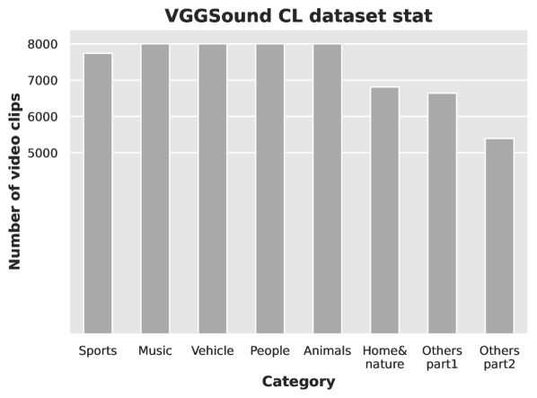
(a) Continual-VS statistics

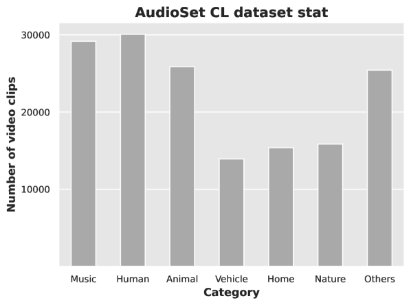
(b) Continual-AS statistics

Figure 8: Stastics of Audio-Video datasets (a): We split the VGGSound into 8 tasks, where each subset dataset consists of similar amounts of video clips. (b): We split the AudioSet into 7 tasks. Unlike the VGGSound dataset, the number of video clips varies significantly for each task.

Appendix B Continual pre-training evaluation protocol

Audiovisual Dataset Configuration

In this section, we specify how we design our continual audio-video pre-training experiments using two benchmark datasets: VGGSound and AudioSet. To mimic the data distribution shift due to the new audio-video semantics described in Sec. 1, we split the dataset according to the high-level categories. For the VGGSound dataset, we split the dataset into eight tasks based on the category labels (Chen et al., 2020). Each task dataset consists of 6k-8k video clips from 20 different classes as in Fig. 8 (a). We name it as Continual-VS. Then, we construct another pre-training dataset by combining the unused training dataset in VGGSound with the AudioSet-20k (Gemmeke et al., 2017), resulting in a total of 104k video clips. We took care to exclude the unused VGGSound video samples whose class labels are present in the Continual-VS. Using the merged dataset, we pre-train the backbone weights before continual pre-training. This ensures that the model does not underperform at the initial continual pre-training stages while the model does not acquire any task-specific knowledge at the beginning. For the Continual-VS continual pre-training, we follow the task sequence: sports$\rightarrow$music$\rightarrow$vehicle$\rightarrow$people$\rightarrow$animals$\rightarrow$home&nature$\rightarrow$others part1(tools&others)$\rightarrow$others part2(remaining others).

Similarly, we divided the AudioSet dataset into seven tasks, following class hierarchy information (Gemmeke et al., 2017). We name it as Continual-AS. Compared to Continual-VS, it exhibits imbalanced dataset size among tasks and contains much larger clips. To ensure proper pre-training for the Continual-AS experiments, we pre-train the model with the entire VGGSound dataset to avoid any potential performance issues during the initial stages of continual pre-training. We randomly shuffle the pre-train order and follow the task sequence: human$\rightarrow$vehicle$\rightarrow$nature$\rightarrow$animal$\rightarrow$others$\rightarrow$home$\rightarrow$music.

For downstream tasks, we use two audiovisual datasets: MSR-VTT (Xu et al., 2016) and AVE (Tian et al., 2020). MRS-VTT consists of 10,000 video clips from 20 different categories. We collect video clips that contain audio modality on both the training dataset and the test dataset. This yields $\sim 6k$ and $\sim 0.9k$ video clips, respectively. We finetune the continually pre-trained models on the MSR-VTT training dataset and evaluate on the test dataset to perform audiovisual bi-directional retrieval tasks. In the case of the AVE dataset, it contains 4143 videos with 28 different event categories. Since the dataset is a subset of AudioSet, we conduct experiments on the pre-trained models on Continaul-VS only. With this dataset, we perform two downstream tasks: sound source localization, which requires the models to locate the sounding objects in the visual scene, and audiovisual event localization, which asks the model to classify audiovisual events for each time step. Given that all the downstream task datasets represent unseen data for the pre-trained models, they allow us to gauge the extent to which the model has acquired general knowledge of audio-video correlations during continual audio-video pre-training.

Comparison between supervised continual learning setup and continual pre-training setup

To clarify our continual audio-video pre-training setup, we compare the conventional supervised continual learning with our setting as shown in Fig. 9. The supervised continual learning (Pian et al., 2023; Mo et al., 2023) revolves around updating a model based on new tasks that introduce unseen classes or domains while ensuring the preservation of past knowledge within the model. This adaptation requires human-annotated labels, but acquiring high-quality human annotations is expensive and not scalable to large datasets.

Conversely, continual pre-training (Madaan et al., 2022)(Yan et al., 2022) focuses on adapting new representations from new datasets with altered data distributions while maintaining the learned representations from previous tasks. Notably, this approach doesn’t rely on human-annotated information. In our specific scenario, we align with the principles of continual pre-training. Our evaluation process involves subjecting the continually pre-trained models to various downstream tasks, as illustrated on the right side of Fig. 9. This approach allows for a quantitative assessment of the acquired representations.

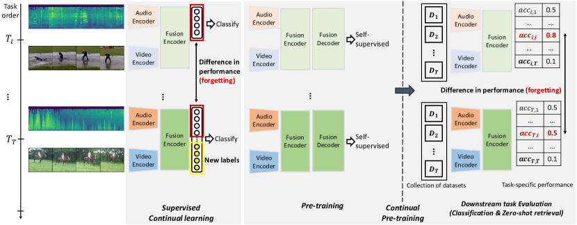
Figure 9: Comparison with supervised continual learning and continual pre-training: We illustrate the difference between the supervised continual learning setup and the continual pre-training setup that we used in our experiments.

Audiovisual downstream task configuration

When constructing audiovisual zero-shot retrieval tasks for model performance evaluation, we refer to the CAV (Gong et al., 2023) for both the Continual-VS and Continual-AS experiments. We employ the zero-shot retrieval task in CAV, but exclude evaluation samples that belong to the classes that are not included in any of the tasks. In the audiovisual event localization task, we follow experimental setups in (Lin et al., 2023). In the fine-tuning stage of the retrieval and event localization task, we freeze the backbone model, connect it to a randomly initialized trainable linear classifier, and train the classifier with the training dataset to evaluate the acquired representation.

Appendix C Audio-Video Self-supervised objectives

Given audio-video data $(X_{a},X_{v})$, we obtain $D$-dimensional embedding patches $\bm{a}$ and $\bm{v}$ as follows:

$$\small\begin{split}\bm{a}&=\texttt{Conv2d}\left(X_{a},\bm{w}_{a}\right),~{}~{}\bm{v}=\texttt{Conv2d}\left(X_{v},\bm{w}_{v}\right),\end{split}$$ (7)

where $\bm{w}_{a},\bm{w}_{v}$ denote the weights of convolutional layers, $\bm{a}\in\mathbb{R}^{B\!\times\!M\!\times\!D}$, and $\bm{v}\in\mathbb{R}^{B\!\times\!N\!\times\!D}$.

The backbone Transformer consists of an audio encoder ($E_{a}(\cdot)$), a video encoder ($E_{v}(\cdot)$), a multimodal fusion encoder ($E_{f}(\cdot)$), and a decoder ($D(\cdot)$). Then we pre-train the model by minimizing the mask reconstruction loss $\ell^{r}$:

$$\small\begin{split}&\tilde{\bm{a}},~{}\tilde{\bm{v}}=E_{f}\left(E_{a}\left(\bm{m}_{a}\otimes\bm{a}\right),~{}E_{v}\left(\bm{m}_{v}\otimes\bm{v}\right)\right),\\ &\ell^{r}=\ell^{r}_{a}+\ell^{r}_{v}=\frac{1}{B}\sum^{B}_{i=1}\left[\frac{\left(D\left(\tilde{\bm{a}}_{i}\right)-\bm{m}_{a,i}\otimes X_{a,i}\right)^{2}}{|\bm{m}_{a,i}|}+\frac{\left(D\left(\tilde{\bm{v}}_{i}\right)-\bm{m}_{v,i}\otimes X_{v,i}\right)^{2}}{|\bm{m}_{v,i}|}\right].\end{split}$$ (8)

where $\otimes$ denotes vector-matrix multiplication while preserving the input’s dimensionality. Random audio $\bm{m}_{a}$ and video mask $\bm{m}_{v}$ are drawn by a binary distribution. In this paper, we set a probability of $0.8$ for masking, consistent with (Huang et al., 2022a). Using the unmasked patches, we aim to learn the model to reconstruct the masked audio and video patches.

In addition, we also minimize masked contrastive loss to learn the semantic relationship between audio and video representation pairs by pulling those that share the same semantics while pushing the others. Following by (Gong et al., 2023), we pass the masked input patches to audio and video encoders, and subsequently map obtained features (i.e., outputs) to the fusion encoder with modality-specific layer normalization for the masked contrastive learning:

$$\small\begin{split}&\bm{c}_{a}=\texttt{MeanPool}\left(E_{f}\left(E_{a}\left(\bm{m}_{a}\otimes\bm{a}\right),LN_{a}\right)\right),\;\;\bm{c}_{v}=\texttt{MeanPool}\left(E_{f}\left(E_{v}\left(\bm{m}_{v}\otimes\bm{v}\right),LN_{v}\right)\right),\\ &\ell^{c}=-\frac{1}{B}\sum^{B}_{i=1}\left[\texttt{log}\left(\frac{\texttt{exp}(\bm{c}_{a,i}^{\top}\bm{c}_{v,i}/\tau)}{\sum^{B}_{j=1}\texttt{exp}(\bm{c}_{a,i}^{\top}\bm{c}_{v,j}/\tau)}\right)+\texttt{log}\left(\frac{\texttt{exp}(\bm{c}_{v,i}^{\top}\bm{c}_{a,i}/\tau)}{\sum^{B}_{j=1}\texttt{exp}(\bm{c}_{v,i}^{\top}\bm{c}_{a,j}/\tau)}\right)\right]\end{split}$$ (9)

, where $\tau$ is temperature hyperparameter, and $LN_{a}$ and $LN_{v}$ indicate modality-specific layer normalization for audio and video each.

Appendix D Training of Audio-Video Matching module

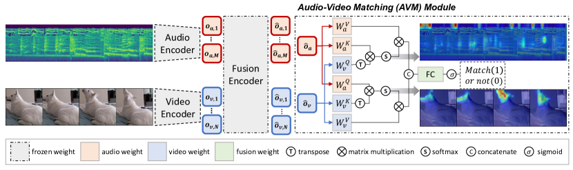
Figure 10: Overview of AVM module: The AVM (Audio-Visual Matching) module is self-supervised with the audio-video matching objective. It classifies if the given audio-video pair is positive(audio and video are from the same video) or negative(audio and video are from different videos).

AVM training procedure.

In the following section, we describe the training process of the AVM module, as illustrated in Fig. 10. Given audio-video patch pairs $(\bm{a},\bm{v})$ with the batch size of $B$, we propagate patch inputs to the frozen encoder for each modality and obtain audio-video representation pairs $(\bm{o}_{a},\bm{o}_{v})$. In order to update the module to capture the multimodal correlation between audio and its video pair, we randomly split them into positive and negative pairs, where we construct negative pairs by randomly shuffling the audio patches to pair with unmatched video patches. Next, we project the obtained positive and negative pairs into fusion space $(\bm{\tilde{o}}_{a},\;\bm{\tilde{o}}_{v})$ through the fusion encoder. Subsequently, the input pairs are fed into the AVM module. They are projected to keys, queries, and values for the cross-attention operation, by passing through trainable projection layers. The above process can be summarized as follows:

$$\small\begin{split}\bm{o}_{a},\bm{o}_{v}\!=\!E_{a}(\bm{a}),E_{v}(\bm{v})&,\;\;~{}\bm{\tilde{o}}_{a},\bm{\tilde{o}}_{v}\!=\!E_{f}(\bm{o}_{a},\bm{o}_{v})\\ \bm{q}_{a}\!=\!\bm{\tilde{o}}_{a}{\mathcal{W}}^{Q}_{a},\;\bm{k}_{a}\!=\!\bm{\tilde{o}}_{a}{\mathcal{W}}^{K}_{a},\;\bm{v}_{a}\!=\!\bm{\tilde{o}}_{a}{\mathcal{W}}^{V}_{a}&,\;\;~{}\bm{q}_{v}\!=\!\bm{\tilde{o}}_{v}{\mathcal{W}}^{Q}_{v},\;\bm{k}_{v}\!=\!\bm{\tilde{o}}_{v}{\mathcal{W}}^{K}_{v},\;\bm{v}_{v}\!=\!\bm{\tilde{o}}_{v}{\mathcal{W}}^{K}_{v},\\ \bm{A}_{a}\!=\!\texttt{Softmax}\left(\mu(\bm{q}_{v},\bm{k}_{a},\beta\!=\!1)\right)&,\;\;~{}\bm{A}_{v}\!=\!\texttt{Softmax}\left(\mu(\bm{q}_{a},\bm{k}_{v},\beta\!=\!1)\right),\\ \bm{V}_{a}\!=\!\bm{A}_{a}\bm{v}_{a}&,\;\;~{}\bm{V}_{v}\!=\!\bm{A}_{v}\bm{v}_{v}\end{split}$$ (10)

where the projections ${\mathcal{W}}^{Q}_{a},\,{\mathcal{W}}^{K}_{a},\,{\mathcal{W}}^{V}_{a},\,{\mathcal{W}}^{Q}_{v},\,{\mathcal{W}}^{K}_{v},\,{\mathcal{W}}^{V}_{v}\!\in\!\mathbb{R}^{D\!\times\!H\!\times\!d}$ are trainable parameter matrices; $D\!=\!H*d$. $\bm{V}_{a}\!\in\!\mathbb{R}^{B\!\times\!H\!\times\!N\!\times\!D},\;\bm{V}_{v}\!\in\!\mathbb{R}^{B\!\times\!H\!\times\!M\!\times\!D}$ are values highlighted by the cross-attention maps.

Next, we average the values head-wise and patch-wise, and concatenate the resulting two values into $\bm{va}\!\in\!\mathbb{R}^{B\!\times\!2D}$ in order to merge the multimodal information. Then it is passed to fully connected (FC) layers, which serve as the classification head. These FC layers take $\bm{va}$ as input, generating a vector $\hat{\bm{y}}\!\in\!\mathbb{R}^{B}$ that predicts whether each input pair corresponds to a negative of positive pair. For training the AVM module, we employ the binary cross-entropy loss to classify audio-video pairs, i.e.,

$$\begin{split}\widehat{\bm{V}}_{av}&=\texttt{Concat}\left(\texttt{MeanPool}\left(\bm{V}_{a}\right),\texttt{MeanPool}\left(\bm{V}_{v}\right)\right),\\ \widehat{\bm{y}}&=\texttt{Sigmoid}\left(\texttt{FC}(\widehat{\bm{V}}_{av})\right),~{}\mathcal{L}^{avm}=-\bm{y}\left(\texttt{log}(\widehat{\bm{y}})\right),\end{split}$$ (11)

Here, $\bm{y}\!=\!\{0,1\}^{B}$ represents ground truth labels, with $\bm{y}_{i}$ taking the value 0 when the $i\-th$ input audio-video pair is a negative pair and 1 otherwise. We pre-train the AVM module along with the backbone model. During the weight update process in the AVM module, the gradient computed from the audio-video matching objective does not propagate through the backbone encoder. This design choice ensures exploiting the AVM at a low cost. Moreover, the AVM only increases 3.18% of the total backbone model size (707.8 MB), which is efficient compared to methods like CLS-ER or ESMER which require additional backbones during training.

Appendix E Additional Experimental Results

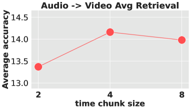
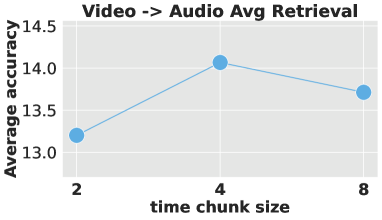
(a) Time chunk sizes

Method	A$\rightarrow$V		V$\rightarrow$A
	$\mathcal{A}\uparrow$	$\mathcal{F}\downarrow$	$\mathcal{A}\uparrow$	$\mathcal{F}\downarrow$
Frequency	13.42	5.51	12.76	6.40
No constraint	12.67	6.55	12.78	6.61
Time	14.16	4.38	14.07	4.65

(b) Audio selection methods

Figure 11: Variation of audio patch selection. (a): Average retrieval task performance on various time chunk sizes. (b): Average retrieval task performance on various audio selection methods.

Table 7: Results of audiovisual zero-shot retrieval task on Continual-VS and Continual-AS. We randomly shuffle the task sequences for continual pre-training. For the Continual-VS, we follow the task order: music $\rightarrow$ others part1 $\rightarrow$ home&nature $\rightarrow$ sports $\rightarrow$ others part2 $\rightarrow$ vehicle $\rightarrow$ animals $\rightarrow$ people. For the Continual-AS, we follow the task order: nature $\rightarrow$ human $\rightarrow$ home $\rightarrow$ vehicle $\rightarrow$ music $\rightarrow$ animal $\rightarrow$ others. R@K means top-K recall. The results are the means of 3 independent runs. The best and the second best results are highlighted in bold and underline, respectively.

		Continual-VS								Continual-AS
	Method	R@1		R@5		R@10		Avg		R@1		R@5		R@10		Avg
		$\mathcal{A}\uparrow$	$\mathcal{F}\downarrow$	$\mathcal{A}\uparrow$	$\mathcal{F}\downarrow$	$\mathcal{A}\uparrow$	$\mathcal{F}\downarrow$	$\mathcal{A}\uparrow$	$\mathcal{F}\downarrow$	$\mathcal{A}\uparrow$	$\mathcal{F}\downarrow$	$\mathcal{A}\uparrow$	$\mathcal{F}\downarrow$	$\mathcal{A}\uparrow$	$\mathcal{F}\downarrow$	$\mathcal{A}\uparrow$	$\mathcal{F}\downarrow$
Audio-to-Video	Finetune	0.80	4.15	2.96	12.23	5.05	16.91	2.94	11.10	1.50	4.72	5.49	10.41	9.80	11.91	5.60	9.01
	ER	3.89	3.06	12.10	6.55	18.30	7.74	11.43	5.78	4.52	3.16	12.72	6.93	18.83	8.00	12.02	6.03
	MIR	4.02	2.97	12.54	6.16	17.99	8.09	11.52	5.74	4.69	2.95	13.22	6.50	18.98	8.81	12.30	6.09
	DER++	4.23	3.35	12.92	7.31	18.62	9.45	11.92	6.70	4.32	4.27	12.29	8.46	18.74	10.18	11.78	7.64
	GMED	3.90	2.94	11.51	7.41	17.65	8.87	11.02	6.41	4.70	2.48	12.56	4.55	18.62	5.05	11.96	4.03
	CLS-ER	3.94	3.35	12.96	7.19	18.09	10.66	11.66	7.07	5.16	2.97	14.33	6.88	20.24	8.74	13.24	6.20
	LUMP	4.06	2.18	13.21	4.66	19.34	5.58	12.20	4.14	4.45	3.40	13.05	6.25	19.45	7.28	12.32	5.64
	ESMER	4.38	3.36	13.31	8.28	19.39	9.20	12.36	6.95	5.43	3.85	15.81	6.20	21.40	8.81	14.21	6.29
	STELLA (Ours)	4.72	2.89	14.17	5.74	19.94	5.74	12.94	4.79	4.97	3.47	13.91	5.59	20.30	6.70	13.06	5.25
	STELLA+ (Ours)	4.90	3.19	16.42	4.72	23.49	5.89	14.94	4.60	5.77	3.90	17.51	4.49	23.72	7.07	15.67	5.15
	Multitask	6.45	$-$	20.19	$-$	29.01	$-$	18.55	$-$	8.28	$-$	24.14	$-$	33.74	$-$	22.05	$-$
Video-to-Audio	Finetune	0.78	3.77	3.00	11.68	5.21	15.86	3.00	10.44	1.42	5.11	6.54	10.30	10.43	13.48	6.13	9.63
	ER	3.57	2.76	11.66	7.67	16.75	10.76	10.66	7.06	4.01	4.31	12.47	7.27	19.32	9.26	11.93	6.95
	MIR	3.35	3.15	11.37	7.74	16.62	10.11	10.45	7.00	4.25	3.43	12.92	6.93	19.43	9.78	12.20	6.71
	DER++	4.08	3.10	12.78	9.02	18.77	11.30	11.88	7.81	4.31	4.35	12.60	9.59	18.93	12.27	11.95	8.74
	GMED	3.42	3.80	11.45	7.76	17.06	9.94	10.64	7.17	4.20	1.87	12.97	6.04	19.98	8.11	12.38	5.34
	CLS-ER	3.49	3.85	12.28	8.05	17.75	11.31	11.17	7.74	4.85	5.48	13.37	9.17	19.69	11.36	12.64	8.67
	LUMP	3.98	1.67	12.44	5.17	18.11	7.27	11.51	4.70	4.23	4.06	13.53	6.09	19.27	9.53	12.34	6.56
	ESMER	4.44	3.35	13.32	8.69	19.47	10.27	12.41	7.44	5.12	5.48	14.73	8.79	20.35	12.41	13.40	8.89
	STELLA (Ours)	4.18	2.54	13.81	6.56	19.90	8.88	12.63	5.99	4.86	2.92	14.20	6.41	20.00	9.82	13.02	6.38
	STELLA+ (Ours)	5.28	1.81	15.35	6.33	21.97	8.01	14.20	5.38	5.57	3.80	16.67	6.96	23.91	9.28	15.38	6.68
	Multitask	6.85	$-$	21.93	$-$	30.63	$-$	19.80	$-$	8.05	$-$	25.81	$-$	35.60	$-$	23.15	$-$

Audio patch selection strategy.

When executing the selection of audio patches guided by the audio importance score $\bm{I}_{a}$, our approach involves selecting patches in time-wise segments, following the procedure detailed in Algo. 2. As spectrogram patches exhibit local correlation driven by their temporal continuity (Huang et al., 2022b), the strategy for audio patch selection becomes pivotal in maintaining these intrinsic properties. The challenge lies in striking a balance between retaining time continuity and eliminating redundant information within the spectrogram.

In pursuit of this balance, we conduct various experiments on the audio patch selection approach. The width of the time chunk assumes significance; a chunk that is too narrow could disrupt time continuity, while one that is excessively wide might not concisely capture core information. To validate our approach and assess the efficacy of time-wise chunk selection, we conduct two distinct sets of experiments.

The first experiment involves evaluating the model’s performance across varying time chunk widths. A noteworthy observation from Fig. 11 (a): adopting a size of 2 results in a noticeable performance decline. This potentially signifies the criticality of upholding the local correlation inherent in audio patches. Moving on to the second experiment, we explore various selection methods, inspired by the spectrogram masking techniques detailed in (Huang et al., 2022b). We test two variants of audio patch selection: Frequency indicates an approach of choosing audio patches frequency-wise, while No-constraint indicates selecting audio patches without any constraints; applying the same patch selection procedure as in the video patch selection. As shown in Fig. 11 (b), time-wise selection exhibits superior performance compared to alternative audio selection methodologies, meaning that preserving audio information in time-chunk minimizes loss of audio properties.

Shuffle task orders.

In addition to the main experiment results presented in Tab. 1, we conduct supplementary investigations with the intention of enhancing the reliability of our findings. Specifically, we carry out experiments on shuffled task sequences. For the Continual-VS, we randomize the original pre-train task sequence, leading to modified order: music$\rightarrow$others part1$\rightarrow$home&nature$\rightarrow$sports$\rightarrow$others part2$\rightarrow$vehicle$\rightarrow$animals$\rightarrow$people. Likewise, in the case of the Continual-AS experiment, we apply a similar task sequence shuffling, resulting in the following order: nature$\rightarrow$human$\rightarrow$home$\rightarrow$vehicle$\rightarrow$music$\rightarrow$animal$\rightarrow$others. Note that the Continual-VS experiment is conducted on 36 batch size, unlike the main Continual-VS experiment which is conducted on 48 batch size. We present the corresponding audiovisual zero-shot retrieval task results in Tab. 7. Our method shows competitive or better performance compared to other baselines, which coincides with the results in Tab. 1. This indicates that our method is robust under varying conditions, thereby enhancing the credibility of our analysis.

Table 8: AVE result. The best result is highlighted in bold.

Method Acc AVE Finetune 52.56 ER 54.98 DER++ 55.81 GMED 55.98 LUMP 55.06 ESMER 55.60 STELLA (Ours) 56.68 Multitask 57.73

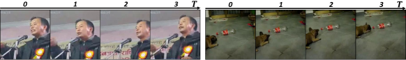
(a) Raw data

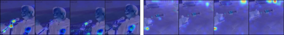
(b) Audiovisual attention (CLS-ER)

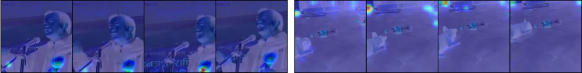
(c) Audiovisual attention (ESMER)

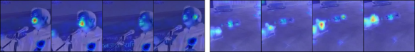
(d) Audiovisual attention (STELLA)

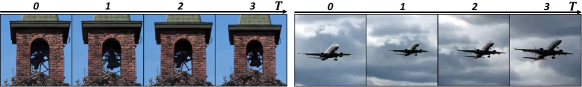
(a) Raw data

(b) Audiovisual attention (CLS-ER)

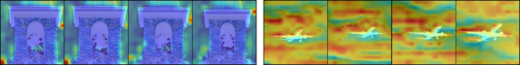
(c) Audiovisual attention (ESMER)

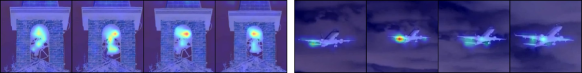
(d) Audiovisual attention (STELLA)

Figure 12: Sound source localization (a) Examples of raw video frames. (b)~(c): We visualize cross-attention maps using cosine similarity between each video patch and averaged audio embedding. (d): We use the AVM module in STELLA, continually pre-trained with the backbone mode, to visualize cross-attention maps. Our method is much more effective in capturing potential sound sources compared to the ability of the backbone to capture the sources.

Audiovisual event localization.

We conduct an audiovisual event localization (AVE) task to showcase the effectiveness of our method in precisely aligning audio and video streams. Following the experimental setup outlined in (Lin et al., 2023), we utilize the AVE dataset (Tian et al., 2018) for the experiment. To assess whether continually pre-trained models can adapt to the downstream task involving the unseen dataset, we use the model pre-trained on all tasks in the sequence within the Continual-VS experiment. The training process adheres to the hyperparameters described in Tab. 6, wherein the backbone model remains frozen while training the linear classifier. We present the summarized result in Tab. 8. This result demonstrates that our method surpasses other baseline methods. This underscores the strength of our method in adapting the downstream task that necessitates a sophisticated grasp of audio-video alignment at a high level.

Table 9: MSR-VTT audiovisual retrieval. MSR-VTT audiovisual retrieval task performances. We use the models continually pre-trained until completion of the last task of Continual-AS. The best and the second best results are highlighted in bold and underline, respectively.

Method	A$\rightarrow$V			V$\rightarrow$A
	R@1	R@5	R@10	R@1	R@5	R@10
Finetune	0.52	2.81	4.82	0.67	2.82	5.08
ER	1.48	6.70	11.48	1.74	7.19	12.07
MIR	1.56	5.97	10.23	1.85	6.93	11.89
DER++	2.74	9.08	14.49	2.45	9.49	14.60
GMED	2.07	8.04	13.11	2.70	8.44	12.89
CLS-ER	2.78	9.40	14.43	2.89	8.73	14.54
LUMP	2.33	8.15	12.75	2.04	7.93	12.45
ESMER	2.89	9.70	15.56	2.70	10.22	16.04
STELLA (Ours)	2.74	9.26	15.37	2.85	9.48	15.56
STELLA+ (Ours)	2.93	10.22	16.33	3.67	10.22	16.26

MSR-VTT retrieval task.

We provide additional experiment results on the MSR-VTT retrieval task in Tab. 9. In this experiment, we use the models continually pre-trained up to the last task of Continual-AS. We follow the training configurations in Tab. 6. The experiment results show that our methods consistently show competitive results, which supports that our methods obtain general audio-video correlations that are transferable to retrieval tasks.

Sound source localization.

We provide more visualization results of the sound source localization in Fig. 12. Our method consistently show superior ability in locating potential sound sources in the visual scenes.

Appendix F Hyperparamter Tuning Results

Patch sampling ratio.

Table 10: Retrieval result by sampling ratios.

Ratio(%) A$\rightarrow$V V$\rightarrow$A $\mathcal{A}\uparrow$ $\mathcal{F}\downarrow$ $\mathcal{A}\uparrow$ $\mathcal{F}\downarrow$ $\rho_{a}$ 37.5 13.76 4.77 13.52 5.53 50 14.16 4.38 14.07 4.65 62.5 13.77 5.04 13.46 5.06 $\rho_{v}$ 37.5 13.35 5.57 13.39 5.93 50 14.16 4.38 14.07 4.65 62.5 13.82 4.50 13.53 5.27

Central to our approach is the identification of patches that exhibit a high localized alignment with their corresponding modality pairs while being robust to catastrophic forgetting of learned representation, enabling the retention of meaningful information. Achieving the right balance in the sampling ratio is critical: an excessively low sampling ratio hinders the model from accessing essential data, while an overly high ratio hampers the model’s ability to disregard redundant or forget-inducing information.

For the audio sampling ratio, we systematically assess three options —37.5%, 50%, and 62.5%— while maintaining the video sampling ratio $\rho_{v}$ at 50%. Tab. 10 shows that sampling 50% of audio patches ensures high performance compared to the other sampling ratios. It is noteworthy that the other sampling ratios still yield competitive performance compared to the baselines. As we transition to optimizing the sampling ratio for video patches, we conduct experiments using three sampling ratios -37.5%, 50%, and 62.5%- alongside the audio sampling ratio $\rho_{a}$ at 50%. As demonstrated in Tab. 10, employing a 50% video sampling ratio ensures high performance.

Inference temperature in AVM module.

Table 11: Retrieval result by temperature values.

$\beta$ A$\rightarrow$V V$\rightarrow$A $\mathcal{A}\uparrow$ $\mathcal{F}\downarrow$ $\mathcal{A}\uparrow$ $\mathcal{F}\downarrow$ 0.1 13.91 5.42 14.23 4.97 0.4 14.16 4.38 14.07 4.65 0.5 13.37 5.27 13.50 5.84

In our approach, we actively harness cross-attention maps from the AVM module computed in Equation 1. During inference, we set the temperature hyperparameter $\beta$ to 0.4 for the Continual-VS experiments. To examine the significance of $\beta$, we explore a range of the hyperparameter values, specifically 0.1, 0.4, and 0.5. The results, as summarized in Tab. 11, indicate that the optimal temperature values typically reside within the range of approximately 0.1 to 0.4. This suggests the need for heightened emphasis on discriminative audio and video patches in order that those patches are more frequently selected in our selection framework in Equation 5 and in Algo. 2.

Appendix G Additional Analysis of Modality Gap

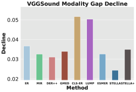
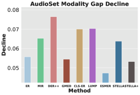
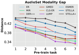
(a) Modality gap average decline		(b) Modality gap after each task

Figure 13: Modality gap estimation. (a): Average modality gap decline between the modality gap estimated at the completion of the last task and the modality gap estimated at the completion of each task. (b): Estimation of modality gap after the completion of each task (Continual-AS).

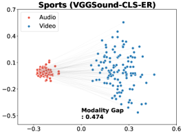
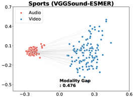
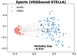
(a) Visualization in representation space (Continual-VS, sports)
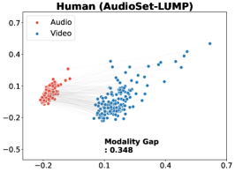
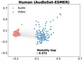
(b) Visualization in representation space (Continual-AS, human)

Figure 14: Modality gap visualization. (a): Visualizations of the modality gap corresponding to the sports task with the model pre-trained up to the last task in the Continual-VS experiment. (b): Visualization of the modality gap corresponding to the human task with the model pre-trained up to the last task in the Continual-AS experiment.

Comprehensive analysis

In the main paper, we examine the performance improvements of our approach in the context of continual audio-video pre-training with respect to the modality gap. In this section, we conduct a more detailed analysis; covering differences in the modality gap (Fig. 13 (a)), exploring the modality gap within the Continual-AS (Fig. 13 (b)), and providing additional visualizations of the modality gap to support the effectiveness of our approach (Fig. 13 (c)).

In Fig. 13 (a), our approach stands out with the smallest average modality gap difference. However, our approach does not exhibit high resistance to modality gap fluctuations within the Continual-AS experiment. An interesting observation emerges when comparing the average modality gap difference with the average forgetting in Tab. 1; a smaller average modality gap difference seems to correspond to lower average forgetting in the zero-shot retrieval tasks. This aligns with the relatively high average forgetting of our approach in the Continual-AS experiment, suggesting that the modality gap difference holds potential as a metric for assessing the extent of forgetting in audio-video correlation. Meanwhile, our approach consistently maintains the highest modality gap in all pre-train tasks (Fig. 13 (b)), which explains the high average accuracy of our approach in the Continual-AS retrieval tasks.

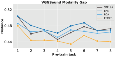
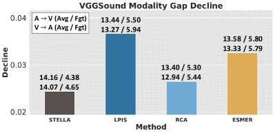
(a) Modality gap after each task	(b) Modality gap average decline

Figure 15: Modality gap estimation for each component of our proposed method. (a): Estimation of modality gap after completing each task. (b): Average decline in modality gap between the completion of the last task and the completion of each task.

We take our analysis a step further by visually representing the modality gap. In Fig. 14 (a), we visualize evaluation audio-video data pairs from the sports task in the Continual-VS experiments. Similarly, in Fig. 14 (b), we visualize data from the human task in the Continual-AS experiments. In both visualizations, we use the models that completed the continual pre-training phase. Remarkably, our approach consistently yields a larger gap in both cases. This suggests that the modality gap established from the initial task (sports, human) is effectively maintained, enabling the models to distinguish between different modalities, ultimately leading to enhanced performance.

Analysis on STELLA components

We estimate the modality gap of two key components within our proposed method: ELPP (Efficient Localized Patch Pooling Sec. 4.1) and RCA (Replay-guided Correlation Assessment Sec. 4.2). The ELPP consistently exhibits the highest modality gap across the tasks, as depicted in Fig. 15-(a). This underscores the effectiveness of the proposed method in Sec. 4.1 in identifying patches that demonstrate high localized alignment with their modality pairs. Consequently, the ELPP achieves better audio and video clustering within the multi-modal representation space, resulting in enhanced average accuracy in Tab. 4. This observation strongly supports our claim that the method outlined in Sec. 4.1 adeptly selects informative multi-modal patches from raw data.

The RCA illustrates a relatively minor modality gap difference, as indicated in Fig. 15-(b). During the continual pre-training, the modality gap between the audio and video exhibits robustness to the effect of changing distribution. Hence, the model maintains learned audio-video alignment. This explains the small average forgetting exhibited by the RCA in Tab. 4. It affirms our claim that the method introduced in Sec. 4.2 proficiently selects forget-robust patches.

Appendix H Audio Patch Selection Pseudo Code

Algorithm 2 Audio time chunk selection in a PyTorch-like Style.

  # I_a: audio patch importance score

  # P_a: audio pruning probability matrix

  # L_c: audio time chunk size

  # kappa_a: target number of audio tokens

  # num_time: the number of tokens in time dimension

  # num_freq: the number of tokens in frequency dimension

  def audio_time_chunk_selection(I_a,P_a):

        F_a=bernoulli(P_a)

        F_a=F_a.reshape(num_time, num_freq)

        F_a_t=F_a.sum(dim=1) # $\#$ of pruned patches

        I_a_t=I_a.reshape(num_time, num_freq)

        I_a_t=I_a_time.sum(dim=1) # Time-wise importance

        I_a_c=avg_pool(I_a_t, kernel_size=L_c) # Chunk-wise importance

        num_chunk=len(I_a_c)

        t_select=multinomial(I_a_c, num_samples=num_chunk)

        num_tokens=0

        for j in range(num_chunk):

             t=t_select[j]

             num_prune=F_a_t[t*L_c:(t+1)*L_c].sum() # $\#$ of pruned patches

             num_tokens+=(L_c*num_freq - num_prune) # Count $\#$ of patches

             if num_tokens > kappa_a:

                  F_last=F_a[t*L_c:(t+1)*L_c].view(-1)

                  F_last_accum=cumsum(flip($\sim$F_last))

                  prune_tail_idx= F_last_accum == num_tokens-kappa_a

                  F_last[-(prune_tail_idx+1):]=True # Prune tail of last chunk

                  F_a[t*L_c:(t+1)*L_c]=F_last.reshape(num_time,num_freq)

                  for k in range(j+1, num_chunk):

                      t_prune=t_select[k]

                      F_a[t_prune*L_c:(t_prune+1)*L_c]=True

                  break

        F_a=F_a.view(-1).float()

        S_tilde_a=argsort(F_a) # Forget-robust audio sorted indices

        return S_tilde_a

Appendix I Spatio-Temoporal Localized Alignment+ (STELLA+)

Algorithm 3 Continual Pre-training of STELLA+

0:  Dataset $\mathcal{D}_{i}$, model $f_{\theta,i-1}$, AVM module $h_{\Theta,i-1}$, rehearsal memory $\mathcal{M}$.

1:  for batch $(X_{a},\;X_{v})\sim\mathcal{D}_{i}$ do

2:     $\bm{k}_{a},\bm{q}_{a},\bm{A}_{a},\;\bm{k}_{v},\bm{q}_{v},\bm{A}_{v}\leftarrow\textsc{AVM}(X_{a},\;X_{v})$ COMMENT$\rhd$ Eq. 1

3:     $\bm{I}_{a},\;\bm{I}_{v}\leftarrow\textsc{Importance}(\bm{A}_{a},\;\bm{A}_{v})$ COMMENT$\rhd$ Eq. 2

4:     $\widehat{\bm{k}}_{a},\widehat{\bm{q}}_{a},\widehat{\bm{k}}_{v},\widehat{\bm{q}}_{v}\leftarrow\textsc{Sort}(\bm{k}_{a},\bm{q}_{a},\bm{I}_{a},\;\bm{k}_{v},\bm{q}_{v},\bm{I}_{v})$ COMMENT$\rhd$ Eq. 3

5:     $\widehat{X}_{a}^{p},\widehat{X}_{v}^{p},\;\widehat{\bm{q}}_{a}^{p},\widehat{\bm{q}}_{v}^{p}\leftarrow\mathcal{M}$

6:     $\bm{C}_{a},\;\bm{C}_{v}\leftarrow\textsc{Compare}(\widehat{\bm{k}}_{a},\widehat{\bm{q}}_{v},\widehat{\bm{q}}_{v}^{p},\;\widehat{\bm{k}}_{v},\widehat{\bm{q}}_{a},\widehat{\bm{q}}_{a}^{p})$ COMMENT$\rhd$ Eq. 4

7:     $\widehat{X}_{a}\leftarrow\textsc{Pick}(X_{a},\bm{I}_{a},\bm{C}_{a},)$

8:     $\widehat{X}_{v}\leftarrow\textsc{Pick}(X_{v},\bm{I}_{v},\bm{C}_{v})$ COMMENT$\rhd$ Eq. 6

9:     $\mathcal{M}\leftarrow\mathcal{M}\cup\left(\widehat{X}_{a},\widehat{X}_{v},\widehat{\bm{q}}_{a},\widehat{\bm{q}}_{v}\right)$

10:     $\Theta\leftarrow\Theta-\eta\nabla h_{\Theta,i-1}\left(X_{a},\;X_{v}\right)$

11:     $\theta\leftarrow\theta-\eta\nabla f_{\theta,i-1}\left([\widehat{X}_{a},\widehat{X}_{a}^{p}],\;[\widehat{X}_{v},\widehat{X}_{v}^{p}]\right)$

12:  end for

Appendix J Visualization of Fading Audio-Visual Attention

As shown in Fig. 2 of the main paper, we tackle the problem of forgetting past audio-video correlation by visualizing the attention maps. In Fig. 16, we provide additional examples that vividly illustrate the challenge of forgetting past correlation as the model undergoes pre-training on sequential tasks.

In the top-left example of Fig. 16, we observe a video example where a person is engaged in rope skipping. The initial attention map concentrated on the feet ((b)). However, as the model adapts to new tasks, the attention map is shifted solely to the person’s face ((c)), implying the gradual erosion of the correlation between the sound of rope skipping and the corresponding jumping motion. In the top-right example of Fig. 16, the attention map undergoes an intriguing shift towards an unrelated caption in the first two frames ((c)). Moving on to the middle-left example in Fig. 16, the model initially demonstrates a keen understanding of the xylophone’s location where the sound originates ((b)). However, subsequent training on additional tasks weakens auditory attention, and the model fails to locate the sounding region ((c)). This challenge becomes more pronounced when multiple sounding objects are involved. In the middle-right example in Fig. 16, we explore a scenario where a child is singing alongside a man playing the guitar. The initial visual attention map correctly identifies both the guitar and the child’s mouth. Nevertheless, as the model undergoes continuous training, the correlation between the singing voice and the child’s visual presence diminishes, and the model connects the sound with the guitar only ((c)). Similarly, in the bottom-left example of Fig. 16, the visual attention map shifts from the horse to the human, accompanied by the weakening of auditory attention towards the horse’s clip-clop sound ((b)). Lastly, in the bottom-right example of Fig. 16, despite the presence of only one prominent sounding object, the bird, the visual attention map is activated at the uncorrelated object. However, our approach successfully mitigates this forgetting problem, as demonstrated in (d) of the example, where the attention maps remain consistent with the initial attention maps.

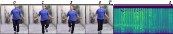
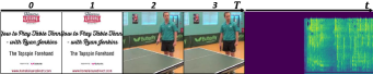
(a) Raw data

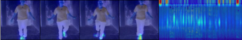
(b) Sparse audiovisual correlation

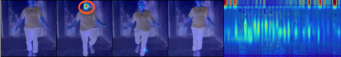
(c) Multimodal correlation forgetting (DER++)

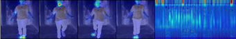
(d) Multimodal correlation forgetting (Ours)

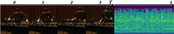
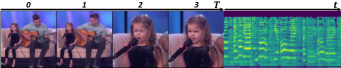
(a) Raw data

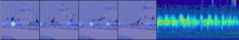
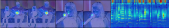
(b) Sparse audiovisual correlation

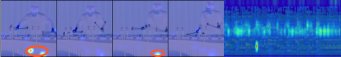
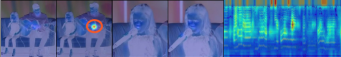
(c) Multimodal correlation forgetting (DER++)

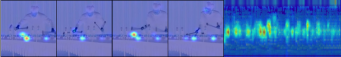
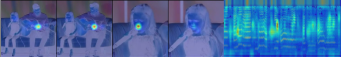
(d) Multimodal correlation forgetting (Ours)

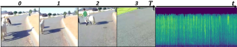
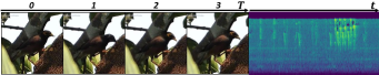
(a) Raw data

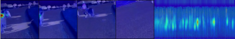
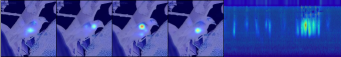
(b) Sparse audiovisual correlation

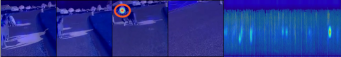
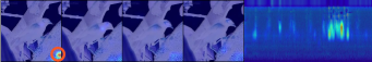
(c) Multimodal correlation forgetting (DER++)

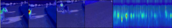
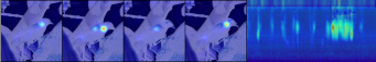
(d) Multimodal correlation forgetting (Ours)

Figure 16: Visualization of cross-attention maps. (a) Examples of raw data pairs. We visualize cross-attention maps of the pairs in (b). The closer the color is to red, the higher the attention score. While the baseline model using DER++ attends to entirely different parts as can be seen in (c), our method attends to a similar part even after being trained on two additional tasks as presented in (d). The wrong attention region is marked in an orange circle.

Appendix K Limiations

Our approach involves an extra inference step for patch selection, leveraging the AVM module on top of the backbone model. While this significantly reduces GPU memory consumption, it does incur additional computational overhead, yielding a relatively small improvement in throughput. To address this challenge, one potential solution is to develop a student model that integrates the AVM module and utilizes knowledge distillation to transfer audio-video representation from the backbone model. Recognizing the importance of enhancing efficiency, we acknowledge the necessity for future research to explore effective strategies for leveraging the AVM module. This avenue for improvement is a key component of our future research.

References

- Ahn et al. (2019) Ahn, H., Cha, S., Lee, D., and Moon, T. Uncertainty-based continual learning with adaptive regularization. In Advances in Neural Information Processing Systems (NeurIPS), 2019.
- Aljundi et al. (2019a) Aljundi, R., Caccia, L., Belilovsky, E., Caccia, M., Lin, M., Charlin, L., and Tuytelaars, T. Online continual learning with maximally interfered retrieval. CoRR, abs/1908.04742, 2019a.
- Aljundi et al. (2019b) Aljundi, R., Kelchtermans, K., and Tuytelaars, T. Task-free continual learning. In Proceedings of the IEEE International Conference on Computer Vision and Pattern Recognition (CVPR), 2019b.
- Arani et al. (2022) Arani, E., Sarfraz, F., and Zonooz, B. Learning fast, learning slow: A general continual learning method based on complementary learning system. In Proceedings of the International Conference on Learning Representations (ICLR), 2022.
- Buzzega et al. (2020) Buzzega, P., Boschini, M., Porrello, A., Abati, D., and Calderara, S. Dark experience for general continual learning: a strong, simple baseline. In Advances in Neural Information Processing Systems (NeurIPS), 2020.
- Chen et al. (2020) Chen, H., Xie, W., Vedaldi, A., and Zisserman, A. Vggsound: A large-scale audio-visual dataset. In IEEE International Conference on Acoustics, Speech and Signal Processing, 2020.
- Cossu et al. (2022) Cossu, A., Tuytelaars, T., Carta, A., Passaro, L. C., Lomonaco, V., and Bacciu, D. Continual pre-training mitigates forgetting in language and vision. CoRR, abs/2205.09357, 2022.
- Fini et al. (2022) Fini, E., da Costa, V. G. T., Alameda-Pineda, X., Ricci, E., Alahari, K., and Mairal, J. Self-supervised models are continual learners. In Proceedings of the IEEE International Conference on Computer Vision and Pattern Recognition (CVPR), 2022.
- Gemmeke et al. (2017) Gemmeke, J. F., Ellis, D. P. W., Freedman, D., Jansen, A., Lawrence, W., Moore, R. C., Plakal, M., and Ritter, M. Audio set: An ontology and human-labeled dataset for audio events. In IEEE International Conference on Acoustics, Speech and Signal Processing, ICASSP, 2017.
- Gong et al. (2023) Gong, Y., Rouditchenko, A., Liu, A. H., Harwath, D., Karlinsky, L., Kuehne, H., and Glass, J. R. Contrastive audio-visual masked autoencoder. In Proceedings of the International Conference on Learning Representations (ICLR), 2023.
- He et al. (2022) He, K., Chen, X., Xie, S., Li, Y., Dollár, P., and Girshick, R. B. Masked autoencoders are scalable vision learners. In Proceedings of the IEEE International Conference on Computer Vision and Pattern Recognition (CVPR), 2022.
- Hu et al. (2022a) Hu, X., Chen, Z., and Owens, A. Mix and localize: Localizing sound sources in mixtures. In Proceedings of the IEEE International Conference on Computer Vision and Pattern Recognition (CVPR), 2022a.
- Hu et al. (2022b) Hu, Y., Luo, C., and Chen, Z. Make it move: controllable image-to-video generation with text descriptions. In Proceedings of the IEEE International Conference on Computer Vision and Pattern Recognition (CVPR), 2022b.
- Huang et al. (2022a) Huang, P., Sharma, V., Xu, H., Ryali, C., Fan, H., Li, Y., Li, S., Ghosh, G., Malik, J., and Feichtenhofer, C. Mavil: Masked audio-video learners. CoRR, abs/2212.08071, 2022a.
- Huang et al. (2022b) Huang, P., Xu, H., Li, J., Baevski, A., Auli, M., Galuba, W., Metze, F., and Feichtenhofer, C. Masked autoencoders that listen. In Advances in Neural Information Processing Systems (NeurIPS), 2022b.
- Hwang et al. (2022) Hwang, S., Yoon, J., Lee, Y., and Hwang, S. J. Efficient video representation learning via masked video modeling with motion-centric token selection. CoRR, abs/2211.10636, 2022.
- Jin et al. (2021) Jin, X., Sadhu, A., Du, J., and Ren, X. Gradient-based editing of memory examples for online task-free continual learning. In Advances in Neural Information Processing Systems (NeurIPS), 2021.
- Kirkpatrick et al. (2016) Kirkpatrick, J., Pascanu, R., Rabinowitz, N. C., Veness, J., Desjardins, G., Rusu, A. A., Milan, K., Quan, J., Ramalho, T., Grabska-Barwinska, A., Hassabis, D., Clopath, C., Kumaran, D., and Hadsell, R. Overcoming catastrophic forgetting in neural networks. CoRR, abs/1612.00796, 2016.
- Korbar et al. (2018) Korbar, B., Tran, D., and Torresani, L. Cooperative learning of audio and video models from self-supervised synchronization. Advances in Neural Information Processing Systems (NeurIPS), 2018.
- Lee et al. (2023) Lee, J., Jang, S., Jo, J., Yoon, J., Kim, Y., Kim, J.-H., Ha, J.-W., and Hwang, S. J. Text-conditioned sampling framework for text-to-image generation with masked generative models. In Proceedings of the International Conference on Computer Vision (ICCV), 2023.
- Lee et al. (2020) Lee, S., Ha, J., Zhang, D., and Kim, G. A neural dirichlet process mixture model for task-free continual learning. In Proceedings of the International Conference on Learning Representations (ICLR), 2020.
- Lee et al. (2021) Lee, S., Yu, Y., Kim, G., Breuel, T. M., Kautz, J., and Song, Y. Parameter efficient multimodal transformers for video representation learning. In Proceedings of the International Conference on Learning Representations (ICLR), 2021.
- Li et al. (2020) Li, M., Zareian, A., Zeng, Q., Whitehead, S., Lu, D., Ji, H., and Chang, S.-F. Cross-media structured common space for multimedia event extraction. In Proceedings of the Association for Computational Linguistics (ACL), 2020.
- Liang et al. (2022) Liang, W., Zhang, Y., Kwon, Y., Yeung, S., and Zou, J. Y. Mind the gap: Understanding the modality gap in multi-modal contrastive representation learning. In Advances in Neural Information Processing Systems (NeurIPS), 2022.
- Liao et al. (2022) Liao, W., Hu, K., Yang, M. Y., and Rosenhahn, B. Text to image generation with semantic-spatial aware gan. In Proceedings of the IEEE International Conference on Computer Vision and Pattern Recognition (CVPR), 2022.
- Lin et al. (2023) Lin, Y.-B., Sung, Y.-L., Lei, J., Bansal, M., and Bertasius, G. Vision transformers are parameter-efficient audio-visual learners. In Proceedings of the IEEE International Conference on Computer Vision and Pattern Recognition (CVPR), 2023.
- Liu et al. (2023) Liu, H., Li, C., Wu, Q., and Lee, Y. J. Visual instruction tuning. arXiv preprint arXiv:2304.08485, 2023.
- Liu et al. (2022) Liu, X., Qian, R., Zhou, H., Hu, D., Lin, W., Liu, Z., Zhou, B., and Zhou, X. Visual sound localization in the wild by cross-modal interference erasing. In Proceedings of the AAAI National Conference on Artificial Intelligence (AAAI), 2022.
- Madaan et al. (2022) Madaan, D., Yoon, J., Li, Y., Liu, Y., and Hwang, S. J. Representational continuity for unsupervised continual learning. In Proceedings of the International Conference on Learning Representations (ICLR), 2022.
- Mo et al. (2023) Mo, S., Pian, W., and Tian, Y. Class-incremental grouping network for continual audio-visual learning. CoRR, abs/2309.05281, 2023.
- Nagrani et al. (2021) Nagrani, A., Yang, S., Arnab, A., Jansen, A., Schmid, C., and Sun, C. Attention bottlenecks for multimodal fusion. In Advances in Neural Information Processing Systems (NeurIPS), 2021.
- Pian et al. (2023) Pian, W., Mo, S., Guo, Y., and Tian, Y. Audio-visual class-incremental learning. CoRR, abs/2308.11073, 2023.
- Rebuffi et al. (2017) Rebuffi, S., Kolesnikov, A., Sperl, G., and Lampert, C. H. icarl: Incremental classifier and representation learning. In Proceedings of the IEEE International Conference on Computer Vision and Pattern Recognition (CVPR), 2017.
- Rolnick et al. (2019) Rolnick, D., Ahuja, A., Schwarz, J., Lillicrap, T. P., and Wayne, G. Experience replay for continual learning. In Advances in Neural Information Processing Systems (NeurIPS), 2019.
- Sarfraz et al. (2023) Sarfraz, F., Arani, E., and Zonooz, B. Error sensitivity modulation based experience replay: Mitigating abrupt representation drift in continual learning. In Proceedings of the International Conference on Learning Representations (ICLR), 2023.
- Tang et al. (2022) Tang, Z., Cho, J., Nie, Y., and Bansal, M. TVLT: textless vision-language transformer. In Advances in Neural Information Processing Systems (NeurIPS), 2022.
- Tian et al. (2018) Tian, Y., Shi, J., Li, B., Duan, Z., and Xu, C. Audio-visual event localization in unconstrained videos. In Proceedings of the European Conference on Computer Vision (ECCV), 2018.
- Tian et al. (2020) Tian, Y., Li, D., and Xu, C. Unified multisensory perception: Weakly-supervised audio-visual video parsing. In Proceedings of the European Conference on Computer Vision (ECCV), 2020.
- Udandarao (2022) Udandarao, V. Understanding and Fixing the Modality Gap in Vision-Language Models. PhD thesis, 2022.
- Villegas et al. (2022) Villegas, R., Babaeizadeh, M., Kindermans, P.-J., Moraldo, H., Zhang, H., Saffar, M. T., Castro, S., Kunze, J., and Erhan, D. Phenaki: Variable length video generation from open domain textual description. arXiv preprint arXiv:2210.02399, 2022.
- Vitter (1985) Vitter, J. S. Random sampling with a reservoir. ACM Trans. Math. Softw., 1985.
- Xiao et al. (2020) Xiao, F., Lee, Y. J., Grauman, K., Malik, J., and Feichtenhofer, C. Audiovisual slowfast networks for video recognition. arXiv preprint arXiv:2001.08740, 2020.
- Xu et al. (2016) Xu, J., Mei, T., Yao, T., and Rui, Y. MSR-VTT: A large video description dataset for bridging video and language. In Proceedings of the IEEE International Conference on Computer Vision and Pattern Recognition (CVPR), 2016.
- Yan et al. (2023) Yan, R., Shou, M. Z., Ge, Y., Wang, J., Lin, X., Cai, G., and Tang, J. Video-text pre-training with learned regions for retrieval. In Proceedings of the AAAI National Conference on Artificial Intelligence (AAAI), 2023.
- Yan et al. (2022) Yan, S., Hong, L., Xu, H., Han, J., Tuytelaars, T., Li, Z., and He, X. Generative negative text replay for continual vision-language pretraining. In Proceedings of the European Conference on Computer Vision (ECCV), 2022.
- Yoon et al. (2018) Yoon, J., Yang, E., Lee, J., and Hwang, S. J. Lifelong learning with dynamically expandable networks. In Proceedings of the International Conference on Learning Representations (ICLR), 2018.
- Yoon et al. (2023) Yoon, J., Hwang, S. J., and Cao, Y. Continual learners are incremental model generalizers. In Proceedings of the International Conference on Machine Learning (ICML), 2023.
- Zenke et al. (2017) Zenke, F., Poole, B., and Ganguli, S. Continual learning through synaptic intelligence. In Proceedings of the International Conference on Machine Learning (ICML), 2017.
- Zhou et al. (2019) Zhou, H., Liu, Y., Liu, Z., Luo, P., and Wang, X. Talking face generation by adversarially disentangled audio-visual representation. In Proceedings of the AAAI National Conference on Artificial Intelligence (AAAI), 2019.