Geometry of the magnetic Steklov problem on Riemannian annuli
Abstract. We study the geometry of the first two eigenvalues of a magnetic Steklov problem on an annulus (a compact Riemannian surface with genus zero and two boundary components), the magnetic potential being the harmonic one-form having flux around any of the two boundary components. The resulting spectrum can be seen as a perturbation of the classical, non-magnetic Steklov spectrum, obtained when and studied e.g., by Fraser and Schoen in [8, 9]. We obtain sharp upper bounds for the first and the second normalized eigenvalues and we discuss the geometry of the maximisers.
Concerning the first eigenvalue, we isolate a noteworthy class of maximisers which we call -surfaces: they are free-boundary surfaces which are stationary for a weighted area functional (depending on the flux) and have proportional principal curvatures at each point; in particular, they belong to the class of linear Weingarten surfaces.
Inspired by [8], we then study the second normalized eigenvalue for a fixed flux and prove the existence of a maximiser for rotationally invariant metrics. Moreover, the corresponding eigenfunctions define a free-boundary immersion in the unit ball of . Finally, we prove that the second normalized eigenvalue associated to a flux has an absolute maximum when , the corresponding maximiser being the critical catenoid.
Keywords: Magnetic Laplacian, Steklov problem, first and second eigenvalue, maximisation, conformal modulus, free-boundary immersions, -surfaces.
2020 Mathematics Subject Classification: 58J50, 58J32, 35P15, 53C42
1 Introduction
This paper deals with a magnetic Steklov problem on a Riemannian annulus with smooth boundary . For the precise definitions we refer to Subsection 1.1 below. We are interested in sharp inequalities for the first two eigenvalues, and in the geometry of the optimizers. First, we review the main features of the classical (non-magnetic) Steklov problem on Riemannian surfaces. Then we give a short summary of the type of results that we obtain in the magnetic case.
1.1 The non-magnetic case
Let be a connected Riemannian surface with boundary . The classical Steklov problem (see [18]) is:
| (1) |
Here is the exterior unit normal to and is the Laplace-Beltrami operator. It is well-known that (1) admits a discrete sequence of non-negative eigenvalues of finite multiplicity, diverging to :
The first eigenvalue is zero, with associated eigenfunctions given by the constants. In this paper the first positive eigenvalue of (1) will be numbered : the reason is that in the magnetic case we will consider the first eigenvalue which, very often, is positive.
An isoperimetric inequality for was given by Weinstock (see [19]). To recall it, first observe that the -th normalized eigenvalue, distinguished by a bar:
is invariant by homotheties.
Theorem 1 (Weinstock, 1954).
If is a simply connected planar domain, then Equality holds if and only if is a disk.
The upper bound is valid, more generally, for any simply connected Riemannian surface. For an arbitrary topology the following upper bound was proved in [10]:
Theorem 2 (Girouard-Polterovich, 2012).
If is a Riemannian surface with genus and boundary components we have:
| (2) |
The previous bound can be refined in the case of annuli: by definition, a Riemannian annulus (or simply, an annulus) is a Riemannian surface having genus zero and two boundary components. It is a Riemannian surface diffeomorphic to the flat annulus . In this case, (2) reads , which is not sharp because one has the following result proved in [8]:
Theorem 3 (Fraser-Schoen, 2011).
Let be the positive root of the equation . Then, for any rotationally invariant annulus one has:
Equality holds for a particular rotation surface , called critical catenoid.
Note that . After some deep additional work, the authors were able to extend the result to all annuli in [9]:
Theorem 4 (Fraser-Schoen, 2016).
For any annulus one has . Hence the critical catenoid is an absolute maximum for the lowest (positive) normalized Steklov eigenvalue on annuli.
The critical catenoid has remarkable geometric properties: it is the unique rotational annulus which is minimal and free boundary in the unit ball of , where free boundary means that and meets the boundary of orthogonally. To construct , consider the rotational surface in obtained by rotating the curve (profile) around the -axis. Draw the line from the origin which is tangent to the profile: the slice that we obtain is free boundary in a certain ball of radius . Scaling back to we obtain the critical catenoid.
Minimal free boundary immersions are stationary points of the area functional for variations of keeping its boundary on . The theory of minimal free boundary immersions is in some ways reminiscent of the theory of minimal spherical immersions, although it is very different in many respects. There are many well established results relating the maximisers for the -th normalized eigenvalue of closed Riemannian surfaces to minimal immersions in for some (see e.g., [5, 6, 14, 16]). Fraser and Schoen [9] showed that, when dealing with Riemannian surfaces with boundary, maximisers for the -th normalized eigenvalue of the Steklov problem give rise to minimal free boundary immersions in some Euclidean unit ball.
1.2 Perturbation of the Laplacian by a magnetic flux
In this paper we consider a Steklov spectrum by introducing the magnetic Laplacian associated to a closed potential one-form of flux on any annulus , the flux being the circulation of around any of the two boundary curves of (the two circulations are the same because is closed). This leads to the perturbed spectrum
which in fact depends only on the flux (by the gauge invariance property of the magnetic Laplacian) and which we will call magnetic Steklov spectrum of flux . We denote it by . It has the property of being periodic: for all integers , and remains unchanged when is replaced by . Hence, it is enough to study the spectrum when the flux takes value in the interval ; in particular, if the flux is an integer, the spectrum reduces to the classical, non-magnetic Steklov spectrum .
We will postpone the precise definition and the properties of the magnetic Laplacian and its Steklov spectrum to Section 2.
From now on, we assume .
The magnetic Steklov spectrum is a perturbation of the usual Steklov spectrum in the sense that as (more generally, as tends to an integer).
We now briefly describe the results that we obtain for and . As in the classical case, we are interested in the normalized eigenvalues , which turn out to be invariant by homotheties for all fixed .
Upper bound of the first eigenvalue. We first recall that in the non-magnetic case the first eigenvalue is always zero, with associated eigenspace being given by the constant functions; actually, we have that if and only if is an integer. Therefore, the geometric invariants arising in the study of , which is positive when is not an integer, are peculiar to the magnetic situation, and do not have, at least a priori, a non-magnetic counterpart. Analogies with the classical case can be looked for when one examines the second eigenvalue which, when , reduces to the first positive non-magnetic Steklov eigenvalue.
Having said that we first give a sharp, conformal upper bound of for all annuli . The result reads:
where is the so-called conformal modulus of (see Subsection 2.2 for the definition). When is an arbitrary real number, the upper bound holds with replacing on the right hand side. This is presented in Theorem 16.
Again, in the non-magnetic case both sides are zero, and there is nothing to say.
The upper bound turns out to be exact asymptotically as , in the sense that, for any annulus , one has that as : loosely speaking, this means that one can “hear” the conformal class of knowing the lowest normalized eigenvalue for all sufficiently small. This result is presented in Theorem 17.
Upper bound of the second eigenvalue. Then, in Theorem 22 we give a sharp upper bound of the second normalized eigenvalue for any value of the flux and for all rotationally invariant annuli. It is enough to state it when :
| (3) |
When , the constant denotes the unique positive root of the equation (it tends to when ). In particular we show that, if the flux is not a half-integer, a maximiser for exists in the class of all rotationally invariant annuli. Of course, the result when is due to Fraser and Schoen [8]. The upper bound in (3) is continuous and decreasing in for (see Corollary 23), hence we get:
which implies the following fact.
Theorem 5.
The critical catenoid maximizes among all rotationally invariant annuli, for all values of the flux .
This generalises [8] (i.e., ) to the magnetic case. We conjecture that the theorem holds for all annuli, and not just in the rotationally invariant case.
Geometry of maximisers. We then study the geometry of maximisers and ask the following question:
are the maximisers (conformally) minimal in some sense and free boundary in the unit ball of ?
For the first eigenvalue , we show that the maximisers are conformally equivalent to free boundary rotation surfaces which are minimal for the weighted area
for some value depending on the conformal modulus of , where is the distance to the axis of rotation (see Theorem 31). We then have a family of distinguished free boundary surfaces, which we call critical -surfaces: they foliate the unit ball in and have interesting geometric properties, for example their principal curvatures are proportional at every point ( where is the meridian curvature). In particular, these maximisers are a particular case of surfaces already known to differential geometers, called Weingarten surfaces. The critical catenoid is the member of the family corresponding to . We give a list of equivalent characterizations of -surfaces (one of them involving the magnetic Laplacian) in Theorem 27.
Concerning the maximisers of , we observe that the multiplicity of the corresponding eigenvalue is , and the (suitably normalized) eigenfunctions define a free boundary immersion in the unit ball which is minimal in an appropriate sense, see Theorems 34 and 36. We plan to investigate the variational meaning of this notion of minimality in a forthcoming paper.
In this paper we have considered the case of Riemannian annuli, that is, Riemannian surfaces of genus and boundary components. The easiest setting for studying maximisers for magnetic Steklov eigenvalues and their geometry is the simply connected case. In this case, the analogous inequality of Weinstock for has been proved in [3]: namely, among all simply connected Riemannian surfaces, the first normalized eigenvalue is maximised (up to -homotheties) by a planar disk centered at the pole of the magnetic potential , and the maximum value is .
The present paper is organized as follows. In Section 2 we introduce the magnetic Laplacian on Riemannian surfaces, in particular on Riemannian annuli, and we list some relevant properties and definitions. In Section 3 we compute explicitly the spectrum of rotationally invariant, symmetric annuli and identify the first and second eigenvalue. In Section 4 we state the results on the maximisation of the first normalized eigenvalue, while in Section 5 we state the results on the maximisation of the second normalized eigenvalue. In Section 6 we discuss the geometry of maximisers of while in Section 7 we discuss the geometry of maximisers of . All the proofs are contained in a series of appendices. Namely, the proofs of the results of Sections 2, 4, 5, 6, 7 are contained, respectively, in Appendices A, B, C, D, E.
2 The magnetic Laplacian on Riemannian annuli
2.1 The magnetic Laplacian
Let be a Riemannian surface, with or without boundary, and let be a smooth real one-form on . The two-form is called the magnetic field and is the potential one-form. The magnetic Laplacian associated with the pair is denoted by and acts on smooth complex valued functions as follows:
where is the magnetic differential and for all one-forms , where is the dual vector field of . is also called the magnetic co-differential. More explicitly:
The magnetic Steklov problem amounts to finding all -harmonic functions and all eigenvalues satisfying the problem:
| (4) |
where is the outer unit normal to . It is well-known that the spectrum is non-negative, discrete, and increasing to ; we stress that it depends on the pair and, of course, not only on :
From a variational point of view, the magnetic Laplacian is naturally associated to the energy quadratic form
and hence we have the usual min-max characterization of the eigenvalues:
| (5) |
where is the usual Sobolev space of functions in with first order derivatives in . Of course, the Steklov problem when reduces to the classical (non-magnetic) Steklov problem. Actually, this happens in greater generality. In fact, gauge invariance implies that the spectrum of is the same as the spectrum of for any real function on , which follows from the fact that and are unitarily equivalent. Thus, in treating the eigenvalues, we have the freedom to alter the potential one-form by any exact one-form.
A bit more generally, we have gauge invariance also when is closed and the flux of around any closed curve in is an integer: by definition, if is a loop (a continuous curve such that ) the number
is called the flux of along . We remark that the orientation of the loop does not affect the spectrum, hence we do not need to specify it. Summarizing, we have the following fact:
Proposition 6.
In the above notation, we have if and only if is closed and the flux of around any closed curve is an integer.
In this paper we shall investigate the case when the magnetic field is zero, i.e., when the potential one-form is closed.
2.2 The magnetic Laplacian with zero magnetic field on an annulus
The purpose of this paper is to investigate the magnetic Steklov problem when the one-form is closed and is an annulus, that is, a Riemannian surface diffeomorphic to
Then, has genus zero and two boundary components. The absolute de Rham real cohomology in degree one of an annulus is one-dimensional. Cohomology classes are indexed by the flux of closed one-forms around any of the two boundary components : in fact, these two fluxes are the same because is closed, by the Stokes theorem. Let be any two closed one-forms with fluxes which differ by an integer; if one considers the magnetic Laplacians associated to the pairs and , we see they are unitarily equivalent by the Shigekawa argument discussed in the previous subsection (see [17], see also [3]), and therefore have the same Steklov spectrum. Then, writing
we will denote the -th eigenvalue of the Steklov problem associated with any closed potential of flux , without ambiguity. In particular, note that, if is not an integer, then
while in the classical Steklov case () we have of course with associated eigenspace given by the constant functions. We will keep this notation, so that, according to this numbering, the writing will denote the first positive eigenvalue of the usual non-magnetic Steklov problem.
Note that since is closed the magnetic field is zero; however, as we have said, if , the ground state energy is positive: this phenomenon is vaguely referred, in the physics literature, as the Aharonov-Bohm effect (for a discussion of this physical phenomenon, we refer to [1]). We can always assume, by gauge invariance, that ; but in fact, since replacing by the spectrum remains invariant (and the eigenfunctions change to their conjugates), we can assume
Definition 7 (Conformal modulus).
Any annulus is conformally equivalent to the cylinder
for a unique , which is called the conformal modulus of . In other words, any annulus is isometric to endowed with the metric for a smooth .
If the metric of is rotationally invariant (i.e., it does not depend on ), then so does the conformal factor . In particular, to any surface of revolution in can be associated a metric of type: on some .
2.3 Conformal invariance of magnetic Dirichlet energy
We recall here a fundamental property of the magnetic Dirichlet energy, analogous to the conformal invariance of the usual Dirichlet energy in two dimensions. Let be a magnetic pair (surface and real one-form) and let be a conformal map of Riemannian surfaces. Then for all one has:
where is as usual the potential one-form on given by pull-back of and . For a proof of this result we refer to [3].
2.4 Normalized eigenvalues and -homotheties
Let be the magnetic Steklov spectrum of a Riemannian annulus with flux . The -th normalized eigenvalue is by definition . It is easy to see that it is invariant by homotheties, exactly as in the non-magnetic case, but even more is true.
Definition 8 (-homothety).
Given two surfaces with boundary , a -homothety between them is a conformal diffeomorphism which restricts to a homothety on . Equivalently, the map
( and being the respective metrics) is a -homothety if and only if for a smooth function on , and the conformal factor is constant on the boundary of .
The following result is well-known in the non-magnetic case, but extends also to any flux .
Proposition 9.
If two annuli are -homothetic, then they have the same normalized spectrum for all fluxes :
for all .
The proof is presented in Appendix A.
2.5 Rotationally invariant annuli
Let be a rotationally invariant annulus with conformal modulus : then, it is isometric with endowed with the metric where now . In addition, we say that is symmetric if (this is true, in particular, if is an even function: ). This implies that the two boundary components have the same length, which guarantees that is -homothetic with the cylinder . We remark that any surface in obtained by rotating around the -axis the graph of on , with even, is a symmetric annulus.
From Proposition 9 we deduce the following:
Proposition 10.
Any rotationally invariant, symmetric annulus of conformal modulus has the same normalized spectrum of the cylinder .
3 Normalized spectrum of rotationally invariant, symmetric annuli
In this section we compute explicitly the magnetic Steklov spectrum with zero magnetic field of rotationally invariant, symmetric annuli for closed potential one-forms.
3.1 Flat annuli
A flat annulus is the product with coordinates , endowed with the flat metric . We take as magnetic potential the harmonic one-form which has flux around . We can think of as a cylinder in , and in this case the one-form can be expressed in Cartesian coordinates as (and is defined on the whole ). Since is harmonic (hence co-closed) the magnetic Laplacian is given by:
We now look for solutions of ; as customary we separate variables, and consider functions of the form , . Since the metric is flat we have
Moreover, and , so that
It follows that
So, if we want , we must solve the ODE on the interval . The general solution is
when . If is an integer and we have , . Since the case is exactly the classical Steklov problem, for which the spectrum on cylinders has been extensively described (see e.g., [11]), we shall assume from now on (unless explicitly stated) that . In the following subsection we consider separately the linearly independent solutions (solutions of first type) and (solutions of second type).
Solutions of the first type. The first type of solution is . Note that on and on , so that we easily compute
Hence is a Steklov eigenfunction associated to
Solutions of the second type. We now take . Then:
and is a Steklov eigenfunction associated to
A standard argument allows to prove that these solutions are all the magnetic Steklov eigenfunctions on (see [3] for a proof of this fact in the case of a disk, see also [11]). We have the following:
Theorem 11.
The Steklov spectrum of the magnetic Laplacian on the flat cylinder when is given by the collection of all where
When (or, more in general, when ) we know that the spectrum is given by
3.2 Normalized spectrum of rotationally invariant, symmetric annuli
Throughout this section, we denote by any rotationally invariant symmetric annulus having conformal modulus (an example is the flat annulus discussed in the previous subsection).
Since the boundary of consists of two circles of radius one, and since any rotationally invariant symmetric annulus of conformal modulus has the normalized spectrum of (see Proposition 10), we have the following description of the normalized spectrum: note that it depends only on and .
Theorem 12.
Let be a rotationally invariant, symmetric annulus of conformal modulus . Then its normalized spectrum is given by the collection of all where:
If , we have , .
We now discuss the magnetic case: hence we can restrict to the interval . We identify the first and the second eigenvalue as follows.
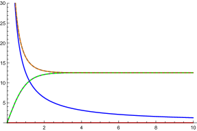
Proposition 13 (First eigenvalue).
Assume . The first normalized eigenvalue of a rotationally invariant, symmetric annulus of conformal modulus is
Again note that when , , with corresponding constant eigenfunctions. When the associated eigenfunction is , which is real and radial, in the sense that it does not depend on the angular variable ; then (see the proof of Proposition 10) the same happens for any rotationally invariant, symmetric annulus .
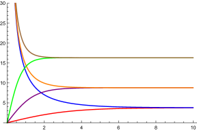
Now we turn to the second eigenvalue. There are two competing branches:
| (6) |
so that we have:
Proposition 14 (Second eigenvalue).
a) Fix . The second normalized eigenvalue of a rotationally invariant, symmetric annulus of conformal modulus is
b) If then:
In that case has multiplicity for all values of the conformal modulus .
We now fix and discuss the supremum of as a function of the conformal modulus , that is, we set:
and, for , we let be the unique positive root of the equation .
Proposition 15.
Let be a rotationally invariant, symmetric annulus of conformal modulus .
(a) Fix . Then is attained for the unique value ; that is
For this value the second eigenvalue has multiplicity , and we have .
(b) Fix . Then is not attained for any finite value of . In fact , and is reached asymptotically as . Moreover, for any finite value of one has .
For the proof of (a), just observe that, as increases, the first branch in (6) increases from to , while the second decreases from to : since , the two branches meet precisely when , which realizes the maximum.
When we see immediately that for all ; the sup is attained only when and takes the value .
Finally, one can easily check that when the two competing branches are and , and in this case is the unique positive root of .

4 Sharp upper bound for the first normalized eigenvalue
In this section we consider inequalities for the first normalized eigenvalue. The first result is a sharp upper bound valid for any annulus (not necessarily rotationally invariant).
Theorem 16.
Let be a Riemannian annulus. Then, for all :
| (7) |
where is the conformal modulus of . If , equality holds if and only if is -homothetic to the cylinder . In particular, the following uniform upper bound holds:
independently of the conformal modulus.
We have seen that the estimate becomes an equality for all rotationally invariant, symmetric annuli. If we don’t fix the conformal modulus, then the upper bound is never attained, and it is reached asymptotically by families of rotationally invariant, symmetric annuli of conformal modulus .
We remark once again that if is arbitrary the upper bound holds with replacing in the right hand side.
The proof is presented in Appendix B.
In the rest of this subsection we discuss some remarks on the sharpness of the estimate of Theorem 16.
4.1 Asymptotics of the first normalized eigenvalue as
A first remark is that in fact every Riemannian annulus realizes equality in (7) asymptotically as , in the following sense:
Theorem 17.
For any Riemannian annulus (not necessarily rotationally invariant) one has:
That is, asymptotically as :
For the proof we refer to Appendix B. This inequality says that the magnetic Steklov spectrum detects the conformal modulus of an annulus, in the sense that if we know for a sequence of fluxes , then we also know the conformal modulus of .
4.2 The case of planar annuli
Another remark concerns the inequality of Theorem 16 for all : in this subsection, we examine the possibility of improving it when is a planar annulus.
Let be the concentric annulus in the plane bounded by the concentric circles of radii and : centered at the origin. In this case we can take, as magnetic potential, the one-form , where is the angular variable in polar coordinates in : in fact, is closed and has flux around both circles bounding . Simple explicit calculations (which we omit for brevity) show that
where is any disk centered at . Moreover as . This simple observation might suggest the following conjecture:
is it true that every doubly connected planar domain has first normalized Steklov eigenvalue smaller than ?
A bit surprisingly, one has the following result:
Theorem 18.
There exists a sequence of doubly connected planar domains such that, for any fixed :
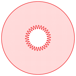
For the proof we refer to Appendix B. In other words, there exist sequences of planar annuli which saturate the inequality . As a consequence of Theorem 16, it follows that the conformal modulus of the annuli in these families tends to as . From the proof it can be easily deduced that the ratio of the two boundary lengths of tends to as . Again, this is not a surprise in view of Theorem 16. A prototypical example of a domain is illustrated in Figure 2.
5 Upper bound for the second normalized eigenvalue for rotationally invariant annuli
Through all this section we assume . As we have already mentioned, the case is the classical case of the Laplacian and has been treated in [8]. For we have seen in Section 3 that the first eigenvalue of a rotationally invariant, symmetric annulus is always double, and it has no maximum if we do not restrict to a fixed conformal class of annuli.
Recall that we have defined
where denotes a rotationally invariant symmetric annulus of conformal modulus : every such domain is in fact isospectral (for the normalized spectrum) to the flat annulus . Hence we can write
We have seen in Proposition 15 that
where is the unique root of the equation . We summarize these facts in the following theorem:
Theorem 19.
Let be a rotationally symmetric, invariant annulus. Then, for all , one has:
Equality holds if and only if has conformal modulus .
We prove in Appendix C the two following fundamental lemmas which describe the behavior of and as functions of .
Lemma 20.
The function is increasing, and moreover:
where is the unique positive root of the equation . That is, maps one-to-one to .
Note that is the conformal modulus of the critical catenoid.
Lemma 21.
The function is decreasing, and we have:
where is the conformal modulus of the critical catenoid. Therefore for all (hence, also for all ) one has
where is the second normalized non-magnetic Steklov eigenvalue (i.e., for ) of the critical catenoid.
We are able to prove that Theorem 19 holds without the symmetry assumption, namely, it holds for all rotationally invariant annuli. This is the main result of this section.
Theorem 22.
Let be a rotationally invariant annulus. Then
where and is the unique positive root of . Equality holds if and only if is -homothetic to .
This result is the analogue of [8] for the non-magnetic Steklov case. We prove this theorem in Section C. As a corollary we have
Corollary 23.
For any rotationally invariant annulus and any flux one has the upper bound:
with equality if and only if is an integer and is -homothetic to the critical catenoid.
Hence equality holds if and only if ia an integer and admits a free boundary conformal minimal immersion in the unit ball which restricts to a homothety on the boundary.
We believe that the upper bound of Theorem 22 holds for any annulus.
Concerning the case of , we recall from Section 3 that for rotationally symmetric, invariant annuli, the first eigenvalue is double: . Hence there is no maximiser for in the class of rotationally invariant, symmetric annuli, , and is reached asymptotically by families of rotationally invariant, symmetric annuli with . In view of Theorem 22, the same considerations hold if we consider rotationally invariant annuli.
6 Geometry of maximisers: first eigenvalue
Theorem 16 says that among all annuli of conformal modulus , has a maximum: . A maximiser is the cylinder , and any annulus -homothetic to . In this section we consider some distinguished representatives of the maximiser in the conformal class and study their geometric properties. Inspired by the work of Fraser and Schoen [8] we ask the following question: is there a noteworthy class of free boundary rotation surfaces which realize the equality? Are these surfaces minimal in some sense?
We will think of as being obtained by rotating the graph of the function around the -axis over an interval and we assume for all . Hence a parametrization can be:
Note that the function measures the distance to the axis of rotation (the -axis). Through all the paper, we use to denote the radial coordinate in for the cylindrical coordinates . In Cartesian coordinates , .
Definition 24 (-surface).
Let be a real parameter. We say that the rotation surface is an -surface if the profile satisfies
| (8) |
These surfaces are examples of the so-called Weingarten surfaces, that is, surfaces whose principal curvatures and satisfy a certain functional relation . In fact, it turns out that the principal curvatures of -surfaces are proportional (see Theorem 27 here below). These surfaces have been considered in [4]. More recently, the complete classification of rotation surfaces in whose principal curvatures satisfy a linear relation has been obtained in [15].
Up to homotheties in , there is a unique -surface. As a reference -surface we take the one whose profile solves the problem:
Here can be also . This surface is symmetric about the -plane.
Example 25.
For the solution is hence -surfaces are simply the catenoids.
Example 26.
For the solution is , which means that -surfaces are round spheres.
In the next theorem we review the geometric properties of the -surfaces: in particular, note the characterization which asserts that the -surface is minimal in a weighted sense.
Theorem 27.
Let be a rotation surface. The following are equivalent:
-
a)
is an -surface.
-
b)
The principal curvatures are proportional; precisely, if denotes the meridian curvature (which coincides with the curvature of the profile), then one has at every point
-
c)
is critical for the functional .
-
d)
The function is a -harmonic function on , where is the harmonic one-form having flux around any parallel circle.
The equivalence between a) and b) was proved in [4]. The equivalence between a), c) and d) appears to be new. In particular, the equivalence between a) and c) extends Euler’s theorem (stating that the only minimal rotation surface is a catenoidal slab) to rotation surfaces which are stationary for the weighted area (Euler’s theorem being the case ).
The equivalence between a) and d) has further spectral consequences, see Section 6.2 below.
We prove the theorem in Appendix D. We note that the function is -harmonic in , where denotes the magnetic Laplacian in and is the potential one-form in given by : in fact, this specific restricts to on .
Observe also that when the weighted area in c) is the usual area, and in fact -surfaces (i.e. catenoids) are minimal in the classical sense.
6.1 Critical -surface and the first eigenvalue
We now restrict to the case , so that the profile of the corresponding -surface is convex. We conduct the line from the origin in the -plane () which is tangent to the profile: the contact point is unique and finite by the convexity of the profile and by the fact that decreases from to (see e.g., [4], see also the proof of Lemma 40). Therefore the surface obtained by rotation of the graph above the interval is free boundary in the ball of radius .
Definition 28 (Critical -surface).
Let be as above, and let be the surface obtained by rotating the graph above the interval . Scaling to the unit ball, we get a unique free boundary -surface. We call it the critical -surface.
Example 29.
The critical -surface is just the critical catenoid .
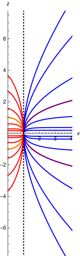
It is not difficult to see that the family of critical -surfaces for foliate the unit -ball minus the segment joining the two poles, and as degenerates to , see Figure 4.
Let be the conformal modulus of the critical -surface. We have the following monotonicity property of :
Proposition 30.
The function is decreasing from to , that is:
The proof is presented in Appendix D. Therefore, given there is a unique critical -surface with conformal modulus .
As a consequence, if is the critical -surface with conformal modulus , then the function satisfies:
We deduce that the critical -surfaces are noteworthy maximisers for the first normalized magnetic eigenvalue.
Theorem 31.
Let be an annulus with conformal modulus . Then, for all one has:
where is the unique critical -surface with conformal modulus .
This is a consequence of Theorem 16. In fact is -homothetic to and hence realizes the equality .
6.2 A further property of critical -surfaces
The following fact is simple to prove, but plays an important role in the work of Fraser and Schoen [8, 9] on the Steklov problem.
Theorem 32.
Let be a surface contained in the unit ball having boundary . Then, is a minimal surface meeting the boundary of the ball orthogonally if and only if the coordinate functions are eigenfunctions of the (non-magnetic) Steklov problem on associated to the eigenvalue .
The following theorem expresses a similar property for critical -surfaces.
Theorem 33.
A rotation surface contained in the unit ball such that is a critical -surface if and only if the function is a -Steklov eigenfunction associated to the eigenvalue . Here .
The proof is presented in Appendix D. Again, note that the considered magnetic potential on is the restriction of the one-form in , and is -harmonic in .
7 Geometry of maximisers: second eigenvalue
Theorem 22 states that among all rotationally invariant annuli , the second normalized eigenvalue has a maximum: where is the unique positive solution to . We now discuss maximisers for this object. This should be considered as being the natural generalization of the results of Fraser and Schoen [8] in the non-magnetic case. We assume : the case has been already treated in [8], while in the case we have already seen that there are no maximisers in the class or rotationally invariant annuli.
We recall that the second eigenvalue of the cylinder having conformal modulus has multiplicity two, with associated eigenspace being spanned by the eigenfunctions, in coordinates ,
(recall that is in fact a maximiser of ). The first eigenfunction is complex-valued, the second one is real-valued. We normalize and so that the embedding maps to , where is the unit ball in , which we naturally identify with . This is accomplished by taking
| (9) |
where is given by
Having done that, we have to choose the metric on the surface .
To that end, let denote the Hermitian inner product on ; identifying with , we see that the Euclidean inner product is then . Given the smooth embedding , we now pull-back the Euclidean metric using the magnetic differential instead of the usual differential . Explicitly, we define the metric on as follows:
| (10) |
where is the potential form with flux , as usual. Here we are using coordinates . Summarizing, we have the following properties:
Theorem 34.
Let with the metric defined in (10), and let be the immersion of into defined by (9). Then, for all :
-
a)
is conformal to the flat metric; precisely, where
-
b)
The immersion is free boundary in the unit ball.
-
c)
For all rotationally invariant annuli one has
where is the critical catenoid (with conformal modulus ).
Since the metric is conformal to the flat one, we get that . Recall that for an immersion , one always has , where is the mean curvature vector. Then, the following definition makes sense.
Definition 35 (-minimality).
An immersion is called -minimal if , where the metric on (see (10)) is the pull-back of the Euclidean metric on by the map using .
We observe that the following result holds, which is the exact analogous of the result proved in [8] for the classical Steklov problem.
Theorem 36.
Let be a rotation surface such that , where is the unit ball in , and . Then, is -minimal and meets the boundary of orthogonally if and only if the coordinate functions of the immersion are -Steklov eigenfunctions associated to the eigenvalue .
Appendix A Proofs of Section 2
In this section we prove Proposition 9. Before showing the proof, we need to recall some preliminaries.
Let and be two Riemannian surfaces which admit a conformal diffeomorphism so that for a smooth function on . It is well-known that if denotes the usual Laplacian associated to the metric one has, for all smooth functions on , . Here and in what follows . In particular, takes -harmonic functions to -harmonic functions. The next lemma states that this is true also in the case of the magnetic Laplacian. We will use the notation for the magnetic Laplacian on with potential one-form (analogous notation applies for ). We shall denote by the pull-back of a one-form on through .
Lemma 37.
Let be a conformal diffeomorphism between Riemannian surfaces with . For any one-form on we have:
-
a)
-
b)
-
c)
If and are the outer unit normals, then for all .
-
d)
If is a -homothety, that is, on (i.e., it is constant on ), then
We are now ready to prove Proposition 9.
Proof of Proposition 9.
Let , be two Riemannian surfaces which are -homothetic, i.e., there exists a conformal diffeomorphism which restricts to an homothety on . Let denote the outer unit normals to , respectively. Let be a one-form on .
Let be a Steklov eigenfunction of on associated to the eigenvalue . This means:
From point of Lemma 37, we deduce that the function is -harmonic on . Now, by points and of Lemma 37 we get
By assumption, is constant on the boundary, hence is a Steklov eigenvalue of on . Then, induces an isomorphism on each eigenspace, and normalized eigenvalues are preserved, as follows from point of Lemma 37:
| (11) |
We are now ready to complete the proof. Assume now that are Riemannian annuli. If is a closed one-form having flux on , then is a closed one-form with flux on , depending on the orientation; this implies that the the spectrum of the pair is just what we denoted (remember that the sign of the flux has no effect on the spectrum). Then, by (11), and have the same normalized Steklov spectrum, for all fluxes :
∎
Appendix B Proofs of Section 4
Proof of Theorem 16.
If (or ) the first eigenvalue is zero and the result is straightforward. Let then . By assumption there is a conformal diffeomeorphism where is the flat cylinder with coordinates . Consider the first eigenfunction corresponding to , which is and which is real and constant on . Recall that we are considering the potential one-form on . We take as test function for the eigenvalue (the first magnetic Steklov eigenvalue with potential ) the pull-back of by , namely, . Then, by the min-max principle (5):
Now, the flux is invariant by diffeomorphisms, hence has flux around any of the boundary components of , and moreover is closed (see Lemma 37, ). This means that, by gauge invariance . By the conformal invariance of the magnetic energy:
Finally, is constant on , so that . We conclude:
which is the claimed inequality.
Now assume that equality holds. Let be the metric on , and that on . Since is conformal, we have for some smooth . It is enough to show that the conformal factor is constant on .
Now, if equality holds, then must be an eigenfunction, and therefore
on the boundary of . The right hand side is constant on hence
for all . One has (recall that is the unit normal vector to ):
and therefore, since is collinear with the unit normal to , we have
so that
where is a constant: then, is also a constant on . The proof is complete. ∎
Proof of Theorem 17.
We have already proved in Theorem 16 an upper bound:
for all . We show now that as . This, along with the upper bound, proves the result.
We can assume (otherwise the first eigenvalue is zero with constant eigenfunctions). Let denote a first Steklov eigenfunction on normalized by , for all . For any we have (recall that is a real potential one-form)
and since we deduce the diamagnetic inequality . In particular, the family is uniformly bounded in endowed with the equivalent norm . Moreover, as . Therefore we deduce that , strongly in , and therefore also in . From the normalization on we deduce that .
Now, let be a conformal diffeomorphism, where and is the conformal modulus of . Consider the test function for the magnetic Steklov problem on , where we choose as potential one-form the form : it is closed and has flux (see also Lemma 37 and Proposition 9 in Appendix A). From the min-max principle (5) we have
The first equality follows from the conformal invariance of the magnetic energy (see Subsection 2.3). Therefore we have
The proof is complete once we show that
This is proved by recalling that in , and therefore
∎
In order to prove Theorem 18 we need to recall the following auxiliary result:
Lemma 38.
Let be a smooth domain in and let , be a density on . Then there exists a sequence of domains , , that converges uniformly to and such that weakly* in the sense of measures, where is the dimensional Hausdorff measure. In particular,
and
where are the eigenvalues of the weighted Steklov problem (12) on .
One can find a detailed proof e.g., in [2, 7] for the Laplace operator. The adaptation to the case of the magnetic Laplacian is straightforward.
Proof of Theorem 18.
Let , with be a planar annulus, and let (in polar coordinates in ) be a potential one-form on (it is closed with flux on each component of ). Consider the following weighted Steklov problem
| (12) |
where at and at is a positive weight on . We denote the eigenvalues by
Now we choose , and solve problem (12). It is standard to verify, by separation of variables, that a first eigenfunction is real, radial, and of the form, in polar coordinates , . A corresponding first eigenvalue is determined by the relations:
This corresponds to a system of two linear equations in two unknowns which has a non-trivial solution if and only if the determinant of the associated matrix vanished. Such matrix is
Imposing the vanishing of the determinant we obtain the two solutions
and, consequently,
We apply now Lemma 38 to with weight on the inner boundary and on the outer boundary. We deduce that there exists a sequence of domains , , such that
and
and, consequently,
By taking , and by a diagonal argument, we find a sequence of domains such that
One may think of these domains as deformed circular, planar annuli, whose inner boundary is described by the graph of a rapidly oscillating function over , with a suitable ratio of the heights and the frequencies of the oscillations (see Figure 2).
∎
Appendix C Proofs of Section 5
Proof of Lemma 20.
We recall that is the unique positive solution of the following implicit equation in the unknown :
| (13) |
Note that
for all and all . Hence we are in the hypothesis of the Implicit Function Theorem: we have a well-defined function . In particular,
| (14) |
The functions and of the variables , are positive for any value of , . It is straightforward for the former. As for the latter function, consider . The function has limit as and moreover . Hence has positive derivative, and this concludes the proof of the monotonicity.
We consider now the limits. We first prove that . Assume by contradiction that for some and for all . Recall that is the unique positive root of (13). Using hyperbolic trigonometric identities we also see that is the unique positive root of
in the unknown . Since :
which is clearly impossible for .
We prove now that , where is the unique positive root of . Take a sequence , , as . We have that for all . Hence there exists such that as . Clearly , otherwise we would get a contradiction as in the previous case . Plugging into (13), and passing to the limit, we get that is positive and solves , hence . This is true for all sequences with . Hence the function has limit as . ∎
Proof of Lemma 21.
We prove first that the function is decreasing with respect to for . We recall that
| (15) |
where is the unique positive root of (13) in the unknown . Deriving (13) we find an expression for , namely (14), which we substitute in the formula for the derivative of ; then, we can make the computation by deriving the right-hand side of (15). Altogether we obtain
| (16) |
Next, we operate the substitution so that . We find that
We set . Note that if and only if . Hence, the monotonicity of will be proved once we show that for all and all . This is achieved once we show that, for any fixed :
| (17) |
and
| (18) |
Now (17) is clear from the definition of . To prove (18), we start by computing
By completing the squares:
and therefore
Atv this point, our claim (18) is proved if the function
if positive for all , . We have that for all . On the other hand,
where
for all . It is then enough to show that is positive on , which will be achieved by showing that it is convex and satisfies and . Now and for all . To prove convexity, observe that
which is positive if and only if . But this is always true, since the function takes values between and on the interval . In fact, and for all . This concludes the proof of the monotonicity of .
The limits of as and follow immediately from the monotonicity of and from Lemma 20. ∎
Proof of Theorem 22.
The proof is divided in several steps and is inspired by that of [8, §3].
Part 1: eigenvalues of rotationally invariant annuli. In the first part of the proof we consider a rotationally invariant annulus and compute its Steklov spectrum. In particular, we will understand how the eigenvalues depend on the conformal modulus and on the ratio of the boundary lengths.
We follow the approach of [8]. Let be a rotationally invariant annulus. Then it is isometric to for some , with metric , , . If we consider, instead of , the flat metric
the Steklov eigenvalues remain unchanged (we have performed a conformal transformation which restricts to an isometry on the boundary). Now we proceed as usual, and separate variables, looking for solutions of the form . These are written as
If , we are in the case of [8]. So we will consider . The coefficients are found by imposing that
which amounts to
Computations similar to those of Section 3 allow to find that for any we have two solutions and (up to scalar multiples), and hence we deduce that for each we have two eigenvalues
| (19) |
and
| (20) |
where
It is standard to see that and are increasing with respect to , and moreover for all .
Note that these branches are all simple for , while they are all double for . In fact for we have for all , .
Now we note that
for all ; and .
What we will do now is to fix
that is, to fix the ratio of the two boundary lengths. Hence the expressions for the normalized eigenvalues become
| (21) |
and
| (22) |
Standard computations allow to prove that is an increasing function of the variable , while is a decreasing function of the variable (see also Section 3 and [8, §3]).
For the first normalized eigenvalue, namely, we have that, for any fixed , it is an increasing function of . Moreover,
and
We deduce that
and it is achieved by taking for any annulus with boundary lengths ratio equal to . In the case of the same statement holds for . However, we have already proved the upper bound for for any Riemannian annulus in Theorem 16.
Part 2: maximising for fixed . Here, for a fixed value of , the ratio of the boundary lengths, we prove that there exists a unique for which is maximised.
We consider when . We note that, for fixed ,
Now, as we have already said, is increasing with , and moreover we compute
and
On the other hand, is decreasing with , and moreover we compute
and
We deduce that there exists a unique value of such that
We have proved that is maximised among all rotationally invariant metrics with fixed ratio of the boundary lengths equal to for a unique value of the conformal modulus . In particular, in correspondence of this maximum we have that is a double eigenvalue.
Part 3: maximising with respect to . Here we prove that among all rotationally invariant annuli that maximise for a fixed value of , the maximum is achieved if and only if , i.e., for rotationally invariant symmetric annuli. This will prove the theorem.
Here, as in the case of , we need to recognize for which we have the maximum of all these maxima, namely, understand what is
where is the maximum over all of for a fixed , which exists and is unique as we have proved in Part 2 of this proof. Clearly, the above definition of represents the maximum of over all rotationally metrics on an annulus.
In this part of the proof it is convenient to use a slice of the (classical, minimal) catenoid as reference annulus. Let now , and consider the surface of revolution given by
for , . This is the catenoid centered at .
We consider now the following two functions:
and
One can easily check that on for all (the functions play in some sense the role of in the case discussed in [8]: they are harmonic on for all ), where .
Now, let , and let us compute at and , for . It turns out that
| (23) | ||||
| (24) | ||||
| (25) | ||||
| (26) |
We consider now the equation
| (27) |
in the unknown . We have, for any and
and
Moreover
We deduce that there exists exactly two values , depending on , for which . In particular, it is not difficult to see that, as ,
| (28) |
while, as ,
| (29) |
For we have , and is given as the unique positive zero of the odd function
In particular, we always have .
We consider from now, for any fixed , the slab of between and and we will denote it still by to simplify the notation (we recall that are uniquely determined by ).
Now, let
We rescale the metric in a neighborhood of by multiplying it by the factor . Hence are Steklov eigenfunctions for this new metric (they are still -harmonic) with the same eigenvalue
which is then double. Also, the length of in this new metric is
In particular, is the second eigenvalue: it has a second eigenfunction, , which is real, constant on each boundary component, and of opposite sign.
Roughly speaking, we have identified the maximiser for when the ratio of the two boundary lengths is
If we write in the expression of , we see that
when . The same analysis carried out for in (28)-(29) allows to show that, as ,
while, as ,
Note that, if we define the function
then for any there exists such that .
In a few words, we have identified for any ratio of the boundary lengths, the height at which the second normalized eigenvalue is double, and hence, is maximal for that given ratio .
It remains to prove that we have the maximum if and only if , that is, for , i.e., when is symmetric. Let us write the explicit expression for on (recall, we have the uniquely determined ):
| (30) |
Since , we see that it is sufficient to study for and prove that for all . To do so, we prove that is strictly decreasing on .
First of all, we compute , . Since they solve the implicit equation , we have that
| (31) |
Since solves , we deduce from this identity that
Substituting into (31) we get
| (32) |
Hence (32) holds with and . Now we are in position to prove that for all .
We assume that . We will prove this fact at the end. This implies that is a decreasing function (recall that ). Moreover, from (29) we know that , hence is decreasing. We compute
| (33) |
The fact that the first three lines of this expression are negative follows since , , , and since we have assumed , which implies, in view of (29), that . It remains to prove that the last line is negative. The factor outside the parenthesis is positive. Hence we have to prove that the function
is decreasing. We recall that for all . Hence the function is smooth. We compute
| (34) |
Again, we see that this quantity is negative since and that for all .
The proof is concluded provided . Now, we have from (29) that
In particular,
and solves . We find, using this relation, that
Hence . Computing we find that its derivative is
so that is increasing near . Hence we will always have . ∎
Appendix D Proofs of Section 6
Proof of Theorem 27.
We first prove the equivalence of and . A unit normal vector field to is given by
A standard computation with the second fundamental form shows that the principal curvatures are given by
| (35) |
Note that is the principal curvature in the axial direction (it equals, in fact, the curvature of the profile at ), while is the principal curvature in the rotational direction . One sees immediately, from the defining ODE (8), that .
We prove now the equivalence of and . It is well-known (see e.g., [13]) that a surface is critical for the weighted area where is a smooth positive density, if and only if the weighted mean curvature
vanishes identically. Here is the unit normal vector and is the trace if the second fundamental form of with respect to (that is, ). Taking amounts to taking , so that:
| (36) |
where denotes the usual gradient in . We observe that the function does not depend on , and then we can compute it for , where we have:
hence
Recalling that we get from (35) and (36):
which vanishes if and only if holds.
We prove now the equivalence of and . Here we state some preliminary facts. Consider the potential one-form in
(recall that is the distance from the -axis, namely ).
We write for the magnetic Laplacian in and let . Also, we write for the usual Laplacian in . Then, since is co-closed:
Now and since we see that . From the formula
we obtain, since , the formula
Since we arrive, writing , at
Note that, when applied to we get .
Next, we observe that everywhere, because is a function times a Killing form. Since is rotationally invariant we also have everywhere on and , where denotes the usual Hessian in . Since , we observe that viewing as a vector field in , it is everywhere tangent to any rotational surface and that its projection onto is itself. As usual, we denote by the magnetic Laplacian of the surface endowed with (the restriction of) as well, which is closed with flux . We want to show that .
For any function on the following decomposition of holds (it follows from the analogous, well-known decomposition of ):
| (37) |
If we see that . Hence:
One arrives at the formula
where is the weighted mean curvature computed in (36). From (37) we get
| (38) |
Since , we conclude that if and only if as asserted. ∎
In order to prove Proposition 30, we need a few preliminary definitions and results.
Let . The unique -surface satisfying the conditions:
| (39) |
will be called the reference -surface, and denoted . It is the unique -surface with equatorial radius equal to . For the reader’s convenience, we recall that is parametrized as , and (the distance from the -axis) is the solution of (39).
Lemma 39.
Let be the reference -surface as in (39). Then:
-
a)
for all . In particular .
-
b)
Let be the slice where . Then the function defined in restricts to a magnetic Steklov eigenfunction on with flux associated with the eigenvalue
As , we see that
is the normalized eigenvalue associated to the eigenfunction .
Proof.
We prove . Consider the function . A calculation shows that Integrating this identity on we get the assertion.
Now there is a unique, finite value of for which the slice is free boundary in some ball in . This can be immediately deduced by the fact that the profile curve is convex and moreover decreases from to (see [4], see also the proof of Lemma 40 here below). We denote this value , and let . We call the height and the radius of this free boundary slice. In the next lemma we give some information on the behavior of as function of .
Lemma 40.
Let be the radius of the slice of the reference -surface which is free-boundary in some ball. Then:
-
a)
is decreasing on .
-
b)
.
Proof.
Through this proof we denote by the profile function of given by (39) (i.e., we highlight the dependence on ).
We start by proving . We let ; we have the explicit expression
This follows from the differential equation (39) (see also [4]). Since the slice is free boundary in some ball, we have that is the zero of the function . If we let
we see that for all . We can apply the Implicit Function Theorem and compute
Since we know that , we have
| (40) |
where
Now, . Considering we see immediately that and for all . Hence is increasing and therefore for all . Hence and the claim is proved.
We prove now . By definition, if is the height of the reference free boundary -surface, we have hence
Since is decreasing and positive, we have for some . Note that . We prove the assertion by showing that the assumption leads to a contradiction. Note that, in that case, for all and
for all . Then, it is enough to prove that
The free boundary condition implies that is the unique zero of the function ; since we see . Integrating on we obtain the identity:
When , since , we obtain , hence
which tends to zero when . The proof is complete. ∎
Recall that the critical -surface is the free-boundary -surface meeting the unit ball orthogonally; it is obtained by suitably scaling . We denote it by , and we let be its height and its radius.
Lemma 41.
-
a)
One has the formula
-
b)
Let be the conformal modulus of the critical -surface . Then:
Proof.
We prove first . Recall that normalized Steklov eigenvalues are invariant by homotheties; hence for the eigenvalues corresponding to the eigenfunction (which is an eigenfunction for both and ) one sees that:
By the previous lemma, the left hand side is equal to on the other hand we know from Theorem 33 that and . Equating we get the assertion.
We prove now . Since is a rotationally invariant, symmetric annulus, it is -homothetic to the flat cylinder and then the respective normalized spectra are the same. For any both and belong to the normalized spectrum of . They actually coincide, since is the only eigenvalue of with associated eigenfunction which is real, symmetric (i.e., the its value is the same at the two boundary components) and constant on each boundary component. Hence it must coincide with the pull-back of which is the eigenfunction corresponding to the eigenvalue on . This shows that
and the assertion follows from part . ∎
We are now ready to prove Proposition 30.
Proof of Proposition 30.
Differentiating the identity we get
| (41) |
Since it is enough to show that
where we have put . Now and
which implies that for all .
Now we compute the limits of . We start by showing that . Recall that hence
and therefore
Assume that . Then, since is decreasing, we would have for all . This implies that
which in turn implies that Passing to the limit as we get:
contradicting the fact that as .
Finally we prove that . We use again the identity and assume that as . Then, by monotonicity, we have for all and
Near we see which implies that This is evidently impossible, because then, since is decreasing and tends to as , it would give for all . ∎
We conclude this section with the proof of Theorem 33.
Proof of Theorem 33.
Assume that is a critical -surface. Then is -harmonic on ; let denote the outer unit normal to . Then
Now because, since is rotationally invariant, one has that is tangential to the boundary of , hence
Now one has hence
On the other hand so that
and therefore
The conclusion is that
which proves the first half of the theorem.
Conversely, assume that is a Steklov eigenfunction associated to . Since is -harmonic in and restricts to a -harmonic function on (recall ), we see that must be an -surface by Theorem 27. It remains to show that or, equivalently, that at every point of the boundary, where is the position vector. Now, by assumption, hence one must have On the other hand we also have hence
The vectors and are unit vectors and, applied at , are contained in the same plane , which we can assume that it is the -plane (the plane containing the profile); moreover and form an acute angle and is tangent to the profile at . Assume , so that form a basis of and one has for some . Then we have
Now it is clear that , otherwise would belong to the cone determined by and , which is clearly impossible because and form a positive, acute angle with . Then and since and are unit vectors we see that . ∎
Appendix E Proofs of Section 7
Proof of Theorem 34. a) We compute the matrix of the induced metric in the coordinates . A basis of the tangent space at any point of is then where . We have
and similarly for the other components. A straightforward calculation using the identities gives:
and one arrives at the expressions:
It is immediate to observe that hence the metric is conformal to the flat metric.
b) We see that a vector normal to inside is given by
being orthogonal to both and . A computation shows that
which is zero when because solves . Hence the immersion is free boundary.
c) is already proved in Corollary 23.
Proof of Theorem 36. For the proof, we consider cartesian coordinates on the unit ball of , identified with , and write and . Note that are real valued functions on . Let be the exterior unit normal vector to in : it is a real vector tangent to ; as the boundary of is a parallel circle, it is an integral curve of the dual vector field of , and we have immediately that . This means that, for any complex function on we have
Let be the position vector. Note that the boundary of meets the boundary of orthogonally if and only if at every point of .
Assume first that is -minimal and meets the boundary orthogonally. Then we have on ; on we have:
which proves that is a Steklov eigenfunction with eigenvalue . The same proof applies to , which proves the first part.
Now assume that and are Steklov eigenfunctions with eigenvalue . This means that on , hence is -minimal; it remains to show that . For that we use the assumption that on for . Now:
which shows that ; in the same way, one proves that . Finally, since etc. we see:
and the proof is complete.
Acknowledgements
The authors acknowledge support from the INDAM-GNSAGA project “Analisi Geometrica: Equazioni alle Derivate Parziali e Teoria delle Sottovarietà”. The first author acknowledges support from the project “Perturbation problems and asymptotics for elliptic differential equations: variational and potential theoretic methods” funded by the MUR Progetti di Ricerca di Rilevante Interesse Nazionale (PRIN) Bando 2022 grant 2022SENJZ3. The second author acknowledges support from the project “Real and Complex Manifolds: Geometry and Holomorphic Dynamics” funded by the MUR Progetti di Ricerca di Rilevante Interesse Nazionale (PRIN) Bando 2022 grant 2022AP8HZ9.
References
- [1] Y. Aharonov and D. Bohm. Significance of electromagnetic potentials in the quantum theory. Phys. Rev., 115:485–491, Aug 1959.
- [2] Dorin Bucur and Mickaël Nahon. Stability and instability issues of the Weinstock inequality. Trans. Amer. Math. Soc., 374(3):2201–2223, 2021.
- [3] Bruno Colbois, Luigi Provenzano, and Alessandro Savo. Isoperimetric inequalities for the magnetic Neumann and Steklov problems with Aharonov-Bohm magnetic potential. J. Geom. Anal., 32(11):Paper No. 285, 38, 2022.
- [4] Vincent Coll and Michael Harrison. Hypersurfaces of revolution with proportional principal curvatures. Adv. Geom., 13(3):485–496, 2013.
- [5] A. El Soufi and S. Ilias. Immersions minimales, première valeur propre du laplacien et volume conforme. Math. Ann., 275(2):257–267, 1986.
- [6] Ahmad El Soufi and Saïd Ilias. Riemannian manifolds admitting isometric immersions by their first eigenfunctions. Pacific J. Math., 195(1):91–99, 2000.
- [7] Alberto Ferrero and Pier Domenico Lamberti. Spectral stability of the Steklov problem. Nonlinear Anal., 222:Paper No. 112989, 33, 2022.
- [8] Ailana Fraser and Richard Schoen. The first Steklov eigenvalue, conformal geometry, and minimal surfaces. Adv. Math., 226(5):4011–4030, 2011.
- [9] Ailana Fraser and Richard Schoen. Sharp eigenvalue bounds and minimal surfaces in the ball. Invent. Math., 203(3):823–890, 2016.
- [10] Alexandre Girouard and Iosif Polterovich. Upper bounds for Steklov eigenvalues on surfaces. Electron. Res. Announc. Math. Sci., 19:77–85, 2012.
- [11] Alexandre Girouard and Iosif Polterovich. Spectral geometry of the Steklov problem (survey article). J. Spectr. Theory, 7(2):321–359, 2017.
- [12] B. Helffer, M. Hoffmann-Ostenhof, T. Hoffmann-Ostenhof, and M. P. Owen. Nodal sets for groundstates of Schrödinger operators with zero magnetic field in non-simply connected domains. Comm. Math. Phys., 202(3):629–649, 1999.
- [13] Debora Impera, Michele Rimoldi, and Alessandro Savo. Index and first Betti number of -minimal hypersurfaces and self-shrinkers. Rev. Mat. Iberoam., 36(3):817–840, 2020.
- [14] Peter Li and Shing Tung Yau. A new conformal invariant and its applications to the Willmore conjecture and the first eigenvalue of compact surfaces. Invent. Math., 69(2):269–291, 1982.
- [15] Rafael López and Álvaro Pámpano. Classification of rotational surfaces in Euclidean space satisfying a linear relation between their principal curvatures. Math. Nachr., 293(4):735–753, 2020.
- [16] N. Nadirashvili. Berger’s isoperimetric problem and minimal immersions of surfaces. Geom. Funct. Anal., 6(5):877–897, 1996.
- [17] Ichiro Shigekawa. Eigenvalue problems for the Schrödinger operator with the magnetic field on a compact Riemannian manifold. J. Funct. Anal., 75(1):92–127, 1987.
- [18] W. Stekloff. Sur les problèmes fondamentaux de la physique mathématique (suite et fin). Ann. Sci. École Norm. Sup. (3), 19:455–490, 1902.
- [19] Robert Weinstock. Inequalities for a classical eigenvalue problem. J. Rational Mech. Anal., 3:745–753, 1954.