Tunable non-Fermi liquid phase from coupling to two-level systems

Abstract

We study a controlled large-$N$ theory of electrons coupled to dynamical two-level systems (TLSs) via spatially-random interactions. Such a physical situation arises when electrons scatter off low-energy excitations in a metallic glass, such as a charge or stripe glass. Our theory is governed by a non-Gaussian saddle point, which maps to the celebrated spin-boson model. By tuning the coupling strength we find that the model crosses over from a Fermi liquid at weak coupling to an extended region of non-Fermi liquid behavior at strong coupling, and realizes a marginal Fermi liquid at the crossover. Beyond a critical coupling strength, the TLSs freeze and Fermi-liquid behavior is restored. Our results are valid for generic space dimensions $d>1$.

Understanding scenarios in which strong interactions between itinerant electrons and collective quantum fluctuations invalidate the conventional Landau Fermi liquid (FL) paradigm is a central problem in the field of correlated metals Varma (2020); Chowdhury et al. (2022); Hartnoll and Mackenzie (2021); Phillips et al. (2022); Sachdev (2023). A prominent example of such a scenario is the enigmatic ‘strange metal’ (SM) behavior found in high-$T_{c}$ superconductors and other quantum materials Proust and Taillefer (2019); Bruin et al. (2013); Legros et al. (2019); Cao et al. (2020). SMs are commonly defined by an anomalous $T-$linear scaling of the dc resistivity at arbitrarily low temperatures, which is in sharp contrast to the $T^{2}$ dependence predicted by FL theory. While SM behavior is often associated with an underlying quantum critical point (QCP) at $T=0$ Gegenwart et al. (2008), there are multiple examples, such as cuprates Cooper et al. (2009); Hussey et al. (2018, 2013); Greene et al. (2020) , twisted bilayer graphene Cao et al. (2020); Jaoui et al. (2022), and twisted transition metal dichalcogenides Ghiotto et al. (2021), where it appears to persist over an extended region, suggesting the interesting possibility of a critical, non-Fermi liquid phase at zero temperature. In addition, extended critical behavior has been observed in MnSi with $T^{3/2}$ scaling of the resistivity Pfleiderer (2003); Pfleiderer et al. (2004); Doiron-Leyraud et al. (2003); Paschen and Si (2021) and in CePdAl with a $T^{n}$ scaling with $n$ varying from $\sim 1.4$ to $2$ Zhao et al. (2019).

The absence of a quasiparticle description in such systems, known as ‘non-Fermi liquids’ (NFLs) Anderson (1995); Varma et al. (2002); Lee (2018) or ‘marginal Fermi liquids’ (MFLs) Varma et al. (1989, 2002), makes well-controlled theoretical investigations challenging. Nevertheless, recent years have witnessed a proliferation of illuminating solvable models, largely facilitated by the use of Large-$N$ and Sachdev-Ye-Kitaev (SYK) techniques Sachdev and Ye (1993); Kitaev ; Chowdhury et al. (2022); Sachdev (2023). In particular, the extensive analysis of a class of Yukawa-SYK theories Marcus and Vandoren (2019); Esterlis and Schmalian (2019); Wang and Chubukov (2020); Wang (2020); Wang et al. (2021); Esterlis et al. (2021); Guo et al. (2022); Valentinis et al. (2023a, b); Patel et al. (2023), where a Fermi surface is coupled to critical bosons, has demonstrated that strange metallicity can emanate from a quantum critical point.

In contrast to strange metallicity that arises due to tuning to a QCP, a controlled microscopic theory hosting a stable NFL phase, free of fine-tuning, remains noticeably absent within the existing literature. This is surprising as such extended metallic critical phases seem to be allowed within holographic setups Zaanen (2019); Hartnoll (2011), and are also supported by numerical evidence Wú et al. (2022).

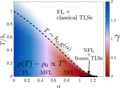
Figure 1: Phase diagram for a system with a linear TLS distribution ($\beta=1$) and $h_{c}/E_{F}=0.4$. $\alpha$ is the dimensionless coupling strength and $h_{c}\ll E_{F}$ is the bare cutoff energy of the TLS distribution. The colored area represents the low-$T$ dynamical regime, characterized for $\alpha<1$ by the exponent $\gamma=2(1-\alpha)$ that governs the inelastic scattering rate. We find FL behavior for $\alpha<1/2$, a MFL at $\alpha=1/2$ and a NFL for $\alpha>1/2$. As $\alpha$ crosses $1$, the TLSs partially freeze at $T=0$, indicated by a thick black line. At temperatures above the renormalized cut off $T>h_{c,R}$, the TLSs act as classical elastic scatterers with $T-$independent scattering rate (plus $T^{2}/E_{F}$ corrections). The crossover to this region is denoted by the fading out of the color.

In this paper we show that a NFL phase can arise due to coupling of electrons to the low-energy two-level excitations of an underlying glassy order. To this end we formulate and solve in a controlled large-$N$ limit a model of $N$ fermion species coupled to $M\sim N$ dynamical two-level systems (TLSs) per site via spatially random interactions. The theory is governed by a non-Gaussian saddle point, which maps to the spin-boson (SB) model. While the electrons constitute an ohmic bath for the TLSs for all coupling strengths, the back action of the TLSs gives rise to a tunable exponent $\gamma(\alpha)$ in the electronic self energy ${\rm Im}\Sigma(\omega)\sim\left|\omega\right|^{\gamma}$. Here $\alpha$ is the dimensionless coupling constant of the problem; see below. Notably, the low-temperature dc resistivity obeys $\rho(T)=\rho_{0}+CT^{\gamma}$, with a tunable exponent $0<\gamma<2$ that depends on the coupling. This behavior offers an alternative viewpoint to the conventional form: $\rho(T)=\rho_{0}+AT+BT^{2}$, that is often used in the interpretation of strange metal behavior Park et al. (2008); Cooper et al. (2009); Doiron-Leyraud et al. (2009); Hussey et al. (2011); Jin et al. (2011); Hussey et al. (2018); Legros et al. (2019); Berben et al. (2022). Our theory draws inspiration from the intricate phase diagrams of high$-T_{c}$ superconductors which often exhibit a competition between multiple frustrated orders that could lead to metallic glassiness Emery and Kivelson (1993); Kivelson and Emery (1998). It is worth noting that such a scenario can arise independently of extrinsic quenched disorder, namely, due to frustration-induced self-generated randomness Schmalian and Wolynes (2000).

We start from the following model of $N$ species of electrons hopping on a $d-$dimensional hypercubic lattice with dispersion $\varepsilon_{\boldsymbol{k}}$. Each site hosts $M$ two-level systems (i.e. spin$-1/2$ Pauli operators) subject to random fields $h_{l,\boldsymbol{r}}$ which we locally describe in their eigenbases:

$$H=\sum_{\boldsymbol{k},i<N}\varepsilon_{\boldsymbol{k}}c_{i\boldsymbol{k}}^{\dagger}c_{i\boldsymbol{k}}-\sum_{\boldsymbol{r},l<M}h_{l,\boldsymbol{r}}\sigma^{z}_{l,\boldsymbol{r}}+H_{\rm int}.$$ (1)

Having multiple TLSs per site ($M\gg 1$) could arise from a coarse grained description of mesoscale collective degrees of freedom of an underlying glassy state Lubchenko and Wolynes (2001, 2003), each of which interacts with many electrons. The coupling between the electrons and TLSs is given by

$$H_{\rm int}=\frac{1}{N}\sum_{\boldsymbol{r},ijl}\boldsymbol{g}_{ijl,\boldsymbol{r}}\cdot\boldsymbol{\sigma}_{l,\boldsymbol{r}}c_{i\boldsymbol{r}}^{\dagger}c_{j\boldsymbol{r}}.$$ (2)

Here, the coupling constants are also assumed to be random numbers. It is natural to add to this problem a term with potential scattering $H_{\rm pot}=\frac{1}{\sqrt{N}}\sum_{\boldsymbol{r},ij<N}V_{ij,\boldsymbol{r}}c_{i\boldsymbol{r}}^{\dagger}c_{j\boldsymbol{r}}$ that induces elastic scattering of the itinerant electrons, while leaving the TLS properties unaffected.

Clearly, for $\boldsymbol{g}_{ijl,\boldsymbol{r}}\sim(0,0,1)$ the TLSs are static and the problem reduces to a single-particle one and can be solved exactly. Electrons cause quantum transitions whenever there are coupling constants that differ from the above choice. We have analyzed the case of general coupling constants and find that the case where $\boldsymbol{g}_{ijl,\boldsymbol{r}}\sim(g_{ijl,\boldsymbol{r}},0,0)$ describes all the important aspects that occur in the generic case Bashan et al. . Finally, we need to specify the distribution function of the random fields and coupling constants. For the latter we chose a Gaussian distribution with zero mean and variance $\overline{g_{ijl,\boldsymbol{r}}g_{ijl,\boldsymbol{r}^{\prime}}}=g^{2}\delta(\boldsymbol{r}-\boldsymbol{r}^{\prime})$. The low-energy collective excitations in a glass are effectively described by a collection of two-level systems (TLS) Anderson et al. (1972); Phillips (1972). Each TLS represents two nearly-degenerate configurations of some local collective mode. The level splitting and tunneling rate, characterizing each TLS, can be considered as independently distributed random variables due to their disordered nature. For the eigenvalues $h$ in Eq. (2) this yields a distribution function ${\cal P}(h)\propto|h|$ for $|h|<h_{c}$, where $h_{c}$ is the maximum splitting of the TLSs, assumed to be much smaller than the Fermi energy, $E_{F}$. In principle, we can consider a more general behavior ${\cal P}_{\beta}(h)\propto|h|^{\beta}$ that also includes the case of a constant distribution for $\beta=0$ (which could describe a physical situation where tunneling is significantly smaller than the energy splitting). We will keep $\beta\geq 0$ arbitrary. The qualitative behavior is, however, similar for all values of $\beta\geq 0$.

In order to solve the problem we employ the formalism developed in the context of Yukawa-SYK models Marcus and Vandoren (2019); Esterlis and Schmalian (2019); Wang and Chubukov (2020); Wang (2020); Wang et al. (2021); Esterlis et al. (2021); Guo et al. (2022); Valentinis et al. (2023a, b); Patel et al. (2023). We start from a coherent-state path integral for the fermions and spin (i.e. TLS) variables, average over the random couplings by using the replica trick, and enforce the identities

$$G_{\boldsymbol{r},\boldsymbol{r}^{\prime}}(\tau,\tau^{\prime})=\frac{1}{N}\sum_{i}\overline{c}_{i\boldsymbol{r}}(\tau)c_{i\boldsymbol{r}^{\prime}}(\tau^{\prime}),$$ (3)

$$\chi_{\boldsymbol{r}}(\tau,\tau^{\prime})=\frac{1}{M}\sum_{l}\sigma_{l,\boldsymbol{r}}^{x}(\tau)\sigma_{l,\boldsymbol{r}}^{x}(\tau^{\prime}),$$ (4)

via corresponding Lagrange multiplier fields $\Sigma_{\boldsymbol{r},\boldsymbol{r}^{\prime}}(\tau,\tau^{\prime})$ and $\Pi_{\boldsymbol{r}}(\tau,\tau^{\prime})$. One can integrate out the fermions and obtains the effective action:

$$S_{\rm eff} = S_{\rm TLS}-N{\rm tr}\log\left(G_{0}^{-1}-\Sigma\right)-N{\rm tr}G\Sigma+\frac{M}{2}{\rm tr}\chi\Pi$$ (5)

$$+ \frac{M}{2}g^{2}\sum_{\boldsymbol{r}}\int_{\tau,\tau^{\prime}}G_{\boldsymbol{r}}\left(\tau,\tau^{\prime}\right)G_{\boldsymbol{r}}\left(\tau^{\prime},\tau\right)\chi_{\boldsymbol{r}}\left(\tau,\tau^{\prime}\right),$$

where the trace is taken over space and time. In contrast to the usual Yukawa-SYK approach, where the role of the TLSs is played by Gaussian bosonic modes, there is no Wick theorem for spin variables and the TLSs cannot be integrated out. Instead, they are governed by the action $S_{\rm TLS}=\sum_{\boldsymbol{r},l}S_{\rm SB}\left[\boldsymbol{\sigma}_{l,\boldsymbol{r}}\right]$ which is a sum of individual spins with fermion-induced dynamics:

$$S_{\rm SB}\left[\boldsymbol{\sigma}_{l,\boldsymbol{r}}\right] = -\int_{\tau,\tau^{\prime}}\Pi_{\boldsymbol{r}}\left(\tau^{\prime}-\tau\right)\sigma_{l,\boldsymbol{r}}^{x}\left(\tau\right)\sigma_{l,\boldsymbol{r}}^{x}\left(\tau^{\prime}\right)$$ (6)

$$- \int_{\tau}h_{l,\boldsymbol{r}}\sigma_{l,\boldsymbol{r}}^{z}(\tau)+S_{\rm Berry}\left[\boldsymbol{\sigma}_{l,\boldsymbol{r}}\right].$$

See Supplementary Information (SI) for details of the derivation of Eq. (6). The last term is merely the Berry phase that occurs from the spin coherent state representation. $S_{\rm SB}\left[\boldsymbol{\sigma}_{l,\boldsymbol{r}}\right]$ is a highly nontrivial local many-body problem. One recognizes easily that it is equivalent to the celebrated spin-boson problem of a localized spin coupled to an environment of bosons with spectral function that leads to the bath function $\Pi_{\boldsymbol{r}}\left(\tau^{\prime}-\tau\right)$ Caldeira and Leggett (1983); Leggett et al. (1987); Costi and Zaránd (1999); Weiss (2012). In our case the bath is due to electronic particle-hole excitations. In the large-$N,M$ limit the theory is governed by the saddle point with respect to to $G$, $\Sigma$, and $\chi$, given respectively by

$$\Sigma_{\boldsymbol{r},\boldsymbol{r}^{\prime}}\left(\tau\right) = \delta_{\boldsymbol{r},\boldsymbol{r}^{\prime}}\frac{M}{N}g^{2}G_{\boldsymbol{r},\boldsymbol{r}}\left(\tau\right)\chi_{\boldsymbol{r}}\left(\tau\right)$$

$$G_{\boldsymbol{r},\boldsymbol{r}^{\prime}}\left(i\omega\right) = \left.\left(G_{0}^{-1}\left(i\omega\right)-\Sigma\left(i\omega\right)\right)^{-1}\right|_{\boldsymbol{r},\boldsymbol{r}^{\prime}}$$

$$\Pi_{\boldsymbol{r}}\left(\tau\right) = -g^{2}G_{\boldsymbol{r},\boldsymbol{r}}\left(\tau\right)G_{\boldsymbol{r},\boldsymbol{r}}\left(-\tau\right).$$ (7)

The saddle with respect to $\Pi$ replaces the right-hand-side of Eq. (4) by its expectation value. Eqs. (7) are similar to the Yukawa-SYK problem, where one obtains essentially a set of coupled Eliashberg equations. The crucial difference is that in our case, $\Pi$ and $\chi$ are not the self energy and propagator of a boson, related by a Dyson equation. Instead $\Pi$ is the bath function of a spin-boson problem whose solution determines $\chi$.

The saddle-point equations (7) together with the solution of the spin-boson problem $S_{\rm SB}$ of (6) are valid for a given disorder configuration $\left\{h_{l,\boldsymbol{r}}\right\}$ of the random field. Hence, the system is not translation invariant and correlation functions like $\left\langle\sigma_{l,\boldsymbol{r}}^{x}\left(\tau\right)\sigma_{l,\boldsymbol{r}}^{x}\left(0\right)\right\rangle$ fluctuate in space. However, to determine the self energy in Eq. (7) we only need to know the average of this correlation function over the $M$ flavors. To proceed we employ the large-$M$ limit to replace sums over the TLS flavors with an average over the TLS splitting distribution: $\frac{1}{M}\sum_{l=1}^{M}\cdots\to\int\mathcal{P}\left(h\right)\cdots dh$. This substitution does not necessitate self-averaging in the replica sense, but rather follows directly from the central limit theorem. Since the distribution is independent of position we obtain a statistical translation invariance for the average of interest. Hence, $\chi(\tau)$ and therefore the bath function $\Pi(\tau)$ are independent of $\boldsymbol{r}$, implying that the local fermionic Green’s function and self energy are position-independent as well.

The theory is therefore governed by a momentum-independent self-energy. Standard manipulations for such a self energy, valid in the regime where the typical bosonic energies are smaller than the electronic bandwidth, yield $\Pi(i\omega)=\frac{\rho_{F}^{2}g^{2}}{2\pi}|\omega|$. That is, the electrons constitute an ohmic bath for the TLSs, independent of the form of the self energy. To proceed, we obtain the TLS-susceptibility $\chi(h_{l},\omega)$ (i.e. for a fixed $h_{l}$) by solving its corresponding SB problem $S_{\rm SB}\left[\boldsymbol{\sigma}_{l,\boldsymbol{r}}\right]$, and average over the random field configurations $\chi(\omega)=\int dh{\cal P}\left(h\right)\chi(h,\omega)$. Then the fermionic self-energy of Eq. (7) can at $T=0$ be written as ${\rm Im}\Sigma_{\rm ret}\left(\omega\right)=-\rho_{F}g^{2}(M/N)\int_{0}^{\left|\omega\right|}d\omega^{\prime}{\rm Im}\chi_{\rm ret}\left(\omega^{\prime}\right)$ (here and henceforth ‘ret’ denotes the retarded function). Extensions to finite temperatures are straightforward.

The solution of the SB model is a classic problem in many-body physics of impurity models Weiss (2012); Leggett et al. (1987). For our purposes we use two established facts: (i) the low-energy physics of the problem is governed by renormalization group equations

$$\frac{d\alpha}{d\ell}=-\alpha\tilde{h}^{2}\,\,\,{\rm and}\,\,\,\frac{d\tilde{h}}{d\ell}=(1-\alpha)\tilde{h}$$ (8)

for the dimensionless coupling constant $\alpha=g^{2}\rho_{F}^{2}/\pi^{2}$ and field $\tilde{h}=h/E_{F}$, where $\ell$ measures the logarithm of the characteristic energy. Its solution yields renormalized fields and coupling constants $h_{R}(h,\alpha)$ and $\alpha_{R}(h,\alpha)$, respectively (up to $\mathcal{O}(1)$ numerical coefficients which can be determined by alternative methods Hur (2008); Camacho et al. (2019); Filyov and Wiegmann (1980); Ponomarenko (1993)). (ii) The correlation function obeys a scaling form in terms of the renormalized field

$${\rm Im}\chi_{\rm ret}(h,\omega,T)=\frac{1}{\omega}f_{\alpha}\left(\frac{\omega}{h_{R}},\frac{T}{h_{R}}\right).$$ (9)

The scaling function $f_{\alpha}$ is known numerically and, in several limiting regimes, analytically. To perform the average over field configurations, it is more convenient to work with the distribution function of renormalized fields:

$${\cal P}_{R,\beta}\left(h_{R}\right)\equiv\frac{dh}{dh_{R}}{\cal P}_{\beta}\left(h\right).$$ (10)

The renormalized distribution function follows from the solution of the flow equations. In Fig. 2 we show the evolution of the corresponding renormalized distribution function as function of coupling constant $\alpha$ for the case of $\beta=1$ (i.e. a linear bare distribution).

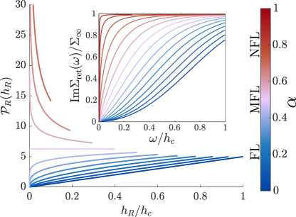
Figure 2: Main: Evolution of the renormalized distribution $\mathcal{P}_{R}(h_{R})$ (see Eq. (10)) is shown for increasing dimensionless coupling $\alpha$ with $\beta=1$ and $h_{c}/E_{F}=0.4$. Inset: Frequency dependence of ${\rm Im}\Sigma_{\rm ret}(\omega)$ at $T=0$ for different $\alpha$. ${\rm Im}\Sigma_{\rm ret}(\omega\ll h_{c,R})\sim|\omega|^{2(1-\alpha)}$, while it saturates to the value $\Sigma_{\infty}\sim\alpha E_{F}$ for $\omega\gg h_{c,R}$ due to the finite Hilbert space of TLSs.

We begin our analysis in the regime $\alpha<1$. In this case the solution of Eqs. (8) yields $h_{R}=E_{F}\tilde{h}^{\frac{1}{1-\alpha}}$Caldeira and Leggett (1983); Leggett et al. (1987); Costi and Zaránd (1999); Weiss (2012), which yields that ${\cal P}_{R,\beta}\left(h_{R}\right)\propto h_{R}^{\beta-\alpha\left(1+\beta\right)}$. The downwards renormalization of the excitation energies of the TLSs leads to a strong weight transfer in the distribution function, making it significantly more singular at low energies. As soon as $\alpha$ reaches $\alpha_{\rm MFL}\equiv\beta/(1+\beta)$ the renormalized distribution function remains finite at arbitrarily small $h_{R}$, for $\alpha>\alpha_{\rm MFL}$ it is even divergent in the low-energy limit. We can now straightforwardly perform the average with the renormalized distribution. We find that at $T=0$, the low-energy ($\omega\ll h_{c,R}$) TLS-susceptibility and the electronic self-energy are characterized by a coupling-constant-dependent exponent $\gamma=(1+\beta)(1-\alpha)$ (see SI for details):

$${\rm Im}\chi_{\rm ret}\left(\omega\right) = {\rm sign}(\omega)\frac{\gamma A_{\alpha}}{h_{c,R}}\left|\frac{\omega}{h_{c,R}}\right|^{\gamma-1},$$

$${\rm Im}\Sigma_{\rm ret}\left(\omega\right) = -\rho_{F}g^{2}A_{\alpha}\frac{M}{N}\left|\frac{\omega}{h_{c,R}}\right|^{\gamma}.$$ (11)

Here, $h_{c,R}$ is the renormalized value of the upper cut-off $h_{c}$. Importantly, the exact form of the scaling function $f_{\alpha}(x,0)$ of Eq. (9) only affects the $\mathcal{O}(1)$ coefficient $A_{\alpha}$, given in the SI. At finite temperatures Eq. (9) implies that the averaged TLS-correlation function and hence the self energy obey $\omega/T$-scaling. Since the exponent $\gamma$ is a continuous function of the coupling strength $\alpha$, the self-energy can be tuned to realize a marginal Fermi-liquid form: ${\rm Im}\Sigma_{\rm ret}\left(\omega\right)\sim|\omega|$, provided that $\alpha=\alpha_{\rm MFL}$. The MFL behavior arises at generic couplings and is not associated with a quantum critical point Sachdev (2011), rather, the system smoothly crosses over between a Fermi liquid for $\alpha<\alpha_{\rm MFL}$, where the lifetime is large compared to the excitation energy, and a non-Fermi liquid for $\alpha>\alpha_{\rm MFL}$.

We proceed to consider transport properties of the theory using the Kubo formula. With vanishing vertex corrections due to spatially uncorrelated interactions, the $T$-dependence of the conductivity follows from the frequency dependence of the self energy. We find

$$\rho(T\ll h_{R,c})-\rho_{0}\propto T^{\gamma},$$ (12)

where the residual resistivity, $\rho_{0}$, is due to the potential scattering term $H_{\rm pot}$. The same reasoning for the thermal conductivity implies that the Wiedemann-Franz law is obeyed in the $T\rightarrow 0$ limit Tulipman and Berg (2022). For $T\gtrsim h_{R,c}$, $\rho(T)$ saturates to a $T-$independent constant, up to a small $T^{2}/E_{F}$ correction. Our results agree with the MFL behavior and corresponding $T$-linear resistivity previously obtained in the weak coupling limit with $\beta=0$ and $\alpha\to 0$ Black et al. (1979). The optical conductivity is given by $\sigma(\Omega)=\sigma_{\rm el}(\Omega)+\sigma_{\rm TLS}(\Omega)$, where the first term denotes the electronic contribution and the second term is due to dipole excitations of TLSs, with magnitude proportional to the typical TLS-dipole moment. At $T=0$, in the absence of potential scatterers we find $\sigma_{\rm el}\propto\Omega^{-{\rm min}(2-\gamma,\gamma)}$ ($\gamma=1$ admits a logarithmic correction $\sim\Omega^{-1}\log^{-2}(\Omega)$), while the TLS term reads $\sigma_{\rm TLS}(\Omega)\propto\overline{d^{2}}\Omega{\rm Im}\chi_{\rm ret}(\Omega)$, $\overline{d^{2}}$ being the typical squared magnitude of the TLS-dipole moment, and hence may give rise to a non-monotonic $\Omega$-dependence of the optical response. The $T$-dependence of the resistivity and the frequency dependence of $\sigma(\Omega)$, with small potential scattering term included, are shown in Fig. 3.

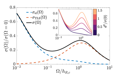
Figure 3: Representative plot of the optical conductivity at the MFL point ($\gamma=1$). The electronic and TLS contributions are shown in dashed lines. Inset shows the total optical conductivity for different values of the TLS-dipole moment strength $d^{2}$.

A similar analysis can be performed for a coupling constant $\alpha=1$ and $\alpha>1$. For $\alpha=1$ the renormalized field is exponentially small, $h_{R}\sim E_{F}\exp\left(-\tfrac{\pi}{2\tilde{h}}\right)$, which yields a renormalized distribution function ${\cal P}_{R}\left(h_{R}\right)\sim h_{R}^{-1}\log^{-(2+\beta)}\left(\frac{E_{F}}{h_{R}}\right)$ and we find for the TLS propagator and fermionic self energy the highly singular behavior

$${\rm Im}\chi_{\rm ret}\left(\omega\right) \sim \frac{1}{\omega\log^{2+\beta}\left(\frac{E_{F}}{\left|\omega\right|}\right)},$$

$${\rm Im}\Sigma_{\rm ret}\left(\omega\right) \sim \frac{1}{\log^{1+\beta}\left(\frac{E_{F}}{\left|\omega\right|}\right)},$$ (13)

where the single-particle scattering rate vanishes extremely slowly as $\omega\rightarrow 0$, a behavior owed to the fact that there are many exponentially small excitations of the ensemble of TLSs (this is reminiciesnt of the behavior found in Giamarchi et al. (1993)).

For $\alpha>1+h/E_{F}$ the flow equations imply that the field $\tilde{h}$ flows to zero and the TLS freezes due to the Caldeira-Leggett mechanism Caldeira and Leggett (1981); Chakravarty (1982); Chakravarty and Leggett (1984); Leggett et al. (1987); Weiss (2012). This yields a contribution $\delta\left(h_{R}\right)$ to the renormalized distribution function and a corresponding term $\sim\delta\left(\omega\right)$ in ${\rm Im}\chi\left(\omega\right)$, giving rise to a constant elastic scattering term in ${\rm Im}\Sigma\left(\omega\right)$. The frozen TLSs behave like additional potential scatterers and give an extra contribution to the residual resistivity, i.e. Fermi liquid behavior is reinstated. In the narrow regime $1<\alpha<1+h_{c}/E_{F}$ we must divide the TLSs into those which are still dynamical ($h/E_{F}>\alpha-1$), and those which are frozen ($h/E_{F}\leq\alpha-1$). While the frozen ones give rise to a constant ${\rm Im}\Sigma_{\rm ret}\left(\omega\right)$, the contribution of the dynamical ones will be similar to that for $\alpha=1$ given in Eq. (13).

In conclusion, we formulated and solved a model for two-level systems coupled to electrons that are expected to emerge in a glassy metallic state. As a result we find a critical phase with exponents that change as one varies non-thermal parameters that influence the dimensionless coupling constant, i.e. that affect the electronic density of states or the interaction matrix element. Electrons form an ohmic bath for the TLS, while the back action of TLSs yields the variable exponent for electrons. We then find a sequence of crossovers from a Fermi liquid via a marginal Fermi liquid and to a non-Fermi liquid state as one increases the coupling strength; once the interaction becomes too strong, all TLSs freeze and one recovers Fermi liquid behavior. We verified that these results are robust if we include more generic coupling constants $\boldsymbol{g}_{ijl,\boldsymbol{r}}$, even though this requires introducing multiple ohmic baths, provided that the dominant bath is not aligned with the direction of the field Bashan et al. (i.e. that the $z$ component of $\boldsymbol{g}^{2}$ is not the largest of the three).

Our model is solvable in the large-$N$,$M$ limit. Physically, this limit may describe the case where the TLSs are spatially extended, and interact with many channels of incident itinerant electrons, each with a random interaction (corresponding to the many electron ‘flavors’ in our model). Nevertheless, it is important to mention how $1/N$ corrections may modify the results at small energies. One effect neglected in our analysis is RKKY-like interactions between TLSs (mediated by itinerant electrons), which are suppressed by $1/N$ due to the frustrated nature of the interactions. Including this effect, we find that each TLS modifies the bath felt by other TLSs Dobrosavljević and Miranda (2005); Tanasković et al. (2005), and its ohmic behavior breaks down below a small energy scale $\omega_{\star}\sim E_{F}/N^{\frac{1}{2-\gamma}}$. Another interesting $1/N$ effect concerns the validity of the self-averaging assertion, which we find to hold only above energies of order $\omega_{\star\star}\sim h_{c,R}/N^{\frac{1}{\gamma}}$. We defer further investigation of such effects to future study Bashan et al. .

Our analysis can be extended to investigate the role of TLS fluctuations for the formation of Cooper pairs. We expect that they will cause or strengthen existing pairing interactions that are particularly pronounced at intermediate coupling. Our theory is applicable in arbitrary space dimensions $d>1$, i.e. the quantum critical phase is not due to strong long-wave fluctuations that are particularly pronounced in low dimensions, but due to the very slow dynamics present in an ensemble of local degrees of freedom. It is conceivable that such slow local fluctuation of a glassy state are responsible for some of the strange metal behavior observed in strongly correlated materials.

Acknowledgements.— This work was motivated and inspired by prior discussions and unpublished work with G. Grissonnanche, S. A. Kivelson, C. Murthy, A. Pandey, B. Ramshaw, and B. Spivak on the physics of two-level systems in electronic glasses and their possible role in strange metals. We also thank N. Andrei, A. V. Chubukov, V. Dobrosavljevic, T. Holder, P. A. Lee, Y. Oreg, S. Sachdev, A. Shnirman and C. Varma for helpful discussions. J.S. was supported by the German Research Foundation (DFG) through CRC TRR 288 “ElastoQMat,” project B01 and a Weston Visiting Professorship at the Weizmann Institute of Science. E.B. was supported by the European Research Council (ERC) under grant HQMAT (Grant Agreement No. 817799) and by the Israel-US Binational Science Foundation (BSF). Some of this work was performed at KITP, supported in part by the National Science Foundation under PHY-1748958.

Appendix A Mapping to the spin-boson model

In this Appendix, we provide further details on the mapping of our model to the spin-boson problem with an ohmic bath (Equations 6, 7 in the main text). We set $V^{2}=0$ for simplicity, as its inclusion makes no difference in the derivation below. We specialize to the case where $\boldsymbol{h}\propto\hat{z},\boldsymbol{g}\propto\hat{x}$, although the derivation of the most general case is essentially the same and will be shown in Bashan et al. .

We begin by considering the spin coherent-state path integral representation for the TLSs. The partition function for a given configuration of $h$ and $g$ is given by

$$Z[h,g]=\int\mathcal{D}[\boldsymbol{\sigma},c,\overline{c}]e^{-S},$$ (14)

with the action $S=S_{0}+S_{\rm int}$:

$$S_{0} = \sum_{\boldsymbol{r}}\sum_{l=1}^{M}S_{\rm Berry}[\boldsymbol{\sigma}_{l,\boldsymbol{r}}]-\sum_{\boldsymbol{r}}\sum_{l=1}^{M}\int_{\tau}h_{l,\boldsymbol{r}}{\sigma}^{z}_{l,\boldsymbol{r}}$$ (15)

$$+ \sum_{i=1}^{N}\sum_{\boldsymbol{k}}\int_{\tau}\overline{c}_{i\boldsymbol{k}}(\partial_{\tau}+\varepsilon_{\boldsymbol{k}})c_{i\boldsymbol{k}},$$

$$S_{\rm int} = \frac{1}{N}\sum_{\boldsymbol{r}}\sum_{i,j=1}^{N}\sum_{l=1}^{M}\int_{\tau}{g}_{ijl,\boldsymbol{r}}{\sigma^{x}}_{l,\boldsymbol{r}}\overline{c}_{i\boldsymbol{r}}c_{j\boldsymbol{r}}.$$ (16)

Here we kept the same symbols $\boldsymbol{\sigma}_{l,\boldsymbol{r}}$ for the unit vectors that result from the coherent state representation of the Pauli operators. $S_{\rm Berry}$ denotes the Berry’s phase of the TLSs, see e.g. Auerbach (1998).

To proceed, we average over the random couplings $g_{ijl,\boldsymbol{r}}$ using the replica method, and introduce the bilocal fields in Eqs. (3) and (4), which we enforce via conjugated fields, $\Sigma$ and $\Pi$, respectively.

Next, we integrate over the fermions and substitute a replica-diagonal Ansatz, which allows us to express the partition function as $Z[h]=\int\mathcal{D}\left[G,{\chi},\Sigma,\Pi,\boldsymbol{\sigma}\right]e^{-S_{\rm eff}}$, where the effective action is given by

$$S_{\rm eff} = -N\text{Tr}\ln\left(G_{0}^{-1}-\Sigma\right)-N\int_{\tau,\tau^{\prime}}\sum_{\boldsymbol{r},\boldsymbol{r}^{\prime}}\sum_{\sigma}G_{\boldsymbol{r},\boldsymbol{r}^{\prime}}\left(\tau,\tau^{\prime}\right)\Sigma_{\boldsymbol{r},\boldsymbol{r}^{\prime}}\left(\tau,\tau^{\prime}\right)+\frac{M}{2}\int_{\tau,\tau^{\prime}}\sum_{\boldsymbol{r}}\chi_{\boldsymbol{r}}\left(\tau,\tau^{\prime}\right)\Pi_{\boldsymbol{r}}\left(\tau^{\prime},\tau\right)$$ (17)

$$+ \frac{M}{2}\int_{\tau,\tau^{\prime}}\sum_{\boldsymbol{r}}g^{2}G_{\boldsymbol{r}}\left(\tau,\tau^{\prime}\right)G_{\boldsymbol{r}}\left(\tau^{\prime},\tau\right)\chi_{\boldsymbol{r}}\left(\tau,\tau^{\prime}\right)+\sum_{\boldsymbol{r}}\sum_{l=1}^{M}S_{\text{Berry}}\left[\boldsymbol{\sigma}_{l,\boldsymbol{r}}\right]-\int_{\tau}\sum_{\boldsymbol{r}}\sum_{l=1}^{M}{h}_{l,\boldsymbol{r}}{\sigma^{z}}_{l,\boldsymbol{r}}$$

$$- \frac{1}{2}\int_{\tau,\tau^{\prime}}\sum_{\boldsymbol{r}}\Pi_{\boldsymbol{r}}\left(\tau^{\prime},\tau\right)\sum_{l=1}^{M}\sigma^{x}_{l,\boldsymbol{r}}\left(\tau\right)\sigma^{x}_{l,\boldsymbol{r}}\left(\tau^{\prime}\right).$$

The limit of large $M$ and $N$, with fixed ratio $M/N$, justifies the use of the saddle point approximation. Performing the variation with respect to $G$ and $\Sigma$ gives the first two lines in Eqs. (7), where we have used thermal equilibrium to write the saddle-point equations with time-translation-invariant correlation functions and their Fourier transforms. In addition, the stationary point that follows from the variation with respect to $\chi$ is

$$\Pi_{\boldsymbol{r}}\left(\tau\right) = -g^{2}G_{\boldsymbol{r},\boldsymbol{r}}\left(\tau\right)G_{\boldsymbol{r},\boldsymbol{r}}\left(-\tau\right).$$ (18)

The Berry phase term $S_{\rm Berry}$, that reflects the fact that no Wick theorem exists for Pauli operators, implies that the TLSs cannot be simply integrated over as a Gaussian integral. However, it allows us to recast the TLS problem to that of $M$ decoupled TLSs per site $\boldsymbol{r}$, $\sum_{\boldsymbol{r},l=1}^{M}S_{\boldsymbol{r},l}\left[\boldsymbol{\sigma}_{\boldsymbol{r},l}\right]$, coupled to a bosonic bath of particle-hole excitations. Each TLS is governed by the spatially local effective action

$$S_{\boldsymbol{r},l}\left[\boldsymbol{\sigma}\right]=S_{{\rm Berry}}\left[\boldsymbol{\sigma}\right]-\int_{\tau}{h}_{l,\boldsymbol{r}}{\sigma^{z}}\left(\tau\right)-\int_{\tau,\tau^{\prime}}\Pi_{\boldsymbol{r}}\left(\tau^{\prime}-\tau\right)\sigma^{x}\left(\tau\right)\sigma^{x}\left(\tau^{\prime}\right).$$ (19)

This is indeed the action of the spin-boson model after the bosonic bath degrees of freedom have been integrated out Weiss (2012) (Eq. 6 in the main text). The latter give rise to the non-local in time coupling $\Pi_{\boldsymbol{r}}^{a}\left(\tau^{\prime},\tau\right)$ that is, in general, different for each site. Of course, in our problem the origin of the bath function are not bosons but the conduction electrons. For the solution of this local problem this makes, however, no difference. $S_{\boldsymbol{r},l}$ still depends on the random configuration ${h}_{l,\boldsymbol{r}}$ of the fields.

For a given realization of the fields ${h}_{l,\boldsymbol{r}}$ the problem is not translation invariant and correlation functions like $\left\langle\sigma_{l,\boldsymbol{r}}^{x}\left(\tau\right)\sigma_{l,\boldsymbol{r}}^{x}\left(0\right)\right\rangle$ fluctuate in space. However, to determine the self energy in the second line of (7) we only need to know the average $\chi_{\boldsymbol{r}}(\tau)$ of this correlation function over the $M$ TLS-flavors. To proceed, we employ the central limit theorem, considering the correlation function $\chi_{\boldsymbol{r}}(\tau)$ as a random variable, we may replace the sum of the TLS flavors with averaging over the TLS splitting distribution ($\sum_{l=1}^{M}\to M\int\mathcal{P}\left({h}_{\boldsymbol{r}}\right)d{h}_{\boldsymbol{r}}$). Since the distribution $\mathcal{P}$ is independent of position, the self-averaging assumption translates to a statistical translation invariance of the model, at least for the average of interest. Hence, $\chi_{\boldsymbol{r}}(\tau)=\chi(\tau)$ is independent on $\boldsymbol{r}$. The same must then hold for the bath function $\Pi_{\boldsymbol{r}}(\tau)=\Pi(\tau)$. From the saddle point equations (18) it follows that the local fermionic Green’s function (and through Eqs. (7), the self energy) are both space independent. Hence we can go to momentum space and find that the theory is goverened by a momentum-independent self-energy and the Dyson equation for the electrons read

$$\Sigma\left(\tau\right) = \frac{M}{N}g^{2}\chi\left(\tau\right)G\left(\tau\right),$$ (20)

$$G_{\boldsymbol{k}}\left(i\omega\right) = \frac{1}{i\omega-\varepsilon_{\boldsymbol{k}}-\Sigma\left(i\omega\right)},$$ (21)

where $G\left(\tau\right)=\int_{\boldsymbol{k}}G_{\boldsymbol{k}}\left(\tau\right)$ is the local Green’s function. For a momentum independent fermionic self energy we obtain in the limit of large electron bandwidth

$$G\left(i\omega\right)=\int_{\boldsymbol{k}}G_{\boldsymbol{k}}\left(i\omega\right)\approx-i\pi\nu_{0}{\rm sgn}\left(\omega\right).$$ (22)

The particle-hole correlation function can now be evaluated. We find

$$\Pi(\omega)=\frac{\nu_{0}^{2}g^{2}}{2\pi}|\omega|,$$ (23)

irrespective of the electronic self-energy. We thus conclude that each TLS is coupled to an ohmic bath of particle-hole excitations that is independent of the back reaction of the TLS on the electronic degrees of freedom. Thus, we have shown that the (spatially local) TLS-correlator

$$\chi\left(\tau-\tau^{\prime}\right) = \frac{1}{M}\sum_{l}\left\langle\sigma_{l}^{x}\left(\tau\right)\sigma_{l}^{x}\left(\tau^{\prime}\right)\right\rangle,$$ (24)

is determined by the behavior of $M$ decoupled SB models.

The strategy of the solution of our model in the large-$N$ limit is therefore: (i) solve the spin-boson problem with ohmic bath for a given realization of the field $\boldsymbol{h}$, (ii) average over the TLS distribution function of the fields, and (iii) use the resulting propagator $\chi_{a}(\omega)$ of the TLSs to determine the fermionic self energy from Eq.(20). The non-linear character of the problem is rooted in the rich physics of the spin-boson problem, along with the averaging over the distribution functions of the fields ${h}$. The dimensionless coupling parameter of the relevant SB model is related to the interaction strengths by:

$$\alpha=\frac{\nu_{0}^{2}g^{2}}{\pi^{2}}.$$ (25)

Appendix B Derivation of Equations 11, 13

At $T=0$, the average (imaginary part of the) susceptibility is given by

$$\overline{\text{Im}\chi_{\rm ret}} = \int_{0}^{h_{c}}\text{Im}\chi_{\rm ret}(\omega,h)\mathcal{P}_{\beta}(h)dh$$ (26)

$$= \int_{0}^{h_{R,c}}\frac{1}{\omega}f_{\alpha}\left(\frac{\omega}{h_{R}},0\right)\mathcal{P}_{R}(h_{R})dh_{R}$$ (27)

$$= {\rm{sgn}}(\omega)\int_{|\omega|/h_{R,c}}^{\infty}\frac{f_{\alpha}\left(x,0\right)}{x^{2}}\mathcal{P}_{R}(|\omega|/x)dx$$ (28)

The result of this integral thus depends on the renormalized distribution $\mathcal{P}_{r}$.

B.1 $\alpha<1$

Starting with $h_{R}=c_{\alpha}\omega_{c}(h/\omega_{c})^{1/(1-\alpha)}\Rightarrow h=(h_{R}/c_{\alpha})^{1-\alpha}\omega_{c}^{-\alpha}$:

$$\mathcal{P}(h_{R}) = \mathcal{P}(h)\left(\frac{dh}{dh_{R}}\right)$$ (29)

$$= \mathcal{N}h_{R}^{\beta(1-\alpha)-\alpha}$$ (30)

Since the distribution is cut off at $h_{R,c}=h_{R}(h_{c})$, the normalization constant must be $\mathcal{N}=\gamma/h_{R,c}^{\gamma}$, with $\gamma=\beta(1-\alpha)-\alpha+1=(1+\beta)(1-\alpha)$. Inserting this into the averaged susceptibility gives:

$$\overline{\text{Im}\chi_{\rm ret}} = {\rm{sgn}}(\omega)\int_{|\omega|/h_{R,c}}^{\infty}\frac{f_{\alpha}\left(x,0\right)}{x^{2}}\frac{\gamma|\omega|^{\gamma-1}}{h_{R,c}^{\gamma}x^{\gamma-1}}dx$$ (31)

$$= \frac{1}{\omega}\left|\frac{\omega}{h_{R,c}}\right|^{\gamma}\times\gamma\int_{|\omega|/h_{R,c}}^{\infty}\frac{f_{\alpha}\left(x,0\right)}{x^{\gamma+1}}dx$$ (32)

Using that fact that at long times $\chi(t)\propto\alpha/t^{2}$, we see that for small frequencies $\text{Im}\chi_{\rm ret}(\omega\ll h_{R})\propto\alpha\omega\Rightarrow f_{\alpha}(x\ll 1)\propto\alpha x^{2}$. Near the lower integration limit the integrand is $\propto 1/x^{\gamma-3}$. If $\gamma<2$ then the integral converges when taking $\omega/h_{R,c}\to 0$, and can thus be considered as a constant of order unity, and we find the frequency dependence $\sim\omega^{\gamma-1}$ as presented in the main text. (If $\gamma>2$ then the integral diverges as $|\omega|^{2-\gamma}$ and the resulting overall frequency dependence is $\overline{\text{Im}\chi_{\rm ret}}\propto\omega$. This is because the averaged susceptibility cannot decay faster than the susceptibility of the TLSs with highest $h$.) Considering Eq. (32), we observe that

$$A_{\alpha}=\int_{0}^{\infty}\frac{f_{\alpha}(x,0)}{x^{\gamma+1}}dx$$ (33)

The scaling function $f_{\alpha}$ is not known analytically for generic values of $\alpha$, but, as previously mentioned, is supported mainly around $x\sim 1$ such that the integral is $\mathcal{O}(1)$. For example at the Toulouse point $A_{1/2}=2$ for a linear distribution.

B.2 $\alpha\approx 1$

In this case we use $h_{R}=c_{\alpha}\omega_{c}\exp(-b\omega_{c}/h)\Rightarrow h=\frac{b\omega_{c}}{2\log\left(\frac{c_{\alpha}\omega_{c}}{h_{R}}\right)}$, which gives the renormalized distribution:

$$\mathcal{P}(h_{R}) = \frac{\mathcal{N}}{h_{R}\log^{2+\beta}\left(\frac{c_{\alpha}\omega_{c}}{h_{R}}\right)}$$ (34)

and the normalization can be found to be $\mathcal{N}=(1+\beta)\log^{1+\beta}(\omega_{c}/h_{R,c})$. We neglect for simplicity the factor of $c_{\alpha}\sim\mathcal{O}(1)$ inside the logarithm. The averaged susceptibility is then given by

$$\overline{\text{Im}\chi_{\rm ret}} = \frac{1+\beta}{\omega}\log^{1+\beta}(\omega_{c}/h_{R,c})\int_{|\omega|/h_{R,c}}^{\infty}\frac{f_{\alpha}\left(x\right)}{x\log^{2+\beta}\left(x\omega_{c}/|\omega|\right)}dx$$ (35)

In order to simplify the integral, we rely on the fact that $f_{\alpha}(x\gg 1)\propto 1/x^{4-2\alpha}$ Guinea (1985) and $f(x\ll 1)\propto x^{2}$, such that most of the weight of the integral is around $x\sim\mathcal{O}(1)$, for which $|\log(x)|\ll\log(\omega_{c}/|\omega|)$. Thus we may neglect the $x$ dependence inside the log and take it out of the integral. We thus retrieve the frequency dependence presented in the main text, and the the $x$ integreal, as before, only affects the numerical prefactor.

References

- Varma (2020) Chandra M. Varma, “Colloquium: Linear in temperature resistivity and associated mysteries including high temperature superconductivity,” Reviews of Modern Physics 92, 031001 (2020).
- Chowdhury et al. (2022) Debanjan Chowdhury, Antoine Georges, Olivier Parcollet, and Subir Sachdev, “Sachdev-Ye-Kitaev models and beyond: Window into non-Fermi liquids,” Reviews of Modern Physics 94, 035004 (2022).
- Hartnoll and Mackenzie (2021) Sean A. Hartnoll and Andrew P. Mackenzie, “Planckian dissipation in metals,” arXiv:2107.07802 (2021).
- Phillips et al. (2022) Philip W. Phillips, Nigel E. Hussey, and Peter Abbamonte, “Stranger than metals,” Science 377, eabh4273 (2022).
- Sachdev (2023) Subir Sachdev, “Quantum statistical mechanics of the Sachdev-Ye-Kitaev model and strange metals,” (2023).
- Proust and Taillefer (2019) Cyril Proust and Louis Taillefer, “The Remarkable Underlying Ground States of Cuprate Superconductors,” Annual Review of Condensed Matter Physics 10, 409–429 (2019).
- Bruin et al. (2013) J. a. N. Bruin, H. Sakai, R. S. Perry, and A. P. Mackenzie, “Similarity of Scattering Rates in Metals Showing T-Linear Resistivity,” Science 339, 804–807 (2013).
- Legros et al. (2019) A. Legros, S. Benhabib, W. Tabis, F. Laliberté, M. Dion, M. Lizaire, B. Vignolle, D. Vignolles, H. Raffy, Z. Z. Li, P. Auban-Senzier, N. Doiron-Leyraud, P. Fournier, D. Colson, L. Taillefer, and C. Proust, “Universal T -linear resistivity and Planckian dissipation in overdoped cuprates,” Nature Physics 15, 142–147 (2019).
- Cao et al. (2020) Yuan Cao, Debanjan Chowdhury, Daniel Rodan-Legrain, Oriol Rubies-Bigorda, Kenji Watanabe, Takashi Taniguchi, T. Senthil, and Pablo Jarillo-Herrero, “Strange Metal in Magic-Angle Graphene with near Planckian Dissipation,” Physical Review Letters 124, 076801 (2020).
- Gegenwart et al. (2008) Philipp Gegenwart, Qimiao Si, and Frank Steglich, “Quantum criticality in heavy-fermion metals,” Nature Physics 4, 186–197 (2008).
- Cooper et al. (2009) R. A. Cooper, Y. Wang, B. Vignolle, O. J. Lipscombe, S. M. Hayden, Y. Tanabe, T. Adachi, Y. Koike, M. Nohara, H. Takagi, Cyril Proust, and N. E. Hussey, “Anomalous Criticality in the Electrical Resistivity of La2–xSrxCuO4,” Science 323, 603–607 (2009).
- Hussey et al. (2018) N. E. Hussey, J. Buhot, and S. Licciardello, “A tale of two metals: contrasting criticalities in the pnictides and hole-doped cuprates*,” Reports on Progress in Physics 81, 052501 (2018).
- Hussey et al. (2013) N. E. Hussey, H. Gordon-Moys, J. Kokalj, and R. H. McKenzie, “Generic strange-metal behaviour of overdoped cuprates,” Journal of Physics: Conference Series 449, 012004 (2013).
- Greene et al. (2020) Richard L. Greene, Pampa R. Mandal, Nicholas R. Poniatowski, and Tarapada Sarkar, “The Strange Metal State of the Electron-Doped Cuprates,” Annual Review of Condensed Matter Physics 11, 213–229 (2020).
- Jaoui et al. (2022) Alexandre Jaoui, Ipsita Das, Giorgio Di Battista, Jaime Díez-Mérida, Xiaobo Lu, Kenji Watanabe, Takashi Taniguchi, Hiroaki Ishizuka, Leonid Levitov, and Dmitri K. Efetov, “Quantum critical behaviour in magic-angle twisted bilayer graphene,” Nature Physics 18, 633–638 (2022).
- Ghiotto et al. (2021) Augusto Ghiotto, En-Min Shih, Giancarlo S. S. G. Pereira, Daniel A. Rhodes, Bumho Kim, Jiawei Zang, Andrew J. Millis, Kenji Watanabe, Takashi Taniguchi, James C. Hone, Lei Wang, Cory R. Dean, and Abhay N. Pasupathy, “Quantum criticality in twisted transition metal dichalcogenides,” Nature 597, 345–349 (2021).
- Pfleiderer (2003) C. Pfleiderer, “Non-Fermi liquid puzzle of MnSi at high pressure,” Physica B: Condensed Matter Proceedings of the Second Hiroshima Workshop on Transport and The rmal Properties of Advanced Materials, 328, 100–104 (2003).
- Pfleiderer et al. (2004) C. Pfleiderer, D. Reznik, L. Pintschovius, H. v Löhneysen, M. Garst, and A. Rosch, “Partial order in the non-Fermi-liquid phase of MnSi,” Nature 427, 227–231 (2004).
- Doiron-Leyraud et al. (2003) N. Doiron-Leyraud, I. R. Walker, L. Taillefer, M. J. Steiner, S. R. Julian, and G. G. Lonzarich, “Fermi-liquid breakdown in the paramagnetic phase of a pure metal,” Nature 425, 595–599 (2003).
- Paschen and Si (2021) Silke Paschen and Qimiao Si, “Quantum phases driven by strong correlations,” Nature Reviews Physics 3, 9–26 (2021).
- Zhao et al. (2019) Hengcan Zhao, Jiahao Zhang, Meng Lyu, Sebastian Bachus, Yoshifumi Tokiwa, Philipp Gegenwart, Shuai Zhang, Jinguang Cheng, Yi-feng Yang, Genfu Chen, Yosikazu Isikawa, Qimiao Si, Frank Steglich, and Peijie Sun, “Quantum-critical phase from frustrated magnetism in a strongly correlated metal,” Nature Physics 15, 1261–1266 (2019).
- Anderson (1995) P W Anderson, “New physics of metals: fermi surfaces without Fermi liquids.” Proceedings of the National Academy of Sciences 92, 6668–6674 (1995).
- Varma et al. (2002) C. M. Varma, Z. Nussinov, and Wim van Saarloos, “Singular or non-Fermi liquids,” Physics Reports 361, 267–417 (2002).
- Lee (2018) Sung-Sik Lee, “Recent Developments in Non-Fermi Liquid Theory,” Annual Review of Condensed Matter Physics 9, 227–244 (2018).
- Varma et al. (1989) C. M. Varma, P. B. Littlewood, S. Schmitt-Rink, E. Abrahams, and A. E. Ruckenstein, “Phenomenology of the normal state of Cu-O high-temperature superconductors,” Physical Review Letters 63, 1996–1999 (1989).
- Sachdev and Ye (1993) Subir Sachdev and Jinwu Ye, “Gapless Spin-Fluid Ground State in a Random Quantum Heisenberg Magnet,” Physical Review Letters 70, 3339–3342 (1993).
-
(27)
Alexei Kitaev, A simple model of quantum holography. http://online.kitp.ucsb.edu/online/entangled15/kitaev/
http://online.kitp.ucsb.edu/online/entangled15/kitaev2/. - Marcus and Vandoren (2019) Eric Marcus and Stefan Vandoren, “A new class of SYK-like models with maximal chaos,” Journal of High Energy Physics 2019, 166 (2019).
- Esterlis and Schmalian (2019) Ilya Esterlis and Jörg Schmalian, “Cooper pairing of incoherent electrons: An electron-phonon version of the Sachdev-Ye-Kitaev model,” Physical Review B 100, 115132 (2019).
- Wang and Chubukov (2020) Yuxuan Wang and Andrey V. Chubukov, “Quantum phase transition in the Yukawa-SYK model,” Physical Review Research 2, 033084 (2020).
- Wang (2020) Yuxuan Wang, “Solvable Strong-Coupling Quantum-Dot Model with a Non-Fermi-Liquid Pairing Transition,” Physical Review Letters 124, 017002 (2020).
- Wang et al. (2021) Wei Wang, Andrew Davis, Gaopei Pan, Yuxuan Wang, and Zi Yang Meng, “Phase diagram of the spin-$\frac{1}{2}$ Yukawa–Sachdev-Ye-Kitaev model: Non-Fermi liquid, insulator, and superconductor,” Physical Review B 103, 195108 (2021).
- Esterlis et al. (2021) Ilya Esterlis, Haoyu Guo, Aavishkar A. Patel, and Subir Sachdev, “Large $N$ theory of critical Fermi surfaces,” Physical Review B 103, 235129 (2021).
- Guo et al. (2022) Haoyu Guo, Ilya Esterlis, Aavishkar A. Patel, and Subir Sachdev, “Large $N$ theory of critical Fermi surfaces II: conductivity,” (2022), 10.48550/arXiv.2207.08841.
- Valentinis et al. (2023a) Davide Valentinis, Gian Andrea Inkof, and Jörg Schmalian, “BCS to incoherent superconductivity crossovers in the Yukawa-SYK model on a lattice,” (2023a).
- Valentinis et al. (2023b) Davide Valentinis, Gian Andrea Inkof, and Jörg Schmalian, “Correlation between phase stiffness and condensation energy across the non-Fermi to Fermi-liquid crossover in the Yukawa-Sachdev-Ye-Kitaev model on a lattice,” (2023b).
- Patel et al. (2023) Aavishkar A. Patel, Haoyu Guo, Ilya Esterlis, and Subir Sachdev, “Universal theory of strange metals from spatially random interactions,” (2023).
- Zaanen (2019) Jan Zaanen, “Planckian dissipation, minimal viscosity and the transport in cuprate strange metals,” SciPost Physics , 061 (2019), arXiv: 1807.10951.
- Hartnoll (2011) Sean A. Hartnoll, “Horizons, holography and condensed matter,” (2011).
- Wú et al. (2022) Wéi Wú, Xiang Wang, and André-Marie Tremblay, “Non-Fermi liquid phase and linear-in-temperature scattering rate in overdoped two-dimensional Hubbard model,” Proceedings of the National Academy of Sciences 119, e2115819119 (2022).
- Park et al. (2008) T. Park, V. A. Sidorov, F. Ronning, J.-X. Zhu, Y. Tokiwa, H. Lee, E. D. Bauer, R. Movshovich, J. L. Sarrao, and J. D. Thompson, “Isotropic quantum scattering and unconventional superconductivity,” Nature 456, 366–368 (2008).
- Doiron-Leyraud et al. (2009) Nicolas Doiron-Leyraud, Pascale Auban-Senzier, Samuel René de Cotret, Claude Bourbonnais, Denis Jérome, Klaus Bechgaard, and Louis Taillefer, “Correlation between linear resistivity and ${T}_{c}$ in the Bechgaard salts and the pnictide superconductor $\text{Ba}{({\text{Fe}}_{1\ensuremath{-}x}{\text{Co}}_{x})}_{2}{\text{As}}_{2}$,” Physical Review B 80, 214531 (2009).
- Hussey et al. (2011) N. E. Hussey, R. A. Cooper, Xiaofeng Xu, Y. Wang, I. Mouzopoulou, B. Vignolle, and C. Proust, “Dichotomy in the T-linear resistivity in hole-doped cuprates,” Philosophical Transactions of the Royal Society A: Mathematical, Physical and Engineering Sciences 369, 1626–1639 (2011).
- Jin et al. (2011) K. Jin, N. P. Butch, K. Kirshenbaum, J. Paglione, and R. L. Greene, “Link between spin fluctuations and electron pairing in copper oxide superconductors,” Nature 476, 73–75 (2011).
- Berben et al. (2022) M. Berben, J. Ayres, C. Duffy, R. D. H. Hinlopen, Y.-T. Hsu, M. Leroux, I. Gilmutdinov, M. Massoudzadegan, D. Vignolles, Y. Huang, T. Kondo, T. Takeuchi, J. R. Cooper, S. Friedemann, A. Carrington, C. Proust, and N. E. Hussey, “Compartmentalizing the cuprate strange metal,” (2022).
- Emery and Kivelson (1993) V. J. Emery and S. A. Kivelson, “Frustrated electronic phase separation and high-temperature superconductors,” Physica C: Superconductivity 209, 597–621 (1993).
- Kivelson and Emery (1998) S. A. Kivelson and V. J. Emery, “Stripe Liquid, Crystal, and Glass Phases of Doped Antiferromagnets,” (1998).
- Schmalian and Wolynes (2000) Jörg Schmalian and Peter G. Wolynes, “Stripe Glasses: Self-Generated Randomness in a Uniformly Frustrated System,” Physical Review Letters 85, 836–839 (2000).
- Lubchenko and Wolynes (2001) Vassiliy Lubchenko and Peter G. Wolynes, “Intrinsic Quantum Excitations of Low Temperature Glasses,” Physical Review Letters 87, 195901 (2001).
- Lubchenko and Wolynes (2003) Vassiliy Lubchenko and Peter G. Wolynes, “The origin of the boson peak and thermal conductivity plateau in low-temperature glasses,” Proceedings of the National Academy of Sciences 100, 1515–1518 (2003).
- (51) Noga Bashan, Evyatar Tulipman, Joerg Schmalian, and Erez Berg, “To appear,” .
- Anderson et al. (1972) P. w. Anderson, B. I. Halperin, and c. M. Varma, “Anomalous low-temperature thermal properties of glasses and spin glasses,” The Philosophical Magazine: A Journal of Theoretical Experimental and Applied Physics 25, 1–9 (1972).
- Phillips (1972) W. A. Phillips, “Tunneling states in amorphous solids,” Journal of Low Temperature Physics 7, 351–360 (1972).
- Caldeira and Leggett (1983) A. O Caldeira and A. J Leggett, “Quantum tunnelling in a dissipative system,” Annals of Physics 149, 374–456 (1983).
- Leggett et al. (1987) A. J. Leggett, S. Chakravarty, A. T. Dorsey, Matthew P. A. Fisher, Anupam Garg, and W. Zwerger, “Dynamics of the dissipative two-state system,” Reviews of Modern Physics 59, 1–85 (1987).
- Costi and Zaránd (1999) T. A. Costi and G. Zaránd, “Thermodynamics of the dissipative two-state system: A Bethe-ansatz study,” Physical Review B 59, 12398–12418 (1999).
- Weiss (2012) Ulrich Weiss, Quantum Dissipative Systems, 4th ed. (WORLD SCIENTIFIC, 2012).
- Hur (2008) K. Le Hur, “Entanglement entropy, decoherence, and quantum phase transitions of a dissipative two-level system,” Annals of Physics 323, 2208–2240 (2008).
- Camacho et al. (2019) Gonzalo Camacho, Peter Schmitteckert, and Sam T. Carr, “Exact equilibrium results in the interacting resonant level model,” Physical Review B 99, 085122 (2019).
- Filyov and Wiegmann (1980) V. M. Filyov and P. B. Wiegmann, “A method for solving the Kondo problem,” Physics Letters A 76, 283–286 (1980).
- Ponomarenko (1993) V. V. Ponomarenko, “Resonant tunneling and low-energy impurity behavior in a resonant-level model,” Physical Review B 48, 5265–5272 (1993).
- Sachdev (2011) Subir Sachdev, Quantum Phase Transitions, 2nd ed. (Cambridge University Press, 2011).
- Tulipman and Berg (2022) Evyatar Tulipman and Erez Berg, “A Criterion for Strange Metallicity in the Lorenz Ratio,” (2022), arXiv:2211.00665.
- Black et al. (1979) J. L. Black, B. L. Gyorffy, and J. Jäckle, “On the resistivity due to two-level systems in metallic glasses,” Philosophical Magazine B 40, 331–334 (1979).
- Giamarchi et al. (1993) T. Giamarchi, C. M. Varma, A. E. Ruckenstein, and P. Nozières, “Singular low energy properties of an impurity model with finite range interactions,” Physical Review Letters 70, 3967–3970 (1993).
- Caldeira and Leggett (1981) A. O. Caldeira and A. J. Leggett, “Influence of Dissipation on Quantum Tunneling in Macroscopic Systems,” Physical Review Letters 46, 211–214 (1981).
- Chakravarty (1982) Sudip Chakravarty, “Quantum fluctuations in the tunneling between superconductors,” Phys. Rev. Lett. 49, 681–684 (1982).
- Chakravarty and Leggett (1984) Sudip Chakravarty and Anthony J. Leggett, “Dynamics of the two-state system with ohmic dissipation,” Phys. Rev. Lett. 52, 5–8 (1984).
- Dobrosavljević and Miranda (2005) V. Dobrosavljević and E. Miranda, “Absence of Conventional Quantum Phase Transitions in Itinerant Systems with Disorder,” Physical Review Letters 94, 187203 (2005).
- Tanasković et al. (2005) D. Tanasković, V. Dobrosavljević, and E. Miranda, “Spin-Liquid Behavior in Electronic Griffiths Phases,” Physical Review Letters 95, 167204 (2005).
- Auerbach (1998) Assa Auerbach, Interacting Electrons and Quantum Magnetism (1998).
- Guinea (1985) F. Guinea, “Dynamics of simple dissipative systems,” Physical Review B 32, 4486–4491 (1985).