Energy-Aware Routing Algorithm for
Mobile Ground-to-Air Charging

Abstract

We investigate the problem of energy-constrained planning for a cooperative system of an Unmanned Ground Vehicles (UGV) and an Unmanned Aerial Vehicle (UAV). In scenarios where the UGV serves as a mobile base to ferry the UAV and as a charging station to recharge the UAV, we formulate a novel energy-constrained routing problem. To tackle this problem, we design an energy-aware routing algorithm, aiming to minimize the overall mission duration under the energy limitations of both vehicles. The algorithm first solves a Traveling Salesman Problem (TSP) to generate a guided tour. Then, it employs the Monte-Carlo Tree Search (MCTS) algorithm to refine the tour and generate paths for the two vehicles. We evaluate the performance of our algorithm through extensive simulations and a proof-of-concept experiment. The results show that our algorithm consistently achieves near-optimal mission time and maintains fast running time across a wide range of problem instances.

I Introduction

Unmanned Aerial Vehicles (UAVs) have become indispensable across a plethora of applications, from surveillance [1] and package delivery [2] to infrastructure inspection[3], environmental monitoring[4], and precision agriculture[5]. Their potential is especially significant for the continuous monitoring of dynamic environments, such as air quality sampling, border security, and the visual inspections of power plants and pipelines. In these persistent surveillance tasks, UAVs are constantly navigating the environment to ensure high-quality and frequent sensing in specified regions. Given this continuous operation, the limited battery life of UAVs becomes a challenging problem, prompting the need for planning optimized for prolonged mission duration.

The battery limitation hampers the overall capabilities of UAVs. To overcome this challenge, a substantial body of research has emerged. Solutions proposed include automated battery swapping mechanisms [6], energy-efficient low-level controllers [7], tactical low-level path planning [8], and charging through Unmanned Ground Vehicles (UGVs) [9]. Alongside, there has been a distinct emphasis on high-level path planning [10, 11], with a focus on energy optimization, especially when integrating UAVs with UGV charging systems. However, many of these efforts overlook the energy demands of the UGVs themselves. Our research aims to rectify this oversight, adopting a comprehensive approach that takes into account the energy requirements of both UAVs and UGVs.

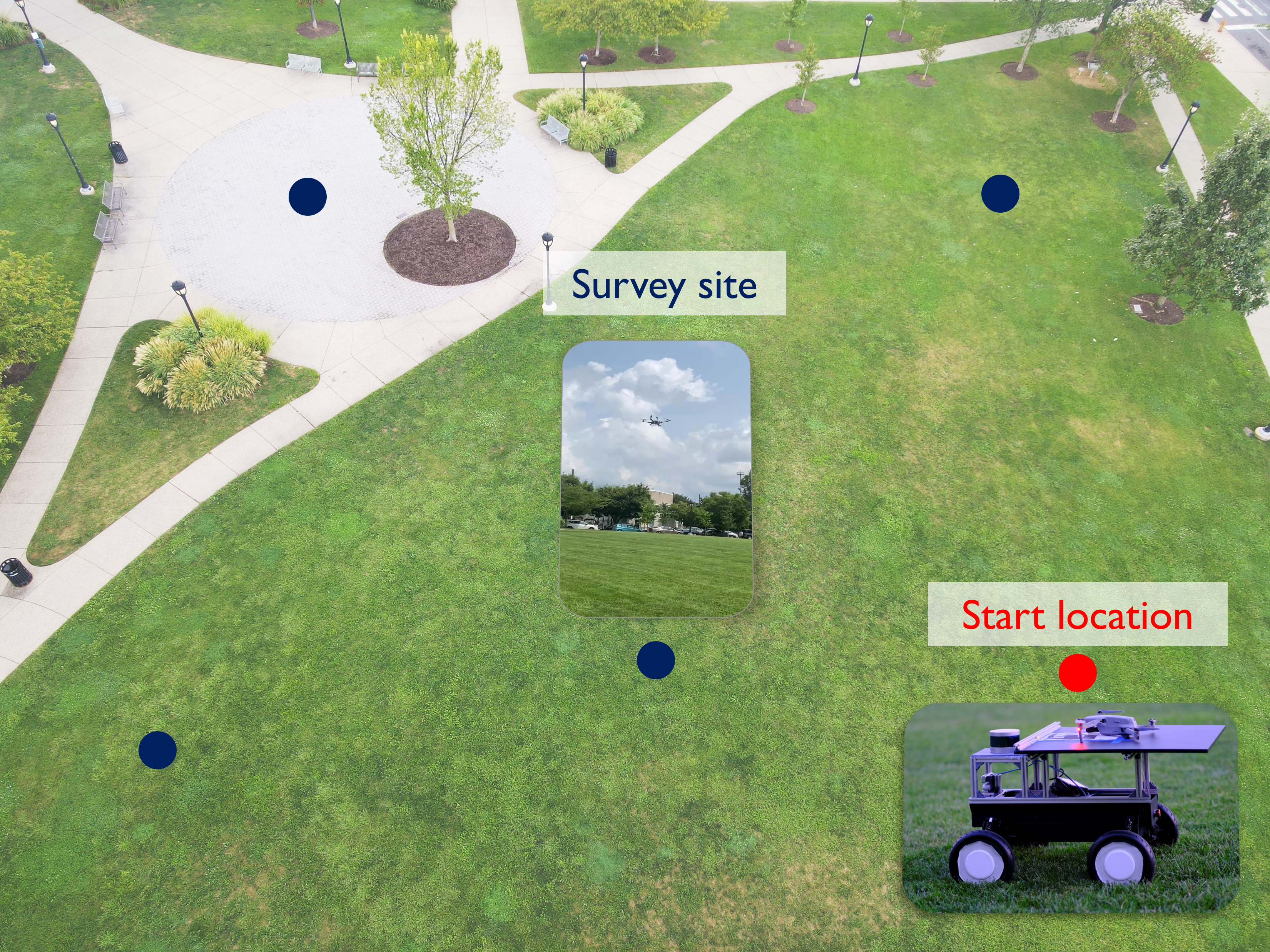
Figure 1: An image of Drexel park with five survey sites (blue dots) scattered on it. A cooperative autonomous platform of an UGV (Segway rover) and an UAV (DJI drone) is tasked to survey these sites.

Specifically, in this paper, we consider an energy-constrained information collection scenario where an UAV is tasked to sequentially survey multiple sites of interest (Fig. 1). Due to its limited battery life, the UAV needs to be charged and/or ferried by a UGV during its mission. We assume that the UGV operates with a fixed battery budget and both vehicles begin their mission from the same location. Our goal is to plan routes for both the UAV and UGV, determining where the UAV should land on the UGV, when the UGV should charge the UAV, and from where the UAV should take off. This is done to ensure the feasibility of the overall task, such as both vehicles being able to return to the starting location, while minimizing the mission time required to survey all sites Most of the previous research on UGV to UAV charging assumes that the UGV has unlimited energy [10, 11, 12]. With this assumption, the path of the UGV can be planned first, and based on that, the path of the UAV is computed. However, we consider energy constraints on both vehicles, which make the problem challenging since the planning for the two vehicles is coupled. To address energy constraints in combined UAV-UGV systems, we introduce an energy-aware routing algorithm combining TSP solutions with the Monte-Carlo Tree Search (MCTS) algorithm. While TSP targets efficient site visits [13], MCTS has proven robust for tree searches [14]. Using the TSP solver, we generate an optimal tour for site surveys. By treating the planning as a tree search, MCTS refines the best routes for both UAV and UGV based on the TSP tour. This integrated approach ensures energy efficiency and optimal mission time.

I-A Related Works

The problem of long-term UAV missions, especially where recharging is a concern, has attracted significant attention in recent literature. This is primarily because of the growing reliance on UAVs for persistent surveillance, delivery, and other applications, necessitating frequent recharges during missions.

One such notable work introduces the concept of employing dedicated charging robots for recharging UAVs during their long-term missions [10]. Their approach is to discretize the UAV’s 3D flight trajectories, projecting them as charging points on the ground. This representation enables an abstraction onto a partitioned graph, from which paths for charging robots are derived. Their methods exploit both integer linear programs and a transformation to the Traveling Salesman Problem (TSP) to craft rendezvous planning strategies.

Another significant contribution to this domain is the exploration of energy-constrained UAV missions, with a focus on minimizing tour time [11]. The authors propose a unique TSP variant that incorporates mobile recharging stations. Their algorithm determines not only the sequence of site visits but also the optimal timings and locations for UAVs to dock on charging stations. They examine multiple charging scenarios, including stationary and mobile charging stations, delivering practical solutions using Generalized TSP.

A more generalized view of persistent surveillance using energy-limited UAVs, supported by UGVs as mobile charging platforms, is presented in [12]. Recognizing the inherent NP-hard nature of this combinatorial optimization problem, the authors suggest a robust approximate algorithm. Their strategy revolves around forming uniform UAV-UGV teams, partitioning the surveillance environment based on UAV fuel cycles, and maintaining cyclic paths that UAVs and UGVs traverse. This research is bolstered by both theoretical findings and practical simulations.

These works collectively highlight the complexities and challenges in planning UAV missions with recharge constraints. However, these studies overlook the energy constraints of the UGVs themselves, a factor that must be considered in real world applications.

I-B Contributions

In this paper, we design and evaluate a novel strategy addressing the intertwined energy and routing challenges in a heterogeneous UAV-UGV system. Our main contributions are as follows.

• Problem formulation: We formulate an energy-constrained routing problem for a cooperative system of an UGV and an UAV to survey multiple sites in a minimal time and under energy constraints for both vehicles.

• Aproach: We design an energy-aware algorithm that integrates a TSP solver to generate an initial guidance tour and then utilizes MCTS to search for the best possible routes for both the UGV and UAV to minimize the total mission time with energy constraints satisfied.

• Results: We conduct both extensive situations and a proof-of-concept experiment to demonstrate the effectiveness and efficiency of our algorithm. The results show that our algorithm generates near-optimal paths for the UGV and UAV and maintains fast running speed even when the number of sites is $50$.

II Problem formulation

Consider an environment with $N$ distinct target sites, we aim to devise a routing strategy for a UAV and UGV pair to survey these sites efficiently. The objective is to minimize the total mission time for sequentially surveying all these sites, and ensuring both vehicles return to their starting point within the energy constraints. We outline relevant notations in Table 1, followed by a detailed discussion on the mission objective, operational dynamics of UGV and UAV, and energy constraints. We then formally present our energy-constrained routing problem.

Symbol	Definition
$E_{\text{Gmax}}$	Maximum energy (i.e., battery capacity) of UGV.
$E_{\text{Amax}}$	Maximum energy (i.e., battery capacity) of UAV.
$e_{\text{g},t}$	The energy of UGV at time $t$.
$e_{\text{a},t}$	The energy of UAV at time $t$.
$C_{\text{a}}$	Flying cost of UAV per kilometer.
$C_{\text{s}}$	Surveying cost of UAV per kilometer.
$C_{\text{g}}$	Moving cost of UGV per kilometer.
$C_{\text{ga}}$	Moving cost of UGV per kilometer when ferrying UAV.
$R_{\text{c}}$	Charging speed in mAh per kilometer.
$V_{\text{a}}$	Speed of UAV.
$V_{\text{g}}$	Speed of UGV.
$T_{\text{survey}}$	Time taken for surveying a site.
$T_{\text{Gwait}}$	Time taken by UGV waiting for UAV for all sites.
$T_{\text{total}}$	Total mission time.

TABLE I: Notations used in the paper

II-A Mission objective

The mission asks for a cooperative system of an UGV and an UAV to survey multiple sites of interest. The UGV serves a dual role—as a mobile base to ferry the UAV and as a mobile charging station to charge the UAV. As the UGV approaches a site, the UAV commences its take-off and heads to surveying the site. Once it completes the survey, it returns and lands on the UGV. This is called one phase of cooperative operation, corresponding to the survey of one site (Fig. 2). Then the next phase starts and the UGV mules the UAV to survey the next site. The same operation continues until all sites are surveyed and the two vehicles return to the start location.

In particular, upon the UAV finishing surveying a site, the two vehicles identify a rendezvous point along the UGV’s path for the UAV to land. We only allow the UGV to arrive earlier at the rendezvous point to wait for the UAV instead of the opposite. That is because, if the UAV arrives earlier and hovers around, it may drain its energy and not be able to land on the UGV anymore, which results in an entire mission failure.

Therefore, the total mission time $T_{\text{total}}$ can be defined as the summation of the UGV’s travel time and the total waiting time it waits for the UAV to return to it after surveying each site. $T_{\text{total}}=\frac{d_{\text{UGV}}}{V_{\text{g}}}+T_{\text{Gwait}}$ where the UGV’s travel time is computed as $d_{\text{UGV}}/V_{\text{g}}$ with $d_{\text{UGV}}$ the distance traveled by UGV. Our primary goal is to minimize the total mission time. In other words, we aim to optimize the efficiency of the UAV-UGV cooperative mission and ensure the timely completion of the survey task.

II-B Cooperative operation for site survey

We introduce in detail a phase of cooperative operation of UGV and UAV. Here, we consider the UAV to have a set of discrete energy amounts based on its current battery level, which follows the same setting for energy management in the previous work [12]. For example, if the UAV’s current battery level is 100%, the set of energy amounts it has can be defined as $[20\%,40\%,60\%,80\%,100\%]$. The UAV can decide how much energy it wants to allocate for surveying a site by selecting an energy amount from the set. This process involves converting the chosen energy amount for the UAV into a range. This range should be sufficient for the UAV to make a round trip from the UGV to the site, as well as to conduct a survey of the site. By doing this conversion, we ensure that after reaching the site and completing its survey, the UAV retains enough energy to land anywhere within a circle, with the site at the center and the computed range as its radius, as shown in Figure 2. The range of the UAV can be determined by subtracting the energy used for the survey from the UAV’s available energy, and then dividing by its per kilometer flying cost $C_{\text{a}}$.

Notably, the mission is to sequentially survey multiple sites of interest, the UAV can decide the energy amount allocated for each site to minimize the total mission time. Please refer to Appendix VI-A for more details.

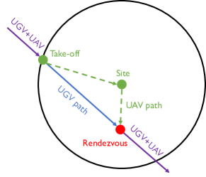
Figure 2: One phase of cooperative operation. The circle is centered at the site and its range is computed based on the UAV’s selected energy amount.

Figure 2 shows one phase of cooperative operation between the UGV and the UAV. The UAV takes off from the UGV (at the blue dot), flies to the site (green dot) for survey, and returns to the UGV at the rendezvous point (red dot). Meanwhile, the UGV moves from the take-off point to the rendezvous point to meet the UAV, and then ferries it to the next take-off point for the next phase.

II-C Energy constraint

We consider the energy constraint for both the UGV and UAV. The UGV is required to not run out of power before returning to the start location. In other words, it must have the energy to return. Notably, the UGV’s energy consumption is contingent upon whether it is ferrying and charging the UAV onboard. During the periods when the UAV necessitates recharging, the UGV allocates its energy to charge the UAV. We assume a recharging efficiency of 100%. This can be easily adjusted according to application contexts by employing a corresponding battery-charging model. While for UAV, since it can be recharged by the UGV, it must be able to return to the UGV for recharging before using up its energy during the entire mission. The violation of either UGV’s or UAV’s energy requirement indicates a mission failure.

In summary, the main problem considered in this paper is to compute the optimal routes for the UGV and UAV to minimize the total mission time (Section II-A) while satisfying all energy constraints (Section II-C). Notably, finding the optimal solutions requires evaluating all possible tours of surveying the sites and all possible combinations of the battery levels across the sites. Clearly, the problem has combinatorial complexity and is NP-hard. To tackle the problem, we design an energy-aware routing algorithm that leverages TSP solution for computing a tour and MCTS for battery level selection in Section III.

III approach

As discussed in Section II, the problem of planning paths for the UGV and UAV with energy constraints is NP-hard. Solving the problem directly is intractable. Therefore, we decompose the problem into two smaller subproblems. Specifically, the first subproblem asks for computing a tour for the two vehicles to efficiently visit and survey all the sites. Subsequently, in the second problem, we focus on allocating the optimal energy amount for the UAV at each site to minimize the total mission time with the energy constraints considered. We develop an energy-aware UGV-UAV routing algorithm that solves these two subproblems in two steps, as shown in Algorithm 1. Next, we introduce Algorithm 1’s two steps in more detail.

III-A The first step of Algorithm 1: TSP

The first step of Algorithm 1 (Line 1) aims to solve the first subproblem that asks for computing a survey tour of all the sites. Given the overall objective is to minimize the total mission time, it is reasonable to seek the shortest tour for the two vehicles. Then, this subproblem can be framed as a TSP problem that entails finding the shortest possible route that visits a list of sites precisely once before returning to the origin. TSP is also NP-hard since computing the optimal tour requires evaluating all possible permutations of the sites, which takes $O(N!)$ time. Fortunately, there exist efficient TSP solvers such as the Google OR-Tools[15], a premier optimization toolkit, that can efficiently determine the optimal tour. Therefore, in the first step, we utilize a TSP solver to compute a shortest tour for the two vehicles, which is outlined in Algorithm 1, line 1 with $\mathcal{X}$ the locations of all sites and $\mathcal{P}$ the generated shortest tour. Notably, the tour generated by the TSP solver provides overall guidance for planning paths for UGV and UAV. However, the actual paths of the two vehicles are generated by also incorporating other factors such as the UAV’s energy allocation at each site, the UAV’s take-off point, the two vehicles’ rendezvous point, etc.

1

// Solve TSP to generate a tour

2 $\mathcal{P}=\texttt{TSP-solver}(\mathcal{X}$)

// MCTS for energy allocation

3 Create root node $v_{0}$

4 while Maximum number of iterations not reached do

       // MCTS selection

5       $v_{i}\leftarrow\texttt{UCB\_Selection}~{}(\text{Tree},v_{0})$

6       if $\operatorname{level}(v_{i})<$ terminal and $m(v_{i})=0$  then

             // MCTS expansion

7            

8            Tree $\leftarrow$ Expand (Tree, $v_{i}$, Energy amounts)

9            if already expanded then

10                  continue

11             end if

12            

13      else

             // MCTS rollout

14             $C\leftarrow\texttt{Rollout}~{}(v_{i})$;

15            

16       end if

      // MCTS backpropagation

17        while $v_{i}\neq\mathrm{NULL}$ do

             // Update rewards and counts

18             $\alpha(v_{i})\leftarrow\alpha(v_{i})+\alpha$

19             $n(v_{i})\leftarrow n(v_{i})+1$

20             $v_{i}\leftarrow$ parent of $v_{i}$

21       end while

22       $M\leftarrow M+1$

23 end while

Path$\_$Generation ($v,\mathcal{P}$)

Algorithm 1 Energy-aware UGV-UAV routing

III-B The second step of Algorithm 1: MCTS

The second step of Algorithm 1 focuses on solving the second subproblem that asks for computing the best energy allocation for the UGV across each site (Lines 1 - 1). Algorithm 1’s first step generates a tour that specifies the order of surveying the sites. Since we consider the discrete energy amounts for the UAV and the sites are surveyed in sequential order, the second subproblem can be treated as a tree search problem where we select an energy amount for the UAV at each tree level. The depth of the tree depends on the number of sites. Clearly, this tree search problem is also NP-hard, which requires evaluation of all possible combinations of the UAV’s energy amounts along the TSP tour to find the optimal solution. One optimal solution could be the depth-first search (DFS) algorithm. However, the exponential growth of the tree makes the DFS algorithm not practical when the number of sites and the number of energy amounts become large.

Instead, we utilize the Monte Carlo Tree Search (Algorithm 1, lines 1 - 1). It has been shown that MCTS is an efficient algorithm that finds near-optimal solutions for tree search problems [16, 17]. To this end, we employ MCTS to find the best energy allocation at each site such that the total mission time is minimized and the energy constraints of the vehicles are satisfied. Next, we introduce the tree structure, pruning strategies, and the MCTS algorithm in detail.

III-B1 Tree structure

The tree starts at a root node, which denotes the commencement location for the cooperative system of the UGV and UAV. The root node also stores the initial energy reserves for the two vehicles, setting the stage for subsequent energy-aware planning. The tree’s child nodes capture possible energy allocation options for the UAV at a particular site. Each child node represents a different energy allocation at a site. For instance, if the UAV can allocate $[20\%,40\%,60\%]$ of its remaining energy, three distinct child nodes (or branches) are spawned and each corresponds to one of the three energy percentages. Recall that each energy amount corresponds to a range or a circle with the site as the center and the range as the radius (Section II-B). That way, each node also represents a certain range for a site. As the UAV and UGV progress through sites, the cumulative influence of prior energy allocations becomes apparent in ensuing branches, progressively restricting future choices due to waning energy reserves. In addition, every node stores data such as elapsed mission time, remaining energy for UGV and UAV, and the energy allocated.

III-B2 Tree pruning

Tree pruning serves as a method to speed up tree search. It reduces computational demands and emphasizes paths that are both feasible and optimal. We introduce the two pruning strategies as follows.

Optimality-based pruning

Once a tree trajectory has been completely traversed, it denotes the attainment of a feasible, albeit not necessarily globally optimal plan. The total time taken is recorded. If, in subsequent explorations, the current node’s cumulative time already surpasses this recorded minimum before the tree is fully expanded, then this node and its children are deemed sub-optimal and are consequently pruned from further consideration. This method aids in circumventing paths that are likely to be less efficient than those already discovered.

Constraint-based pruning

During the tree expansion phase, if a node suggests that either the UAV or UGV has depleted its energy reserve, such a node, along with its subsequent child nodes, is pruned and not included in further exploration. This approach ensures that only scenarios where both vehicles retain operational energy are pursued.

III-B3 MCTS

Traversing the tree entails making iterative selections of possible energy allocations. This process begins by selecting a node and then expanding it. Subsequently, we proceed by randomly progressing through the respective child nodes until an end-point is reached. Once this end-point is achieved, both the reward and visit count are updated, tracing back to the tree’s root. This traversal process can be categorized into four distinct stages: selection, expansion, rollout, and backpropagation. We will go into each of these stages in detail.

Selection (Algorithm 1, line 1)

In the section step, we use the Upper Confidence Bound (UCB) value as a guiding principle to choose an energy allocation for the UAV. It balances the tradeoff between the exploration of new nodes of energy allocation and the exploitation of already visited nodes. Particularly, in the UCB formula (1)

$$\text{UCB}(v_{i})=\frac{\alpha(v^{\prime})}{n(v^{\prime})}+\texttt{const}\sqrt{\frac{2\ln N}{n(v^{\prime})}},$$ (1)

$\text{UCB}(v_{i})$ is the Upper Confidence Bound for a particular energy allocation node $v_{i}$, representing a certain UAV energy amount allocated, $\alpha(v^{\prime})$ is the reward calculated from the total time for the child node $v^{\prime}$, $n(v^{\prime})$ denotes the number of times the child node $v^{\prime}$ has been visited, $N$ denotes the cumulative number of times the parent node $v_{i}$ has been visited, and const is a predefined constant that fine-tunes the balance between exploration of new allocations and exploitation of previously identified allocations.

Expansion (Algorithm 1, lines 1- 1)

Upon selecting a node using the UCB formula, the next step is expansion. Specifically, the selected node is expanded based on the available energy allocation options. For instance, if there exist three energy amounts, and the remaining energy of both UAV and UGV permits, the chosen node will yield three children. Notably, this expansion for a particular node occurs only once.

Rollout (Algorithm 1, line 1)

After the expansion, the rollout process begins. In this phase, child nodes are randomly selected for simulation until a terminal state in the tree is encountered. Notably, if the energy criteria are not satisfied during the rollout, the simulation stops early. To prevent repeated selections of this suboptimal path in future iterations, the visit count of this problematic node is incremented.

Backpropagation (Algorithm 1, lines 1-1)

Upon reaching a terminal state, a reward is determined based on the total time spent. The reward, denoted as $\alpha$, is defined as the inverse of the total time multiplied by a tuneable factor $K>0$. $\alpha=\frac{K}{T_{\text{total}}}$ Then the reward $\alpha$ is propagated back up the tree root, updating both the rewards and visit counts for the traversed nodes.

III-C Path generation for UGV and UAV

The MCTS generates a combination of energy amounts or ranges for the UAV across all sites. Combined with the generated TSP tour, these ranges can be decoded to paths for both the UAV and UGV (as outlined in Algorithm 1, line 1). By integrating this with the TSP tour, $\mathcal{P}$, we can pinpoint the entry and exit locations of the UGV at each circle (Fig. 2), consequently shaping a chord path within the circle. More details are presented in Appendix VI-B. By factoring in their speed differentials and the survey time, we can calculate the UGV’s position on the chord after the UAV’s survey completion. Using all the information above, we can compute the meeting point of the two vehicles on the chord. Thus, the paths for both the UAV and UGV can be determined.

Charging is presumed to initiate immediately upon the UAV’s landing on the UGV. The amount of charge is determined as the minimum among the potential charge, the UAV’s energy deficiency, and the UGV’s energy capacity. This is formally defined by $min\{R_{\text{c}}d_{\text{UAV+UGV}},E_{\text{Amax}}-e_{\text{a},t},e_{\text{g},t}\}$. We present the details in Appendix VI-C.

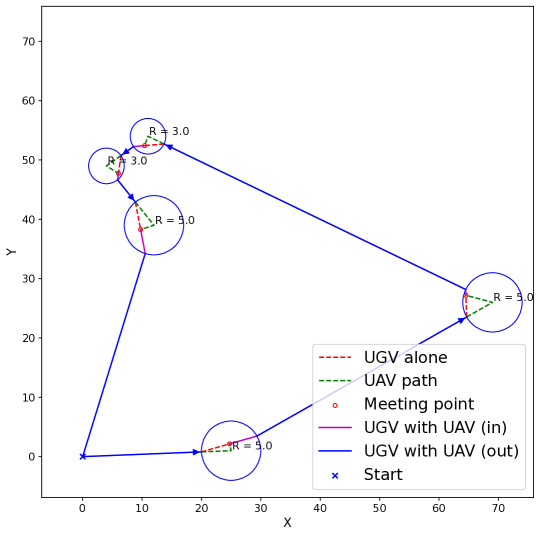
(a) Algorithm 1, $N=5$, $T_{\text{total}}=19.27$ h, $T_{\text{run}}=0.18$ s.

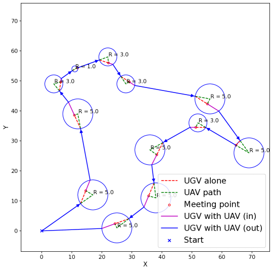
(b) Algorithm 1, $N$ = 12, $T_{\text{total}}=22.33$ h,$T_{\text{run}}=0.52$ s.

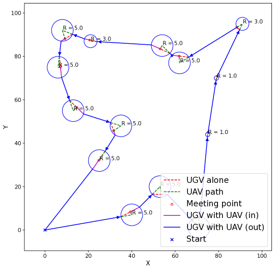
(c) Algorithm 1, $N=14$ , $T_{\text{total}}=37.21$ h, $T_{\text{run}}=0.58$ s.

(d) Brute force, $N=5$ , $T_{\text{total}}$=19.27 h, $T_{\text{run}}=0.6$ s.

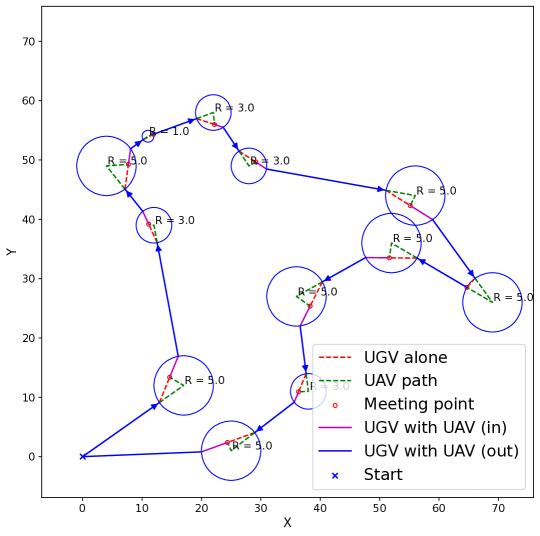
(e) TSP+DFS, $N=12$ , $T_{\text{total}}$ = 22.21 h, $T_{\text{run}}=13.43$ s.

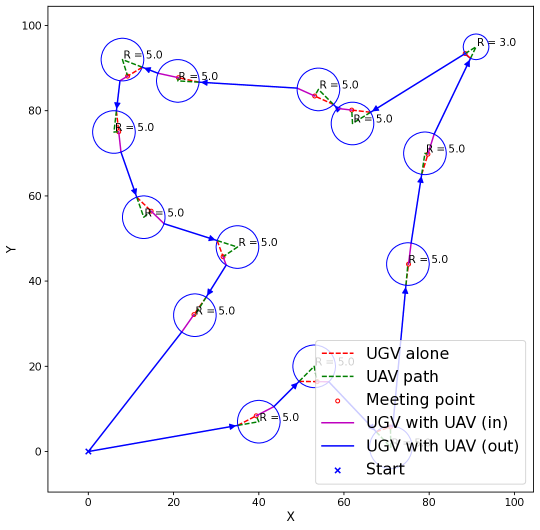
(f) TSP+DFS, $N=14$ , $T_{\text{total}}$ = 37.19 h, $T_{\text{run}}=162.45$ s.

Figure 3: Qualitative comparison of the tour generated by Algorithm 1 with those generated by Brute force and TSP+DFS across $N=5,12,14$ sites.

IV Results

This section presents both qualitative and quantitative results to demonstrate the effectiveness and efficiency of our energy-aware routing algorithm (Algorithm 1). Specifically, we compare Algorithm 1 to three other baseline algorithms. The first algorithm is a brute force algorithm that exhaustively enumerates all possible tours of surveying sites and all possible combinations of the UAV’s energy allocations across sites to find the optimal solution. The second algorithm integrates the TSP solution (Algorithm 1’s first step) to find a shortest tour and the DPS algorithm to find the best combination of the UAV’s energy allocations. We name it TSP + DFS algorithm. Notably, both the brute-force and TSP + DPS algorithms run in exponential time, thus not applicable for large-scale instances. To evaluate the performance of Algorithm 1 with a large number of sites and energy amounts, we compare it to the third algorithm, named naive algorithm. In the naive algorithm, the UGV transports the UAV to each site and waits on-site while the UAV conducts the survey. All evaluations are performed on a Linux desktop with Ubuntu 20.04 powered by an AMD Ryzen 5600X processor with 32GB RAM.

IV-A Qualitative results

We first present qualitative results to evaluate the performance of Algorithm 1 across three different site numbers, i.e., $N=5,12,14$ in Figure 3. Figure 3-(a), (b), (c) shows that Algorithm 1 effectively plans paths for the UGV and UAV by first generating a TSP tour and then allocating energy amounts (or ranges) at each site using MCTS. Comparing to Figure 3-(d), (e), (f), we observe that the paths generated by Algorithm 1 are close to those generated by the brute force algorithm with $N=5$ (Figure 3-(d)), TSP + DSP algorithm with $N=12$ (Figure 3-(e)), and TSP + DSP algorithm with ($N=14$ Figure 3-(f)). In addition, Algorithm 1 performs on par with brute force and TSP + DSP in terms of the mission time $T_{\text{total}}$, but runs much faster. Especially, when $N=14$, the runtime $T_{\text{run}}$ of Algorithm 1 (0.58 s) is more than 280 times less than that of TSP + DSP (162.45 s).

Real robot experiment:. We also run a proof‐of‐concept field experiment to demonstrate the effectiveness of Algorithm 1. Our cooperative autonomous system consists of a customer-designed Segway rover and a commercial DJI drone. The mission of the two vehicles is to survey five sites in Drexel Park (Figure 1). A video of the experiment is available online.

IV-B Quantitative results

We further evaluate Algorithm 1 through quantitative comparisons with other baseline algorithms. Particularly, in small-scale instances with a small number of sites $N\in[2,\cdots,10]$, we compare Algorithm 1 to brute force and TSP + DSP, shown in Figure 4. When the number of sites increases to a large number, brute force and TSP + DSP become inapplicable. Then, we compare Algorithm 1 to the naive algorithm with $N\in[10,\cdots,50]$, as shown in Figure 5.

The small-scale comparison, as shown in Figure 4 further demonstrates that Algorithm 1 archives almost the same mission time but runs much faster than both brute force and TSP + DSP, especially when $N>5$. It is also observed that TSP + DSP performs close to brute force, which justifies the use of the TSP solver to first compute a guided tour for the UGV and UAV.

In the large-scale comparison, Algorithm 1 consistently outperforms the naive algorithm. Particularly, when the number of sites $N=50$, Algorithm 1 archives a mission time that is 15.18 h less that of naive. In addition, even with $N=50$, Algorithm 1 runs less than 0.325 s to generate paths for UGV and UAV.

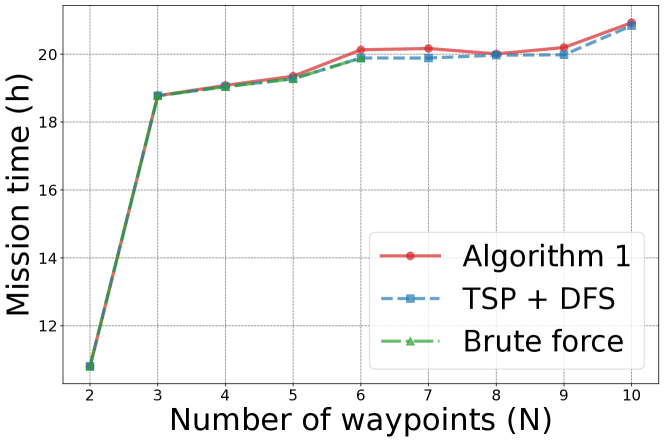
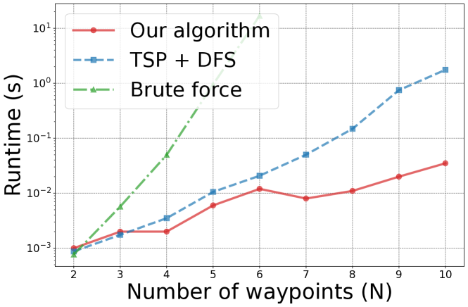
Figure 4: Quantitative composition of Algorithm 1 with brute force and TSP + DSP in terms of mission time $T_{\text{total}}$ and runtime $T_{\text{run}}$ in small scale cases. The y-axis is in log scale. brute force stops at six sites due to its prohibitively long runtime when $N>6$.

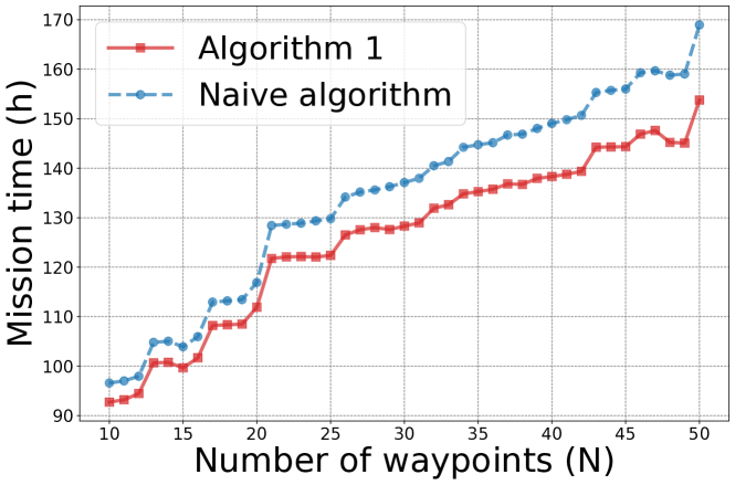
Figure 5: Quantitative composition of Algorithm 1 with naive and in terms of mission time $T_{\text{total}}$ and runtime $T_{\text{run}}$ in large scale cases. The y-axis is in log scale.

V Conclusion and Future Directions

In our exploration of UAV-UGV cooperative missions, we introduced a planning methodology attuned to the energy budgets of both aerial and ground units. In scenarios where the UGV serves as both a transporter and a charging station for the UAV, our algorithm incorporates TSP to determine an initial tour and employs MCTS to refine the routes for both UGV and UAV. We evaluated the performance of our algorithm thorough simulations and experiments. Our findings demonstrated the algorithm’s efficiency across a diverse range of instance sizes and its consistent production of near-optimal solutions.

An ongoing work is to refine our algorithm by merging the survey of nearby sites. This might change the structure of our decision tree but could provide performance gains on the total mission time. The second future work is to design an online routing algorithm based on our current offline algorithm, to offer real-time adaptability, catering to dynamically changing and uncertain environments.

VI Appendix

We first introduce the methodology to convert energy allocation to radius. Then we describe the process of transforming the TSP tour into UGV routing. Finally, we present the calculation of the rendezvous point for the UGV and UAV.

VI-A Convert energy allocation to radius

Given an energy allocation of the UAV, $e_{\text{a}}\in\{10\%\cdot E_{\text{Amax}},20\%\cdot E_{\text{Amax}},\ldots,100\%\cdot E_{\text{Amax}}\}$, the radius can be calculated by

$$r=\frac{{e_{a}-C_{\text{s}}}}{C_{\text{a}}}.$$ (2)

Notably, each energy allocation corresponds to the radius of a circle where the UAV can complete a round trip between any point on the circle and the circle’s center plus the survey at the center by using the allocated energy.

VI-B Covert TSP to UGV routing path

The TSP solver generates a survey tour, determining the sequence of sites to be visited. This sequence can then be converted into a feasible UGV path. As shown in Figure 6, the UGV path is initialized by connecting all the sites using the TSP tour, i.e., $S\rightarrow O_{1}\rightarrow O_{2}\rightarrow O_{3}\rightarrow S$. Recall that each site corresponds to a circle centered at the site and with the radius converted from the energy allocated. The UGV path is then computed as the polyline from the start location to each intersection of the circles with the initialized path, and finally back to the start location, i.e., $S\rightarrow A_{1}\rightarrow B_{1}\rightarrow A_{2}\rightarrow B_{2}\rightarrow A_{3}\rightarrow B_{3}\rightarrow S$.

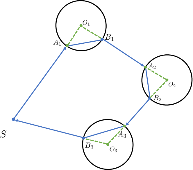
Figure 6: An illustration of transforming the TSP tour $S\rightarrow O_{1}\rightarrow O_{2}\rightarrow O_{3}\rightarrow S$ into the UGV path $S\rightarrow A_{1}\rightarrow B_{1}\rightarrow A_{2}\rightarrow B_{2}\rightarrow A_{3}\rightarrow B_{3}\rightarrow S$.

VI-C Calculate the rendezvous point

We leverage the following definitions to calculate the rendezvous point.

Symbol	Definition
$r$	The radius of the circle.
$O$	The center of the circle.
$AB$	The chord that UGV traverses.
$S$	The distance from $A$ where the UGV starts.
$P$	The point where the UAV and UGV rendezvous.
$M$	The midpoint of the chord $AB$.

Figure 7: Calculation of the survey radius and rendezvous point of the UAV and UGV at a site. The circle is centered at site $O$ with radius $r$. $A$ and $B$ are endpoints of the chord where the UGV traverses, with $M$ as its midpoint. The UAV takes off from $A$ and meets the UGV at $P$. $A\to O\to P$ denotes the flight path of the UAV. $MO$ is an auxiliary line perpendicular to chord $AB$.

As shown in Figure 7, to calculate rendezvous point $P$ located on $AB$, we set the unknowns to be $MP$ and $OP$. Given $M$ is the middle point of the chord $AB$, the triangle $OMP$ is right-angled at $M$. Then we have

$$MP^{2}=OP^{2}-OM^{2},$$

and

$$MP=\sqrt{OP^{2}-OM^{2}}.$$ (3)

As $AO$ (the radius) and $AB$ (from the TSP tour) are known, we compute $OM$ by

$$OM=\sqrt{r^{2}-\left(\frac{AB}{2}\right)^{2}}.$$ (4)

Substituting Equation 4 into Equation 3, we obtain

$$MP=\sqrt{OP^{2}+\left(\frac{AB}{2}\right)^{2}-r^{2}}.$$ (5)

In addition, for the UGV and UAV to meet at point $P$, the time that each vehicle spends to arrive at $P$ from $A$ is equal. The UAV travels for $(AO+OP)/{V_{\text{a}}}$ time (with $AO=r$) along its path $A\to O\to P$ and takes $T_{\text{survey}}$ time for survey at $O$. In total, it spends $(r+OP)/{V_{\text{a}}}+T_{\text{survey}}$ to reach $P$. The UGV spends $AP/V_{\text{g}}=(AM+MP)/V_{\text{g}}=(AB/2+MP)/V_{\text{g}}$ to reach $P$. Making these two times equal, we have

$$\frac{r+OP}{V_{\text{a}}}+T_{\text{survey}}=\frac{AB/2+MP}{V_{\text{g}}}.$$ (6)

Now, we can use Equations 5 and 6 to solve for two unknowns $MP$ and $OP$. Once we have either $MP$ and $OP$, we can calculate the coordinates of point $P$ since the coordinates of $A$, $B$, $M$, and $O$ are known.

Notably, depending on the speeds of the UGV and UAV, there may be cases where the UGV must wait for the UAV at point $B$, introducing a waiting time that must be incorporated into the total mission time, $T_{\text{total}}$.

References

- [1] D. Kingston, R. Beard, and R. Holt, “Decentralized perimeter surveillance using a team of uavs,” IEEE Trans. Robot., vol. 24, no. 6, pp. 1394–1404, Dec 2008.
- [2] N. Mathew, S. L. Smith, and S. L. Waslander, “Planning paths for package delivery in heterogeneous multirobot teams,” IEEE Transactions on Automation Science and Engineering, vol. 12, no. 4, pp. 1298–1308, 2015.
- [3] M. Burri, J. Nikolic, C. Hürzeler, J. Rehder, and R. Siegwart, “Aerial service robots for visual inspection of thermal power plant boiler systems,” in Proc. 2nd Int. Conf. Appl. Robot. Power Ind., 2012, pp. 70–75.
- [4] J. A. D. E. Corrales, Y. Madrigal, D. Pieri, G. Bland, T. Miles, and M. Fladeland, “Volcano monitoring with small unmanned aerial systems,” in Amer. Inst. Aeronautics Astronautics Infotech Aerosp. Conf., Garden Grove, CA, USA, 2012.
- [5] A. Ribeiro and J. Conesa-Muñoz, “Multi-robot systems for precision agriculture,” Innovation in Agricultural Robotics for Precision Agriculture: A Roadmap for Integrating Robots in Precision Agriculture, pp. 151–175, 2021.
- [6] D. Lee, J. Zhou, and W. T. Lin, “Autonomous battery swapping system for quadcopter,” in 2015 International Conference on Unmanned Aircraft Systems (ICUAS), 2015, pp. 118–124.
- [7] D. Palossi, M. Furci, R. Naldi, A. Marongiu, L. Marconi, and L. Benini, “An energy-efficient parallel algorithm for real-time near-optimal uav path planning,” in Proceedings of the ACM International Conference on Computing Frontiers, 2016, pp. 392–397.
- [8] M. Chodnicki, B. Siemiatkowska, W. Stecz, and S. Stepień, “Energy efficient uav flight control method in an environment with obstacles and gusts of wind,” Energies, vol. 15, no. 10, p. 3730, 2022.
- [9] A. Bin Junaid, A. Konoiko, Y. Zweiri, M. N. Sahinkaya, and L. Seneviratne, “Autonomous wireless self-charging for multi-rotor unmanned aerial vehicles,” energies, vol. 10, no. 6, p. 803, 2017.
- [10] N. Mathew, S. L. Smith, and S. L. Waslander, “Multirobot rendezvous planning for recharging in persistent tasks,” IEEE Transactions on Robotics, vol. 31, no. 1, pp. 128–142, 2015.
- [11] K. Yu, A. K. Budhiraja, S. Buebel, and P. Tokekar, “Algorithms and experiments on routing of unmanned aerial vehicles with mobile recharging stations,” Journal of Field Robotics, vol. 36, no. 3, pp. 602–616, 2019.
- [12] X. Lin, Y. Yazıcıoğlu, and D. Aksaray, “Robust planning for persistent surveillance with energy-constrained uavs and mobile charging stations,” IEEE Robotics and Automation Letters, vol. 7, no. 2, pp. 4157–4164, 2022.
- [13] M. Jünger, G. Reinelt, and G. Rinaldi, “The traveling salesman problem,” Handbooks in operations research and management science, vol. 7, pp. 225–330, 1995.
- [14] T. Dam, G. Chalvatzaki, J. Peters, and J. Pajarinen, “Monte-carlo robot path planning,” IEEE Robotics and Automation Letters, vol. 7, no. 4, pp. 11 213–11 220, 2022.
- [15] L. Perron and V. Furnon. Or-tools. Google. [Online]. Available: https://developers.google.com/optimization/
- [16] B. Kartal, E. Nunes, J. Godoy, and M. Gini, “Monte carlo tree search for multi-robot task allocation,” in Proceedings of the AAAI Conference on Artificial Intelligence, vol. 30, no. 1, 2016.
- [17] C. B. Browne, E. Powley, D. Whitehouse, S. M. Lucas, P. I. Cowling, P. Rohlfshagen, S. Tavener, D. Perez, S. Samothrakis, and S. Colton, “A survey of monte carlo tree search methods,” IEEE Transactions on Computational Intelligence and AI in games, vol. 4, no. 1, pp. 1–43, 2012.