The role of the species scale as the Quantum Gravity (QG) cut-off has been recently emphasised in the context of the Swampland Program. Along these lines, we continue the quest for a global definition of the species scale within the moduli spaces of QG by exploiting duality symmetries, the known asymptotic behaviours imposed by the presence of infinite towers of light states, as well as the known behaviour of higher curvature corrections to the Einstein-Hilbert action in certain String Theory set-ups. In those cases, we obtain a consistent result for the identification of the (global) species scale as the Quantum Gravity cut-off, but also present some puzzles related to the suppression of higher-dimensional corrections and certain minor ambiguities that may arise in the deep interior of moduli space.

1 Introduction

The goal of the Swampland Program [1] (see also [2, 3, 4, 5, 6, 7, 8] for reviews) is to distinguish the set of EFTs that can be consistently coupled to Quantum Gravity (QG) from those that cannot. In particular, the main focus is put on gravitational EFTs that reduce to Einstein gravity coupled to matter in the infra-red (IR), but it must be emphasised that the fact that they are merely EFTs can be translated into the existence of (generically) infinite towers of higher-dimensional operators that are suppressed at low energies. Thus, one expects the following schematic form of the EFT action in $D$ spacetime dimensions

$$S_{\mathrm{EFT,\,}D}=\int d^{D}x\ \dfrac{1}{2\kappa_{D}^{2}}\left(\mathcal{R}+\sum_{n}\frac{\mathcal{O}_{n}(\mathcal{R})}{\Lambda_{\text{QG}}^{n-2}}\right)+\ldots\,,$$ (1.1)

where $\mathcal{O}_{n}(\mathcal{R})$ represent higher-dimensional operators of mass dimension $n$ and the ellipsis account for any possible matter present in the theory. Since all these corrections can be generated (at least) by quantum effects, the natural question that arises is at which energy scale they start becoming relevant, or equivalently, when QG phenomena become important. Surprisingly, even though one may think — based on simple dimensional analysis — this scale to be generically given by the Planck scale, this does not actually seem to be the whole story in Quantum Gravity.

From a different perspective, it is known that one of the most tested Swampland conditions, namely the Distance Conjecture [9], predicts the existence of infinite towers of states becoming light at infinite distance boundaries within the moduli spaces, and a corresponding drop-off in the cut-off of the EFT. These two perspectives resonate with each other and converge beautifully once one realises that the QG cut-off is actually not given by the naive guess, namely the Planck scale, but by the species scale instead [10, 11, 12, 13]. The key ingredient incorporated in the original proposal of the species scale is precisely the idea that an arbitrary number of light, weakly coupled degrees of freedom, $N$, may actually lower the Quantum Gravity cut-off in $D$-dimensions as follows

$$\Lambda_{\text{QG}}=\dfrac{M_{\text{Pl}}}{N^{\frac{1}{D-2}}}\,.$$ (1.2)

This proposal, originally motivated from both perturbative and non-perturbative arguments (see e.g., [14] and references therein) has been the subject of exhaustive studies in recent times due to its nice connection with the Swampland Program, as originally highlighted in [15] (see also [16, 14, 17, 18, 19, 20, 21, 22, 23, 24, 25, 26, 27, 28] for some recent applications related to the Distance Conjecture, the Weak Gravity Conjecture [29] and their interplay with Black Hole entropy and the Emergence Proposal). In particular, it is crucial to emphasise that the Species Scale captures more information than that captured by accounting only for the lightest tower of states, as predicted by the Distance Conjecture, since other slightly heavier towers can also contribute to significantly to the number of species [14] and thus be relevant for the dual descriptions emerging as one approaches infinite distance points.

However, even though by now it is rather well understood close to weak coupling points arising at infinite distance limits — where the notion of light species is usually well-defined, it remains to be elucidated how (if at all possible) to make sense out of it as a scale defined over all moduli space. In particular, this avenue has been pursued for the first time in [24] (see also [30]), where the authors emphasised the role of the species scale as the true Quantum Gravity cut-off from its defining property as the scale suppressing the higher curvature corrections to the low energy Einstein-Hilbert action, even in the interior of moduli space. In the particular 4d $\mathcal{N}=2$ set-up, where a set of such corrections (in particular the $\mathcal{R}^{2}$ term) can be computed exactly, they were able to give a general definition of the species scale that reproduced all known asymptotic behaviours, as well as predict the location of the desert point [31], namely the point where the species scale can be pushed to its maximum. The goal of this work is to continue along this avenue of trying to provide a definition of the species scale valid everuwhere in moduli space, from combining the information from higher derivative corrections previously computed in [32, 33] with another key ingredient in String Theory (and in the Distance Conjecture), namely dualities. In particular, we propose a definition that should apply anytime a subsector of the theory includes an $SL(2,\mathbb{Z})$ duality. To do so, we start by demanding the species scale to be invariant under such symmetry as wel as to reproduce the known asymptotic expressions once the infinite distance boundaries in moduli space are approached, and then test it in several examples by contrasting it with the prediction from higher derivative corrections.

Along the way, we are faced with several questions that we believe are relevant for a complete understanding of the role of the species scale and EFTs of gravity in general. In particular, our results show that the relevant species scale seems to control the first non-vanishing curvature correction in the studied set-ups (i.e. the $\mathcal{R}^{2}$ term in 4d or the $\mathcal{R}^{4}$ term in 8d, 9d and 10d), but comparing that with other higher-dimensional operators in the literature, such as the ones including spacetime derivatives of the curvature invariants (e.g., the ones that go like $\partial^{4}\mathcal{R}^{4}$), shows that these are not in general suppressed by the same scale, but by a more intricate combination of the species scale and other relevant masses in the problem (like e.g., the mass of the lightest state of the tower). This opens up some interesting possibilities, to be studied in the future, such as the option that these corrections receive extra contributions that precisely compensate the suppression and make the species scale to appear again, or that simply not all gravitational corrections must be suppressed by the single scale associated to QG, since not all of them need to be sensible to the counting of the full number of species. As a byproduct, one obtains that there might be some ambiguity in the definition of the species scale from just the first correction, but in such a way that it disappears in the asymptotic limits, as expected, and without even modifying some qualitative features such as the presence or location of a desert point [31]. Finally, we also find and intriguing connection between the definition of the species scale and the eigenfunctions of certain elliptical operators defined with respect to the moduli space metric (once any present discrete duality is modded out), and speculate on the possibility that this might also be a defining property of any ‘global’ species scale function.

The paper is organised as follows. In Section 2 we provide a brief review of the status of the species scale and propose the expression for an $SL(2,\mathbb{Z})$-invariant, globally defined species scale. In Section 3 we test our proposal and confront it with the higher curvature corrections in examples with maximal supergravity in 10d, 9d and 8d, and also comment on how the 4d $\mathcal{N}=2$ set-up studied in [24] fits within our story. We leave some general comments and discussions for Section 4, and relegate some technical details about the relevant automorphic forms and the maximal supergravity action in 8d for Appendices A and B, respectively.

2 The Species Scale

2.1 The Basic Idea

The main goal of this work is to understand the role and provide a proper definition of the species scale, understood as the scale at which quantum gravitational effects can no longer be neglected, all over the moduli space. To do so, one can try to approach the problem from different (even though consistent and complementary) angles. The first one is to try to define this cut-off as the scale at which corrections to Einstein gravity become important. In general, one expects the action of such gravitational EFT to be organised according to the following energy expansion

$$S_{\mathrm{EFT,\,}D}=\int d^{D}x\ \dfrac{1}{2\kappa_{D}^{2}}\left(\mathcal{R}+\sum_{n}\frac{\mathcal{O}_{n}(\mathcal{R})}{\Lambda_{\text{QG}}^{n-2}}\right)+\ldots\,,$$ (2.1)

with $\kappa_{D}^{-2}=M_{\text{Pl,}D}^{D-2}$, $\mathcal{O}_{n}(\mathcal{R})$ representing any dimension-$n$ higher curvature correction (e.g., $\mathcal{R}^{2}$ for $n=4$ or $\mathcal{R}^{4}$ for $n=8$) and $\Lambda_{\text{QG}}$ giving precisely the energy scale controlling/suppressing such corrections. The ellipsis indicate any other possible matter or gauge fields present in the EFT. Given the non-renormalizability of Einstein’s theory, the naive expectation is for such UV scale to be given precisely by the Planck scale. However, in the presence of $N$ light weakly coupled species, this UV cut-off can be significantly lowered, and coincides with the so-called species scale [10, 11]

$$\Lambda_{\text{sp}}\simeq\dfrac{M_{\text{Pl,}D}}{N^{\frac{1}{D-2}}}\,,$$ (2.2)

as can be seen from e.g., computing the one-loop contribution from such species to the 2-point function of the graviton and observing that the one-loop correction and the tree-level piece become of the same order at precisely the scale defined in (2.2).

An alternative and perhaps more robust approach than the aforementioned perturbative computation, is to consider instead the smallest possible black hole that can be described semi-classically in our theory, without automatically violating the known entropy bounds in the presence of $N$ light species. In fact, this can be used to define the number of species in the presence of towers of states, which generically appear at the boundaries of moduli space and in the context of the Distance Conjecture [9]. This definition has been shown to agree with the naive counting of weakly coupled species as long as the towers involved are sufficiently well separated (as e.g., for KK-like towers). It is clear, though, that these two approaches are not completely independent from each other, since higher derivative corrections are known to modify the area of the horizons of BH solutions and therefore their corresponding Bekenstein entropy. In fact, they have been shown to be consistent via general EFT analysis in [24], and also in the context of generation of such BH horizons of species scale size in [28].

The evidence for the species scale as a quantum gravity cut-off is moreover strongly supported in asymptotic regions of the moduli spaces in String Theory, where it indeed seems to capture the relevant quantum gravity scale associated to the dual descriptions that arise as the infinite distance points are approached. In particular, they capture the higher-dimensional Planck scale in (dual) decompactification limits and the string scale in emergent string limits [17, 24, 19], which are believed to be the only possible ones [34].

Most of these moduli space computations take place precisely in the infinite distance boundaries of moduli space, where weak coupling helps in defining both the counting of species as well as the EFT expansion. However, in the work [24] (see also [20]), the authors gave a first proposal for a globally defined species scale in 4d $\mathcal{N}=2$ theories from precisely identifying the scale suppressing the first higher curvature correction, which happens to be computable in this set-up. It is given by the $\mathcal{F}_{1}$ coefficient accompanying the quadratic curvature correction originally calculated in [35, 36].

In this regard, it seems reasonable to try to push the idea of a global definition of species scale valid across the whole moduli space from studying the higher derivative corrections that are known to appear in different String Theory examples. In this context, even though the Distance Conjecture seems to be related only to infinite distance limits, where the interplay of the infinite towers of light states are the key to identify the species scale, the concept motivating such conjecture, namely dualities, can also shed some light into the problem of defining a global species scale across all moduli space. Our goal is then to use the knowledge of higher derivative corrections, together with dualities (in particular $SL(n,\mathbb{R})$) to try to propose a well defined global notion of species scale.

Let us mention though, that as we will see, several different kinds of corrections can arise in a gravitational EFT, and not all of them must be a priori suppressed by a single UV scale (as we will see in explicit examples). Still, this should not be seen as a drawback in the identification of the species scale from higher derivative corrections, since it is not generally expected that all of these corrections be sensible to the full number of states in the theory (and thus to the full gravitational theory). In particular, we find that the ones that are for sure related to (and suppressed by) the species scale seem to be the UV divergent ones that must be regularized [37], whereas some other finite corrections, might be related to scales of other states, not necessarily related to infinite towers of massive states that would become massless in the asymptotic limits.

2.2 Finding a globally defined Species Scale from dualities

Let us then start by trying to define a globally defined species scale in the case in which some sector/branch of the moduli space $\mathcal{M}$ of a supersymmetric theory is given precisely by the coset $SL(2,\mathbb{R})/U(1)$, which we parametrise by the complex scalar $\tau=\tau_{1}+\text{i}\tau_{2}$. The motivation from considering such particular example comes from both its simplicity and the fact that it seems to appear in many instances across the string landscape. For concreteness, one can think of explicit realisations such as e.g., the full moduli space of the 10d Type IIB String Theory or some piece of the vector multiplet moduli space of a 4d $\mathcal{N}=2$ compactification of the heterotic string on $K3\times T^{2}$ (see Section 3.5 below). We moreover assume that our theory presents some discrete $SL(2,\mathbb{Z})$ duality symmetry, which means that the true moduli space is described as the coset $\mathcal{M}=SL(2,\mathbb{Z})\backslash SL(2,\mathbb{R})/U(1)$. Our aim is thus to propose a universal form for the species scale $\Lambda_{\text{QG}}(\tau)$ defined over $\mathcal{M}$.

We will restrict ourselves to the fundamental domain $\mathcal{F}$ in what follows:

$$\mathcal{F}=\left\{\tau\in\mathbb{C}\;\;\vline\;\;|\tau|\geq 1\,,\;-\frac{1}{2}\leq\text{Re}\,\tau\leq\frac{1}{2}\right\}\,.$$ (2.3)

Furthermore, whenever the moduli space is described as the coset $SL(2,\mathbb{R})/U(1)$ one can find a parametrisation that leads to the following kinetic term for the modulus $\tau$

$$\mathcal{L}_{\text{scalar}}=\frac{\partial\tau\cdot\partial\bar{\tau}}{4\tau_{2}^{2}}\ .$$ (2.4)

Such moduli space presents three singularities within the fundamental domain: one at infinite distance ($\tau\to\text{i}\infty$) and two cusps (at $\tau=\text{i},e^{\frac{2\pi\text{i}}{3}}$). The question is then hat kind of function $\mathcal{G}(\tau,\bar{\tau})$ could give rise to a properly behaved $\Lambda_{\text{QG}}$ In principle, it seems natural to ask for at least two things:

1. $\Lambda_{\text{QG}}$ should be bounded from above (since it cannot exceed $M_{\text{pl,}\,d}$) and it should vanish asymptotically at infinite distance, namely $\mathcal{G}(\tau,\bar{\tau})\to 0$ as $\tau\to\text{i}\infty$.

2. It should be an automorphic form, namely a modular invariant function of $\tau$

   $$\mathcal{G}\left(\frac{a\tau+b}{c\tau+d}\,,\,\frac{a\bar{\tau}+b}{c\bar{\tau}+d}\right)=\mathcal{G}(\tau,\bar{\tau})\,,\qquad ad-cd=1\,,$$ (2.5)

   where $a,b,c,d\in\mathbb{Z}$.

These two conditions, however, are not restrictive enough to single out the function $\mathcal{G}(\tau,\bar{\tau})$ we seek for. Next, one could think that holomorphicity in $\tau$ may help in this respect, but it turns out that this is not the right path to follow. In particular, such a function $\mathcal{G}$ must be non-holomorphic in $\tau$, namely $\partial_{\bar{\tau}}\Lambda_{\text{QG}}(\tau,\bar{\tau})\neq 0$, because there is no non-trivial weight 0 (i.e. automorphic) modular form, which is moreover non-singular within $\mathcal{F}$, in violation of criterium i) above. This follows from the fundamental theorem of calculus, since any meromorphic modular function of zero weight must be of the form of the form $\mathcal{G}\left(\tau\right)=\frac{P(j(\tau))}{Q(j(\tau))}\,$ [39] and would necessarily have some pole(s) in the interior of $\mathcal{F}$ (given precisely by the roots of the $Q$-polynomial).

A first guess for $\mathcal{G}(\tau,\bar{\tau})$

We will now propose a first Ansatz for our modular invariant species scale in the sector parameterized by $\tau$, $\Lambda_{\text{QG}}(\tau,\bar{\tau})$, which takes the following form

$$\left(\frac{\Lambda_{\text{QG}}(\tau,\bar{\tau})}{M_{\text{pl,}\,d}}\right)^{d-2}=\frac{1}{\alpha\left[-\text{log}\left(\tau_{2}\,|\eta(\tau)|^{4}\right)\right]^{\gamma}+\beta}\,,$$ (2.6)

where $\alpha,\beta,\gamma\in\mathbb{R}_{\geq 0}$. The particular functional form chosen in eq. (2.6) above is also motivated by the threshold corrections in the heterotic models discussed later on (see eq. (3.44)) as well as the recent analysis in terms of the closed string topological genus one partition function in [24, 25].

Equivalently, what we propose is the following moduli dependence for the number of light species in a theory enjoying $SL(2,\mathbb{Z})$ invariance:

$$N=\alpha\left[-\text{log}\left(\tau_{2}\,|\eta(\tau)|^{4}\right)\right]^{\gamma}+\beta\,,$$ (2.7)

which is of course a non-holomorphic function on $\tau$ as well as automorphic. It moreover grows as $\tau_{2}^{\gamma}$ whenever $\tau\to\text{i}\infty$ (see eq. (A.8)), which indeed tells us that $\Lambda_{\text{QG}}(\tau,\bar{\tau})\sim\tau_{2}^{-\frac{\gamma}{d-2}}\to 0$ (in Planck units) upon taking $\tau_{2}\to\infty$. Therefore it fulfills the two criteria discussed around eq. (2.5), and one can check that there are no singularities within $\mathcal{F}$. The physical meaning of the free parameters $\alpha,\beta,\gamma$ is transparent: $\gamma$ controls the asymptotic decay rate for the species scale with respect to the moduli space distance (which indeed determines the relevant physics of the infinite distance limit), whilst $\beta$ and $\alpha$ are relevant for the behaviour of $\Lambda_{\text{QG}}(\tau,\bar{\tau})$ in the interior of moduli space, determining e.g., the number of species at the desert point[24].

Are the possible values for $\gamma$ restricted?

Let us now explore whether we can obtain some closed expression for $\partial_{\tau}\log\Lambda_{\text{QG}}$ in terms of modular functions. For large modulus, the prediction is that this expression should indeed go to a constant, which corresponds to the ‘scalar charge-to-mass’ ratio, and one could thus expect to be able to constraint $\gamma$ from imposing this. We will see that, even though this does not restrict $\gamma$ to a particular value, it does correlate it to the number of dimensions of the EFT and the particular infinite distance limits that are probed asymptotically.

For simplicity, let us take for $N$ the following expression (c.f. eq. (2.6))

$$N=\left(-\log(\tau_{2}|\eta(\tau)|^{4}\right)^{\gamma}\,.$$ (2.8)

Note that adding an overall constant multiplying this expression will change nothing, since we are interested just in ratios. Analogously, an additive piece will play no role in the large modulus limit, where the $\eta$-term clearly dominates (see eq. (A.8) above). Therefore, upon taking derivatives with respect to $\tau$ we obtain

$$\frac{\partial N}{\partial\tau}=\,\frac{\gamma}{2\pi i}\left(-\log(\tau_{2}|\eta(\tau)|^{4}\right)^{\gamma-1}\,{\tilde{G}}_{2}(\tau,\bar{\tau}),$$ (2.9)

where we have used that $\partial_{\tau}\eta(\tau)=\left(-4\pi i\right)^{-1}\eta(\tau)G_{2}(\tau)$ [39], with ${\tilde{G}}_{2}$ being the Eisenstein (non-holomorphic) modular form of weight 2, which is defined as follows

$${\tilde{G}}_{2}(\tau,\bar{\tau})=G_{2}(\tau)-\frac{\pi}{\text{Im}\,\tau}\,.$$ (2.11)

Thus, we have in the end

$$\frac{\partial N}{\partial\tau}\ =\ \frac{\gamma}{2\pi i}N^{\frac{\gamma-1}{\gamma}}\,{\tilde{G}}_{2}\,.$$ (2.12)

Using the definition (2.2), this allows us to compute the logarithmic derivatives, which gives

$$\frac{1}{\Lambda_{\text{QG}}}\frac{\partial\Lambda_{\text{QG}}}{\partial\tau}=-\,\frac{\gamma}{2\pi i(d-2)}\ N^{-\frac{1}{\gamma}}\ {\tilde{G}}_{2}\,.$$ (2.13)

Note, however, that this quantity is an holomorphic derivative with respect to $\tau$, but here we are interested in the canonically normalised field $\phi$ associated to $\tau_{2}$. Indeed, consider a kinetic term of the form

$$\mathcal{L}_{\text{scalar}}=c\,\frac{\partial\tau\cdot\partial\bar{\tau}}{4\tau_{2}^{2}}\,,$$ (2.14)

where we have added some constant $c\in\mathbb{R}$ for generality. Then a canonical kinetic term for a field $\phi$ with $\tau_{2}=e^{a\phi}$ is obtained for the particular choice $a=\sqrt{2/c}$. Then $\partial\phi/\partial\tau_{2}=\sqrt{c}/\tau_{2}\sqrt{2}$, such that

$$-\,\frac{1}{\Lambda_{\text{QG}}}\frac{\partial\Lambda_{\text{QG}}}{\partial\phi}=\sqrt{\frac{2}{c}}\,\frac{\gamma}{\pi(d-2)}\frac{\tau_{2}\,\text{Re}\,{\tilde{G}}_{2}}{\left(-\log(\tau_{2}|\eta(\tau)|^{4}\right)}\,.$$ (2.15)

According to the distance and species scale conjectures [40, 19], for large moduli this should go to a constant, in order to properly define a convex hull. It is then easy to see, upon using the large $\tau_{2}$ limit

$$-\log\left(\tau_{2}|\eta(\tau)|^{4}\right)\,\to\,\frac{\pi}{3}\tau_{2}\,,\qquad{\tilde{G}}_{2}\ \to\frac{\pi^{2}}{3}\,,$$ (2.16)

that a constant is still obtained regardless of the particular value of the parameter $\gamma$, as previously announced:

$$-\,\frac{1}{\Lambda_{\text{QG}}}\frac{\partial\Lambda_{\text{QG}}}{\partial\phi}\,\to\,\sqrt{\frac{2}{c}}\,\frac{\gamma}{d-2}\,.$$ (2.17)

Still, this quantity has been argued to take the following form [19, 25]

$$\partial_{\phi}(\log\Lambda_{\text{QG}})\to\lambda_{\text{sp}}=\sqrt{\frac{p}{(d+p-2)(d-2)}}\,,$$ (2.18)

where $p$ represents the number of dimensions that are decompactified along a particular infinite distance limit that is being explored, and it can also capture the emergent string limit with $p\to\infty$ . Thus, $\gamma$ cannot be restricted to a particular value but it is related to these parameters characterizing the infinite distance singularities present in the aforementioned subsector of the moduli space. Finally, notice that the result matches the same quantity computed upon imposing the asymptotic approximation $\Lambda_{\text{QG}}(\tau,\bar{\tau})\sim\tau_{2}^{-\frac{\gamma}{d-2}}$ from the beginning.

3 String Theory Examples

In this section we will try to verify whether the general field theoretic expectations for a gravitational EFT discussed in Section 2 are realised in specific String Theory constructions. The examples from Sections 3.1 – 3.4 correspond to maximally supersymmetric theories in 10, 9 and 8 spacetime dimensions. These theories are highly constrained, such that certain higher-dimensional/derivative (protected) operators can be computed exactly, and therefore analysed. In Section 3.5 a similar discussion is presented, building on previous results in the literature [24, 25]. The focus will be placed on whether these gravitational operators present a moduli dependent behaviour compatible with eq. (2.1) above.

3.1 10d Type IIB String Theory

As our first example, we consider Type IIB String Theory in ten dimensions. The bosonic (two-derivative) pseudo-action in the Einstein frame is of the form [41]

$$S_{\text{IIB}}^{\text{10d}}\,= \frac{1}{2\kappa_{10}^{2}}\int d^{10}x\sqrt{-g}\left(\mathcal{R}-\frac{1}{2}(\partial\phi)^{2}\right)-\frac{1}{4\kappa_{10}^{2}}\int e^{-\phi}H_{3}\wedge\star H_{3}$$ (3.1)

$$-\frac{1}{4\kappa_{10}^{2}}\int\left[e^{2\phi}F_{1}\wedge\star F_{1}+e^{\phi}\tilde{F}_{3}\wedge\star\tilde{F}_{3}+\frac{1}{2}\tilde{F}_{5}\wedge\star\tilde{F}_{5}+C_{4}\wedge H_{3}\wedge F_{3}\right]\,,$$

with the different field strengths defined as follows: $H_{3}=dB_{2}$, $\tilde{F}_{4}=dC_{3}-C_{1}\wedge H_{3}$, $\tilde{F}_{3}=dC_{2}-C_{0}H_{3}$ and $\tilde{F}_{5}=dC_{4}-\frac{1}{2}C_{2}\wedge F_{3}+\frac{1}{2}B_{2}\wedge H_{3}$. The above expression is famously invariant under the non-compact group $SL(2,\mathbb{R})$. However, as it is well-known, the full quantum theory is only expected to preserve a discrete $SL(2,\mathbb{Z})$ symmetry due to D-instanton effects. Indeed, one can rewrite the action in eq. (3.1) in slightly different way

$$S_{\text{IIB}}^{\text{10d}}\,= \frac{1}{2\kappa_{10}^{2}}\int d^{10}x\sqrt{-g}\left(\mathcal{R}-\frac{\partial\tau\cdot\partial\bar{\tau}}{2\text{Im}\,\tau}\right)-\frac{1}{4\kappa_{10}^{2}}\int\frac{1}{\text{Im}\,\tau}G_{3}\wedge\star\bar{G}_{3}+\frac{1}{2}\tilde{F}_{5}\wedge\star\tilde{F}_{5}$$ (3.2)

$$+\frac{1}{8\text{i}\kappa_{10}^{2}}\int\frac{1}{\text{Im}\,\tau}C_{4}\wedge G_{3}\wedge\bar{G}_{3}\,,$$

where $\tau=C_{0}+\text{i}e^{-\phi}$ is the axio-dilaton and $G_{3}=dC_{2}-\tau dB_{2}$. The modular transformations then act on the Type IIB variables as follows [42]

$$\tau\rightarrow\frac{a\,\tau+b}{c\,\tau+d}\,,\qquad\begin{pmatrix}C_{2}\\ B_{2}\end{pmatrix}\rightarrow\mathcal{A}\begin{pmatrix}C_{2}\\ B_{2}\end{pmatrix}\,,\qquad\mathcal{A}=\begin{pmatrix}a\quad b\\ c\quad d\end{pmatrix}\in SL(2,\mathbb{Z})\,,$$

$$C_{4}\rightarrow C_{4}\,,\qquad g_{\mu\nu}\rightarrow g_{\mu\nu}\,,$$ (3.3)

which, as can be easily checked, leave the action (3.2) invariant.

Notice that there is only one dimensionful quantity entering into the supergravity action, namely the Planck mass. This is imposed by having (maximal) supersymmetry, thus preventing us from obtaining further information about the QG cut-off. Following our general discussion from Section 2, what we should do is to look at higher-dimensional operators involving the Riemann tensor, which are expected to be suppressed by the UV cut-off, i.e. the species scale.

Before doing so, let us take advantage of our analysis from Section 2.2 to get a feeling of the kind of modular function that should control the behaviour of the species scale in the present set-up. Recall that such function must respect the duality symmetries of the theory, and thus it should be given by some sort of automorphic form. A potential candidate for $\Lambda_{\text{QG}}$ could be the following

$$\left(\frac{\Lambda_{\text{QG}}(\tau,\bar{\tau})}{M_{\text{pl,}\,d}}\right)^{d-2}=\left(-\text{log}\left(\tau_{2}\,|\eta(\tau)|^{4}\right)\right)^{-\gamma}\,,\qquad\text{with}\ \ \gamma>0\,,$$ (3.4)

up to finite constants that can be ignored for our purposes here. In fact, one can easily argue that for the present set-up, $\gamma$ should be taken to be equal to 2. To see this, we compute the asymptotic decay rate (i.e. at infinite distamce), $\lambda_{\text{sp}}$, for the species scale thus defined:

$$\lambda_{\text{sp}}=\left|\frac{\sqrt{G^{\tau_{2}\tau_{2}}}\partial_{\tau_{2}}\Lambda_{\text{QG}}}{\Lambda_{\text{QG}}}\right|\,,$$ (3.5)

where $G_{\tau_{2}\tau_{2}}=\frac{1}{2\tau_{2}^{2}}$ is the moduli space metric associated to the imaginary part of the modulus $\tau$ and $G^{\tau_{2}\tau_{2}}$ denotes its inverse. Notice that we are ignoring here the axionic contribution to the decay rate $\lambda_{\text{sp}}$ since it goes to zero as we approach the infinite distance boundary [19]. Now, for the case at hand the infinite distance singularity corresponds to an emergent string limit, so following the reasoning around eq. (2.17), $\lambda_{\text{sp}}=1/\sqrt{8}$ [40], which implies that $\gamma=2$.

Note that the species scale function such defined not only behaves asymptotically as one would expect, but it also provides an absolute maximum value for $\Lambda_{\text{QG}}$ (precisely when $\tau=e^{\frac{2\pi\text{i}}{3}}$) compatible with the analysis of [31] (see also [24]), where it was argued that the ‘desert point’ should happen when the BPS gap of $(p,q)$-strings is maximized.

The $\mathcal{R}^{4}$ operator

In order to check how these EFT expectations are furnished in Type IIB String Theory, we will look at the first non-trivial higher-dimensional operator appearing in the effective action. Such correction is BPS-protected, so that we can sure that it receives no further quantum contributions, involves four powers of the Riemann tensor and has the form (in the Einstein frame) [43, 44, 45]

$$S_{\mathcal{R}^{4}}^{\text{10d}}=\frac{1}{3\cdot 2^{8}\kappa_{10}^{2}}\int d^{10}x\sqrt{-g}\,E_{3/2}^{sl_{2}}(\tau)\,t_{8}t_{8}\mathcal{R}^{4}\,,$$ (3.6)

where $t_{8}t_{8}\mathcal{R}^{4}\equiv t^{\mu_{1}\ldots\mu_{8}}t_{\nu_{1}\ldots\nu_{8}}\mathcal{R}^{\nu_{1}\nu_{2}}_{\mu_{1}\mu_{2}}\ldots\mathcal{R}^{\nu_{7}\nu_{8}}_{\mu_{7}\mu_{8}}$, with the tensor $t^{\mu_{1}\ldots\mu_{8}}$ defined in [46] (see also Appendix 9 of [47]). Here $E_{3/2}^{sl_{2}}(\tau)$ denotes the order-$3/2$ non-holomorphic Eisenstein series of $SL(2,\mathbb{Z})$, which is an automorphic form that can be defined in a series expansion of the complex valued field $\tau$ as follows (see Appendix A for details)

$$E_{3/2}^{sl_{2}}=\,2\zeta(3)\tau_{2}^{3/2}+4\zeta(2)\tau_{2}^{-1/2}+\mathcal{O}\left(e^{-2\pi\tau_{2}}\right)\,.$$ (3.7)

Due to automorphicity, it is enough to restrict ourselves to the fundamental domain $\mathcal{F}$ of $SL(2,\mathbb{Z})$ (c.f. eq. (2.3)) when studying the asymptotic behaviour of such function. This leaves us with only one possible infinite distance limit, namely the weak coupling point $\tau_{2}\to\infty$, such that, at leading order, the $\mathcal{R}^{4}$ correction behaves like $\tau_{2}^{3/2}$ at for large $\tau_{2}$.

How does this fit with our general considerations from Section 2? Notice that the $\mathcal{R}^{4}$-term has mass dimension $n=8$, such that upon comparing with the expected behaviour for higher-dimensional operators in a gravitational EFT with a schematic lagrangian of the form (see discussion around eq. (2.1))

$$\mathcal{L}_{D}\supset\frac{1}{2\kappa_{D}^{2}}\left[\left(\mathcal{R}+\sum_{n}\frac{\mathcal{O}_{n}(\mathcal{R})}{\Lambda_{\text{QG}}^{n-2}}\right)-\frac{\partial\tau\cdot\partial\bar{\tau}}{2\tau_{2}^{2}}\right]\,,$$ (3.8)

we conclude that the coefficient accompanying such term in the effective action should grow like $\Lambda_{\text{QG}}^{-6}\,\mathcal{R}^{4}$ in Planck units. The species scale in the present case is identified with the string scale, which in Planck units is given by

$$m_{s}=\frac{M_{\text{pl,\,}d}}{\left(4\pi\tau_{2}^{2}\right)^{1/8}}\,,$$ (3.9)

such that $\Lambda_{\text{QG}}^{-6}\sim M_{\text{pl,\,}d}^{-6}\,\tau_{2}^{3/2}$, in agreement with eq. (3.7).

Further tests

One can try to go further with this analysis by looking at the next few BPS contributions to the four-(super)graviton effective action in $\mathcal{N}=(0,2)$ 10d maximal supergravity. These terms involve respectively four and six derivatives of $\mathcal{R}^{4}$ and they receive both perturbative and non-pertutbative corrections. The first of them, which corresponds to a gravitational operator of mass dimension $n=10$, reads as [48]

$$S_{\partial^{4}\mathcal{R}^{4}}^{\text{10d}}=\frac{\ell_{10}^{2}}{2}\int d^{10}x\sqrt{-g}\,E_{5/2}^{sl_{2}}(\tau)\,\partial^{4}\mathcal{R}^{4}\,,$$ (3.10)

whose moduli dependence arises from the order-$5/2$ non-holomorphic Eisenstein series, thus being compatible with the $SL(2,\mathbb{Z})$ invariance of the theory. As it was also the case for the $\mathcal{R}^{4}$ term before, in order to check whether the expectation expansion (3.8) also holds for this case we only need to look at the large $\tau_{2}$ behaviour of the above operator. Upon doing so, one finds (c.f. eq. (A.1))

$$\mathcal{L}_{\partial^{4}\mathcal{R}^{4}}^{\text{10d}}=\frac{\ell_{10}^{2}}{2}\left(2\zeta(5)\tau_{2}^{5/2}+\frac{4\pi^{4}}{135}\tau_{2}^{-3/2}+\mathcal{O}(e^{-4\pi\tau_{2}})\right)\partial^{4}\mathcal{R}^{4}\,,$$ (3.11)

which to leading order agrees with $\Lambda_{\text{QG}}^{-10}\,\partial^{4}\mathcal{R}^{4}$, where $\Lambda_{\text{QG}}=m_{s}$ (c.f. eq. (3.9)).

On the other hand, the second term involving six derivatives of the Riemann tensor reads as follows[49, 33, 32]

$$S_{\partial^{6}\mathcal{R}^{4}}^{\text{10d}}=\ell_{10}^{4}\int d^{10}x\sqrt{-g}\,\mathcal{E}(\tau)\,\partial^{6}\mathcal{R}^{4}\,.$$ (3.12)

where $\mathcal{E}(\tau)$ is a modular form which does not belong to the non-holomorphic Eisenstein series. It can be nevertheless expanded around $\tau_{2}\to\infty$, yielding

$$\mathcal{L}_{\partial^{6}\mathcal{R}^{4}}^{\text{10d}}=\ell_{10}^{4}\left(\frac{2\zeta(3)^{2}}{3}\tau_{2}^{3}+\frac{4}{3}\tau_{2}+\frac{8\zeta(2)^{2}}{5}\tau_{2}^{-1}+\frac{4\zeta(6)}{27}\tau_{2}^{-3}+\mathcal{O}(e^{-4\pi\tau_{2}})\right)\partial^{6}\mathcal{R}^{4}\,,$$ (3.13)

where the first term corresponds to the tree-level contribution, whilst the remaining pieces — except for the exponentially suppressed correction — include up to three-loop contributions in $g_{s}$ (see [33] and references therein). Notice that since the above operator has mass dimension $n=14$, one expects according to eq. (3.8) a dependence of the form $\Lambda_{\text{QG}}^{-12}\,\partial^{6}\mathcal{R}^{4}$, which indeed matches asymptotically with the species scale computation and the EFT expectations (see eq. (3.8) above).

3.1.1 A Closer Look into the EFT Expansion

There are a couple of lessons that one can extract from the previous Type IIB example. First, notice that our prediction in (3.4) does not match with the exact result unless we take the infinite distance limit $\tau_{2}\to\infty$. This may suggest that, in general, our Ansatz cannot give the correct answer, although it may serve as a good proxy to characterize the behaviour of the species scale, even within the bulk of the moduli space. Instead, what one should take here as the species scale would be the following modular expression

$$\Lambda_{\text{QG}}=\left(E_{3/2}^{sl_{2}}(\tau)\right)^{-1/6}\,,$$ (3.14)

which also satisfies the two minimal requirements for defining a bona-fide species scale, see discussion around eq. (2.5).

Another interesting fact about the higher-curvature corrections here described is that they do not strictly organize in powers of the cut-off function (3.14), as the naive expectation from eq. (3.8) suggests. Indeed, such moduli-dependent functions are seen to be given by certain automorphic functions of $SL(2,\mathbb{Z})$ (satisfying some eigenvalue equation), which cannot be written in general as powers of any one of them. This means that perhaps the sensible way to think about the gravitational EFT expansion (as in (3.8)) is in terms of some ‘perturbative’ approximation, which may hold only asymptotically in moduli space, where one typically approaches the weak coupling behaviour. In fact, it is precisely close to the infinite distance point where one sees the cut-off expansion in a power series to emerge, with further perturbative and non-perturbative quantum corrections (in the appropriate dual frame) which can be thought of as some sort of ‘anomalous dimensions’.

3.2 10d Type IIA String Theory

We turn now to ten-dimensional Type IIA String Theory, whose bosonic action is given in the Einstein frame by [41]

$$S_{\text{IIA}}^{\text{10d}}=\frac{1}{2\kappa_{10}^{2}}\int d {}^{10}x\sqrt{-g}\left(\mathcal{R}-\frac{1}{2}(\partial\phi)^{2}\right)-\frac{1}{4\kappa_{10}^{2}}\int e^{-\phi}H_{3}\wedge\star H_{3}$$ (3.15)

$$-\frac{1}{4\kappa_{10}^{2}}\int\left[e^{\frac{3}{2}\phi}F_{2}\wedge\star F_{2}+e^{\frac{1}{2}\phi}\tilde{F}_{4}\wedge\star\tilde{F}_{4}+B_{2}\wedge F_{4}\wedge F_{4}\right]\,,$$

where $H_{3}=dB_{2}$, $F_{2}=dC_{1}$ and $\tilde{F}_{4}=dC_{3}-C_{1}\wedge H_{3}$. This theory has a trivial U-duality group [50], with a moduli space $\mathcal{M}_{\text{10d, IIA}}\cong\mathbb{R}$ parametrised by the dilaton modulus $\phi$. Given that the theory does not enjoy $SL(2,\mathbb{Z})$ invariance, we cannot use our Ansatz from Section 2.2 to predict the functional form of the species scale. However, it is still true that such quantity should control the gravitational EFT expansion, as in eq. (3.8) above. Thus, proceeding analogously as we did for Type IIB String Theory, let us look at the first non-zero correction of the previous two-derivative action. It actually reads as follows [51, 52, 53]

$$S_{\mathcal{R}^{4}}^{\text{10d}}=\frac{1}{3\cdot 2^{8}\kappa_{10}^{2}}\int d^{10}x\sqrt{-g}\,\left(2\zeta(3)e^{-3\phi/2}+\frac{2\pi^{2}}{3}e^{\phi/2}\right)t_{8}t_{8}\mathcal{R}^{4}\,,$$ (3.16)

which is nothing but the expression (3.6) with the instanton sum excluded (c.f. eq. (3.7)). In fact, the first term corresponds to the tree-level contribution (which arises at fourth-loop order in the 2d $\sigma$-model perturbation theory), whilst the second piece is a one-loop string correction in $g_{s}$.

Let us now check what are the relevant asymptotics of this dimension-8 operator. At weak coupling, namely when $\phi\to-\infty$ (equivalently $g_{s}\to 0$), the tree-level term dominates, and we obtain

$$\mathcal{L}_{\mathcal{R}^{4}}^{\text{10d}}\,\sim\,\frac{1}{2\kappa_{10}^{2}}e^{-3\phi/2}\,t_{8}t_{8}\mathcal{R}^{4}\ .$$ (3.17)

Comparing this with eq. (3.8), we deduce that the coefficient accompanying such term in the effective action should behave as $\Lambda_{\text{QG}}^{-6}\,\mathcal{R}^{4}$ asymptotically. Therefore, since the species scale coincides with the string scale along the present limit, we find that

$$\left(\frac{\Lambda_{\text{QG}}}{M_{\text{pl, 10}}}\right)\,\sim\,e^{\phi/4}\Longrightarrow\Lambda_{\text{QG}}^{-6}\,\mathcal{R}^{4}\,\sim\,\mathcal{R}^{4}e^{-3\phi/2}\,,$$ (3.18)

in agreement with eq. (3.17) above.

Contrary, at strong coupling, it is the one-loop correction which becomes more important, thus leading to the following dilaton dependence

$$\mathcal{L}_{\mathcal{R}^{4}}^{\text{10d}}\,\sim\,\frac{1}{2\kappa_{10}^{2}}e^{\phi/2}\,t_{8}t_{8}\mathcal{R}^{4}\ ,$$ (3.19)

whilst the species counting is now dominated by the tower of D0-brane bound states instead, since the fundamental string becomes infinitely heavy in Planck units. Following the definition in (2.2), one then arrives at (see e.g., [17])

$$\Lambda_{\text{QG}}\,\sim\,m_{\text{D}0}^{1/9}\ M_{\text{pl,}\,10}^{8/9}\,\sim\,e^{-\phi/12}M_{\text{pl,}\,10}\,,$$ (3.20)

such that the quantity $\Lambda_{\text{QG}}^{-6}\,\mathcal{R}^{4}$ precisely reproduces the exact result in eq. (3.19) above.

Let us also stress that the fact that Type IIA String Theory does not enjoy S-duality invariance — contrary to its Type IIB counterpart — is responsible for the two singular limits, namely that of weak/strong coupling, to behave very differently from each other. This can be seen upon comparing eqs. (3.17) and (3.19). On the other hand, in the Type IIB set-up, $SL(2,\mathbb{Z})$ invariance forces all the couplings to be self-dual (c.f. eq. (3.6)), which implies that the physics at weak/strong coupling are exactly the same, and the 11d Planck scale never dominates the EFT expansion — in agreement with the absence of Type IIB/M-theory duality in 10d.

Finally, let us comment that by performing a similar analysis to the one done for the Type IIB case regarding the corrections of the form $\partial^{4}\mathcal{R}^{4}$ and $\partial^{6}\mathcal{R}^{4}$, it can be seen that they are not suppressed by the species scale to the right power when the M-theory limit is probed. In contrast, different combinations involving the species scales and the mass of the D0-branes appear. The emergent string limits, however, are always suppressed by the right power of the $\Lambda_{\text{QG}}$, but one must take into account that in such cases the species scale and that of the tower coincide. It seems reasonable to single out the $\mathcal{R}^{4}$ as the one probing the species scale (since it has $n<d=10$), whereas different scales can suppress other operators with higher mass dimension, but we leave a more careful inspection of this phenomenon for future work.

3.3 M-theory on $T^{2}$

Let us now turn to the unique 9d $\mathcal{N}=2$ supergravity theory, which may be obtained by e.g. compactifying M-theory on a $T^{2}$, whose metric can be parametrised by

$$g_{mn}=\frac{\mathcal{V}_{2}}{\tau_{2}}\left(\begin{array}[]{cc}1&\tau_{1}\\ \tau_{1}&|\tau|^{2}\\ \end{array}\right)\,,$$ (3.21)

with $\tau=\tau_{1}+{\rm i}\tau_{2}$ denoting the complex structure of the $T^{2}$ and $\mathcal{V}_{2}$ its overall volume (in 11d Planck units). The scalar and gravitational sectors in the 9d Einstein frame read (c.f. eq. (B.1))

$$S_{\text{M-th}}^{\text{9d}}\supset\frac{1}{2\kappa_{9}^{2}}\int d^{9}x\,\sqrt{-g}\,\left[\mathcal{R}-\frac{9}{14}\frac{\left(\partial\mathcal{V}_{2}\right)^{2}}{\mathcal{V}_{2}^{2}}-\frac{\partial\tau\cdot\partial\bar{\tau}}{2\tau_{2}^{2}}\right]\,.$$ (3.22)

This theory has a moduli space which is classically exact and parametrises the manifold $\mathcal{M}_{\text{9d}}=SL(2,\mathbb{Z})\backslash SL(2,\mathbb{R})/U(1)\times\mathbb{R}_{+}$, where we have taken into account the $SL(2,\mathbb{Z})$ U-duality symmetry associated to the full quantum theory [42, 54].

The key aspects regarding the (asymptotic) behaviour of the species scale function over $\mathcal{M}_{\text{9d}}$ are captured by the so-called species vectors $\vec{\mathcal{Z}}$, which capture the rate at which the species scale goes to zero asymptotically and are defined as follows [19]

$$\mathcal{Z}^{i}_{\text{sp}}\equiv-\partial^{i}\log\Lambda_{\text{QG}}=-G^{ij}\partial_{j}\log\Lambda_{\text{QG}}\,.$$ (3.23)

In fact, the present 9d example was studied in detail in [19], and the relevant species vectors are shown in Figure 1. Hence, in this case, whatever the function $\Lambda_{\text{QG}}(\mathcal{V}_{2},\tau)$ may be, it should not only go to zero asymptotically as stressed in the point i) above, but it must do so in a way that recovers the results from [19].

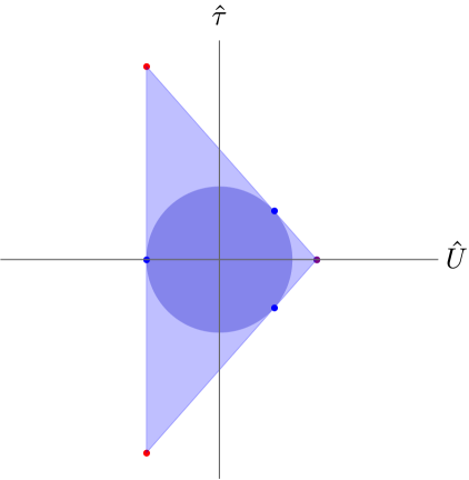
Figure 1: Convex hull condition for the species scale in M-theory on $T^{2}$ in the plane $(\hat{U},\hat{\tau})=(\frac{3}{\sqrt{14}}\log\mathcal{V}_{2}\,,\,\frac{1}{\sqrt{2}}\log\tau_{2})$. The blue dots in the facets represent the single KK towers, whereas the red and purple dots at the vertices represent string oscillator and double KK towers. The self-dual line $\hat{\tau}=0$ is fixed under the $\mathbb{Z}_{2}$-symmetry.

In order to check this, we proceed as in the 10d examples from sections 3.1 and 3.2. We look at the next non-trivial correction to the two-derivative lagrangian of maximal supergravity in 9d. Such operator happens to be precisely the one behaving schematically like $\mathcal{R}^{4}$, and it is still BPS protected. Its dependence with respect to the moduli space parametrised by $\{\mathcal{V}_{2},\tau\}$ has been already computed in [55, 37], and it is captured by the following function (see also [33])

$$S_{\mathcal{R}^{4}}^{\text{9d}}=\frac{1}{3\cdot 2^{8}\kappa_{9}^{2}}\int d^{9}x\sqrt{-g}\,\left(\frac{2\pi^{2}}{3}\mathcal{V}_{2}^{6/7}+\mathcal{V}_{2}^{-9/14}E_{3/2}^{sl_{2}}(\tau)\right)t_{8}t_{8}\mathcal{R}^{4}\,,$$ (3.24)

where $SL(2,\mathbb{Z})$ invariance in ensured by the non-holomorphic Eisenstein series of order $3/2$ (recall that the volume modulus is left unchanged under a modular transformation). The above operator has mass dimension $n=8$, such that according to eq. (3.8), we expect it to behave as $\mathcal{R}^{4}\Lambda_{\text{QG}}^{-6}$. We consider each asymptotic limit in Figure 1 in turn.

Let us start with the simplest ones. Thus, we will take the large/small radius limit while keeping $\tau$ fixed and finite. On the one hand, in the $\mathcal{V}_{2}\to\infty$ limit, the species scale coincides (up to order one factors) with the 11d Planck scale, which depends on the moduli fields as follows [19]

$$\frac{M_{\text{pl, 11}}}{M_{\text{pl, 9}}}\sim\left(\mathcal{V}_{2}\right)^{-1/7}\,.$$ (3.25)

Thus, we expect the the asymptotic behavior $\Lambda_{\text{QG}}^{-6}\sim\mathcal{V}_{2}^{6/7}$ in front of the quartic correction in (3.24), which is indeed the correct result.

In the opposite limit, namely when $\mathcal{V}_{2}\to 0$, the species counting is dominated by M2-branes wrapping the internal space. This actually corresponds to the KK tower implementing the M-theory/F-theory duality, such that the species scale becomes identical to the 10d (Type IIB) Planck scale, which reads [19]

$$\frac{M_{\text{pl, 10}}}{M_{\text{pl, 9}}}\sim\left(\mathcal{V}_{2}\right)^{3/28}\,.$$ (3.26)

Hence, according to (3.8), we expect the $\mathcal{R}^{4}$ to be controlled by $\Lambda_{\text{QG}}^{-6}\sim\left(\mathcal{V}_{2}\right)^{-9/14}$, and this indeed matches the behaviour observed in the second term in eq. (3.24), which of course dominates in the small volume limit.

Finally, let us check whether we can reproduce the expected dependence whenever the species scale is determined by the fundamental string mass, corresponding to the red dot in the upper half-plane in Figure 1, and whose tension may be readily computed [19]:

$$\frac{T_{\text{str}}}{M_{\text{pl, 9}}^{2}}\sim\left(\mathcal{V}_{2}\right)^{3/14}\,\left(\tau_{2}\right)^{-1/2}\,.$$ (3.27)

To do so, we consider two representative limits, namely $\tau_{2}\to\infty$ with $\mathcal{V}_{2}$ fixed and finite, and $\tau_{2}\sim\mathcal{V}_{2}^{-3}\to\infty$. In the former case, the species scale projects to $\Lambda_{\text{QG}}\sim\left(\tau_{2}\right)^{-1/4}$, such that $\Lambda_{\text{QG}}^{-6}\sim\left(\tau_{2}\right)^{3/2}$. This is exactly the asymptotic behaviour exhibited by the order-$3/2$ non-holomorphic Eisenstein series appearing in (3.24) (c.f. eq. (3.7) ). In the latter case, it is easy to see that the leading term in the correction is the second one in eq. (3.24), which behaves as $\mathcal{V}_{2}^{-9/14}\,\tau_{2}^{3/2}\sim m_{\text{str}}^{-6}$, where we have defined $m_{\text{str}}\equiv\sqrt{T_{\text{str}}}$, which is also in agreement with our prediction.

Several comments are now in order. First, as it was also the case for Type IIB String Theory in 10d, one would be tempted to propose $\Lambda_{\text{QG}}$ to be defined in the present nine-dimensional set-up precisely as

$$\Lambda_{\text{QG}}=\left(\frac{2\pi^{2}}{3}\mathcal{V}_{2}^{6/7}+\mathcal{V}_{2}^{-9/14}E_{3/2}^{sl_{2}}(\tau)\right)^{-1/6}\,,$$ (3.28)

which is automorphic and moreover reproduces the correct asymptotic behaviour in every infinite distance corner of the moduli space. However, let us stress one more time that this would imply, via eq. (3.8), that all the following higher order gravitational operators in the 9d effective action should also be accompanied by appropriate powers of the function (3.28), which is known not to be the case for e.g. higher curvature corrections involving derivatives of the quartic curvature invariants (see e.g., [33]). What seems to be true, though, is the fact that the species scale, as one typically defines it close to asymptotic boundaries in moduli space (see eq. (2.2)), is the energy scale controlling the EFT expansion of our quantum-gravitational theories, and thus should be taken as the true QG cut-off.

Second, notice that the function controlling the $t_{8}t_{8}\mathcal{R}^{4}$ term here is again an eigenfunction (with eigenvalue equal to $6/7$) of the Laplace operator in $SL(2,\mathbb{R})/SO(2)\times\mathbb{R}_{+}$

$$\Delta_{\text{9d}}=\Delta_{2}-\frac{7}{9}\,\mathcal{V}_{2}\,\partial_{\mathcal{V}_{2}}\left(\mathcal{V}_{2}\,\partial_{\mathcal{V}_{2}}\right)-\frac{1}{3}\,\mathcal{V}_{2}\,\partial_{\mathcal{V}_{2}}\,,$$ (3.29)

with $\Delta_{2}$ given in eq. (A.1) above. This was also the case in the 10d Type IIB case discussed before, and indeed the eigenvalue seems to be related to the power of the number of species that accompanies the operator under consideration.

Further tests

Porceeding as in the previous example, let us now look at the next few contributions to the four-(super)graviton effective action in 9d $\mathcal{N}=2$ supergravity. For the four-derivative term we have [33]

$$S_{\partial^{4}\mathcal{R}^{4}}^{\text{9d}}=\ell_{9}^{3}\int d^{9}x\sqrt{-g}\,\left(\frac{1}{2}\mathcal{V}_{2}^{-15/14}E_{5/2}^{sl_{2}}(\tau)+\frac{2\zeta(2)}{15}\mathcal{V}_{2}^{27/14}E_{3/2}^{sl_{2}}(\tau)+\frac{4\zeta(2)\zeta(3)}{15}\mathcal{V}_{2}^{-18/7}\right)\partial^{4}\mathcal{R}^{4}\,.$$ (3.30)

Notice that such term is also an eigenfunction of the scalar laplacian (3.29) with eigenvalue 30/7, as one may easily check. Moreover, the correction is compatible with the $SL(2,\mathbb{Z})$ invariance of the theory, such that we will restrict ourselves to the fundamental domain in what follows. The mass dimension of the operator is $n=12$, such that according to eq. (3.8) we expect an asymptotic dependence of the form $\Lambda_{\text{QG}}^{-10}\,\partial^{4}\mathcal{R}^{4}$ for (3.30) above. In particular, and as seen in the 10d type II examples studied above, this prediction is fulfilled in the cases in which we are probing an emergent string limit, namely when $\Lambda_{\text{QG}}=m_{s}$ , whereas in the decompactification limits one cannot direclty identify $\Lambda_{\text{QG}}^{-10}$ as the coefficient in front of this correction. Still, as argued before, this might be understood in terms of corrections which are not only sensitive to the purely quantum-gravitational effects associated with infinite towers of states becoming light asymptotically, whereas for the purely $\mathcal{R}^{4}$ this is the case and we believe it to be the relevant term in the expansion for the identification of the species scale.

3.4 M-theory on $T^{3}$

As our final example, let us consider maximal supergravity in eight spacetime dimensions, which arises upon compactifying e.g., Type IIB supergravity (c.f. eq. (3.1)) on a two-dimensional torus. Such process yields the following 8d action in the scalar-tensor sector [56]:

$$S_{\text{IIB}}^{\text{8d}}\,\supset \frac{1}{2\kappa_{8}^{2}}\int d^{8}x\sqrt{-g}\left[\mathcal{R}-\frac{1}{6}\frac{(\partial\nu)^{2}}{\nu^{2}}-\frac{\partial\tau\cdot\partial\bar{\tau}}{2\tau_{2}^{2}}-\frac{\partial U\cdot\partial\bar{U}}{2U_{2}^{2}}-\nu\frac{\left|\tau\partial b+\partial c\right|^{2}}{2\tau_{2}}\right]\,,$$ (3.31)

where $U$ denotes the complex structure of the internal torus, $\nu=\left(\tau_{2}\mathcal{V}_{2}^{2}\right)^{-1}$ is an $SL(2,\mathbb{Z})_{\tau}\,$-invariant volume, and $b,c$ are scalar fields arising from the reduction of the NS and RR 2-form fields of 10d $\mathcal{N}=(2,0)$ supergravity on the internal 2-cycle. Note that there are two modular symmetries visible from the action (3.31) above: that associated to the axio-dilaton, which is inherited from ten dimensions, as well as an additional one which transforms the complex $U$ field in a fractional linear fashion. There is, however, an extra ‘hidden’ $SL(2,\mathbb{Z})_{T}$ symmetry associated to the Kähler modulus $T=b+i\mathcal{V}_{2}$, which can be made manifest upon changing variables from $\{\nu,\tau\}\leftrightarrow\{\varphi_{8},T\}$, where $\varphi_{8}$ denotes the 8d dilaton (c.f. eq. (B.6))

$$e^{-2\varphi_{8}}=e^{-2\phi}\mathcal{V}_{2}\,.$$ (3.32)

What is important for us is that the full U-duality symmetry of the theory is actually larger, namely it consists of $SL(2,\mathbb{Z})\times SL(3,\mathbb{Z})$, where the modular factor acts solely on the complex structure modulus. In fact, upon introducing the following symmetric $3\times 3$ matrix with unit determinant [56]

$$\mathcal{B}=\nu^{1/3}\begin{pmatrix}\frac{1}{\tau_{2}}\quad\frac{\tau_{1}}{\tau_{2}}\quad\frac{c+\tau_{1}b}{\tau_{2}}\\ \frac{\tau_{1}}{\tau_{2}}\quad\frac{|\tau|^{2}}{\tau_{2}}\quad\frac{\tau_{1}c+|\tau|^{2}b}{\tau_{2}}\\ \frac{c+\tau_{1}b}{\tau_{2}}\quad\frac{\tau_{1}c+|\tau|^{2}b}{\tau_{2}}\quad\frac{1}{\nu}+\frac{|c+\tau b|^{2}}{\tau_{2}}\end{pmatrix}\,,$$ (3.33)

which transforms (c.f. eq. (A.11)) in the adjoint representation of $SL(3,\mathbb{Z})$, one can rewrite the above action in a manifestly $SL(2,\mathbb{Z})\times SL(3,\mathbb{Z})$ invariant way

$$S_{\text{IIB}}^{\text{8d}}\,\supset \frac{1}{2\kappa_{8}^{2}}\int d^{8}x\sqrt{-g}\left[\mathcal{R}-\frac{\partial U\cdot\partial\bar{U}}{2U_{2}^{2}}+\frac{1}{4}\text{tr}\left(\partial\mathcal{B}\cdot\partial\mathcal{B}^{-1}\right)\right]\,,$$ (3.34)

Therefore, we conclude that the moduli space of the theory is described by a coset of the form $\mathcal{M}_{\text{8d}}=SL(2,\mathbb{Z})\backslash SL(2,\mathbb{R})/U(1)\times SL(3,\mathbb{Z})\backslash SL(3,\mathbb{R})/SO(3)$, where the discrete piece corresponds to the U-duality group of the eight-dimensional theory [50].

In the following, it will be useful to phrase the present discussion using a dual description in terms of M-theory compactified on a three-torus, whose bosonic action reads [58]

$$S_{\text{M-th}}^{\text{8d}}\,\supset\, \frac{1}{2\kappa_{8}^{2}}\int d^{8}x\,\sqrt{-g}\,\left[\mathcal{R}-\frac{1}{4}\left(g^{ii^{\prime}}g^{jj^{\prime}}+\frac{1}{6}g^{ij}g^{i^{\prime}j^{\prime}}\right)\partial g_{ij}\partial g_{i^{\prime}j^{\prime}}-\frac{1}{2\mathcal{V}_{3}^{2}}\left(\partial C^{(3)}_{123}\right)^{2}\right]\,,$$ (3.35)

where $g_{ij}$ is the internal metric, $\mathcal{V}_{3}$ its overall volume in M-theory units and the scalar $C^{(3)}_{123}$ arises by reducing the antisymmetric 3-form field along the $T^{3}$. In order to make contact with the previous Type IIB perspective, one needs to identify the modulus $U$ with a complex field $\mathcal{T}$, which is defined as follows

$$\mathcal{T}=C^{(3)}_{123}+\text{i}\mathcal{V}_{3}\,,$$ (3.36)

as well as relate the fields captured by the matrix $\mathcal{B}$ in eq. (3.33) with the ‘unimodular’ metric components of the torus, namely $\mathcal{B}_{ij}\rightarrow\tilde{g}_{ij}=\mathcal{V}_{3}^{-1/3}g_{ij}$. This indeed recovers the action (3.34) written in a manifestly $SL(3,\mathbb{Z})$ invariant way, as explained in Appendix B.

Once again, one would expect the species scale $\Lambda_{\text{QG}}$ to be an automorphic function of the moduli, whose asymptotic behaviour should match that predicted by [19, 25]. This is summarised in Figure 2 below, where the convex hull generated by the relevant $\mathcal{Z}$-vectors is explicitly shown.

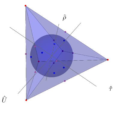
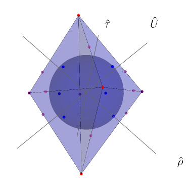
Figure 2: Convex hull for the species scale in M-theory on $T^{3}$ with the axions set to a constant value from two different angles. The blue dots in the facets of the convex hull correspond to single KK towers ($n=1$), the light purple dots in the edges indicate double KK towers ($n=2$) and the purple and red dots in the vertices correspond to triple KK towers ($n=3$) and string towers, respectively.

Before proceeding further with a systematic study of the higher-dimensional operators appearing in the 8d effective action and their relation to the QG cut-off, let us first try to guess what could be the $SL(2,\mathbb{Z})$ dependence of the species scale based on our general discussion in Section 2.2. In the general discussion around eq. (2.18), we saw how the parameter $\gamma$ in eq. (2.6) should depend on the spacetime dimension of our theory in order to match the familiar (asymptotic) decay rate for the species scale, as well as on the nature of the infinite distance points that are present. This raises then the following natural question: What happens when the modular parameter, $\tau$, is rather associated with some decompactification process? In such a case, the tower becoming light the fastest at the infinite distance point $\tau\to\text{i}\infty$ is of Kaluza-Klein nature. An example of this is given precisely by M-theory on $T^{3}$, where the modular parameter is the complex field $\mathcal{T}$ defined in eq. (3.36).

Therefore, upon applying eqs. (2.17) and (2.18) to the present eight-dimensional example in the limit $\mathcal{T}\to\text{i}\infty$ (which essentially decompactifies the 8d theory back to the original 11d supergravity) we obtain $\gamma=1$, leading to the following functional form for a subset of the total number of light species

$$N\supset\left[-\text{log}\left(\mathcal{T}_{2}\,|\eta(\mathcal{T})|^{4}\right)\right]\sim\mathcal{T}_{2}\,,\qquad\text{as}\qquad\mathcal{T}_{2}\to\infty\,.$$ (3.37)

The $\mathcal{R}^{4}$ operator

In order to check the proposed species function (3.37), as well as to further extend it so as to include the additional $SL(3,\mathbb{R})/SO(3)$-sector, one can look at known higher-dimensional operators appearing in the 8d $\mathcal{N}=2$ effective action. Therefore, we start from the general form for the scalar and gravitational sector of the theory

$$\mathcal{L}^{8d}_{\mathcal{R}^{4}}\supset\frac{1}{2\kappa_{8}^{2}}\left[\left(\mathcal{R}+\sum_{k}\frac{\mathcal{O}_{k}(\mathcal{R})}{\Lambda_{\text{QG}}^{k-2}}\right)-\frac{\partial\mathcal{T}\cdot\partial\bar{\mathcal{T}}}{2\mathcal{T}_{2}^{2}}\right]\ ,$$ (3.38)

A particularly interesting operator in this regard within a given spacetime dimension $d$ is that verifying $k=d$, since eqs. (2.2) and (3.38) predict an asymptotic moduli dependence for it of the form $\Lambda_{\text{QG}}^{2-d}\,\mathcal{O}_{d}(\mathcal{R})\sim N_{\text{sp}}(T)\,\mathcal{O}_{d}(\mathcal{R})$. Incidentally, in the 4d $mathcal{N}=2$ case analyzed in the following subsection, this is precisely the coefficient of the operator $\mathcal{R}^{2}$, which is controlled by the topological genus one partition function $\mathcal{F}_{1}$ for $\mathcal{N}=2$ theories. In our 8d set-up, it would rather correspond to a term behaving schematically like $\mathcal{R}^{4}$. This was already computed and studied in detail in [37, 49], and it reads as follows

$$\mathcal{L}^{8d}_{\mathcal{R}^{4}}=\frac{1}{2\kappa_{8}^{2}}\left(\hat{E}_{3/2}^{sl_{3}}+2\hat{E}_{1}^{sl_{2}}\right)\,t_{8}t_{8}\mathcal{R}^{4}\ ,$$ (3.39)

where $\hat{E}_{1}^{sl_{2}},\hat{E}_{3/2}^{sl_{3}}$ are the (regularised) Eisenstein series of order 1 and 3/2 for $SL(2,\mathbb{Z})$ and $SL(3,\mathbb{Z})$, respectively (see Appendix A). In the following, we show that the expression (3.39) matches asymptotically the diagram depicted in Figure 2. First, notice that due to $SL(2,\mathbb{Z})\times SL(3,\mathbb{Z})$ duality, it is enough to focus on a fundamental domain, since it contains the minimal non-redundant information captured by the convex hull diagram [19, 59]. For concreteness we take the sub-polytope generated by the vertices corresponding to a fundamental Type II string, a 10d Planck scale implementing M/F-theory duality and the 11d Planck mass of the full decompactified theory. These vectors read [19]:

$$\begin{split}\vec{\mathcal{Z}}_{\text{osc},\,3}&=\left(0,-\sqrt{\frac{2}{21}},\frac{1}{\sqrt{14}}\right)\,,\qquad\vec{\mathcal{Z}}_{\text{KK-M},\,3}=\left(\frac{1}{4\sqrt{2}},-\frac{1}{2\sqrt{42}},\frac{1}{4\sqrt{14}}\right)\,,\\ \vec{\mathcal{Z}}_{\text{KK},\,(123)}&=\left(0,\frac{1}{\sqrt{42}},\frac{2}{3\sqrt{14}}\right)\,,\end{split}$$ (3.40)

where the notation follows that of ref. [19], namely $\vec{\mathcal{Z}}=\left(\mathcal{Z}^{\hat{\tau}},\mathcal{Z}^{\hat{\rho}},\mathcal{Z}^{\hat{U}}\right)$. In terms of the M-theory variables $\{\tau_{2},R_{3},\mathcal{V}_{2}\}$ (see eq. (B.3)), one finds three relevant (asymptotic) QG cut-offs (in 8d Planck units):

$$\begin{split}m_{\text{str},\,3}&\sim R_{3}^{1/3}\,\mathcal{V}_{2}^{-3/14}\,,\qquad M_{\text{pl},\,10}\sim R_{3}^{1/12}\,\mathcal{V}_{2}^{-3/56}\,\tau_{2}^{-1/8}\,,\\ M_{\text{pl},\,11}&\sim R_{3}^{-1/6}\,\mathcal{V}_{2}^{-1/7}\sim\mathcal{V}_{3}^{-1/6}\,,\end{split}$$ (3.41)

which eq. (3.39) ought to reproduce upon taking appropriate limits. These correspond to the mass scale of a fundamental Type II string, as well as the 10d and 11d Planck masses of dual F-/M-theory descriptions.

For simplicity, we first consider the $T^{3}$ decompactification limit $\mathcal{V}_{3}\to\infty$, where $\Lambda_{\text{QG}}=M_{\text{pl},\,11}$ asymptotically. This is associated to the $SL(2,\mathbb{Z})$ sector of the theory, since from eq. (A.8) it follows that

$$2\hat{E}_{1}^{sl_{2}}(\mathcal{T})=-2\pi\text{log}\left(\mathcal{T}_{2}\,|\eta(\mathcal{T})|^{4}\right)\,\sim\,\frac{\pi^{2}}{3}\mathcal{V}_{3}\,\propto\,\left(\frac{M_{\text{pl, 8}}}{M_{\text{pl, 11}}}\right)^{6}\,,$$ (3.42)

where the asymptotic dependence should be understood when taking the limit $\mathcal{T}_{2}\to\infty$. This matches exactly with our prediction in eq. (3.37) above for the $SL(2,\mathbb{Z})$ sector.

Now, in order to see how the remaining two scales in eq. (3.41) are recovered from (3.39), we will need to take appropriate asymptotic limits of the order-3/2 Eisenstein series $\hat{E}_{3/2}^{sl_{3}}$. Indeed, upon using the expansion (A.2), one finds (at leading order)

$$\hat{E}_{\ell}^{sl_{3}}\,\sim\,2\zeta(3)\mathcal{V}_{2}^{9/7}\,R_{3}^{-2}\,\propto\,\left(\frac{m_{\text{str},\,3}}{M_{\text{pl},\,8}}\right)^{-6}\,,$$ (3.43)

where we have mapped $\nu\to\mathcal{V}_{2}^{-9/14}\,R_{3}\,\tau_{2}^{-3/2}$ upon performing Type IIB/M-theory duality in 8d (see discussion around eq. (B.19)). This in turn reproduces (any of) the red dot(s) in Figure 2.

Finally, to see how the 10d F-theory (or rather Type IIB) Planck scale arises within $\hat{E}_{\ell}^{sl_{3}}$, one can take a limit where $\mathcal{V}_{2}^{-9/14}\,R_{3}\,\tau_{2}^{-3/2}\to\infty$ with $\mathcal{V}_{2}^{9/14}\,R_{3}^{-1}\,\tau_{2}^{-1/2}$ kept fixed. In the dual Type IIB frame, this corresponds to taking $\nu\to\infty$ with $\tau_{2}$ fixed to a constant value (see Appendix B for details on this point). Along such limit, $\hat{E}_{\ell}^{sl_{3}}$ behaves asymptotically like $\nu^{-1/2}$, which indeed coincides with $M_{\text{pl},\,10}^{-6}$ in 8d Planck units (c.f. eq. (3.41)).

All in all, we conclude that the function $N_{\text{sp}}=\hat{E}_{3/2}^{sl_{3}}+2\hat{E}_{1}^{sl_{2}}$ seems to capture all relevant asymptotic behaviours of the spacies scale in 8d maximal supergravity, being moreover invariant under the $SL(2,\mathbb{Z})\times SL(3,\mathbb{Z})$ U-duality group and thus reproducing precisely the convex hull diagram depicted in Figure 2.

Finally, as for the previous cases, other corrections proportional to extra derivatives of the quartic curvature invariants that have been computed in the literature [33] are not suppressed by the corresponding power of the species scale, but by some more intrincate combinations of scales. As discussed above, we expect this to be the case in general, but we believe the $\mathcal{R}^{4}$ correction is the one capturing the UV divergence of the EFT that should be related to the species scale.

3.5 4d $\mathcal{N}=2$ theories

The analysis around eq. (2.18) can be used to predict as well the value of $\gamma$ for emergent string/decompactification limits occurring in 4d theories exhibiting some sort of modular invariance. These models have been thoroughly studied (and were the original arena for the proposal of a globally defined species scale in [24]). Particularly relevant for our proposal are those which descend from e.g., heterotic compactifications on $K3\times T^{2}$ (or obifolded versions thereof, see e.g. [60]). Within such $\mathcal{N}=2$ models, one finds for the one-loop contribution to the holomorphic gauge kinetic function the following functional dependence

$$f_{a}\ =\ S\ -\ \frac{1}{16\pi^{2}}\sum_{i=1}^{3}\ b_{a,i}^{\mathcal{N}=2}\ \text{log}\left(\text{Im}\,T_{i}|\eta(T_{i})|^{4}\,\text{Im}\,U_{i}|\eta(U_{i})|^{4}\right)\ ,$$ (3.44)

where the tree level piece is given by the (complexified) 4d dilaton $S$, whilst the loop correction depends both on the Kähler and complex structure moduli associated to the torus. This latter piece incorporates the sum over towers of KK and winding states whose mass depends on $T_{i}$ and $U_{i}$.

Let us take the simplest possible example, namely we consider Type IIA compactified on the Enriques CY $\left(K3\times T^{2}\right)/\mathbb{Z}_{2}$, which is dual to a heterotic compactification on $K3\times T^{2}$. In this case, one finds (at large volume) that the moduli space metric behaves as $G_{T\bar{T}}=\frac{1}{4T_{2}^{2}}\,$, whereas the genus-one topological free energy, which controls the $R^{2}$ term in the gravitational EFT, takes the following form [25, 38]

$$\mathcal{F}_{1}=-6\log\left(T_{2}|\eta(T)|^{4}\right)+\beta\,.$$ (3.45)

Hence, according to our Ansatz (2.6), we predict for the present 4d set-up a value $\gamma=1$, which is precisely what is observed in eq. (3.45) above.

An analysis along similar lines can be performed when probing other kind of limits within the vector multiplet sector of 4d $\mathcal{N}=2$ theories, including partial decompactifications to M-/F-theory in 5 and 6 spacetime dimensions, respectively. This was done in detail in refs. [24, 25], so we refrain from repeating it here and refer the interested reader to the original references.

4 Summary and Discussion

In the present work we have pursued the idea of trying to identify the species scale as the energy cut-off signalling the breakdown of a semi-classical description of gravity, as originally proposed in [10, 11]. The main focus has been placed on looking at the moduli dependence of certain higher-dimensional operators in the EFT expansion, following the ideas in [24, 25]. Such terms seem to probe the ultra-violet nature of Quantum Gravity in a non-trivial way, and indeed can have a great impact on the IR physics through e.g., (small) Black Holes and entropy considerations (see e.g. [28, 20]).

We thus first described what are the expectations from a purely EFT analysis in Section 2.1, where naively one could think that the higher-dimensional operators coming from higher curvature invariants are suppressed with respect to the Einstein-Hilbert term — with appropriate powers of the UV cut-off. Next, in Section 2.2 and based on duality symmetry considerations, we proposed an strategy to look for potential candidates for a globally-defined species scale function in certain instances (see also [30] for related ideas). We exemplified such considerations within the particular case of $SL(2,\mathbb{Z})$, which arises in many instances in String Theory and where the mathematical theory of modular functions is fully developed, such that it can be readily applied. However, we noticed that the minimal requirements for a bona-fide species scale, namely the fact that it should be bounded from above (by the Planck scale) and that it should go to zero asymptotically, are not strong enough so as to uniquely determine such functions. These can be given in general by combinations of ‘well-behaved’ automorphic forms (see Appendix A), such that there is no fundamental reason a priori to select any particular one. Despite this apparent freedom, and based on our String Theory experience as well as certain threshold computations existing in the literature [61], we proposed a certain (regularised) non-holomorphic Eisenstein function as a proxy for the species scale in any $SL(2,\mathbb{Z})$-sector of the theory.

Later on, we tested these ideas in simple and well-understood highly supersymmetric set-ups. In particular, we analysed the structure of the first higher-dimensional/derivative (BPS-protected) operators in maximal supergravity in 10, 9 and 8 dimensions. There, the first non-trivial correction to the two-derivative lagrangian, which is completely fixed by supersymmetry, arises from certain combinations of four Riemann tensors (see Section 3). In all these cases, the moduli-dependent function controlling such terms in the EFT was seen to match asymptotically with the usual species counting computations [17, 19] in a non-trivial fashion. This means that, starting from any dual frame, one can retrieve the fundamental QG scale of any other corner of the duality web of the theory, including those living in higher dimensions. This extends the results from refs. [24, 25], where a similar procedure was performed in 4d theories with eight supercharges. Despite this agreement with our expectations from Section 2.1, several relevant observations were made. First, the simple expansion in power series of the inverse cut-off was seen to arise only asymptotically. Therefore, even though when expanding around any infinite distance corner of the moduli space the different gravitational operators are suppressed by the appropriate species scale, this may be no longer the case when venturing towards the bulk. We believe this has to do with the fact that the expansion in (2.1) should be taken as some sort of approximation strictly valid close to the infinite distance boundaries, where weak couplings appear and the perturbative series rapidly converge. There, the classical dimension of the different operators in the EFT expansion is a good proxy, whilst at the interior, large quantum corrections (perturbative and non-perturbative) may occur, thus giving rise to big ‘anomalous dimensions’. Second, we found that certain non-leading gravitational operators in the theory, given by higher derivatives of four Riemann tensors contracted in some specific way [32, 33], do not seem to exactly follow the pattern proposed in eq. (2.1), but are instead controlled by different integer powers of the lightest tower scale (rather than the species scale). This was interpreted as pointing out that such operators are not really sensitive to the UV cut-off of the theory, but instead are generated by integrating out the towers in a UV-convergent way. Therefore, it seems reasonable that the right way to proceed in order to properly identify the species scale in a given theory is to look at the low-dimensional (but no present in the two-derivative action) relevant or marginal operators, which really probe the UV-physics of the theory.

Another interesting feature that we observed was that these operators present a particular moduli dependence tightly related to the moduli space geometry. Indeed, the functional coefficients were seen to satisfy certain eigenvalue/Poisson equations with respect to the moduli space laplacian. In some cases, these can be related to supersymmetry (see e.g., [62] and references therein), but it is not entirely clear if it is really a consequence of the latter, of rather some deep property of the species scale. In particular, it would be interesting to investigate whether the presence of this eigenvalue/Poisson equation could be related to certain IR swampland conditions, such as the SWGC [63] (see also [64, 65]). We leave further investigation of these issues for future work.

Finally, several questions can be raised at this point. First of all, the role of the species scale in the gravitational EFT expansion might not be fully understood yet. It would be interesting to pinpoint precisely which operators can be expected to be suppressed by the appropriate powers of the species scale (instead of just that of the towers). One could also try to extend these analysis to other set-ups both in different number of spacetime dimensions and supersymmetries. This is particularly interesting in the case of 16 supercharges or less, where certain infinite distance limits probe running-solutions (i.e., not vacua) [66] and where the computation of the species scale seems challenging [59]. Finally, one could try to study further implications of these considerations within the Swampland Program, as well as to revisit certain naturalness/fine tuning arguments that are commonly employed in model building scenarios.

Acknowledgments

We would like to thank F. Marchesano, M. Montero, D. Prieto, I. Ruiz, A. Uranga, I. Valenzuela for useful discussions and correspondence. A.C. would like to thank the Theoretical Physics Department at CERN for hospitality and support, where most of the work was completed. This work is supported through the grants CEX2020-001007-S and PID2021-123017NB-I00, funded by MCIN/AEI/10.13039/501100011033 and by ERDF A way of making Europe. The work of A.C. is supported by the Spanish FPI grant No. PRE2019-089790 and by the Spanish Science and Innovation Ministry through a grant for postgraduate students in the Residencia de Estudiantes del CSIC.

Appendix A Relevant Automorphic Forms

This appendix serves as a mathematical compendium for the relevant set of automorphic functions that appear at several instances in the discussion from the main text. We will focus mostly on the discrete groups $SL(2,\mathbb{Z})$ and $SL(3,\mathbb{Z})$, since they capture the duality symmetries in 10, 9 and 8d maximal supergravity (see Section 3). A similar analysis can be performed for the (bigger) duality groups that arise upon descending in the number of non-compact spacetime dimensions, but we refrain from reviewing those in the present work (see [32] for details).

A.1 $SL(2,\mathbb{Z})$ Maas waveforms

An automorphic function of a given (Lie) group $G$ is defined as a map from a given space $\mathcal{M}$, which admits some natural action group action for $G$, to $\mathbb{R}$ (or more generally $\mathbb{C}$), such that is left invariant under the corresponding group action for any $g\in G$. In the following, we will particularise to those automorphic functions of $SL(2,\mathbb{Z})$ which are moreover real analytic, since those may appear as (generalised) ‘Wilson coefficients’ in the EFT expansion of our gravitational effective field theories. In fact, there is an economic way to generate such analytic functions as eigenfunctions of some appropriate elliptic operator previously defined. Now, since we want these functions to be automorphic forms as well, we can simply take the hyperbolic Laplace operator, which is both elliptic and $SL(2,\mathbb{Z})$-invariant (in a precise sense that we specify below). This operator reads

$$\Delta_{2}=\tau_{2}^{2}\left(\frac{\partial^{2}}{\partial\tau_{1}^{2}}+\frac{\partial^{2}}{\partial\tau_{2}^{2}}\right)\,,$$ (A.1)

where again we define $\tau=\tau_{1}+\text{i}\tau_{2}$. Note that this is nothing but the Laplacian operator associated to the metric (2.4). Therefore, the eigenfunctions of this operator — which are moreover modular invariant — are called singular Maas forms [62]. Here we will be interested, for reasons that will become clear later on, in a subgroup of such set of functions, those denoted simply as Maas forms, which have the additional property of growing polynomially (instead of exponentially) with $\tau_{2}$, as $\tau_{2}\to\infty$. An example of Maas form that will play a key role in the following are the so-called non-holomorphic Eisenstein series [62]

$$\frac{\Gamma(\ell)}{2\pi^{\ell}}\,E_{\ell}^{sl_{2}}(\tau)\equiv\pi^{-\ell}\,\Gamma(\ell)\,\frac{1}{2}\sum_{(m,n)\in\mathbb{Z}^{2}\setminus\{(0,0)\}}\frac{\tau_{2}^{\ell}}{\left|m+n\tau\right|^{2\ell}}\,,$$ (A.2)

which converge absolutely if $\text{Re}\,\ell>1$. It can be shown (upon using that the fractional linear transformation in eq. (2.5) conmutes with the operator $\Delta_{2}$), that indeed $E_{\ell}^{sl_{2}}(\tau)$ are both automorphic and eigenfunctions of the hyperbolic Laplacian, with eigenvalue given by $\ell(\ell-1)$. The polynomial growth of the Eisenstein series can be also easily understood, since upon taking the limit $\tau_{2}\to\infty$, the infinite series is clearly dominated by the terms with $n=0$, which grows as $\tau_{2}^{\ell}$. More precisely, the functions $E_{\ell}^{sl_{2}}(\tau)$ have an alternative Fourier expansion in $\tau_{1}$, which can be obtained upon Poisson resumming on the integer $n$, yielding

$$E_{\ell}^{sl_{2}}=\, \bigg{[}2\zeta(2\ell)\tau_{2}^{\ell}+2\pi^{1/2}\frac{\Gamma(\ell-1/2)}{\Gamma(\ell)}\zeta(2\ell-1)\tau_{2}^{1-\ell}$$

$$+\frac{8\pi^{\ell}\tau_{2}^{1/2}}{\Gamma(\ell)}\sum_{m=1}^{\infty}m^{\ell-1/2}\sigma_{1-2\ell}(m)\,\cos(2\pi m\tau_{1})\,K_{\ell-1/2}(2\pi m\tau_{2})\bigg{]}\,,$$ (A.3)

where $\sigma_{1-2\ell}(m)=\sum_{d|m}d^{\ell}$ runs over all divisors $d$ of $m$, and $K_{\ell}(y)$ is the modified Bessel function of second kind, which is defined as follows

$$K_{\ell}(y)=\frac{1}{2}\int_{0}^{\infty}dx\,x^{\ell-1}\exp\left[-\frac{y}{2}\left(x+\frac{1}{x}\right)\right]\,,$$ (A.4)

and decays asymptotically as $K_{\ell}(y)\sim\sqrt{\frac{\pi}{2y}}e^{-y}$ for $y\to\infty$.

Let us finally mention that the modular function $\left(2\pi^{\ell}\right)^{-1}\Gamma(\ell)E_{\ell}^{sl_{2}}(\tau)$, when seen as a function also of the variable $\ell$, has a meromorphic continuation to al $\ell\in\mathbb{C}$, which is thus analytic everywhere except for simple poles at $\ell=0,1$. Moreover, if the divergence for $\ell=1$ is ‘extracted’, namely upon selecting the constant term (with respect to $\ell$) in the Laurent series for $E_{\ell}^{sl_{2}}$ at $\ell=1$, one obtains the following function [62]

$$2\pi\left(\gamma_{\text{e}}-\log 2\right)-\pi\log\left(\tau_{2}\,|\eta(\tau)|^{4}\right)\,,$$ (A.5)

where $\gamma_{\text{e}}$ is the Euler-Mascheroni constant and $\eta(\tau)$ denotes the Dedekind eta function, which may be defined as follows

$$\eta(\tau)=q^{\frac{1}{24}}\prod_{k=1}^{\infty}\left(1-q^{k}\right)\,,\qquad q=e^{2\pi i\tau}\,.$$ (A.6)

To conclude, let us note that even though the function $\hat{E}_{1}^{sl_{2}}(\tau)=-\pi\log\left(\tau_{2}\,|\eta(\tau)|^{4}\right)$ arises as some sort of analytic extension of $E_{1}^{sl_{2}}(\tau)$, it is actually not a Maas form, since $\Delta_{2}\hat{E}_{1}^{sl_{2}}(\tau)$ is not proportional to $\hat{E}_{1}^{sl_{2}}(\tau)$ itself but it rather gives a constant value. This can be easily checked upon noting that $\partial\bar{\partial}\hat{E}_{1}^{sl_{2}}(\tau)=\frac{\pi}{4\tau^{2}_{2}}$, as well as $\Delta_{2}=4\tau_{2}^{2}\partial\bar{\partial}$, where we have defined $\partial=\partial/\partial\tau$ and $\bar{\partial}=\partial/\partial\bar{\tau}$. In any event, what remains true is that the large modulus behaviour of $\hat{E}_{1}^{sl_{2}}(\tau)$ matches with that expected for $E_{\ell=1}^{sl_{2}}(\tau)$, since upon using the Fourier series expansion for $\eta(\tau)$

$$\eta(\tau)=q^{\frac{1}{24}}\left(1-q-q^{2}+q^{5}+\mathcal{O}(q^{7})\right)\,,$$ (A.7)

one finds the following relevant asymptotic expression

$$-\pi\text{log}\left(\tau_{2}\,|\eta(\tau)|^{4}\right)\,\sim\,-\pi\text{log}\left(\tau_{2}\,e^{-\frac{\pi\tau_{2}}{3}}\right)\,\sim\,\frac{\pi^{2}}{3}\tau_{2}-\pi\text{log}(\tau_{2})\,,$$ (A.8)

whose first term precisely is $2\zeta(2)\tau_{2}$ (c.f. eq. (A.1)).

A.2 $SL(3,\mathbb{Z})$ Maas waveforms

With an eye to future applications within maximal supergravity in $d=8$ spacetime dimensions, let us extend the previous analysis so as to incorporate other groups into the game. Such groups typically appear as the U-dualities of the corresponding supergravity theory, a prototypical example being $SL(3,\mathbb{Z})$ (see e.g., [58]). The question then is: Can we analogously define automorphic forms for $SL(3,\mathbb{Z})$ following the same procedure as for the Möbius group? The answer turns out to be yes, as we outline below.

Therefore, let us first introduce the appropriate elliptic $SL(3,\mathbb{Z})$-invariant operator, namely the Laplace operator on the coset space $SL(3,\mathbb{R})/SO(3)$

$$\Delta_{3}=4\tau_{2}^{2}\partial_{\tau}\partial_{\bar{\tau}}+\frac{1}{\nu\tau_{2}}\left|\partial_{b}-\tau\partial_{c}\right|^{2}+3\partial_{\nu}\left(\nu^{2}\partial_{\nu}\right)\,,$$ (A.9)

where the precise (physical) meaning of the different coordinates will become clear later on in Section 3.4. For the time being, it is enough to realise that the previous coordinates can be compactly grouped into the following $3\times 3$ matrix (see e.g., [57])

$$\mathcal{B}=\nu^{1/3}\begin{pmatrix}\frac{1}{\tau_{2}}\quad\frac{\tau_{1}}{\tau_{2}}\quad\frac{c+\tau_{1}b}{\tau_{2}}\\ \frac{\tau_{1}}{\tau_{2}}\quad\frac{|\tau|^{2}}{\tau_{2}}\quad\frac{\tau_{1}c+|\tau|^{2}b}{\tau_{2}}\\ \frac{c+\tau_{1}b}{\tau_{2}}\quad\frac{\tau_{1}c+|\tau|^{2}b}{\tau_{2}}\quad\frac{1}{\nu}+\frac{|c+\tau b|^{2}}{\tau_{2}}\end{pmatrix}\,,$$ (A.10)

which moreover satisfies $\mathcal{B}=\mathcal{B}^{\text{T}}$ as well as $\det\mathcal{B}=1$. The reason why it is useful to introduce the matrix $\mathcal{B}$ is because it transforms in the adjoint representation of $SL(3,\mathbb{Z})$, namely upon performing some transformation $\mathcal{A}\in SL(3,\mathbb{Z})$, one finds that

$$\mathcal{B}\rightarrow\mathcal{A}^{\text{T}}\,\mathcal{B}\,\mathcal{A}\,.$$ (A.11)

With this, we are now ready to define the Eisenstein $SL(3,\mathbb{Z})$ series of order $\ell$:

$$E_{\ell}^{sl_{3}}=\sum_{\mathbf{n}\,\in\,\mathbb{Z}^{3}\setminus\{\vec{0}\}}\left(\sum_{i,j=1}^{3}n_{i}\,\mathcal{B}^{ij}\,n_{j}\right)^{-\ell}=\sum_{\mathbf{n}\,\in\,\mathbb{Z}^{3}\setminus\{\vec{0}\}}\nu^{-\ell/3}\left[\frac{\left|n_{1}+n_{2}\tau+n_{3}\left(c+\tau b\right)\right|^{2}}{\tau_{2}}+\frac{n_{3}^{2}}{\nu}\right]^{-\ell}\,,$$ (A.12)

with $\mathcal{B}^{ij}$ denoting the components of the inverse matrix of $\mathcal{B}$. Note that the above expression is manifestly $SL(3,\mathbb{Z})$-invariant, since the vector $\textbf{n}=\left(n_{1},n_{2},n_{3}\right)$ transforms as $\textbf{n}\rightarrow\mathcal{A}^{\text{T}}\,\textbf{n}$ under the duality group. As also happened with the non-holomorphic Eisenstein series defined in eq. (A.2) above, the functions $E_{\ell}^{sl_{3}}$ are eigenvectors of the Laplacian $\Delta_{3}$, satisfying

$$\Delta_{3}E_{\ell}^{sl_{3}}=\frac{2\ell(2\ell-3)}{3}E_{\ell}^{sl_{3}}\,.$$ (A.13)

Let us also mention that the series $E_{\ell}^{sl_{3}}$, when viewed as a function of $\ell$, are absolutely convergent for $\ell>3/2$, whilst $E_{3/2}^{sl_{3}}$ is logarithmically divergent. This state of affairs reminds us of the situation for the modular non-holomorphic Eisenstein series $E_{\ell}^{sl_{2}}$, which had a simple pole for $\ell=1$. Therefore, proceeding analogously as in that case, one may define

$$\hat{E}_{3/2}^{sl_{3}}\equiv\lim_{\ell\to 3/2}\left(E_{\ell}^{sl_{3}}-\frac{2\pi}{\ell-3/2}-4\pi(\gamma_{\text{e}}-1)\right)\,,$$ (A.14)

where again $\gamma_{\text{e}}$ denotes the Euler-Mascheroni constant. Such newly defined function is no longer singular and remains invariant under $SL(3,\mathbb{Z})$ transformations, with the price of not being a zero-mode of the Laplacian (A.9) anymore.

Fourier-like expansions

In what follows we will try to rewrite the $SL(3,\mathbb{Z})$ Eisenstein series in a way which makes manifest the perturbative and non-perturbative origin of the different terms that appear in the expansion, similarly to what we did for the $SL(2,\mathbb{Z})$ case. We closely follow Appendix A of [57]. First, let us introduce the following integral representation

$$E_{\ell}^{sl_{3}} =\frac{\pi^{\ell}}{\Gamma(\ell)}\int_{0}^{\infty}\frac{dx}{x^{1+\ell}}\sum_{\mathbf{n}\,\in\,\mathbb{Z}^{3}\setminus\{\vec{0}\}}\exp\left[-\frac{\pi}{x}\left(\sum_{i,j=1}^{3}n_{i}\,\mathcal{B}^{ij}\,n_{j}\right)\right]$$

$$=\nu^{-\ell/3}\frac{\pi^{\ell}}{\Gamma(\ell)}\int_{0}^{\infty}\frac{dx}{x^{1+\ell}}\sum_{\mathbf{n}\,\in\,\mathbb{Z}^{3}\setminus\{\vec{0}\}}\exp\left[-\frac{\pi}{x}\left(\frac{\left|n_{1}+n_{2}\tau+n_{3}\left(c+\tau b\right)\right|^{2}}{\tau_{2}}+\frac{n_{3}^{2}}{\nu}\right)\right]\,,$$ (A.15)

which can be shown to coincide with the defining series (A.12) after performing the change of variables $y=x^{-1}$ and using the definition of the $\Gamma$-function, namely

$$\Gamma(z)=\int_{0}^{\infty}dy\,y^{z-1}e^{-y}\,.$$ (A.16)

Upon carefully separating the sum in the integers $n_{i}$ and performing a series of Poisson resummations (see footnote 7), one arrives at a Fourier series expansion of the form [57, 67, 68]

$$E_{\ell}^{sl_{3}} =2\nu^{-\ell/3}\tau_{2}^{\ell}\zeta(2\ell)+2\sqrt{\pi}T_{2}\left(\tau_{2}\nu^{1/3}\right)^{3/2-\ell}\frac{\Gamma(\ell-1/2)}{\Gamma(\ell)}\zeta(2\ell-1)+2\pi\nu^{2\ell/3-1}\frac{\zeta(2\ell-2)}{\ell-1}$$

$$+2\frac{\pi^{\ell}\sqrt{\tau_{2}}}{\Gamma(\ell)\nu^{\ell/3}}\sum_{m,n\neq 0}\left|\frac{m}{n}\right|^{\ell-1/2}e^{2\pi\text{i}mn\tau_{1}}\,K_{\ell-1/2}(2\pi|mn|\tau_{2})\,+\,\sum_{m,n\in\mathbb{Z}\setminus\{(0,0)\}}\mathcal{I}^{\ell}_{m,n}\,,$$ (A.17)

where we have defined $T_{2}\equiv\text{Im}\,T$, with $T=b+\text{i}\left(\nu\tau_{2}\right)^{-1/2}$, and

$$\mathcal{I}^{\ell}_{m,n}=2\frac{\pi^{\ell}\nu^{\ell/6-1/2}}{\Gamma(\ell)\tau_{2}^{\ell/2-1/2}}\sum_{k\neq 0}\left|\frac{m+n\tau}{k}\right|^{\ell-1}e^{2\pi\text{i}k\left[n(c+\tau_{1}b)-(m+n\tau_{1})b\right]}\,K_{\ell-1}\left(2\pi|k|\frac{\left|m+n\tau\right|}{\sqrt{\nu\tau_{2}}}\right)\,.$$ (A.18)

Notice that upon using the Fourier expansion for the $SL(2,\mathbb{Z})$ series in eq. (A.1), one can group the terms which depend on $\nu^{-\ell/3}$ into the following expression

$$E_{\ell}^{sl_{3}} =\nu^{-\ell/3}E_{\ell}^{sl_{2}}(\tau)+2\pi\nu^{2\ell/3-1}\frac{\zeta(2\ell-2)}{\ell-1}\,+\,\sum_{m,n\in\mathbb{Z}\setminus\{(0,0)\}}\mathcal{I}^{\ell}_{m,n}\,.$$ (A.19)

The origin of each term in the above expansion will become clear when discussing maximal supergravity in eight spacetime dimensions, see Section 3.4. For the moment, let us just say that the fact that the same modular Eisenstein series appear also in eq. (A.19) can be understood from dimensional reduction arguments, since the 8d theory inherits certain perturbative and non-perturbative corrections from its 10d and 9d analogues, where the $SL(2,\mathbb{Z})$ duality group is all there is. Additionally, the sum over the pair of integers $(m,n)$ will be seen to correspond to a certain instanton corrections arising from bound states of $(p,q)$-strings wrapping some $T^{2}$ of the internal geometry.

Furthermore, there exists another set of coordinates on $SL(3,\mathbb{R})/SO(3)$ apart from those employed in eq. (A.9), in which $(\nu,\tau)$ are exchanged with $(\varphi_{8},T)$, where $e^{-2\varphi_{8}}=\tau_{2}^{3/2}\nu^{-1/2}$ and physically it corresponds to an eight-dimensional dilaton (see Section 3.4 and Appendix B for details). Using such parametrisation, one can expand $E_{\ell}^{sl_{3}}$ around ‘weak coupling’ as follows[33]

$$E_{\ell}^{sl_{3}} =2\zeta(2\ell)e^{-\frac{4\ell}{3}\varphi_{8}}+\pi^{1/2}\frac{\Gamma(\ell-1/2)}{\Gamma(\ell)}e^{-\left(\frac{2\ell}{3}-1\right)\varphi_{8}}E_{\ell-1/2}^{sl_{2}}(T)$$

$$+\frac{2\pi^{\ell}}{\Gamma(\ell)}T_{2}^{\ell/2-1/4}e^{-\left(\frac{\ell}{3}-\frac{1}{2}\right)\varphi_{8}}\sum_{m,n\neq 0}\left|\frac{m}{n}\right|^{\ell-1/2}e^{2\pi\text{i}mn\tau_{1}}\,K_{\ell-1/2}(2\pi|mn|\tau_{2})$$

$$+\frac{2\pi^{\ell}}{\Gamma(\ell)}T_{2}^{1/2}e^{\left(\frac{2\ell}{3}-1\right)\varphi_{8}}\sum_{k\neq 0}\left|\frac{m+n\tau}{k}\right|^{\ell-1}e^{2\pi\text{i}k\left[n(c+\tau_{1}b)-(m+n\tau_{1})b\right]}\,K_{\ell-1}\left(2\pi|k|\left|m+n\tau\right|T_{2}\right)\,,$$ (A.20)

where one should take $\tau_{2}$ as a function of $\{\varphi_{8},T_{2}\}$ in the previous expression.

The $E_{3/2}^{sl_{3}}$ series

To close this section, let us briefly discuss the particular case of the $SL(3,\mathbb{Z})$ Eisenstein series of order-$3/2$, since it will play a crucial role in our supergravity analysis later on. In fact, as already mentioned, $E_{\ell}^{sl_{3}}$, when seen as a function of the variable $\ell$, has a simple pole at $\ell=3/2$. Regularising in a way that preserves automorphicity (see eq. (A.14)), one finds for the series expansion the following expression [57]

$$\hat{E}_{\ell}^{sl_{3}} =2\zeta(3)\frac{\tau_{2}^{3/2}}{\nu^{1/2}}+\frac{2\pi^{2}}{3}T_{2}+\frac{4\pi}{3}\log\nu$$

$$+4\pi\sqrt{\frac{\tau_{2}}{\nu}}\sum_{m,n\neq 0}\left|\frac{m}{n}\right|e^{2\pi\text{i}mn\tau_{1}}\,K_{1}(2\pi|mn|\tau_{2})\,+\,\sum_{m,n\in\mathbb{Z}\setminus\{(0,0)\}}\mathcal{I}^{3/2}_{m,n}\,,$$ (A.21)

for the Fourier expansion in eq. (A.2), as well as [33]

$$\hat{E}_{3/2}^{sl_{3}} =2\zeta(3)e^{-2\varphi_{8}}+2\hat{E}_{1}^{sl_{2}}(T)+\frac{4\pi}{3}\varphi_{8}+\mathcal{O}\left(\exp(-(T_{2}e^{2\varphi_{8}})^{-1/2}),\exp(-(T_{2}^{-1}e^{2\varphi_{8}})^{-1/2})\right)\,,$$ (A.22)

in the limit (A.2).

Appendix B Maximal Supergravity in 8d

In this appendix we give some details regarding the construction of 8d $\mathcal{N}=2$ supergravity and the relation between the different relevant duality frames. The material presented here is complementary to the analysis of Section 3.4.

B.1 The two-derivative action

Our strategy will be to first obtain the two-derivative bosonic action from M-theory compactified on $T^{3}$ in a two-step procedure, namely we first compactify on a two-dimensional torus, yielding maximal supergravity in 9d, and subsequently we reduce on a $S^{1}$. This allows us to relate the relevant physical quantities that appear in this set-up, as studied in [19], with their Type II duals, where most of the higher-order corrections have been obtained.

Therefore, we proceed as in Section 3.3, i.e. we compactify M-theory on $T^{2}$, yielding a 9d $\mathcal{N}=2$ theory with an action whose scalar-tensor sector reads (see e.g., [19])

$$S_{\text{M-th}}^{\text{9d}}=\frac{1}{2\kappa_{9}^{2}}\int d^{9}x\,\sqrt{-g}\,\left[\mathcal{R}-\frac{9}{14}\frac{\left(\partial\mathcal{V}_{2}\right)^{2}}{\mathcal{V}_{2}^{2}}-\frac{\partial\tau\cdot\partial\bar{\tau}}{2\tau_{2}^{2}}\right]\,,$$ (B.1)

where $\mathcal{V}_{2}$ is the volume of the $T^{2}$ in 11d Planck units and $\tau=\tau_{1}+\text{i}\tau_{2}$ denotes its complex structure. Upon further compactifying on a circle of radius $R_{3}$ (in 9d Planck units), we obtain the following action

$$S_{\text{M-th}}^{\text{8d}} =\,\frac{1}{2\kappa_{8}^{2}}\int d^{8}x\sqrt{-g}\Bigg{[}\mathcal{R}-\frac{9}{14}\left(\partial\log\mathcal{V}_{2}\right)^{2}-\frac{7}{6}\left(\partial\log R_{3}\right)^{2}-\frac{\partial\tau\cdot\partial\bar{\tau}}{2\tau_{2}^{2}}$$ (B.2)

$$-\frac{\mathcal{V}_{2}^{-12/7}R_{3}^{-2}}{2}\left(\partial C_{123}^{(3)}\right)^{2}-\frac{\mathcal{V}_{2}^{9/7}R_{3}^{-2}}{2\tau_{2}}\left|\partial\left(\frac{\text{Im}\,(\tau\bar{\xi}_{\text{M}})}{\tau_{2}}\right)+\tau\,\partial\left(\frac{\text{Im}\,(\xi_{\text{M}})}{\tau_{2}}\right)\right|^{2}\Bigg{]}\,,$$

where $C_{123}^{(3)}$ arises from the reduction of the 11d 3-form $C_{3}$ along the $T^{3}$, whilst $\xi_{\text{M}}=-C_{1}^{1}+\text{i}C_{2}^{1}\tau_{2}$ with $\{C_{1}^{1},C_{2}^{1}\}$ being compact scalar fields parametrising the orientation of the two-dimensional torus within the overall $T^{3}$.

Several comments are now in order. First, notice that one can relate the moduli fields appearing in eq. (B.2) with their canonically normalised analogues, as defined in [19]. In particular, for the non-compact scalars one finds

$$\begin{split}\hat{\rho}&=\sqrt{\frac{7}{6}}\log R_{3}\,,\qquad\hat{U}=\frac{3}{\sqrt{14}}\log\mathcal{V}_{2}\,,\\ \hat{\tau}&=\frac{1}{\sqrt{2}}\log\tau_{2}\,.\end{split}$$ (B.3)

Second, let us also mention that one can rewrite the action (B.2) above in a way that makes manifest the $SL(2,\mathbb{R})\times SL(3,\mathbb{R})$ symmetry that the theory enjoys at the classical level. This requires us to extract the overall $T^{3}$ volume, which is computed as follows

$$\mathcal{V}_{3}=\mathcal{V}_{2}\,R_{3}\,\frac{\ell_{9}}{\ell_{11}}=\mathcal{V}_{2}^{6/7}\,R_{3}\,,$$ (B.4)

where the 9d and 11d Planck lengths are related by $\ell_{11}^{7}=\ell_{9}^{7}\,\mathcal{V}_{2}$, as well as repackage

$$S_{\text{M-th}}^{\text{8d}}\,=\, \frac{1}{2\kappa_{8}^{2}}\int d^{8}x\,\sqrt{-g}\,\left[\mathcal{R}+\frac{1}{4}\text{tr}\left(\partial\tilde{g}\cdot\partial\tilde{g}^{-1}\right)-\frac{\partial\mathcal{T}\cdot\partial\bar{\mathcal{T}}}{2\mathcal{T}_{2}^{2}}\right]\,,$$ (B.5)

where the $3\times 3$ matrix $\tilde{g}$ is obtained from the internal metric of the three-dimensional torus with the overall volume extracted, i.e. $\tilde{g}_{ij}=\mathcal{V}_{3}^{-1/3}g_{ij}$, and we have also defined the complex field $\mathcal{T}=C_{123}^{(3)}+\text{i}\mathcal{V}_{3}$ in the previous expression. Note that the $SL(2,\mathbb{R})$ group acts on the variable $\mathcal{T}$, whilst the $SL(3,\mathbb{R})$ transformations only affect the matrix $\tilde{g}$, which moreover transforms in the adjoint (see discussion around eq. (A.11)).

With this, we can now perform several duality transformations so as to match the action functional in eq. (B.2) with the corresponding ones arising from compactifying Type II String Theory on $T^{2}$. To do so, we first relate M-theory with Type IIA String Theory, and then upon T-dualising, we translate the result into the Type IIB dual description. Therefore, upon taking the circle with radius $R_{3}$ to be indeed the M-theory circle, one arrives at Type IIA String Theory, where the following identifications should be made

$$\begin{split}\mathcal{T}&\longleftrightarrow T=b+\text{i}T_{2}\,,\\ \tau&\longleftrightarrow U=U_{1}+\text{i}U_{2}\,,\\ \mathcal{V}_{2}^{9/7}\,R_{3}^{-2}&\longleftrightarrow e^{-2\varphi_{8}}=e^{-2\phi}\,T_{2}\,,\end{split}$$ (B.6)

where the LHS variables correspond to the M-theory ones, whilst the RHS denote the Type IIA moduli. These are the usual (complexified) Kähler modulus $T$, whose imaginary part controls the volume of the Type IIA torus in string units, $U$ denotes its complex structure and $\varphi_{8}$ is the 8d dilaton. Hence, after performing the change of variables in (B.6) one arrives at an action of the form

$$S_{\text{IIA}}^{\text{8d}} =\,\frac{1}{2\kappa_{8}^{2}}\int d^{8}x\sqrt{-g}\Bigg{[}\mathcal{R}-\frac{2}{3}\left(\partial\varphi_{8}\right)^{2}-\frac{\partial T\cdot\partial\bar{T}}{2T_{2}^{2}}-\frac{\partial U\cdot\partial\bar{U}}{2U_{2}^{2}}$$ (B.7)

$$-\frac{e^{-2\varphi_{8}}}{2U_{2}}\left|\partial\left(\frac{\text{Im}\,(U\bar{\xi}_{\text{A}})}{U_{2}}\right)+U\,\partial\left(\frac{\text{Im}\,(\xi_{\text{A}})}{U_{2}}\right)\right|^{2}\Bigg{]}\,,$$

where $\xi_{\text{A}}=-C_{1}^{1}+\text{i}C_{2}^{1}U_{2}$ with $\{C_{1}^{1},C_{2}^{1}\}$ being interpreted now as coming from the reduction of the RR 1-form $C_{1}$ on any of the two one-cycles within the $T^{2}$.

On a next step, we perform some T-duality which relates the two Type II string theories in eight dimensions. Therefore, the familiar Buscher rules translate into the exchange of Kähler and complex structure moduli, i.e. $T\leftrightarrow U$, whilst the 8d dilaton is left unchanged. Additionally, one finds for the complex $\xi_{\text{B}}$ field the following new expression

$$\xi_{\text{B}}=-b+\text{i}\tau_{1}\,T_{2}\,,$$ (B.8)

where $\tau_{1}=C_{0}$ corresponds to the RR 0-form of Type IIB String Theory. This yields the following action for the scalar-tensor sector of the theory

$$S_{\text{IIB}}^{\text{8d}} =\,\frac{1}{2\kappa_{8}^{2}}\int d^{8}x\sqrt{-g}\Bigg{[}\mathcal{R}-\frac{2}{3}\left(\partial\varphi_{8}\right)^{2}-\frac{\partial U\cdot\partial\bar{U}}{2U_{2}^{2}}-\frac{\partial T\cdot\partial\bar{T}}{2T_{2}^{2}}$$ (B.9)

$$-\frac{e^{-2\varphi_{8}}}{2T_{2}}\left|\partial\left(\frac{\text{Im}\,(T\bar{\xi}_{\text{B}})}{T_{2}}\right)+T\,\partial\left(\frac{\text{Im}\,(\xi_{\text{B}})}{T_{2}}\right)\right|^{2}\Bigg{]}\,.$$

Let us also mention that, even though the Type IIB action only exhibits $SL(2,\mathbb{Z})_{T}\times SL(2,\mathbb{Z})_{U}$ invariance in eq. (B.9), the full 8d action is known to accommodate a larger $SL(2,\mathbb{Z})\times SL(3,\mathbb{Z})$ duality group, see discussion around eq. (B.5). This latter fact can be made manifest upon performing a change of (moduli) coordinates of the form $\{\varphi_{8},T\}\to\{\nu,\tau\}$, where $\nu=\left(\tau_{2}\,T_{2}^{2}\right)^{-1}$ and $\tau$ is the Type IIB axio-dilaton. Upon doing so, one arrives at

$$S_{\text{IIB}}^{\text{8d}}\,= \frac{1}{2\kappa_{8}^{2}}\int d^{8}x\sqrt{-g}\left[\mathcal{R}-\frac{1}{6}\frac{(\partial\nu)^{2}}{\nu^{2}}-\frac{\partial\tau\cdot\partial\bar{\tau}}{2\tau_{2}^{2}}-\frac{\partial U\cdot\partial\bar{U}}{2U_{2}^{2}}-\nu\frac{\left|\tau\partial b+\partial c\right|^{2}}{2\tau_{2}}\right]\,.$$ (B.10)

Notice that now the action becomes manifestly invariant under the modular symmetry, namely $SL(2,\mathbb{Z})_{\tau}\times SL(2,\mathbb{Z})_{U}$, where the first factor acts on the axio-dilaton and is different from the one transforming the Kähler structure. In fact, as explained in Section 3.4 one can introduce a $3\times 3$ matrix with unit determinant, $\mathcal{B}$, as follows[56]

$$\mathcal{B}=\nu^{1/3}\begin{pmatrix}\frac{1}{\tau_{2}}\quad\frac{\tau_{1}}{\tau_{2}}\quad\frac{c+\tau_{1}b}{\tau_{2}}\\ \frac{\tau_{1}}{\tau_{2}}\quad\frac{|\tau|^{2}}{\tau_{2}}\quad\frac{\tau_{1}c+|\tau|^{2}b}{\tau_{2}}\\ \frac{c+\tau_{1}b}{\tau_{2}}\quad\frac{\tau_{1}c+|\tau|^{2}b}{\tau_{2}}\quad\frac{1}{\nu}+\frac{|c+\tau b|^{2}}{\tau_{2}}\end{pmatrix}\,,$$ (B.11)

in terms of which the previous 8d action reads as (c.f. eq. (B.5))

$$S_{\text{IIB}}^{\text{8d}}\,= \frac{1}{2\kappa_{8}^{2}}\int d^{8}x\sqrt{-g}\left[\mathcal{R}-\frac{\partial U\cdot\partial\bar{U}}{2U_{2}^{2}}+\frac{1}{4}\text{tr}\left(\partial\mathcal{B}\cdot\partial\mathcal{B}^{-1}\right)\right]\,,$$ (B.12)

thus exhibiting the full duality symmetry of the theory.

B.2 Higher-derivative corrections

Our discussion so far has been restricted to the two-derivative action, where quantum effects do not play any role. However, when considering certain physical processes, such as four-point graviton scattering, one has to take into account several effects of quantum-mechanical origin, which are typically encapsulated by various higher-dimensional operators $\mathcal{O}_{n}(\mathcal{R})$ in the effective action. In fact, according to our general discussion in Section 3, one expects such gravitational EFT series to break down precisely at the QG cut-off $\Lambda_{\text{QG}}$, namely the species scale. Therefore, it is of great interest to study those operators as well as their moduli dependence.

The first non-trivial correction to the bosonic action (B.10) includes an operator comprised by four Weyl tensors contracted in a particular way. This has been computed in the past using a variety of methods, ranging from one-loop calculations in M-theory to non-perturbative instanton calculations. The result is [37, 49] (see also [57, 67, 68])

$$S_{\mathcal{R}^{4},\,\text{IIB}}^{\text{8d}}=\int d^{8}x\sqrt{-g}\,\left(\hat{E}_{3/2}^{sl_{3}}+2\hat{E}_{1}^{sl_{2}}\right)t_{8}t_{8}\mathcal{R}^{4}\,,$$ (B.13)

where $t_{8}t_{8}\mathcal{R}^{4}$ denotes a particular contraction of four Riemann tensors [46]. The functions $\hat{E}_{3/2}^{sl_{3}}$ and $\hat{E}_{1}^{sl_{2}}$ are (appropriately regularised) Eisenstein series of order $3/2$ and 1 for the duality groups $SL(3,\mathbb{Z})$ and $SL(2,\mathbb{Z})$, respectively. They can be expanded as follows (see Section A):

$$\hat{E}_{\ell}^{sl_{3}} =2\zeta(3)\frac{\tau_{2}^{3/2}}{\nu^{1/2}}+\frac{2\pi^{2}}{3}T_{2}+\frac{4\pi}{3}\log\nu$$

$$+4\pi\sqrt{\frac{\tau_{2}}{\nu}}\sum_{m,n\neq 0}\left|\frac{m}{n}\right|e^{2\pi\text{i}mn\tau_{1}}\,K_{1}(2\pi|mn|\tau_{2})\,+\,\sum_{m,n\in\mathbb{Z}\setminus\{(0,0)\}}\mathcal{I}^{3/2}_{m,n}\,,$$ (B.14)

with

$$\mathcal{I}^{3/2}_{m,n}=2\frac{\pi^{3/2}\nu^{-1/4}}{\Gamma({3/2})\tau_{2}^{1/4}}\sum_{k\neq 0}\left|\frac{m+n\tau}{k}\right|^{1/2}e^{2\pi\text{i}k\left[n(c+\tau_{1}b)-(m+n\tau_{1})b\right]}\,K_{1/2}\left(2\pi|k|\frac{\left|m+n\tau\right|}{\sqrt{\nu\tau_{2}}}\right)\,.$$ (B.15)

for the $SL(3,\mathbb{Z})$-invariant piece, whilst the second factor in eq. (B.13) reads as

$$2\hat{E}_{1}^{sl_{2}}\,=\,-2\pi\text{log}\left(U_{2}\,|\eta(U)|^{4}\right)\,.$$ (B.16)

The physical origin of both terms can be easily understood upon looking at the variables entering in each of the two expansions. Indeed, $\hat{E}_{1}^{sl_{2}}$ encodes certain KK threshold corrections, which depend on the complex structure of the torus, whilst the structure of $\hat{E}_{\ell}^{sl_{3}}$ is richer: It contains both $\alpha^{\prime}$ and $g_{s}$ perturbative contributions, together with the D$(-1)$-instanton series — which is already present in 10d, see Section 3.1 — as well as non-perturbative $(p,q)$-string instantons, whose action is controlled by quantity entering the modified Bessel function in (B.15), namely $\frac{\left|m+n\tau\right|}{\sqrt{\nu\tau_{2}}}=\left|m+n\tau\right|T_{2}$.

Before proceeding any further, let us note that if instead of the $\{\nu,\tau\}$-parametrisation one chooses the alternative $\{\varphi_{8},T\}$ coordinates, whose leading order action is shown in eq. (B.9), the $SL(3,\mathbb{Z})$-series can be expanded as follows

$$\hat{E}_{3/2}^{sl_{3}} =2\zeta(3)e^{-2\varphi_{8}}+2\hat{E}_{1}^{sl_{2}}(T)+\frac{4\pi}{3}\varphi_{8}+\mathcal{O}\left(\exp(-e^{-\varphi_{8}})\right)\,,$$ (B.17)

which of course agrees with the first few terms of (B.2).

In order to connect with our discussion in the M-theory picture [19], we need to rewrite the previous $\mathcal{R}^{4}$ correction in terms of the variables adapted to the action in eq. (B.2). To do so, it will be enough to know how the 8d dilaton $\varphi_{8}$ and Kähler modulus $T_{2}$ depend on the M-theory variables $\{\mathcal{V}_{2},R_{3},\tau_{2}\}$. Thus, upon using the map between IIB and M-theory descriptions

$$\begin{split}\mathcal{T}&\longleftrightarrow U\,,\\ \tau&\longleftrightarrow T\,,\\ \mathcal{V}_{2}^{9/7}\,R_{3}^{-2}&\longleftrightarrow e^{-2\varphi_{8}}\,,\end{split}$$ (B.18)

as well as the expression of the $T^{3}$ volume in terms of $\mathcal{V}_{2}$ and $R_{3}$ (see eq. (B.4)), one obtains

$$\mathcal{V}_{2}=T_{2}^{\frac{2}{3}}\,e^{-\frac{2\varphi_{8}}{3}}\,,\qquad R_{3}=T_{2}^{\frac{3}{7}}\,e^{\frac{4\varphi_{8}}{7}}\,.$$ (B.19)

From these one may even obtain the expression of the Type IIB coordinate $\nu$ in terms of M-theory variables, which reads $\nu=\mathcal{V}_{2}^{-9/14}\,R_{3}\,\tau_{2}^{-3/2}$.

Using the previous expressions one may rewrite the first few terms of $\hat{E}_{3/2}^{sl_{3}}$ as

$$\hat{E}_{3/2}^{sl_{3}} =2\zeta(3)\mathcal{V}_{2}^{9/7}\,R_{3}^{-2}+\frac{2\pi^{2}}{3}\tau_{2}-2\pi\text{log}(\tau_{2})-\frac{2\pi}{3}\log\left(\mathcal{V}_{2}^{9/7}\,R_{3}^{-2}\right)+\ldots\,,$$ (B.20)

where the ellipsis indicate further non-perturbative contributions.

References

- [1] C. Vafa, The String landscape and the swampland, hep-th/0509212.
- [2] T. D. Brennan, F. Carta, and C. Vafa, The String Landscape, the Swampland, and the Missing Corner, PoS TASI2017 (2017) 015, [arXiv:1711.00864].
- [3] E. Palti, The Swampland: Introduction and Review, Fortsch. Phys. 67 (2019), no. 6 1900037, [arXiv:1903.06239].
- [4] M. van Beest, J. Calderón-Infante, D. Mirfendereski, and I. Valenzuela, Lectures on the Swampland Program in String Compactifications, Phys. Rept. 989 (2022) 1–50, [arXiv:2102.01111].
- [5] M. Graña and A. Herráez, The Swampland Conjectures: A Bridge from Quantum Gravity to Particle Physics, Universe 7 (2021), no. 8 273, [arXiv:2107.00087].
- [6] D. Harlow, B. Heidenreich, M. Reece, and T. Rudelius, The Weak Gravity Conjecture: A Review, arXiv:2201.08380.
- [7] N. B. Agmon, A. Bedroya, M. J. Kang, and C. Vafa, Lectures on the string landscape and the Swampland, arXiv:2212.06187.
- [8] T. Van Riet and G. Zoccarato, Beginners lectures on flux compactifications and related Swampland topics, arXiv:2305.01722.
- [9] H. Ooguri and C. Vafa, On the Geometry of the String Landscape and the Swampland, Nucl. Phys. B 766 (2007) 21–33, [hep-th/0605264].
- [10] G. Dvali, Black Holes and Large N Species Solution to the Hierarchy Problem, Fortsch. Phys. 58 (2010) 528–536, [arXiv:0706.2050].
- [11] G. Dvali and M. Redi, Black Hole Bound on the Number of Species and Quantum Gravity at LHC, Phys. Rev. D 77 (2008) 045027, [arXiv:0710.4344].
- [12] G. Dvali and D. Lust, Evaporation of Microscopic Black Holes in String Theory and the Bound on Species, Fortsch. Phys. 58 (2010) 505–527, [arXiv:0912.3167].
- [13] G. Dvali and C. Gomez, Species and Strings, arXiv:1004.3744.
- [14] A. Castellano, A. Herráez, and L. E. Ibáñez, IR/UV mixing, towers of species and swampland conjectures, JHEP 08 (2022) 217, [arXiv:2112.10796].
- [15] T. W. Grimm, E. Palti, and I. Valenzuela, Infinite Distances in Field Space and Massless Towers of States, JHEP 08 (2018) 143, [arXiv:1802.08264].
- [16] P. Corvilain, T. W. Grimm, and I. Valenzuela, The Swampland Distance Conjecture for Kähler moduli, JHEP 08 (2019) 075, [arXiv:1812.07548].
- [17] A. Castellano, A. Herráez, and L. E. Ibáñez, The emergence proposal in quantum gravity and the species scale, JHEP 06 (2023) 047, [arXiv:2212.03908].
- [18] A. Castellano, A. Herráez, and L. E. Ibáñez, Towers and Hierarchies in the Standard Model from Emergence in Quantum Gravity, arXiv:2302.00017.
- [19] J. Calderón-Infante, A. Castellano, A. Herráez, and L. E. Ibáñez, Entropy Bounds and the Species Scale Distance Conjecture, arXiv:2306.16450.
- [20] N. Cribiori, D. Lust, and C. Montella, Species Entropy and Thermodynamics, arXiv:2305.10489.
- [21] R. Blumenhagen, A. Gligovic, and A. Paraskevopoulou, The Emergence Proposal and the Emergent String, arXiv:2305.10490.
- [22] R. Blumenhagen, N. Cribiori, A. Gligovic, and A. Paraskevopoulou, Demystifying the Emergence Proposal, arXiv:2309.11551.
- [23] R. Blumenhagen, N. Cribiori, A. Gligovic, and A. Paraskevopoulou, The Emergent M-theory Limit, arXiv:2309.11554.
- [24] D. van de Heisteeg, C. Vafa, M. Wiesner, and D. H. Wu, Moduli-dependent Species Scale, arXiv:2212.06841.
- [25] D. van de Heisteeg, C. Vafa, and M. Wiesner, Bounds on Species Scale and the Distance Conjecture, arXiv:2303.13580.
- [26] C. F. Cota, A. Mininno, T. Weigand, and M. Wiesner, The Asymptotic Weak Gravity Conjecture for Open Strings, arXiv:2208.00009.
- [27] C. F. Cota, A. Mininno, T. Weigand, and M. Wiesner, The asymptotic weak gravity conjecture in M-theory, JHEP 08 (2023) 057, [arXiv:2212.09758].
- [28] J. Calderón-Infante, M. Delgado, and A. M. Uranga, Emergence of species scale black hole horizons, 2023.
- [29] N. Arkani-Hamed, L. Motl, A. Nicolis, and C. Vafa, The String landscape, black holes and gravity as the weakest force, JHEP 06 (2007) 060, [hep-th/0601001].
- [30] N. Cribiori and D. Lüst, A note on modular invariant species scale and potentials, arXiv:2306.08673.
- [31] C. Long, M. Montero, C. Vafa, and I. Valenzuela, The desert and the swampland, JHEP 03 (2023) 109, [arXiv:2112.11467].
- [32] M. B. Green, S. D. Miller, J. G. Russo, and P. Vanhove, Eisenstein series for higher-rank groups and string theory amplitudes, Commun. Num. Theor. Phys. 4 (2010) 551–596, [arXiv:1004.0163].
- [33] M. B. Green, J. G. Russo, and P. Vanhove, Automorphic properties of low energy string amplitudes in various dimensions, Phys. Rev. D 81 (2010) 086008, [arXiv:1001.2535].
- [34] S.-J. Lee, W. Lerche, and T. Weigand, Emergent strings from infinite distance limits, JHEP 02 (2022) 190, [arXiv:1910.01135].
- [35] R. Gopakumar and C. Vafa, M theory and topological strings. 1., hep-th/9809187.
- [36] R. Gopakumar and C. Vafa, M theory and topological strings. 2., hep-th/9812127.
- [37] M. B. Green, M. Gutperle, and P. Vanhove, One loop in eleven-dimensions, Phys. Lett. B 409 (1997) 177–184, [hep-th/9706175].
- [38] T. W. Grimm, A. Klemm, M. Marino, and M. Weiss, Direct Integration of the Topological String, JHEP 08 (2007) 058, [hep-th/0702187].
- [39] M. Cvetic, A. Font, L. E. Ibanez, D. Lust, and F. Quevedo, Target space duality, supersymmetry breaking and the stability of classical string vacua, Nucl. Phys. B 361 (1991) 194–232.
- [40] M. Etheredge, B. Heidenreich, S. Kaya, Y. Qiu, and T. Rudelius, Sharpening the Distance Conjecture in Diverse Dimensions, arXiv:2206.04063.
- [41] J. Polchinski, String theory. Vol. 2: Superstring theory and beyond. Cambridge Monographs on Mathematical Physics. Cambridge University Press, 12, 2007.
- [42] J. H. Schwarz, An SL(2,Z) multiplet of type IIB superstrings, Phys. Lett. B 360 (1995) 13–18, [hep-th/9508143]. [Erratum: Phys.Lett.B 364, 252 (1995)].
- [43] M. B. Green and P. Vanhove, The Low-energy expansion of the one loop type II superstring amplitude, Phys. Rev. D 61 (2000) 104011, [hep-th/9910056].
- [44] M. B. Green and P. Vanhove, D instantons, strings and M theory, Phys. Lett. B 408 (1997) 122–134, [hep-th/9704145].
- [45] B. Pioline, A Note on nonperturbative R**4 couplings, Phys. Lett. B 431 (1998) 73–76, [hep-th/9804023].
- [46] M. B. Green and J. H. Schwarz, Supersymmetrical Dual String Theory. 3. Loops and Renormalization, Nucl. Phys. B 198 (1982) 441–460.
- [47] M. B. Green, J. H. Schwarz, and E. Witten, Superstring Theory Vol. 2: 25th Anniversary Edition. Cambridge Monographs on Mathematical Physics. Cambridge University Press, 11, 2012.
- [48] M. B. Green, H.-h. Kwon, and P. Vanhove, Two loops in eleven-dimensions, Phys. Rev. D 61 (2000) 104010, [hep-th/9910055].
- [49] M. B. Green and P. Vanhove, Duality and higher derivative terms in M theory, JHEP 01 (2006) 093, [hep-th/0510027].
- [50] C. M. Hull and P. K. Townsend, Unity of superstring dualities, Nucl. Phys. B 438 (1995) 109–137, [hep-th/9410167].
- [51] M. T. Grisaru, A. E. M. van de Ven, and D. Zanon, Two-Dimensional Supersymmetric Sigma Models on Ricci Flat Kahler Manifolds Are Not Finite, Nucl. Phys. B 277 (1986) 388–408.
- [52] M. T. Grisaru, A. E. M. van de Ven, and D. Zanon, Four Loop Divergences for the N=1 Supersymmetric Nonlinear Sigma Model in Two-Dimensions, Nucl. Phys. B 277 (1986) 409–428.
- [53] D. J. Gross and E. Witten, Superstring Modifications of Einstein’s Equations, Nucl. Phys. B 277 (1986) 1.
- [54] P. S. Aspinwall, Some relationships between dualities in string theory, Nucl. Phys. B Proc. Suppl. 46 (1996) 30–38, [hep-th/9508154].
- [55] M. B. Green and M. Gutperle, Effects of D instantons, Nucl. Phys. B 498 (1997) 195–227, [hep-th/9701093].
- [56] J. T. Liu and R. Minasian, U-branes and T**3 fibrations, Nucl. Phys. B 510 (1998) 538–554, [hep-th/9707125].
- [57] E. Kiritsis and B. Pioline, On R**4 threshold corrections in IIb string theory and (p, q) string instantons, Nucl. Phys. B 508 (1997) 509–534, [hep-th/9707018].
- [58] N. A. Obers and B. Pioline, U duality and M theory, Phys. Rept. 318 (1999) 113–225, [hep-th/9809039].
- [59] A. Castellano, I. Ruiz, and I. Valenzuela, On a Pattern Between the Species Scale and Light Towers of States, arXiv:2310.XXXXX.
- [60] E. Gonzalo, L. E. Ibáñez, and A. M. Uranga, Modular symmetries and the swampland conjectures, JHEP 05 (2019) 105, [arXiv:1812.06520].
- [61] V. Kaplunovsky and J. Louis, On gauge couplings in string theory, Nuclear Physics B 444 (jun, 1995) 191–244.
- [62] E. D’Hoker and J. Kaidi, Lectures on modular forms and strings, arXiv:2208.07242.
- [63] E. Palti, The Weak Gravity Conjecture and Scalar Fields, JHEP 08 (2017) 034, [arXiv:1705.04328].
- [64] S.-J. Lee, W. Lerche, and T. Weigand, A Stringy Test of the Scalar Weak Gravity Conjecture, Nucl. Phys. B 938 (2019) 321–350, [arXiv:1810.05169].
- [65] E. Gonzalo and L. E. Ibáñez, Pair Production and Gravity as the Weakest Force, JHEP 12 (2020) 039, [arXiv:2005.07720].
- [66] M. Etheredge, B. Heidenreich, J. McNamara, T. Rudelius, I. Ruiz, and I. Valenzuela, Running Decompactification, Sliding Towers, and the Distance Conjecture, arXiv:2306.16440.
- [67] A. Basu, The D**4 R**4 term in type IIB string theory on T**2 and U-duality, Phys. Rev. D 77 (2008) 106003, [arXiv:0708.2950].
- [68] A. Basu, The D**6 R**4 term in type IIB string theory on T**2 and U-duality, Phys. Rev. D 77 (2008) 106004, [arXiv:0712.1252].