Murmurations

Abstract

We establish a case of the surprising correlation phenomenon observed in the recent works of He, Lee, Oliver, Pozdnyakov, and Sutherland between Fourier coefficients of families of modular forms and their root numbers.

1 Introduction

In a recent paper, He, Lee, Oliver, and Pozdnyakov ([3]) discovered a remarkable oscillation pattern in the averages of the Frobenius traces of elliptic curves of fixed rank and conductor in a bounded interval. This discovery stemmed from the use of machine learning and computational techniques and did not explain the mathematical source of this phenomenon, referred to as "murmurations" due to its visual similarity to bird flight patterns:

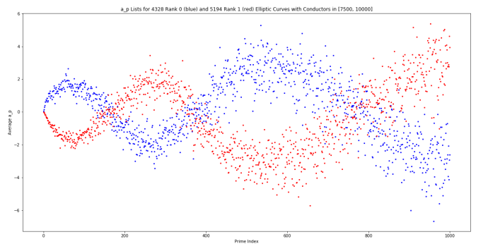
(a) Rank bias observed in [3] (with authors’ permission)

(b) Starlings murmurations. AlbertoGonzalez/Shutterstock.com

Later, Sutherland and the authors ([13], [4]) detected this bias in more general families of arithmetic $L$ functions, for instance, those associated to weight $k$ holomorphic modular cusp forms for $\Gamma_{0}(N)$ with conductor in a geometric interval range $[M,cM]$ and a fixed root number. Sutherland made a striking observation that the average of $a_{f}(P)$ over this family for a single prime $P\sim M$ converges a continuous-looking function of $P/M$:

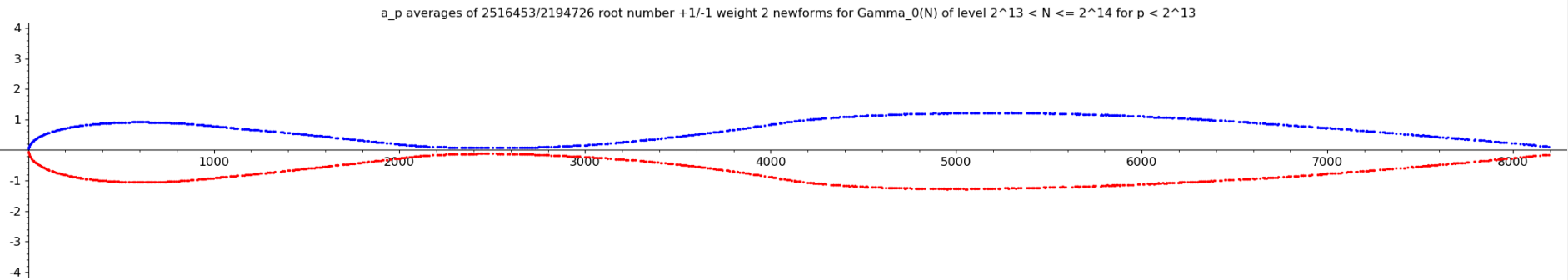
Figure 2: Dyadic averages of $a(p)$ with a fixed root number, courtesy of Sultherland

The goal of this paper is to establish this bias in families of modular forms of square-free level with arbitrary fixed weight and root number. We show the following:

Theorem 1.

Let $H^{\text{new}}(N)$ be a Hecke basis for trivial character weight $k$ cusp newforms for $\Gamma_{0}(N)$ with $f\in H^{\text{new}}(N)$ normalized to have lead coefficient $1$. Let $\varepsilon(f)$ be the root number of $f$, let $a_{f}(p)$ be the $p$-th Fourier coefficient of $f$, and let $\lambda_{f}(p):=a_{f}(p)/p^{(k-1)/2}$. Let $X,Y,$ and $P$ be parameters going to infinity with $P$ prime; assume further that that $Y=(1+o(1))X^{1-\delta_{2}}$ and $P\ll X^{1+\delta_{1}}$ for some $\delta_{2},\delta_{1}>0$ with $2\delta_{1}<\delta_{2}<1$. Let $y:=P/X$. Then:

$$\frac{\sum^{\square}_{\begin{subarray}{I}N\in[X,X+Y]\end{subarray}}\sum_{f\in H^{\text{new}}(N)}\lambda_{f}(P)\sqrt{P}\varepsilon(f)}{\sum^{\square}_{\begin{subarray}{I}N\in[X,X+Y]\end{subarray}}\sum_{f\in H^{\text{new}}(N,k)}1} =D_{k}A\sqrt{y}+(-1)^{k/2-1}D_{k}B\sum_{1\leq r\leq 2\sqrt{y}}c(r)\sqrt{4y-r^{2}}U_{k-2}\left(\frac{r}{2\sqrt{y}}\right)$$

$$-D_{k}\delta_{k=2}\pi y+\mathrm{O}_{\varepsilon}\left(X^{-\delta^{\prime}+\varepsilon}+\frac{1}{P}\right)$$

where $U_{k-2}$ is the Chebyshev polynomial given by

$$U_{n}(\cos\theta):=\frac{\sin((n+1)\theta)}{\sin\theta},$$

$$\delta^{\prime}:=\min\{\delta_{2}/2-\delta_{1},1/9+\delta_{2}/9-\delta_{1}\},$$

$$A:=\prod_{p}\left(1+\frac{p}{(p+1)^{2}(p-1)}\right),$$

$$B:=\prod_{p}\frac{p^{4}-2p^{2}-p+1}{(p^{2}-1)^{2}},$$

$$D_{k}:=\frac{12}{(k-1)\pi\prod_{p}\left(1-\frac{1}{p^{2}+p}\right)},$$

$$c(r):=\prod_{p|r}\left(1+\frac{p^{2}}{p^{4}-2p^{2}-p+1}\right),$$

and $\sum^{\square}$ denotes a sum over square-free parameters. In particular, for any $\delta_{1}<2/9$, one can find $\delta_{2}$ for which $\delta^{\prime}>0$.

We define

$$M_{k}(y):=D_{k}A\sqrt{y}+(-1)^{k/2-1}D_{k}B\sum_{1\leq r\leq 2\sqrt{y}}c(r)\sqrt{4y-r^{2}}U_{k-2}\left(\frac{r}{2\sqrt{y}}\right)-D_{k}\delta_{k=2}\pi y$$

to be the weight $k$ murmuration density.

The formula above arises from an application of the Eichler-Selberg trace formula to the composition of Hecke and Atkin-Lehner operators, which allows us to reinterpret the sum in terms of class numbers. We then compute class number averages in short intervals by means of the class number formula.

We remark that the exponents in the statement are far from optimal, as our goal here is only to get a power saving error term in a range up to $X^{a}$ for some $a>1$. The restriction to square-free levels is a technical one, as the trace formula simplifies greatly when the level is square-free. From the computations of Sutherland, it appears that the resulting density functions are slightly perturbed when one considers all levels, but they share key properties with the ones above.

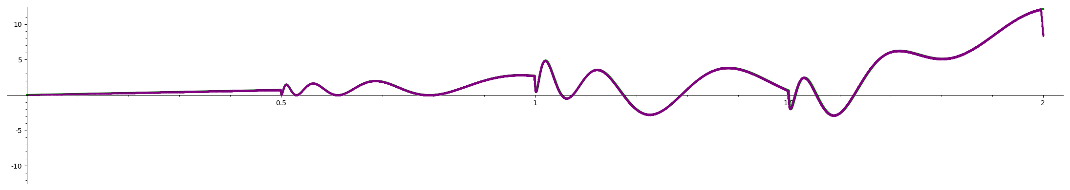
Figure 3: Plots of $M_{8}$ and $M_{24}$, courtesy of Sultherland ([14])

The murmuration densities $M_{k}(y)$ in Theorem 1 have many interesting features. They are highly oscillating, continuous, with derivative discontinuities at $n^{2}/4$ for $n\in\mathbb{N}$. At the origin, the $M_{k}$’s are positive and grow like $\sqrt{y}$. This positive root number bias for small $P$ has been observed previously in the works of Martin and Pharis (see [8], [9], [10]).

In the case of weight $k=2$, we analyze the behavior this function as $y\to\infty$ in more detail. In spite of the appearing $y$ term, it has a true growth rate of $y^{1/4}$. The function $M_{2}(y)/y^{1/4}$ is an asymptotically uniformly almost periodic function of $\sqrt{y}$; it is a convergent sum of periodic functions with (increasing) half integer periods. Its sign, i.e., the sign of the correlation bias, changes infinitely often. We prove the following:

Theorem 2.

Let

$$M_{2}(y)=D_{2}A\sqrt{y}+D_{2}B\sum_{1\leq r\leq 2\sqrt{y}}c(r)\sqrt{4y-r^{2}}-D_{2}\pi y$$

be the weight $2$ murmuration density. Then as $y\to\infty$,

$$M_{2}(y)=y^{1/4}\cdot\frac{2BD_{2}}{\pi}\sum_{\begin{subarray}{I}1\leq d\leq 2\sqrt{y}\\ d\ \square\text{-free }\end{subarray}}Q(d)d^{1/2}\zeta\left(-1/2,\left\{\frac{2\sqrt{y}}{d}\right\}\right)+\mathrm{O}(1).$$

Here $\zeta$ is the Hurwitz zeta function,

$$Q(d):=\prod_{p|d}\frac{p^{2}}{p^{4}-2p^{2}-p+1}\asymp\mu^{2}(d)/d^{2}$$

and $\{\cdot\}$ denotes the fractional part.

Figure 4: The weight $2$ density function

Integrating the murmuration density above produces the dyadic interval weight $k$ averages observed by Sutherland:

Theorem 3.

Let $P\ll X^{6/5}$, let $c>1$ be a constant, $Z:=cX,$ and $y:=P/X$. Then as $X\to\infty,$

$$\frac{\sum^{\square}_{\begin{subarray}{I}N\in[X,Z]\end{subarray}}\sum_{f\in H^{\text{new}}(N,k)}\lambda_{f}(P)\sqrt{P}\varepsilon(f)}{\sum^{\square}_{\begin{subarray}{I}N\in[X,Z]\end{subarray}}\sum_{f\in H^{\text{new}}(N,k)}1}=\frac{2}{(c^{2}-1)}\int_{1}^{c}uM_{k}(y/u)du+o_{y}(1),$$

where $M_{k}(y)$ is as in Theorem 1. In particular, for $k=c=2$, the dyadic average

$$\frac{\sum^{\square}_{\begin{subarray}{I}N\in[X,2X]\end{subarray}}\sum_{f\in H^{\text{new}}(N,1)}a_{f}(P)\varepsilon(f)}{\sum^{\square}_{\begin{subarray}{I}N\in[X,2X]\end{subarray}}\sum_{f\in H^{\text{new}}(N,k)}1}$$

converges to

$$\begin{cases}\alpha\sqrt{y}-\beta y&\text{on }[0,1/4];\\ \alpha\sqrt{y}-\beta y+\gamma\pi y^{2}-\gamma(1-2y)\sqrt{y-1/4}-2\gamma y^{2}\arcsin(1/2y-1))&\text{on }[1/4,1/2];\\ \alpha\sqrt{y}-\beta y+2\gamma y^{2}(\arcsin(1/y-1)-\arcsin(1/2y-1))\\ \hskip 54.92479pt-\gamma(1-2y)\sqrt{y-1/4}+2\gamma(1-y)\sqrt{2y-1}&\text{on }[1/2,1],\end{cases}$$

where

$$\alpha\approx 6.38936,\beta\approx 11.3536,\gamma\approx 2.6436.$$

We note this is the function from Figure 2.

Finally, we analyze the asymptotic behavior of the smoothed averages from Theorem 3:

Theorem 4.

Let $\Phi:(0,\infty)\to\mathbb{C}$ be a compactly supported smooth weight function, and let

$$M_{\Phi}(y):=\Big{(}\int_{0}^{\infty}M_{2}(y/u)\Phi(u)u^{2}\frac{du}{u}\Big{)}/\int_{0}^{\infty}\Phi(u)u^{2}\frac{du}{u}.$$

Then $M_{\Phi}$ is continuous on $(0,\infty)$, $M_{\Phi}(0)=0$, and as $y\to\infty$,

$$M_{\Phi}(y)=1+o_{y}(1).$$

Asymptotic properties of the characteristic function averages as in Theorem 3 will be analyzed in forthcoming work.

Murmurations are a feature of the the one-level density transition range. The Katz-Sarnak philosophy ([6]) predicts that averages as in Theorem 4 for $P\sim N^{a}$ behave differently when $a<1$ and $a>1$, and our statements for $P\sim N$ describe the phase transition between these. The unusual (for $k>2$) normalization of the coefficients above also arises naturally from this interpretation. For a more detailed discussion of this connection, we point the reader to [11].

Computing similar averages weighted "harmonically" (i.e., by the value at $1$ of the symmetric square $L$-function) by means of the Petersson formula reveals that with weights, this bias becomes much less pronounced: the resulting function grows like $y$, as opposed to $\sqrt{y}$, at the origin.

Murmurations for elliptic curves over $\mathbb{Q}$ are not explained by these results, as they constitute a very sparse subset of weight $2$ modular forms. We point out that computational observations of the aforementioned authors make a compelling case that this phenomenon is very sensitive to the ordering by conductor, and disappears almost entirely when the curves are ordered by naive height, $j$-invariant, or discriminant.

2 Trace Formula Setup

Given a square-free positive integer $N$ and a prime $P\nmid N$, let $H^{\text{new}}(N,k)$ denote a basis of the space $S^{\text{new}}(N,k)$ of weight $k$ Hecke cusp newforms for $\Gamma_{0}(N)$, and let $a_{f}(P)=\lambda_{f}(P)P^{(k-1)/2}$ denote the eigenvalue under the $P$-th Hecke operator $T_{p}$ of $f\in H^{\text{new}}(N,k)$. Let $\varepsilon(f)$ denote the root number of $f$ (recall $(-1)^{k/2}\varepsilon(f)$ is equal to the eigenvalue of $f$ under the Atkin-Lehner involution $W_{N}$). In order to compute the average of $a_{f}(P)\varepsilon(f)$ for eigenforms $f$ ranging over square-free levels $N$ in an interval, we interpret $\sum_{f\in H^{\text{new}}(N,k)}a_{f}(P)\varepsilon(f)$ as the trace of the operator $(-1)^{k/2}T_{p}\circ W_{N}$ on $S^{\text{new}}(N)$ and apply the corresponding trace formula.

Such a trace formula was first derived by Yamauchi in [16]; the result contained a computational error which was later corrected by Skoruppa and Zagier ([12]). This formula (section $2$, formula ($7$)) gives the trace of $T_{p}\circ W_{N}$ on the full space of cusp forms $S(N)$; as the authors point out in the discussion leading to formula $(5)$, oldforms coming from $S(M)$ contribute to the trace only when $N/M$ is a square. Since we are restricting ourselves to $N$ square-free, we thus have the following result at our disposal:

Theorem (Skoruppa-Zagier ([12], section $2$, formulas ($5$) and ($7$)).

For $N$ square-free and a prime $P\nmid N$,

$$\sum_{f\in H^{\text{new}}(N,k)}\sqrt{P}\lambda_{f}(P)\varepsilon(f) =\frac{H_{1}(-4PN)}{2}+(-1)^{k/2-1}U_{k-2}\left(\frac{r\sqrt{N}}{2\sqrt{P}}\right)\sum_{0<r\leq 2\sqrt{P/N}}H_{1}(r^{2}N^{2}-4PN)$$

$$-\delta_{k=2}(P+1).$$

Here the Hurwitz class number $H_{1}(-d)$ is the number of equivalence classes with respect to $\operatorname{SL}_{2}(\mathbb{Z})$ of positive-definite binary quadratic forms of discriminant $-d$ weighed by the number of automorphisms (i.e., with forms corresponding to multiples of $x^{2}+y^{2}$ and $x^{2}+xy+y^{2}$ counted with multiplicities $1/2$ and $1/3$, accordingly). Hence, $H_{1}$ can be expressed in terms of the Gauss class number $h$ via:

$$H_{1}(-d)=\sum_{f\in\mathbb{N}:f^{2}|d}h(-d/f^{2})+\mathrm{O}(1),$$

with the error term disappearing if $d\neq 3\cdot\square,4\cdot\square$.

Assume from now on that $P\neq 2$. The square factors of $4PN$ are $1$ and $4$, since by assumption $P\nmid N$. For a prime $q$ and $r\geq 1$, the condition $q^{2}\mid N(r^{2}N-4P)$ can hold either if $q^{2}|r^{2}N-4P$ or if $q$ divides both $N$ and $4P$, i.e., if $q=2$ and $N$ is even. However, if $N=2N^{\prime}$ is even (with $N^{\prime}$ odd), then for any $d$ with $4d^{2}|(r^{2}N^{2}-4PN)$, one has

$$(r^{2}N^{2}-4PN)/4d^{2}=(r^{2}N^{\prime 2}-2PN^{\prime})/d^{2},$$

which is always $2$ or $3$ modulo $4$, so the corresponding class number vanishes. Thus it suffices to consider square divisors of $r^{2}N^{2}-4PN$ for which $d^{2}|r^{2}N-4P$. Consequently, for $N$ square-free, and a prime $P\nmid 2N$, the trace formula becomes:

$$\sum_{f\in H^{\text{new}}(N)}\sqrt{P}\lambda_{f}(P)\varepsilon(f) =\frac{h(-4PN)}{2}+\frac{h(-PN)}{2}-\delta_{k=2}P+\mathrm{O}(1).$$

$$+(-1)^{k/2-1}U_{k-2}\left(\frac{r\sqrt{N}}{2\sqrt{P}}\right)\sum_{1\leq r\leq 2\sqrt{\frac{P}{N}}}\sum_{d^{2}|r^{2}N-4P}h(N(r^{2}N-4P)/d^{2}).$$ (1)

From this formula, one can already see that the trace is positively biased, at least for small $P$. Indeed, the only negative term in this expression is $-P$; on the other hand, Siegel’s bound dictates that the class number terms should be of size $(PN)^{1/2+\varepsilon}$, which dominates for small $P$, as was observed in ([8]) and ([9]), ([10]).

On the other hand, for $P$ of size $N^{1+\varepsilon}$, the balance becomes more subtle, and as we will see, the trace can be either positive or negative, even when averaged over short intervals in $N$.

3 Average Class Number in Short Intervals

Our interest in this section is to exploit the Dirichlet class number formula to understand sums of class numbers in (2) as the square-free parameter $N$ ranges over a short interval $[X,X+Y]$ for $Y=o(X)$. For such an interval, the square root term in the class number formula has fixed size, so these sums can be understood by averaging Dirichlet characters coming from a truncated $L$ function special value. Carrying out this computation yields Theorem 1. We establish it via the following two propositions:

Proposition 3.1.

Let $P\neq 2$ be prime and let $[X,X+Y]$ be an interval of length $Y=o(X)$. Then as $X\to\infty$, we have

$$\frac{\zeta(2)\pi}{XY}\sideset{}{{}^{\square}}{\sum}_{\begin{subarray}{I}N\in[X,X+Y]\\ P\nmid N\end{subarray}}\frac{h(-PN)}{2}+\frac{h(-4PN)}{2}=A\sqrt{y}+\mathrm{O}_{\varepsilon}\left(\frac{1}{P^{3/2}X^{1/2}}+\frac{P^{7/12}}{Y^{5/6}X^{5/12}}+\frac{YP^{1/2}}{X^{3/2}}\right)(XYP)^{\varepsilon}.$$

Here the error term is $o(y)$ as long as $P\to\infty$, $Y=o(X/\log(PX))$, and for some $\varepsilon>0$, $X^{7/10+\varepsilon}P^{1/10+\varepsilon}=o(Y)$.

Proposition 3.2.

Let $P\neq 2$ be a prime, let $r\in\mathbb{N}$, and let $X>Y>0$ be such that $r^{2}(X+Y)<4P$ for each integer $r<2\sqrt{P/X}$. Then:

$$\frac{\zeta(2)\pi}{YX}\sum_{r\leq 2\sqrt{P/X}}\sideset{}{{}^{\square}}{\sum}_{\begin{subarray}{I}N\in[X,X+Y]\\ P\nmid N\end{subarray}}H_{1}(r^{2}N^{2}-4PN)=\sum_{r\leq 2\sqrt{P/X}}c(r)\sqrt{4y-r^{2}}$$

$$+\mathrm{O}\Big{(}\frac{P^{11/10}}{Y^{2/5}X^{9/10}}+\frac{YP}{X^{2}}+\frac{PY^{1/2}}{X^{3/2}}+\frac{P}{\sqrt{X}Y^{13/18}}+\frac{P}{XY^{1/9}}\Big{)}(XYP)^{\varepsilon}.$$

Subsections 3.1 proves Proposition 3.1. In subsection 3.2, we prove Proposition 3.2 by adapting the same idea to the more complex square divisor structure of the arguments of the class numbers involved.

3.1 $H_{1}(-4PN)$

3.1.1 $h(-PN)$

By Dirichlet’s class number formula, for $d>4$, $h(-d)$ is $0$ if $-d=2$ or $3\hskip 1.4457pt\mathrm{mod}\hskip 1.4457pt4$, and otherwise

$$h(-d)=\frac{\sqrt{d}}{\pi}L(1,\chi_{d}),$$

where $L(1,\chi_{d})$ is the value at $1$ of the Dirichlet series for the Kronecker symbol $\left(\frac{d}{n}\right)$ (a quadratic Dirichlet character of modulus $d$ or $4d$). We evaluate the sum

$$\frac{1}{\sqrt{PX}}\sum_{N\in[X,X+Y]}h(-PN)=\frac{1}{\pi}\sum_{\begin{subarray}{I}N\in[X,X+Y]\\ PN=3\hskip 1.4457pt\mathrm{mod}\hskip 1.4457pt4\end{subarray}}\sqrt{N/X}L(1,\chi_{-PN}).$$ (2)

by truncating the Dirichlet series of the $L$-function and splitting the corresponding characters into primitive and non-primitive ones. For $\chi$ a non-principal Dirichlet character of modulus $d$, it follows from Abel summation and Polya-Vinogradov that for a truncation parameter $T$,

$$L(1,\chi)=\sum_{n\geq 1}\frac{\chi(n)}{n}=\sum_{n=1}^{T}\frac{\chi(n)}{n}+\mathrm{O}\left(\sqrt{d}\log d/T\right)$$ (3)

(see, for example, [1], page $321$, Theorem $5.2$.) Since $\chi_{-PN}$ is always a non-principal Dirichlet character for square-free $N$ with $P\nmid N$, we have

$$\sum_{\begin{subarray}{I}N\in[X,X+Y]\\ PN=3\hskip 1.4457pt\mathrm{mod}\hskip 1.4457pt4\end{subarray}}\sqrt{N/X}L(1,\chi_{-PN})=\sum_{\begin{subarray}{I}N\in[X,X+Y]\\ PN=3\hskip 1.4457pt\mathrm{mod}\hskip 1.4457pt4\end{subarray}}\sqrt{N/X}\sum_{n=1}^{T}\frac{\left(\frac{-PN}{n}\right)}{n}+\mathrm{O}\left(\frac{Y\sqrt{PX}\log PX}{T}\right)$$

$$= \sum_{\begin{subarray}{I}N\in[X,X+Y]\\ PN=3\hskip 1.4457pt\mathrm{mod}\hskip 1.4457pt4\end{subarray}}\sum_{m=1}^{\sqrt{T}}\frac{\sqrt{N/X}\left(\frac{-PN}{m^{2}}\right)}{m^{2}}+\sum_{\begin{subarray}{I}N\in[X,X+Y]\\ PN=3\hskip 1.4457pt\mathrm{mod}\hskip 1.4457pt4\end{subarray}}\sum_{\begin{subarray}{I}n=1\\ n\neq\square\end{subarray}}^{T}\frac{\sqrt{N/X}\left(\frac{-PN}{n}\right)}{n}+\mathrm{O}\left(\frac{Y\sqrt{PX}\log PX}{T}\right)$$

$$=: \mathrm{Sq}+\mathrm{NSq}+\mathrm{O}\left(\frac{Y\sqrt{PX}\log PX}{T}\right).$$

Since the sum $\mathrm{Sq}$ contains principal characters and $\mathrm{NSq}$ is going over non-principal ones, we expect $\mathrm{Sq}$ to be the main term. Indeed,

$$\mathrm{Sq} =\sum_{m=1}^{\sqrt{T}}\frac{1}{m^{2}}\sum_{\begin{subarray}{I}N\in[X,X+Y]\\ PN=3\hskip 1.4457pt\mathrm{mod}\hskip 1.4457pt4\end{subarray}}\mu^{2}(N)\left(\frac{-PN}{m^{2}}\right)\Big{(}1+\Big{(}\sqrt{1+\frac{N-X}{X}}-1\Big{)}\Big{)}$$

$$=\sum_{m=1}^{\sqrt{T}}\frac{1}{m^{2}}\sum_{\begin{subarray}{I}N\in[X,X+Y]\\ PN=3\hskip 1.4457pt\mathrm{mod}\hskip 1.4457pt4\end{subarray}}\mu^{2}(N)\left(\frac{-PN}{m^{2}}\right)+O\left(Y\left(\sqrt{1+Y/X}-1\right)\right)$$

$$=\sum_{\begin{subarray}{I}m\leq\sqrt{T}\\ (P,m)=1\end{subarray}}\frac{1}{m^{2}}\left(\sum_{\begin{subarray}{I}N\in[X,X+Y]\end{subarray}}\mu^{2}(N)\left(\frac{N}{m^{2}}\right)\frac{\chi_{1}(PN)-\chi_{2}(PN)}{2}\right)+O\left(\frac{Y^{2}}{X}\right)$$

where $\chi_{1,2}$ are the characters modulo $4$, $\chi_{1}$ principal. The character $\left(\frac{N}{m^{2}}\right)\chi_{1}(N)$ is principal modulo $2m$, and $\left(\frac{N}{m^{2}}\right)\chi_{2}(N)$ is always non-principal modulo $4m$. Applying Lemmas 6.7 and Lemma 6.5,

$$\mathrm{Sq} =\sum_{\begin{subarray}{I}m\leq\sqrt{T}\\ (P,m)=1\end{subarray}}\frac{Y}{\zeta(2)}\frac{\eta(2m)}{2m^{2}}+O_{\varepsilon}\left(\frac{1}{m^{2}}m^{1/5+\varepsilon}X^{3/5+\varepsilon}\right)+O\left(\frac{Y^{2}}{X}\right)$$

$$=Y\frac{4A}{11\zeta(2)}+\mathrm{O}_{\varepsilon}\left(\frac{Y}{P^{2}}+\frac{Y}{\sqrt{T}}+X^{3/5+\varepsilon}+\frac{Y^{2}}{X}\right).$$ (4)

Next, we want to bound the term

$$\mathrm{NSq} =\sum_{\begin{subarray}{I}N\in[X,X+Y]\\ PN=3\hskip 1.4457pt\mathrm{mod}\hskip 1.4457pt4\end{subarray}}\sum_{\begin{subarray}{I}n=1\\ n\neq\square\end{subarray}}^{T}\frac{\sqrt{N/X}\left(\frac{-PN}{n}\right)}{n}=\sum_{\begin{subarray}{I}N\in[X,X+Y]\\ PN=3\hskip 1.4457pt\mathrm{mod}\hskip 1.4457pt4\end{subarray}}\sum_{\begin{subarray}{I}n=1\\ n\neq\square\end{subarray}}^{T}\frac{\left(\frac{-PN}{n}\right)}{n}+O\left(\frac{Y^{2}\sum_{n\leq T}(1/n)}{X}\right)$$

$$=\sum_{\begin{subarray}{I}n=1\\ n\neq\square\end{subarray}}^{T}\frac{\left(\frac{-P}{n}\right)}{n}\left(\sum_{\begin{subarray}{I}N\in[X,X+Y]\end{subarray}}\left(\frac{N}{n}\right)\frac{\chi_{1}(PN)-\chi_{2}(PN)}{2}\right)+O\left(\frac{Y^{2}\log T}{X}\right)$$

For $n$ not a square, $\left(\frac{N}{n}\right)$ is non-principal; moreover, $\left(\frac{N}{2}\right)$ is primitive modulo $8$. Hence $\left(\frac{N}{n}\right)\chi_{1,2}(N)$ are also non-principal, so applying Lemma 6.7 again,

$$\mathrm{NSq}=\sum_{\begin{subarray}{I}n=1\\ n\neq\square\end{subarray}}^{T}(1/n)\mathrm{O}_{\varepsilon}\left(n^{1/5+\varepsilon}X^{3/5+\varepsilon}\right)+O\left(Y^{2}\log T/X\right)\ll_{\varepsilon}T^{1/5+\varepsilon}X^{3/5+\varepsilon}+Y^{2}\log T/X.$$ (5)

Combining (2), (3.1.1), and (5),

$$\frac{1}{\sqrt{PX}}\sum_{N\in[X,X+Y]}h(-PN)=\frac{4A}{11\zeta(2)\pi}Y+\mathrm{Err}_{Y,X,P,T},$$ (6)

where

$$\mathrm{Err}_{Y,X,P,T}=\mathrm{O}_{\varepsilon}\left(\frac{Y}{P^{2}}+\frac{Y}{\sqrt{T}}+X^{3/5+\varepsilon}T^{1/5+\varepsilon}+\frac{Y^{2}\log T}{X}+\frac{Y\sqrt{PX}\log PX}{T}\right).$$

In particular, setting $T:=Y^{5/6}P^{5/12}X^{-1/12}$, we get an error term matching that of Proposition 3.1.

3.1.2 $h(-4PN)$

We handle this case the same way as in the previous section. Since $-4PN$ is always $0\hskip 1.4457pt\mathrm{mod}\hskip 1.4457pt4$,

$$\frac{1}{\sqrt{PX}}\sum_{N\in[X,X+Y]}h(-4PN) =\frac{2}{\pi}\sum_{\begin{subarray}{I}N\in[X,X+Y]\end{subarray}}\sqrt{\frac{N}{X}}L(1,\chi_{-4PN})$$

$$=\frac{2}{\pi}\sum_{\begin{subarray}{I}N\in[X,X+Y]\end{subarray}}\sqrt{\frac{N}{X}}\sum_{n=1}^{T}\frac{\left(\frac{-4PN}{n}\right)}{n}+\mathrm{O}\left(\frac{Y\sqrt{PX}\log PX}{T}\right)$$

$$=\frac{2}{\pi}\sum_{\begin{subarray}{I}N\in[X,X+Y]\end{subarray}}\sum_{n=1}^{T}\frac{\left(\frac{-4PN}{n}\right)}{n}+\mathrm{O}\left(\frac{Y\sqrt{PX}\log PX}{T}+\frac{Y^{2}\log T}{X}\right).$$

Again, we can separate into principal and non-principal characters:

$$\sum_{\begin{subarray}{I}N\in[X,X+Y]\end{subarray}}\sum_{n=1}^{T}\frac{\left(\frac{-4PN}{n}\right)}{n}=\sum_{\begin{subarray}{I}n=1\\ n\neq\square\\ n\text{ odd }\end{subarray}}^{T}\sum_{\begin{subarray}{I}N\in[X,X+Y]\end{subarray}}\frac{\left(\frac{-PN}{n}\right)}{n}+\sum_{\begin{subarray}{I}m=1\\ m\text{ odd }\end{subarray}}^{\sqrt{T}}\sum_{N\in[X,X+Y]}\frac{\left(\frac{-PN}{m^{2}}\right)}{m^{2}}$$

Applying Lemma 6.7 and Lemma 6.5 as in the previous section, we conclude

$$\frac{1}{\sqrt{PX}}\sum_{N\in[X,X+Y]}h(-4PN)=\frac{2Y}{\pi\zeta(2)}\left(\sum_{\begin{subarray}{I}m\text{ odd }\\ (m,P)=1\end{subarray}}^{\sqrt{T}}\frac{\eta(m)}{m^{2}}\right)Y+\mathrm{Err}_{Y,X,P,T}=Y\frac{18A}{11\zeta(2)\pi}+\mathrm{Err}_{Y,X,P,T},$$

which finishes the proof of Proposition 3.1 in combination with (6).

3.2 $H_{1}(r^{2}N^{2}-4PN$)

The aim of this section is to prove the following:

Proposition 3.3.

Let $P\neq 2$ be a prime, let $r\in\mathbb{N}$, and let $X>Y>0$ be such that $r^{2}(X+Y)<4P.$ Then:

$$\sideset{}{{}^{\square}}{\sum}_{\begin{subarray}{I}N\in[X,X+Y]\\ P\nmid N\end{subarray}}H_{1}(r^{2}N^{2}-4PN)=\frac{YBc(r)}{\pi\zeta(2)}\sqrt{4PX-r^{2}X^{2}}$$

$$+\mathrm{O}\left(YPX)^{\varepsilon}\Big{(}(YPX)^{3/5}+\frac{Y^{2}\sqrt{P}}{\sqrt{X}}+rY^{3/2}X^{1/2}+X\sqrt{P}Y^{5/18}+Y^{8/9}\sqrt{PX}\Big{)}\right).$$

For a divisor $d^{2}|r^{2}N-4P$ such that $\frac{r^{2}N^{2}-4PN}{d^{2}}=0/1\hskip 1.4457pt\mathrm{mod}\hskip 1.4457pt4$, we once again have by the class number formula that

$$h\left(\frac{r^{2}N^{2}-4PN}{d^{2}}\right)=\frac{\sqrt{4PN-r^{2}N^{2}}}{\pi d}L(1,\chi_{\frac{r^{2}N^{2}-4PN}{d^{2}}}).$$

Thus, for $1\leq r\leq 2\sqrt{P/(X+Y)}$,

$$\sideset{}{{}^{\square}}{\sum}_{\begin{subarray}{I}N\in[X,X+Y]\\ P\nmid N\end{subarray}}H_{1}(r^{2}N^{2}-4PN)=\sum_{\begin{subarray}{I}d^{2}\leq 4P\end{subarray}}\sum_{\begin{subarray}{I}N\in[X,X+Y]\\ N\in\widetilde{\mathcal{A}}_{r,d}\end{subarray}}\frac{L(1,\chi_{(r^{2}N^{2}-4PN)/d^{2}})}{\pi d}\sqrt{4PN-r^{2}N^{2}},$$

where we let

$$\widetilde{\mathcal{A}}_{k,d}:=\{N\in\mathbb{Z}:N\ \square\text{ - free},P\nmid N,d^{2}|r^{2}N-4P,\text{ and }(r^{2}N^{2}-4PN)/d^{2}\equiv 0/1\hskip 1.4457pt\mathrm{mod}\hskip 1.4457pt4.\}$$

We begin by analyzing the set $\widetilde{\mathcal{A}}_{r,d}$.

3.2.1 Remainder analysis

Suppose first that $r$ is odd. For $N$ square-free, $d^{2}|r^{2}N-4P$ implies that $d$ is odd, and $\frac{r^{2}N^{2}-4PN}{d^{2}}\equiv 0/1\hskip 1.4457pt\mathrm{mod}\hskip 1.4457pt4$ automatically holds. Thus, $\widetilde{\mathcal{A}}_{r,d}$ is the set of square-free integer solutions to the congruence

$$r^{2}N=4P\hskip 1.4457pt\mathrm{mod}\hskip 1.4457ptd^{2},P\nmid N.$$

For odd $r$ and $d$, this has a solution if and only if $P\nmid d$ and $(r,d)=1$, yielding

$$\widetilde{\mathcal{A}}_{r,d}=\{N\in\mathcal{A}_{r,d}:N\ \square\text{ - free},P\nmid N\},$$

where we let

$$\mathcal{A}_{r,d}:=\begin{cases}n\in\mathbb{Z}:n\equiv 4Pk^{-2}\hskip 1.4457pt\mathrm{mod}\hskip 1.4457ptd^{2}&\text{ if }(d,r)=(d,P)=(d,2)=1;\\ \emptyset&\text{ otherwise}\end{cases}$$

Now assume $r$ is even. From $d^{2}|4P-r^{2}N<4P$ and since $r^{2}X<4P$, we know $r,d<P$, i.e., $(P,k)=(P,d)=1.$ Let $r:=2l$. Then $\frac{r^{2}N^{2}-4PN}{d^{2}}=0/1\hskip 1.4457pt\mathrm{mod}\hskip 1.4457pt4$ is equivalent to

$$4l^{2}N=4P+rd^{2}\hskip 1.4457pt\mathrm{mod}\hskip 1.4457pt4d^{2},\text{ where }rN=0/1\hskip 1.4457pt\mathrm{mod}\hskip 1.4457pt4.$$ (7)

If $d$ is odd, reducing (7) modulo $4$ shows that $r\equiv 0\hskip 1.4457pt\mathrm{mod}\hskip 1.4457pt4$, and (7) simplifies to

$$l^{2}N=P\hskip 1.4457pt\mathrm{mod}\hskip 1.4457ptd^{2}.$$

This has $1$ solution $\hskip 1.4457pt\mathrm{mod}\hskip 1.4457ptd^{2}$ for $(l,d)=1$ and no solutions otherwise. Suppose now $d=2b$, so (7) becomes

$$l^{2}N=P+rb^{2}\hskip 1.4457pt\mathrm{mod}\hskip 1.4457pt4b^{2},rN=0/1\hskip 1.4457pt\mathrm{mod}\hskip 1.4457pt4.$$ (8)

Since we restrict to $N$ square-free, we can disregard the case $N\equiv 0\hskip 1.4457pt\mathrm{mod}\hskip 1.4457pt4$. If $N=2\hskip 1.4457pt\mathrm{mod}\hskip 1.4457pt4$, then $r$ must be even and (8) has no solutions $\hskip 1.4457pt\mathrm{mod}\hskip 1.4457pt2$. For $N$ odd, $rN=0/1\hskip 1.4457pt\mathrm{mod}\hskip 1.4457pt4$ holds if and only if $r=0/N\hskip 1.4457pt\mathrm{mod}\hskip 1.4457pt4$, and we have an equivalence

$$(\ref*{equat})\ \&\ N\text{ is odd }\iff\left[\begin{array}[]{@{}l@{\quad}l@{}}N(l^{2}-b^{2})=P\hskip 1.4457pt\mathrm{mod}\hskip 1.4457pt4b^{2},N\text{ odd}\\ Nl^{2}=P\hskip 1.4457pt\mathrm{mod}\hskip 1.4457pt4b^{2},N\text{ odd}.\end{array}\right.$$

If $(l,b)>1$, this has no solutions since $P\nmid(l,b)$. Otherwise, if $(l,b)=1$, there are three cases:

• if $l,b$ are odd, there is a solution $N\equiv Pl^{-2}\hskip 1.4457pt\mathrm{mod}\hskip 1.4457pt4b^{2};$

• if $l$ is even, $b$ is odd, there is a solution $N\equiv P(l^{2}-b^{2})^{-1}\hskip 1.4457pt\mathrm{mod}\hskip 1.4457pt4b^{2};$

• if $l$ is odd, $b$ is even, there’s a solution $N\equiv Pl^{-2}\hskip 1.4457pt\mathrm{mod}\hskip 1.4457pt4b^{2}$ and a solution $N=P(l^{2}-b^{2})^{-1}\hskip 1.4457pt\mathrm{mod}\hskip 1.4457pt4b^{2}$, distinct.

Note $N$ is automatically odd in the above three cases.

In summary, for any choice of $r$ and $d$,

$$\widetilde{\mathcal{A}}_{r,d}:=\{N\in\mathcal{A}_{r,d}:P\nmid N,N\ \square\text{ - free}\},$$

where the set $\mathcal{A}_{r,d}$ is given by a congruence condition modulo $d^{2}$; namely,

$$\mathcal{A}_{r,d}:=\{n\in\mathbb{Z}:n\hskip 1.4457pt\mathrm{mod}\hskip 1.4457ptd^{2}\in\mathcal{R}_{d,r},\}$$

where $\mathcal{R}_{d,r}$ is a subset of residues mod $d^{2}$ coprime to $d$ that satisfies:

$$\absolutevalue{\mathcal{R}_{d,r}}=\begin{cases}1&\text{ if }(d,r)=1,2\nmid d,k,P\nmid d\\ 1&\text{ if }(d,r)=1,2|r\\ 1&\text{ if }(d,r)=2,2||d;\\ 2&\text{ if }(d,r)=2,4|d;\\ \emptyset&\text{ otherwise}.\end{cases}$$

Furthermore, letting $s:=\frac{r^{2}N^{2}-4PN}{d^{2}}$ for some $N\in\mathcal{A}_{r,d}$, the above analysis also proves that:

• For $(d,r)=2,2||d,2||r,$ $s$ is always even;

• For $(d,r)=2,2||d,4|r,$ $s$ is always odd;

• For $(d,r)=2,4|d$, the two residues in $\mathcal{R}_{r,d}$ produce $s$ of different parity.

We will call a pair $(r,d)$ admissible if $\mathcal{R}_{r,d}$ is non-empty.

3.2.2 Truncation

We have established that

$$\sideset{}{{}^{\square}}{\sum}_{\begin{subarray}{I}N\in[X,X+Y]\\ P\nmid N\end{subarray}}H_{1}(r^{2}N^{2}-4PN) =\sum_{\begin{subarray}{I}d^{2}\leq 4P\ \ \end{subarray}}\sideset{}{{}^{\square}}{\sum}_{\begin{subarray}{I}N\in[X,X+Y]\\ N\in{\mathcal{A}}_{r,d}\\ P\nmid N\end{subarray}}\frac{L(1,\chi_{\frac{r^{2}N^{2}-4PN}{d^{2}}})}{\pi d}\sqrt{4PN-r^{2}N^{2}}.$$ (9)

Note that for $N\in[X,X+Y]$ (and assuming $r^{2}(X+Y)<4P$),

$$\sqrt{4PN-r^{2}N^{2}}-\sqrt{4PX-r^{2}X^{2}} =\sqrt{4P-r^{2}N}\left(\sqrt{N}-\sqrt{X}\right)-\sqrt{4PX-r^{2}X^{2}}\left(1-\sqrt{1-\frac{r^{2}(N-X)}{4P-r^{2}X}}\right)$$

$$\ll\sqrt{PX}\left(\sqrt{1+\frac{Y}{X}}-1\right)-\sqrt{X}\sqrt{4P-r^{2}X}\left(1-\sqrt{1-\frac{r^{2}Y}{4P-r^{2}X}}\right)$$

$$\ll\sqrt{P}Y/\sqrt{X}+r\sqrt{X}\sqrt{Y}.$$

Combining this with Siegel’s bound,

$$(\ref*{coup}) =\sum_{d^{2}\leq 4P}\sideset{}{{}^{\square}}{\sum}_{\begin{subarray}{I}N\in[X,X+Y]\\ N\in{\mathcal{A}}_{r,d}\\ P\nmid N\end{subarray}}\frac{L(1,\chi_{\frac{r^{2}N^{2}-4PN}{d^{2}}})}{\pi d}\sqrt{4PX-r^{2}X^{2}}+\mathrm{O}\left(Y^{2}P^{1/2+\varepsilon}X^{-1/2+\varepsilon}+rY^{3/2}X^{1/2+\varepsilon}P^{\varepsilon}\right).$$

By (3), the main term can be truncated as

$$\sqrt{4PX-r^{2}X^{2}}\sum_{d^{2}\leq 4P}\frac{1}{\pi d}\sideset{}{{}^{\square}}{\sum}_{\begin{subarray}{I}N\in[X,X+Y]\\ N\in{\mathcal{A}}_{r,d}\\ P\nmid N\end{subarray}}\sum_{n=1}^{T}\frac{\left(\frac{(r^{2}N^{2}-4PN)/d^{2}}{n}\right)}{n}+\mathrm{O}\left(\sqrt{PX}\sum_{d^{2}\leq 4P}\sum_{N\in[X,X+Y]}\frac{\sqrt{PX}\log PX}{d^{2}T}\right),$$

so

$$(\ref*{coup}) =\sum_{d^{2}\leq 4P}\frac{\sqrt{4PX-r^{2}X^{2}}}{\pi d}\sideset{}{{}^{\square}}{\sum}_{\begin{subarray}{I}N\in[X,X+Y]\\ N\in{\mathcal{A}}_{r,d}\\ P\nmid N\end{subarray}}\sum_{n=1}^{T}\frac{\left(\frac{(r^{2}N^{2}-4PN)/d^{2}}{n}\right)}{n}+\mathrm{O}\left(\frac{YPX\log PX}{T}+\frac{Y^{2}P^{1/2+\varepsilon}}{X^{1/2-\varepsilon}}+rY^{3/2}X^{1/2+\varepsilon}P^{\varepsilon}\right)$$

$$=\frac{\sqrt{4PX-r^{2}X^{2}}}{\pi}\sum_{d^{2}\leq 4P}\sum_{n\leq T}\frac{\mathcal{S}_{d,n,r}}{nd}+\mathrm{O}\left(\frac{YPX\log PX}{T}+\frac{Y^{2}P^{1/2+\varepsilon}}{X^{1/2-\varepsilon}}+rY^{3/2}X^{1/2+\varepsilon}P^{\varepsilon}\right),$$ (10)

where we define $\mathcal{S}_{d,n,r}$ as follows:

Definition 3.4.

Let $d,r$ be positive integers, let $X>Y>0$, and let $P$ be a prime with that $4P>r^{2}(X+Y)$. Define

$$\mathcal{S}_{d,n,r}:=\sum_{\begin{subarray}{I}N\in[X,X+Y]\\ N\in\mathcal{A}_{r,d}\\ P\nmid N\end{subarray}}\mu^{2}(N)\left(\frac{N}{n}\right)\left(\frac{(r^{2}N-4P)/d^{2}}{n}\right).$$

Note that $\mathcal{S}_{d,n,r}=0$ unless $(r,d)$ is an admissible pair.

To evaluate $\mathcal{S}_{d,n,r}$, one cannot simply split these sums into a sum of trivial and non-trivial characters: unlike the sums $\sum_{a\hskip 1.4457pt\mathrm{mod}\hskip 1.4457ptm}\chi(m)$ considered previously, the shifted sum $\sum_{a\hskip 1.4457pt\mathrm{mod}\hskip 1.4457ptm}\chi(m)\chi(m+a)$ is not necessarily zero for a non-principal $\chi$, so we can’t expect cancellation. Our strategy is as follows:

• For $d\ll Y^{\tau}$ for some $0<\tau<1$ and $n\ll Y^{\sigma}$ for some $0<\sigma<1$, we compute $\mathcal{S}_{d,n,r}$ explicitly by examining equidistribution of square-free numbers in residue classes $\hskip 1.4457pt\mathrm{mod}\hskip 1.4457ptn$;

• for $d\ll Y^{\tau}$ for some $0<\tau<1$ and $n\gg Y^{\sigma}$, we upper bound $\mathcal{S}_{d,n,r}$ sum using Poisson summation;

• for $d\gg Y^{\tau}$, we use a crude upper bound coming from Siegel’s bound on the class number.

In the remaining subsection, we carry out these steps and prove the following:

Proposition 3.5.

Let $d,r$ be positive integers, let $X>Y>0$, and let $P$ be a prime with that $4P>r^{2}(X+Y)$. Then:

$$\sum_{d^{2}\leq 4P}\sum_{n\leq T}\frac{\mathcal{S}_{d,n,r}}{nd}=\frac{YBc(r)}{\zeta(2)}+\mathrm{O}\left(\sqrt{Y}T^{1/4+\varepsilon}+\sqrt{X}Y^{5/18}+Y^{8/9}(PX)^{\varepsilon}\right).$$

This implies Proposition 3.3 by choosing the appropriate value of $T$:

Proof of Proposition 3.3.

Plugging Proposition 3.5 into identity (3.2.2), we get that

$$\sideset{}{{}^{\square}}{\sum}_{\begin{subarray}{I}N\in[X,X+Y]\\ P\nmid N\end{subarray}}H_{1}(r^{2}N^{2}-4PN) =\frac{YBc(r)}{\zeta(2)}\frac{\sqrt{4PX-r^{2}X^{2}}}{\pi}+\mathrm{O}\left(\frac{YPX\log PX}{T}+\frac{Y^{2}P^{1/2+\varepsilon}}{X^{1/2-\varepsilon}}+rY^{3/2}X^{1/2+\varepsilon}P^{\varepsilon}\right)$$

$$+\mathrm{O}\left(\sqrt{PX}\sqrt{Y}T^{1/4+\varepsilon}+X\sqrt{P}Y^{5/18}+Y^{8/9}(PX)^{1/2+\varepsilon}\right).$$

Setting

$$T:=(YPX)^{2/5}$$

gives the claimed error term. ∎

3.2.3 Small $d$, small $n$.

First, we address the case when the parameters $d$ and $n$ are small. This is the main term of the sum.

Proposition 3.6.

For any parameters $0\leq\tau,\sigma\leq 1$ and integer $r\geq 1$,

$$\sum_{n\leq Y^{\sigma}}\sum_{d<Y^{\tau}}\frac{\mathcal{S}_{d,n,r}}{nd}=\frac{YBc(r)}{\zeta(2)}+\mathrm{O}\left(\sqrt{X}Y^{\sigma/2}+Y^{3\sigma/2+\tau+\varepsilon}+Y^{1-2\tau}+Y^{1-\sigma/5}\right).$$

The function $\mathcal{S}_{d,n,r}$ can be approximated by multiplicative functions defined in Definition 6.1 as follows.

Lemma 3.7.

Let $d,n,r\geq 1$ be integers with $P\nmid n$, such that $(d,r)$ is an admissible pair. Then

$$\mathcal{S}_{d,n,r}=\frac{Y}{\zeta(2)}\frac{\eta(d^{2}n)}{\varphi(d^{2}n)}\widetilde{\varphi}_{r,d}(g)\theta_{r}(n^{\prime})+\mathrm{O}\left(\sqrt{Xn}/d+dn^{3/2+\varepsilon}\right),$$

where $g:=(d^{\infty},n)$, and $n^{\prime}:=n/g$.

Proof.

Let $r\in\mathcal{R}_{r,d}$ be a residue modulo $d^{2}$. The character $\left(\frac{(r^{2}x-4P)/d^{2}}{n}\right)$ is a function of $x\hskip 1.4457pt\mathrm{mod}\hskip 1.4457ptfnd^{2}$, where $f=4$ if $n$ is even and $f=1$ if $n$ is odd. Thus, we have:

$$\sum_{\begin{subarray}{I}N\in[X,X+Y]\\ N\equiv r\hskip 1.4457pt\mathrm{mod}\hskip 1.4457ptd^{2}\\ P\nmid N\end{subarray}}\mu^{2}(N)\left(\frac{N}{n}\right)\left(\frac{(r^{2}N-4P)/d^{2}}{n}\right) =\sum_{\begin{subarray}{I}a\hskip 1.4457pt\mathrm{mod}\hskip 1.4457ptfd^{2}n\\ a\equiv r\hskip 1.4457pt\mathrm{mod}\hskip 1.4457ptd^{2}\end{subarray}}\sum_{\begin{subarray}{I}N\in[X,X+Y]\\ N\equiv a\hskip 1.4457pt\mathrm{mod}\hskip 1.4457ptfd^{2}n\\ P\nmid N\end{subarray}}\mu^{2}(N)\left(\frac{N}{n}\right)\left(\frac{(r^{2}N-4P)/d^{2}}{n}\right)$$

$$=\sum_{\begin{subarray}{I}a\hskip 1.4457pt\mathrm{mod}\hskip 1.4457ptfd^{2}n\\ a\equiv r\hskip 1.4457pt\mathrm{mod}\hskip 1.4457ptd^{2}\end{subarray}}\left(\frac{a}{n}\right)\left(\frac{(r^{2}a-4P)/d^{2}}{n}\right)\sum_{\begin{subarray}{I}N\in[X,X+Y]\\ N\equiv a\hskip 1.4457pt\mathrm{mod}\hskip 1.4457ptfd^{2}n\\ P\nmid N\end{subarray}}\mu^{2}(N).$$ (11)

Since $P>X/4$, we can replace the condition $P\nmid N$ with an error term of $\mathrm{O}(n)$. Evidently, the terms with $(a,n)>1$ above vanish; moreover, for $r$ above, we have $(r,d)=(a,d)=1$. Thus, it suffices to consider moduli $a$ coprime to $fd^{2}n$. Thus we can apply Theorem 6.4, yielding

$$(\ref*{images})=\frac{Y}{\zeta(2)}\frac{\eta(d^{2}n)}{f\varphi(d^{2}n)}\sum_{\begin{subarray}{I}a\hskip 1.4457pt\mathrm{mod}\hskip 1.4457ptd^{2}fn\\ a\equiv r\hskip 1.4457pt\mathrm{mod}\hskip 1.4457ptd^{2}\end{subarray}}\left(\frac{a}{n}\right)\left(\frac{(r^{2}a-4P)/d^{2}}{n}\right)+\mathrm{O}\left(\sqrt{Xn}/d+d^{1+\varepsilon}n^{3/2+\varepsilon}\right).$$

Finally, Lemma 3.8 applied to $m=fn$ completes the proof, since by Lemma 6.3, $\widetilde{\varphi}(fn)=f\tilde{\varphi}(n).$ ∎

Lemma 3.8.

Let $m$ be an integer with $P\nmid m$ and $\upsilon_{2}(m)\neq 1,2$, and let $(r,d)$ be an admissible pair. Then:

$$\sum_{\begin{subarray}{I}a\hskip 1.4457pt\mathrm{mod}\hskip 1.4457ptd^{2}m\\ a\in\mathcal{R}_{r,d}\hskip 1.4457pt\mathrm{mod}\hskip 1.4457ptd^{2}\end{subarray}}\left(\frac{a}{m}\right)\left(\frac{(r^{2}a-4P)/d^{2}}{m}\right)=\widetilde{\varphi}_{r,d}(g)\theta_{r}(m^{\prime}),$$

where $g:=(d^{\infty},m)$, and $m^{\prime}:=m/g$.

Proof.

Let $r$ be an integer that reduces to an element of $\mathcal{R}_{d,r}$ modulo $d^{2}$. Then:

$$\sum_{\begin{subarray}{I}a\hskip 1.4457pt\mathrm{mod}\hskip 1.4457ptd^{2}m\\ a\equiv r\hskip 1.4457pt\mathrm{mod}\hskip 1.4457ptd^{2}\end{subarray}}\left(\frac{a}{m}\right)\left(\frac{(r^{2}a-4P)/d^{2}}{m}\right) =\sum_{\begin{subarray}{I}a\hskip 1.4457pt\mathrm{mod}\hskip 1.4457ptd^{2}m\\ a\equiv r\hskip 1.4457pt\mathrm{mod}\hskip 1.4457ptd^{2}\end{subarray}}\left(\frac{a}{m^{\prime}}\right)\left(\frac{(r^{2}a-4P)/d^{2}}{m^{\prime}}\right)\left(\frac{a}{g}\right)\left(\frac{(r^{2}a-4P)/d^{2}}{g}\right)$$

$$=\sum_{b\hskip 1.4457pt\mathrm{mod}\hskip 1.4457ptm^{\prime}}\left(\frac{b}{m^{\prime}}\right)\left(\frac{r^{2}b-4P}{m^{\prime}}\right)\sum_{\begin{subarray}{I}a\hskip 1.4457pt\mathrm{mod}\hskip 1.4457ptd^{2}g\\ a\equiv r\hskip 1.4457pt\mathrm{mod}\hskip 1.4457ptd^{2}\end{subarray}}\left(\frac{a}{g}\right)\left(\frac{(r^{2}a-4P)/d^{2}}{g}\right)$$

$$=\theta_{r}(m^{\prime})\sum_{\begin{subarray}{I}a\hskip 1.4457pt\mathrm{mod}\hskip 1.4457ptd^{2}g\\ a\equiv r\hskip 1.4457pt\mathrm{mod}\hskip 1.4457ptd^{2}\end{subarray}}\left(\frac{a}{g}\right)\left(\frac{(r^{2}a-4P)/d^{2}}{g}\right)$$

where we applied Lemma 6.2 and the assumption $P\nmid m^{\prime}$ in the last step. It remains to sum the above identity over $r\in\mathcal{R}_{r,d}$, which is $\widetilde{\varphi}_{d,r}(g)$ by definition.

∎

Proof of Proposition 3.6.

Since $P>X/4$, $Y=o(X)$, and $n\ll Y^{\sigma}$, the condition $(P,n)=1$ will always hold asymptotically. Thus, by Lemma 3.7 and Lemma 6.6,

$$\sum_{\begin{subarray}{I}n\leq Y^{\sigma}\\ d\leq Y^{\tau}\end{subarray}}\frac{\mathcal{S}_{d,n,r}}{nd} =\sum_{\begin{subarray}{I}\ \ \ \ \ n\leq Y^{\sigma}\\ \ \ \ \ \ d\leq Y^{\tau}\\ (r,d)\text{ admissible }\end{subarray}}\frac{Y}{\zeta(2)}\frac{\eta(d^{2}n)}{\varphi(d^{2}n)}\frac{\widetilde{\varphi}_{r,d}(g)\theta_{r}(n^{\prime})}{nd}+\sum_{\begin{subarray}{I}n\leq Y^{\sigma}\\ d\leq Y^{\tau}\end{subarray}}\mathrm{O}\left(\frac{\sqrt{Xn}}{nd^{2}}+\frac{d^{1+\varepsilon}n^{3/2+\varepsilon}}{nd}\right)$$

$$=\frac{YBc(r)}{\zeta(2)}+\mathrm{O}\left(\sqrt{X}Y^{\sigma/2}+Y^{3\sigma/2+\tau+\varepsilon}+Y^{1-2\tau}+Y^{1-\sigma/5}\right)$$

as aimed. ∎

3.2.4 Small $d$, large $n$.

Proposition 3.9.

Let $P\neq 2$ be a prime, let $(r,d)$ be an admissible pair of positive integers, and let $X>Y>0$ be such that $(X+Y)r^{2}<4P$. Let $\sigma,\tau$ be parameters with $0<\sigma,\tau<1$. Then as $X\to\infty$,

$$\sum_{n\in[Y^{\sigma},T]}\sum_{d<Y^{\tau}}\frac{\mathcal{S}_{d,n,r}}{nd}\ll\log T\log Y\sqrt{X}+Y^{1-\sigma/2+\varepsilon}+\sqrt{Y}T^{1/4+\varepsilon}\log Y.$$

Lemma 3.10.

Let $\pi(x):\mathbb{Z}\to S^{1}\subseteq\mathbb{C}$ be an $m$-periodic function, and let $\ell\in\mathbb{R}_{+}$. Then:

$$\max_{I:\absolutevalue{I}=\ell}\Big{|}\sum_{x\in I}\pi(x)\Big{|}\ll\sqrt{\mathcal{M}\ell}+\frac{\mathcal{M}\ell}{m},$$

where

$$\mathcal{M}:=\max_{n\hskip 1.4457pt\mathrm{mod}\hskip 1.4457ptm}\Big{|}\sum_{b\hskip 1.4457pt\mathrm{mod}\hskip 1.4457ptm}e(bn/m)\pi(b)\Big{|}.$$

Proof.

We exploit that for an $m$-periodic function $\pi$ and a Shwartz function $f$, one has by Poisson summation that

$$\sum_{n\in\mathbb{Z}}\pi(n)f(n) =\sum_{b\hskip 1.4457pt\mathrm{mod}\hskip 1.4457ptm}\pi(b)\sum_{a\in\mathbb{Z}}f(ma+b)=\sum_{b\hskip 1.4457pt\mathrm{mod}\hskip 1.4457ptm}\frac{\pi(b)}{m}\sum_{n\in\mathbb{Z}}e\left(bn/m\right)\hat{f}\left(\frac{n}{m}\right).$$ (12)

We construct a suitable function $f$ as follows. Let $\psi(x):\mathbb{R}\to\mathbb{R}_{+}$ be smooth, compactly supported, with $\norm{\psi}_{L_{1}}=1$ and $\mathrm{supp}(\psi)\subseteq[-1,1].$ The function

$$\psi_{\varepsilon}(x):=\frac{\psi(x/\varepsilon)}{\varepsilon},\widehat{\psi_{\varepsilon}}(t)=\widehat{\psi}(\varepsilon t)$$

then also satisfies $\norm{\psi_{\varepsilon}}_{L_{1}}=1$, has $\hat{\norm{\psi_{\varepsilon}}}_{L_{\infty}}=\hat{\norm{\psi}}_{L_{\infty}},$ and $\mathrm{supp}(\psi)\subseteq[-\varepsilon,\varepsilon]$. For $c\in\mathbb{R}$, let

$$f_{\ell,c,\varepsilon}(t):=(\chi_{[0,1]}*\psi_{\varepsilon})\left(\frac{t-c}{\ell}\right),$$

where $\chi_{[0,1]}$ is the characteristic function of the interval $[0,1]$. The function $f=f_{\ell,c,\varepsilon}$ is a smooth function satisfying the following properties:

1. $f(t)\in[0,1]$;

2. $\mathrm{supp}(f)\subseteq[c-\varepsilon\ell,c+\ell+\varepsilon\ell]$;

3. $f(t)=1$ for $t\in[c+\ell\varepsilon;c+\ell-\ell\varepsilon];$

4. $|\hat{f}(t)|=\ell\cdot\absolutevalue{\widehat{\chi}_{[0,1]}(t\ell)}\cdot\big{|}\widehat{\psi}(\varepsilon t\ell)\big{|}$
   

5. $\hat{f}(t)\ll\ell,\hat{f}(t)\ll_{k,\psi}\dfrac{\ell}{(\varepsilon\ell t)^{k}}$ for $r\geq 2$.

Choosing $c$ to be the starting point of $I$ and $\varepsilon=\varepsilon_{\ell}$ to be chosen later, properties $1,2,$ and $3$ imply that

$$\sum_{x\in I}\pi(x)=\sum_{n\in\mathbb{Z}}\pi(n)f(n)+\mathrm{O}\left(\varepsilon\ell\right).$$

From (12),

$$\sum_{n\in\mathbb{Z}}\pi(n)f(n) =\frac{1}{m}\sum_{n\in\mathbb{Z}}\hat{f}\left(\frac{n}{m}\right)\sum_{b\hskip 1.4457pt\mathrm{mod}\hskip 1.4457ptm}e(bn/m)\pi(b)\ll\frac{\max_{n\hskip 1.4457pt\mathrm{mod}\hskip 1.4457ptm}\absolutevalue{\sum_{b\hskip 1.4457pt\mathrm{mod}\hskip 1.4457ptm}e(bn/m)\pi(b)}}{m}\sum_{n\in\mathbb{Z}}\absolutevalue{\hat{f}(n/m)}$$

Choosing an integer parameter $X_{c}=\max\{1,m/\varepsilon\ell\}$ and using property $5$, we thus get a bound

$$\sum_{x\in I}\pi(x) =\sum_{n\in\mathbb{Z}}\pi(n)f(n)+\mathrm{O}(\ell\varepsilon)\ll\frac{\mathcal{M}}{m}\sum_{n\in\mathbb{Z}}\absolutevalue{\hat{f}(n/m)}+\mathrm{O}(\varepsilon\ell)\ll\frac{\mathcal{M}}{m}\left(\ell X_{c}+\ell\sum_{t\geq X_{c}}\frac{m^{k}}{\varepsilon^{k}n^{k}\ell^{k}}\right)+\mathrm{O}(\ell\varepsilon)$$

$$\ll_{r}\frac{\mathcal{M}}{m}\left(\ell X_{c}+\frac{\ell m^{k}}{\varepsilon^{k}\ell^{k}X_{c}^{k-1}}\right)+\mathrm{O}(\ell\varepsilon)\ll\frac{\mathcal{M}}{m}(\ell+m/\varepsilon)+\mathrm{O}(\ell\varepsilon).$$

Finally, letting $\varepsilon:=\sqrt{\mathcal{M}/\ell}$ yields the desired result. ∎

Lemma 3.11.

Let $A,B,C,D$ be integers, let $m\in\mathbb{N}$, and let $\chi(x)=\left(\frac{x}{m}\right)$ for some $m$ be a Kronecker symbol of modulus $m^{\prime}$, where $m^{\prime}=4m$ if $m\equiv 2\hskip 1.4457pt\mathrm{mod}\hskip 1.4457pt4$, and $m=m^{\prime}$ otherwise. Let $\pi(x):=\chi(Ax+B)\chi(Cx+D)$. Then:

$$\mathcal{M}:=\max_{n\hskip 1.4457pt\mathrm{mod}\hskip 1.4457ptm^{\prime}}\Big{|}\sum_{x\hskip 1.4457pt\mathrm{mod}\hskip 1.4457ptm}e(xn/m^{\prime})\pi(x)\Big{|}\ll\mathfrak{m}$$

where $\mathfrak{m}$ is given as follows. Let $h=(AD-BC,m)$, and let $\mathcal{P}$ be a set of primes given by

$$\mathcal{P}:=\{p|m:2\nmid\upsilon_{p}(m),p\nmid h,p\neq 2,\text{ and }(A,C,p)=1\}.$$

Then:

$$\mathfrak{m}:=\frac{m}{\prod_{\begin{subarray}{I}p\in\mathcal{P}\end{subarray}}\sqrt{p}/2}.$$

Proof.

Since $\left(\frac{\cdot}{2}\right)=\left(\frac{\cdot}{8}\right)$, by replacing $m$ with $4m$ when $m\equiv 2\hskip 1.4457pt\mathrm{mod}\hskip 1.4457pt4$, it suffices to prove the statement in the case $m=m^{\prime}$. We claim that for such $m$, $\mathcal{M}$ is multiplicative in $m$. Indeed, let $m=\prod_{p}p^{\alpha_{p}}$, let $\chi_{p}:=\left(\frac{\cdot}{p}\right)^{\alpha_{p}}$ be the Kronecker symbol, and let

$$\pi_{p}(x):=\chi_{p}(Ax+B)\chi_{p}(Cx+D),$$

so $\pi(x)=\prod_{p}\pi_{p}(x_{p})$. Let $y_{p}$ be the inverse of $\prod_{q\neq p}q^{\alpha_{q}}$ modulo $p^{\alpha_{p}}$, and let $y$ be an integer that reduces to $y_{p}\hskip 1.4457pt\mathrm{mod}\hskip 1.4457ptp^{\alpha_{p}}$ for all $p$ (so in particular, $(y,m)=1$). Then for any $x$,

$$xy\sum_{p}\prod_{q\neq p}q^{\alpha_{q}}\equiv x\hskip 1.4457pt\mathrm{mod}\hskip 1.4457ptm,$$

so,

$$\prod_{p}\sum_{x_{p}\hskip 1.4457pt\mathrm{mod}\hskip 1.4457ptp^{\alpha_{p}}}e(x_{p}(ny)/p^{\alpha_{p}})\pi_{p}(x_{p})=\sum_{\begin{subarray}{I}x\hskip 1.4457pt\mathrm{mod}\hskip 1.4457ptm\\ (x_{p}:=x\hskip 1.4457pt\mathrm{mod}\hskip 1.4457ptp^{\alpha_{p}})\end{subarray}}e\Big{(}n\Big{(}y\sum_{p}x_{p}/p^{\alpha_{p}}\Big{)}\Big{)}\prod_{p}\pi_{p}(x_{p})=\sum_{x\hskip 1.4457pt\mathrm{mod}\hskip 1.4457ptm}e(xn/m)\pi(x).$$

Since we could choose $ny$ to have any set of simultaneous reductions modulo primes $p|m$, the maximum over $n$ for $\pi$ will be the product of the corresponding maxima for the $\pi_{i}$’s.

Assume now that $m=p^{\alpha}$ for some prime $p$. If $\alpha$ is even or $p=2$ or $p|h$, we apply the trivial bound, so assume $\alpha$ and $p$ are odd and $p\nmid h$.

Case I: Suppose $(AC,p)=1$. Then:

$$\Big{|}\sum_{x\hskip 1.4457pt\mathrm{mod}\hskip 1.4457ptm}e(xn/m)\chi(Ax+B)\chi(Cx+D)\Big{|} =\Big{|}\sum_{x\hskip 1.4457pt\mathrm{mod}\hskip 1.4457ptm}e(xn/m)\chi(x+BA^{-1})\chi(x+DC^{-1})\Big{|}$$

$$=\Big{|}\sum_{x\hskip 1.4457pt\mathrm{mod}\hskip 1.4457ptm}e(xn/m)\chi(x)\chi(x+DC^{-1}-BA^{-1})\Big{|}$$

where the inverses are taken mod $p^{\alpha}$. Notice that for any $s$ with $(s,m)=1$ and $ts=1\hskip 1.4457pt\mathrm{mod}\hskip 1.4457ptm$ and for any shift $h$,

$$\absolutevalue{\sum_{x\hskip 1.4457pt\mathrm{mod}\hskip 1.4457ptm}\chi(x)\chi(x+h)e\left(\frac{nx}{m}\right)}=\absolutevalue{\sum_{x\hskip 1.4457pt\mathrm{mod}\hskip 1.4457ptm}\chi(sx)\chi(sx+sh)e\left(\frac{(nt)(sx)}{m}\right)}=\absolutevalue{\sum_{x\hskip 1.4457pt\mathrm{mod}\hskip 1.4457ptm}\chi(x)\chi(x+sh)e\left(\frac{(nt)x}{m}\right)}$$

Thus, $\max_{n}\absolutevalue{\sum_{y\hskip 1.4457pt\mathrm{mod}\hskip 1.4457ptm}\chi(y)\chi(y+\alpha)e\left(\frac{ny}{m}\right)}$ depends only on $(m,h)$, and since we assumed $(A,m)=(C,m)=1$, we are evaluating

$$\max_{n\hskip 1.4457pt\mathrm{mod}\hskip 1.4457ptm}\Big{|}\sum_{x\hskip 1.4457pt\mathrm{mod}\hskip 1.4457ptm}e(xn/m)\chi(x)\chi(x+h)\Big{|}$$

where $h=(BA^{-1}-DC^{-1},m)=(AD-BC,m).$ The inner sum depends on the $p$-adic valuation of $n$:

• When $n\equiv 0\hskip 1.4457pt\mathrm{mod}\hskip 1.4457ptp^{\alpha}$, the using $p\nmid h$ and Lemma 6.2,

  $$\absolutevalue{\sum_{n\hskip 1.4457pt\mathrm{mod}\hskip 1.4457ptp^{\alpha}}e(xn/p^{\alpha})\chi(x)\chi(x+h)}=\absolutevalue{\sum_{n\hskip 1.4457pt\mathrm{mod}\hskip 1.4457ptp^{\alpha}}\chi(x)\chi(x+1)}=\absolutevalue{\theta(p^{\alpha})}=p^{\alpha-1};$$

• When $\upsilon_{p}(n)=\alpha-1$, $n=:n^{\prime}p^{\alpha-1}$,

  $$\sum_{x\hskip 1.4457pt\mathrm{mod}\hskip 1.4457ptp^{\alpha}}e(nx/p^{\alpha})\chi(x)\chi(x+1) =p^{\alpha-1}\sum_{x\mod p}e(xn^{\prime}/p)\chi(x)\chi(x+1)=p^{\alpha-1}\sideset{}{{}^{*}}{\sum}_{x\hskip 1.4457pt\mathrm{mod}\hskip 1.4457ptp}e(cx/p)\chi(1+x^{-1})$$

  $$=\pm p^{\alpha-1}\sideset{}{{}^{*}}{\sum}_{x\hskip 1.4457pt\mathrm{mod}\hskip 1.4457ptp}e(x^{-1}/p)\chi(x+1)\leq 2p^{\alpha-1/2},$$

  (here $\sum^{*}$ denotes summation over coprime residues).

• Finally, when $\upsilon_{p}(n)<\alpha-1$, the sum is $0$ since the Legendre symbol is $p$ periodic for $p\neq 2$.
  

In summary, the maximum over $n$ is $2p^{\alpha-1/2}$ when $p\nmid h$ and $(2AC,p)=1$.

Case II: Next, suppose $(A,p)=1$ but $p|C$. If $p|D$, the sum vanishes, so without loss of generality, $p\nmid D$, and

$$\Big{|}\sum_{x\hskip 1.4457pt\mathrm{mod}\hskip 1.4457ptm}e(xn/m)\chi(Ax+B)\chi(Cx+D)\Big{|} =\Big{|}\sum_{x\hskip 1.4457pt\mathrm{mod}\hskip 1.4457ptm}e(xn/m)\chi(x)\Big{|}.$$

• When $n\equiv 0\hskip 1.4457pt\mathrm{mod}\hskip 1.4457ptp^{\alpha}$, $\sum_{x\hskip 1.4457pt\mathrm{mod}\hskip 1.4457ptm}\left(\frac{x}{m}\right)e\left(\frac{nx}{m}\right)=\sum_{x\hskip 1.4457pt\mathrm{mod}\hskip 1.4457ptm}\left(\frac{x}{m}\right)=0.$

• When $\upsilon_{p}(n)=\alpha-1$, $n=:n^{\prime}p^{\alpha-1}$,

  $$\absolutevalue{\sum_{x\hskip 1.4457pt\mathrm{mod}\hskip 1.4457ptp^{\alpha}}e(nx/p^{\alpha})\chi(x)}=p^{\alpha-1}\absolutevalue{\sum_{x\hskip 1.4457pt\mathrm{mod}\hskip 1.4457ptp}e(xn^{\prime}/p)\chi(x)}=p^{\alpha-1}\absolutevalue{\sum_{x\hskip 1.4457pt\mathrm{mod}\hskip 1.4457ptp}e(x/p)\chi(x)}\leq p^{\alpha-1/2}$$

  (Gauss sum).

• When $\upsilon_{p}(n)<\alpha-1$, the sum is $0$.

In summary, the maximum over $n$ is always at most $p^{\alpha-1/2}$ when $p$ divides exactly one of $A,C$.

We need not consider the case $p|A,C$ since then $p|h$, so this concludes the proof.

∎

Lemma 3.12.

Let $Y\leq X$, let $m,w,D\in\mathbb{N}$ and $q\in\mathbb{Z}$. Let $\chi=\left(\frac{\cdot}{m}\right)$. Let $r$ be an integer with $wr=q\hskip 1.4457pt\mathrm{mod}\hskip 1.4457ptD$ and $(r,D)=1$. Then:

$$\sum_{\begin{subarray}{I}N=X\\ N=r\hskip 1.4457pt\mathrm{mod}\hskip 1.4457ptD\end{subarray}}^{X+Y}\mu^{2}(N)\chi(N)\chi((wN-q)/D)\ll\sqrt{X}+\frac{\mathfrak{m}}{mD}Y+\frac{\log Y\sqrt{\mathfrak{m}Y}}{\sqrt{D}},$$

where

$$\mathfrak{m}:=\frac{m}{\prod_{p\in\mathcal{P}}\sqrt{p}/2},$$

$$\mathcal{P}:=\{p|m:2\nmid\upsilon_{p}(m),p\nmid(q,m),p\neq 2,\text{ and }(D,w,p)=1\}.$$

Proof.

Let $l\in\mathbb{Z}$ be such that $wr=q+lD$. Then:

$$\sum_{\begin{subarray}{I}N=X\\ N=r\hskip 1.4457pt\mathrm{mod}\hskip 1.4457ptD\end{subarray}}^{X+Y}\mu^{2}(N)\chi(N)\chi\left(\frac{wN-q}{D}\right) =\sum_{\begin{subarray}{I}N=X\\ N=r\hskip 1.4457pt\mathrm{mod}\hskip 1.4457ptD\end{subarray}}^{X+Y}\mu^{2}(N)\chi(N)\chi\left(\frac{w(N-r)}{D}+l\right)$$

$$=\sum_{\begin{subarray}{I}\delta^{2}\leq X+Y\end{subarray}}\mu(\delta)\sum_{\begin{subarray}{I}s\in[X/\delta^{2},(X+Y)/\delta^{2}]\\ s\delta^{2}=r\hskip 1.4457pt\mathrm{mod}\hskip 1.4457ptD\end{subarray}}\chi(s\delta^{2})\chi\left(\frac{w(s\delta^{2}-r)}{D}+l\right)$$

$$\ll\sum_{\begin{subarray}{I}\delta\leq\sqrt{2X}\\ (\delta,D)=1\\ (\delta,m)=1\end{subarray}}\Bigg{|}\sum_{\begin{subarray}{I}t\in[\frac{X-r}{D},\frac{(X+Y)-r}{D}]\\ t=-rD^{-1}\hskip 1.4457pt\mathrm{mod}\hskip 1.4457pt\delta^{2}\end{subarray}}\chi(Dt+r)\chi(wt+l)\Bigg{|}$$

Here we restrict to $(\delta,m)=1$ since terms with $(\delta,m)>1$ clearly vanish, and to $(D,\delta)=1$ because otherwise $s\delta^{2}=r\hskip 1.4457pt\mathrm{mod}\hskip 1.4457ptD$ cannot hold (as we assumed $(r,D)=1$).

For each $\delta\leq\sqrt{2X}$ with $(\delta,m)=(\delta,D)=1$, pick an integer solution $t_{\delta}$ to $t_{\delta}D=-r\hskip 1.4457pt\mathrm{mod}\hskip 1.4457pt\delta^{2}$, and let

$$I_{\delta}:=[\frac{X-r}{\delta^{2}D}-\frac{t_{\delta}}{\delta^{2}},\frac{X+Y-r}{\delta^{2}D}-\frac{t_{\delta}}{\delta^{2}}]$$

be an interval of length $Y/(\delta^{2}D)$. Changing variables again and applying the trivial bound for $\delta>R$ for some parameter $R\leq\sqrt{2X}$, we can rewrite the above by letting $t=\delta^{2}x+t_{\delta}$ for $x\in I_{\delta}$, which yields

$$\sum_{\begin{subarray}{I}\delta\leq R\\ (\delta,D)=1\\ (\delta,m)=1\end{subarray}}\absolutevalue{\sum_{\begin{subarray}{I}x\in I_{\delta}\end{subarray}}\chi(D(\delta^{2}x+t_{\delta})+r)\chi(w(\delta^{2}x+t_{\delta})+l)}+\mathrm{O}\left(\sum_{\delta\in[R,\sqrt{2X}]}1+\frac{Y}{D\delta^{2}}\right)$$

$$\leq \sum_{\begin{subarray}{I}\delta\leq R\\ (\delta,D)=1\\ (\delta,m)=1\end{subarray}}\absolutevalue{\sum_{\begin{subarray}{I}x\in I_{\delta}\end{subarray}}\chi(D\delta^{2}x+(Dt_{\delta}+r))\chi(wx\delta^{2}+(wt_{\delta}+l))}+\mathrm{O}\left(\sqrt{X}+\frac{Y}{DR}\right).$$

Note that the determinant

$$D\delta^{2}\cdot(wt_{\delta}+l)-(Dt_{\delta}+r)w\delta^{2}=\delta^{2}(Dl-rw)=-q\delta^{2}$$

satisfies $(q\delta^{2},m)=(q,m)$ for all the $\delta$ in the above sum. Thus by Lemma 3.10 and Lemma 3.11 and using the condition $(\delta,m)=1$,

$$\sum_{\begin{subarray}{I}x\in I_{\delta}\end{subarray}}\chi(D\delta^{2}x+(Dt_{\delta}+r))\chi(w\delta^{2}x+(wt_{\delta}+l))\ll\frac{\sqrt{\mathfrak{m}Y}}{\delta\sqrt{D}}+\frac{\mathfrak{m}Y}{\delta^{2}Dm}$$

Summing over $\delta$, we conclude that

$$\sum_{\begin{subarray}{I}N=X\\ N=r\hskip 1.4457pt\mathrm{mod}\hskip 1.4457ptD\end{subarray}}^{X+Y}\mu^{2}(N)\chi(N)\chi\left(\frac{wN-q}{D}\right) \ll\frac{\sqrt{\mathfrak{m}Y}\log R}{\sqrt{D}}+\frac{Y\mathfrak{m}}{Dm}+\sqrt{X}+\frac{Y}{DR}$$

or, taking $R=Y$,

$$\sum_{\begin{subarray}{I}N=X\\ N=r\hskip 1.4457pt\mathrm{mod}\hskip 1.4457ptD\end{subarray}}^{X+Y}\mu^{2}(N)\chi(N)\chi\left(\frac{wN-q}{D}\right) \ll\frac{\sqrt{\mathfrak{m}Y}\log Y}{\sqrt{D}}+\frac{Y\mathfrak{m}}{Dm}+\sqrt{X}.$$

∎

Applying the lemma to $D=d^{2},w=r^{2}$, and $q=4P$, and using that the terms with $P\nmid N$ contribute an $O(1)$ error term for $P\gg X$, we get an immediate corollary:

Corollary 3.13.

Let $Y\leq X$, let $(r,d)$ be an admissible pair of integers, let $n\in\mathbb{N}$, and let $P$ be a prime such that $r^{2}(X+Y)<4P.$

Let

$$\mathcal{P}_{n}=\{p|n:2\nmid\upsilon_{p}(n),\text{ and }p\neq 2,P\},$$

and let

$$\mathfrak{n}_{n}:=\frac{n}{\prod_{p\in\mathcal{P}}\sqrt{p}/2}.$$

Then:

$$\mathcal{S}_{d,n,r}\ll\sqrt{X}+\frac{\mathfrak{n}_{n}}{nd^{2}}Y+\frac{\log Y\sqrt{\mathfrak{n}_{n}Y}}{d}.$$

Proof of Proposition 3.9.

From Corollary 3.13,

$$\sum_{n\in[Y^{\sigma},T]}\sum_{d<Y^{\tau}}\frac{\mathcal{S}_{d,n,r}}{nd} \ll\sum_{m\in[Y^{\sigma},T]}\sum_{d<Y^{\tau}}\frac{\sqrt{X}}{nd}+\frac{\mathfrak{n}_{n}Y}{n^{2}d^{3}}+\frac{\log Y\sqrt{Y}\sqrt{\mathfrak{n}_{n}}}{nd^{2}}$$

$$\ll\log T\log Y\sqrt{X}+Y\sum_{n\in[Y^{\sigma},T]}\frac{\mathfrak{n}_{n}}{n^{2}}+\sqrt{Y}\log Y\sum_{n\in[Y^{\sigma},T]}\frac{\sqrt{\mathfrak{n}_{n}}}{n}.$$

Every integer $n$ is representable uniquely in the form

$$n=a^{2}b\ 2^{\alpha}P^{\beta},$$

where $b$ is square-free and $(a,2P)=(b,2P)=1$. In terms of this representation, $\mathcal{P}_{n}=\{p|b\}$, so with the divisor bound,

$$\mathfrak{n}_{n}\leq a^{2}b^{1/2+\varepsilon}\ 2^{\alpha}P^{\beta}.$$

Thus

$$\sum_{n\leq T}\frac{\sqrt{\mathfrak{n}}_{n}}{n} \ll\sum_{\begin{subarray}{I}\alpha,\beta:\\ 2^{\alpha}P^{\beta}\leq T\end{subarray}}\sum_{a\leq\sqrt{\frac{T}{2^{\alpha}P^{\beta}}}}\sum_{b\leq\frac{T}{a^{2}2^{\alpha}P^{\beta}}}\frac{1}{2^{\alpha/2}P^{\beta/2}\ a\ b^{3/4-\varepsilon}}\ll\sum_{a\leq\sqrt{T}}(1/a)\left(T/a^{2}\right)^{1/4+\varepsilon}\ll T^{1/4+\varepsilon}.$$

Similarly,

$$\sum_{n>Y^{\sigma}}\frac{\mathfrak{n}_{n}}{n^{2}}\ll\sum_{\alpha,\beta}\sum_{a\in\mathbb{N}}\frac{1}{2^{\alpha}P^{\beta}a^{2}}\sum_{b>Y^{\sigma}/a^{2}}b^{-3/2+\varepsilon}\ll\sum_{a\leq Y^{\sigma/2}}\frac{1}{a^{2}}\frac{a}{Y^{\sigma/2-\varepsilon}}+\sum_{a>Y^{\sigma/2}}\frac{1}{a^{2}}\ll Y^{-\sigma/2+\varepsilon}.$$

To summarize,

$$\sum_{n\in[Y^{\sigma},T]}\sum_{d<Y^{\tau}}\frac{\mathcal{S}_{d,n,r}}{nd}\ll\log T\log Y\sqrt{X}+Y^{1-\sigma/2+\varepsilon}+\sqrt{Y}T^{1/4+\varepsilon}\log Y$$

as desired.

∎

3.2.5 Large $d$ and error terms

For $\sqrt{P}\gg d\gg Y^{\tau},$ we use Siegel’s bound:

$$\sum_{\sqrt{P}\gg d\gg Y^{\tau},n}\mathcal{S}_{d,n,r}/dn \ll\sum_{\sqrt{P}\gg d\gg Y^{\tau}}\left(\frac{Y}{d^{2}}+1\right)\frac{(PX)^{\varepsilon}}{d^{1+\varepsilon}}\ll(PX)^{\varepsilon}(Y^{1-2\tau}+\log Y).$$

It remains to collect the error terms. The cumulative error term from Proposition 3.6, Proposition 3.9 and the bound above is

$$\left(\log T\log Y\sqrt{X}+Y^{1-\sigma/2+\varepsilon}+\sqrt{Y}T^{1/4+\varepsilon}\log Y\right) +\left(\sqrt{X}Y^{\sigma/2}+Y^{3\sigma/2+\tau+\varepsilon}+Y^{1-2\tau}+Y^{1-\sigma/5}\right)$$

$$+(PX)^{\varepsilon}(Y^{1-2\tau}+\log Y).$$

Assuming $P^{\varepsilon}\ll\sqrt{X}$, and since we will pick $T$ with $T\gg Y$, we can rewrite this as

$$\log T\log Y\sqrt{X}+\sqrt{Y}T^{1/4+\varepsilon}+\sqrt{X}Y^{\sigma/2}+Y^{3\sigma/2+\tau+\varepsilon}+Y^{1-2\tau}+Y^{1-\sigma/5}+(PX)^{\varepsilon}Y^{1-2\tau}.$$

Finally, letting $\tau=1/18$, $\sigma=5/9$, and assuming $\log T\ll Y$, this becomes

$$\sqrt{Y}T^{1/4+\varepsilon}+\sqrt{X}Y^{5/18}+Y^{8/9}(PX)^{\varepsilon}$$

as aimed.

3.3 Large $r$, $P$-divisible levels and the $P$ term.

We bound trivially the $r$’s not covered in Proposition 3.2, that is,

$$\frac{\zeta(2)\pi}{YX}\sideset{}{{}^{\square}}{\sum}_{\begin{subarray}{I}N\in[X,X+Y]\\ P\nmid N\end{subarray}}\sum_{2\sqrt{P/(X+Y)}\leq r\leq 2\sqrt{P/N}}H_{1}(r^{2}N^{2}-4PN).$$

A combination of the divisor bound and Siegel’s bound implies that

$$H_{1}(r^{2}N^{2}-4PN)\ll(PN)^{1/2+\varepsilon}.$$

and thus

$$H_{1}(r^{2}N^{2}-4PN)\ll(PN)^{1/2+\varepsilon}.$$

Thus,

$$\frac{1}{YX}\sideset{}{{}^{\square}}{\sum}_{\begin{subarray}{I}N\in[X,X+Y]\\ P\nmid N\end{subarray}}\sum_{2\sqrt{P/(X+Y)}\leq r\leq 2\sqrt{P/N}}H_{1}(r^{2}N^{2}-4PN) \ll\frac{1}{XY}Y\left(\sqrt{P}(1/\sqrt{X}-1/\sqrt{(X+Y)})(PN)^{1/2+\varepsilon}\right)$$

$$\ll P^{1+\varepsilon}YX^{-2+\varepsilon},$$

which is bounded by $X^{-1/2+\varepsilon}$ for $X,Y,$ and $P$ chosen as in Theorem 1.

Next, we address the levels $N$ divisible by $P$, which have been excluded from consideration so far. At ramified primes, $\lambda_{f}(P)\sqrt{P}=\pm 1$, so the trivial bound on these terms is $X(Y/P+1)$ pre-averaging, which amounts to a contribution of $\mathrm{O}(1/P+1/Y)$ in Theorem 1.

Finally, we address the term $P$ to finish the proof of Theorem 1. We use the well-known asymptotic

$$\sum_{N\leq Z}\mu^{2}(N)=\frac{Z}{\zeta(2)}+\mathrm{O}(\sqrt{Z}),$$ (13)

as well as the bound $U_{k-2}(x)\ll k$ for $x\in[-1,1]$, Combined with Proposition 3.1, Proposition 3.2, and (13) and expressing the error term in terms of $\delta_{2}$ and $\delta_{1}$ completes the proves the following:

$$\frac{\zeta(2)\pi}{YX}\sideset{}{{}^{\square}}{\sum}_{N\in[X,X+Y]}\sum_{f\in H^{\text{new}}(N)}\lambda_{f}(P)\sqrt{P}\ \varepsilon(f) =A\sqrt{y}+(-1)^{k/2-1}B\sum_{1\leq r\leq 2\sqrt{y}}c(r)\sqrt{4y-r^{2}}U_{k-2}\left(\frac{r}{2\sqrt{y}}\right)$$

$$-\delta_{k=2}\pi y+\mathrm{O}_{\varepsilon}\left(rX^{-\delta^{\prime}+\varepsilon}+1/P\right):=(*)$$ (14)

3.4 Dimension Formulas

It remains to count the number of forms that are being averaged in Theorem 1. From the work of Martin ([7]), for a square-free level $N$, the dimension of the space of cusp newforms for $\Gamma_{0}(N)$ is given by

$$\dim S(N,k)=\frac{(k-1)\varphi(N)}{12}+O(N^{\varepsilon}),$$ (15)

$$\sideset{}{{}^{\square}}{\sum}_{\begin{subarray}{I}N\in[X,X+Y]\end{subarray}}\sum_{f\in H^{\text{new}}(N,k)}1 =\sum_{\begin{subarray}{I}N\in[X,X+Y]\end{subarray}}\frac{k-1}{12}\varphi(N)\mu^{2}(N)+\mathrm{O}(kYX^{\varepsilon}+kXY/P)$$

$$=\frac{(k-1)(XY)}{12\cdot\zeta(2)}\prod_{p}\left(1-\frac{1}{p^{2}+p}\right)+\mathrm{O}(kYX^{\varepsilon}+kX^{8/5+\varepsilon}+kY^{2})$$

by Lemma 6.8.

Hence

$$\frac{1}{\sum^{\square}_{\begin{subarray}{I}N\in[X,X+Y]\end{subarray}}\sum_{f\in H^{\text{new}}(N,k)}1}=\frac{12\cdot\zeta(2)\prod_{p}\left(1-\frac{1}{p^{2}+p}\right)^{-1}}{(k-1)(XY)}+\mathrm{O}\left(\frac{1}{kYX^{2-\varepsilon}}+\frac{1}{kY^{2}X^{3/5}}+\frac{1}{kX^{2}}\right).$$

Now, $(\ref*{staar})$ implies that the the numerator of the left-hand side of Theorem 1 is bounded by $XYky=kPY.$ Thus

$$\frac{\sum^{\square}_{N\in[X,X+Y]}\sum_{f\in H^{\text{new}}(N)}\lambda_{f}(P)\sqrt{P}\varepsilon(f)}{\sum^{\square}_{N\in[X,X+Y]}\sum_{f\in H^{\text{new}}(N,k)}1}=(*)\cdot\frac{12\prod_{p}\left(1-\frac{1}{p^{2}+p}\right)^{-1}}{(k-1)\pi}+\mathrm{O}\left(\frac{P}{X^{2-\varepsilon}}+\frac{P}{TX^{3/5}}+\frac{PY}{X^{2}}\right)$$

which completes the proof of Theorem 1.

4 Properties of the weight $2$ density function

In this section, we analyze asymptotic of the function from Theorem $1$ in the case of weight $k=2$.

Lemma 4.1.

Let

$$\mathrm{A}(t):=\pi/4-\sum_{s=1}^{\lfloor 1/t\rfloor}t\sqrt{1-s^{2}t^{2}}$$

for $0\leq t\leq 1$. Then

$$\mathrm{A}(t)=\frac{t}{2}+t^{3/2}P(1/t)+O(t^{2.5}),$$

where

$$P(M)=-\sqrt{2}\zeta(-1/2,\{M\}).$$

Proof.

We will argue geometrically.

Let $t:=1/M,\lfloor M\rfloor:=N,M-N:=\delta$, and let $s:=\delta/M$. $\mathrm{A}(t)$ can be interpreted as the excess area above the Darboux sum for the graph of $f(t)=\sqrt{1-x^{2}}$ with $t$ spacing:

We let $\alpha_{L}$ and $\alpha_{i},i\in\{1,\ldots,N\}$ be the angles between lines connecting $0$ and $(kt,\sqrt{1-k^{2}t^{2}})$ for $k\in\{1,\ldots,N\}$, ordered in decreasing order of the $x$ coordinate (see Picture (a)). We split the area we want to compute into triangles (blue) and arcs (purple). We refer to them as $A_{1}$ and $A_{2}$, accordingly.

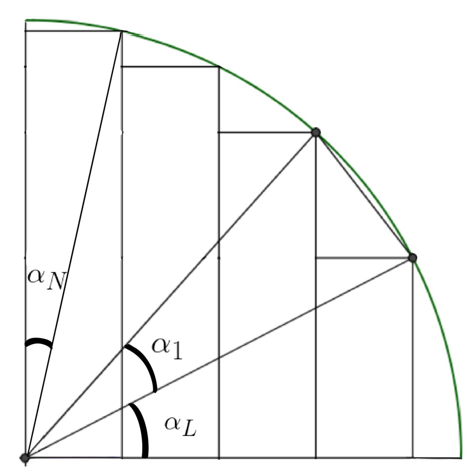
(a) Angles $\alpha$

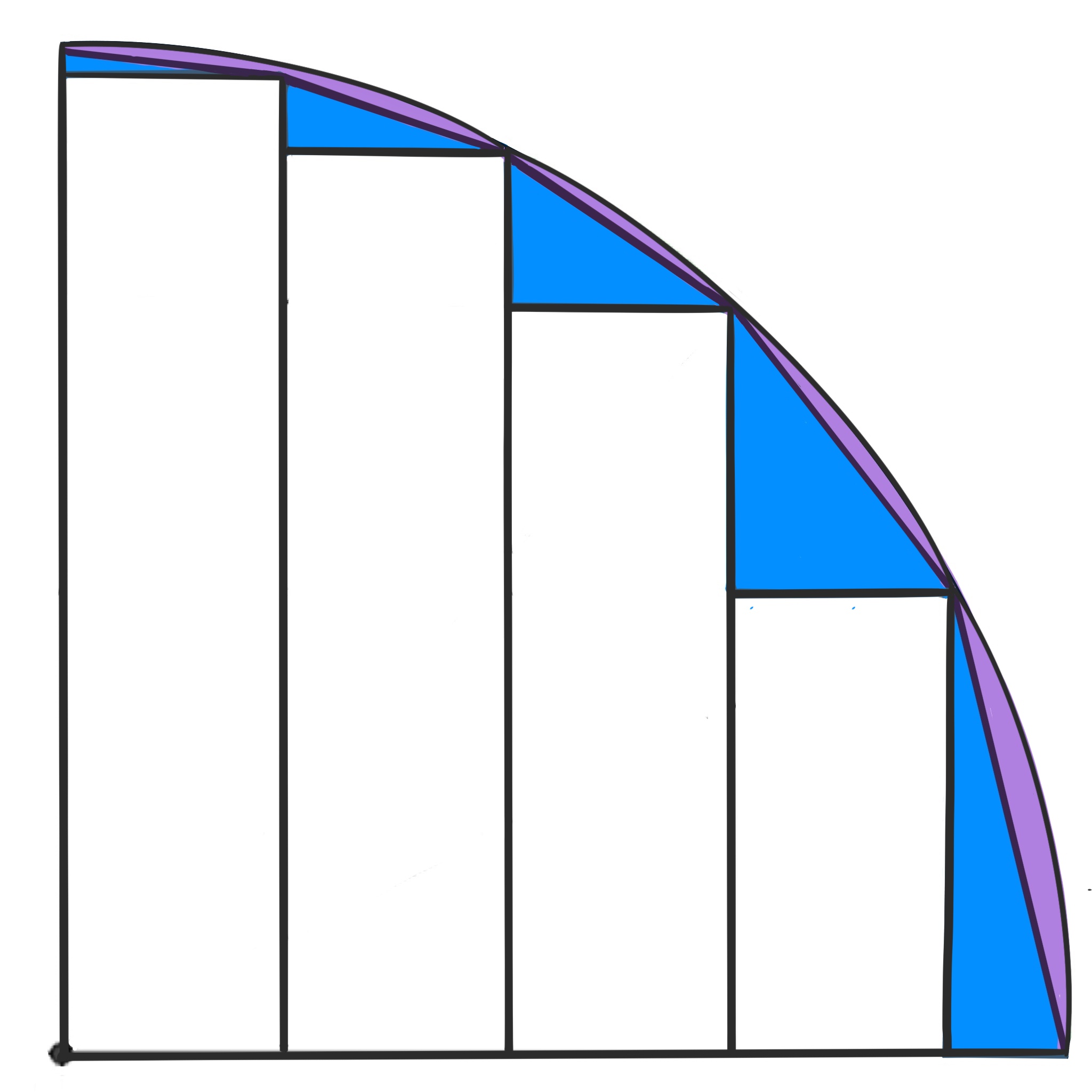
(b) Area splitting

Since the heights of the blue triangles add up to $1$, the total area $A_{1}$ is given by:

$$A_{1}=\frac{t}{2}+\frac{s-t}{2}\sqrt{1-(1-s)^{2}}=\frac{t}{2}-\frac{(t-s)\sqrt{s}}{\sqrt{2}}+\mathrm{O}(t^{5/2}).$$

Now we compute the purple area. For a sector with an angle $\alpha$, Taylor approximation dictates that the volume is given by:

$$\mathrm{Vol}({\alpha})=\frac{\alpha^{3}}{12}+\mathrm{O}(\alpha^{5}).$$

Using Taylor approximation again, note that

$$\cos\alpha=1-a\implies\mathrm{Vol}(\alpha)=\frac{\sqrt{2}a^{3/2}}{6}+\mathrm{O}(a^{5/2}).$$ (16)

Thus from the inner product,

$$\mathrm{Vol}(\alpha_{L})=\frac{\sqrt{2}s^{3/2}}{6}+\mathrm{O}(t^{5/2}).$$

Finally, we address $\mathrm{Vol}(\alpha_{1}),\ldots,\mathrm{Vol}(\alpha_{N})$. From the inner product,

$$\cos\alpha_{n+1}=(1-s-n/M)(1-s-(n+1)/M)+(1-(1-s-n/M)^{2})(1-(1-s-(n+1)/M)^{2}).$$

Setting $s_{n}:=s+n/M$, this can be rewritten as

$$\cos\alpha_{n+1}=(\sqrt{s_{n+1}}-\sqrt{s_{n}})^{2}+s_{n}s_{n+1}+2\sqrt{s_{n}s_{n+1}}\left(\sqrt{1-\frac{s_{n}}{2}}\sqrt{1-\frac{s_{n+1}}{2}}-1\right).$$

For $n\in\{0,\ldots,N-1\}$, let

$$x_{n+1}:=(\sqrt{s_{n+1}}-\sqrt{s_{n}})^{2}=\frac{1}{M}\frac{1}{(\sqrt{n+1+\delta}+\sqrt{n+\delta})^{2}}\asymp\frac{t}{n+1},$$

$$y_{n}:=s_{n}s_{n+1}+2\sqrt{s_{n}s_{n+1}}\left(\sqrt{1-\frac{s_{n}}{2}}\sqrt{1-\frac{s_{n+1}}{2}}-1\right).$$

Note that for parameters $c\in[0,1]$ and $\varepsilon$, Taylor approximation yields

$$c(c+\varepsilon)+2\sqrt{c(c+\varepsilon)}\left(\sqrt{1-\frac{c}{2}}\sqrt{1-\frac{c+\varepsilon}{2}}-1\right)=-\varepsilon^{2}\left(\frac{\sqrt{c^{2}+\varepsilon c}/4}{\sqrt{c^{2}+\varepsilon c}+c+\varepsilon/2}\right)-\varepsilon^{2}\frac{\sqrt{c^{2}+\varepsilon c}}{8(2-c)}+\mathrm{O}(\varepsilon^{3}).$$

Hence $y_{n}=\mathrm{O}(t^{2})$ and hence $y_{n}\ll x_{n}$. From(16), the volume we are to compute is given by

$$\sum_{n=1}^{N}\frac{\sqrt{2}(x_{n}+y_{n})^{3/2}}{6}+\mathrm{O}((x_{n})^{5/2})=\frac{\sqrt{2}}{6}\sum_{n=1}^{N}x_{n}^{3/2}+\frac{\sqrt{2}}{6}\sum_{n=1}^{N}\frac{3x_{n}^{2}y_{n}+3x_{n}y_{n}^{2}+y_{n}^{3}}{x_{n}^{3/2}+(x_{n}+y_{n})^{3/2}}+\mathrm{O}(t^{5/2}).$$

For parameters $x\ll y$,

$$(x+y)^{3/2}=x^{3/2}+\frac{3x^{2}y+3xy^{2}+y^{3}}{x^{3/2}+(x+y)^{3/2}}.$$

Note that

$$x_{n}-\frac{1}{4Mn}\ll\frac{1}{Mn^{2}},$$

and that

$$y_{n}-\frac{1}{4M^{2}(2-n/M)}\ll\frac{1}{M^{3}}.$$

From this one can see that

$$\frac{3x_{n}^{2}y_{n}+3x_{n}y_{n}^{2}+y_{n}^{3}}{x_{n}^{3/2}+(x_{n}+y_{n})^{3/2}}=\frac{3(x^{\prime}_{n})^{2}y^{\prime}_{n}+3x^{\prime}_{n}(y^{\prime}_{n})^{2}+(y^{\prime}_{n})^{3}}{(x^{\prime}_{n})^{3/2}+(x^{\prime}_{n}+y^{\prime}_{n})^{3/2}}+\mathrm{O}\left(\frac{1}{M^{5/2}}k^{5/2}\right),$$

where

$$x^{\prime}_{n}=\frac{1}{4Mn},y^{\prime}_{n}=\frac{1}{4M^{2}(2-n/M)}.$$

From the Euler-Maclaurin formula, we can approximate the sum for $x^{\prime}_{n},y^{\prime}_{n}$ by an integral

$$\sum_{n=1}^{N}\frac{3(x^{\prime}_{n})^{2}y^{\prime}_{n}+3x^{\prime}_{n}(y^{\prime}_{n})^{2}+(y^{\prime}_{n})^{3}}{(x^{\prime}_{n})^{3/2}+(x^{\prime}_{n}+y^{\prime}_{n})^{3/2}}=\frac{1}{8M^{2}}\int_{0}^{1}\frac{z^{2}-6z+12}{\sqrt{z}((2-z)^{3}+(2(2-z))^{3/2})}dz+\mathrm{O}(t^{5/2}).$$

The function under the integral has an explicit antiderivative given by

$$\frac{2}{\sqrt{z}}-\frac{2\sqrt{2}\sqrt{2-z}(z-1)}{\sqrt{z}(z-1)}.$$

In conclusion,

$$\sum_{n=1}^{N}\frac{3x_{n}^{2}y_{n}+3x_{n}y_{n}^{2}+y_{n}^{3}}{x_{n}^{3/2}+(x_{n}+y_{n})^{3/2}}=\frac{1}{4M^{2}}+\mathrm{O}(t^{5/2}).$$

It remains to compute $\sum_{n=1}^{N}x_{n}^{3/2}$:

$$\sum_{n}(\sqrt{s_{n+1}}-\sqrt{s_{n}})^{3} =\sum_{n=0}^{N-1}(s_{n+1})^{3/2}-3(s_{n}+1/M)\sqrt{s_{n}}+3(s_{n+1}-1/M)\sqrt{s_{n+1}}-s_{n}^{3/2}$$

$$=(-s_{0})^{3/2}+(s_{N})^{3/2}-3(s_{0}+1/M)\sqrt{s_{0}}+2(s_{N}-1/M)\sqrt{s_{N}}-\frac{6}{M}\sum_{1}^{N-1}\sqrt{s_{n}}$$

$$=-\delta^{3/2}-3(\delta+1)\sqrt{\delta}+\left((\delta+N)^{3/2}+3(\delta+N+1)\sqrt{\delta+N}-6\sum_{n=1}^{N-1}\sqrt{\delta+k}\right).$$

Now,

$$\lim_{N\to\infty}(\delta+N)^{3/2}+3(\delta+N+1)\sqrt{\delta+N}-6\sum_{n=1}^{N-1}\sqrt{\delta+k}=-6\zeta(-1/2,1+\delta),$$

∎

so

$$\sum_{n}=-\delta^{3/2}-3(\delta+1)\sqrt{\delta}-6\zeta(-1/2,1+\delta)-\sum_{N}^{\infty}(\sqrt{s_{n+1}}-\sqrt{s_{n}})^{3}.$$

Finally,

$$\sum_{N}^{\infty}(\sqrt{s_{n+1}}-\sqrt{s_{n}})^{3}=\sum_{N}^{\infty}\frac{1}{M^{3/2}}\frac{1}{(\sqrt{n+\delta}+\sqrt{n+1+\delta})^{2}}=\frac{1}{4M^{2}}+\mathrm{O}(t^{5/2})$$

by the the Euler-Maclaurin formula.

Collecting together all the terms concludes the proof.

Proof of Theorem 2.

For convenience of notation, we analyze $m(y):=M(y)/D_{2}.$

The function $m(y)$ can be re-expressed in terms of the coefficients $Q(d)$, since

$$\sum_{1\leq r\leq 2\sqrt{y}}c(r)\sqrt{y-r^{2}/4} =\sum_{\begin{subarray}{I}1\leq d\leq 2\sqrt{y}\\ d\ \square\text{-free }\end{subarray}}Q(d)\sum_{1\leq n\leq 2\sqrt{y}/d}\sqrt{y-d^{2}n^{2}/4}.$$

For a fixed value of $d$, one has:

$$\sum_{1\leq n\leq 2\sqrt{y}/d}\sqrt{y-d^{2}n^{2}/4}\leq\int_{0}^{2\sqrt{y}/d}\sqrt{y-d^{2}t^{2}/4}dt=\frac{\pi y}{2d}.$$

We let

$$F(y,d):=-\sum_{1\leq n\leq 2\sqrt{y}/d}\sqrt{y-d^{2}n^{2}/4}+\frac{\pi y}{2d}\geq 0$$

be the error term in this approximation. Then:

$$m(y) =A\sqrt{y}-\pi y-2B\sum_{\begin{subarray}{I}1\leq d\leq 2\sqrt{y}\\ d\ \square\text{-free }\end{subarray}}\left(F(d,y)Q(d)-\frac{\pi yQ(d)}{2d}\right)$$

$$=A\sqrt{y}-\pi y+y(B\pi)\sum_{\begin{subarray}{I}1\leq d\leq 2\sqrt{y}\\ d\ \square\text{-free }\end{subarray}}\frac{Q(d)}{d}-2B\sum_{\begin{subarray}{I}1\leq d\leq 2\sqrt{y}\\ d\ \square\text{-free }\end{subarray}}F(d,y)Q(d)$$

Clearly,

$$\sum_{d>2\sqrt{y}}\frac{Q(d)}{d}\ll y^{-1}.$$

Moreover, one sees from the Euler product that

$$B\pi y\sum_{\begin{subarray}{I}d\ \square\text{-free }\end{subarray}}\frac{Q(d)}{d}=\pi y,$$

and hence

$$m(y)=A\sqrt{y}-2B\sum_{\begin{subarray}{I}1\leq d\leq 2\sqrt{y}\\ d\ \square\text{-free }\end{subarray}}Q(d)F(d,y)+\mathrm{O}(1).$$

Changing variables, $F(y,d)=\sqrt{y}(1/t),t:=\frac{d}{2\sqrt{y}},$ where $\mathrm{A}(t)$ is the function from Lemma 4.1. Applying the Lemma,

$$m(y) =A\sqrt{y}-2B\sum_{\begin{subarray}{I}1\leq d\leq 2\sqrt{y}\\ d\ \square\text{-free }\end{subarray}}Q(d)\frac{2y}{d}\left(\frac{d}{4\sqrt{y}}+\frac{d^{3/2}}{2^{3/2}y^{3/4}}P(\frac{d}{2\sqrt{y}})+\mathrm{O}\left(\frac{d^{5/2}}{y^{5/4}}\right)\right)+\mathrm{O}(1)$$

$$=A\sqrt{y}-B\sqrt{y}\sum_{\begin{subarray}{I}1\leq d\leq 2\sqrt{y}\\ d\ \square\text{-free }\end{subarray}}Q(d)-y^{1/4}\sqrt{2}B\sum_{\begin{subarray}{I}1\leq d\leq 2\sqrt{y}\\ d\ \square\text{-free }\end{subarray}}Q(d)\sqrt{d}P\left(\frac{d}{2\sqrt{y}}\right)+\mathrm{O}(1).$$

Now,

$$\sum_{\begin{subarray}{I}d\ \square\text{-free }\end{subarray}}Q(d)=A/B,$$

and hence

$$m(y)=-y^{1/4}\sqrt{2}B\sum_{\begin{subarray}{I}1\leq d\leq 2\sqrt{y}\\ d\ \square\text{-free }\end{subarray}}Q(d)\sqrt{d}P\left(\frac{d}{2\sqrt{y}}\right),$$

which concludes the proof. ∎

5 Geometric Averaging

In this section we complete the proof of Theorem 3 and analyze the asymptotic behavior of the dyadic average.

Proof of Theorem 3.

Let and let $\delta_{2}$ be a parameter chosen depending on $\delta_{1}$ to satisfy the conditions of Theorem 1 with a powersaving error term. Assume further that $Y\sim X^{1-\delta_{2}}$ be a parameter chosen so $Y$ divides $Z-X$; let $X=X_{1},X_{2},\ldots,X_{G}=Z-Y$ be given by $X_{g}=X+(g-1)Y,$ where $G:=(Z-X)/Y$. From (3.3),

$$\sideset{}{{}^{\square}}{\sum}_{\begin{subarray}{I}N\in[X,Z]\end{subarray}}\sum_{f\in H^{\text{new}}(N,2)}\lambda_{f}(P)\sqrt{P}\varepsilon(f) =\sum_{g}\sideset{}{{}^{\square}}{\sum}_{\begin{subarray}{I}N\in[X_{g},X_{g+1}]\end{subarray}}\sum_{f\in H^{\text{new}}(N,2)}\lambda_{f}(P)\sqrt{P}\varepsilon(f)$$

$$=\sum_{g}\frac{X_{g}Y}{D_{k}\pi\zeta(2)}M_{k}\left(\frac{P}{X_{g}}\right)+\o\left(X^{2}.\right)$$

Since Theorem 1 gives a bound of $\mathrm{O}(k+kP/X)$ on $M$,

$$\sum_{g}X_{g}YM_{k}(P/X_{g})-\int_{X}^{Z}uM_{k}(P/u)du \ll\int_{X}^{Z}um_{k}(P/u)-(u+Y)m_{k}(p/(u+Y))u$$

$$\ll kXY(P/X+1)=o(kX^{2}).$$

Next,

$$\int_{X}^{Z}uM_{k}(p/u)du=X^{2}\int_{1}^{c}M_{k}(y/u)du.$$

Finally, from (15), we can again compute that

$$\frac{1}{\sum^{\square}_{\begin{subarray}{I}N\in[X,Z]\end{subarray}}\sum_{f\in H^{\text{new}}(N,k)}1}=\frac{24\cdot\zeta(2)\prod_{p}\left(1-\frac{1}{p^{2}+p}\right)^{-1}}{(c^{2}-1)(k-1)X^{2}}+\mathrm{O}\left(\frac{1}{kX^{12/5-\varepsilon}}\right).$$

Thus,

$$\frac{\sum^{\square}_{\begin{subarray}{I}N\in[X,Z]\end{subarray}}\sum_{f\in H^{\text{new}}(N,2)}\lambda_{f}(P)\sqrt{P}\varepsilon(f)}{\sum^{\square}_{N\in[X,Z]}\sum_{f\in H^{\text{new}}(N,2)}1} =\frac{24\zeta(2)\prod_{p}\left(1-\frac{1}{p^{2}+p}\right)^{-1}}{\pi\zeta(2)D_{k}(c^{2}-1)(k-1)}\int_{1}^{c}M_{k}(y/u)du+o_{c}(1)$$

$$=\frac{2}{(c^{2}-1)}\int_{1}^{c}M_{k}(y/u)du+o_{c}(1)$$

∎

Finally, we analyze the asymptotic behavior of the function above.

Proof of Theorem 4.

Let $f(x)=\delta_{0<x<1}\sqrt{1-x}/\sqrt{x}$. The Mellin transform of $f$ is expressible via the Beta function as

$$\tilde{f}(s) =\int_{0}^{\infty}f(x)x^{s}\frac{dx}{x}=\frac{1}{2}\int_{0}^{1}\sqrt{1-x}x^{s-1/2}\frac{dx}{x}=B\left(\frac{3}{2},s-1/2\right)$$

$$=\frac{\Gamma(s-1/2)\Gamma(3/2)}{\Gamma\left(s+1\right)}=\frac{\sqrt{\pi}}{2}\frac{\Gamma(s-1/2)}{\Gamma\left(s+1\right)}$$

By Stirling approximation,

$$\absolutevalue{\tilde{f}(\sigma+it)}\sim\absolutevalue{t}^{-3/2},$$

so we can apply Mellin inversion, which yields

$$F(x):=\sum_{r\geq 1}rc(r)f(r^{2}/x)=\sum_{r\geq 1}rc(r)\frac{1}{2\pi i}\int_{\real(s)=3}\tilde{f}(s)r(x/r^{2})^{s}ds=\frac{1}{2\pi i}\int_{\real(s)=3}L(2s-1)\tilde{f}(s)x^{s}ds,$$

where

$$L(s):=\sum_{r}c(r)r^{-s}=\prod_{p}\left(1+\left(1+\frac{p^{2}}{p^{4}-2p^{2}-p+1}\right)\frac{p^{-s}}{1-p^{-s}}\right).$$

For a function $\Phi:(0,\infty)\to\mathbb{R}$ of compact support, let

$$F_{\Phi}(x):=\left(\int_{0}^{\infty}F\left(\frac{x}{u}\right)\Phi(u)u^{2}\frac{du}{u}\right)/\tilde{\Phi}(2).$$

By definition,

$$(D_{2}B)\cdot F_{\Phi}(x)=\left(\int_{0}^{\infty}\sum_{1\leq r\leq x}c(r)\sqrt{(x/u)-r^{2}}\Phi(u)u^{2}\frac{du}{u}\right)/\int_{0}^{\infty}\Phi(u)u^{2}\frac{du}{u}.$$

Then by Mellin inversion,

$$F_{\Phi}(x)=\frac{1}{2\pi i}\int_{\real(s)=3}L(2s-1)\tilde{f}(s)\tilde{\Phi}(s+2)x^{s}ds.$$ (17)

Now, we can further simplify $L$ as:

$$L(s)=\frac{\zeta(s)\zeta(s+2)}{\zeta(2s+4)}\prod_{p}\left(1+\frac{-1+p+2p^{2}}{(1-p-2p^{2}+p^{4})(1+p^{2+s})}\right).$$

The Euler product part in the expression above evaluated at $2s-1$ converges uniformly for $s>\sigma$ for any $\sigma>-1$, so it is analytic and uniformly bounded in this region. The Mellin transform $\tilde{\Phi}$ is entire because of the support assumption, and if $\Phi$ is smooth, the decay of $\Phi$ in the $t$ aspect allows us to shift the contour in (17) to the line $\real(s)=-1/2$. The poles at $1$ and $1/2$ cancel our exactly the contribution of the $\pi y$ and $A\sqrt{y}$ terms in $M_{\Phi}(y)$. Finally, the residue at $0$ is

$$\frac{\sqrt{\pi}}{2}\frac{\Gamma\left(\frac{-1}{2}\right)}{\Gamma(1)}\frac{\zeta(-1)}{\zeta(2)}\prod_{p}\left(1+\frac{-1+p+2p^{2}}{(1-p-2p^{2}+p^{4})(1+p)}\right)=1/BD_{2}.$$

∎

6 Arithmetic Functions

In this section, we collect auxiliary definitions, notation, and lemmas.

Definition 6.1.

Let $\varphi(m)$ be Euler’s function and ${\psi}(m)$ be the Dedekind Psi function. Let

$$\eta(m):=\frac{m}{\psi(m)}=\prod_{p|m}\frac{p}{p+1}.$$

For any $r,m\in\mathbb{N}$ and a prime $P$, let

$$\theta_{r}(m):=\sum_{a\hskip 1.4457pt\mathrm{mod}\hskip 1.4457ptm}\left(\frac{a}{m}\right)\left(\frac{ar^{2}-4P}{m}\right).$$

We let

$$\widetilde{\Phi}_{r,d}(g):=\sum_{\begin{subarray}{I}a\hskip 1.4457pt\mathrm{mod}\hskip 1.4457ptd^{2}g\\ a\hskip 1.4457pt\mathrm{mod}\hskip 1.4457ptd^{2}\in\mathcal{R}_{r,d}\end{subarray}}\left(\frac{a}{g}\right)\left(\frac{(r^{2}a-4P)/d^{2}}{g}\right)$$

for $d,g,r\in\mathbb{N}$.

Lemma 6.2.

For any modulus $m$ and a prime $P\neq 2$ with $(m,P)=1$, $\theta_{r}(m)$ is a multiplicative function of $m$. For odd $r$, it is given as follows. For a prime $p$ with $(p,2k)=1$,

$$\theta_{r}(p^{\alpha})=-p^{\alpha-1}\text{ for }\alpha\text{ odd};\ \ \theta_{r}(p^{\alpha})=p^{\alpha-1}(p-2)\text{ for }\alpha\text{ even}.$$

For $p|r,$

$$\theta_{r}(p^{\alpha})=0\text{ for }\alpha\text{ odd};\ \ \theta_{r}(p^{\alpha})=p^{\alpha-1}(p-1)\text{ for }\alpha\text{ even};$$

For $p=2$,

$$\theta_{r}(2^{\alpha}):=(-1)^{\alpha}2^{\alpha-1}.$$

For even $r$,

$$\theta_{r}(2^{\alpha})=0$$

for any $\alpha\geq 1$; for an odd prime $p$, $\theta_{r}(p^{\alpha})=\theta_{r^{\prime}}(p^{\alpha}),$ where $r^{\prime}$ is the odd part of $r$.

Proof.

∎

Lemma 6.3.

Let $d,g,r\in\mathbb{N}$ be such that $g|d^{\infty}$. Then:

$$\widetilde{\varphi}_{r,d}(g)=\begin{cases}\varphi(g)\delta_{g=\square}&\text{ if }2\nmid d\\ \varphi(g)\delta_{g=\square}&\text{ if }2||d,2\nmid n\\ 0&\text{ if }2||d,2|n,2||r\\ 2\varphi(g)\delta_{g=\square}&\text{ if }2||d,2|n,4|r\\ 2\varphi(g)\delta_{g=\square}&\text{ if }4|d\end{cases}.$$

If $(d,r)$ is non-admissible, $\widetilde{\varphi}_{r,d}(g)=0$, so assume it is an admissible pair. Let $r$ be an integer that reduces to an element of $\mathcal{R}_{r,d}$ modulo $d^{2}$, let $s:=(r^{2}r-4P)/d^{2}$, and let $g=:2^{\alpha}h$, where $(h,2)=1$. Since $h$ is odd, $\left(\frac{\cdot}{h}\right)$ is a character modulo $\mathrm{rad}\ h$, and since $\mathrm{rad}\ h|d^{2}$, we have

$$\sum_{\begin{subarray}{I}a\hskip 1.4457pt\mathrm{mod}\hskip 1.4457ptd^{2}g\\ a\equiv r\hskip 1.4457pt\mathrm{mod}\hskip 1.4457ptd^{2}\end{subarray}}\left(\frac{a}{g}\right)\left(\frac{(r^{2}a-4P)/d^{2}}{g}\right) =\sum_{\begin{subarray}{I}t=1\end{subarray}}^{g}\left(\frac{r+td^{2}}{g}\right)\left(\frac{s+tr^{2}}{g}\right)$$

$$=\sum_{t\hskip 1.4457pt\mathrm{mod}\hskip 1.4457pth}\left(\frac{r}{h}\right)\left(\frac{s+tr^{2}}{h}\right)\sum_{t\hskip 1.4457pt\mathrm{mod}\hskip 1.4457pt2^{\alpha}}\left(\frac{r+td^{2}}{2^{\alpha}}\right)\left(\frac{s+tr^{2}}{2^{\alpha}}\right)$$

$$=\delta_{h=\square}\varphi(h)\sum_{t\hskip 1.4457pt\mathrm{mod}\hskip 1.4457pt2^{\alpha}}\left(\frac{r+td^{2}}{2^{\alpha}}\right)\left(\frac{s+tr^{2}}{2^{\alpha}}\right).$$

where in the last step we used that $(h,k)=1$ because $(r,d)\leq 2$ by assumption. We compute

$$\star:=\sum_{t\hskip 1.4457pt\mathrm{mod}\hskip 1.4457pt2^{\alpha}}\left(\frac{r+td^{2}}{2^{\alpha}}\right)\left(\frac{s+tr^{2}}{2^{\alpha}}\right)$$

case by case.

1. If $\alpha=0$, i.e., $2\nmid g$, then $\star=1$, so $\widetilde{\varphi}(g)=2\delta_{g=\square}\varphi(g)$ if $4|d$ and $2\delta_{g=\square}\varphi(g)$ otherwise;

   If $2|g$ (and hence $2|d$ and $2|r$ from admissibility), then $r$ is odd since $(r,d)=1$ for all $r\in\mathcal{R}_{d,r}$, and:

2. If $2||r,2||d$, then $s$ is even and $\star=0$.

3. If $4|r$ and $2||d$, $\mathcal{R}_{r,d}$ has one element and the corresponding $s$ is odd, and so using that

   $$\left(\frac{x+4}{2}\right)=-\left(\frac{x}{2}\right),$$

   we see

   $$\star=\sum_{t\hskip 1.4457pt\mathrm{mod}\hskip 1.4457pt2^{\alpha}}\left(\frac{z+4t}{2^{\alpha}}\right)\left(\frac{z^{\prime}}{2^{\alpha}}\right)=\delta_{2|\alpha}2^{\alpha};$$

4. if $4|d$ and $2||r$, there’s exactly one choice of $r\in\mathcal{R}_{r,d}$ for which $s$ is odd; for this choice of $r$, once again $\star=\delta_{2^{\alpha}=\square}2^{\alpha};$ for the other choice of $r$, $s$ is even and $\star=0$.

Combining all the cases, we get the statement of the lemma.

Theorem 6.4 (Hooley, [5]).

: Let $(a,m)=1$.

$$\sum_{\begin{subarray}{I}N=X\\ N=a\hskip 1.4457pt\mathrm{mod}\hskip 1.4457ptm\end{subarray}}^{X+Y}\mu^{2}(N)=\frac{Y}{\zeta(2)}\frac{\eta(m)}{\varphi(m)}+O(\sqrt{X/m}+m^{1/2+\varepsilon}).$$

Lemma 6.5.

Let $K$ be a cut-off parameter and let $P\neq 2$ be a prime. Let

$$A:=\prod_{p}(1+\frac{p}{(p+1)^{2}(p-1)});$$

1. $$\sum_{\begin{subarray}{I}m\text{ odd }\\ (P,m)=1\end{subarray}}^{K}\frac{1}{m^{2}}\eta(m)=\prod_{p\neq 2,P}\left(1+\frac{p}{(p+1)^{2}(p-1)}\right)+\mathrm{O}\left(\frac{1}{K}\right)=\frac{9A}{11}+\mathrm{O}\left(\frac{1}{P^{2}}+\frac{1}{K}\right);$$

2. $$\sum_{\begin{subarray}{I}m:(P,m)=1\end{subarray}}^{K}\ \frac{1}{m^{2}}\eta(2m)=\frac{2}{3}\sum_{k\geq 0}2^{-k}\prod_{p\neq 2,P}\left(1+\frac{p}{(p+1)^{2}(p-1)}\right)=\frac{8A}{11}+\mathrm{O}\left(\frac{1}{P^{2}}+\frac{1}{K}\right);$$

Lemma 6.6.

Let $\mathcal{T}_{r}\subseteq\mathbb{N}^{3}$ denote the set of triples $(m,d,g)$ such that $(d,r)$ is admissible, $(m,d)=1$, and $g|d^{\infty}.$

$$\Theta_{r}(m,d,g):=\frac{\eta(d^{2}mg)}{\varphi(d^{2}mg)}\frac{\theta_{r}(m)\widetilde{\varphi}(g)}{mgd}.$$

Then $\sum_{\mathcal{T}_{r}}\Theta_{r}(m,d,g)$ is absolutely convergent and equal to

$$B\cdot c(r):=\prod_{p}\frac{p^{4}-2p^{2}-p+1}{(p^{2}-1)^{2}}\prod_{p|r}\left(1+\frac{p^{2}}{p^{4}-2p^{2}-p+1}\right).$$

Moreover,

$$\sum_{\begin{subarray}{I}(m,d,g)\in\mathcal{T}_{r}\\ mg\leq Z^{\prime},d\leq Z\end{subarray}}\Theta_{r}(m,d,g)-Bc(r)\ll Z^{-2}+(Z^{\prime})^{-1/5}.$$

Proof.

Define $E:=\prod_{p}\left(1+\frac{p}{(p^{2}-1)^{2}}\right),E(k):=\prod_{p|r}\left(1+\frac{p}{(p^{2}-1)^{2}}\right),$ $G:=\prod_{p}\left(1-\frac{2p}{(p^{2}-1)^{2}+p}\right),G(k):=\prod_{p|r}\left(1-\frac{2p}{(p^{2}-1)^{2}+p}\right),$ and $F(k):=\prod_{p|r}\left(1+\frac{p(p-1)}{(p^{2}-1)^{2}}\right).$ It is easy to verify that

$$Bc(r)=\frac{EGF(k)}{E(k)G(k)}.$$

Next, since $g|d^{\infty}$ and $(m,d)=1$, we have $\{p|md^{2}g\}=\{p|d\}\sqcup\{p|m\},$ so

$$\Theta_{r}(m,d,g)=\frac{1}{d^{3}\prod_{p|d}(1-1/p^{2})}\frac{\theta_{r}(m)}{m^{2}\prod_{p|m}(1-1/p^{2})}\frac{\widetilde{\varphi}(g)}{g^{2}}.$$

We begin by establishing absolute convergence. For fixed $m,d$, the sum

$$\sideset{}{{}^{g}}{\sum}:=\sum_{g|d^{\infty}}\frac{\widetilde{\varphi}(g)}{g^{2}}$$

over $g$’s appearing in $\mathcal{T}_{r}$ for these $m$ and $d$ is upper bounded by

$$\sum_{\begin{subarray}{I}g|d^{\infty}\\ g=\square\end{subarray}}\frac{2\varphi(g)}{g^{2}}=2\prod_{p|d}\left(1+\sum_{k\geq 1}\frac{p-1}{p}\frac{1}{p^{2k}}\right)=2\prod_{p|d}\left(1+\frac{1}{p(p+1)}\right)\ll\prod_{p}(1+1/p^{2})\leq\prod_{p}1/(1-1/p^{2})=\zeta(2),$$

so is uniformly bounded.

Now fix $d$. Any number $r$ can be written uniquely as $a^{2}\cdot b\cdot 2^{c}$, where $b$ is square-free and $a,b$ odd. From the definition of $\theta_{r}$,

$$\absolutevalue{\theta_{r}(a^{2}\cdot b\cdot 2^{c})}\leq a^{2}\cdot 2^{c}.$$

In particular, using that $\prod_{p|m}(1-1/p^{2})\gg 1$,

$$\sum_{(m,d)=1}\frac{\theta_{r}(m)}{m^{2}\prod_{p|m}(1-1/p^{2})}\ll\sum_{m\in\mathbb{N}}\absolutevalue{\theta_{r}(m)}/m^{2}\ll\left(\sum_{c\in\mathbb{N}}1/2^{c}\right)\left(\sum_{a\in\mathbb{N}}1/a^{2}\right)\left(\sum_{b\ \square\text{ - free}}1/b^{2}\right)\ll 1.$$

Finally,

$$\sum_{d\in\mathbb{N}}\frac{1}{d^{3}\prod_{p|d}(1-1/p^{2})}\ll 1,$$

so indeed, the series $\sum_{\mathcal{T}_{r}}\Theta_{r}(m,d,g)$ converges absolutely.

Next, we compute $\sideset{}{{}^{g}}{\sum}$ case by case from the definition.

• When $2\nmid d$, $\widetilde{\varphi}(g)=\delta_{g=\square}\varphi(g),$ and

  $$\sideset{}{{}^{g}}{\sum}=\sum_{\begin{subarray}{I}g|d^{\infty}\\ g=\square\end{subarray}}\frac{\varphi(g)}{g^{2}}=\prod_{p|d}\left(1+\frac{1}{p(p+1)}\right);$$

• When $2||d$ and $2||r$, $\widetilde{\varphi}(g)=\delta_{g=\square}\varphi(g)$ for odd $g$ and $0$ for even $g$, so

  $$\sideset{}{{}^{g}}{\sum}=\sum_{\begin{subarray}{I}g|d^{\infty}\\ g=\square\\ 2\nmid g\end{subarray}}\frac{\varphi(g)}{g^{2}}=\prod_{p|d_{o}}\left(1+\frac{1}{p(p+1)}\right)$$

  where $d_{o}$ is the odd part of $d$;

• When $2||d$ and $4|r$, then $\widetilde{\varphi}(g)=\delta_{g=\square}\varphi(g)$ for $g$ odd and $\widetilde{\varphi}(g)=2\delta_{g=\square}\varphi(g)$ for $g$ even, so

  $$\sideset{}{{}^{g}}{\sum}=\sum_{\begin{subarray}{I}g|d_{0}^{\infty}\\ g=\square\end{subarray}}\frac{\varphi(g)}{g^{2}}+2\sum_{\begin{subarray}{I}g|d^{\infty}\\ g=\square\\ 2|g\end{subarray}}\frac{\varphi(g)}{g^{2}}=\frac{4}{3}\prod_{p|d_{o}}\left(1+\frac{1}{p(p+1)}\right);$$

• When $4|d$ and $2||r$, then $\widetilde{\varphi}(g)=2\delta_{g=\square}\varphi(g)$, so

  $$\sideset{}{{}^{g}}{\sum}=2\prod_{p|d}\left(1+\frac{1}{p(p+1)}\right)=\frac{7}{3}\prod_{p|d_{o}}\left(1+\frac{1}{p(p+1)}\right);$$

We can now compute the desired sum by expressing it as an Euler product.

Suppose first that $r$ is odd, so $(r,d)$ is admissible if and only if $d$ is odd and $(r,d)=1$. Then

$$\sum_{\mathcal{T}_{r}}\Theta_{r}(m,d,g) =\sum_{\begin{subarray}{I}d\text{ odd}\\ (d,r)=1\end{subarray}}\sum_{(m,d)=1}\frac{\prod_{p|d}(1+1/p(p+1))}{d^{3}\prod_{p|d}(1-1/p^{2})}\frac{\theta_{r}(m)}{m^{2}\prod_{p|m}(1-1/p^{2})}$$

$$=\sum_{m}\frac{\theta_{r}(m)}{m^{2}\prod_{p|m}(1-1/p^{2})}\sum_{(d,2mr)=1}\frac{1}{d^{3}}\prod_{p|d}\frac{p(1+p+p^{2})}{(p-1)(p+1)^{2}}.$$

The inner sum can be expressed as the Euler product

$$\prod_{p\nmid 2mr}\left(1+\sum_{k\geq 1}\frac{1}{p^{3k}}\frac{p(1+p+p^{2})}{(p-1)(p+1)^{2}}\right)=\prod_{p\nmid 2mr}\left(1+\frac{p}{(p^{2}-1)^{2}}\right)=\prod_{p}\left(1+\frac{p}{(p^{2}-1)^{2}}\right)/\prod_{p|2mr}\left(1+\frac{p}{(p^{2}-1)^{2}}\right)$$

so

$$\sum_{\mathcal{T}_{r}}\Theta_{r}(m,d,g)=\frac{E}{E(k)}\cdot\sum_{m}\frac{\theta_{r}(m)}{m^{2}}\prod_{p|m}(1-1/p^{2})^{-1}\prod_{p|2m,p\nmid k}(1+p/(p^{2}-1)^{2})^{-1}.$$

This sum over $m$ can itself be expressed as an Euler product. The $p\neq 2$, $p\nmid r$ part of the product is

$$\prod_{p\nmid 2k}\left(1+\frac{1}{(1-1/p^{2})(1+p/(p^{2}-1)^{2})}\left(\sum_{\alpha\geq 0}\frac{\theta_{r}(p^{2\alpha+1})}{p^{4\alpha+2}}+\sum_{\alpha\geq 0}\frac{\theta(p^{2\alpha+2})}{p^{4\alpha+4}}\right)\right)$$

$$= \prod_{p\nmid 2k}\left(1+\frac{1}{(p^{2}-1)(1+p/(p^{2}-1)^{2})}\left(-\sum_{\alpha\geq 0}\frac{1}{p^{2\alpha}}+\sum_{\alpha\geq 0}\frac{(p-2)}{p^{2\alpha+1}}\right)\right)$$

$$= \prod_{p\nmid 2k}\left(1-\frac{2p}{(p^{2}-1)^{2}+p}\right)=\frac{G}{G(2k)}.$$

The $p|r$ factors are

$$\prod_{p|r}\left(1+\frac{1}{1-1/p^{2}}\left(\sum_{\alpha\geq 0}\frac{\theta_{r}(p^{2\alpha+1})}{p^{4\alpha+2}}+\sum_{\alpha\geq 0}\frac{\theta(p^{2\alpha+2})}{p^{4\alpha+4}}\right)\right) =\prod_{p|r}\left(1+\frac{1}{p^{2}-1}\sum_{\alpha\geq 0}\frac{p-1}{p^{2\alpha+1}}\right)$$

$$=\prod_{p|r}\left(1+\frac{p(p-1)}{(p^{2}-1)^{2}}\right)=F(k).$$

The Euler factor at $2$ is

$$\frac{1}{1+2/(2^{2}-1)^{2}}\left(1+\sum_{\alpha\geq 1}\left(1-\frac{1}{2^{2}}\right)^{-1}\frac{(-1)^{\alpha}2^{\alpha-1}}{2^{2\alpha}}\right)=\frac{9}{11}\left(1+\frac{1}{2}\frac{4}{3}\sum_{\alpha\geq 1}(-1/2)^{\alpha}\right)=\frac{7}{11}=G(2).$$

All the Euler factors together add up to $Bc(r)$.

Now we estimate the tail, namely, the contribution of terms with $d>Z$ or $mg>W$. As noted above, for $d$ fixed,

$$\sum_{(m,d)=1}\sum_{g|d^{\infty},g=\square}\frac{\theta_{r}(m)}{m^{2}\prod_{p|m}(1-1/p^{2})}\frac{\varphi(g)}{g^{2}}$$

is uniformly bounded; hence,

$$\sum_{(m,d,g)\in\mathcal{T}_{r}:d\geq Z}\Theta_{r}(m,d,g)\ll\sum_{d\geq Z}\frac{1}{d^{3}\prod_{p|d}(1-1/p^{2})}\ll Z^{-2}.$$ (18)

For a given $g$, the contribution of summands with that $g$ is

$$\frac{\varphi(g)}{g^{2}}\sum_{\begin{subarray}{I}m,d\\ (m,d)=1\\ d\text{ odd}\\ g|d^{\infty}\end{subarray}}\frac{1/d^{3}}{\prod_{p|d}(1-1/p^{2})}\frac{\theta_{r}(m)/m^{2}}{\prod_{p|m}(1-1/p^{2})}\leq\frac{\varphi(g)}{g^{2}}\sum_{\begin{subarray}{I}m,d\\ (m,d)=1\\ d\text{ odd}\end{subarray}}\frac{1/d^{2}}{\prod_{p|d}(1-1/p^{2})}\frac{|\theta_{r}(m)|/m^{2}}{\prod_{p|m}(1-1/p^{2})}\ll\frac{\varphi(g)}{g^{2}}.$$

Here we used that $\sum_{\begin{subarray}{I}m,d\\ (m,d)=1\\ d\text{ odd}\end{subarray}}\frac{1/d^{2}}{\prod_{p|d}(1-1/p^{2})}\frac{|\theta_{r}(m)|/m^{2}}{\prod_{p|m}(1-1/p^{2})}$ converges since these are terms of the original sum corresponding to $g=1$. From this,

$$\sum_{(m,d,g)\in\mathcal{T}_{r}:g\geq W}\Theta_{r}(m,d,g)\ll\sum_{t>\sqrt{W}}\frac{1}{t^{2}}\ll W^{-1/2}.$$ (19)

Finally, the terms in the sum corresponding to elements of $\mathcal{T}_{r}$ with a fixed $m$ are

$$\frac{\theta_{r}(m)/m^{2}}{\prod_{p|m}(1-1/p^{2})}\sum_{\begin{subarray}{I}g,d\\ (m,d)=1\\ d\text{ odd}\\ g|d^{\infty}\end{subarray}}\frac{\varphi(g)}{g^{2}}\frac{1/d^{3}}{\prod_{p|d}(1-1/p^{2})}\leq\frac{\theta_{r}(m)/m^{2}}{\prod_{p|m}(1-1/p^{2})}\sum_{\begin{subarray}{I}g,d\\ d\text{ odd}\\ g|d^{\infty}\end{subarray}}\frac{\varphi(g)}{g^{2}}\frac{1/d^{3}}{\prod_{p|d}(1-1/p^{2})}\ll\frac{\theta_{r}(m)/m^{2}}{\prod_{p|m}(1-1/p^{2})},$$

where again, $\sum_{\begin{subarray}{I}g,d\\ d\text{ odd}\\ g|d^{\infty}\end{subarray}}\frac{\varphi(g)}{g^{2}}\frac{1/d^{3}}{\prod_{p|d}(1-1/p^{2})}$ converges since these are the $m=1$ terms in the original sum. Thus,

$$\sum_{(m,d,g)\in\mathcal{T}_{r}:m\geq V}\Theta_{r}(m,d,g)\ll\sum_{m\geq V}|\theta_{r}(m)|/m^{2}.$$

Recall that for $m=a^{2}\cdot b\cdot 2^{c}$ for $b$ square-free, $a,b$ odd, one has $\theta_{r}(m)/m^{2}\ll\frac{1}{a^{2}b^{2}2^{c}}.$ Hence

$$\sum_{m\geq V}|\theta_{r}(m)|/m^{2}\leq\sum_{c\geq 1}\frac{1}{2^{c}}\sum_{\begin{subarray}{I}m=a^{2}b\text{ odd }\\ m\geq V/2^{c}\end{subarray}}|\theta_{r}(m)|/m^{2} \ll\sum_{c\geq 1}\frac{1}{2^{c}}\Big{(}\sum_{a>(V/2^{c})^{1/3}}\sum_{b}\frac{1}{a^{2}b^{2}}+\sum_{b>(V/2^{c})^{1/3}}\sum_{a}\frac{1}{a^{2}b^{2}}\Big{)}$$

$$\ll\sum_{c}\frac{1}{2^{c}}\frac{2^{c/3}}{V^{1/3}}\ll V^{-1/3}.$$ (20)

Finally, let $Z^{\prime}=VW$, where $V=Z^{3/5}$, $V=Z^{2/5}$. Then $gm>Z^{\prime}$ implies that at least one of $g>W$ or $m>V$ holds, so putting together (18), (19), and (6),

$$\sum_{\begin{subarray}{I}(m,d,g)\in\mathcal{T}_{r}\\ mg\geq Z^{\prime}\text{ or }d\geq Z\end{subarray}}\Theta_{r}(m,d,g)\ll Z^{-2}+(Z^{\prime})^{-1/5}.$$

Next, suppose $r$ is even, let $r_{o}$ the odd part of $r$.

$$\sum_{\mathcal{T}_{r}}\Theta_{r}(m,d,g) =\sum_{\begin{subarray}{I}d\text{ odd }\\ (d,k_{o})=1\end{subarray}}\sum_{(m,2d)=1}\frac{\prod_{p|d_{o}}(1+1/p(p+1))}{d^{3}\prod_{p|d}(1-1/p^{2})}\frac{\theta_{k_{o}}(m)}{m^{2}\prod_{p|m}(1-1/p^{2})}$$

$$+\sum_{\begin{subarray}{I}2||d\\ (d,k_{o})=1\end{subarray}}\sum_{(m,d)=1}\frac{\prod_{p|d_{o}}(1+1/p(p+1))}{d^{3}\prod_{p|d}(1-1/p^{2})}\frac{\theta_{k_{o}}(m)}{m^{2}\prod_{p|m}(1-1/p^{2})}$$

$$+\frac{7}{3}\sum_{\begin{subarray}{I}4|d\\ (d,k_{o})=1\end{subarray}}\sum_{(m,d)=1}\frac{\prod_{p|d_{o}}(1+1/p(p+1))}{d^{3}\prod_{p|d}(1-1/p^{2})}\frac{\theta_{k_{o}}(m)}{m^{2}\prod_{p|m}(1-1/p^{2})}$$

$$=:I+II+(7/3)III.$$

We compute the three summands $I,II,$ and $III$, separately.

Observe that for $m$ odd and $\alpha\geq 1$,

$$\frac{\theta_{k_{o}}(2^{\alpha}m)}{2^{2\alpha}m^{2}\prod_{p|2m}(1-1/p^{2})}=\frac{1}{2^{2\alpha}}\frac{1}{1-1/4}(-1)^{\alpha}2^{\alpha-1}\frac{\theta_{k_{o}}(m)}{m^{2}\prod_{p|m}(1-1/p^{2})}=\frac{2\cdot(-1)^{\alpha}}{3\cdot 2^{\alpha}}\frac{\theta_{k_{o}}(m)}{m^{2}\prod_{p|m}(1-1/p^{2})}.$$

Thus

$$I=\sum_{\begin{subarray}{I}d\text{ odd }\\ (d,k_{o})=1\end{subarray}}\sum_{(m,d)=1}\frac{\prod_{p|d}(1+1/p(p+1))}{d^{3}\prod_{p|d}(1-1/p^{2})}\frac{\theta_{k_{o}}(m)}{m^{2}\prod_{p|m}(1-1/p^{2})}\left(1+\sum_{\alpha\geq 1}\frac{2\cdot(-1)^{\alpha}}{3\cdot 2^{\alpha}}\right)^{-1}=\frac{9}{7}\sum_{\mathcal{T}_{k_{o}}}\Theta_{k_{o}}(m,d,g).$$

For $II$, we can rewrite

$$II=\sum_{\begin{subarray}{I}d_{o}\text{ odd }\\ (d,k_{o})=1\end{subarray}}\frac{1}{8(1-1/4)}\frac{\prod_{p|}(1+1/p(p+1))}{d^{3}\prod_{p|d}(1-1/p^{2})}\sum_{(m,2d_{o})=1}\frac{\theta_{k_{o}}(m)}{m^{2}\prod_{p|m}(1-1/p^{2})}=\sum_{\begin{subarray}{I}d\text{ odd }\\ (d,k_{o})=1\end{subarray}}\frac{9}{7}\frac{1}{6}\sum_{\mathcal{T}_{k_{o}}}\Theta_{k_{o}}(m,d,g).$$

Finally,

$$III=\sum_{\alpha\geq 2}\sum_{\begin{subarray}{I}d_{o}\text{ odd }\\ (d,k_{o})=1\end{subarray}}\frac{1}{8^{\alpha}(1-1/4)}\frac{\prod_{p|d}(1+1/p(p+1))}{d^{3}\prod_{p|d}(1-1/p^{2})}\sum_{(m,2d)=1}\frac{\theta_{k_{o}}(m)}{m^{2}\prod_{p|m}(1-1/p^{2})}=\frac{9}{7}\frac{1}{6\cdot 7}\sum_{\mathcal{T}_{k_{o}}}\Theta_{k_{o}}(m,d,g).$$

In summary,

$$\frac{\theta_{k_{o}}(2^{\alpha}m)}{2^{2\alpha}m^{2}\prod_{p|2m}(1-1/p^{2})}=\frac{11}{9}\left(1+\frac{1}{6}+\frac{1}{6\cdot 7}\frac{7}{3}\right)\sum_{\mathcal{T}_{k_{o}}}\Theta_{k_{o}}(m,d,g)=\frac{11}{7}\sum_{\mathcal{T}_{k_{o}}}\Theta_{k_{o}}(m,d,g).$$

It remains to notice that $c(r)=11/7c(k_{o})$.

Finally, we address the case $4|r$:

$$\sum_{\mathcal{T}_{r}}\Theta_{r}(m,d,g) =\sum_{\begin{subarray}{I}d\text{ odd }\\ (d,k_{o})=1\end{subarray}}\sum_{(m,2d)=1}\frac{\prod_{p|d_{o}}(1+1/p(p+1))}{d^{3}\prod_{p|d}(1-1/p^{2})}\frac{\theta_{k_{o}}(m)}{m^{2}\prod_{p|m}(1-1/p^{2})}$$

$$+\frac{4}{3}\sum_{\begin{subarray}{I}2||d\\ (d,k_{o})=1\end{subarray}}\sum_{(m,d)=1}\frac{\prod_{p|d_{o}}(1+1/p(p+1))}{d^{3}\prod_{p|d}(1-1/p^{2})}\frac{\theta_{k_{o}}(m)}{m^{2}\prod_{p|m}(1-1/p^{2})}.$$

Since the first summand matches $I=\frac{9}{7}\cdot c(k_{o})$; the second is equal to $\frac{4}{3}\cdot II=\frac{4}{3}\frac{1}{6}\frac{9}{7}\cdot c(k_{o})=\frac{2}{7}c(k_{o}),$ and we get the desired answer once again.

The error term analysis for $r$ even matches that of odd $r$.

∎

Lemma 6.7.

Let $m\in\mathbb{N}$, and let $\chi$ be a real character modulo $m$ coming from a primitive character modulo $m_{0}$. Let

$$\sigma_{\chi}(Z):=\sum_{\begin{subarray}{I}N\leq Z\end{subarray}}\mu^{2}(N)\chi(N).$$

Then:

$$\sigma_{\chi}(Z)=\frac{Z}{\zeta(2)}\prod_{p|m}\frac{p}{p+1}+O_{\varepsilon}\left(Z^{3/5+\varepsilon}m^{\varepsilon}\right)=Z\cdot\frac{\eta(m)}{\zeta(2)}+O_{\varepsilon}\left(Z^{3/5+\varepsilon}m^{\varepsilon}\right)$$

if $\chi$ is the principal character, and

$$\sigma_{\chi}(Z)=O_{\varepsilon}\left(Z^{3/5+\varepsilon}m^{\varepsilon}m_{0}^{1/5+\varepsilon}\right)$$

if $\chi$ is non-principal.

Proof.

Consider the associated Dirichlet series

$$\mathcal{L}_{\chi}(s):=\sum_{n}\mu^{2}(n)\chi(n)n^{-s}=\prod_{p}\left(1+\chi(p)p^{-s}\right)=\frac{L(s,\chi)}{L(2s,\chi^{2})},$$

where $L(s,\chi)$ is the Dirichlet series associated to $\chi$. By Perron’s formula (see [15], p. 70), choosing $Z$ near a half-integer, we have

$$\sum_{N\leq Z}\mu^{2}(N)\chi(N)=\frac{1}{2\pi i}\int_{1+\varepsilon-iT}^{1+\varepsilon+iT}\mathcal{L}_{\chi}(s)\frac{Z^{s}}{s}ds+\mathrm{O}_{\varepsilon}\left(\frac{Z^{1+\varepsilon}}{T}\right)$$

Suppose first that $\chi$ is the principal character. Then we have

$$\mathcal{L}_{\chi}(s)=\frac{\zeta(s)}{\zeta(2s)}\prod_{p\mid m}\frac{1}{1+p^{-s}},$$

and shifting the integral to the left of the line $\real(s)=1$ picks up the pole of $\zeta(s)$ at $s=1$. We have:

$$\mathrm{Res}_{s=1}\mathcal{L}_{\chi}(s) =\frac{1}{\zeta(2)}\prod_{p|m}\frac{1}{1+1/p}$$

Since there are no other poles to the right of the line $1/2$, shifting the contour to the line $\real(s)=1/2+\varepsilon,$

$$\sum_{\begin{subarray}{I}N\leq Z\end{subarray}}\mu^{2}(N)\chi(N) =\frac{Z}{\zeta(2)}\prod_{p|m}\frac{p}{p+1}+\frac{1}{2\pi i}\int_{\mathcal{C}}\mathcal{L}_{\chi}(s)\frac{Z^{s}}{s}ds+\mathrm{O}_{\varepsilon}\left(\frac{Z^{1+\varepsilon}}{T}\right),$$

where the integration contour $\mathcal{C}$ as shown in Figure 6(a). Similarly, if $\chi$ is non-principal, there are no poles inside of the contour, and

$$\sum_{\begin{subarray}{I}N\leq Z\end{subarray}}\mu^{2}(N)\chi(N) =\frac{1}{2\pi i}\int_{\mathcal{C}}\mathcal{L}_{\chi}(s)\frac{Z^{s}}{s}ds+\mathrm{O}_{\varepsilon}\left(\frac{Z^{1+\varepsilon}}{T}\right).$$

It remains to bound the contour integral terms.

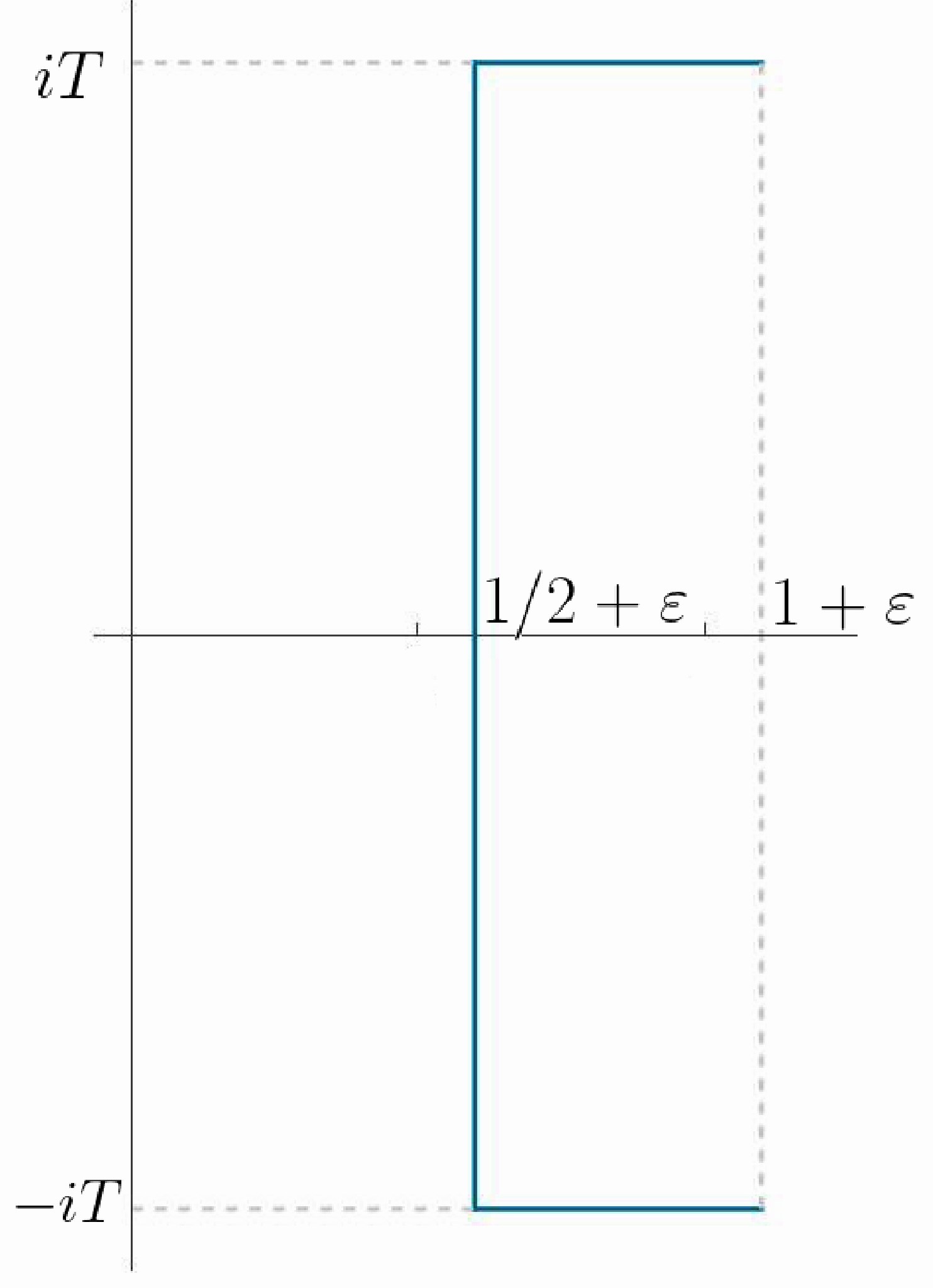
(a) Integration contour $\mathcal{C}$

From the Euler product expansion for $L(s,\chi)$ it is immediate that for $s=\sigma+it,\sigma>1$, one has $\absolutevalue{L(s,\chi)}\geq\zeta(2\sigma)/\zeta(\sigma)$, and thus $\absolutevalue{1/L(2s,\chi^{2})}\ll_{\varepsilon}1$ everywhere on the above contour. Moreover, from the above discussion, we also have $H_{\chi}(s)\ll 1$. Hence

$$\frac{1}{2\pi i}\int_{\mathcal{C}}\mathcal{L}_{\chi}(s)\frac{Z^{s}}{s}ds\ll_{\varepsilon}\int_{\mathcal{C}}\absolutevalue{L(s,\chi))}\frac{Z^{s}}{s}ds.$$

Next, let $\chi^{\prime}$ be the the real primitive character of modulus $m_{0}<m$ that gives rise to $\chi$. For $\sigma>0$,

$$L(s,\chi)=L(s,\chi^{\prime})\prod_{p|m}(1+\chi^{\prime}(p)p^{-s})$$

and thus for $s\in\mathcal{C}$,

$$\absolutevalue{L(s,\chi)}\leq\absolutevalue{L(s,\chi^{\prime})}\prod_{p|m}(1+p^{-1/2-\varepsilon})\ll m^{\varepsilon}\absolutevalue{L(s,\chi^{\prime})}$$

From result of Davenport ([2]) that for $\chi^{\prime}$ primitive and $s=\sigma+it$, $\sigma\in[0,1]$, we have

$$\absolutevalue{L(s,\chi^{\prime})}\ll((\absolutevalue{t}+1)m_{0})^{1/2-\sigma/2}$$

Thus,

$$\int_{1/2+\varepsilon-iT}^{1/2+\varepsilon+iT}\absolutevalue{L(s,\chi^{\prime}))\frac{Z^{s}}{s}}ds\ll Z^{1/2+\varepsilon}m^{1/4-\varepsilon/2}\int_{-T}^{T}\frac{t^{1/4-\varepsilon/2}}{\absolutevalue{t}+1}dt\ll Z^{1/2+\varepsilon}\int_{1}^{T}t^{-3/4-\varepsilon}dt\ll m_{0}^{1/4-\varepsilon/2}Z^{1/2+\varepsilon}T^{1/4-\varepsilon}$$

Next, let $\sigma\geq 1$ and $s=\sigma+it,t>1$, and let

$$A(u):=\sum_{n\leq u}\chi^{\prime}(n).$$

If $\chi$ is principal (i.e., if $L(s,\chi^{\prime})=\zeta(s)$) one has $\absolutevalue{L(s,\chi^{\prime})}\ll\log\absolutevalue{t}$. Indeed, for an integer $N=\lfloor T\rfloor$, Abel summation gives

$$\zeta(s)=\sum_{n\leq N}n^{-s}-N^{s-1}+\int_{N}^{\infty}\frac{su}{u^{s+1}}du-\int_{N}^{\infty}\frac{s\{u\}}{u^{s+1}}du=\sum_{n\leq N}n^{-s}+\mathrm{O}(1)+\mathrm{O}\left(T/N\right)=\mathrm{O}(\log T).$$

On the other hand, if $\chi$ is non-principal, one has

$$\absolutevalue{A(u)}\ll\sqrt{m_{0}}\log m_{0}$$

by the Polya-Vinogradov inequality; hence, by partial summation,

$$\absolutevalue{\sum_{n\geq N}n^{-s}\chi^{\prime}(n)}=\absolutevalue{-A(N)N^{-s}+\int_{N}^{\infty}\frac{sA(u)}{u^{s+1}}du}\ll\frac{\sqrt{m_{0}}\log m_{0}}{N}+\absolutevalue{t}\sqrt{m_{0}}\log m_{0}\int_{N}^{\infty}\frac{du}{u^{s+1}}\ll\frac{\absolutevalue{t}\sqrt{m_{0}}\log m}{N},$$

so setting $N=\sqrt{m_{0}}\absolutevalue{t}$, we see that

$$\absolutevalue{L(s,\chi^{\prime})}\ll\absolutevalue{\sum_{n<N}\chi^{\prime}(n)n^{-s}}+\absolutevalue{t}\sqrt{m_{0}}\log m_{0}/N\ll\log\absolutevalue{m_{0}t}.$$

To summarize,

$$\int_{1/2+\varepsilon+iT}^{1+\varepsilon+iT}\absolutevalue{L(s,\chi^{\prime}))\frac{Z^{s}}{s}}ds \ll\int_{1/2+\varepsilon}^{1}\frac{Z^{\sigma}}{T}(Tm_{0})^{1/2-\sigma/2}d\sigma+\log(Tm_{0})\int_{1}^{1+\varepsilon}\frac{Z^{\sigma}}{T}d\sigma$$

$$\ll\frac{\sqrt{m_{0}}}{\sqrt{T}}\int_{1/2+\varepsilon}^{1}\left(\frac{Z}{\sqrt{Tm_{0}}}\right)^{\sigma}d\sigma+\frac{\varepsilon Z^{1+\varepsilon}\log m_{0}T}{T}$$

$$\ll\frac{Z}{T}+\frac{\varepsilon Z^{1+\varepsilon}\log Tm_{0}}{T}$$

and similarly for the other horizontal contour. Finally, taking $T=Z^{2/5}/m_{0}^{1/5}$ yields the desired error term. ∎

Lemma 6.8.

One has

$$\sum_{n\leq Z}\mu^{2}(n)\varphi(n)=\frac{Z^{2}}{2\zeta(2)}\prod_{p}\left(1-\frac{1}{p^{2}+p}\right)+\mathrm{O}(Z^{8/5+\varepsilon})$$

Proof.

Consider the associated Dirichlet series

$$\mathcal{L}_{\chi}(s):=\prod_{p}\left(1+\frac{p-1}{p^{2}}\right)=\frac{\zeta(s-1)}{\zeta(2s-2)}\prod_{p}\left(1-\frac{1}{p^{s}+p}\right).$$

Applying Perron’s formula again,

$$\sum_{N\leq Z}\mu^{2}(N)\chi(N)=\frac{1}{2\pi i}\int_{2+\varepsilon-iT}^{2+\varepsilon+iT}\mathcal{L}_{\chi}(s)\frac{Z^{s}}{s}ds+\mathrm{O}_{\varepsilon}\left(\frac{Z^{1+\varepsilon}}{T}\right)$$

Shifting the contour to the line $\real(s)=3/2+\varepsilon$ picks up the pole of $\zeta(s)$ at $s=2$ with residue agreeing with the main term, and no other poles. In the region $\real(s)\geq 3/2+\varepsilon$, the function $\prod_{p}\left(1-\frac{1}{p^{s}+p}\right)$ is bounded absolutely. Similarly, $\absolutevalue{1/\zeta(2s-2)}\ll_{\varepsilon}1$ in this region. Hence it suffices to bound the contour integrals $\int_{1/2+\varepsilon-iT}^{1/2+\varepsilon+iT}\absolutevalue{\zeta(s)Z^{s+1}/s}ds$ and $\int_{1/2+\varepsilon\pm iT}^{1+\varepsilon\pm iT}\absolutevalue{\zeta(s)Z^{s+1}/s}ds$. By the convexity bound we have $\zeta(1/2+\varepsilon+it)\ll(1+\absolutevalue{t})^{1/2-\sigma/2}$; hence, for the first integral

$$\int_{1/2+\varepsilon-iT}^{1/2+\varepsilon+iT}\absolutevalue{\zeta(s)Z^{s+1}/s}ds\ll Z^{3/2+\varepsilon}\int_{1}^{T}t^{1/4-\varepsilon/2-1}dt=Z^{3/2+\varepsilon}T^{1/4-\varepsilon/2}.$$

Similarly, on the vertical parts of the contour inside the critical strip, one has

$$\int_{1/2+\varepsilon+iT}^{1+iT}\absolutevalue{\zeta(s)Z^{s+1}/s}ds\ll\int_{1/2+\varepsilon}^{1}Z^{t+1}\frac{T^{1/2-t/2}}{T}dt\ll\frac{Z^{2}}{T}\int_{0}^{1/2}T^{-t/2}\ll Z^{2}/T,$$

and for $\sigma\geq 1$, $\zeta(s)=\mathrm{O}(\log T)$ gives

$$\int_{1+iT}^{1+\varepsilon+iT}\absolutevalue{\zeta(s)Z^{s+1}/s}ds\ll\varepsilon Z^{2+\varepsilon}/T^{1-\varepsilon}.$$

Taking $T=Z^{2/5}$ concludes the calculation.

∎

7 Acknowledgments

I am very grateful to Andrew Sutherland for introducing this question and to Peter Sarnak for suggesting it as a project to me, as well as for many fruitful discussions. I would like to thank Jonathan Bober, Andrew Booker, Andrew Granville, Yang-Hui He, Min Lee, Michael Lipnowski, Mayank Pandey, Michael Rubinstein, and Will Sawin, for enlightening conversations in connection to this problem.

The research was supported by NSF GRFP and the Hertz Fellowship.

References

- [1] Raymond Ayoub. An introduction to the analytic theory of numbers. Mathematical Surveys, No. 10. American Mathematical Society, Providence, R.I., 1963.
- [2] H. Davenport. On Dirichlet’s L-Functions. J. London Math. Soc., 6(3):198–202, 1931.
- [3] Yang-Hui He, Kyu-Hwan Lee, Thomas Oliver, and Alexey Pozdnyakov. Murmurations of elliptic curves. 2022.
- [4] Yang-Hui He, Kyu-Hwan Lee, Thomas Oliver, Alexey Pozdnyakov, and Andrew V. Sutherland. In preparation.
- [5] C. Hooley. A note on square-free numbers in arithmetic progressions. Bull. London Math. Soc., 7:133–138, 1975.
- [6] Nicholas M. Katz and Peter Sarnak. Zeroes of zeta functions and symmetry. Bull. Amer. Math. Soc. (N.S.), 36(1):1–26, 1999.
- [7] Greg Martin. Dimensions of the spaces of cusp forms and newforms on and . J. Number Theory, 112(2):298–331, 2005.
- [8] Kimball Martin. Root number bias for newforms. Proc. Amer. Math. Soc., 151(9):3721–3736, 2023.
- [9] Kimball Martin and Thomas Pharis. Rank bias for elliptic curves mod . Involve, 15(4):709–726, 2022.
- [10] Kimball Martin and Thomas Pharis. Errata for rank bias for elliptic curves mod . https://math.ou.edu/~kmartin/papers/aprank-err.pdf, 2023.
- [11] Peter Sarnak. Letter to Drew Sutherland and Nina Zubrilina on murmurations and root numbers. https://publications.ias.edu/sarnak/paper/2726, 2023.
- [12] Nils-Peter Skoruppa and Don Zagier. Jacobi forms and a certain space of modular forms. Invent. Math., 94(1):113–146, 1988.
- [13] Andrew V. Sutherland. Letter to Michael Rubinstein and Peter Sarnak. https://math.mit.edu/~drew/RubinsteinSarnakLetter.pdf, 2022.
- [14] Andrew V. Sutherland. Murmurations of weight newforms for , comparison to theorem. https://math.mit.edu/~drew/zub8.html, 2023.
- [15] E. C. Titchmarsh. The theory of the Riemann zeta-function. The Clarendon Press, Oxford University Press, New York, second edition, 1986. Edited and with a preface by D. R. Heath-Brown.
- [16] Masatoshi Yamauchi. On the traces of Hecke operators for a normalizer of . J. Math. Kyoto Univ., 13:403–411, 1973.