Hamiltonian Dynamics of Bayesian Inference
Formalised by Arc Hamiltonian Systems

Supplemental Material for ‘Hamiltonian Dynamics of Bayesian Inference Formalised by Arc Hamiltonian Systems’

Abstract

This paper advances theoretical understanding of infinite-dimensional geometrical properties associated with Bayesian inference. First, we introduce a novel class of infinite-dimensional Hamiltonian systems for saddle Hamiltonian functions whose domains are metric spaces. A flow of this system is generated by a Hamiltonian arc field, an analogue of Hamiltonian vector fields formulated based on (i) the first variation of Hamiltonian functions and (ii) the notion of arc fields that extends vector fields to metric spaces. We establish that this system obeys the conservation of energy. We derive a condition for the existence of the flow, which reduces to local Lipschitz continuity of the first variation under sufficient regularity. Second, we present a system of a Hamiltonian function, called the minimum free energy, whose domain is a metric space of negative log-likelihoods and probability measures. The difference of the posterior and the prior of Bayesian inference is characterised as the first variation of the minimum free energy. Our result shows that a transition from the prior to the posterior defines an arc field on a space of probability measures, which forms a Hamiltonian arc field together with another corresponding arc field on a space of negative log-likelihoods. This reveals the underlying invariance of the free energy behind the arc field.

1 Introduction

In Bayesian inference, statisticians elicit a prior distribution $P$ over a parameter space $\Theta$ of a model that reflects their belief in an appropriate model to describe a phenomenon of interest. Observing data realised from the phenomenon, they update the prior distribution $P$ to the posterior distribution $P_{*}$ by Bayes’ rule. Denote the negative log-likelihood by $f:\Theta\to\mathbb{R}$, making the associated model and data implicit. Most generally, the posterior $P_{*}$ is a measure absolutely continuous to $P$ that has the Radon–Nikodym derivative

$$\frac{dP_{*}}{dP}(\theta)=\frac{\exp(-f(\theta))}{\int_{\Theta}\exp(-f(\theta))dP(\theta)}.$$ (1)

If the prior $P$ admits a probability density $p$, the posterior $P_{*}$ can be expressed as a probability density $p_{*}(\theta)\propto\exp(-f(\theta))p(\theta)$ as usual. The measure $P_{*}$ of the form (1) is also known as a Gibbs measure for a potential $f$ with a reference measure $P$ (Georgii, 2011).

The posterior, or the Gibbs measure, has a variational characterisation whose origin may be traced back to Gibbs (1902). It is a unique solution of the following variational problem:

$$P_{*}=\operatorname*{arg\,min}_{Q\in\mathcal{P}}\mathcal{F}(Q)\quad\text{for}\quad\mathcal{F}(Q)=\int_{\Theta}f(\theta)dQ(\theta)+\operatorname{KL}(Q,P)$$ (2)

where $\mathcal{P}$ denotes a set of all probability measures on $\Theta$ and $\operatorname{KL}(Q,P)$ denotes the relative entropy of $Q$ from $P$. The functional $\mathcal{F}$ is called the free energy in light of the thermodynamical significance. This characterisation has been long known as the Gibbs variational principle (Ellis, 2006) mainly in the context of statistical mechanics (Ruelle, 1967, 1969) and large deviation theory (Dembo and Zeitouni, 2009; Dupuis and Ellis, 2011). Later, it was repeatedly rediscovered and has played a pivotal role in several recent advances of Bayesian inference, such as variational Bayes methods (Attias, 1999; Blei, Kucukelbir and McAuliffe, 2017), PAC-Bayes analysis (Catoni, 2007; Guedj, 2019), and generalised Bayesian inference (Bissiri, Holmes and Walker, 2016). This paper establishes (i) a further variational characterisation of the posterior $P_{*}$ and (ii) its Hamiltonian dynamical interpretation.

Hamiltonian systems are a fundamental description of dynamical phenomena that obey the law of conservation of energy (Goldstein, Poole and Safko, 2002). A flow of a Hamiltonian system is generated by the Hamiltonian vector field determined by the gradient of a Hamiltonian function. Under sufficient regularity, the value of the Hamiltonian function remains invariant along the flow (Abraham and Marsden, 1987). While Hamiltonian systems are well-established for finite-dimensional topological spaces (Arnold, 1978), this work deals with saddle (i.e. concave-convex) Hamiltonian functions whose domains are infinite-dimensional metric spaces. A chief challenge in formulating Hamiltonian systems in such a setting is to have (a) an appropriate notion that acts as a gradient in an infinite-dimensional domain and (b) the well-defined evolution of a system in a metric topology. To date, Hamiltonian systems have been extended to Banach spaces—or symplectic manifolds built on smooth Banach manifolds (Lang, 1985) more generally—by works of Chernoff and Marsden (1974); Marsden and Hughes (1983). A formulation based on a norm topology is however not suitable for our main application involving dynamics of measures, as illustrated in Section 2. This motivates the development of a novel class of Hamiltonian systems, termed arc Hamiltonian systems, using (a) the first variation of Hamiltonian functions and (b) the notion of arc fields (Calcaterra and Bleecker, 2000) that extends vector fields to metric spaces. A flow of an arc Hamiltonian system is generated by the Hamiltonian arc field determined by the first variation of a Hamiltonian function. We provide a condition for the existence of the flow over $[0,\infty)$, and prove that this system obeys the conservation of energy.

We use arc Hamiltonian systems to study an infinite-dimensional geometrical property associated with Bayesian inference. Denote $f^{c}(\theta):=f(\theta)-\int_{\Theta}f(\theta)dP(\theta)$ for simpler presentation. We shall see that the difference of the posterior $P_{*}$ and the prior $P$ is characterised as the first variation of the minimum free energy $H(f,P)$ with respect to $f$:

$$P_{*}-P=\frac{\partial}{\partial f}H(f,P)\quad\text{for}\quad H(f,P)=-\log\left(\int_{\Theta}\exp\left(-f^{c}(\theta)\right)dP(\theta)\right)$$ (3)

where the first variation here, formally defined in Section 3, is similar to one often considered in the context of gradient flows (Santambrogio, 2015). We shall show that the first variation $(\partial/\partial f)H(f,P)$, coupled with the negative of the other first variation $-(\partial/\partial P)H(f,P)$ with respect to $P$, defines an arc Hamiltonian field on a metric space $(M,d)$ of negative log-likelihoods $f$ and probability measures $P$. It generates a flow $t\mapsto(f_{t},P_{t})$ of the system that follows the first-order approximation similar to Hamilton’s equations in vector spaces:

$$(f_{t+s},P_{t+s})\approx(f_{t},P_{t})+s\left(-\frac{\partial}{\partial P}H(f_{t},P_{t}),\frac{\partial}{\partial f}H(f_{t},P_{t})\right).$$ (4)

Our formulation capitalises on a property that the right-hand side stays within the domain $M$ of the energy $H(f,P)$ for all $s\in[0,1]$, due to the form of the first variations. In such cases, the first-order approximation (4) can determines a flow in a metric topology.

The first-order approximation (4) of $P_{t+s}$ driven by the first variation $(\partial/\partial f)H(f_{t},P_{t})=P_{*}-P_{t}$ is a transition from $P_{t}$ to $P_{*}$ over $s\in[0,1]$ in the mixture geodesic $(1-s)P_{t}+sP_{*}$, where the posterior $P_{*}$ is defined for $(f_{t},P_{t})$. By the belief updating mechanism of Bayesian inference, we can assign this transition $(1-s)P+sP_{*}$ over $s\in[0,1]$ to every probability measure $P$. Our result confers the geometrical significance of such an assignment at every $P$ as a Hamiltonian arc field, by introducing another transition $f-s(\partial/\partial P)H(f,P)$ driven by the other first variation $(\partial/\partial P)H(f,P)$. In particular, this reveals an underlying invariance of the minimum free energy $H(f,P)$ behind the arc field induced by the belief updating mechanism. See Figure 1 for illustration of this dynamics.

Certainly, there can exist various geodesics to define a transition from $P$ to $P_{*}$. Finally, it is intriguing to highlight a contrast with a Wasserstein gradient flow of the free energy $\mathcal{F}$ (Jordan, Kinderlehrer and Otto, 1997). The Wasserstein dynamics describes the evolution of a probability measure $Q_{t}$ over time $t$ that minimises the free energy $\mathcal{F}(Q_{t})\to\mathcal{F}(P_{*})$ for a fixed potential $f$ with reference measure $P$. We have the same Wasserstein dynamics for a class of free energies $\mathcal{F}$ of potentials $f-C$ up to a constant $C$. We suppose that the free energy $\mathcal{F}$ is defined with a ‘mean-zero’ potential $f^{c}(\theta)=f(\theta)-C$ with $C=\int_{\Theta}f(\theta)dP(\theta)$. The minimum free energy $H(f,P)$ equals to the free energy $\mathcal{F}(P_{*})$ at the minimiser $P_{*}$:

$$H(f,P)=-\log\left(\int_{\Theta}\exp(-f^{c}(\theta))dP(\theta)\right)=\int_{\Theta}f^{c}(\theta)dP_{*}(\theta)+\operatorname{KL}(P_{*},P)=\mathcal{F}(P_{*})$$

where this equality is known as the Gibbs or Donsker-Varadhan variational formula (Dupuis and Ellis, 2011). In contrast to the Wasserstein dynamics that minimises the free energy $\mathcal{F}(Q_{t})\to\mathcal{F}(P_{*})$, our result reveals the existence of the dynamics of the potential $f_{t}$ and reference measure $P_{t}$ that keeps the minimised free energy $H(f_{t},P_{t})=\mathcal{F}(P_{*})$ constant.

The rest of the paper is structured as follows. Section 2 introduces basic notations and useful preliminaries for the development of arc Hamiltonian systems. In Section 3, we establish the framework of arc Hamiltonian systems, providing the theory on the existence and the energy-conserving invariance of their flow. The general framework of arc Hamiltonian systems may be of independent interest in many fields, such as convex analysis, information theory, and statistical physics. In Section 4, we present the system of the minimum free energy formalised by arc Hamiltonian systems. We draw our conclusion in Section 5.

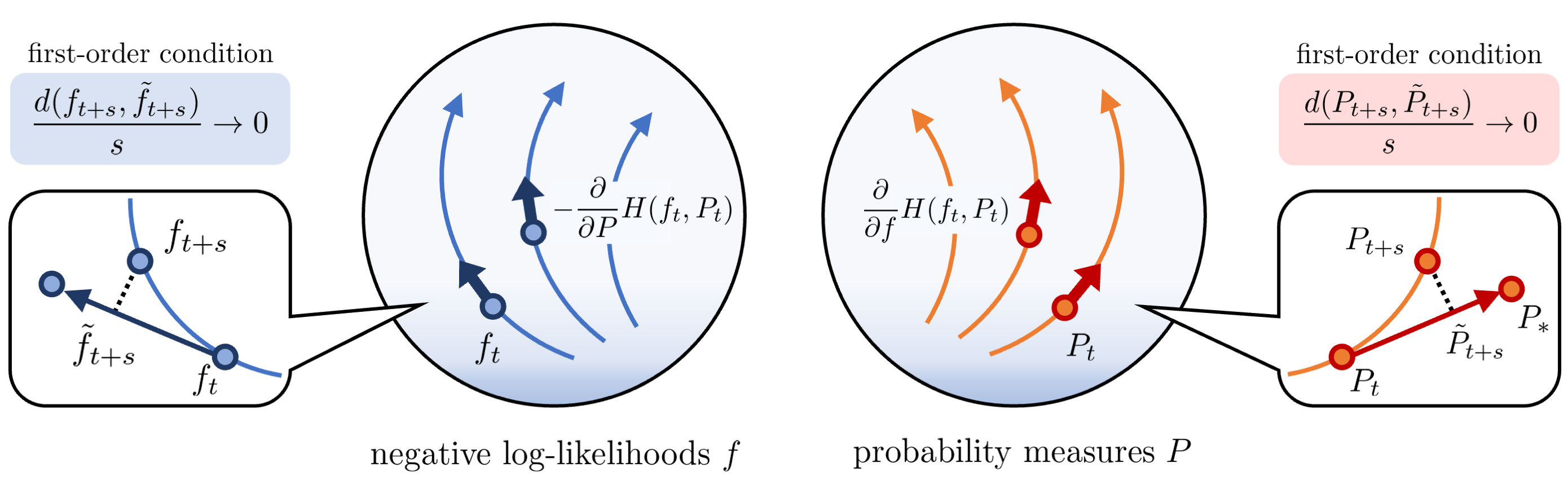
Figure 1: Illustration of the arc Hamiltonian system of the minimum free energy. Any generated flow $t\mapsto(f_{t},P_{t})$ of the system over $t\in[0,\infty)$ conserves the minimum free energy $H(f_{t},P_{t})$.

2 Background

We provide useful preliminaries to develop arc Hamiltonian systems. Section 2.1 introduces a set of basic notations and terminologies. Section 2.2 briefly recaps a standard Hamiltonian system in the Euclidean space $\mathbb{R}^{d}$, illustrating a few limitations of an infinite-dimensional extension based on a norm topology for our application. Finally, Section 2.3 recaps the notion of arc fields established by Calcaterra and Bleecker (2000), which we capitalise on to formulate the evolution of an arc Hamiltonian system in a metric topology.

2.1 Notations and Terminologies

We introduce basic notations and terminologies.

Functional-Analytic

By a “curve”, we mean a map from a time interval to a metric space, where it can be equivalently thought of as a time-dependent variable in a metric space. We use subscripts to indicate the time argument of a curve; for example $t\mapsto x_{t}$ denotes a curve. A curve is said continuous if it is a continuous map. We denote by $\lim_{s\to 0^{+}}$ the limit with respect to a scalar $s\in\mathbb{R}$ approaching to $0$ from the right. For any metric space $(M,d)$, we denote by $B_{r}(x)$ an open ball in $(M,d)$ around a point $x\in M$ with a radius $r$. For any map $\Phi:M\times[0,1]\to M$ defined for a set $M$ and the time interval $[0,1]$, we use subscripts to indicate the time argument of $\Phi$, that is, $\Phi_{s}(x)$ denotes the value at $(x,s)\in M\times[0,1]$.

Measure-Theoretic

Let $\Theta$ be a separable completely metrizable space (i.e. a Polish space). By a “measure”, we mean a non-negative Borel measure on $\Theta$. By a “signed measure”, we mean a signed Borel measure on $\Theta$. Any signed measure $P$ admits the Jordan decomposition $P=P^{+}-P^{-}$ by two uniquely associated (non-negative) measures $P^{+}$ and $P^{-}$. For each signed measure $P$, we define a measure $|P|$—often referred to as the variation of $P$— by $|P|:=P^{+}+P^{-}$. This means that $\int_{O}d|P|(\theta)=\int_{O}dP^{+}(\theta)+\int_{O}dP^{-}(\theta)$ for any Borel set $O\subseteq\Theta$. A signed measure $P$ is said finite if and only if the measure $|P|$ is finite. If a measure $P$ admits the Radon-Nikodym derivative $h$ with respect to a measure $Q$, we indicate the relationship by $dP(\theta)=h(\theta)dQ(\theta)$ for better presentation. Denote by $\mathcal{M}$, $\mathcal{M}^{+}$, and $\mathcal{P}$ a set of all finite signed measures, all finite measures, and all probability measures.

2.2 Hamiltonian Systems

Hamiltonian systems have an extensive history of the development; we refer readers to Goldstein, Poole and Safko (2002) for a detailed introduction of classical mechanics and to Arnold (1978) for the rigorous mathematical foundation. Hamiltonian systems enable us to describe the evolution of the objects through the first-order evolution equation, by introducing a variable called the momentum. For illustration, consider an object moving in $\mathbb{R}^{d}$ whose location at time $t$ is denoted $x_{t}\in\mathbb{R}^{d}$. The momentum, denoted $z_{t}\in\mathbb{R}^{d}$, can be associated with a physical quantity calculated by the product of the mass and velocity at time $t$. A Hamiltonian function $H:\mathbb{R}^{d}\times\mathbb{R}^{d}\to\mathbb{R}$ corresponds to the total energy that the system has at each state $(x,z)$. How the pair of the location and momentum $(x_{t},z_{t})$ evolves over time $t$ is determined through Hamilton’s equation:

$$\frac{d}{dt}(x_{t},z_{t})=(-\nabla_{2}H(x_{t},z_{t}),\nabla_{1}H(x_{t},z_{t}))$$ (5)

where $\nabla_{1}$ and $\nabla_{2}$ denote the gradient operator with respect to the first and second argument. Hamilton’s equation (5) is a differential equation $(d/dt)(x_{t},z_{t})=F(x_{t},z_{t})$ driven by the Hamiltonian vector field $F(x,z)=(-\nabla_{2}H(x,z),\nabla_{1}H(x,z))$, which can be solved as an initial value problem. Under sufficient regularity, it generates a unique solution flow $t\mapsto(x_{t},z_{t})$ from any initial state $(x_{0},z_{0})$ in the domain $\mathbb{R}^{d}\times\mathbb{R}^{d}$. In particular, any flow $t\mapsto(x_{t},z_{t})$ generated by the Hamiltonian vector field conserves the energy, meaning that the value of the Hamiltonian function $H(x_{t},z_{t})$ remains constant along the flow. Figure 2 illustrates a Hamiltonian system of a simple pendulum; it can be observed that the values of the Hamiltonian function remain constant along every generated flow.

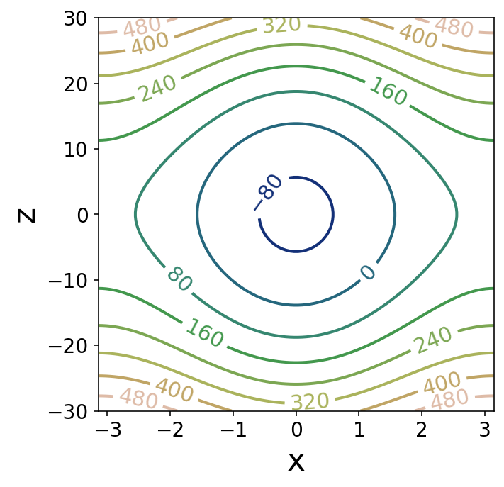
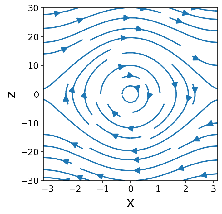
Figure 2: The Hamiltonian system of a simple pendulum whose rod length and mass are both $1$. (Left) The Hamiltonian function $H(x,z)=z^{2}/2-g^{2}\cos(x)$ for each angle $x\in[-\pi,\pi]$ and momentum $z\in\mathbb{R}$ of the pendulum, where $g$ is the standard acceleration of gravity. (Right) A flow by Hamilton’s equation $(d/dt)(x_{t},z_{t})=(z_{t},-g^{2}\sin(x_{t}))$ from each initial state.

Chernoff and Marsden (1974)—and later Marsden and Hughes (1983) for application to mechanics of elastic materials—established an infinite-dimensional extension of Hamiltonian systems to Banach spaces and, more generally, to symplectic manifolds built on smooth Banach manifolds. Here, we do not consider the case of Banach manifolds. As Kriegl and Michor (1997) and Schmeding (2022) pointed out, there are known limitations of Banach manifolds. For example, Eells and Elworthy (1970) proved that an infinite-dimensional smooth Banach manifold is smoothly embedded as an open set in a Banach space used to define the atlas. Analysis on smooth Banach manifolds then reduces to that on Banach spaces.

Consider a setting where an object of interest $(x_{t},z_{t})$ belongs to a Banach space $E_{1}\times E_{2}$. In the extended Hamiltonian system, the evolution of the system is governed by an evolution equation $(d/dt)(x_{t},z_{t})=F(x_{t},z_{t})$ driven by a map $F:E_{1}\times E_{2}\to E_{1}\times E_{2}$ which depends on the gradient of the Hamiltonian function $H(x,z)$ analogous to (5) but taken in a sense of the Fréchet derivative under appropriate conditions of $E_{1}$ and $E_{2}$. By the Cauchy-Lipschitz theorem (e.g. Brezis, 2011), the evolution equation admits a unique solution from any initial state if the map $F$ is Lipschitz continuous in $E_{1}\times E_{2}$. However, this formulation based on a norm topology is not suitable for dynamics involving the set of measures $\mathcal{M}^{+}$. In a Banach space of signed measures $\mathcal{M}$ under e.g. the total variation norm $\|\cdot\|_{\mathcal{M}}$ (Cohn, 2013), it is easy to prove that the subset $\mathcal{M}^{+}$ has no interior point. That is, if we use the norm topology on $\mathcal{M}$, no open set can be defined inside $\mathcal{M}^{+}$ to use important topological notions—such as the Fréchet derivative or local Lipschitz continuity—of functions defined only on $\mathcal{M}^{+}$. One trivial approach to define open sets inside $\mathcal{M}^{+}$ is to use a metric topology on $\mathcal{M}^{+}$ instead of the norm topology introduced to the vector space $\mathcal{M}$. For example, the set $\mathcal{M}^{+}$ will be a metric space $(\mathcal{M}^{+},d)$ under the total variation metric $d$ on $\mathcal{M}^{+}$ defined by restricting the norm distance $\|P-Q\|_{\mathcal{M}}$ to $\mathcal{M}^{+}\times\mathcal{M}^{+}$. This motivates us to introduce a metric on the domain of interest and define the evolution within the metric space. To achieve this, we capitalise on the notion of arc fields (Calcaterra and Bleecker, 2000) recapped next.

2.3 Arc Fields

The notion of arc fields (Calcaterra and Bleecker, 2000), that extends vector fields to metric spaces, is used to formulate an analogue of Hamiltonian vector fields and Hamilton’s equation in metric spaces. The underlying idea behind arc fields has a close connection to mutational equations (Aubin, 1999; Lorenz, 2010) whose common application includes the evolution of set-valued objects and objects that belongs to complicated regions of vector spaces (Aubin, 1993). To illustrate the idea, consider a vector field $F:E\to E$ in a Banach space $(E,\|\cdot\|_{E})$ and a solution curve $t\mapsto x_{t}$ of the corresponding evolution equation $(d/dt)x_{t}=F(x_{t})$. At each $x\in E$, define a curve $\Phi_{s}(x)=x+sF(x)$ over time $s\in[0,1]$. Informally, the evolution equation can be thought of as the first-order approximation of the solution curve $x_{t+s}\approx\Phi_{s}(x_{t})$ at each $t$ over small $s$, specified by the curve $s\mapsto\Phi_{s}(x_{t})$:

$$\lim_{s\to 0}\left\|\frac{x_{t+s}-x_{t}}{s}-F(x_{t})\right\|_{E}=\lim_{s\to 0}\frac{\|x_{t+s}-\Phi_{s}(x_{t})\|_{E}}{|s|}=0.$$

A key observation is that the vector-space structure of the set $E$—where the curve $t\mapsto x_{t}$ belongs—is not essential in this formulation. In the above condition, consider that the vector space $E$ is replaced with any set, such as $\mathcal{M}^{+}$, and the norm $\|x_{t+s}-\Phi_{s}(x_{t})\|_{E}$ is replaced with a metric $d(x_{t+s},\Phi_{s}(x_{t}))$ on the replaced set $E$. The above condition can be still well-defined if we have a premise that the curve $s\mapsto\Phi_{s}(x_{t})$ stays within the set $E$ over all $s$ in some interval. This observation leads to the extension of vector fields to metric spaces.

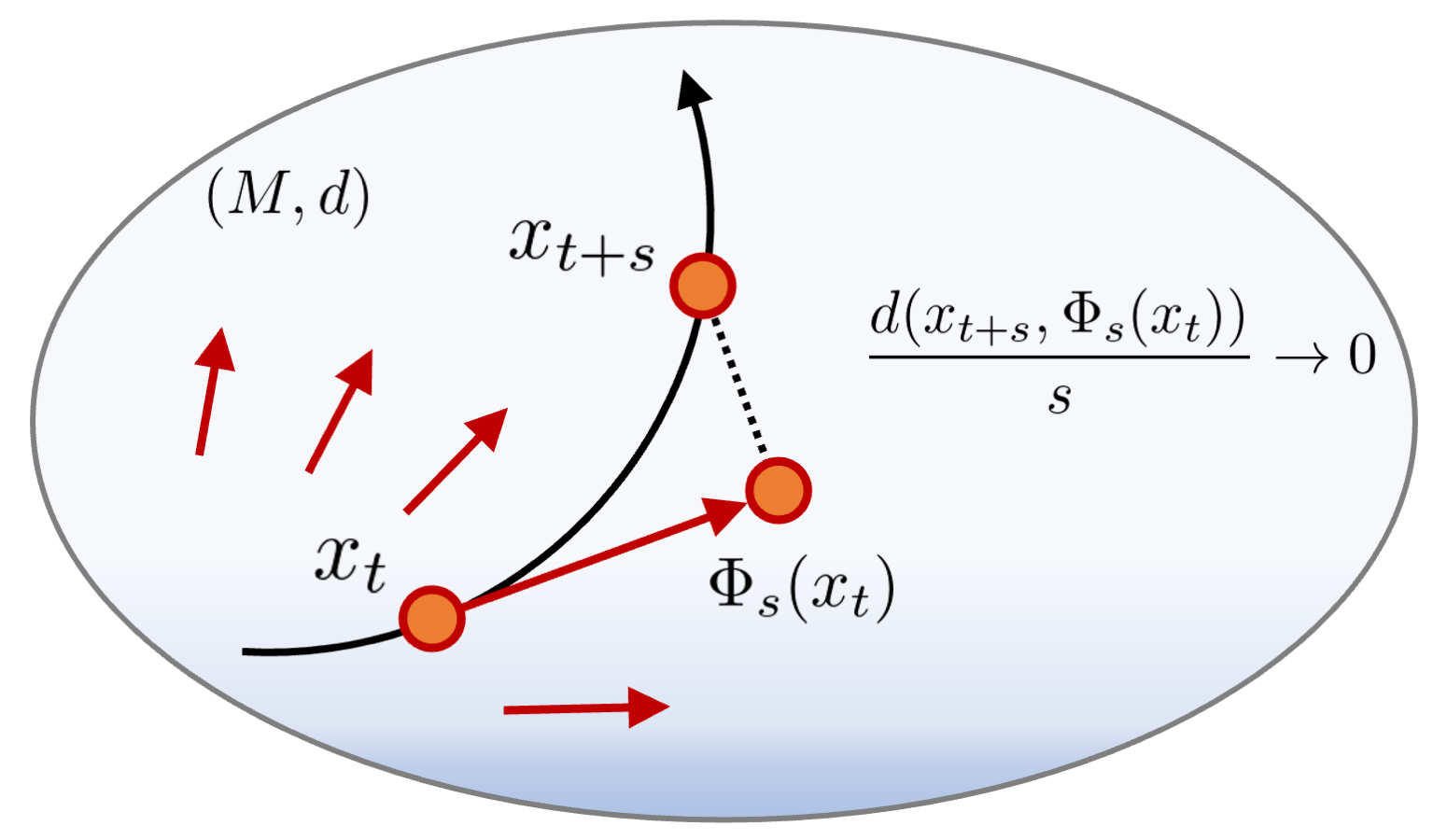
Figure 3: Illustration of the generation of a flow $t\mapsto x_{t}$ in a metric space $(M,d)$ by an arc field $\Phi:M\times[0,1]\to M$. A local approximation of the flow at time $t$ is specified by the curve $s\mapsto\Phi_{s}(x_{t})$ assigned to the point $x_{t}$ by the arc field, under the condition that the approximation error $d(x_{t+s},\Phi_{s}(x_{t}))$ converges faster than the linear order $s$ at each $x_{t}$.

Given a metric space $(M,d)$, consider a map $\Phi:M\times[0,1]\to M$ that satisfies $\Phi_{0}(x)=x$ for all $x\in M$, where we recall that $\Phi_{s}(x)$ denotes the value of $\Phi$ at $(x,s)\in M\times[0,1]$. To each point $x\in M$, this map $\Phi$ is considered to assign a curve $s\mapsto\Phi_{s}(x)$ over $s\in[0,1]$ in $(M,d)$ that starts from $x$. Calcaterra and Bleecker (2000) was concerned with the existence of a curve $t\mapsto x_{t}$ in $(M,d)$ that satisfies the following first-order approximation at each $t$:

$$\lim_{s\to 0^{+}}\frac{d(x_{t+s},\Phi_{s}(x_{t}))}{s}=0.$$ (6)

To study the existence, Calcaterra and Bleecker (2000) focused on a class of sufficiently regular maps $\Phi:M\times[0,1]\to M$, called arc fields, that satisfies a continuity condition in (7) below. A curve $t\mapsto x_{t}$ in $(M,d)$ from some initial point $x_{0}$ that satisfies the condition (6) of an arc field $\Phi$ over some interval $[0,T)$ is then called a solution of the arc field $\Phi$.

Definition 1 (Arc Field).

An arc field on a metric space $(M,d)$ is a map $\Phi:M\times[0,1]\to M$ that satisfies that $\Phi_{0}(x)=x$ for all $x\in M$ and that

$$\rho(x):=\sup_{t,s\in[0,1]\text{~{}s.t.~{}}t\neq s}\frac{d(\Phi_{t}(x),\Phi_{s}(x))}{|t-s|}<\infty\quad\text{and}\quad\bar{\rho}(x,r):=\sup_{v\in B_{r}(x)}\rho(v)<\infty$$ (7)

at each $x\in M$ for $r>0$ sufficiently small.

See Figure 3 for illustration of a solution of an arc field $\Phi$. See Appendix A for a summary of the theoretical results of Calcaterra and Bleecker (2000) relevant to the development of arc Hamiltonian systems. A flow of an arc Hamiltonian system is formulated as a unique continuous solution of the Hamiltonian arc field $\Phi$ associated with the system.

3 Arc Hamiltonian Systems

Extending Hamiltonian systems to infinite-dimensional metric spaces may open up a new horizon for formulating the dynamics of intriguing phenomena. A focus in this work is on saddle Hamiltonian functions whose domains are equipped with metrics. This section will establish the general framework of arc Hamiltonian systems. The first variation (c.f. Section 3.1) of a Hamiltonian function determines an arc field, called Hamiltonian arc field (c.f. Section 3.2), that generates a flow of the system in the metric space. It will be shown that the generated flow obeys the conservation of energy.

In Section 3.1, we present the definition of the first variation based on a convex-analytic formulation. In Section 3.2, we provide the rigorous construction of arc Hamiltonian systems. Section 3.3 shows the existence of a flow generated by a Hamiltonian arc field, followed by Section 3.4 establishing the conservation of energy by the generated flow. Under sufficient regularity, a condition of the existence of the energy-conserving flow reduces to local Lipschitz continuity of the first variation of a Hamiltonian function. Before moving on to the first subsection, we introduce convex-analytic preliminaries below.

Convex-Analytic Preliminaries

Define the extended real number $\overline{\mathbb{R}}:=\mathbb{R}\cup\{-\infty,\infty\}$. It is standard convention in convex analysis to consider extended-valued functions from a vector space $E$ to $\overline{\mathbb{R}}$. We denote by $\operatorname{Dom}(f)$ a subset of $E$ where an extended-valued function $f:E\to\overline{\mathbb{R}}$ takes a finite value in $\mathbb{R}$. An extended-valued function $f:E\to\overline{\mathbb{R}}$ is said convex if (i) $\operatorname{Dom}(f)$ is a non-empty convex set and (ii) $f((1-\lambda)x+\lambda v)\leq(1-\lambda)f(x)+\lambda f(v)$ holds for any $\lambda\in[0,1]$ and $x,v\in\operatorname{Dom}(f)$. An extended-valued function $f:E\to\overline{\mathbb{R}}$ is said concave if (i) $-f$ is convex. Any function $f:D\to\mathbb{R}$ defined on a subset $D$ of $E$ can be identified as an extended-valued function $f:E\to\overline{\mathbb{R}}$ by setting $f(x):=\infty$ for all $x\in E\setminus D$.

3.1 First Variations

The gradient of functions in a general topological space is characterised as an element of the topological dual. For example, the topological dual of $\mathbb{R}^{d}$ is identical to $\mathbb{R}^{d}$ itself and hence the gradient of functions in $\mathbb{R}^{d}$ belongs to $\mathbb{R}^{d}$. First, we recap definition of dual pair (Aliprantis and Border, 2006, Section 5.14) that plays a fundamental role in defining a gradient in infinite-dimensional convex analysis.

Definition 2 (Dual Pair).

A dual pair, denoted $\langle E_{1},E_{2}\rangle$, is a pair of vector spaces $E_{1}$ and $E_{2}$ together with a bilinear functional $\langle\cdot,\cdot\rangle:E_{1}\times E_{2}\to\mathbb{R}$ that satisfies

• if $\langle x,z\rangle=0$ for each $z\in E_{2}$, then $x=0$;

• if $\langle x,z\rangle=0$ for each $x\in E_{1}$, then $z=0$.

The bilinear functional $\langle\cdot,\cdot\rangle$ is called the duality of the dual pair $\langle E_{1},E_{2}\rangle$.

A dual pair $\langle E_{1},E_{2}\rangle$ equips each $E_{1}$ and $E_{2}$ with topologies—called the weak and weak^∗ topologies, respectively—that turn $E_{1}$ and $E_{2}$ into the topological dual of each other. A large class of vector spaces can be coupled as the mutual topological dual through an appropriate dual pair; see (Aliprantis and Border, 2006, Section 5.14) for examples of common dual pairs. A dual pair we consider in Section 4 is one for functions $f$ and measures $P$ in $\Theta$ whose duality is given by $\langle f,P\rangle=\int_{\Theta}f(\theta)dP(\theta)$ (e.g. Müller, 1997).

In the rest of Section 3, let $\langle E_{1},E_{2}\rangle$ be an arbitrary dual pair. It suffices to consider convex or concave functions $f:E_{1}\to\overline{\mathbb{R}}$ to define a gradient we use for saddle Hamiltonian function. The directional derivative $Df_{x}(v)$ of $f$ at $x$ in direction $v\in E_{1}$ is defined by

$$Df_{x}(v):=\lim_{\lambda\to 0^{+}}\frac{f(x+\lambda v)-f(x)}{\lambda}.$$ (8)

One of the most common notions of gradients in infinite-dimensional convex analysis is the Gâteaux gradient. If there exists a unique element $\partial f(x)\in E_{2}$ s.t. the limit of (8) satisfies

$$Df_{x}(v)=\langle v,\partial f(x)\rangle\quad\text{for all}\quad v\in E_{1},$$ (9)

the unique element $\partial f(x)\in E_{2}$ is called the Gâteaux gradient of $f$ at $x$. The linear functional $Df_{x}:E_{1}\to\mathbb{R}$ is called the Gâteaux derivative of $f$ at $x$. A gradient we use is a weaker version of the Gâteaux gradient that requires the equality (9) to hold only for directions $v$ s.t. $x+\lambda v$ stays within $\operatorname{Dom}(f)$ over all $\lambda\in[0,1]$. This ensures that the value of $f(x+\lambda v)$ in the directional derivative (8) is finite for all small $\lambda\geq 0$ to take the limit in $\lambda\to 0^{+}$. Such a version is often used and called first variation in the context of Wasserstein gradient flows (e.g. Santambrogio, 2015, Chapter 7.2) for functions whose domain is a set of probability measures $\mathcal{P}$ in the vector space of the signed measures $\mathcal{M}$. What first variation refers to may differ in each field. Now, we introduce our definition of first variation.

Definition 3 (First Variation).

Given a convex or concave function $f:E_{1}\to\overline{\mathbb{R}}$, let $C(x)$ denote a set $\{v\in E_{1}\mid x+v\in\operatorname{Dom}(f)\}$ at each $x\in\operatorname{Dom}(f)$. If there exists a unique element $\partial f(x)\in E_{2}$ s.t. the directional derivative of $f$ at $x\in\operatorname{Dom}(f)$ in (8) satisfies that

$$Df_{x}(v)=\langle v,\partial f(x)\rangle\quad\text{for all}\quad v\in C(x),$$ (10)

we call the unique element $\partial f(x)\in E_{2}$ the first variation of $f$ at $x$. We refer the function $Df_{x}:C(x)\to\mathbb{R}$ to as the variational derivative of $f$ at $x$.

Note that, if $v\in C(x)$, we have $x+\lambda v\in\operatorname{Dom}(f)$ for all $\lambda\in[0,1]$ because $x+\lambda v$ is expressed as a convex combination $(1-\lambda)x+\lambda(x+v)$ in the convex set $\operatorname{Dom}(f)$. Note also that the set $C(x)$ is never empty; given any $u\in\operatorname{Dom}(f)$, a point $u-x$ is a trivial element of $C(x)$. If $C(x)=E_{1}$, the first variation coincides with the Gâteaux gradient by definition.

Remark 1.

The first variation are immediately defined for convex or concave functions in the other space $E_{2}$ by interchanging the symbols $E_{1}$ and $E_{2}$ throughout Definition 3 and replacing $Df_{x}(v)=\langle v,\partial f(x)\rangle$ with $Df_{x}(v)=\langle\partial f(x),v\rangle$ in (10).

3.2 Definition of Arc Hamiltonian Systems

Hamiltonian systems describe the dynamics of a paired variable $(x_{t},z_{t})$ in some space. We consider a setting where the variable $(x_{t},z_{t})$ belongs to a subset $M$ in the product space $E_{1}\times E_{2}$. A Hamiltonian function $H:M\to\mathbb{R}$ on $M$ is regarded as an extended-valued function $H:E_{1}\times E_{2}\to\overline{\mathbb{R}}$ in convex-analytic manner.

The framework of arc Hamiltonian systems is developed for saddle Hamiltonian functions. An extended-valued function $H:E_{1}\times E_{2}\to\overline{\mathbb{R}}$ is said saddle if, at each $(x,z)\in\operatorname{Dom}(H)$,

• for fixed $z$, the function $H(\cdot,z):E_{1}\to\overline{\mathbb{R}}$ is concave;

• for fixed $x$, the function $H(x,\cdot):E_{2}\to\overline{\mathbb{R}}$ is convex.

Denote by $\partial_{1}H(x,z)\in E_{2}$ the first variation of the concave function $H(\cdot,z):E_{1}\to\overline{\mathbb{R}}$ at $x$. Denote by $\partial_{2}H(x,z)\in E_{1}$ the first variation of the convex function $H(x,\cdot):E_{2}\to\overline{\mathbb{R}}$ at $z$. It is convenient to introduce a condition, compatibility, of a saddle function $H$ to be used in arc Hamiltonian systems. In what follows, the duplet $\partial H(x,z):=(-\partial_{2}H(x,z),\partial_{1}H(x,z))$ is referred to as the symplectic variation of a saddle function $H$.

Definition 4 (Compatibility).

A saddle function $H:E_{1}\times E_{2}\to\overline{\mathbb{R}}$ is said compatible if, at each $(x,z)\in\operatorname{Dom}(H)$, the symplectic variation $\partial H(x,z)=(-\partial_{2}H(x,z),\partial_{1}H(x,z))$ exists and satisfies $(x,z)+s\,(-\partial_{2}H(x,z),\partial_{1}H(x,z))\in\operatorname{Dom}(H)$ for all $s\in[0,1]$.

We then equip the domain $\operatorname{Dom}(H)$ with a metric $d$ to define the Hamiltonian arc field associated with the compatible Hamiltonian function $H$.

Definition 5 (Hamiltonian Arc Field).

Given a compatible function $H:E_{1}\times E_{2}\to\overline{\mathbb{R}}$ and a metric $d$ on the domain $M:=\operatorname{Dom}(H)$, a map $\Phi:M\times[0,1]\to M$ defined by

$$\Phi_{s}(x,z):=(x,z)+s(-\partial_{2}H(x,z),\partial_{1}H(x,z))$$

is called the Hamiltonian arc field on $(M,d)$ if it is an arc field on $(M,d)$.

The Hamiltonian arc field $\Phi$ acts as an analogue of a Hamiltonian vector field in the metric space $(M,d)$. We will see in Section 3.4 that a solution of the Hamiltonian arc field $\Phi$—i.e., a curve that satisfies the condition (6) of $\Phi$—is an energy-conserving flow in $(M,d)$. We refer the condition (6) of the Hamiltonian arc field $\Phi$ to as the arc Hamilton equation.

Definition 6 (Arc Hamiltonian System).

Let $H:E_{1}\times E_{2}\to\overline{\mathbb{R}}$ be compatible and let $d$ be a metric on the domain $M:=\operatorname{Dom}(H)$. We call the tuple $(H,M,d)$ an arc Hamiltonian system if the Hamiltonian arc field $\Phi$ on $(M,d)$ exists. Given an initial state $(x,z)\in M$, if there exists a unique continuous solution $t\mapsto(x_{t},z_{t})$ that satisfies the arc Hamilton equation

$$\lim_{s\to 0^{+}}\frac{d((x_{t+s},z_{t+s}),\Phi_{s}(x_{t},z_{t}))}{s}=0$$ (11)

from $(x_{0},z_{0})=(x,z)$ in some interval $[0,T)$, the solution is called a flow of the system from $(x,z)$. The flow is said global if $T=\infty$.

One of our main contributions is this rigorous formulation of the novel class of Hamiltonian systems in infinite-dimensional metric spaces. We briefly discuss a numerical discretisation scheme of the arc Hamilton equation (11). One of the most straightforward approaches is the first-order discretisation scheme. Given a small $\delta>0$, a flow generated by the system is approximated by the following recursive formula starting from $t=0$:

$$(x_{t+\delta},z_{t+\delta})\leftarrow(x_{t},z_{t})+\delta\,(-\partial_{2}H(x_{t},z_{t}),\partial_{1}H(x_{t},z_{t})).$$ (12)

Next, we turn our attention to the condition under which there exists a global flow generated by a Hamiltonian arc field from any point in the domain $(M,d)$.

3.3 Existence of Flows

By definition, a flow of an arc Hamiltonian system is a unique continuous solution of the Hamilton arc field $\Phi$ from a given initial state. Calcaterra and Bleecker (2000) established a condition of a general arc field $\Phi$, under which a unique solution of the arc field $\Phi$ exists from any initial state. First, we adapt their result to arc Hamilton fields to provide general conditions of the existence of global flows. Second, we consider a convenient setting where a metric $d$ on $M$ has an extension to a norm-induced metric $d_{*}$ on $E_{1}\times E_{2}$. In this setting, we can reduce the general condition provided first to local Lipschitz continuity of the map $(x,z)\mapsto\partial H(x,z)$ from $(M,d)$ to $(E_{1}\times E_{2},d_{*})$.

In the rest of Section 3, let $(M,d)$ be a complete metric space s.t. $M\subseteq E_{1}\times E_{2}$. Let $H:E_{1}\times E_{2}\to\overline{\mathbb{R}}$ be a compatible function s.t. $\operatorname{Dom}(H)=M$. Let $\Phi:M\times[0,1]\to M$ be a map defined by $\Phi_{s}(x,z):=(x,z)+s\partial H(x,z)$ at each $(x,z)\in M$ and $s\in[0,1]$.

Our first theorem shows the existence of global flows of the system. We adapt the result in Calcaterra and Bleecker (2000) by relaxing their original condition; see Appendix A for a summary of their result and the relaxation of the original condition. Recall from Section 2.1 that $B_{r}(x,z)$ denotes an open ball in $(M,d)$.

Assumption 1.

For some $\Lambda:M\times M\times[0,1]\to\mathbb{R}$ and $\Omega:M\times[0,1]\times[0,1]\to[0,\infty)$, at each $(x_{0},z_{0})\in M$ there exist a radius $r_{0}>0$ and a length $\epsilon_{0}>0$ s.t.

1. $d(\Phi_{t}(x,z),\Phi_{t}(v,y))\leq d((x,z),(v,y))(1+t\,\Lambda((x,z),(v,y),t))$, and $\Lambda((x,z),(v,y),t)$ is upper bounded, for all $(x,z),(v,y)\in B_{r_{0}}(x_{0},z_{0})$ and all $t\in[0,\epsilon_{0})$;

2. $d(\Phi_{t+s}(x,z),\Phi_{s}(\Phi_{t}(x,z)))\leq t\,s\,\Omega((x,z),t,s))$, and $\Omega((x,z),t,s))$ is upper bounded, for all $(x,z)\in B_{r_{0}}(x_{0},z_{0})$ and all $t,s\in[0,\epsilon_{0})$.

Assumption 2.

For the following function

$$\rho(x,z):=\sup_{t,s\in[0,1]\text{~{}s.t.~{}}t\neq s}\frac{d(\Phi_{t}(x,z),\Phi_{s}(x,z))}{|t-s|},$$

at each $(x_{0},z_{0})\in M$ there exist a radius $r_{0}>0$ and two constants $C_{1},C_{2}$ s.t. we have $\rho(x,z)\leq C_{1}d((x,z),(x_{0},z_{0}))+C_{2}$ for all $(x,z)\in B_{r_{0}}(x_{0},z_{0})$.

Theorem 1 (Existence of Global Flow).

Suppose Assumptions 1–2. The tuple $(H,M,d)$ is an arc Hamiltonian system. Given any initial state $(x,z)$ in $M$, there exists a global flow $t\mapsto(x_{t},z_{t})$ of the system from $(x_{0},z_{0})=(x,z)$ in the infinite interval $[0,\infty)$.

Proof of Theorem 1.

See Section B.1. ∎

We define $E:=E_{1}\times E_{2}$ to simplify the notation hereafter in Section 3. The condition in Assumptions 1–2 is stated in a highly general form. Nonetheless, our second theorem shows that the condition reduces to local Lipschitz continuity of the map $(x,z)\mapsto\partial H(x,z)$ when the metric $d$ on $M$ admits an extension to a norm-induced metric $d_{*}$ on $E$. Clearly, a metric $d$, that is defined by restricting some norm $\|\cdot\|_{E}$ on $E$ to $M$, immediately admits an extension to a norm-induced metric of $\|\cdot\|_{E}$ on $E$. Such metrics are common in spaces of measures; for example see (Müller, 1997) for integral probability metrics.

Assumption 3.

The following conditions hold:

1. there exists a norm-induced metric $d_{*}$ on $E$, to which the metric $d$ on $M$ can be extended;

2. the map $(x,z)\mapsto\partial H(x,z)$ is locally Lipschitz continuous from $(M,d)$ to $(E,d_{*})$, that is, at each $(x_{0},z_{0})\in M$ there exist a radius $\delta_{0}>0$ and a constant $K_{0}>0$ s.t.

   $$d_{*}(\partial H(x,z),\partial H(v,y))\leq K_{0}\,d((x,z),(v,y))$$ (13)

   holds for all $(x,z),(v,y)\in B_{\delta_{0}}(x_{0},z_{0})$.

Theorem 2.

3 implies Assumptions 1–2.

Proof of Theorem 2.

See Section B.2. ∎

Remark 2.

While the metric space $(M,d)$ is supposed to be complete, the metric space $(E,d_{*})$ does not need to be complete. Consider the space of measures $\mathcal{M}^{+}$ for example. There are many common metrics on $\mathcal{M}^{+}$ that can be extended to norm-induced metrics on the vector space of signed measures $\mathcal{M}$ (e.g. Müller, 1997). However, the resulting norm space may no longer be complete; see (Bogachev, 2006, p.192) for the case of the Kantorovich–Rubinstein metric. 3 is applicable without completeness of $(E,d_{*})$.

By Theorems 1–2, local Lipschitz continuity of the map $(x,z)\mapsto\partial H(x,z)$ implies the existence of a global flow of the system from any initial state. It gives a metric-space analogue of the Cauchy-Lipschitz theorem (Brezis, 2011). The analogy was discussed in Calcaterra and Bleecker (2000) for an evolution equation in a Banach space defined by a Lipschitz continuous vector field. Our result demonstrates the analogy for a metric space $(M,d)$ using only local Lipschitz continuity of the map $(x,z)\mapsto\partial H(x,z)$.

3.4 Conservation of Energy

An important property of regular Hamiltonian systems is that they obey the law of conservation of energy, meaning that the value of a Hamiltonian function remains constant along any flow of the system. Now we shall establish that arc Hamiltonian systems are endowed with this invariance to obey the law of conservation of energy. This can be shown under the following continuity conditions of $H$.

Assumption 4.

The following conditions hold:

1. the function $H$ is locally Lipschitz continuous in $(M,d)$, that is, at each $(x_{0},z_{0})\in M$ there exists a radius $\eta_{0}>0$ and a constant $J_{0}>0$ s.t.

   $$|H(x,z)-H(v,y)|\leq J_{0}\,d((x,z),(v,y))$$ (14)

   holds for all $(x,z),(v,y)\in B_{\eta_{0}}(x_{0},z_{0})$.

2. convergence $(x_{n},z_{n})\to(x,z)$ in $(M,d)$ implies that (i) $\langle\partial_{1}H(x_{n},z_{n}),y\rangle\to\langle\partial_{1}H(x,z),y\rangle$ for each $y\in E_{2}$ and (ii) $\langle v,\partial_{2}H(x_{n},z_{n})\rangle\to\langle v,\partial_{2}H(x,z)\rangle$ for each $v\in E_{1}$.

Theorem 3 (Conservation of Energy).

Suppose the tuple $(H,M,d)$ is an arc Hamiltonian system. Under 4, if a flow $t\mapsto(x_{t},z_{t})$ of the system exists in some interval $[0,T)$, the value of the Hamiltonian function $H(x_{t},z_{t})$ along the flow is constant in $[0,T)$.

Proof of Theorem 3.

See Section B.3. ∎

Note that Theorem 3 holds for any length $T>0$ including $T=\infty$. Combining Theorem 1 with Theorem 3 establishes the fact that the arc Hamiltonian system $(H,M,d)$ generates energy-conserving flows in $[0,\infty)$ everywhere in the metric space $(M,d)$.

Finally, we revisit the convenient setting of 3. In this setting, 4 reduces to local Lipschitz continuity of the map $(x,z)\to\partial H(x,z)$ if we impose an additional regularity on the metric $d_{*}$ on $E$ as in 5. The following theorem combines Theorems 1–3 under this setting. It provides a sufficient condition for the existence of energy-conserving flows, which is easy to verify for our application presented in the next section.

Assumption 5.

There exists a norm $\|\cdot\|_{E_{1}}$ on $E_{1}$ and a norm $\|\cdot\|_{E_{2}}$ on $E_{2}$ that satisfy $\langle x,z\rangle\leq\|x\|_{E_{1}}\|z\|_{E_{2}}$ for any $(x,z)\in E_{1}\times E_{2}$. The norm-induced metric $d_{*}$ on $E_{1}\times E_{2}$ in 3 is defined as $d_{*}((x,z),(v,y))=\|x-z\|_{E_{1}}+\|v-y\|_{E_{2}}$.

Theorem 4.

Suppose Assumptions 3 and 5. The tuple $(H,M,d)$ is an arc Hamiltonian system. Given any initial state $(x,z)\in M$, there exists a global flow $t\mapsto(x_{t},z_{t})$ of the system from $(x_{0},z_{0})=(x,z)$ in the indefinite interval $[0,\infty)$, along which the value of the Hamiltonian function $H(x_{t},z_{t})$ is constant everywhere in $[0,\infty)$.

Proof of Theorem 4.

See Section B.4. ∎

This completes the construction and theoretical development of arc Hamiltonian systems.

4 Hamiltonian Dynamics of Bayesian Inference

We shall present an arc Hamiltonian system of the minimum free energy $H$ defined in a metric space $(M,d)$ of negative log-likelihoods $f$ and probability measures $P$ on $\Theta$. We derive the symplectic variation $\partial H(f,P)=(-\partial_{2}H(f,P),\partial_{1}H(f,P))$ of the minimum free energy $H$. It determines the Hamiltonian arc field on $(M,d)$ that generates flows of negative log-likelihoods $f_{t}$ and probability measures $P_{t}$. We reveal the underlying invariance to conserve the free energy.

Recall that the main components to construct an arc Hamiltonian system $(H,M,d)$ are:

1. a dual pair $\langle E_{1},E_{2}\rangle$ that contains a domain $M$ of interest;

2. a domain $M$ and metric $d$ to constitute a complete metric space $(M,d)$;

3. a compatible Hamiltonian function $H$ over the domain $M$.

In Section 4.1, we define a dual pair $\langle E_{1},E_{2}\rangle$ used throughout this section. In Section 4.2, we detail a metric space $(M,d)$ of negative log-likelihoods $f$ and probability measures $P$, in which the minimum free energy $H$ is defined. In Section 4.3, we show the compatibility of the minimum free energy $H$ and the generation of the energy-conserving flows in the metric space $(M,d)$. Finally, Section 4.4 provides a visual illustration of the generated flow.

Remark 3.

Recall from Section 2.1 that the only assumption of the space $\Theta$, on which functions $f$ and measures $P$ are defined, is to be separable and complete metrizable. Hence, all the results in this section hold regardless of whether $\Theta$ is finite or infinite dimensional. Note that we assume no specific form of probability models of negative log-likelihoods $f$, where they are simply viewed as functions $f:\Theta\to\mathbb{R}$ on $\Theta$. Functions $f$ to be contained in the domain $M$ will be specified by their tail-growth condition. Hence, the ‘posterior’ $P_{*}$ of the form (1) in our result includes general Gibbs measures or pseudo-posteriors.

4.1 Dual Pair

First, we define a dual pair $\langle E_{1},E_{2}\rangle$ consisting of a vector space $E_{1}$ of functions $f:\Theta\to\mathbb{R}$ and a vector space $E_{2}$ of signed measures $P$ on $\Theta$. A common condition to construct such a dual pair is the growth-rate condition of functions $f$ and the moment condition of signed measures $P$. The following spaces $E_{1}$ and $E_{2}$ are often referred to as a weighted function space and a weighted measure space (Kolokoltsov, 2019), where a given weight function $w:\Theta\to\mathbb{R}$ specifies the maximum growth-rate of functions.

Definition 7 (Weighted Spaces).

Given a continuous function $w:\Theta\to\mathbb{R}$ that is lower bounded as $w(\theta)\geq 1$ over $\Theta$,

• let $E_{1}$ be a vector space of all measurable functions $f:\Theta\to\mathbb{R}$ s.t. $\sup_{\theta\in\Theta}\frac{|f(\theta)|}{w(\theta)}<\infty$;

• let $E_{2}$ be a vector space of all signed measures $P\in\mathcal{M}$ s.t. $\int_{\theta\in\Theta}w(\theta)d|P|(\mathrm{d}\theta)<\infty$.

Define a bilinear functional $\langle\cdot,\cdot\rangle:E_{1}\times E_{2}\to\mathbb{R}$ by the integral

$$\langle f,P\rangle:=\int_{\Theta}f(\theta)dP(\theta),$$ (15)

under which the pair of the vector spaces $E_{1}$ and $E_{2}$ constitutes a dual pair $\langle E_{1},E_{2}\rangle$.

The proof that the vector spaces $E_{1}$ and $E_{2}$ form a dual pair under the duality (15) can be found in (Müller, 1997, Lemma 2.1). For example, if setting $w(\theta)=1+\|\theta\|^{p}$ for some $p\geq 0$ when $\Theta=\mathbb{R}^{d}$, the space $E_{1}$ represents all measurable functions up to the $p$-th order polynomial growth; the space $E_{2}$ represents all signed measures endowed with the $p$-th moment condition. A choice of the weight function $w$ is arbitrary for all the results in this work.

4.2 Domain of Minimum Free Energy

In the rest of Section 4, let $\langle E_{1},E_{2}\rangle$ be the dual pair in Definition 7. The minimum free energy is defined on a metric space $(M,d)$ of functions $f$ in $E_{1}$ and measures in $E_{2}$. We specify the condition of the domain $M$ as follows.

Assumption 6.

Let $M$ be a set of all $(f,P)\in E_{1}\times E_{2}$ s.t.

• $f$ is a continuous function that satisfies $f(\theta)\geq\log w(\theta)$;

• $P$ is a probability measure.

Since $\log w(\theta)\geq 0$ due to $w(\theta)\geq 1$ c.f. Definition 7, the above condition on $f$ can be understood as (i) $f(\theta)$ grows faster than $\log w(\theta)$ and (ii) $f(\theta)$ is lower bounded by $0$. These two conditions are not restrictive for most negative log-likelihoods:

• The growth of $\log w(\theta)$ in the condition (i) is slower than any small $q$-th order polynomial ($0<q\ll 1$) if the weight function $w(\theta)$ is of any $p$-th polynomial order ($0<p<\infty$).

• It it natural to assume that a negative log-likelihood has some lower bound $U\in\mathbb{R}$ because it outght to be minimisable if the maximum likelihood estimator exists. We suppose $U=0$ in the condition (ii) without loss of generality. For a negative log-likelihood $l(\theta)$ whose value may fall below $U=0$, we can consider a version $f(\theta)=l(\theta)+C$ shifted by a large constant $C$. The minimum free energy is invariant to any constant term of $f(\theta)$ because it is defined with a ‘mean-zero’ transform $f(\theta)-\int_{\Theta}f(\theta)dP(\theta)$ that cancels the constant $C$:

  $$f(\theta)-\int_{\Theta}f(\theta)dP(\theta)=(l(\theta)+C)-\int_{\Theta}(l(\theta)+C)dP(\theta)=l(\theta)-\int_{\Theta}l(\theta)dP(\theta).$$

For example, consider a normal location model $\mathcal{N}(\theta,1)$ in $\Theta=\mathbb{R}$, whose negative log-likelihood is given by $f(\theta)=(x-\theta)^{2}/2+\log(\sqrt{2\pi})$ for any datum $x\in\mathbb{R}$. This negative log-likelihood $f$ is contained in $M$ if we set $w(\theta)=1+\|\theta\|^{p}$ for any $p\geq 2$.

We specify a metric $d$ on the domain $M$ that determines convergence of a flow evolving in the domain $M$. We use the product metric of the weighted uniform metric $\varrho$ for the functions $f$ and the weight total variation metric $\gamma$ for the measures $P$ as below.

Assumption 7.

For any $f,g\in E_{1}$ and any $P,Q\in E_{2}$, define

$$\varrho(f,g):=\sup_{\theta\in\Theta}\frac{|f(\theta)-g(\theta)|}{w(\theta)}\quad\text{and}\quad\gamma(P,Q):=\int_{\Theta}w(\theta)d|P-Q|(\theta).$$ (16)

Let $d$ be a metric on the set $M$ in 6 s.t. $d((f,P),(g,Q)):=\varrho(f,g)+\gamma(P,Q)$.

The weighted uniform metric $\varrho$ is a natural choice that allows functions $f$ to grow up to the rate of the weight function $w(\theta)$. The weighted total variation metric $\gamma$ is topologically stronger than most of the other common metrics for measures $P$. It controls the standard total variation metric and the Kantorovich–Rubinstein metric. It also controls the Wasserstein metric given an appropriate weight function $w$ (Villani, 2009). If a flow of an arc Hamilton system exists under some metric $d$, the flow exists under any other metric weaker than $d$. This is because the convergence in (11) under the metric $d$ immediately implies the convergence under any other weaker metric. Therefore, the existence of a flow under 7 is sufficient for the existence in any other weaker metrics.

Finally, we show that the metric space $(M,d)$ is complete.

Proposition 1.

Suppose Assumptions 6 and 7. The metric space $(M,d)$ is complete.

Proof of Proposition 1.

See Section C.1. ∎

This completes specification of the domain $(M,d)$ of the minimum free energy.

4.3 System of Minimum Free Energy

We shall derive the first variation of the minimum free energy. We then show the generation of the energy-conserving flows by the corresponding Hamiltonian arc field. First, we provide a formal definition of the minimum free energy.

Assumption 8.

For the set $M$ in 6, define $H:E_{1}\times E_{2}\to\overline{\mathbb{R}}$ by

$$H(f,P):=-\log\left(\int_{\Theta}\exp\left(-\left(f(\theta)-\int_{\Theta}f(\theta)dP(\theta)\right)\right)dP(\theta)\right)$$ (17)

for each $(f,P)\in M$ and by $H(f,P):=\infty$ for all $(f,P)\not\in M$.

All the values of $H$ outside the domain $M$ are set to $\infty$ in convex-analytic manner. It takes a finite value in $\mathbb{R}$ inside the domain $M$, where the integral inside the logarithm function is positive and finite because $f$ is non-negative and $P$ is a probability measure. The next proposition confirms that the minimum free energy $H$ is saddle.

Proposition 2.

Suppose 8. The function $H$ is saddle.

Proof of Proposition 2.

See Section C.2. ∎

We derive a form of the symplectic variation $\partial H(f,P)=(-\partial_{2}H(f,P),\partial_{1}H(f,P))$ of the minimum free energy $H$. In addition, we confirm that $H$ is compatible (c.f. Definition 4). Recall from Section 2.1 that, if a measure $Q$ admits the Radon-Nikodym derivative $h$ with respect to a measure $R$, we use a notation $dQ(\theta)=h(\theta)dR(\theta)$ for better presentation.

Theorem 5.

Suppose 8. At each $(f,P)\in M$, we have

$$(-\partial_{2}H(f,P),\partial_{1}H(f,P))=(f_{*}+f,P_{*}-P)$$

for a function $f_{*}\in E_{1}$ and a measure $P_{*}\in E_{2}$ defined by

$$f_{*}(\theta):=\frac{\exp(-f(\theta))}{\int_{\Theta}\exp(-f(\theta))dP(\theta)}\qquad\text{and}\qquad dP_{*}(\theta):=\frac{\exp(-f(\theta))}{\int_{\Theta}\exp(-f(\theta))dP(\theta)}dP(\theta).$$

Proof of Theorem 5.

See Appendix D. ∎

Proposition 3.

Suppose 8. The function $H$ is compatible.

Proof of Proposition 3.

See Section C.3. ∎

This result establishes the characterisation $P_{*}-P$ of the difference of the posterior $P_{*}$ and the prior $P$ as the first variation $\partial_{1}H(f,P)$. Now, we have the domain $M$, the metric $d$, and the compatible Hamiltonian function $H$ to construct the arc Hamiltonian system $(H,M,d)$ of the minimum free energy. We arrive at a main result on the generation of the flow everywhere in $(M,d)$ that obeys the invariance to conserve the minimum free energy.

Theorem 6.

Suppose Assumptions 6–8. The tuple $(H,M,d)$ is an arc Hamiltonian system. Given any initial state $(x,z)\in M$, there exists a global flow $t\mapsto(x_{t},z_{t})$ of the system from $(x_{0},z_{0})=(x,z)$ in the indefinite interval $[0,\infty)$, along which the value of the Hamiltonian function $H(x_{t},z_{t})$ is invariant everywhere in $[0,\infty)$.

Proof of Theorem 6.

See Section C.4. ∎

This result provides a fruitful insight into infinite-dimensional geometrical properties associated with Bayesian inference. By Theorem 5, the Hamiltonian arc field $\Phi$ is given by

$$\Phi_{s}(f,P)=(f,P)+s(-\partial_{2}H(f,P),\partial_{1}H(f,P))=((1+s)f+sf_{*},(1-s)P+sP_{*}).$$

The Hamiltonian arc field consists of the arc field $(1+s)f+sf_{*}$ on the space of negative log-likelihood and the arc field $(1-s)P+sP_{*}$ on the space of probability measures.

Remark 4.

Our result confers a geometrical significance of the transition from the prior $P$ to the posterior $P_{*}$ in the mixture geodesic $(1-s)P+sP_{*}$ over $s\in[0,1]$. Assignment of this transition to every probability measures $P$ acts as a certain field on the space of probability measures. That field is the arc field driven by the first variation $\partial_{1}H(f,P)$ of the minimum free energy. It forms the Hamiltonian arc field with another arc field $(1+s)f+sf_{*}$ driven by the other first variation $-\partial_{2}H(f,P)$. Our result reveals the underlying invariance of the conservation of the minimum free energy. Figure 1 illustrates this dynamics.

Remark 5.

As aforementioned in Section 1, the minimum free energy $H(f,P)$ equals to the free energy $\mathcal{F}(P_{*})$ at the minimiser $P_{*}$ for the mean-zero potential $f-\int_{\Theta}f(\theta)dP(\theta)$. Our result formalises the dynamics of the potential $f_{t}$ and reference probability measure $P_{t}$ of the Gibbs measure $P_{*}$ that conserves the value of the free energy $\mathcal{F}(P_{*})$ over time $t\in[0,\infty)$.

4.4 Illustration of Generated Flows

While our results are all theoretical, we can approximately visualise a flow $t\mapsto(f_{t},P_{t})$ of the system of the minimum free energy. We first consider two discrete cases where the parameter space $\Theta$ is (i) a set $\Theta=\{1\}$ and (ii) a set $\Theta=\{1,2,3\}$, so that the flow and the simplectic variation can be visualised in the Euclidean space. We then consider a continuous case $\Theta=\mathbb{R}$, where we visualise approximated trajectories of the infinite-dimensional flow $t\mapsto(f_{t},P_{t})$ from two different initial state $(f_{0},P_{0})$.

In the first discrete case $\Theta=\{1\}$, functions $f$ and probability measures $P$ on $\Theta$ are identified as scalars in the Euclidean space $\mathbb{R}$. Here, probability measures $P$ on $\Theta=\{1\}$ all reduce to $P=1$; for visualisation purpose we extend the minimum free energy $H(f,P)$ to non-probability measures $P>0$, so that we can plot the value and the flow of the minimum free energy $H(f,P)$ over a two-dimensional domain $(0,\infty)\times(0,\infty)$. Figure 4 shows the flows driven by the simplectic variation $\partial H(f,P)=(f_{*}+f,P_{*}-P)$ and the value of the extended minimum free energy $H(f,P)$ on $(0,\infty)\times(0,\infty)$. It can be observed that all flows run along the contour line where $H(f,P)$ is constant, and that the flow $t\mapsto(f_{t},P_{t})$ in the domain where $P$ is the probability measure, i.e. $P=1$, stays within the domain.

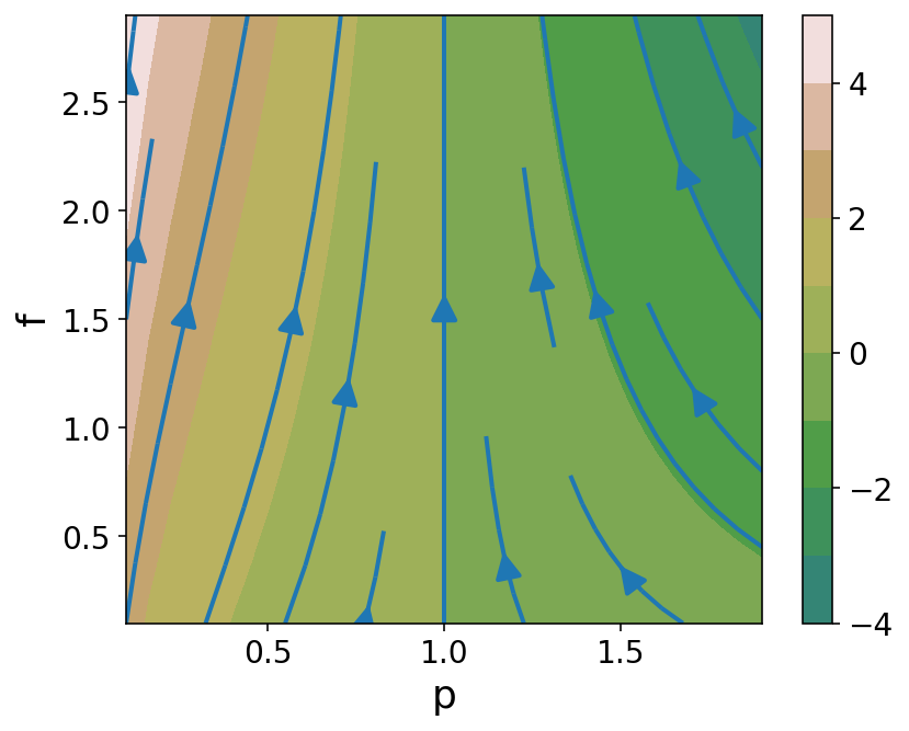
Figure 4: The value (contour colour map) and the generated flows (blue arrow) of the minimum free energy $H(f,P)$ extended to $(0,\infty)\times(0,\infty)$ when $\Theta=\{1\}$. The value and flow at $P=1$ corresponds to that of the minimum free energy in the original domain $(0,\infty)\times\{1\}$.

In the second discrete case $\Theta=\{1,2,3\}$, functions $f$ and probability measures $P$ on $\Theta$ are identified as vectors in the Euclidean space $\mathbb{R}^{3}$. We visualise the first variation $\partial_{1}H(f,P)=P_{*}-P$ and the other first variation $-\partial_{2}H(f,P)=f_{*}+f$ as three-dimensional vectors. Let $f_{0}$ be a function s.t. $(f_{0}(1),f_{0}(2),f_{0}(3))=(2.0,1.0,0.5)$. Figure 5 (b) visualises the first variation $\partial_{1}H(f_{0},P)$ at the fixed $f_{0}$ and each point $P$ in the probability simplex in $\mathbb{R}^{3}$. This illustrates what field on a space of probability measures is induced by the first variation $\partial_{1}H(f_{0},P)$ assigned at every $P$. Let $P_{0}$ be a probability measure s.t. $(P_{0}(1),P_{0}(2),P_{0}(3))=(1/3,1/3,1/3)$. Figure 5 (a) visualises the first variation $-\partial_{2}H(f,P_{0})$ at the fixed $P_{0}$ and each point $f$, again, in the probability simplex in $\mathbb{R}^{3}$. Here, we take each $f$ from the probability simplex for visualisation, but the first variation $-\partial_{2}H(f,P_{0})$ can be defined for all non-negative functions $f$.

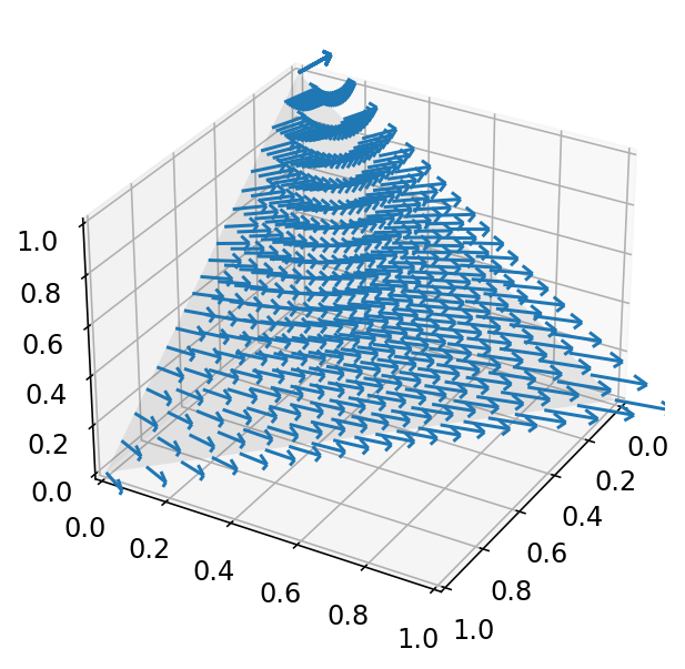
(a) The first variation $-\partial_{2}H(f,P_{0})$

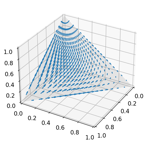
(b) The first variation $\partial_{1}H(f_{0},P)$

Figure 5: The first variations (a) and (b) of the minimum free energy visualised as vectors in $\mathbb{R}^{3}$ when $\Theta=\{1,2,3\}$. With a probability $P_{0}=(1/3,1/3,1/3)$ fixed, the vector (a) is assigned at each $f$ in the simplex s.t. $f(1)+f(2)+f(3)=1$. With a function $f_{0}=(2.0,1.0,0.5)$ fixed, the vector (b) is assigned at each $P$ in the simplex s.t. $P(1)+P(2)+P(3)=1$.

Next, we illustrate an infinite-dimensional flow in the continuous case $\Theta=\mathbb{R}$. We approximate a flow $t\mapsto(f_{t},P_{t})$ from $t=0$ to $t=3$ by the discretisation scheme in (12):

$$(f_{t+\delta},P_{t+\delta})\leftarrow(f_{t},P_{t})+\delta\,\partial H(f_{t},P_{t})$$

where we use $\delta=0.001$. By Theorem 5, the symplectic variation of the minimum free energy at each $(f,P)=(f_{t},P_{t})$ is given by $\partial H(f_{t},P_{t})=(f_{*}+f_{t},P_{*}-P_{t})$ with

$$f_{*}(\theta)=\frac{\exp(-f_{t}(\theta))}{\int_{\Theta}\exp(-f_{t}(\theta))dP_{t}(\theta)}\qquad\text{and}\qquad dP_{*}=\frac{\exp(-f_{t}(\theta))}{\int_{\Theta}\exp(-f_{t}(\theta))dP_{t}(\theta)}dP_{t}(\theta).$$

At any time $t$ in $[0,3]$, the integral $\int_{\Theta}\exp(f_{t}(\theta))dP_{t}(\theta)$ in the definition of $f_{*}$ and $P_{*}$ is numerically computed by the left-endpoint rule using $2000$ grid points over $[-10,10]\subset\Theta$. We identify the measure $P_{t}$ with the density $p_{t}$ with respect to the Lebesgue measure in $\Theta=\mathbb{R}$. We compute the approximated flow $t\mapsto(f_{t},p_{t})$ at each time $t=0,1,2,3$, from two different initial states $(f_{0},p_{0})$. Consider a normal location model $\mathcal{N}(\theta,1)$ over data domain $\mathbb{R}$ with mean parameter $\theta\in\Theta$ and scale $1$. The first initial state $(f_{0},p_{0})$ is defined by the negative log-likelihood $f_{0}(\theta)=(x-\theta)^{2}/2+\log(2\pi)/2$ of the normal location model for datum $x=5.0$ and the density $p_{0}(\theta)=\exp(-\theta^{2}/2)/\sqrt{2\pi}$. Consider a Cauchy location model $\mathcal{C}(\theta,1)$ over data domain $\mathbb{R}$ with mean parameter $\theta\in\Theta$ and scale $1$. The second initial state $(f_{0},p_{0})$ is defined by the negative log-likelihood $f_{0}(\theta)=\log(1+(x-\theta)^{2})+\log(\pi)$ of the Cauchy location model for datum $x=5.0$ and the same density $p_{0}(\theta)=\exp(-\theta^{2}/2)/\sqrt{2\pi}$ as above. Figures 7 and 7 show the approximated flow $t\mapsto(f_{t},P_{t})$ from each initial state.

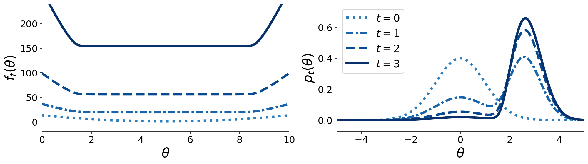
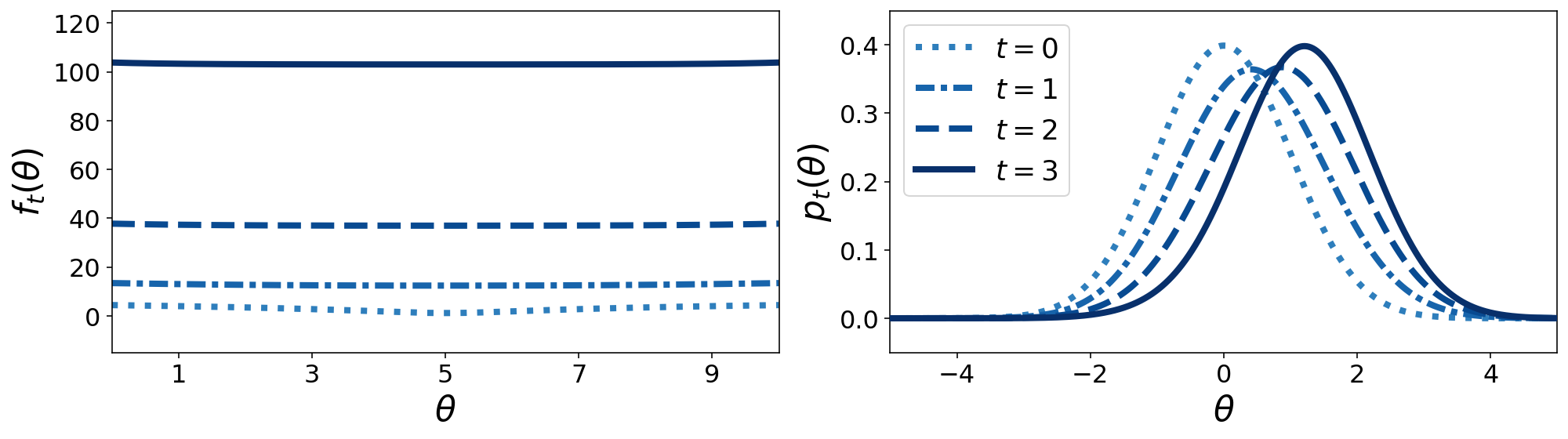
Figure 6: An approximated flow $t\mapsto(f_{t},p_{t})$ of the system of the minimum free energy from an initial state $(f_{0},p_{0})$ given by $f_{0}=(5.0-\theta)^{2}/2+\log(2\pi)/2$ and $p_{0}=\exp(-\theta^{2}/2)/\sqrt{2\pi}$. The left panel shows the evolution of the negative log-likelihood $f_{t}$ and the right panel shows the evolution of the density $p_{t}$, respectively, at time $t=0,1,2,3$.
 

Figure 7: An approximated flow $t\mapsto(f_{t},p_{t})$ of the system of the minimum free energy from an initial state $(f_{0},p_{0})$ given by $f_{0}=\log(1+(5.0-\theta)^{2})+\log(\pi)$ and $p_{0}=\exp(-\theta^{2}/2)/\sqrt{2\pi}$. The left panel shows the evolution of the negative log-likelihood $f_{t}$ and the right panel shows the evolution of the density $p_{t}$, respectively, at time $t=0,1,2,3$.

5 Conclusion

This paper made two theoretical contributions. First, we established the framework of arc Hamiltonian systems for saddle Hamiltonian functions whose domains are infinite-dimensional metric spaces. We derived the general condition, under which a Hamiltonian arc field generates energy-conserving flows everywhere in a metric space. We showed that the general condition reduces to local Lipschitz continuity of the first variation of the Hamiltonian function when the metric on $M$ has an extension to a norm-induced metric on $E_{1}\times E_{2}$. Second, we presented the arc Hamiltonian system of the minimum free energy, in which the difference of the posterior and the prior of Bayesian inference is characterised as the first variation of the minimum free energy $H(f,P)$ with respect to $f$. Pairing this first variation with the other first variation with respect to $P$, we revealed the underlying Hamiltonian arc field behind the transition from the prior and the posterior, as highlighted in Remark 4. The invariance of the conservation of the minimum free energy was established.

In this work, convexity of saddle Hamiltonian functions plays a vital role in the construction of our energy-conserving systems. Arc Hamiltonian systems satisfy the conservation of energy, using only a topologically weak notion of derivative and gradient, i.e., the variational derivative and the first variation. In contrast to the Fréchet derivative, weak notions of derivative, such as the Gâteaux derivative, no longer satisfy the chain rule in general (Yamamuro, 1974). Nonetheless, convexity acts in place of the chain rule to guarantee the energy-conserving property of arc Hamiltonian systems. We focused on saddle Hamiltonian functions that are independent of time $t$. Relaxing time-independence of saddle Hamiltonian functions represents one of natural directions for future work. An extension of arc fields to time-dependent cases was considered in Kim and Masmoudi (2013). In this paper, we applied the framework of arc Hamiltonian systems to formalise the infinite-dimensional geometrical property associated with Bayesian inference. Apart from our application, there may be other intriguing dynamical phenomena or optimisation methodologies that benefit from infinite-dimensional Hamiltonian systems in metric spaces. The general framework of arc Hamiltonian systems can naturally lead to the development of further applications.

Supplementary Material for ‘Hamiltonian Dynamics of Bayesian Inference Formalised by Arc Hamiltonian Systems’ The supplementary material contains proofs for all the theoretical results in the main text.

This supplementary material contains proofs of all the theoretical results presented in the main text. Appendix A provides a concise summary of the theoretical results in Calcaterra and Bleecker (2000) relevant to the theoretical development of arc Hamiltonian systems. It also shows that a part of the original conditions can be relaxed. Appendix B contains proofs of all the theoretical results presented in Section 3. Appendix C contains proofs of all the theoretical results presented in Section 4 apart from the derivation of the first variation. The derivation of the first variation in Section 4 is summarised in Appendix D. Finally, Appendix E presents proofs of three intermediate lemmas used in the proof of Theorem 6.

A The Theory of Arc Fields and The Relaxation of The Condition

Let $(M,d)$ be an arbitrary complete metric space and let $\Phi:M\times[0,1]\to M$ be an arbitrary map s.t. $\Phi_{0}(x)=x$ throughout Appendix A. Recall that the map $\Phi$ is called an arc field if it satisfies the condition in Definition 1. Calcaterra and Bleecker (2000) were concerned with a curve $t\mapsto x_{t}$ in $(M,d)$ that satisfies the following condition at each time $t$:

$$\lim_{s\to 0^{+}}\frac{d(x_{t+s},\Phi_{s}(x_{t}))}{s}=0.$$ (S1)

They established conditions for the map $\Phi$, under which a unique solution $t\mapsto x_{t}$ of (S1) from $x_{0}=a$ exists in the infinite interval $[0,\infty)$ for every starting point $a\in M$.

In Section A.1, we provide a brief recap of their results relevant to the theoretical development of arc Hamiltonian systems. We restate their results using our notation, remarking corresponding statements of Calcaterra and Bleecker (2000) in each statement provided in Section A.1. We prefix ‘CB-’ to statements of Calcaterra and Bleecker (2000) refered here—e.g., CB-Definition 2.1—for simpler citation. In Section A.2, we show that a part of their original conditions can be relaxed. Section A.3 contains the proof of the relaxation.

A.1 The Theory of Arc Fields

First, they studied under what condition a unique solution $t\mapsto x_{t}$ of (S1) exists at least in some finite interval $[0,T)$ at each starting point. They provided the following two fundamental conditions.

Assumption 9 (CB-Condition AL).

For some function $\Lambda:M\times M\times[0,1]\to\mathbb{R}$, at each $a\in M$ there exist a radius $r_{a}>0$ and a length $\epsilon_{a}>0$ s.t.

$$d(\Phi_{t}(x),\Phi_{t}(v))\leq d(x,v)(1+t\,\Lambda(x,v,t))$$

and $\Lambda(x,v,t)$ is upper bounded for all $x,v\in B_{r_{a}}(a)$ and $t\in[0,\epsilon_{a})$.

Assumption 10 (CB-Condition BL).

For some function $\Omega:M\times[0,1]\times[0,1]\to[0,\infty)$, at each $a\in M$ there exist a radius $r_{a}>0$ and a length $\epsilon_{a}>0$ s.t.

$$d(\Phi_{t+s}(x),\Phi_{s}(\Phi_{t}(x)))\leq t\,s\,\Omega(x,t,s))$$

and $\Omega(x,t,s))$ is upper bounded for all $x\in B_{r_{a}}(a)$ and $t,s\in[0,\epsilon_{a})$.

Originally, the above inequality in CB-Condition BL was stated in a form

$$d(\Phi_{t+s}(x),\Phi_{s}(\Phi_{t}(x)))\leq t\,g(t,s)\,\Omega(x,t,s))$$

using some function $g:[0,\epsilon_{a})\times[0,\epsilon_{a})\to[0,\infty)$. However, CB-Remark 2.1 highlighted that it suffices to set $g(t,s)=s$ in CB-Condition BL. We hence use $g(t,s)=s$ as our default choice in 10 by combining CB-Condition BL and CB-Remark 2.1.

By CB-Definition 4.1, an arc field $\Phi$ is said to have unique solutions for short time if there exists an interval $[0,T_{a})$ at each point $a\in M$, in which a unique solution $t\mapsto x_{t}$ of (S1) exists from $x_{0}=a$. This means that, if two non-unique solutions of (S1) exist from $x_{0}=a$ in some interval larger than $[0,T_{a})$, they must equal to each other at least in the interval $[0,T_{a})$. Then they showed in CB-Proposition 4.2 that, if an arc field $\Phi$ has unique solutions for short time, a maximal solution (i.e. the longest solution that can exist) at each point is, in fact, unique. In other words, any solution of (S1), shown to exists in some interval, turns out to be a part of the underlying longest unique solution. CB-Proposition 4.2 formalised this intuition.

Proposition 4 (CB-Proposition 4.2).

Assume that an arc field $\Phi$ has unique solutions for short time. At each point $a\in M$, there exists a unique solution $t\mapsto x_{t}$ of (S1) from $x_{0}=a$ in some interval $[0,T_{a}^{*})$ s.t. for any solution $t\mapsto\hat{x}_{t}$ of (S1) from $\hat{x}_{0}=a$ whose interval is $[0,T_{a})$, we have $T_{a}^{*}\geq T_{a}$ and $t\mapsto\hat{x}_{t}$ equals to $t\mapsto x_{t}$ everywhere in $[0,T_{a})$.

They concisely summarised in CB-Corollary 4.3 that an arc field $\Phi$ has unique solutions for short time under CB-Condition AL and CB-Condition BL.

Corollary 1 (CB-Corollary 4.3).

An arc field $\Phi$ that satisfies Assumptions 9–10 has unique solutions for short time, and hence has a unique maximal solution of (S1) starting from each point in $M$.

In CB-Corollary 4.3, the interval in which each unique maximal solution exists was implicit. They next studied under what additional condition each unique maximal solution exists globally in the infinite interval $[0,\infty)$. For simplicity, we drop the term ‘maximal’ for any unique solution in $[0,\infty)$, because a unique solution in $[0,\infty)$ is trivially the longest solution. They used a condition, termed linear speed growth, and showed the existence of a unique solution in the infinite interval $[0,\infty)$ in CB-Theorem 4.4.

Definition 8 (CB-Definition 4.2).

An arc field $\Phi$ is said to have linear speed growth if there exists a point $x\in M$ and some constant $C_{1},C_{2}$ dependent only on $x$ s.t.

$$\bar{\rho}(x,r)\leq C_{1}\,r+C_{2}$$

holds for all $r>0$, where $\bar{\rho}$ is defined in Definition 1.

Theorem 7 (CB-Theorem 4.4).

Assume that an arc field $\Phi$ satisfies Assumptions 9–10 and has linear speed growth. At each $a\in M$, there exists a unique solution $t\mapsto x_{t}$ of (S1) from $x_{0}=a$ in $[0,\infty)$.

Note that each unique solution above is continuous while this was implicit in CB-Theorem 4.4. Continuity of each solution is made explicit in our statement in Section A.2. We move on to Section A.2, where we weaken CB-Definition 4.2 and reproduce CB-Theorem 4.4.

A.2 The Relaxation of The Condition

The condition of CB-Definition 4.2 for an arc field $\Phi$ requires that the inequality $\bar{\rho}(x,r)\leq C_{1}\,r+C_{2}$ holds for all radius $r$ in $(0,\infty)$. This is in contrast to the inequalities in Assumptions 9–10 that need to hold only for all radius $r$ smaller than some constant $r_{a}$ at each point $a\in M$. The condition of CB-Definition 4.2 may be restrictive for some application; in the theory of arc Hamiltonian systems, we use local Lipschitz continuity of the first variation of a Hamiltonian function to show the existence of a flow. We conclude Appendix A by showing that the condition of CB-Definition 4.2 can be relaxed in a manner that an analogous inequality holds only for all radius $r$ smaller than some constant $r_{a}$ at each point $a\in M$. The function $\rho$ in 11 is defined in Definition 1.

Assumption 11.

At each $a\in M$, there exist a radius $r_{a}>0$ s.t.

$$\rho(a)\leq C_{1}d(x,a)+C_{2}$$

holds for all $x\in B_{r_{a}}(a)$, where $C_{1},C_{2}$ are constants dependent only on $a$.

Here, we note that a map $\Phi$ that satisfies 11 is in fact an arc field.

Lemma 1.

A map $\Phi$ that satisfies 11 is an arc field on $(M,d)$.

Proof.

Recall from Definition 1 that $\bar{\rho}(x,r)=\sup_{v\in B_{r}(x)}\rho(v)$. It follows from 11 that each $a\in M$ there exist a radius $r_{a}>0$ s.t. it holds for all $0<r\leq r_{a}$ that

$$\bar{\rho}(a,r)=\sup_{v\in B_{r}(a)}\rho(v)\leq\sup_{v\in B_{r}(a)}\left(C_{1}d(v,a)+C_{2}\right)\leq C_{1}\,r_{a}+C_{2}$$

where the last inequality is immediate from $v\in B_{r}(a)$ and $r\leq r_{a}$. Since $\bar{\rho}(a,r)<\infty$ for all $0<r\leq r_{a}$ at each $a\in M$, we conclude that $\Phi$ satisfies Definition 1 and is an arc field. ∎

Now, we reproduce CB-Theorem 4.4 under 11 without using the condition of CB-Definition 4.2. Continuity of each solution is made explicit in the following Theorem 8.

Theorem 8.

Suppose that a map $\Phi$ satisfies Assumptions 9–11. At each $a\in M$, there exists a unique continuous solution $t\mapsto x_{t}$ of (S1) from $x_{0}=a$ in $[0,\infty)$.

The proof of Theorem 8 is provided in Section A.3. Theorem 8 is the main result that directly used in the theoretical development of arc Hamiltonian systems. This completes the brief recap of the theory of arc fields and the relaxation of the condition.

A.3 Proof of Theorem 8

We introduce an intermediate lemma used in the main proof.

Lemma 2.

Suppose that for a point $a\in M$ an arc field $\Phi$ has a unique solution $t\mapsto x_{t}$ from $x_{0}=a$ in some interval. Given any radius $r>0$, there exists some length $T_{a}>0$ s.t. the unique solution $t\mapsto x_{t}$ from $x_{0}=a$ satisfies $x_{t}\in B_{r}(a)$ for all $t\in[0,T_{a})$.

Proof of Lemma 2.

Denote by $[0,T_{a}^{*})$ the interval in which a unique solution $t\mapsto x_{t}$ from $x_{0}=a$ is supposed to exist. Let $t$ be an arbitrary point in $[0,T_{a}^{*})$ and let $s$ be any variable in $[0,T_{a}^{*}-t)$, where we have $0\leq t+s<T_{a}^{*}$. By the triangle inequality, we have

$$d(x_{t+s},x_{t}) \leq d(x_{t+s},\Phi_{s}(x_{t}))+d(\Phi_{s}(x_{t}),x_{t})$$

$$=d(x_{t+s},\Phi_{s}(x_{t}))+d(\Phi_{s}(x_{t}),\Phi_{0}(x_{t}))$$

$$=s\cdot\frac{d(x_{t+s},\Phi_{s}(x_{t}))}{s}+s\cdot\frac{d(\Phi_{s}(x_{t}),\Phi_{0}(x_{t}))}{s}.$$

In the above inequality, we plug the following trivial inequality

$$\frac{d(\Phi_{s}(x_{t}),\Phi_{0}(x_{t}))}{s}\leq\sup_{s_{1}\neq s_{2}\in[0,1]}\frac{d(\Phi_{s_{1}}(x_{t}),\Phi_{s_{2}}(x_{t}))}{|s_{1}-s_{2}|}=\rho(x_{t})$$

where $\rho$ is the function defined in Definition 1. We take the limit $s\to 0^{+}$ to see that

$$\lim_{s\to 0^{+}}d(x_{t+s},x_{t}) =\lim_{s\to 0^{+}}\left(s\cdot\frac{d(x_{t+s},\Phi_{s}(x_{t}))}{s}+s\cdot\rho(x_{t})\right)$$

$$=\underbrace{\lim_{s\to 0^{+}}s}_{=0}\cdot\underbrace{\lim_{s\to 0^{+}}\frac{d(x_{t+s},\Phi_{s}(x_{t}))}{s}}_{=:(*)}+\underbrace{\lim_{s\to 0^{+}}s}_{=0}\cdot\underbrace{\vphantom{\lim_{s\to 0^{+}}}\rho(x_{t})}_{<\infty}.$$

We have $(*)=0$ by the condition (S1) and have $\rho(x_{t})<\infty$ by Definition 1. We set $t=0$ to see that $\lim_{s\to 0^{+}}d(x_{s},x_{0})=\lim_{s\to 0^{+}}d(x_{s},a)=0$. By definition of convergence, for any value $r>0$, we can take some value $T_{a}>0$ so that $d(x_{s},a)<r$ holds for all $s\in[0,T_{a})$. ∎

Now, we present the main proof of Theorem 8.

Proof of Theorem 1.

By Lemma 1, the map $\Phi$ is an arc field under 11. Let $a$ be an arbitrary point in $M$. Let $r_{a}>0$ be the radius that the inequality in 11 holds at $a\in M$. By Corollary 1, the arc field $\Phi$ has unique solutions for short time. Hence a unique solution $t\mapsto x_{t}$ from $x_{0}=a$ exists in some interval. By Lemma 2, there exists some $T_{a}>0$ s.t. the solution $t\mapsto x_{t}$ from $x_{0}=a$ satisfies $x_{t}\in B_{r_{a}}(a)$ for all $t\in[0,T_{a})$.

Our aim is to show that the unique solution $t\mapsto x_{t}$ in $[0,T_{a})$ can be uniquely and indefinitely extended to $[0,\infty)$, by the same argument in the proof of CB-Theorem 4.4. Let $\{t_{n}\}_{n=1}^{\infty}$ be a Cauchy sequence in $[0,T_{a})$ s.t. $t_{n}\to T_{a}$. A key part of the proof is to show that

$(\star)$ the solution sequence $\{x_{t_{n}}\}_{n=1}^{\infty}$ from $x_{t_{1}}=a$ is Cauchy.

If item $(\star)$ holds, the solution $t\mapsto x_{t}$ from $x_{0}=a$ converges to some point $b\in M$ as $t\to T_{a}$. This implies that, at $t=T_{a}$, the solution $t\mapsto x_{t}$ connects to the other unique solution $t\mapsto\hat{x}_{t}$ running from $\hat{x}_{0}=b$ in some interval $[0,T_{b})$. Since we show item $(\star)$ for arbitrary $a$, the other solution $t\mapsto\hat{x}_{t}$ from $b$ is also Cauchy and converges to some point $c\in M$ as $t\to T_{b}$. By repeating this process, the original solution from $a$ can be continued over $[0,\infty)$. By Proposition 4, the continued solution in $[0,\infty)$ is unique, which concludes the existence of a unique solution in $[0,\infty)$. Continuity of the solution is clarified in the end of this proof.

It suffices to prove item $(\star)$. We repeat the argument in the proof of CB-Theorem 4.4 for item $(\star)$, using only 11. Let $f(t):=d(x_{t},x_{0})$ for any $t\in[0,T_{a})$ where $x_{0}=a$. For any $t\in[0,T_{a})$ and $h\in[0,T_{a}-t)$, it follows from the reverse triangle inequality that

$$f(t+h)-f(t)=d(x_{t+h},x_{0})-d(x_{t},x_{0})\leq d(x_{t+h},x_{t}).$$

It further follows from the triangle inequality that

$$f(t+h)-f(t) \leq d(x_{t+h},\Phi_{h}(x_{t}))+d(\Phi_{h}(x_{t}),x_{t})$$

$$=d(x_{t+h},\Phi_{h}(x_{t}))+h\cdot\frac{d(\Phi_{h}(x_{t}),\Phi_{0}(x_{t}))}{h}$$

$$\leq d(x_{t+h},\Phi_{h}(x_{t}))+h\cdot\rho(x_{t}).$$

Dividing both the side by $h$ and taking the limit in $h\to 0^{+}$, we have

$$\lim_{h\to 0^{+}}\frac{f(t+h)-f(t)}{h} \leq\lim_{h\to 0^{+}}\frac{d(x_{t+h},\Phi_{h}(x_{t}))}{h}+\rho(x_{t})=\rho(x_{t}).$$

where $\lim_{h\to 0^{+}}d(x_{t+h},\Phi_{h}(x_{t}))/h=0$ due to the condition (S1). Recall that $x_{t}\in B_{r_{a}}(x_{0})$ holds for all $t\in[0,T_{a})$, where $x_{0}=a$. Since $r_{a}$ is the radius under which the inequality in 11 holds at $a$, we can apply the inequality of $\rho(x_{t})$ for all $t\in[0,T_{a})$, that is,

$$\lim_{h\to 0^{+}}\frac{f(t+h)-f(t)}{h} \leq C_{1}d(x_{t},x_{0})+C_{2}=C_{1}f(t)+C_{2}.$$ (S2)

This inequality (S2) implies a bound $f(t)\leq(C_{2}/C_{1})(\exp(C_{1}t)-1)$. To verify this, we set $g(t):=\exp(-C_{1}t)(f(t)+C_{2}/C_{1})$ and calculate its right-derivative

$$\lim_{h\to 0^{+}}\frac{g(t+h)-g(t)}{h} =\exp(-C_{1}t)\left(\lim_{h\to 0^{+}}\frac{f(t+h)-f(t)}{h}-C_{1}f(t)-C_{2}\right)\leq 0$$

where the right-hand side is non-positive because of the inequality (S2). Since the right-derivative is non-positive, $g$ decreases over $[0,T_{*})$ and hence $g(t)\leq g(0)$, which leads to

$$g(t)=\exp(-C_{1}t)\left(f(t)+\frac{C_{2}}{C_{1}}\right)\leq\frac{C_{2}}{C_{1}}=g(0)$$

where we used $f(0)=0$. Rearranging the term confirms that we have the intended bound $f(t)\leq(C_{2}/C_{1})(\exp(C_{1}t)-1)$. Since $f(t)=d(x_{t},x_{0})$, we arrive at a main bound:

$$d(x_{t},x_{0})\leq\frac{C_{2}}{C_{1}}(\exp(C_{1}t)-1).$$ (S3)

Let $s$ be an arbitrary point in $[0,T_{a})$. Define $v_{t}:=x_{s+t}$ for any $t\in[0,T_{*}-s)$, where $v_{0}=x_{s}$. We aim to derive an upper bound of $d(v_{t},v_{0})$ similar to (S3). The above argument for $f(t)=d(x_{t},x_{0})$ depends only on the condition $\rho(x_{t})\leq C_{1}d(x_{t},x_{0})+C_{2}$. If a corresponding condition $\rho(v_{t})\leq C_{1}^{\prime}d(v_{t},v_{0})+C_{2}^{\prime}$ holds for some constants $C_{1}^{\prime}$ and $C_{2}^{\prime}$, we have

$$d(v_{t},v_{0})\leq\frac{C_{2}^{\prime}}{C_{1}^{\prime}}(\exp(C_{1}^{\prime}t)-1).$$ (S4)

In fact, the required condition holds for $C_{1}^{\prime}=C_{1}$ and $C_{2}^{\prime}=C_{1}d(x_{s},x_{0})+C_{2}$ because

$$\rho(x_{s+t})\leq C_{1}\,d(x_{s+t},x_{0})+C_{2}\leq C_{1}\,d(x_{s+t},x_{s})+C_{1}\,d(x_{s},x_{0})+C_{2}$$

where the first inequality follows from the inequality in 11 and the last inequaliy follows from the triangle inequality. Applying (S3) for $d(x_{s},x_{0})$ in the constant $C_{2}^{\prime}$, we further have $C_{2}^{\prime}\leq C_{2}\exp(C_{1}T_{a})$. We plug these constants $C_{1}^{\prime}$ and $C_{2}^{\prime}$ in (S4) to see that

$$d(x_{s+t},x_{s}) \leq\frac{C_{2}\exp(C_{1}T_{a})}{C_{1}}|\exp(C_{1}t)-\exp(0)|.$$

Since the mean value theorem implies $|\exp(C_{1}t)-\exp(0)|\leq\exp(C_{1}T_{a})|C_{1}t-0|$ for any $t\in[0,T_{a})$, we have, for arbitrary $s\in[0,T_{a})$ and $t\in[0,T_{a}-s)$, that

$$d(x_{s+t},x_{s}) \leq C_{2}\exp(2C_{1}T_{a})\,|t|.$$

Since the metric $d$ are symmetric, we can rewrite this inequality as

$$d(x_{t},x_{s}) \leq C_{2}\exp(2C_{1}T_{a})\,|t-s|$$ (S5)

for any $s,t\in[0,T_{a})$. This inequality implies Lipschitz continuity of the solution $t\mapsto x_{t}$ in $[0,T_{a})$. We conclude that the solution sequence $\{x_{t_{n}}\}_{n=1}^{\infty}$ is Cauchy as intended, because we have $d(x_{t_{n}},x_{t_{m}})\to 0$ whenever $|t_{n}-t_{m}|\to 0$ due to (S5).

Finally, we make explicit continuity of the continued solution in $[0,\infty)$. As aforementioned, a solution $t\mapsto x_{t}$ from $x_{0}=a$ in $[0,T_{a})$ converges to some point $b\in M$ at $t=T_{a}$ and connects to the other solution $t\mapsto\hat{x}_{t}$ from $\hat{x}_{0}=b$ in $[0,T_{b})$. Since $a$ is arbitrary in this proof, both the solution $t\mapsto x_{t}$ from $x_{0}=a$ and the solution $t\mapsto\hat{x}_{t}$ from $\hat{x}_{0}=b$ satisfy Lipschitz continuity (S5). Thus, the connected solution over $[0,T_{a}+T_{b})$ is continuous if it is continuous at $b$. It is trivially continuous at $b$ since the two solutions are concatenated at $b$. By repeating this process, the solution $t\mapsto x_{t}$ from $a$ continues over $[0,\infty)$ continuously. ∎

B Proofs for Results in Section 3

B.1 Proof of Theorem 1

Theorem 4.4 of Calcaterra and Bleecker (2000) established conditions for an arbitrary arc field $\Phi:M\times[0,1]\to M$, under which a unique solution of the associated condition (6) exists in $[0,\infty)$ from any initial point in $M$. See Section A.1 for a summary of their results. We established in Theorem 8 in Section A.2 that a part of their original assumptions can be relaxed. Theorem 1 is a direct application of Theorem 8 stated under the relaxed assumptions suitable for our theoretical development.

Proof.

By definition, a global flow of the system from a point $(x,z)$ is a unique continuous solution $t\mapsto(x_{t},z_{t})$ of the arc Hamilton equation (11) from $(x_{0},z_{0})=(x,z)$ in the infinite interval $[0,\infty)$. Theorem 8 shows that a unique continuous solution of the condition (6) exists in the infinite interval $[0,\infty)$ from every initial point in $M$ if the associated map $\Phi$ satisfies Assumptions 9–11. For the arc Hamilton equation (11), 1 restates Assumptions 9–10 combined together and 2 restates 11. ∎

B.2 Proof of Theorem 2

In Section B.2, let $\|\cdot\|_{E}$ be the norm on $E=E_{1}\times E_{2}$ that induces the metric $d_{*}$ on $E$ in 3 item (1). Since $d_{*}$ is an extension of $d$ from $M$ to $E$, we have $d((x,z),(v,y))=d_{*}((x,z),(v,y))=\|(x,z)-(v,y)\|_{E}$ everywhere in $M$. We introduce an intermediate lemma used in the main proof.

Lemma 3.

Suppose 3. For any $(x,z)\in M$, we have

$$d((x,z),\Phi_{s}(x,z))=s\|\partial H(x,z)\|_{E}.$$

At each $(x_{0},z_{0})\in M$, it holds for all $(x,z)\in B_{\delta_{0}}(x_{0},z_{0})$ that

$$\|\partial H(x,z)\|_{E}\leq K_{0}\,d((x,z),(x_{0},z_{0}))+\|\partial H(x_{0},z_{0})\|_{E}$$

where $\delta_{0}$ is the radius and $K_{0}$ is the constant of local Lipshitz continuity (13) at $(x_{0},z_{0})$.

Proof of Lemma 3.

The first equality is immediate from

$$d((x,z),\Phi_{s}(x,z)) =\|(x,z)-(x,z)-s\,\partial H(x,z))\|_{E}=s\|\partial H(x,z)\|_{E}.$$

For any $(x,z)\in B_{\delta_{0}}(x_{0},z_{0})$, we apply the triangle inequality to see that

$$\|\partial H(x,z)\|_{E} \leq\|\partial H(x,z)-\partial H(x_{0},z_{0})\|_{E}+\|\partial H(x_{0},z_{0})\|_{E}$$

$$=d_{*}(\partial H(x,z),\partial H(x_{0},z_{0}))+\|\partial H(x_{0},z_{0})\|_{E}$$

$$\leq K_{0}\,d((x,z),(x_{0},z_{0}))+\|\partial H(x_{0},z_{0})\|_{E}$$

where the last inequality follows from local Lipschitz continuity (13). ∎

Now, we provide the main proof of Theorem 2.

Proof of Theorem 2.

First, we specify the functions $\Lambda:M\times M\times[0,1]\to\mathbb{R}$ and $\Omega:M\times[0,1]\times[0,1]\to[0,\infty)$, for which 1 is shown to hold:

$$\Lambda((x,z),(v,y),t) =\frac{d_{*}(\partial H(x,z),\partial H(v,y))}{d((x,z),(v,y))},$$

$$\Omega((x,z),t,s) =\Lambda((x,z),\Phi_{s}(x,z),t)\|\partial H(x,z)\|_{E}.$$

Here, we verify $\Lambda$ and $\Omega$ are well-defined at each point. If $(x,z)\neq(v,y)$, the value of $\Lambda$ at each point is finite because $d((x,z),(v,y))\neq 0$. Even if $(x,z)=(v,y)$, the value of $\Lambda$ is finite because local Lipschitz continuity (13) implies that, for all $(x,z),(v,y)\in B_{\delta_{0}}(x_{0},z_{0})$,

$$\Lambda((x,z),(v,y),t)\leq\frac{K_{0}\,d((x,z),(v,y))}{d((x,z),(v,y))}=K_{0}$$ (S6)

at each point $(x_{0},z_{0})\in M$. Therefore, $\Lambda$ is well-defined at each point, so does $\Omega$.

In what follows, let $(x_{0},z_{0})$ be an arbitrary point in $M$. Let $\delta_{0}>0$ be the radius that local Lipschitz continuity (13) in 3 holds at $(x_{0},z_{0})$. Let $(x,z),(v,y)$ be arbitrary points in an open ball $B_{r_{0}}(x_{0},z_{0})$ for a given radius $r_{0}\in(0,\infty)$. Let $t,s$ be arbitrary points in an interval $[0,\epsilon_{0})$ for a given length $\epsilon_{0}\in(0,1]$. First, we show that there exist some radius $r_{0}>0$ and length $\epsilon_{0}>0$ s.t. 1 items (1)–(2) hold.

1 item (1): It follows from the triangle inequality that

$$d(\Phi_{t}(x,z),\Phi_{t}(v,y)) =\|(x,z)+t\partial H(x,z)-(v,y)-t\partial H(v,y)\|_{E}$$

$$\leq\|(x,z)-(v,y)\|_{E}+\|t\partial H(x,z)-t\partial H(v,y)\|_{E}$$

$$=d_{*}((x,z),(v,y))+td_{*}(\partial H(x,z),\partial H(v,y)).$$

Since $d_{*}((x,z),(v,y))=d((x,z),(v,y))$ everywhere in $M$, we have

$$d(\Phi_{t}(x,z),\Phi_{t}(v,y)) \leq d((x,z),(v,y))+t\,d_{*}(\partial H(x,z),\partial H(v,y))$$

$$=d((x,z),(v,y))\,\left(1+t\,\Lambda((x,z),(v,y),t)\right).$$

If $(x,z),(v,y)$ are contained in $B_{\delta_{0}}(x_{0},z_{0})$, the term $\Lambda((x,z),(v,y),t)$ is bounded by $K_{0}$ as established in (S6). Selecting any $r_{0}\leq\delta_{0}$ and $\epsilon_{0}\in(0,1]$ concludes 1 item (1).

1 item (2): Denote $(\tilde{x}_{s},\tilde{z}_{s}):=\Phi_{s}(x,z)=(x,z)+s\,\partial H(x,z)$ to see

$$d(\Phi_{t+s}(x,z),\Phi_{t}(\Phi_{s}(x,z))) =\|(x,z)+(t+s)\,\partial H(x,z)-(\tilde{x}_{s},\tilde{z}_{s})-t\,\partial H(\tilde{x}_{s},\tilde{z}_{s})\|_{E}$$

$$=\|(\tilde{x}_{s},\tilde{z}_{s})+t\,\partial H(x,z)-(\tilde{x}_{s},\tilde{z}_{s})-t\,\partial H(\tilde{x}_{s},\tilde{z}_{s})\|_{E}$$

$$=t~{}d_{*}(\partial H(x,z),\partial H(\tilde{x}_{s},\tilde{z}_{s}))$$

$$=t~{}\Lambda((x,z),(\tilde{x}_{s},\tilde{z}_{s}),t)~{}d((x,z),(\tilde{x}_{s},\tilde{z}_{s})).$$

Since $d((x,z),(\tilde{x}_{s},\tilde{z}_{s}))=s\|\partial H(x,z)\|_{E}$ by Lemma 3, it follows from definition of $\Omega$ that

$$d(\Phi_{t+s}(x,z),\Phi_{t}(\Phi_{s}(x,z))) =t\,s\,\Omega((x,z),s,t).$$

We can conclude 1 item (2) if there exist some $r_{0}>0$ and $\epsilon_{0}>0$ s.t. $\Omega((x,z),s,t)$ is bounded for all $(x,z)\in B_{r_{0}}(x_{0},z_{0})$ and all $s,t\in[0,\epsilon_{0})$. Since by definition we have $\Omega((x,z),t,s)=\Lambda((x,z),\Phi_{s}(x,z),t)\|\partial H(x,z)\|_{E}$, we will upper bound each component $\Lambda((x,z),\Phi_{s}(x,z),t)$ and $\|\partial H(x,z)\|_{E}$. If we have $(x,z)\in B_{\delta_{0}}(x_{0},z_{0})$, Lemma 3 shows that $\|\partial H(x,z)\|_{E}\leq Kr_{0}+\|\partial H(x_{0},z_{0})\|_{E}<\infty$. It thus suffices to take any $r_{0}\leq\delta_{0}$ to upper bound the second component. It is established in (S6) that $\Lambda((x,z),\Phi_{s}(x,z),t)\leq K_{0}$ if both $(x,z)$ and $\Phi_{s}(x,z)$ are contained in $B_{\delta_{0}}(x_{0},z_{0})$. In fact, if we have $(x,z)\in B_{\delta_{0}/2}(x_{0},z_{0})$, there exists $\epsilon_{0}>0$ s.t. $\Phi_{s}(x,z)\in B_{\delta_{0}}(x_{0},z_{0})$ for all $s\in[0,\epsilon_{0})$. To verify this, see that Lemma 3 implies $\lim_{s\to 0^{+}}d((x,z),\Phi_{s}(x,z))=0$. By definition of convergence, for any given $r>0$ there exists some $\epsilon_{r}>0$ s.t. $d((x,z),\Phi_{s}(x,z))<r$ for all $s\in[0,\epsilon_{r})$. That is, given the radius $\delta_{0}/2$, there exists some $\epsilon_{*}>0$ s.t. $\Phi_{s}(x,z)$ is contained in $B_{\delta_{0}/2}(x,z)$ for all $s\in[0,\epsilon_{*})$. Clearly, the open ball $B_{\delta_{0}/2}(x,z)$ around $(x,z)$ is further contained in the open ball $B_{\delta_{0}}(x_{0},z_{0})$ around $(x_{0},z_{0})$ if we have $(x,z)\in B_{\delta_{0}/2}(x_{0},z_{0})$. This means that, if we take any $r_{0}\leq\delta_{0}/2$, then $(x,z)$ and $\Phi_{s}(x,z)$ are both contained in $B_{\delta_{0}}(x_{0},z_{0})$ for all $s\in[0,\epsilon_{*})$. Therefore, selecting any $r_{0}\leq\delta_{0}/2$ and $\epsilon_{0}\leq\epsilon_{*}$ guarantees that $\Omega((x,z),s,t)$ is bounded.

We complete the proof by showing 2.

2: Since $d(\Phi_{t}(x,z),\Phi_{s}(x,z))=\|\Phi_{t}(x,z)-\Phi_{s}(x,z)\|_{E}$, we have

$$\rho(x,z) =\sup_{t\neq s\in[0,1]}\frac{\|(x,z)+t\,\partial H(x,z)-(x,z)-s\,\partial H(x,z)\|_{E}}{|t-s|}=\|\partial H(x,z)\|_{E}.$$

By selecting any $r_{0}\leq\delta_{0}$ so that $(x,z)\in B_{\delta_{0}}(x_{0},z_{0})$, it follows from Lemma 3 that

$$\rho(x,z) =\|\partial H(x,z)\|_{E}\leq K_{0}\,d((x,z),(x_{0},z_{0}))+\|\partial H(x_{0},z_{0})\|_{E}.$$ (S7)

Setting $C_{1}=K_{0}$ and $C_{2}=\|\partial H(x_{0},z_{0})\|_{E}$ concludes 2. ∎

B.3 Proof of Theorem 3

If a convex function $f:E_{1}\to\overline{\mathbb{R}}$ admits the first variation $\partial f(x)\in E_{2}$ at $x\in\operatorname{Dom}(f)$, the following inequality holds for any $v\in\operatorname{Dom}(f)$:

$$\langle v-x,\partial f(x)\rangle=\lim_{\epsilon\to 0^{+}}\frac{f((1-\epsilon)x+\epsilon v)-f(x)}{\epsilon}\leq f(v)-f(x).$$ (S8)

The first equality follows from definition of the first variation, where $v-x$ is a trivial element of $C(x)$. The last inequality follows from convexity $f((1-\epsilon)x+\epsilon v)\leq(1-\epsilon)f(x)+\epsilon f(v)$. If $f:E_{1}\to\overline{\mathbb{R}}$ is a concave function, we have the inequality with the less-than sign flipped

$$\langle v-x,\partial f(x)\rangle\geq f(v)-f(x).$$ (S9)

Note that the essentially same inequalities hold for a convex or concave function in $E_{2}$. We introduce a lemma that applies (S8) and (S9) for a saddle function $H:E_{1}\times E_{2}\to\overline{\mathbb{R}}$.

Lemma 4.

Suppose that a saddle function $H:E_{1}\times E_{2}\to\overline{\mathbb{R}}$ has the first variations $\partial_{1}H(x,z)$ and $\partial_{2}H(x,z)$ everywhere in $\operatorname{Dom}(H)$. For any $(x,z),(v,y)\in\operatorname{Dom}(H)$,

$$H(v,y)-H(x,z) \geq\langle v-x,\partial_{1}H(v,y)\rangle+\langle\partial_{2}H(x,z),y-z\rangle,$$

$$H(v,y)-H(x,z) \leq\langle v-x,\partial_{1}H(x,y)\rangle+\langle\partial_{2}H(x,y),y-z\rangle.$$

Proof of Lemma 4.

Let $(x,z),(v,y)$ be arbitrary points in $\operatorname{Dom}(H)$. Denote $H_{y}(\cdot):=H(\cdot,y)$ for fixed $y$ and $H_{x}(\cdot):=H(x,\cdot)$ for fixed $x$, where $H_{y}$ is concave and $H_{x}$ is convex. By definition, the first variation of $H_{y}$ at $x$ is $\partial_{1}H(x,y)$, and the first variation of $H_{x}$ at $z$ is $\partial_{2}H(v,z)$. We apply (S9) for both (i) $H_{y}(v)-H_{y}(x)$ and (ii) $H_{y}(x)-H_{y}(v)$ to see that

(i) $$\langle v-x,\partial_{1}H(x,y)\rangle\geq H_{y}(v)-H_{y}(x),$$

(ii) $$\langle x-v,\partial_{1}H(v,y)\rangle\geq H_{y}(x)-H_{y}(v).$$

We multiply both sides of the inequality (ii) by $-1$ to have that

$$\langle v-x,\partial_{1}H(v,y)\rangle\leq H_{y}(v)-H_{y}(x)\leq\langle v-x,\partial_{1}H(x,y)\rangle.$$ (S10)

Similarly, we apply (S8) for both (iii) $H_{x}(y)-H_{x}(z)$ and (iv) $H_{x}(z)-H_{x}(y)$ to see that

(iii) $$\langle\partial_{2}H(x,z),y-z\rangle\leq H_{x}(y)-H_{x}(z),$$

(iv) $$\langle\partial_{2}H(x,y),z-y\rangle\leq H_{x}(z)-H_{x}(y).$$

We multiply both sides of the inequality (iv) by $-1$ to have that

$$\langle\partial_{2}H(x,z),y-z\rangle\leq H_{x}(y)-H_{x}(z)\leq\langle\partial_{2}H(x,y),y-z\rangle.$$ (S11)

Adding all sides of (S10) and (S11) completes the proof. ∎

Now we present the main proof of Theorem 3.

Proof of Theorem 3.

It suffices to show that (i) $t\mapsto H(x_{t},z_{t})$ is continuous in $[0,T)$ and (ii) the right derivative $(d^{+}/dt)H(x_{t},z_{t})$ equals to zero everywhere in $[0,T)$. First of all, item (i) immediately holds by combining local Lipschitz continuity (14)

$$|H(x_{s},z_{s})-H(x_{t},z_{t})|\leq J_{0}\,d((x_{s},z_{s}),(x_{t},z_{t}))$$

with continuity of the flow, that is, $\lim_{s\to t}d((x_{s},z_{s}),(x_{t},z_{t}))=0$ for any $t\in(0,T)$ with the edge case $\lim_{s\to 0^{+}}d((x_{s},z_{s}),(x_{0},z_{0}))=0$. For item (ii), by definition of the right derivative,

$$\frac{d^{+}}{dt}H(x_{t},z_{t}) =\lim_{s\to 0^{+}}\frac{H(x_{t+s},z_{t+s})-H(x_{t},z_{t})}{s}$$

$$=\underbrace{\lim_{s\to 0^{+}}\frac{H(x_{t+s},z_{t+s})-H(\Phi_{s}(x_{t},z_{t}))}{s}}_{=:(*_{1})}+\underbrace{\lim_{s\to 0^{+}}\frac{H(\Phi_{s}(x_{t},z_{t}))-H(x_{t},z_{t})}{s}}_{=:(*_{2})}.$$

In the remainder, let $t$ be arbitrary fixed time in $[0,T)$, and we show that both the term $(*_{1})$ and $(*_{2})$ equal to zero. This in turn concludes that item (ii) holds as intended.

Term $(*_{1})$: Let $\eta_{0}>0$ be the radius that local Lipschitz continuity (14) in 4 holds at the point $(x_{t},z_{t})$. We verify that $(x_{t+s},z_{t+s})$ and $\Phi_{s}(x_{t},z_{t})$ are contained in $B_{\delta_{0}}(x_{t},z_{t})$ for all $s\geq 0$ sufficiently small. It is trivial that $(x_{t+s},z_{t+s})\in B_{\delta_{0}}(x_{t},z_{t})$ for all $s\geq 0$ sufficiently small by continuity of the flow. It also holds that $\Phi_{s}(x_{t},z_{t})\in B_{\delta_{0}}(x_{t},z_{t})$ for all $s\geq 0$ sufficiently small, because it follows from the triangle inequality that

$$\lim_{s\to 0^{+}}d((x_{t},z_{t}),\Phi_{s}(x_{t},z_{t})) \leq\underbrace{\lim_{s\to 0^{+}}d((x_{t},z_{t}),(x_{t+s},z_{t+s}))}_{=0}+\underbrace{\lim_{s\to 0^{+}}d((x_{t+s},z_{t+s}),\Phi_{s}(x_{t},z_{t}))}_{=0}$$

where the first term is $0$ by continuity of the flow and the condition (11) is strong enough to imply that the second term is $0$. Thus, by local Lipschitz continuity (14), we have

$$\lim_{s\to 0^{+}}\frac{|H(x_{t+s},z_{t+s})-H(\Phi_{s}(x_{t},z_{t}))|}{s} \leq\lim_{s\to 0^{+}}\frac{J_{0}\,d((x_{t+s},z_{t+s}),\Phi_{s}(x_{t},z_{t}))}{s}=0$$

where the last equality holds by the condition (11). Thus the term $(*_{1})$ equals to $0$.

Term $(*_{2})$: For better presentation, denote $(x_{t},z_{t})$ simply by $(x,z)$ since $t$ is a fixed time. Denote $(x_{s}^{*},z_{s}^{*}):=\Phi_{s}(x,z)=(x,z)+s(-\partial_{2}H(x,z),\partial_{1}H(x,z))$ to rewrite the term $(*_{2})$ as

$$(*_{2})=\lim_{s\to 0^{+}}\frac{H(\Phi_{s}(x,z))-H(x,z)}{s}=\lim_{s\to 0^{+}}\frac{H(x_{s}^{*},z_{s}^{*})-H(x,z)}{s}.$$

We shall derive upper and lower bounds of the term inside the limit, showing that the bounds both converge to $0$ in the limit. We begin with the lower bound. It follows from Lemma 4 that

$$\frac{H(x_{s}^{*},z_{s}^{*})-H(x,z)}{s} \geq\frac{\langle x_{s}^{*}-x,\partial_{1}H(x_{s}^{*},z_{s}^{*})\rangle+\langle\partial_{2}H(x,z),z_{s}^{*}-z\rangle}{s}.$$

We then plug $x_{s}^{*}-x=s(-\partial_{2}H(x_{t},z_{t}))$ and $z_{s}^{*}-z=s\,\partial_{1}H(x_{t},z_{t})$ in, to see that

$$\frac{H(x_{s}^{*},z_{s}^{*})-H(x,z)}{s} \geq-\langle\partial_{2}H(x,z),\partial_{1}H(x_{s}^{*},z_{s}^{*})\rangle+\langle\partial_{2}H(x,z),\partial_{1}H(x,z)\rangle=:(*_{a}).$$

Here, it is clear that we have $(x_{s}^{*},z_{s}^{*})\to(x,z)$ in $(M,d)$ in the limit $s\to 0^{+}$. It then follows from 4 item (2) that we have $\langle v,\partial_{1}H(x_{s}^{*},z_{s}^{*})\rangle\to\langle v,\partial_{1}H(x,z)\rangle$ for any $v\in E_{1}$. By applying this convergence with $v=\partial_{2}H(x,z)$, we have

$$\lim_{s\to 0^{+}}(*_{a})=-\langle\partial_{2}H(x,z),\partial_{1}H(x,z)\rangle+\langle\partial_{2}H(x,z),\partial_{1}H(x,z)\rangle=0.$$

We move on to the upper bound. It follows from Lemma 4 that

$$\frac{H(x_{s}^{*},z_{s}^{*})-H(x,z)}{s} \leq\frac{\langle x_{s}^{*}-x,\partial_{1}H(x,z_{s}^{*})\rangle+\langle\partial_{2}H(x,z_{s}^{*}),z_{s}^{*}-z\rangle}{s}$$

$$=-\langle\partial_{2}H(x,z),\partial_{1}H(x,z_{s}^{*})\rangle+\langle\partial_{2}H(x,z_{s}^{*}),\partial_{1}H(x,z)\rangle=:(*_{b}).$$

Here, it is clear that we have $(x,z_{s}^{*})\to(x,z)$ in $(M,d)$ in the limit $s\to 0^{+}$. We apply the essentially same argument as above for the terms $\partial_{1}H(x,z_{s}^{*})$ and $\partial_{2}H(x,z_{s}^{*})$ to see that

$$\lim_{s\to 0^{+}}(*_{b})=-\langle\partial_{2}H(x,z),\partial_{1}H(x,z)\rangle+\langle\partial_{2}H(x,z),\partial_{1}H(x,z)\rangle=0.$$

Therefore, we have $\lim_{s\to 0^{+}}(*_{a})\leq(*_{2})\leq\lim_{s\to 0^{+}}(*_{b})$, which concludes that the term $(*_{2})$ equals to $0$ since the upper and lower bounds both converge to $0$. ∎

B.4 Proof of Theorem 4

Proof of Theorem 4.

It follows from Theorem 2 that 3 implies Assumptions 1–2. Then, by Theorem 1, there exists a global flow $t\mapsto(x_{t},z_{t})$ of the system from any initial state in $M$. We complete the proof by showing that the value of the Hamiltonian function $H(x_{t},z_{t})$ along the flow $t\mapsto(x_{t},z_{t})$ is constant everywhere in $[0,\infty)$.

Our aim is to show that Theorem 3 holds. To this end, we show that 4 item (1)–(2) are each implied by 3 item (2) under 5. Recall that, under 5, the metric $d_{*}$ is defined as $d_{*}((x,z),(v,y))=\|x-v\|_{E_{1}}+\|z-y\|_{E_{2}}$ and we have the inequality $|\langle x,z\rangle|\leq\|x\|_{E_{1}}\|z\|_{E_{2}}$. In what follows, let $(x_{0},z_{0})$ be an arbitrary point in $M$. Let $\delta_{0}>0$ be the radius that local Lipschitz continuity (13) in 3 holds at $(x_{0},z_{0})$. Let $(x,z),(v,y)$ be arbitrary points in the open ball $B_{\delta_{0}/2}(x_{0},z_{0})$. For better presentation, we show 4 item (2) first and item (1) next.

4 item (2): First, we show part (i) in 4 item (2). By 5.

$$\langle v_{\star},\partial_{1}H(v,y)-\partial_{1}H(x,z)\rangle\leq\|v_{\star}\|_{E_{1}}\|\partial_{1}H(v,y)-\partial_{1}H(x,z)\|_{E_{2}}$$

holds for any $v_{\star}\in E_{1}$. It is trivial that $\|\partial_{1}H(v,y)-\partial_{1}H(x,z)\|_{E_{2}}\leq d_{*}(\partial H(v,y),\partial H(x,z))$ from definition of $d_{*}$. We apply this bound to see that

$$\langle v_{\star},\partial_{1}H(v,y)-\partial_{1}H(x,z)\rangle\leq\|v_{\star}\|_{E_{1}}d_{*}(\partial H(v,y),\partial H(x,z)).$$

Then, local Lipschitz continuity in 3 item (2) implies that the right-hand side converges to $0$ whenever $(v,y)\to(x,z)$ in $(M,d)$. This concludes part (i) of 4 item (2). The essentially same argument holds for part (ii) of 4 item (2).

4 item (1): By Lemma 4, we have $(*_{a})\leq H(v,y)-H(x,z)\leq(*_{b})$ where

$$(*_{a}) =\langle v-x,\partial_{1}H(v,y)\rangle+\langle\partial_{2}H(x,z),y-z\rangle,$$

$$(*_{b}) =\langle v-x,\partial_{1}H(x,y)\rangle+\langle\partial_{2}H(x,y),y-z\rangle.$$

By the inequality $|\langle x,z\rangle|\leq\|x\|_{E_{1}}\|z\|_{E_{2}}$ in 5, we further have

$$|(*_{a})| =\|v-x\|_{E_{1}}\|\partial_{1}H(v,y)\|_{E_{2}}+\|\partial_{2}H(x,z)\|_{E_{1}}\|y-z\|_{E_{2}},$$

$$|(*_{b})| =\|v-x\|_{E_{1}}\|\partial_{1}H(x,y)\|_{E_{2}}+\|\partial_{2}H(x,y)\|_{E_{1}}\|y-z\|_{E_{2}}.$$

For any $(v_{\star},y_{\star})\in M$, the following inequality is trivial by definition of $d_{*}$:

$$\|\partial_{1}H(v_{\star},y_{\star})\|_{E_{2}}\leq\|\partial H(v_{\star},y_{\star})\|_{E}\quad\text{and}\quad\|\partial_{2}H(v_{\star},y_{\star})\|_{E_{1}}\leq\|\partial H(v_{\star},y_{\star})\|_{E}.$$

If $(v_{\star},y_{\star})\in B_{\delta_{0}}(x_{0},z_{0})$, it follows from local Lipschitz continuity (13) around $(x_{0},z_{0})$ that

$$\|\partial H(v_{\star},y_{\star})\|_{E} \leq\|\partial H(v_{\star},y_{\star})-\partial H(x_{0},z_{0})\|_{E}+\|\partial H(x_{0},z_{0})\|_{E}$$

$$=d_{*}(\partial H(v_{\star},y_{\star}),\partial H(x_{0},z_{0}))+\|\partial H(x_{0},z_{0})\|_{E}$$

$$\leq K_{0}\,d((v_{\star},y_{\star}),(x_{0},z_{0}))+\|\partial H(x_{0},z_{0})\|_{E}$$

$$\leq K_{0}\,\delta_{0}+\|\partial H(x_{0},z_{0})\|_{E}=:U_{0}$$

where the first last inequality follows from the triangle inequality. Note that $U_{0}$ is a constant dependent only on $(x_{0},z_{0})$. Hence, for any $(v_{\star},y_{\star})\in B_{\delta_{0}}(x_{0},z_{0})$, we have

$$\|\partial_{1}H(v_{\star},y_{\star})\|_{E_{2}}\leq U_{0}\quad\text{and}\quad\|\partial_{2}H(v_{\star},y_{\star})\|_{E_{1}}\leq U_{0}.$$ (S12)

We aim to apply this bound (S12) for all the terms $\|\partial_{1}H(v,y)\|_{E_{2}}$, $\|\partial_{2}H(x,z)\|_{E_{1}}$, $\|\partial_{1}H(x,y)\|_{E_{2}}$, and $\|\partial_{2}H(x,y)\|_{E_{1}}$ used in the bound $|(*_{a})|$ and $|(*_{b})|$. To do so, we need to verify that each point $(x,z),(v,y),(x,y)$—at which the above terms are evaluated—is contained in $B_{\delta_{0}}(x_{0},z_{0})$. It is trivial that $(x,z),(v,y)\in B_{\delta_{0}}(x_{0},z_{0})$ since we let $(x,z),(v,y)\in B_{\delta_{0}/2}(x_{0},z_{0})$ at first. It can be further verified that $(x,y)\in B_{\delta_{0}}(x_{0},z_{0})$ because

$$d((x,y),(x_{0},z_{0}))=\|x-x_{0}\|_{E_{1}}+\|y-z_{0}\|_{E_{2}}\leq\underbrace{d((x,z),(x_{0},z_{0}))}_{<\delta_{0}/2}+\underbrace{d((v,z),(x_{0},z_{0}))}_{<\delta_{0}/2}.$$

Therefore, by applying (S12) for all the terms, we upper bound $|(*_{a})|$ and $|(*_{b})|$ as follows:

$$|(*_{a})| =U_{0}\,\|v-x\|_{E_{1}}+U_{0}\,\|y-z\|_{E_{2}}=U_{0}\,d((x,z),(v,y)),$$

$$|(*_{b})| =U_{0}\,\|v-x\|_{E_{1}}+U_{0}\,\|y-z\|_{E_{2}}=U_{0}\,d((x,z),(v,y)).$$

By taking the absolute value of all the side of $(*_{a})\leq H(v,y)-H(x,z)\leq(*_{b})$, we have

$$|H(v,y)-H(x,z)|\leq\max(|(*_{a})|,|(*_{b})|)\leq U_{0}~{}d((x,z),(v,y)).$$

This bound holds for all $(x,z),(v,y)\in B_{\delta_{0}/2}(x_{0},z_{0})$, where $U_{0}$ depends only on $(x_{0},z_{0})$. Setting $J_{0}=U_{0}$ and $\eta_{0}=\delta_{0}/2$ concludes 4 item (1). ∎

C Proofs for Results in Section 4

C.1 Proof of Proposition 1

Proof of Proposition 1.

Let $B_{1}$ be a set of all continuous functions $f:\Theta\to\mathbb{R}$ that satisfies $\sup_{\theta\in\Theta}|f(\theta)|/w(\theta)<\infty$. Let $B_{2}$ be a set of all signed measures $P\in\mathcal{M}$ that satisfies $\int_{\Theta}w(\theta)d|P|(\theta)<\infty$. Given the metrics $\varrho$ and $\gamma$ in (16), the metric spaces $(B_{1},\varrho)$ and $(B_{2},\gamma)$ are complete if $w$ is continuous and strictly positive (Kolokoltsov, 2019, p.4). The product metric space $(B,d_{B})$ s.t. $B:=B_{1}\times B_{2}$ and $d_{B}((f,P),(g,Q)):=\varrho(f,g)+\gamma(P,Q)$ is then complete. Here $(M,d)$ is a metric subspace of $(B,d_{B})$ because $M\subset B$ and $d$ is the restriction of $d_{B}$ to $M$ by definition. By a standard fact on complete metric spaces (Aliprantis and Border, 2006, p.74), the metric subspace $(M,d)$ is complete if $M$ is closed in $(B,d_{B})$.

The set $M$ is closed in $(B,d_{B})$ if any convergent sequence of $(B,d_{B})$ taken in $M$ has its limit within $M$. Let $\{(f_{n},P_{n})\}_{n=1}^{\infty}\subset M$ be an arbitrary convergent sequence of $(B,d_{B})$ taken in $M$, whose limit is denoted $(f,P)\in B$. Our aim is to show that $(f,P)\in M$. Since the limit $(f,P)$ is at least an element of $B\subset E_{1}\times E_{2}$, it suffices to verify that the limit $(f,P)$ satisfies the condition: (i) $f$ satisfies $f(\theta)\geq\log w(\theta)$ and (ii) $P$ is a probability measure.

Condition (i): First, we have $f_{n}(\theta)\geq\log w(\theta)$ at all $n$ because $\{(f_{n},P_{n})\}_{n=1}^{\infty}\subset M$. The uniform convergence in $\varrho$ implies the pointwise convergence $f(\theta)=\lim_{n\to\infty}f_{n}(\theta)$. At each $\theta\in\Theta$, we take the limit of $n$ in the both side of $f_{n}(\theta)\geq\log w(\theta)$ to see that

$$f(\theta)=\lim_{n\to\infty}f_{n}(\theta)\geq\lim_{n\to\infty}\log w(\theta)=\log w(\theta).$$

The function $f$ of the limit $(f,P)$ thus satisfies the condition (i).

Condition (ii): Note that convergence of $P_{n}$ in the metric $\gamma$ implies that

$$\int_{O}dP(\theta)=\lim_{n\to 0}\int_{O}dP_{n}(\theta)~{}~{}\text{for any measurable set}~{}~{}O\subset\Theta$$

because $\int_{O}d(P-P_{n})(\theta)\leq\int_{\Theta}w(\theta)d|P-P_{n}|(\theta)$ due to $w(\theta)\geq 1$. The measure $P$ is non-negative because $P_{n}$ is non-negative for all $n$ and we have $\int_{O}dP(\theta)=\lim_{n\to 0}\int_{O}dP_{n}(\theta)\geq 0$. Similarly, the measure $P$ satisfies $\int_{\Theta}dP(\theta)=1$ because $\int_{\Theta}dP_{n}(\theta)=1$ for all $n$ and we have $\int_{\Theta}dP(\theta)=\lim_{n\to 0}\int_{\Theta}dP_{n}(\theta)=1$. The measure $P$ thus satisfies the condition (ii). ∎

C.2 Proof of Proposition 2

For $M$ in 6, define $G:E_{1}\times E_{2}\to\mathbb{R}$ by

$$G(f,P):=-\log\left(\int_{\Theta}\exp\left(-f(\theta)\right)dP(\theta)\right)$$ (S13)

for all $(f,P)\in M$ and by $G(f,P):=\infty$ for all $(f,P)\not\in M$. It is easy to verify that $H$ and $G$ satisfies an equality relation $H(f,P)=G(f,P)-\langle f,P\rangle$ for each $(f,P)\in M$ because

$$H(f,P) =-\log\left(\int_{\Theta}\exp(-f(\theta))\times\exp\left(\int_{\Theta}f(\theta)dP(\theta)\right)dP(\theta)\right)$$

$$=-\log\left(\int_{\Theta}\exp(-f(\theta))dP(\theta)\times\exp\left(\int_{\Theta}f(\theta)dP(\theta)\right)\right)$$

$$=-\log\left(\int_{\Theta}\exp\left(-f(\theta)\right)dP(\theta)\right)-\int_{\Theta}f(\theta)dP(\theta)=G(f,P)-\langle f,P\rangle.$$ (S14)

We introduce an intermediate lemma used in the main proof.

Lemma 5.

The function $G:E_{1}\times E_{2}\to\mathbb{R}$ in (S13) is saddle.

Proof of Lemma 5.

Let $(f_{0},P_{0})\in M$ be arbitrary. Define $M_{1}(P_{0}):=\{f\in E_{1}\mid(f,P_{0})\in M\}$ and $M_{2}(f_{0}):=\{P\in E_{2}\mid(f_{0},P)\in M\}$. It is clear that $M_{1}(P_{0})$ and $M_{2}(f_{0})$ are convex from definition of $M$. We show that (i) $f\mapsto G(f,P_{0})$ is concave over $M_{1}(P_{0})$ and (ii) $P\mapsto G(f_{0},P)$ is convex over $M_{2}(f_{0})$. Then $G$ is saddle since $(f_{0},P_{0})$ is arbitrary.

Item (i): We show that $(*_{1}):=-G(\alpha f+(1-\alpha)g,P_{0})\leq\alpha(-G(f,P_{0}))+(1-\alpha)(-G(g,P_{0}))$ holds for any $f,g\in M_{1}(P_{0})$ and any $\alpha\in(0,1)$. Since the edge case $\alpha=0$ or $\alpha=1$ is trivial, it suffices to consider $\alpha\in(0,1)$ without loss of generality. First of all, we have

$$(*_{1}) =\log\left(\int_{\Theta}\exp(-\alpha f(\theta)-(1-\alpha)g(\theta))dP_{0}(\theta)\right)$$

$$=\log\left(\int_{\Theta}\exp(-f(\theta))^{\alpha}\exp(-g(\theta))^{1-\alpha}dP_{0}(\theta)\right).$$

It then follows from Hölder’s inequality with $p=1/\alpha$ and $q=1/(1-\alpha)$ that

$$(*_{1}) \leq\log\bigg{(}\left(\int_{\Theta}\exp(-f(\theta))dP_{0}(\theta)\right)^{\alpha}\left(\int_{\Theta}\exp(-g(\theta))dP_{0}(\theta)\right)^{1-\alpha}\bigg{)}$$

$$=\alpha\times\underbrace{\log\left(\int_{\Theta}\exp(-f(\theta))dP_{0}(\theta)\right)}_{=-G(f,P_{0})}+(1-\alpha)\times\underbrace{\log\left(\int_{\Theta}\exp(-g(\theta)dP_{0}(\theta)\right)}_{=-G(g,P_{0})}$$

where we note that $\exp(-f(\theta))$ and $\exp(-g(\theta))$ are positive everywhere in $\Theta$.

Item (ii): We show that $(*_{2}):=G(f_{0},\alpha P+(1-\alpha)Q)\leq\alpha G(f_{0},P)+(1-\alpha)G(f_{0},Q)$ holds for any $P,Q\in M_{2}(f_{0})$ and any $\alpha\in(0,1)$. Again, since the edge case $\alpha=0$ or $\alpha=1$ is trivial, it suffices to consider $\alpha\in(0,1)$ without loss of generality. First of all, we have

$$(*_{2}) =-\log\left(\alpha\int_{\Theta}\exp(-f_{0}(\theta))dP(\theta)+(1-\alpha)\int_{\Theta}\exp(-f_{0}(\theta))dQ(\theta)\right).$$

Because the negative logarithm $-\log(\cdot)$ is convex in $(0,\infty)$, we complete the proof. ∎

Now we move on to the main proof.

Proof of Proposition 2.

It follows from (S14) that $H(f,P)=G(f,P)-\langle f,P\rangle$. By Lemma 5, the function $G$ is saddle over $M$. The bilinear function $(f,P)\mapsto-\langle f,P\rangle$ is immediately saddle over $M$ because linear functions are convex and concave at the same time. Since the sum of two saddle functions remains saddle, the function $H$ is saddle. ∎

C.3 Proof of Proposition 3

Proof of Proposition 3.

It follows from Theorem 5 that $(-\partial_{2}H(f,P),\partial_{1}H(f,P))=(f_{*}+f,P_{*}-P)$ at each $(f,P)\in M$. The function $H$ is compatible if, at each $(f,P)\in M$, we have $(f,P)+s(f_{*}+f,P_{*}-P)\in M$ for all $s\in[0,1]$ (c.f. Definition 4). We verify that $f+s(f_{*}+f)$ and $P+s(P_{*}-P)$ satisfy the condition of $M$ for all $s\in[0,1]$. First, since $f(\theta)\geq\log w(\theta)\geq 0$ by 6 and $f_{*}(\theta)>0$ by definition, we have

$$f(\theta)+s(f_{*}(\theta)+f(\theta))\geq f(\theta)\geq\log w(\theta),$$

where the last inequality holds by the condition of $f$ by 6 again. Second, since $P$ and $P_{*}$ are both probability measures, we have

$$\int_{\Theta}d(P+s(P_{*}-P))(\theta)=(1-s)\int_{\Theta}dP(\theta)+s\int_{\Theta}dP_{*}(\theta)=(1-s)\cdot 1+s\cdot 1=1.$$

We therefore conclude that $(f+s(f_{*}+f),P+s(P_{*}-P))\in M$ for all $s\in[0,1]$. ∎

C.4 Proof of Theorem 6

We introduce three intermediate lemmas whose proofs are deferred to Appendix E for better presentation. Denote $Z(f,P):=\int_{\Theta}\exp(-f(\theta))dP(\theta)$.

Lemma 6.

Suppose Assumptions 6–7. At each $(f_{0},P_{0})\in M$, we have a constant $V_{0}$ s.t. $\int_{\Theta}w(\theta)d|P|(\theta)\leq V_{0}$ holds for all $(f,P)\in B_{r}(f_{0},P_{0})$ given any radius $r\in(0,1]$.

Lemma 7.

Suppose Assumptions 6–7. At each $(f_{0},P_{0})\in M$, we have a constant $W_{0}$ s.t. $1/Z(f,P)\leq W_{0}$ holds for all $(f,P)\in B_{r}(f_{0},P_{0})$ given any radius $r\in(0,1]$.

Lemma 8.

Suppose Assumptions 6–7. At each $(f_{0},P_{0})\in M$, we have a constant $L_{0}$ s.t.

$$\sup_{\theta\in\Theta}\left|\frac{\exp(-f(\theta))}{Z(f,P)}-\frac{\exp(-g(\theta))}{Z(g,Q)}\right|\leq L_{0}\,d((f,P),(g,Q))$$

holds for all $(f,P),(g,Q)\in B_{r}(f_{0},P_{0})$ given any radius $r\in(0,1]$.

The proofs are each contained in Sections E.1, E.2 and E.3. We move on to the main proof.

Proof of Theorem 6.

The metric space $(M,d)$ is complete by Proposition 1. Theorem 6 follows from Theorem 4 and we hence verify Assumptions 3 and 5. We begin with verifying 3 item (1) and 5. Define a norm $\|f\|_{E_{1}}:=\sup_{\theta\in\Theta}|f(\theta)|/w(\theta)$ on $E_{1}$ and a norm $\|P\|_{E_{2}}:=\int_{\Theta}w(\theta)d|P|(\theta)$ on $E_{2}$. It is clear that $\varrho$ and $\gamma$ in (16) are norm-induced metrics $\varrho(f,g)=\|f-g\|_{E_{1}}$ and $\gamma(P,Q)=\|P-Q\|_{E_{2}}$ by definition. Thus, the metric $d$ on $M$ defined in 7 has an extension to a norm-induced metric $d_{*}((f,P),(g,Q)):=\|f-g\|_{E_{1}}+\|P-Q\|_{E_{2}}$ on $E_{1}\times E_{2}$. This confirms 3 item (1). Furthermore, by definition of $\|\cdot\|_{E_{1}}$ and $\|\cdot\|_{E_{2}}$, we have

$$|\langle f,P\rangle|=\left|\int_{\Theta}f(\theta)dP(\theta)\right|\leq\sup_{\theta\in\Theta}\frac{|f(\theta)|}{w(\theta)}\int_{\Theta}w(\theta)d|P|(\theta)=\|f\|_{E_{1}}\|P\|_{E_{2}}$$

for any $(f,P)\in E_{1}\times E_{2}$, which confirms 5.

We complete the proof by verifying 3 items (2). By Theorem 5, at each $(f,P)\in M$ we have $(-\partial_{2}H(f,P),\partial_{1}H(f,P))=(f_{*}+f,P_{*}-P)$ where

$$f_{*}(\theta):=\frac{\exp(-f(\theta))}{Z(f,P)}\qquad\text{and}\qquad dP_{*}:=\frac{\exp(-f(\theta))}{Z(f,P)}dP(\theta).$$

In what follows, let $(f_{0},P_{0})$ be an arbitrary point in $M$. Let $r$ be an arbitrary radius in $(0,1]$. Let $(f,P),(g,Q)$ be arbitrary points in the open ball $B_{r}(f_{0},P_{0})$. Our aim is to find a constant $K_{0}$ dependent only on $(f_{0},P_{0})$ s.t. we have $d_{*}(\partial H(f,P),\partial H(g,Q))\leq K_{0}d((f,P),(g,Q))$ for $(f,P),(g,Q)\in B_{r}(f_{0},P_{0})$. By the triangle inequality, we have

$$d_{*}(\partial H(f,P),\partial H(g,Q)) =\|(f_{*},P_{*})+(f,-P)-((g_{*},Q_{*})+(g,-Q))\|_{E}$$

$$\leq\|(f_{*},P_{*})-(g_{*},Q_{*})\|_{E}+\|(f,P)-(g,Q)\|_{E}$$

$$=d_{*}((f_{*},P_{*}),(g_{*},Q_{*}))+d((f,P),(g,Q)).$$ (S15)

It hence suffices to find a constant $K_{0}^{*}$ s.t. we have $d_{*}((f_{*},P_{*}),(g_{*},Q_{*})\leq K_{0}^{*}d((f,P),(g,Q))$ for $(f,P),(g,Q)\in B_{r}(f_{0},P_{0})$, by which the proof is completed with $K_{0}=K_{0}^{*}+1$.

We upper bound $d_{*}((f_{*},P_{*}),(g_{*},Q_{*}))$ in the remainder. By definition of $d_{*}$, we have

$$d_{*}((f_{*},P_{*}),(g_{*},Q_{*})) =\underbrace{\sup_{\theta\in\Theta}\frac{|f_{*}(\theta)-g_{*}(\theta)|}{w(\theta)}}_{=\varrho(f_{*},g_{*})}+\underbrace{\int_{\Theta}w(\theta)d|P_{*}-Q_{*}|(\theta)}_{=\gamma(P_{*},Q_{*})}.$$

Due to $w(\theta)\geq 1$ (c.f. Definition 7) and Lemma 8, the first term $\varrho(f_{*},g_{*})$ is bounded by

$$\varrho(f_{*},g_{*}) \leq\sup_{\theta\in\Theta}\bigg{|}\underbrace{\frac{\exp(-f(\theta))}{Z(f,P)}-\frac{\exp(-g(\theta))}{Z(g,Q)}}_{=:h_{1}(\theta)}\bigg{|}\leq L_{0}\,d((f,P),(g,Q)).$$ (S16)

For the second term $\gamma(P_{*},Q_{*})$, we first decompose the term $P_{*}-Q_{*}$ as follows:

$$d(P_{*}-Q_{*})(\theta) =dP_{*}(\theta)-\frac{\exp(-f(\theta))}{Z(f,P)}dQ(\theta)+\frac{\exp(-f(\theta))}{Z(f,P)}dQ(\theta)-dQ_{*}(\theta)$$

$$=\underbrace{\frac{\exp(-f(\theta))}{Z(f,P)}}_{=:h_{2}(\theta)}d(P-Q)(\theta)+\bigg{(}\underbrace{\frac{\exp(-f(\theta))}{Z(f,P)}-\frac{\exp(-g(\theta))}{Z(g,Q)}}_{=h_{1}(\theta)}\bigg{)}dQ(\theta).$$

By the triangle inequality, the second term $\gamma(P_{*},Q_{*})$ is then bounded as

$$\gamma(P_{*},Q_{*}) \leq\underbrace{\sup_{\theta\in\Theta}|h_{2}(\theta)|}_{=:(*_{a})}\underbrace{\int_{\Theta}w(\theta)d|P-Q|(\theta)}_{=\gamma(P,Q)}+\sup_{\theta\in\Theta}|h_{1}(\theta)|\underbrace{\int_{\Theta}w(\theta)d|Q|(\theta)}_{=:(*_{b})}.$$

We bound the term $(*_{a})=\sup_{\theta\in\Theta}|\exp(-f(\theta))|/Z(f,P)$. For the numerator, we have $\sup_{\theta\in\Theta}|\exp(-f(\theta))|\leq 1$ because $f(\theta)\geq\log w(\theta)\geq 0$ by the condition of $M$. For the denominator, Lemma 7 shows that $1/Z(f,P)\leq W_{0}$. This implies that $(*_{a})\leq W_{0}$. The term $(*_{b})$ is bounded as $(*_{b})\leq V_{0}$ by Lemma 6. Finally, it follows from Lemma 8 that $\sup_{\theta\in\Theta}|h_{1}(\theta)|\leq L_{0}d((f,P),(g,Q))$. By applying these upper bounds, we have

$$\gamma(P_{*},Q_{*}) \leq W_{0}\,\gamma(P,Q)+V_{0}L_{0}\,d((f,P),(g,Q))$$

$$\leq\left(W_{0}+V_{0}L_{0}\right)\,d((f,P),(g,Q))$$ (S17)

where we applied a trivial inequality $\gamma(P,Q)\leq d((f,P),(g,Q))$ for the last inequality, which follows from definition of $d$. Combining each bound (S16) and (S17), we arrive at

$$d_{*}(\partial H(f,P),\partial H(g,Q))=\varrho(f_{*},g_{*})+\gamma(P_{*},Q_{*})\leq K_{0}^{*}\,d((f,P),(g,Q))$$ (S18)

where we set $K_{0}^{*}=L_{0}+W_{0}+V_{0}L_{0}$ which is dependent only on $(f_{0},P_{0})$. Since this argument holds for the arbitrary $(f_{0},P_{0})\in M$, we conclude 3 item (2). ∎

D Derivation of The First Variations in Section 4

Appendix D derives the first variations of the minimum free energy in Theorem 5. For the function $H$, at each $(f,P)\in\operatorname{Dom}(H)$ denote by $D_{1}H_{f,P}$ the variational derivative of the function $g\mapsto H(g,P)$ at $g=f$. The first variation $\partial_{1}H(f,P)$ is a unique element in $E_{2}$ s.t.

$$D_{1}H_{f,P}(g)=\lim_{\epsilon\to 0^{+}}\frac{H(f+\epsilon g,P)-H(f,P)}{\epsilon}=\langle g,\partial_{1}H(f,P)\rangle\\ \text{holds for all $g\in E_{1}$ s.t.~{}$f+g\in\operatorname{Dom}(H(\cdot,P))$}.$$ (S19)

Similarly, at each $(f,P)\in\operatorname{Dom}(H)$ denote by $D_{2}H_{f,P}$ the variational derivative of the function $Q\mapsto H(f,Q)$ at $Q=P$. The first variation $\partial_{2}H(f,P)$ is a unique element in $E_{1}$ s.t.

$$D_{2}H_{f,P}(Q)=\lim_{\epsilon\to 0^{+}}\frac{H(f,P+\epsilon Q)-H(f,P)}{\epsilon}=\langle\partial_{2}H(f,P),Q\rangle\\ \text{holds for all $Q\in E_{2}$ s.t.~{}$P+Q\in\operatorname{Dom}(H(f,\cdot))$}.$$ (S20)

The first variations $\partial_{1}H(f,P)$ and $\partial_{2}H(f,P)$ can be found by deriving an explicit form of the variational derivative $D_{1}H_{f,P}$ and $D_{2}H_{f,P}$ that satisfies (S19) and (S20).

First, we introduce two intermediate lemmas: the first one in Section D.1 and the second one in Section D.2. We then provide the main proof of Theorem 5 in Section D.3.

D.1 The First Lemma for Theorem 5

We introduce the first intermediate lemma used in the main proof. For the set $M$ in 6, define $F:E_{1}\times E_{2}\to\overline{\mathbb{R}}$ by

$$F(f,P):=\int_{\Theta}\exp(-f(\theta))dP(\theta)$$ (S21)

for each $(f,P)\in M$ and by $F(f,P):=\infty$ for all $(f,P)\not\in M$. It is easy to see that $f\mapsto F(f,P)$ and $P\mapsto F(f,P)$ are each convex, by convexity of $\exp(-\cdot)$ and linearity of integral. Denote by $D_{1}F_{f,P}(g)$ the variational derivative of the function $g\mapsto F(g,P)$ at $g=f$. Denote by $D_{2}F_{f,P}(Q)$ the variational derivative of the function $Q\mapsto F(f,Q)$ at $Q=P$.

Lemma 9.

For the function $F:E_{1}\times E_{2}\to\overline{\mathbb{R}}$ in (S21), we have

$$D_{1}F_{f,P}(g)=-\int_{\Theta}g(\theta)\exp(-f(\theta))dP(\theta)~{}~{}~{}\text{for all}~{}~{}~{}g\in E_{1}~{}\text{s.t.}~{}f+g\in\operatorname{Dom}(F(\cdot,P)),$$

$$D_{2}F_{f,P}(Q)=\int_{\Theta}\exp(-f(\theta))dQ(\theta)~{}~{}~{}\text{for all}~{}~{}~{}Q\in E_{2}~{}\text{s.t.}~{}P+Q\in\operatorname{Dom}(F(f,\cdot)).$$

Proof of Lemma 9.

We begin with deriving $D_{1}F_{f,P}(g)$. Suppose $\epsilon\to 0^{+}$ is a sequence in $[0,1]$ without loss of generality. By definition of the variational derivative,

$$D_{1}F_{f,P}(g) =\lim_{\epsilon\to 0^{+}}\frac{F(f+\epsilon g,P)-F(f,P)}{\epsilon}$$ (S22)

$$=\lim_{\epsilon\to 0^{+}}\int_{\Theta}\underbrace{\frac{\exp(-(f(\theta)+\epsilon g(\theta)))-\exp(-f(\theta))}{\epsilon}}_{=:h_{\epsilon}(\theta)}dP(\theta).$$

Our aim is to apply the dominated convergence theorem for the sequence $h_{\epsilon}$ indexed by $\epsilon$. To do so, we need to show that (i) $h_{\epsilon}(\theta)$ is a pointwise convergent sequence and (ii) $|h_{\epsilon}(\theta)|$ is bounded by some $P$-integrable function for all $\epsilon\in[0,1]$. If item (i) and (ii) hold, we have

$$D_{1}F_{f,P}(g)=\lim_{\epsilon\to 0^{+}}\int_{\Theta}h_{\epsilon}(\theta)dP(\theta)=\int_{\Theta}\lim_{\epsilon\to 0^{+}}h_{\epsilon}(\theta)dP(\theta)$$

by the dominated convergence theorem. We show item (i) and (ii) below.

Item (i): At each fixed $\theta$, we set $\delta:=\epsilon g(\theta)$ to see that

$$\lim_{\epsilon\to 0^{+}}h_{\epsilon}(\theta) =\left(\lim_{\delta\to 0}\frac{\exp(-(f(\theta)+\delta))-\exp(-f(\theta))}{\delta}\right)g(\theta)=-\exp(-f(\theta))g(\theta)$$ (S23)

where the last equality holds because the limit of $\delta$ is nothing but the derivative of $\exp(-x)$ at $x=f(\theta)$. Therefore, $h_{\epsilon}(\theta)$ is a pointwise convergent sequence to $-\exp(-f(\theta))g(\theta)$.

Item (ii): First of all, we have $f+\epsilon\,g\in\operatorname{Dom}(F(\cdot,P))$ for all $\epsilon\in[0,1]$. This is because we can rewrite $f+\epsilon\,g$ as a convex combination $(1-\epsilon)f+\epsilon(f+g)$ in the convex domain $\operatorname{Dom}(F(\cdot,P))$, where we recall that $g$ is an element s.t. $f+g\in\operatorname{Dom}(F(\cdot,P))$. By the condition of the domain of $F$ in 6, we have $f(\theta)+\epsilon g(\theta)\geq\log w(\theta)\geq 0$ for all $\theta\in\Theta$. By the mean value theorem, the following bound holds for any scalar $0\leq a,b<\infty$:

$$|\exp(-a)-\exp(-b)|\leq|a-b|.$$

At each $\theta\in\Theta$, we apply this bound for $a=f(\theta)+\epsilon g(\theta)$ and $b=f(\theta)$ to see that

$$|h_{\epsilon}(\theta)|=\frac{|\exp(-(f(\theta)+\epsilon g(\theta)))-\exp(-f(\theta))|}{\epsilon}\leq|g(\theta)|.$$

The function $|g(\cdot)|$ is integrable with respect to $P$ by definition of $E_{1}$ and $E_{2}$. We hence established that $|h_{\epsilon}(\theta)|$ is bounded by some $P$-integrable function for all $\epsilon\in[0,1]$.

Therefore, by the dominated convergence theorem and plugging (S23) in, we arrive at

$$D_{1}F_{f,P}(g)=\int_{\Theta}\lim_{\epsilon\to 0^{+}}h_{\epsilon}(\theta)dP(\theta)=-\int_{\Theta}g(\theta)\exp(-f(\theta))dP(\theta).$$

We complete the proof by deriving $D_{2}F_{f,P}(Q)$. By definition of the variational derivative and linearity of integral, the variational derivative $D_{2}F_{f,P}(Q)$ immediately satisfies

$$\lim_{\epsilon\to 0^{+}}\frac{\int_{\Theta}\exp(-f(\theta))d(P+\epsilon Q)(\theta)-\int_{\Theta}\exp(-f(\theta))dP(\theta)}{\epsilon}=\int_{\Theta}\exp(-f(\theta))dQ(\theta)$$

which completes the proof. ∎

D.2 The Second Lemma for Theorem 5

We introduce the second intermediate lemma used in the main proof. For the set $M$ in 6, define $G:E_{1}\times E_{2}\to\overline{\mathbb{R}}$ by

$$G(f,P):=-\log\left(F(f,P)\right)=-\log\left(\int_{\Theta}\exp(-f(\theta))dP(\theta)\right)$$ (S24)

for each $(f,P)\in M$ and by $G(f,P):=\infty$ for all $(f,P)\not\in M$. By Lemma 5, $G$ is saddle. Denote by $D_{1}G_{f,P}(g)$ the variational derivative of the function $g\mapsto G(g,P)$ at $g=f$. Denote by $D_{2}G_{f,P}(Q)$ the variational derivative of the function $Q\mapsto G(f,Q)$ at $Q=P$.

Lemma 10.

For the function $G:E_{1}\times E_{2}\to\overline{\mathbb{R}}$ in (S24), we have

$$D_{1}G_{f,P}(g)=\langle g,P_{*}\rangle~{}~{}~{}\text{for all}~{}~{}~{}g\in E_{1}~{}\text{s.t.}~{}f+g\in\operatorname{Dom}(G(\cdot,P)),$$

$$D_{2}G_{f,P}(Q)=\langle-f_{*},Q\rangle~{}~{}~{}\text{for all}~{}~{}~{}Q\in E_{2}~{}\text{s.t.}~{}P+Q\in\operatorname{Dom}(G(f,\cdot))$$

where $f_{*}\in E_{1}$ and $P_{*}\in E_{2}$ are the function and measure defined in Theorem 5.

Proof of Lemma 10.

First, we derive $D_{1}G_{f,P}(g)$. By definition of the variational derivative and by rearranging the term, we have

$$D_{1}G_{f,P}(g) =-\lim_{\epsilon\to 0^{+}}\frac{\log(F(f+\epsilon g,P))-\log(F(f,P))}{\epsilon}$$

$$=-\lim_{\epsilon\to 0^{+}}\frac{\log(F(f+\epsilon g,P))-\log(F(f,P))}{F(f+\epsilon g,P)-F(f,P)}\cdot\frac{F(f+\epsilon g,P)-F(f,P)}{\epsilon}$$

Set $\delta:=F(f+\epsilon g,P)-F(f,P)$. Notice that $\lim_{\epsilon\to 0^{+}}(\delta/\epsilon)$ corresponds to of the variational derivative $D_{1}F_{f,P}(g)$ as in (S22). We have $\delta\to 0$ in the limit $\epsilon\to 0^{+}$ because $\lim_{\epsilon\to 0^{+}}(\delta/\epsilon)$ exists from Lemma 9. Therefore, the above limit can be further written as

$$D_{1}G_{f,P}(g) =-\underbrace{\lim_{\delta\to 0}\frac{\log(F(f,P)+\delta)-\log(F(f,P))}{\delta}}_{(*_{a})}\cdot\underbrace{\lim_{\epsilon\to 0^{+}}\frac{F(f+\epsilon g,P)-F(f,P)}{\epsilon}}_{=D_{1}F_{f,P}(g)}.$$

The limit $(*_{a})$ is nothing but the derivative of $\log(x)$ at $x=F(f,P)$, meaning that we have $(*_{a})=1/F(f,P)$. It then follows from Lemma 9 that we have

$$D_{1}G_{f,P}(g) =-\frac{1}{F(f,P)}\cdot D_{1}F_{f,P}(g)=\int_{\Theta}g(\theta)\frac{\exp(-f(\theta))}{\int_{\Theta}\exp(-f(\theta))dP(\theta)}dP(\theta).$$

By definition of the duality $\langle\cdot,\cdot\rangle$, this establishes that $D_{1}G_{f,P}(g)=\langle g,P_{*}\rangle$. Here it is clear that $P_{*}\in E_{2}$ since $\exp(-f(\theta))$ is bounded as $\exp(-f(\theta))\leq 1$ by the condition of $M$.

Second, we derive $D_{2}G_{f,P}(Q)$. By definition of the variational derivative, we have

$$D_{2}G_{f,P}(Q) =-\lim_{\epsilon\to 0^{+}}\frac{\log(F(f,P+\epsilon Q))-\log(F(f,P))}{\epsilon}$$

$$=-\lim_{\epsilon\to 0^{+}}\frac{\log(F(f,P+\epsilon Q))-\log(F(f,P))}{F(f,P+\epsilon Q)-F(f,P)}\cdot\frac{F(f,P+\epsilon Q)-F(f,P)}{\epsilon}.$$

By abuse of notation, set $\delta:=F(f,P+\epsilon Q)-F(f,P)$. Notice again that $\lim_{\epsilon\to 0^{+}}(\delta/\epsilon)$ corresponds to of the variational derivative $D_{2}F_{f,P}(Q)$. We have $\delta\to 0$ as $\epsilon\to 0^{+}$ because $\lim_{\epsilon\to 0^{+}}(\delta/\epsilon)$ exists from Lemma 9. Therefore, the above limit can be written as

$$D_{2}G_{f,P}(Q) =-\underbrace{\lim_{\delta\to 0}\frac{\log(F(f,P)+\delta)-\log(F(f,P))}{\delta}}_{=:(*_{b})}\cdot\underbrace{\lim_{\epsilon\to 0^{+}}\frac{F(f,P+\epsilon Q)-F(f,P)}{\epsilon}}_{=D_{2}F_{f,P}(Q)}.$$

The term $(*_{b})$ equals to the term $(*_{a})$ above, meaning that we have $(*_{b})=1/F(f,P)$. Since $D_{2}F_{f,P}(Q)=\int_{\Theta}\exp(-f(\theta))dQ(\theta)$ by Lemma 9, we have

$$D_{2}G_{f,P}(Q) =\frac{-1}{F(f,P)}\cdot\int_{\Theta}\exp(-f(\theta))dQ(\theta)=\int_{\Theta}\frac{-\exp(-f(\theta))}{\int_{\Theta}\exp(-f(\theta))dP(\theta)}dQ(\theta).$$

By definition of the duality $\langle\cdot,\cdot\rangle$, this establishes that $D_{2}G_{f,P}(Q)=\langle-f_{*},Q\rangle$. Here it is clear that $f_{*}\in E_{1}$ since $\exp(-f(\theta))$ is bounded as $\exp(-f(\theta))\leq 1$ as aforementioned. ∎

D.3 The Main Proof of Theorem 5

Finally, we provide the main proof of Theorem 5. The proof uses the second lemma in Section D.2, where the first lemma in Section D.1 was implicitly used as an intermediate result for the second lemma in Section D.2.

Proof of Theorem 5.

As shown in (S14), we have $H(f,P)=G(f,P)-\langle f,P\rangle$ for the function $G$ in (S24). First, we derive the variational derivative $D_{1}H_{f,P}(g)$. We have

$$D_{1}H_{f,P}(g) =\lim_{\epsilon\to 0^{+}}\frac{G(f+\epsilon g,P)-G(f,P)}{\epsilon}-\lim_{\epsilon\to 0^{+}}\frac{\langle f+\epsilon g,P\rangle-\langle f,P\rangle}{\epsilon}.$$

Notice that the second limit immediately equals to $\langle g,P\rangle$ because the function $f\mapsto\langle f,P\rangle$ is linear due to the bilinearlity of $\langle\cdot,\cdot\rangle$. The first limit is nothing but the variational derivative $D_{1}G_{f,P}(g)$ of the function $G$ in (S24). It hence follows from Lemma 10 that

$$D_{1}H_{f,P}(g) =\langle g,P_{*}\rangle-\langle g,P\rangle=\langle g,P_{*}-P\rangle.$$

This establishes the first variation $\partial_{1}H(f,P)=P_{*}-P$ by definition of the first variation.

Second, we derive the variational derivative $D_{2}H_{f,P}(g)$. We have

$$D_{2}H_{f,P}(Q) =\lim_{\epsilon\to 0^{+}}\frac{G(f,P+\epsilon Q)-G(f,P)}{\epsilon}-\lim_{\epsilon\to 0^{+}}\frac{\langle f,P+\epsilon Q\rangle-\langle f,P\rangle}{\epsilon}.$$

Again, notice that the second limit immediately equals to $\langle f,Q\rangle$ because the function $P\mapsto\langle f,P\rangle$ is linear due to the bilinearlity of $\langle\cdot,\cdot\rangle$. The first limit is nothing but the variational derivative $D_{2}G_{f,P}(g)$ of the function $G$ in (S24). It hence follows from Lemma 10 that

$$D_{2}H_{f,P}(Q) =\langle-f_{*},Q\rangle-\langle f,Q\rangle=\langle-f_{*}-f,Q\rangle.$$

This establishes the first variation $\partial_{2}H(f,P)=-f_{*}-f$ by definition of the first variation. It is equivalent to that $-\partial_{2}H(f,P)=f_{*}+f$, which completes the proof. ∎

E Intermediate Lemmas for Theorem 4

This section contains proofs of the three intermediate lemmas, Lemmas 6–8, used in Section C.4. Note that $Z(f,P):=\int_{\Theta}\exp(-f(\theta))dP(\theta)$ throughout Appendix E.

E.1 The Proof of Lemma 6

Proof of Lemma 6.

Define a norm $\|P\|_{E_{2}}:=\int_{\Theta}w(\theta)d|P|(\theta)$ on $E_{2}$. By the reverse triangle inequality, we have $\|P\|_{E_{2}}-\|P_{0}\|_{E_{2}}\leq\|P-P_{0}\|_{E_{2}}=\gamma(P,P_{0})$. We apply a trivial inequality $\gamma(P,P_{0})\leq d((f,P),(f_{0},P_{0}))$, which follows from definition of $d$, to see that

$$\int_{\Theta}w(\theta)d|P|(\theta)-\int_{\Theta}w(\theta)d|P_{0}|(\theta)=\|P\|_{E_{2}}-\|P_{0}\|_{E_{2}}\leq d((f,P),(f_{0},P_{0}))<r$$

where the last inequality follows from $(f,P)\in B_{r}(f_{0},P_{0})$. This implies $\int_{\Theta}w(\theta)d|P|(\theta)\leq\int_{\Theta}w(\theta)d|P_{0}|(\theta)+r$. Since $r\leq 1$, setting $V_{0}=\int_{\Theta}w(\theta)d|P_{0}|(\theta)+1$ completes the proof. ∎

E.2 The Proof of Lemma 7

Proof of Lemma 7.

Since $x\mapsto\exp(-x)$ is convex, Jensen’s inequality implies that

$$Z(f,P)=\int_{\Theta}\exp(-f(\theta))dP(\theta)\geq\exp\left(-\int_{\Theta}f(\theta)dP(\theta)\right)$$

This lower bound is equivalent to an upper bound $1/Z(f,P)\leq\exp(\int_{\Theta}f(\theta)dP(\theta))$. Define a norm $\|f\|_{E_{1}}:=\sup_{\theta\in\Theta}|f(\theta)|/w(\theta)$ and a norm $\|P\|_{E_{2}}:=\int_{\Theta}w(\theta)d|P|(\theta)$. We upper bound the term $(*):=-\int_{\Theta}f(\theta)dP(\theta)$ inside the exponential function as follows:

$$|(*)| \leq\sup_{\theta\in\Theta}\frac{|f(\theta)|}{w(\theta)}\int_{\Theta}w(\theta)d|P|(\theta)=\|f\|_{E_{1}}\|P\|_{E_{2}}.$$

It follows from the triangle inequality that

$$|(*)| \leq(\|f-f_{0}\|_{E_{1}}+\|f_{0}\|_{E_{1}})(\|P-P_{0}\|_{E_{2}}+\|P_{0}\|_{E_{2}}).$$

We have trivial bounds $\|f-f_{0}\|_{E_{1}}\leq d((f,P),(f_{0},P_{0}))$ and $\|P-P_{0}\|_{E_{2}}\leq d((f,P),(f_{0},P_{0}))$ by definition of $d$. Since $(f,P)\in B_{r}(f_{0},P_{0})$ and $r\leq 1$, we further have $\|f-f_{0}\|_{E_{1}}\leq 1$ and $\|P-P_{0}\|_{E_{2}}\leq 1$. Plugging this in the upper bound of $1/Z(f,P)$, we establish that

$$\frac{1}{Z(f,P)}\leq\exp\left((1+\|f_{0}\|_{E_{1}})(1+\|P_{0}\|_{E_{2}})\right).$$

Setting the right-hand side to $W_{0}$, which depends only on $(f_{0},P_{0})$, completes the proof. ∎

E.3 The Proof of Lemma 8

Proof of Lemma 8.

Let $(f,P),(g,Q)$ be arbitrary points in $B_{r}(f_{0},P_{0})$. Denote $(*):=\sup_{\theta\in\Theta}|\exp(-f(\theta))/Z(f,P)-\exp(-g(\theta))/Z(g,Q)|$. By the triangle inequality,

$$(*) =\sup_{\theta\in\Theta}\left|\frac{\exp(-f(\theta))}{Z(f,P)}-\frac{\exp(-g(\theta))}{Z(f,P)}+\frac{\exp(-g(\theta))}{Z(f,P)}-\frac{\exp(-g(\theta))}{Z(g,Q)}\right|$$

$$\leq\frac{1}{Z(f,P)}\sup_{\theta\in\Theta}|\exp(-f(\theta))-\exp(-g(\theta))|+\sup_{\theta\in\Theta}|\exp(-g(\theta))|\left|\frac{1}{Z(f,P)}-\frac{1}{Z(g,Q)}\right|$$

$$=\frac{1}{Z(f,P)}\underbrace{\sup_{\theta\in\Theta}|\exp(-f(\theta))-\exp(-g(\theta))|}_{=:(*_{1})}+\frac{\sup_{\theta\in\Theta}|\exp(g(\theta))|}{Z(f,P)Z(g,Q)}\underbrace{\vphantom{\sup_{\theta\in\Theta}}\left|Z(f,P)-Z(g,Q)\right|}_{=:(*_{2})}.$$

Denote $(*_{a}):=\sup_{\theta\in\Theta}|\exp(-g(\theta))|$. We have $(*_{a})\leq 1$ since $g(\theta)\geq\log w(\theta)\geq 0$ by the condition of $M$. Lemma 7 shows that $1/Z(f,P)\leq W_{0}$ for all $(f,P)\in B_{r}(f_{0},P_{0})$. Therefore

$$(*) \leq W_{0}\,(*_{1})+W_{0}^{2}\,(*_{2}).$$ (S25)

We upper bound each term $(*_{1})$ and $(*_{2})$ in the remainder.

Term $(*_{1})$: The mean value theorem implies $|\exp(a)-\exp(b)|\leq\max(\exp(a),\exp(b))|a-b|$ for any scalars $a,b\in\mathbb{R}$. At each $\theta\in\Theta$, we apply it for $a=-f(\theta)$ and $b=-g(\theta)$ to see

$$|\exp(-f(\theta))-\exp(-g(\theta))|\leq\max(\exp(-f(\theta)),\exp(-g(\theta)))|f(\theta)-g(\theta)|.$$

We have $\exp(-f(\theta))\leq\exp(-\log w(\theta))=1/w(\theta)$ by the condition of $M$, and the same holds for $\exp(-g(\theta))$. We apply $\max(\exp(-f(\theta)),\exp(-g(\theta)))\leq 1/w(\theta)$ to see that

$$|\exp(-f(\theta))-\exp(-g(\theta))|\leq\frac{|f(\theta)-g(\theta)|}{w(\theta)}.$$

It then follows from taking the supremum of both the sides that

$$(*_{1})=\sup_{\theta\in\Theta}|\exp(-f(\theta))-\exp(-g(\theta))|\leq\sup_{\theta\in\Theta}\frac{|f(\theta)-g(\theta)|}{w(\theta)}\leq d((f,P),(g,Q))$$

where the last inequality is trivial from definition of $d$.

Term $(*_{2})$: By the triangle inequality, we decompose the term $(*_{2})$ as follows:

$$(*_{2}) =\left|Z(f,P)-\int_{\Theta}\exp(-g(\theta))dP(\theta)+\int_{\Theta}\exp(-g(\theta))dP(\theta)-Z(g,Q)\right|$$

$$\leq\underbrace{\sup_{\theta\in\Theta}|\exp(-f(\theta))-\exp(-g(\theta))|}_{=(*_{1})}\underbrace{\int_{\Theta}d|P|(\theta)}_{=:(*_{b})}+\underbrace{\sup_{\theta\in\Theta}|\exp(-g(\theta))|}_{=:(*_{a})}\underbrace{\int_{\Theta}d|P-Q|(\theta)}_{=(*_{c})}$$

We have $(*_{1})\leq d((f,P),(g,Q))$ by the above argument. We have $(*_{a})\leq 1$ as aforementioned. Since $w(\theta)\geq 1$, we have $(*_{b})\leq\int_{\Theta}w(\theta)d|P|(\theta)$ and $(*_{c})\leq\int_{\Theta}w(\theta)d|P-Q|(\theta)$. We further apply Lemma 6 to see that $(*_{b})\leq V_{0}$. By these inequalities, we have

$$(*_{2}) \leq V_{0}\,d((f,P),(g,Q))+\int_{\Theta}w(\theta)d|P-Q|(\theta)\leq(V_{0}+1)\,d((f,P),(g,Q))$$

where the last inequality is trivial from definition of $d$.

By plugging the upper bounds of each term $(*_{1})$ and $(*_{2})$ in (S25), we have

$$(*) \leq W_{0}\,d((f,P),(g,Q))+W_{0}^{2}\,(V_{0}+1)\,d((f,P),(g,Q)).$$

Setting $L_{0}=W_{0}+W_{0}^{2}(V_{0}+1)$ completes the proof. ∎

References

- Abraham and Marsden (1987) {bbook}[author] \bauthor\bsnmAbraham, \bfnmRalph\binitsR. and \bauthor\bsnmMarsden, \bfnmJerrold E.\binitsJ. E. (\byear1987). \btitleFoundations of Mechanics, \bedition2nd edition ed. \bpublisherAddison-Wesley Publishing Company, Inc. \endbibitem
- Aliprantis and Border (2006) {bbook}[author] \bauthor\bsnmAliprantis, \bfnmCharalambos D.\binitsC. D. and \bauthor\bsnmBorder, \bfnmKim C.\binitsK. C. (\byear2006). \btitleInfinite Dimensional Analysis: A Hitchhiker’s Guide. \bpublisherSpringer. \endbibitem
- Arnold (1978) {bbook}[author] \bauthor\bsnmArnold, \bfnmV. I.\binitsV. I. (\byear1978). \btitleMathematical Methods of Classical Mechanics. \bpublisherSpringer. \endbibitem
- Attias (1999) {binproceedings}[author] \bauthor\bsnmAttias, \bfnmHagai\binitsH. (\byear1999). \btitleA variational Baysian framework for graphical models. In \bbooktitleAdvances in Neural Information Processing Systems \bvolume12. \endbibitem
- Aubin (1993) {barticle}[author] \bauthor\bsnmAubin, \bfnmJean-Pierre\binitsJ.-P. (\byear1993). \btitleMutational equations in metric spaces. \bjournalSet-Valued Analysis \bvolume1 \bpages3–46. \endbibitem
- Aubin (1999) {bbook}[author] \bauthor\bsnmAubin, \bfnmJean-Pierre\binitsJ.-P. (\byear1999). \btitleMutational and Morphological Analysis. \bpublisherSpringer. \endbibitem
- Bissiri, Holmes and Walker (2016) {barticle}[author] \bauthor\bsnmBissiri, \bfnmP. G.\binitsP. G., \bauthor\bsnmHolmes, \bfnmC. C.\binitsC. C. and \bauthor\bsnmWalker, \bfnmS. G.\binitsS. G. (\byear2016). \btitleA general framework for updating belief distributions. \bjournalJournal of the Royal Statistical Society Series B: Statistical Methodology \bvolume78 \bpages1103-1130. \endbibitem
- Blei, Kucukelbir and McAuliffe (2017) {barticle}[author] \bauthor\bsnmBlei, \bfnmDavid M.\binitsD. M., \bauthor\bsnmKucukelbir, \bfnmAlp\binitsA. and \bauthor\bsnmMcAuliffe, \bfnmJon D.\binitsJ. D. (\byear2017). \btitleVariational inference: a review for statisticians. \bjournalJournal of the American Statistical Association \bvolume112 \bpages859-877. \endbibitem
- Bogachev (2006) {bbook}[author] \bauthor\bsnmBogachev, \bfnmVladimir I.\binitsV. I. (\byear2006). \btitleMeasure Theory. \bpublisherSpringer. \endbibitem
- Brezis (2011) {bbook}[author] \bauthor\bsnmBrezis, \bfnmHaim\binitsH. (\byear2011). \btitleFunctional Analysis, Sobolev Spaces and Partial Differential Equations. \bpublisherSpringer. \endbibitem
- Calcaterra and Bleecker (2000) {barticle}[author] \bauthor\bsnmCalcaterra, \bfnmCraig\binitsC. and \bauthor\bsnmBleecker, \bfnmDavid\binitsD. (\byear2000). \btitleGenerating flows on metric spaces. \bjournalJournal of Mathematical Analysis and Applications \bvolume248 \bpages645-677. \endbibitem
- Catoni (2007) {barticle}[author] \bauthor\bsnmCatoni, \bfnmOlivier\binitsO. (\byear2007). \btitlePac-Bayesian supervised classification: the thermodynamics of statistical learning. \bjournalIMS Lecture Notes Monograph Series \bvolume56 \bpages1–-163. \endbibitem