Super-twisting based sliding mode control of hydraulic actuator without velocity state

Abstract

This paper provides a novel surface design and experimental evaluation of a super-twisting algorithm (STA) based control for hydraulic cylinder actuators. The proposed integral sliding surface allows to track a sufficiently smooth reference without using the velocity state which is hardly accessible in the noisy hydraulic systems. A design methodology based on LMI’s is given, and the STA gains are designed to be adjusted by only one free parameter. The feasibility and effectiveness of the proposed control method are shown on a standard hydraulic test bench with one linear degree of freedom and passive load, where a typical motion profile is tracked with a bounded average error below $1\%$ from the total drive effective output.

1 Introduction

Hydraulic actuators are one of the most common options to work in various applications where high forces in harsh environments are required for a robust operation, cf. [19]. In that sense, motion control of such actuators remain a challenging task due to their complex nonlinear behavior and uncertainties, cf. e.g. [32]. Notwithstanding, most of today’s hydraulic applications still rely on a few standard linear feedback controllers, like e.g. PID, see for instance [6].

On the other hand, there are also extensions to nonlinear-type PID controllers with extra compensators, such as for example feed-forward compensation of the dead-zone in valves which was shown to be useful for improving the performance, see e.g. [16]. Apart from that, there are experimental evaluations on how the uncertainties and process noise affect the controlled response of such systems [21, 1]. One can also notice that there exist several remarkable challenges in the implementation of such actuators in real world applications due to environmental conditions [23]. More references related to the controlled hydraulic applications can also be found in e.g. [18].

Over and above that, the control problem is not only attributed to the mechanical properties of the hydraulic actuators. It is rather hydraulic by-effects which can cause large uncertainties in the whole system dynamics. Then, it appears imperative that the hydro-dynamical behavior must also be taken into account, from the control design point of view, see e.g. [27, 25].

Per se, sliding mode control has proven to be an efficient control solution against uncertainties and external disturbances, see e.g. [10, 9, 7] as related to the design tools used in the present work. Therefore, it appears suitable to control also the hydraulic systems, as it was presented in some previous works, e.g. [5] where a sliding mode observer was designed to estimate the so-called equivalent control and use it to enforce the sliding mode [31]. In [17], a sliding surface combined with an $H_{\infty}$ approach was presented to robustly track a desired trajectory. On the other hand, an application of the integral sliding mode based approach was shown in industrial scenario in [14]. In that work, an input-output linearization technique with the design of an integral sliding surface was proposed to control the pressure of a die-cushion (hydraulic) cylinder drive, and a comparison with standard PI and PID controllers was provided.

Although several previously mentioned solutions obtained a sufficiently good performance, their approach relies often on the first-order (discontinuous) sliding mode control. The use of such discontinuous control produces the so-called chattering effect, that means undesired high frequency oscillations which can damage actuators and the plant. Note that despite chattering appears generally as unavoidable for all-types of real sliding mode controllers (due to additional parasitic actuator lag and neglected sub-dynamics in feedback loop), here it is especially a discontinuous control action which is most challenging for hydro-mechanical actuators and plants, like control valves and pressurized cylinders.

For substituting a discontinuous control by a continuous one, [15] introduced for instance the super-twisting algorithm (STA). As application of STA in hydraulic systems, an observer-based sliding mode control of low-power hydraulic cylinder, in the case of unknown load forces, can be found for example in [13]. Also, an STA-based observer of the large unknown load forces in hydraulic drives was presented experimentally in [28].

Despite the above mentioned attempts and references therein, an optimal solution to robustly track a given trajectory while generating a continuous control signal remains an sufficiently open problem for hydraulic systems. In particular, the lacking measurement of the system states constitutes a large practical issue. While the output relative displacement (i.e. stroke) of cylinder drives is often measured by the attached (yet noisy) linear encoders, the relative velocity remains mostly unknown. It can also be hardly estimated (for feedback control) from the stroke measurement with a relatively low SNR (signal-to-noise ratio). Similarly, the measured pressure signals, if available, contain often a high measurement and process noise.

Against the background mentioned above, the contribution of the present work is summarized as follows.

• A novel integral sliding surface is proposed, such that, the pressure state works as a virtual control for mechanical sub-system, achieving the robust tracking of the desired trajectory without any measurement or estimation of the velocity signal.

• An STA-based control law in combination with equivalent-type control produces the required differential pressure, as a desired virtual control, while generating the continuous control signal.

• An easy to follow design of the control gains is provided for application.

• The proposed approach is evaluated experimentally on a full-scale nonlinear system, such that the feasibility of the results is shown in presence of the complex system dynamics and uncertainties.

The structure of the paper is as follows. In section 2, the nonlinear dynamics of the hydraulic cylinder actuator is summarized. Section 3 presents a linearization of the model and formulate the control problem. In section 4, the solution of this problem is proposed and the control design is left for section 5. The reader may be interested in the application of an output based control law using an estimator for the missing state, therefore, in section 6 a comparison with the approach presented in [22] is presented. The experimental evaluations are provided in section 7. Finally, the conclusions are drawn in section 8, and the proofs are left in the Appendix.

Notation. For $x\in\mathbb{R}^{n}$, $\|x\|$ denotes the Euclidean norm and $\mathbb{C}^{n}$ stands for the set of $n$-times continuous differentiable functions. The sign function is defined on $\mathbb{R}$ by $\text{sign}(z)=\frac{z}{|z|}$ for $z\neq 0$ and $\text{sign}(0)\in\left[-1,1\right]$. The following notation is used throughout the paper, for $s\in\mathbb{R}$ and $q\in\mathbb{R}$, $\lceil s\rfloor^{q}=\left|s\right|^{q}\text{sign}(s)$. For a matrix $G\in\mathbb{R}^{n\times n}$, $\lambda_{min}(G)$ (resp. $\lambda_{max}(G)$) denotes the minimum (resp. maximum) eigenvalue of $G$. The identity matrix of an appropriate dimension is denoted by $\mathbb{I}$. Solutions for systems with discontinuous right-hand side are understood in the Filippov sense [11].

2 Dynamics of hydraulic actuator

The dynamics of the hydraulic cylinder actuator is briefly summarized for the sake of clarity. For more details on hydraulic circuits we refer to [19], and on those related to the used type of linear-stroke actuators to e.g. [27].

2.1 Servo-valve approximation

The servo-valve used to control the flow into the cylinder has the own dynamics corresponding to electro-magnetic actuation of a solenoid which moves the spool inside the valve. The internal dynamics of the controlled servo-valve can be well approximated by the second-order

$$\ddot{\nu}+2\zeta_{v}\omega_{0}\dot{\nu}+\omega_{0}^{2}\nu=\omega_{0}^{2}U(t),$$ (1)

where the output $\nu(t)$ is the relative spool position, and the input value $U(t)$ is the applied valve control reference. The parameters $\omega_{0}$ and $\zeta_{v}$ are the eigen-frequency and damping ratio, respectively, of the low-level controlled closed-loop system. The parameter values have been experimentally identified in the work [24] and are inline with the valve’s manufacturer data-sheet. Additionally, the relation between the spool position and the input flow rate is not linear due to an overlap in the spool area and saturation effects inside the servo-valve. These output nonlinearities lead to the whole actuator dynamics (1) augmented by [27]

$$g(t)=\begin{cases}c_{s}\text{sign}(\nu(t))\,,\quad\quad\quad\quad|\nu(t)|\geq c_{s}+c_{d}\\ \,0\,,\quad\quad\quad\quad\quad\quad\quad\quad\,\,|\nu(t)|<c_{d}\\ \nu(t)-c_{d}\text{sign}(\nu(t))\,,\quad\text{otherwise},\end{cases}$$ (2)

where $g(t)$ is the valve’s orifice opening which is governing the flow through it. The constants $c_{d}$ and $c_{s}$ are the dead-zone size and saturation level, respectively.

2.2 Orifice and continuity equations

As described in [27], with the load related pressure between the both chambers $P=P_{A}-P_{B}$, and under the hypothesis of a closed hydraulic circuit, that means the absolute value of the orifice equations for both chambers are essentially the same, one has the single orifice equation

$$Q=gK_{f}\sqrt{\frac{1}{2}\left(P_{S}-\text{sign}(g)P\right)}\,.$$ (3)

Here $Q$ is the overall (load) flow rate of the hydraulic medium, and $P_{S}$ is the supply pressure. $K_{f}$ is the valve flow coefficient, available from the manufacturer data of the servo-valve. Then, one can assume that the pressure in each chamber satisfy the following

$$P_{A}=\frac{P_{S}+P}{2}\,\quad P_{B}=\frac{P_{S}-P}{2}\,,$$ (4)

provided zero pressure in the tank, which is a reasonable assumption for various hydraulic drive systems. With this in mind, the load pressure gradient has the form

$$\dot{P}=\frac{4E}{V_{t}}\left(Q-A\dot{q}-C_{L}P\right)+\delta_{P}(t)\,,$$ (5)

where $V_{t}$ is the total volume in the hydraulic circuits, i.e. between the pressurized inlet and zero-pressure outlet of the control servo-valve, including the cylinder with piping. The average effective piston area of the cylinder is $A=0.5\left(A_{A}+A_{B}\right)$, being $A_{A}$ and $A_{B}$ the effective cross-sections in the chambers $A$ and $B$ respectively. The coefficient $C_{L}$ corresponds to some internal leakage (if any) between the chambers of cylinder, and $\delta_{P}(t)$ constitutes the all (summarized) uncertainties in the pressure dynamics. The latter are related to the model simplification and side-effects, like changes in the coefficients due to varying temperature and external effects, manufacturing tolerances, wear, and others.

2.3 Mechanical sub-system

The mechanical part corresponds to one linear degree of freedom (1DOF) mechanical system, i.e. moving cylinder piston, of the form

$$m\ddot{q}(t)=AP-f(\dot{q})-F_{L}(t)\,,$$ (6)

where $m$ is the total mass of the moving piston rod with payload, $F_{L}(t)$ is an external perturbation interfering in the mechanical part, and $q$ is the linear displacement of cylinder. On the other hand, a weakly known friction term can comply with [27]

$$f(\dot{q})=\tanh(\vartheta\dot{q})\left[F_{c}+(F_{s}-F_{c})\text{exp}\left(-|\dot{q}|^{\iota}\chi^{-\iota}\right)\right]+\sigma\dot{q}$$ (7)

which contains an approximation of the Coulomb friction with the smoothing parameter $\vartheta\gg 1$ for motion reversals. The linear viscous friction coefficient is $\sigma>0$, the coefficients related to the Stribeck effect are $F_{s}>F_{c}$, $\chi>0$, and $\iota\neq 0$. Note that while (7) provides certain structure for the friction-related perturbations, the numerical parameter values and thus the whole $f(\cdot)$ can remain weakly or even fully unknown during the operation.

3 Linearized model and problem statement

It is worth emphasizing, right from the beginning, that the servo-valve dynamics is significantly faster comparing to the hydro-mechanical sub-system and is well specified by the manufacturer. It can be seen from the previous work [24] that it is at least two orders of magnitude faster in terms of the time constants. Therefore, it is assumed that the input $g$ is not subject to additional dynamics, cf. with section 2.1, while the effective parasitic input dynamics (of the valve as actuator) is respected when designing the STA control gains, cf. [26]. Recall the orifice equation

$$Q=\frac{gK_{f}}{\sqrt{2}}\sqrt{P_{S}-P\text{sign}(g)}$$

and consider $\Omega\equiv\sqrt{P_{S}-P\text{sign}(z)}$ as an input gaining factor that can have variations depending on the hydro-mechanical load. By a physical reasoning that the load pressure $P$ can not be larger than the supply pressure $P_{S}$, it is satisfying $0<\epsilon_{\Omega}\leq\Omega\leq\sqrt{P_{S}}$. Now, considering the operation points $g_{0}$ and $P_{0}$ of the orifice opening and load pressure, respectively, one can linearize the system and obtain the coefficients $C_{qp}=\left.\frac{\partial Q}{\partial P}\right|_{g=g_{0}}$ and $C_{q}=\frac{1}{\sqrt{2}}K_{f}\Omega$. Then, with the new state variables

$$x^{T}=\begin{bmatrix}x_{1}&x_{2}&x_{3}\end{bmatrix}\equiv\begin{bmatrix}q&\dot{q}&P\end{bmatrix}$$

one obtains the following linearized model

$$\dot{x}_{1} =x_{2},$$ (8)

$$\dot{x}_{2} =-\frac{\sigma}{m}x_{2}+\frac{A}{m}x_{3}+\delta_{2}(t,x_{2})+F_{L}(t),$$

$$\dot{x}_{3} =-\frac{4EA}{V_{t}}x_{2}-\frac{4EC_{qp}}{V_{t}}x_{3}+\frac{4EC_{q}}{V_{t}}u(t)+\delta_{3}(t)\,.$$

where under the assumption of the servo-valve dynamics having a unitary gain and a low phase lag, the control input is supposed to be $u(t)=\nu(t)$. Here, perturbation $\delta_{3}(t)$ is equivalent to the perturbation in the load pressure $\delta_{P}(t)$, and $\delta_{2}(t,x_{2})$ is a vanishing perturbation which includes also the unknown friction term (7). Introduce the tracking error variables as

$$e_{1} =x_{1}-r(t),$$ (9)

$$e_{2} =x_{2}-\dot{r}(t),$$

$$\eta =\tau x_{3},$$

where $r(t)\in\mathbb{C}^{4}$ is the reference signal to be tracked, and $\tau>0$ is a positive scaling constant for the measurable $x_{3}$ state. Defining the perturbation terms as

$$\bar{\delta}_{2}(t,e) =\delta_{2}(t,x_{2})-\delta_{2}(t,\dot{r}(t))\,,$$ (10)

$$\beta(t) =\delta_{2}(t,\dot{r}(t))-\ddot{r}(t)-\frac{\sigma}{m}\dot{r}(t)+F_{L}(t)\,,$$

$$\bar{\delta}_{3}(t) =\tau\delta_{3}(t)-\frac{4\tau EA}{V_{t}}\dot{r}(t)\,,$$

the error dynamics can be written as

$$\dot{e}_{1} =e_{2}\,,$$ (11)

$$\dot{e}_{2} =-\frac{\sigma}{m}e_{2}+\frac{A}{\tau m}\eta+\bar{\delta}_{2}(t,e)+\beta(t)\,,$$

$$\dot{\eta} =-\frac{4\tau EA}{V_{t}}e_{2}-\frac{4EC_{q}}{V_{t}}\eta+\frac{4\tau EC_{q}}{V_{t}}u(t)+\bar{\delta}_{3}(t)\,.$$

Control problem: For some positive constants $\overline{e}$ and $T_{e}$, it is required to enforce the error states to a vicinity of the origin $(e_{1},e_{2})=0$, i.e. $\left\|\left[e_{1}(t),e_{2}(t)\right]^{T}\right\|\leq\overline{e}$ and that: (i) for all $t>T_{e}$, (ii) despite the presence of perturbations, and (iii) ensuring a continuous control signal.

4 Proposed control solution

The proposed control design consists of two consecutive steps:

1. To control the error in the mechanical sub-dynamics $(\dot{e}_{1},\dot{e}_{2})$ using the internal state $\eta$ as a virtual control input, and to compensate for perturbations $\bar{\delta}_{2}(t)$.

2. To design a sliding surface $s(e_{1},\eta)$, which depends only on two measurable states, so as to enforce $\eta$ to control the mechanical sub-system despite all perturbations by using the super-twisting algorithm (STA).

Assumption 1.

For all $\bigl{(}t,x(t)\bigr{)}\in\mathbb{R}_{+}\times\mathbb{R}^{3}$, the following condition is satisfied for some known non-negative constants $\Psi$ and $L_{3}$:

$$\begin{gathered}\left|\frac{\bar{\delta}_{2}(t,e)}{x_{2}(t)-\dot{r}(t)}\right|\leq\Psi\,,\quad\left|\frac{d}{dt}\bar{\delta}_{3}(t)\right|\leq L_{3}\,,\end{gathered}$$ (12)

Note that the above condition on $\bar{\delta}_{2}(t,x)$ is satisfied for structured frictional perturbation in the mechanical systems, cf. (7). Then one can bring the system (11) into the following form

$$\dot{e}_{1} =e_{2}\,,$$ (13)

$$\dot{e}_{2} =-\frac{\sigma}{m}e_{2}+\frac{A}{\tau m}\eta+\psi(t,e)e_{2}+\beta(t)\,,$$

$$\dot{\eta} =-\frac{4\tau EA}{V_{t}}e_{2}-\frac{4EC_{qp}}{V_{t}}\eta+\frac{4\tau EC_{q}}{V_{t}}u(t)+\bar{\delta}_{3}(t)\,,$$

with $\psi(t,e)=\bar{\delta}_{2}(t,e)/e_{2}$. It is worth mentioning that because of Assumption 1, it is implied that $\psi(t,e)$ is always bounded and $\lim_{e_{2}\rightarrow 0}\psi(t,e)$ exists and is well defined.

In the following, the virtual control law will be designed. First, the nominal case (i.e. stabilization) when $\beta(t)=0$ is considered, that is, when the reference signal is constant and there are no external forces. In this case, it can be proved that $e_{1}$ and $e_{2}$ converge asymptotically to zero. However, in the case of $\beta\neq 0$, only an uniformly ultimate boundedness can be achieved. Both results are presented separately for the sake of clearness.

4.1 Virtual control for mechanical sub-system

In this section, the design of a virtual control without requiring the velocity is presented. Assuming that the mechanical sub-system’s input is the scaled pressure state $\eta(t)$, let us propose a virtual control design. The following virtual control is proposed as

$$\eta(t)=\int v(e_{1},\eta)dt-\left(\kappa+\frac{4\tau EA}{V_{t}}\right)e_{1}\,,$$ (14)

where $v(e_{1},\eta)=-\gamma_{1}e_{1}-\gamma_{2}\eta$, and $\kappa,\gamma_{1},\gamma_{2}>0$ are the design parameters. Let us assume that $\beta(t)=0$, and consider the new virtual state:

$$e_{3}=\frac{A}{\tau m}\left(\int v(e_{1},\eta)dt-\kappa e_{1}-\frac{4\tau EA}{V_{t}}e_{1}\right)\,.$$ (15)

Then, the error dynamics of the mechanical sub-system can be represented as

$$\dot{e}_{1} =e_{2}\,,$$ (16)

$$\dot{e}_{2} =-\frac{A}{\tau m}\left(\frac{4\tau EA}{V_{t}}+\kappa\right)e_{1}-\frac{\sigma}{m}e_{2}$$

$$+\frac{A}{\tau m}\int v(e_{1},\eta)dt+\psi(t,e)e_{2}\,.$$

Noting that $\int v(e_{1},\eta)dt=\eta+\kappa e_{1}+\frac{4\tau EA}{V_{t}}e_{1}$, then $\eta=\frac{\tau m}{A}e_{3}$ such that

$$\dot{e}_{1} =e_{2}\,,$$ (17)

$$\dot{e}_{2} =-a_{22}e_{2}+e_{3}+\psi(t,e)e_{2}\,,$$

$$\dot{e}_{3} =a_{23}v\left(e_{1},\frac{\tau m}{A}e_{3}\right)-\frac{A}{\tau m}\left(\frac{4\tau EA}{V_{t}}+\kappa\right)e_{2}\,,$$

One can recognize that the whole error dynamics system becomes

$$\dot{e}=(A_{n}-BR)e+\psi(t,e)He,$$ (18)

with $e^{T}=\begin{bmatrix}e_{1}&e_{2}&e_{3}\end{bmatrix}$ and

$$\begin{gathered}A_{n}=\begin{bmatrix}0&1&0\\ 0&-\frac{\sigma}{m}&1\\ 0&0&0\end{bmatrix}\,,\quad B=\begin{bmatrix}0\\ 0\\ 1\end{bmatrix}\,,\quad H=\begin{bmatrix}0&0&0\\ 0&1&0\\ 0&0&0\end{bmatrix}\end{gathered}$$ (19)

The vector $R$ is now to be designed, noting that the poles of the matrix $(A_{n}-BR)$ can always be collocated by selecting the vector $R=\begin{bmatrix}r_{1}&r_{2}&r_{3}\end{bmatrix}=\begin{bmatrix}a_{23}\gamma_{1}&a_{23}\left(\kappa+\alpha\right)&\gamma_{2}\end{bmatrix}$. Then it comes from controllability of the pair $(A_{n},B)$ that one can design $\gamma_{1}=\frac{\tau m}{A}r_{1}$, $\gamma_{2}=r_{3}$ and $\kappa=\frac{\tau m}{A}r_{2}-\alpha$ and therefore, assign the dynamics of the extended sub-system via (14) without requiring the velocity variable.

Theorem 1.

Assume that $\beta(t)=0$ and Assumption 1 is fulfilled. The error variables $e(t)\rightarrow 0$ as $t\rightarrow\infty$ if and only if for some $M=M^{T}>0$ the following LMI holds:

$$MA_{n}+A_{n}^{T}M-R^{T}B^{T}M-MBR+\Psi H^{T}M+\Psi MH<0\,.$$ (20)

Proof. The proof is given in Appendix A.

Remark 2.

The dynamic behavior can be assigned through LMI approach so that to satisfy (20) by solving it with respect to the matrix $M$.

The analysis is different when the unmatched perturbation $\beta(t)\neq 0$. This can happen when attempting a robust tracking of the hydraulic actuator in presence of the external mechanical forces $F_{L}(t)$. This is discussed below.

Lemma 3.

Suppose that Assumption 1 is satisfied and there exists $\beta_{M}>0$ such that $|\beta|\leq\beta_{M}$. If (20) is satisfied, then the trajectories of $e(t)$ satisfies the following bound:

$$\|e(t)\|\leq{\frac{2(\lambda_{max}(M))^{3/2}\beta_{M}}{\theta_{V}\mu(M)(\lambda_{min}(M))^{1/2}}}\,,$$ (21)

for positive constants $\mu(M)$ (dependent on $M$) and $0<\theta_{V}<1$.

Proof. The proof is given in Appendix B.
In Lemma 3, a free parameter $\theta_{V}$ is introduced in order to estimate the ultimate bound of the error (21). It is worth to be mentioned that $\theta_{V}$ is a variable meant to ensure the negative definiteness of the Lyapunov derivative of $V=e^{T}Me$ whenever (21) is satisfied. The bigger the $\theta_{V}$, the best the estimation (21). However, it can be seen that as long as $\theta_{V}$ approaches to $1$, the negativeness of the Lyapunov derivative is compromised, and therefore the right hand side (21) tends to infinity. One can therefore establishes $\theta_{V}=\frac{1}{2}$ and then algorithmically make it smaller (conversely, greater) depending on the Lyapunov derivative and the estimated ultimate bound.

4.2 STA-based sliding mode control design

As shown in the previous section, if the variable $\eta(t)$, as in (14), emulates the virtual, then the control objective for mechanical sub-system will be achieved. In order to accomplish this task, let us consider the sliding variable

$$s(e)=\eta-\int v(e_{1},\eta)dt+\kappa e_{1}+\frac{4\tau EA}{V_{t}}e_{1}$$ (22)

such that if $s(e)=0$ then $\eta=\int v(e_{1},\eta)dt-\kappa e_{1}-\frac{4\tau EA}{V_{t}}e_{1}$. Its dynamics results to

$$\dot{{s}}(e) =\dot{\eta}-v(e_{1},\eta)+\kappa\dot{e}_{1}+\frac{4\tau EA}{V_{t}}\dot{e}_{1}$$ (23)

$$=\gamma_{1}e_{1}+\kappa e_{2}+\left(\gamma_{2}-\frac{4EC_{qp}}{V_{t}}\right)\eta$$

$$+\frac{4\tau EC_{q}}{V_{t}}u(t)+\bar{\delta}_{3}(t).$$

Before introducing the proposed control law, let us prove the reachability of such sliding surface in the following Lemma.

Lemma 4.

Assume that there exist a positive value $C_{e_{2}}$ such that $|e_{2}(t)|\leq C_{e_{2}}$. Then, there always exist a control law (that does not depend on the perturbations) so that the trajectories of system (13) converge to the manifold $s(t)\equiv 0$ in a finite time $T_{s}$, and are kept in such manifold for all $t\geq T_{s}$.

Proof. The proof is given in Appendix C.
Let us now introduce the STA-based control law of the form:

$$u(t)= -\frac{V_{t}}{4\tau EC_{q}}\left[k_{1}\rho\lceil s\rfloor^{1/2}+\gamma_{1}e_{1}+\left(\gamma_{2}\frac{4EC_{q}}{V_{t}}\right)\eta\right]$$ (24)

$$-\frac{V_{t}}{4\tau EC_{q}}\left(\int k_{2}\rho^{2}\lceil s\rfloor^{0}dt\right)\,,$$

with the positive constants $k_{1}$, $k_{2}$ selected so as to obtain the desired behavior of STA, and $\rho$ to be a scaling factor for dealing with perturbations. It is important to notice that the discontinuous part of control is responsible for robustness properties of the STA against the perturbations whose derivative is bounded. Moreover, discontinuity in the control signal is avoided since such term is integrated. Therefore, in order to analyze conditions posed on the perturbations, and the stability of the control algorithm, it is necessary to investigate also the dynamics of integral part. Setting a new variable

$$z=-\frac{V_{t}}{4\tau EC_{q}}\left(\int k_{2}\rho^{2}\lceil s\rfloor^{0}dt\right)+\bar{\delta}_{3}(t)+\kappa e_{2}$$

leads to

$$\dot{{s}}(e) =-\rho k_{1}\lceil s\rfloor^{1/2}+z\,,$$ (25)

$$\dot{z} =-\rho^{2}k_{2}\lceil s\rfloor^{0}+\dot{\bar{\delta}}_{3}(t)+\kappa\dot{e}_{2}\,,$$

where the whole perturbation in the second line is $\delta_{z}=\dot{\bar{\delta}}_{3}(t)+\kappa\dot{e}_{2}$. Note that an exact convergence of the variable $z$ to zero implies the theoretically exact compensation of perturbations. This is because in order to force $z$ to converge, it is required that the integral term of the control law has theoretically exactly the same value as the perturbation $\delta_{z}$. Then, the system becomes a standard STA form

$$\dot{{s}}(e) =-k_{1}\rho\lceil s\rfloor^{1/2}+z\,,$$ (26)

$$\dot{z} =-k_{2}\rho^{2}\lceil s\rfloor^{0}+\delta_{z}(t)\,.$$

Assumption 5.

For all $t\in\mathbb{R}_{+}$, there exists a non-negative constant $L$ such that

$$|\delta_{z}(t,e)| \leq L\,.$$ (27)

Lemma 6.

Given the Assumption 5 is satisfied for the sub-system (26). Design the $k_{1}$, $k_{2}$ gains such that

$$A_{k}=\begin{bmatrix}-k_{1}&1\\ -k_{2}&0\end{bmatrix}$$ (28)

is a Hurwitz matrix. Let $M_{k}$ be the solution of $A^{T}_{k}M_{k}+M_{k}A_{k}=-\mathbb{I}$, if the scaling factor satisfies

$$\rho>{2L\lambda_{max}(M_{k})}\,.$$ (29)

Then, the trajectories of the dynamic system (26) converges to the origin in a finite time.

Proof. The proof is given in Appendix D.

Remark 7.

Note that with this approach, one can set the gains $k_{1}$, $k_{2}$ so as to obtain a certain desired behavior, which can then be scaled by the variable $\rho$ as in [29], [15], and [20]. One option is to set the gains such that it optimizes a certain criteria in the sense of [26].

5 Control synthesis

5.1 Surface Design

For the surface design, recall the Lyapunov-type inequality

$$MA_{n}+A_{n}^{T}M-K^{T}B^{T}M-MBK+\Psi H^{T}M+\Psi MH<0$$ (30)

and consider the change of variable $Y=M^{-1}$ such that multiplying with $Y$ both sides of the above expression yields

$$Y(A_{n}+\Psi H)^{T}+(A_{n}+\Psi H)Y+YK^{T}B^{T}+BKY<0\,.$$ (31)

Afterwards, setting the new variable to be found as $N=KY$ such that one can compute $K=NM$, the inequality becomes

$$Y(A_{n}+\Psi H)^{T}+(A_{n}+\Psi H)Y+N^{T}B^{T}+BN<0\,.$$ (32)

Additionally, let us consider the following constraints on the LMI regions to be computed as

$$\begin{gathered}Y\mathcal{W}^{T}(A_{n},H)+\mathcal{W}(A_{n},H)Y+\mathcal{N}(N,B)+2h_{1}Y<0\\ Y\mathcal{W}^{T}(A_{n},H)+\mathcal{W}(A_{n},H)Y+\mathcal{N}(N,B)+2h_{2}Y>0\\ \begin{bmatrix}\sin(\theta)C_{11}&\cos(\theta)C_{12}\\ \cos(\theta)C^{T}_{12}&\sin(\theta)C_{22}\end{bmatrix}<0,\end{gathered}$$

with $\mathcal{W}(A_{n},H)=A_{n}+\Psi H$, $\mathcal{N}(N,B)=BN+N^{T}B^{T}$, and

$$C_{11} =\left[YW^{T}(A_{n},H)+\mathcal{W}(A_{n},H)Y+\mathcal{N}(N,B)\right]$$

$$C_{12} =\left[YA_{n}^{T}-N^{T}B^{T}-A_{n}Y+BN\right]$$

$$C_{22} =\left[Y\mathcal{W}^{T}(A_{n},H)\mathcal{W}(A_{n},H)Y+\mathcal{N}(N,B)\right]\,.$$

The above formulated constraints generate a region in the complex plane as schematically depicted in Fig. 1.

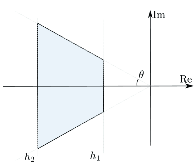
Figure 1: Desired LMI region in the complex plain.

The next to be analyzed is selection of the constants $h_{1}$, $h_{2}$ and $\theta$ for the LMI-based surface design.

5.1.1 Assignment of $h_{2}$:

In order to assign a proper boundary value $h_{2}$, one can consider an approximated first-order response of a linear system of the form $c_{h_{2}}(t)=1-\exp(t/T_{h_{2}})$. In order to obtain a time constant such that the first-order response to the step as $\lim_{t\rightarrow\infty}c_{h_{2}}(t)=\bar{y}_{2}$, the response should reach $63.2\%$ of the total desired amplitude. Then, from a straightforward geometrical reasoning, the associated time constant can be approximated by

$$T_{h_{2}}\approx\sqrt{(0.632y_{d})^{2}-(\bar{y_{2}})^{2}}\,.$$ (33)

and consequently $h_{2}=1/T_{h_{2}}$.

5.1.2 Assignment of $h_{1}$:

Consider the mechanical sub-system and assume that the pressure difference between the chambers is the given input. Then, in terms of the pressure to control the second-order dynamics

$$\frac{d}{dt}\begin{bmatrix}x_{1}\\ x_{2}\end{bmatrix}=\begin{bmatrix}0&1\\ 0&-\frac{\sigma}{m}\end{bmatrix}\begin{bmatrix}x_{1}\\ x_{2}\end{bmatrix}+\begin{bmatrix}0\\ \frac{1}{\tau m}\end{bmatrix}AP\,,$$ (34)

and assuming $AP=-k_{h}x_{1}-\sigma_{h}x_{2}$ with the feedback constants in a hypothetical closed-loop

$$\frac{d}{dt}\begin{bmatrix}x_{1}\\ x_{2}\end{bmatrix}=\begin{bmatrix}0&1\\ -\frac{k_{h}}{\tau m}&-\frac{\sigma\tau+\sigma_{h}}{\tau m}\end{bmatrix}\begin{bmatrix}x_{1}\\ x_{2}\end{bmatrix},$$ (35)

or its summarized compact form $\frac{d}{dt}\begin{bmatrix}x_{1}&x_{2}\end{bmatrix}^{T}=A_{h}\begin{bmatrix}x_{1}&x_{2}\end{bmatrix}^{T}$, one can compute the eigenvalues as

$$\lambda_{1,2}(A_{h})=-\frac{\sigma\tau+\sigma_{h}}{2\tau m}\pm\frac{1}{2\tau m}\sqrt[2]{\left(\tau\sigma+\sigma_{h}\right)^{2}-4k_{h}\tau m}\,.$$ (36)

The critically damped case is when $(\tau\sigma+\sigma_{h})^{2}-4k_{h}\tau m=0$, and both eigenvalues have the same real part. Then, the step response of the position as output has a form $x_{1}(t)=1-\exp^{-\omega_{n}t}(1+\omega_{n}t)$ where $\omega_{n}=\frac{\sigma\tau+\sigma_{h}}{2\tau m}$. At the same time, if one approximates the step response by a first-order behavior, one can compute the time constant as

$$T_{h_{1}}=\frac{2m\tau}{\sigma\tau+\sigma_{h}}\,,$$ (37)

which implies that for a desired $T_{h_{1}}$, one can determine

$$\sigma_{h}=\frac{2m\tau}{T_{h_{1}}}-\sigma\tau\,.$$ (38)

Then, for a desired behavior of the mechanical sub-system, being related to its time constant $T_{h_{1}}$, one obtains

$$h_{1}=-\frac{\sigma\tau+\sigma_{h}}{2\tau m}$$ (39)

5.1.3 Parameter $\theta$:

For many practical reasons, it is convenient to have only real negative eigenvalues such that the mechanical response does exhibit an oscillating response. This can be done if the parameter $\theta=0$, and therefore the cone-constrained LMI region collapses only into the real line. However, this can cause computational problems or the feasibility of the LMI’s may be compromise. Parameter $\theta$ is introduced such that it can be adjusted in order to find a solution to the LMI, by choosing it as small as possible.

5.1.4 Bound for $\psi(t,e)$:

Moreover, assume that the largest mechanical perturbation is due to nonlinear fiction term, cf. (7), and rewrite it as

$$\psi(t,x_{2})=\frac{\tanh(\vartheta x_{2})\left[F_{c}+(F_{s}-F_{c})\text{exp}\left(-|x_{2}|^{\phi}\chi^{-\phi}\right)\right]}{x_{2}}\,,$$ (40)

which has its maximum as $x_{2}$ tends to zero. Then, one can find the bound as

$$\Psi=\sup\lim_{x_{2}\rightarrow 0}\psi(t,x_{2})\,.$$ (41)

5.2 STA design

In order to compute the $L$ value, take the perturbation $\delta_{z}$ and calculate its bound as

$$|\delta_{z}| \leq|\bar{\delta}_{3}(t)|+\kappa|\dot{e}_{2}(t)|\,.$$ (42)

Assuming that the system will be in a compact set, there exists a constant positive value $\overline{\ddot{q}}$ such that $|\dot{e}_{2}|\leq\overline{\ddot{q}}$. This way, the value of $L$ can be determined by

$$L=L_{3}+\kappa\overline{\ddot{q}}$$ (43)

6 Comparison with other SMC strategies

For the sake of clearness in the comparison presented in this section, the approach proposed in this paper will be called IS-STA.

A qualitative comparison with respect to the approach in [22] will be performed, taking into account that both of the approaches are based on the STA algorithm. Additionally, for both methodologies the velocity measurement is not needed in order to apply the control law.

The approach of [22] consists in three main steps: first, a tracking reference model is designed, secondly, a variable gain Levant’s differentiator is implemented, and finally, a variable gain STA based control law is designed. The variable gains for the differentiator and STA are updated using a norm observer. The sliding surface designed depends on the output and its derivatives, which are estimated by the variable gain Levant’s differentiator. It is important to remark, that the parameters used [22] are tuned so that the tracking performance for both of the approaches are similar.

According to [22], the following reference model is proposed:

$$y_{m}=\frac{(25)^{2}}{(s+25)^{2}}r\,.$$ (44)

The chosen Input to Output state variable filters have the form:

$$w_{u}(s)=\frac{1}{(s+5)^{2}}u\,,\quad w_{y}(s)=\frac{1}{(s+5)^{2}}q\,.$$ (45)

The variable gain differentiator implemented is the following

$$\dot{\hat{e}}_{1} =-3L_{vgst}^{1/4}(t,\hat{x})\lceil\hat{e}_{1}-e_{1}\rfloor^{3/4}-2(\hat{e}_{1}-e_{1})+\hat{e}_{2}\,,$$ (46)

$$\dot{\hat{e}}_{2} =-2.5L_{vgst}^{1/3}(t,\hat{x})\lceil\hat{e}_{1}-e_{1}\rfloor^{2/3}-3(\hat{e}_{1}-e_{1})+\hat{e}_{3}\,,$$

$$\dot{\hat{e}}_{3} =-1.5L_{vgst}^{1/2}(t,\hat{x})\lceil\hat{e}_{1}-e_{1}\rfloor^{1/2}-2(\hat{e}_{1}-e_{1})+\hat{e}_{4}\,,$$

$$\dot{\hat{e}}_{4} =-1.1L_{vgst}(t,\hat{x})\lceil\hat{e}_{1}-e_{1}\rfloor^{0}-(\hat{e}_{1}-e_{1})\,.$$

where the gains comes from:

$$\dot{\hat{x}} =-0.8\hat{x}(t)+10+1.5\left\|\begin{bmatrix}w_{u}&w_{y}\end{bmatrix}^{T}\right\|\,,$$ (47)

$$L_{vgst}(t,\hat{x}) =1.2|\hat{x}|+2|u|+7\,.$$

The control strategy consists of the following sliding surface and controller

$$\hat{\sigma}(t) =\hat{e}_{3}+2(25)\hat{e}_{2}+(25)^{2}e_{1}$$ (48)

$$u_{vgsta} =-\tilde{k}_{1}(t,\hat{x})\phi_{1}(\hat{\sigma})-\int_{0}^{t}\tilde{k}_{2}(\tau,\hat{x})\phi_{2}(\hat{x})d\tau\,,$$

$$\phi_{1}(\hat{\sigma}) =\lceil\hat{\sigma}\rfloor^{1/2}+\hat{\sigma}\,,$$

$$\phi_{2}(\hat{\sigma}) =\frac{1}{2}\lceil\hat{\sigma}\rfloor^{0}+\frac{3}{2}\lceil\hat{\sigma}\rfloor^{1/2}+\hat{\sigma}\,,$$

where the gains $\tilde{k}_{1}(t,\hat{x})$ and $\tilde{k}_{2}(t,\hat{x})$ are designed according to [22], taking into account the following bounds of the perturbations $\rho_{1}=0$ and $\rho_{2}=10|\hat{e}_{2}|+5|e_{1}|+\hat{x}+1$ and the constants $\delta_{k}=0.01$, $\varepsilon_{k}=1\times 10^{-3}$, resulting in:

$$\tilde{k}_{1} =\delta_{k}+\frac{1}{4\varepsilon_{k}}\rho_{2}^{2}+2\varepsilon_{k}\rho_{2}+\varepsilon_{k}+2\varepsilon_{k}\left(1+4\varepsilon_{k}^{2}\right)\,,$$

$$\tilde{k}_{2} =1+4\varepsilon_{k}^{2}+2\varepsilon_{k}\tilde{k}_{1}\,.$$

The simulations were performed using a band limited white noise in the measurements, similar to the one presented in the real plant sensors, with noise power of $1\times 10^{-9}$ and a sample time of $5\times 10^{-6}$. The details about the designed trajectories are presented in the experimental evaluation.

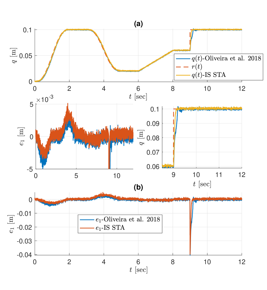
Figure 2: Comparison of the position $q$ and tracking error $e_{1}$. $r(t)$ corresponds to the reference to be tracked, $q(t)$- IS STA is the proposed approach and $q(t)$- Oliveira et al. 2018 is the approach presented in [22].

It can be observed in Figure 2, that the tracking is well performed by the two methodologies. In Figure 2-(b) the errors are presented. Although the IS STA appears to be better in the first $3$ seconds, the approach of [22] works similarly well in second stage of the trajectory, from $t=3$ to $t=5$. During the transient of the step response, the IS STA slightly outperforms [22].

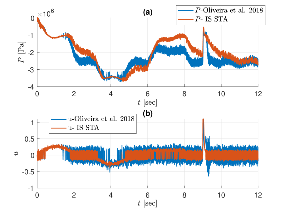
Figure 3: Comparison of the pressure variable $P$ and control signal $u$ corresponds to the reference to be tracked, IS STA is the proposed approach and Oliveira et al. 2018 is the approach presented in [22].

In Figure 3 the pressure diference $P$ and the control signal $u(t)$ are presented. From the control signal $u(t)$ it is clear that $u$-IS STA is smaller in amplitude than the one from the $u$-Oliveira et al. 2018. This can be caused by the noise in the measurement which is propagated not only in the Variable Gain Super-Twisting, but also via the third order differentiator. One may decrease gains in order to reduce the effect of the noise in the control input. However, this also make the performance to decrease.

7 Experimental Evaluation

7.1 Experimental setup

In this section, the experimental validation of the proposed control approach is provided. The presented control solution is implemented in the laboratory test bench [24], see laboratory view shown in Fig. 4. The hydraulic setup is composed by a one-side-rod cylinder with a moving load carrier, mounted in a linear slide bearing, and one translational degree of freedom $q$.

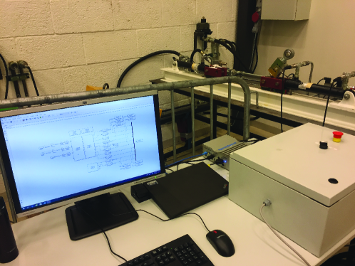
Figure 4: Experimental test bench of hydraulic actuator (laboratory view).

The cylinder is connected via a 4 ways / 3 positions servo-valve with an internal closed-loop spool control, connected to the hydraulic power unit, cf. schematic diagram of the hydraulic circuit shown if Fig. 5.

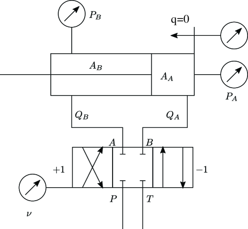
Figure 5: Schematic diagram of the hydraulic circuit of the actuator system.

The supply parameters are set to $10$ MPa pressure and $40$ liter/min volumetric flow. More details on the hardware components can be found in [24]. Since the low-level controlled servo-valve receives the input reference signal in percentage of the orifice opening, the control signal $u$ and correspondingly $g$ (cf. with section 6.3) is inherently unitless i.e. $u\in[-1,+1]$. Worth noting is also that the control algorithms are implemented in Simulink®Real-Time on a Speedgoat™platform with 2 kHz sampling rate.

7.2 Motion trajectories

The trajectories were designed as piece-wise continuous functions for different time instants. From the time $t=0$ to $t=2$, a quintic smooth polynomial trajectory is tracked, starting from $q(0)=0$ m to $q(2)=0.1$ m in a fashion of smooth robotic trajectories, cf. [30]. Then, the value is maintained until $t=3$ s and then switched to another quintic polynomial trajectory from $q(3)=0.1$ m to $q(5)=0.02$ m. Then a ramp is assumed from $t=6$ s to $t=8$ s and, finally, a step from $q(9)=0.1$ m is imposed. Worth noting is that although the final step is not a smooth trajectory, as required for $r(t)$, the proposed control approach is able to track it as well.

7.3 Implemented control scheme

The first implementation issue of the applied control scheme is the dead-zone effect in the servo-valve opening orifice. This effect, as shown in [24], is (nearly) static around the $10\,\%$ of the opening range. Therefore, the dead-zone is compensated in feed-forwarding via an inverse map of the form:

$$\tilde{u}=\frac{1}{2}D_{s}\text{sign}(u)+u$$ (49)

where $D_{s}>0$ is the dead-zone size.

Second, in the control related modeling and analysis, the servo valve dynamics was not taken into account. Such actuator dynamics can be pre-compensated in the same way as dead-zone effect. From the previous work [24], the parameters of the servo-valve input-output behavior of the form (1) are obtained. Then, a low-pass filter is implemented in order to count for the fast (but still not zero) dynamics of the servo valve. The overall control value has then the form

$$g=\frac{1}{\left(\mu_{c}\varphi+1\right)^{2}}\left[\frac{1}{2}D_{s}\text{sign}(u)+u\right]$$ (50)

where $\varphi$ is the Laplace variable and $\mu_{c}>0$ is a design parameter chosen to be equal to the servo-valve actuator time constant. The identified parameters are given in [24]. Moreover, we stress that due to the dead-zone compensation the chattering effect may be increased in the control zero crossing. In that sense, the set low-pass filter complies along with the servo-valve bandwidth, reducing the chattering of the effective control value $g(t)$. The overall control strategy implemented is presented in Figure 6.

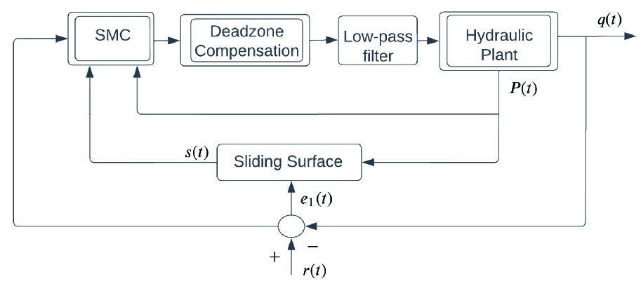
Figure 6: Schematic of the overall control strategy implemented.

7.4 Auxiliary frequency domain analyze

Based on the experimental evaluations, the authors notice some practical issues that are worth to be addressed as below. The stability of the sliding dynamics can also be lost by changing the design parameters $h_{1}$ and $h_{2}$. In this section, based on the concept of phase deficit [4], a possible explanation to this phenomena is given. In a nutshell, the phase deficit represents a certain measure of robustness for a finite-time controller, similar to concept of the phase margin usable for asymptotic linear controllers. It can be seen as the angular difference of the reciprocal of negative inverse Describing Function (DF) of a nonlinear control law and the plant’s Nyquist plot [4].

Let us analyze the output of the system that is assumed to have the form: $y(t)=a_{y}\sin(\Omega t+\phi_{y})$, where $\Omega$ is the frequency and $a_{y}$ is the amplitude of steady oscillations, and $\phi_{y}$ is the phase lag. Assuming that the dynamic sliding surface is a periodic input $s(t)=a_{s}\sin(\omega t)$ being $a_{s}>0$ the amplitude of the oscillations in the surface $s$, it is possible to find the oscillatory reaction $y(t)$, and more important, an explanation on how it is affected by the design of the variable $h_{2}$. Consider that the transfer function function of the closed loop has the form

$$G_{f}(\varphi)=\frac{1}{\frac{1}{T_{s}}\varphi+N_{f}(a_{y})}\,$$ (51)

where the positive constant $T_{s}$ is a time constant dependent on the design parameters $h_{1}$ and $h_{2}$, and $N_{f}$ is the DF of the STA

$$N_{f}(a_{y})=\frac{2k_{1}L\gamma(1.25)}{\sqrt{\pi}\gamma(1.75)}a_{y}^{-1/2}=\gamma_{a}a_{y}^{-1/2}\,,$$ (52)

where $\gamma(\cdot)$ is the gamma-function, as it is presented in [3]. Setting $a_{1}=\frac{4k_{2}L^{2}}{\pi\omega}$ and following [3], one can compute the amplitude of the propagated oscillations as: $a_{y}=a_{1}|G_{f}(jw)|$, or equivalently:

$$\frac{w^{2}}{T_{s}^{2}}a_{y}^{2}+\gamma^{2}a_{y}-a_{1}^{2}=0\,,$$ (53)

whose solution is given by

$$a_{y}=\frac{T_{s}^{2}}{2w^{2}}\left(-\gamma^{2}+\sqrt{\gamma^{4}+4T_{s}^{2}\omega^{2}a_{1}^{2}}\right)\,.$$ (54)

Computing its phase deficit it yields [3] :

$$\phi_{d}=\frac{\pi}{2}-\arctan\left(\frac{1}{\sqrt{2}}\sqrt{-1+\sqrt{1+\frac{64k_{2}^{2}\rho^{2}}{T_{s}^{4}\pi^{2}\gamma^{4}}}}\right)\,,$$ (55)

ensuring that the phase deficit approaches to zero as $T_{s}$ tends to zero as well. This gives us an explanation why the nominal system’s response can not be made arbitrarily fast without compromising the system’s stability, and implies the selection of $h_{2}$ margin should be additionally restricted, cf. with section 5.1.1.

7.5 Experimental results

For the control evaluation, the computed parameters for the LMI conditions are $h_{2}=-5$ and $h_{1}=-1$, these from the assigned time constants $T_{h_{2}}=1/5$ s and $T_{h_{1}}=1$ s. The parameter $\theta$ is left to be small enough such that the LMI is still feasible but, at the same time, tries to restrict the imaginary part of the resulting poles. In this work, $\theta=\pi/20$ was chosen. From the aforementioned analysis one can get $\Psi=0.5$. Finally, for the STA, we assume the gains which minimize the amplitude of chattering as $k_{1}=1.1$ and $k_{2}=2.028$, see [26], so that the scaling condition becomes $\rho>2(1.6303)L$. The computed boundary constant is $L=1.347$, and the assigned scaling factor is $\rho=10$. A summary of the parameters used for this experimental results is presented in table 1 with the corresponding methodology section.

Table 1: Summary of the parameters and its corresponding section.

Parameter:	Value:	Design section:
$h_{1}$	1110.1	Section 5.1.2
$h_{2}$	10.1	Section 5.1.1
$\theta$	23.113231	Section 5.1.3
$k_{1}$	1.1	c.f. [26]
$k_{2}$	2.028
$\rho$	10	Section 5.1.4

The designed motion trajectory is evaluated experimentally, as shown by the dotted line in Fig. 7 (a). It can be seen that the cylinder position $q(t)$ follows the desired trajectory, being uniformly close to the reference value $r(t)$. The measured piston position is shown by blue solid line and the reference is shown by the dotted black line in Fig. 7 (a). It can be recognized that the position is tracked accurately even in the case of a discontinuous (step) change at $t=9\,\,\text{s}$. The corresponding tracking error is also shown in Fig. 9 (b). Although the velocity is not available and, thus, not used in the proposed control approach, it is estimated using robust exact differentiator toolbox [2] for the sake of a better visualization of the controlled motion. Figure 7 (b) discloses that the estimated velocity is well in line with derivative of the reference value.

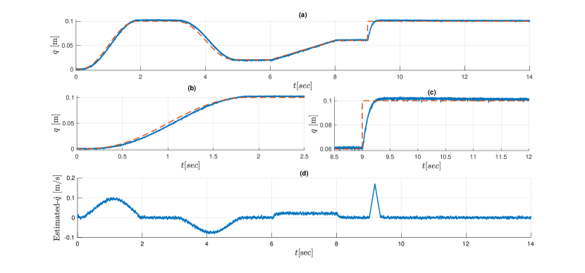
Figure 7: Measured position (versus reference) in (a), zoom from $t=0$ to $t=2.5$ seconds is presented in (b), zoom on the tracking position from $t=8.5$ to $t=12$ seconds is presented in (c) and the estimated velocity of the controlled motion trajectory is shown in (d).

Figure 8 shows the differential pressure, i.e. measured pressure difference between the right and left chambers, in (a) and the resulted control signal which is applied to the servo-valve in (b). Worth recognizing is that the control signal is continuous. Some chattering pattern, where the control signal appears to oscillate between $\pm\,0.1$, appears at several phases of steady-state and corresponds to the dead-zone effect in the servo-valve. Recall that the latter is pre-compensated in feed-forward by the dead-zone inverse. Also note that the servo-valve blocks energizing the hydraulic circuits within the dead-zone, so that a low-amplitude chattering is slightly outside of $\pm\,0.1$. Since the second-order actuator dynamics provides the corresponding low-pass filtering, such dead-zone related chattering is irrelevant for loading of the hydraulic circuits. From Fig. 8 (a), the pressure is acting as virtual control for the sub-mechanical system. It is important to recall that the $P$ variable is the differential pressure so that its negative values have reasoning for the selected motion direction. Also worth recalling that within dead-zone, the valve is locking the hydraulic circuit from one side and, consequently, one of the chambers remains pressurized. This is explaining the non-zero $P(t)$ values where there is no apparent motion of the cylinder piston, cf. Fig. 7 and Fig. 8 (a). The load pressure magnitude remain below $40\,\,\text{bar}$ while the supply pressure is $100\,\,\text{bar}$. Figure 8 (b) discloses also the continuous control signal (apart from the dead-zone chattering) and that the control signal is never saturated.

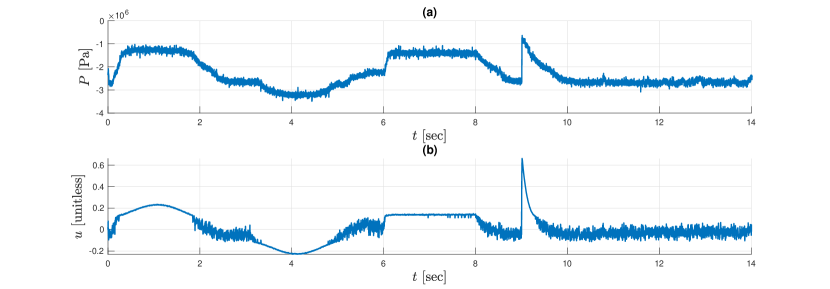
Figure 8: Measure differential pressure (as virtual control) in (a) and the control signal in (b).

In Fig. 9, zoom-in plot of the output tracking error and the sliding variable are shown in (a) and (b), respectively. Important to notice is that the sliding mode may be temporary lost when the assumed conditions about perturbations, cf. (11) and (13), are violated, like in case of the applied step reference at $t=9$ s. Even then, the sliding mode is subsequently recovered and the tracking is well performed.

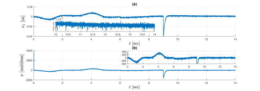
Figure 9: Measured output tracking error in (a) and the sliding mode variable in (b).

It is important to mention that the convergence velocity may be increased by the scaling factor $\rho$. In Figure 10 the step response with respect to different values of $\rho$ is presented. However, the bigger the gain $\rho$, the bigger the control input. Another important issue with increasing the gain is the amplitude of the chattering effect. Increasing the gain may considerable increase the chattering produced by the noise.

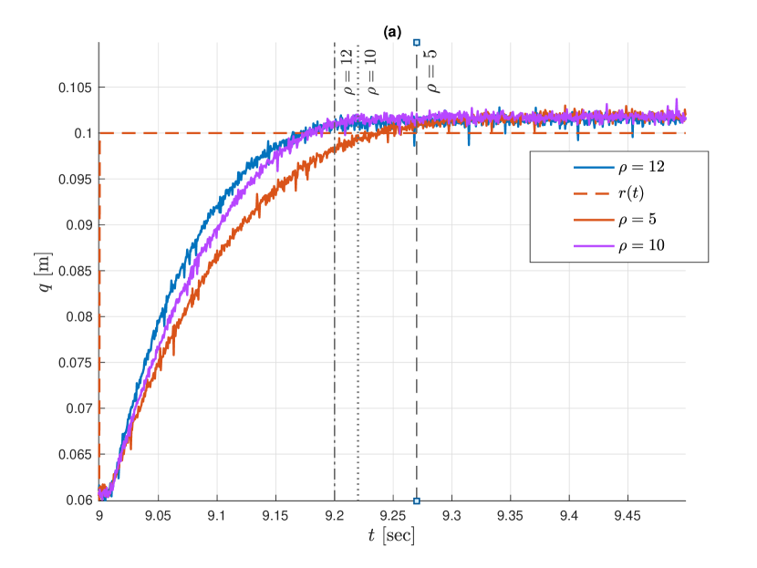
Figure 10: Comparison of the step response with different values of $\rho$.

A brief video of the presented experimental results is available under https://youtu.be/_dnwD7Ens-k.

7.6 Quantitative measures of performance

In this section, some quantitative measures of the experimental results are given. Let us define the following performance indices:

1. Maximal absolute value of the tracking error

   $$M_{e}=\max_{i=1,2,\ldots,N}\left\{|e_{1}(i)|\right\}\,,$$ (56)

   being $N$ the number of obtained values recorded.

2. Average tracking error

   $$\mu_{e}=\frac{1}{N}\sum_{i=1}^{N}|e_{1}(i)|\,.$$ (57)

3. Standard deviation performance index

   $$\sigma_{e}=\sqrt{\frac{1}{N}\sum_{i=1}^{N}\left(|e_{1}(i)|-\mu_{e}\right)^{2}}\,.$$ (58)

The maximal absolute value of the tracking error can be considered as an index of the tracking accuracy. Meanwhile, the average tracking error and the standard deviation performance show the average tracking performance and the deviation of the tracking errors, respectively. Finally, the Integral Square Error (ISE) will be taken into account.

The experimentally obtained values for every index are presented in table 2, taking the error in the last step response, that is, from $t=10$ to $t=14$.

Table 2: Values of perfomance indices

Index:	Value:
$M_{e}$	0.0064
$\mu_{e}$	0.0011
$\sigma_{e}$	3.4598 $\times 10^{-6}$
ISE	$333.7830$
Percentage of steady state error	$0.55\%$

The percentage of the steady state error is obtained taking the average tracking error as a percentage of the total cylinder drive, that is $0.20$ m.

8 Conclusion

A new practical control approach, based on the sliding mode STA, is introduced and applied to a hydraulic cylinder actuator. The proposed method is proved to track a smooth trajectory in presence of both matched and unmatched perturbations, producing an acceptably small and ultimately bounded tracking error. Important to notice is that via the designed integral sliding surface, the velocity state is fully excluded and needs to be neither measured nor estimated for implementing the proposed controller. The design methodology for such surface is developed in terms of an LMI. The feasibility of the proposed approach is shown via experimental results achieved on a standard industrial hydraulic actuator in laboratory setting, without additional measurements and extensive modeling and identification.

Leonid Fridman and Manuel A. Estrada are grateful for the financial support of CONACyT (Consejo Nacional de Ciencia y Tecnología): CVU 833748; PAPIIT-UNAM (Programa de Apoyo a Proyectos de Investigación e Innovación Tecnológica): Project IN106622.

Appendix A Proof of Theorem 1

Assume the following Lyapunov function candidate $V(e)=e^{T}Me$. Its derivative along the trajectories of $\dot{e}=(A_{n}-BR)e+\psi(t,e)He$ has the form

$$\dot{V}(e) =e^{T}(t)\left[MA_{n}+A_{n}^{T}M+\psi(t,e)\left(H^{T}M+MH\right)\right]e(t)$$ (59)

$$-e(t)^{T}\left(K^{T}B^{T}M+MBK\right)e(t)$$

$$\leq e^{T}(t)\left[MA_{n}+A_{n}^{T}M-K^{T}B^{T}M-MBK\right.$$

$$\left.+\Psi\left(H^{T}M+MH\right)\right]e(t)$$

Then, as shown in [8], the system is quadratically stable if there exists such $R\in\mathbb{R}^{3}$ and $M=M^{T}>0$ that (20) is satisfied. The necessity comes from the quadratic stabilizability. If the system is not quadratically stabilizable, then there is no solution of (20). This concludes the proof.

Appendix B Proof of Lemma 3

If $\beta(t)\neq 0$, the closed loop of mechanical sub-system with the virtual control has the form $\dot{e}(t)=(A_{n}-BK)e+\psi(t,x)He+\beta(t)D$, where $D^{T}=\begin{bmatrix}0&1&0\end{bmatrix}$. Taking the Lyapunov function candidate $V=e^{T}Me$, its derivative is

$$\dot{V}(e) =e^{T}(t)\left[MA_{n}+A_{n}^{T}M+\psi(t,e)\left(H^{T}M+MH\right)\right]e(t)$$

$$-e(t)^{T}\left(K^{T}B^{T}M+MBK\right)e(t)$$

$$+\beta(t)\left(D^{T}Me+e^{T}MD\right)$$

$$\leq e^{T}(t)\left[MA_{n}+A_{n}^{T}M-K^{T}B^{T}M-MBK\right.$$

$$\left.+\Psi\left(H^{T}M+MH\right)\right]e(t)+2\lambda_{max}(M)\beta_{M}\|e(t)\|\,.$$

If the LMI (20) is satisfied, then there exists $\mu(M)>0$ such that

$$\dot{V}(e)\leq-\mu(M)\|e(t)\|^{2}+2\lambda_{max}(M)\beta_{M}\|e(t)\|$$ (60)

Assuming a constant $0<\theta_{V}<1$, the following is satisfied

$$\dot{V}(e)\leq-(1-\theta_{V})\mu(M)\|e(t)\|^{2}\,,\,\|e(t)\|\geq\frac{2\lambda_{max}(M)\beta_{M}}{\theta_{V}\mu(M)}\,.$$

By Theorem 4.18 from [12], the system’s trajectories are then ultimately uniformly bounded and the bound (21) is satisfied.

Appendix C Proof of Lemma 4

In order to show the reachability of the sliding surface (22), consider the following control

$$u(t)= -\frac{V_{t}}{4\tau EC_{q}}K_{s}\text{sign}(s)$$ (61)

$$+\frac{V_{t}}{4\tau EC_{q}}\left[\gamma_{1}e_{1}-\left(\gamma_{2}+\frac{4EC_{qp}}{V_{t}}\right)\eta\right]$$

for a positive constant $K_{s}$. Therefore, the reachability condition has the form:

$$s\dot{s} =s\left[-K_{s}\text{sign}(s)+\bar{\delta}_{3}(t)+\kappa e_{2}\right]$$ (62)

$$\leq-K_{s}|s|+|s||\bar{\delta}_{3}(t)|+|s|\kappa|e_{2}|$$

$$\leq-|s|\left(K_{s}+L_{3}+\kappa|e_{2}|\right)\,,$$

since $|e_{2}|\leq C_{e_{2}}$, there always exist $K_{s}>L_{3}+\kappa C_{e_{2}}$, such that with $\bar{K}_{s}=K_{s}-L_{2}-\kappa C_{e_{2}}$, and the following is satisfied:

$$s\dot{s}\leq-\bar{K}_{s}|s|<0\,,$$ (63)

proving that there always exist a control law (indepedent of the uncertainties and perturbations) that ensures the trajectories converges to the manifold $s(t)\equiv 0$, and therefore, they remain in such manifold.

Appendix D Proof of Lemma 6

To prove the stability of $s=0$ and $z=0$, consider the following change of coordinates introduced in [20]: $\zeta^{T}=\begin{bmatrix}\zeta_{1}&\zeta_{2}\end{bmatrix}=\begin{bmatrix}\lceil s\rfloor^{1/2}&z\end{bmatrix}$. Computing its dynamics yields

$$\dot{\zeta}=\frac{\partial\zeta_{1}}{\partial s}\begin{bmatrix}-k_{1}\rho&1\\ -k_{2}\rho^{2}&0\end{bmatrix}\zeta+\begin{bmatrix}0\\ \delta_{z}(t,e)\end{bmatrix}=\frac{\partial\zeta_{1}}{\partial s}A_{s}\zeta+G\delta_{z}(t,e)\,,$$ (64)

where $G^{T}=\begin{bmatrix}0&1\end{bmatrix}$. Note that this term is always positive and bounded from below as $\left|\frac{\partial\zeta_{1}}{\partial s}\right|\geq 1$. Consider the following scaling of the states

$$\xi=\begin{bmatrix}\xi_{1}\\ \xi_{2}\end{bmatrix}=\Gamma^{-1}\zeta\quad\text{with}\quad\Gamma=\begin{bmatrix}\rho&0\\ 0&\rho^{2}\end{bmatrix}\,,$$ (65)

so that the dynamics has the form $\dot{\xi}=\frac{\partial\xi_{1}}{\partial s}\Gamma^{-1}M_{s}\xi+\Gamma^{-1}G\delta_{z}(t,e)$ . Then one has

$$\frac{d\xi}{dt}=\frac{\partial\xi_{1}}{\partial s}\left(\rho A_{k}\xi+G\frac{\delta_{z}(t,e)}{\frac{\partial\xi_{1}}{\partial s}\rho}\right)\,.$$ (66)

Consider the Lyapunov function candidate $V_{s}=\xi^{T}M_{k}\xi$, whose derivatives along the trajectories of the $\dot{\xi}$ vector field has the form

$$\frac{dV_{s}(t)}{dt} =\dot{\xi}^{T}M_{k}\xi+\xi^{T}M_{k}\dot{\xi}$$ (67)

$$= \rho\frac{\partial\xi_{1}}{\partial s}\xi^{T}\left(A_{k}^{T}M_{k}+M_{k}A_{k}\right)+2\frac{\partial\xi_{1}}{\partial s}\xi^{T}M_{k}G\frac{\delta_{z}(t,e)}{\frac{\partial\xi_{1}}{\partial s}\rho}\,.$$

Note that for any Hurwitz matrix $A_{k}$, there exists always a solution $M_{k}$ of $A_{k}^{T}M_{k}+M_{k}A_{k}=-\mathbb{I}$, so that

$$\frac{dV_{s}(t)}{dt}=-\frac{\partial\xi_{1}}{\partial s}\left(\rho\xi^{T}\xi-2\xi^{T}M_{k}G\frac{\delta_{z}(t,e)}{\frac{\partial\xi_{1}}{\partial s}\rho}\right)\,.$$ (68)

For the assumed $|\delta_{z}|\leq L|\xi_{1}|$, one can obtain the following bound

$$\frac{dV_{s}(t)}{dt}\leq-\frac{\partial\xi_{1}}{\partial s}\left(\rho-2L\lambda_{max}(M_{k})\right)\|\xi\|^{2}\,.$$ (69)

It is sufficient that only the gain $\rho$ satisfies (29). Then, the stability of the surface’s origin and control law of the closed loop are ensured for a sufficiently large value of $\rho$.

References

- [1] Andrew Alleyne and Rui Liu. A simplified approach to force control for electro-hydraulic systems. Control Engineering Practice, 8(12):1347–1356, 2000.
- [2] Benedikt Andritsch, Martin Horn, Stefan Koch, Helmut Niederwieser, Maximilian Wetzlinger, and Markus Reichhartinger. The robust exact differentiator toolbox revisited: Filtering and discretization features. In 2021 IEEE International Conference on Mechatronics (ICM), pages 01–06. IEEE, 2021.
- [3] Igor Boiko. On phase deficit of the super-twisting second-order sliding mode control algorithm. International Journal of Robust and Nonlinear Control, 30(16):6351–6362, 2020.
- [4] Igor M Boiko. On frequency-domain criterion of finite-time convergence of second-order sliding mode control algorithms. Automatica, 47(9):1969–1973, 2011.
- [5] Adrian Bonchis, Peter I Corke, David C Rye, and Quang Phuc Ha. Variable structure methods in hydraulic servo systems control. Automatica, 37(4):589–595, 2001.
- [6] Riccardo Checchin, Michael Ruderman, and Roberto Oboe. Robust two-degrees-of-freedom control of hydraulic drive with remote wireless operation. In 2023 IEEE International Conference on Mechatronics (ICM), pages 1–6, 2023.
- [7] Han Ho Choi. LMI-based sliding surface design for integral sliding mode control of mismatched uncertain systems. IEEE Transactions on Automatic Control, 52(4):736–742, 2007.
- [8] Martin Corless. Robust stability analysis and controller design with quadratic Lyapunov functions, pages 181–203. Springer, Berlin, Heidelberg, 1994.
- [9] C. Edwards, A. Akoachere, and S.K. Spurgeon. Sliding-mode output feedback controller design using linear matrix inequalities. IEEE Transactions on Automatic Control, 46(1):115–119, 2001.
- [10] Christopher Edwards and Sarah Spurgeon. Sliding mode control: theory and applications. CRC Press, 1998.
- [11] AF Filippov. Differential Equations with Discontinuous Right-hand Sides. Dordrecht: Kluwer Academic Publishers, 1988.
- [12] Hassan K. Khalil. Nonlinear Systems. Prentice Hall, New Jersey, 2001.
- [13] Stefan Koch and Markus Reichhartinger. Observer-based sliding mode control of hydraulic cylinders in the presence of unknown load forces. E & I Elektrotechnik und Informationstechnik, 133(6):253–260, 2016.
- [14] Jan Komsta, Nils van Oijen, and Peter Antoszkiewicz. Integral sliding mode compensator for load pressure control of die-cushion cylinder drive. Control Engineering Practice, 21(5):708–718, 2013.
- [15] Arie Levant. Sliding order and sliding accuracy in sliding mode control. International Journal of Control, 58(6):1247–1263, 1993.
- [16] G.P. Liu and S. Daley. Optimal-tuning nonlinear PID control of hydraulic systems. Control Engineering Practice, 8(9):1045–1053, 2000.
- [17] Alexander G Loukianov, Jorge Rivera, Yuri V Orlov, and Edgar Yoshio Morales Teraoka. Robust trajectory tracking for an electrohydraulic actuator. IEEE Transactions on Industrial Electronics, 56(9):3523–3531, 2008.
- [18] Jouni Mattila, Janne Koivumäki, Darwin G Caldwell, and Claudio Semini. A survey on control of hydraulic robotic manipulators with projection to future trends. IEEE/ASME Transactions on Mechatronics, 22(2):669–680, 2017.
- [19] Herbert E Merritt. Hydraulic control systems. John Wiley and Sons, 1967.
- [20] Jaime A. Moreno. Lyapunov Approach for Analysis and Design of Second Order Sliding Mode Algorithms, pages 113–149. Springer, Berlin, Heidelberg, 2012.
- [21] Navid Niksefat and Nariman Sepehri. Designing robust force control of hydraulic actuators despite system and environmental uncertainties. IEEE Control Systems Magazine, 21(2):66–77, 2001.
- [22] Tiago Roux Oliveira, Victor Hugo Pereira Rodrigues, Antonio Estrada, and Leonid Fridman. Output-feedback variable gain super-twisting algorithm for arbitrary relative degree systems. International Journal of Control, 91(9):2043–2059, 2018.
- [23] Daniel Ortiz Morales, Simon Westerberg, Pedro X La Hera, Uwe Mettin, Leonid Freidovich, and Anton S Shiriaev. Increasing the level of automation in the forestry logging process with crane trajectory planning and control. Journal of Field Robotics, 31(3):343–363, 2014.
- [24] Philipp Pasolli and Michael Ruderman. Linearized piecewise affine in control and states hydraulic system: Modeling and identification. In IEEE 44th Annual Conference of the Industrial Electronics Society (IECON), pages 4537–4544, 2018.
- [25] Henrik C Pedersen and Torben O Andersen. Pressure feedback in fluid power systems—active damping explained and exemplified. IEEE Transactions on Control Systems Technology, 26(1):102–113, 2017.
- [26] Ulises Pérez-Ventura and Leonid Fridman. Design of super-twisting control gains: A describing function based methodology. Automatica, 99:175–180, 2019.
- [27] Michael Ruderman. Full- and reduced-order model of hydraulic cylinder for motion control. IEEE 43rd Annual Conference of the Industrial Electronics Society (IECON), pages 7275–7280, 2017.
- [28] Michael Ruderman, Leonid Fridman, and Philipp Pasolli. Virtual sensing of load forces in hydraulic actuators using second-and higher-order sliding modes. Control Engineering Practice, 92:104151, 2019.
- [29] Richard Seeber and Martin Horn. Stability proof for a well-established super-twisting parameter setting. Automatica, 84:241–243, 2017.
- [30] Mark W Spong, Seth Hutchinson, Mathukumalli Vidyasagar, et al. Robot modeling and control, volume 3. Wiley New York, 2006.
- [31] Vadim I Utkin. Sliding modes in control and optimization. Springer Science & Business Media, 1992.
- [32] Bin Yao, Fanping Bu, J. Reedy, and G.T.-C. Chiu. Adaptive robust motion control of single-rod hydraulic actuators: theory and experiments. IEEE/ASME Transactions on Mechatronics, 5(1):79–91, 2000.