Accelerated gradient descent: A guaranteed bound
for a heuristic restart strategy

Abstract

The $\mathcal{O}(1/k^{2})$ convergence rate in function value of accelerated gradient descent is optimal, but there are many modifications that have been used to speed up convergence in practice. Among these modifications are restarts, that is, starting the algorithm with the current iteration being considered as the initial point. We focus on the adaptive restart techniques introduced by O’Donoghue and Candès, specifically their gradient restart strategy. While the gradient restart strategy is a heuristic in general, we prove that applying gradient restarts preserves and in fact improves the $\mathcal{O}(1/k^{2})$ bound, hence establishing function value convergence, for one-dimensional functions. Applications of our results to separable and nearly separable functions are presented.

2010 Mathematics Subject Classification: Primary 90C25, 65K05; Secondary 65K10, 49M27.

1 Introduction

In 1983, Nesterov introduced acceleration to the classical gradient descent method [Nesterov(1983)]. This acceleration method involves the addition of an extrapolation based on previous iterates, the new iterate is then computed as a classical gradient step from this extrapolation. Accelerated gradient descent (AGD) is also known as gradient descent with momentum. This is because the extrapolation step is computed using an increasing sequence of scalars. Due to this added momentum AGD is a non-monotonic method as extrapolated points can overshoot the minimizer and cause an increase in function value.

Several restarting algorithms have been proposed recently as discussed in Section 2.1. Restarting means that the momentum term is set to its initial value of zero, and the current iteration is used as the new starting point. In effect, this deletes the memory used previously to compute the extrapolation steps.

O’Donoghue and Candès introduced an adaptive restart strategy that does not depend on any properties of the objective function [O’Donoghue and Candès(2015)]. The authors offer two heuristic schemes to restart AGD. The first is a function value scheme that restarts whenever non-monotonicity is detected, and the second restarts when the gradient makes an obtuse angle with the direction of the iterates. The latter scheme uses only already computed information. The authors suggest that the gradient based scheme is favorable as it is more numerically stable. While both schemes perform well in practice and tend to drastically improve the performance of AGD, unlike AGD, there is no proof of function value convergence for the restarted scheme. The authors have provided an analysis when the objective is quadratic and suggest that this analysis carries over to a quadratic region around the minimizer. There have however been examples, such as in the work by Hinder and Lubin [Hinder and Lubin(2020)] who give a simple function for which the restarts drastically underperform until the iterates get close to the minimizer [Hinder and Lubin(2020)]. Recall that a function $f:\R^{n}\rightarrow\R$ is L-smooth if it has Lipschitz continuous gradient, i.e., for all $x$ and $y$ in $\R^{n}$ we have,

$$\norm{\gf{x}-\gf{y}}\leq L\norm{x-y}.$$ (1)

Throughout the remainder of this paper, we assume that

$$f:\R^{n}\rightarrow\R L L>0 S:=\operatorname*{Argmin}f\neq\varnothing$$ is convex and -smooth, where , and (2)

and we set

$$f^{*}:=\min f(\R^{n})$$. (3)

In this paper we provide analysis for the case $n=1$. Our results, primarily Theorem 3.8 and Theorem 3.10 below, reveal that applying the gradient restart improves the classical right-hand side bound of AGD and hence preserves the function value convergence of the iterates of the restarted scheme. Unlike the O’Donoghue and Candès restart scheme, our analysis varies in that if the restart condition (see 16 below) is satisfied then we restart at $x_{k+1}$ rather than $x_{k}$. Computational experiments (see Appendix D and Appendix E) suggest that in practice restarting from $x_{k+1}$ offers slightly better practical performance for $n\geq 1$.

2 Framework and Related Works

Recalling 2, our framework for AGD is that of an unconstrained convex optimization problem

$$\min_{x\in\R^{n}}f(x).$$ (4)

Let $(t_{k})_{{k\in{\mathbb{N}}}}$ be a sequence of scalars such that $t_{0}=1$ and $(\forall k\geq 1)$ (see, e.g., [Beck and Teboulle(2009)])

$$t_{k}\geq\tfrac{k+2}{2}\geq 1=t_{0}\;\text{and}\;t_{k}^{2}\geq t^{2}_{k+1}-t_{k+1}.$$ (5)

Two popular choices for the sequence of $t_{k}$ are given by,

$$t_{k+1}=\tfrac{1+\sqrt{1+4t_{k}^{2}}}{2},\;\;\;t_{k}=\tfrac{k+2}{2}.$$ (6)

Let $x_{0}\in\R^{n}$, and set $y_{0}=x_{0}$. Throughout this paper we set

$$T={\operatorname{Id}-\tfrac{1}{L}\nabla f}.$$ (7)

Classical AGD updates $x_{0}$ $(\forall k\in\mathbb{N})$ as follows:

$$x_{k+1} :=T(y_{k})$$ (8a)

$$y_{k+1} :=x_{k+1}+\tfrac{t_{k}-1}{t_{k+1}}\left(x_{k+1}-x_{k}\right).$$ (8b)

We set

$$x^{*}:=P_{S}(x_{0})\in S,$$ (9)

where $P_{S}$ denotes the orthogonal projection (this is also known as the closest point mapping) onto the set $S$ which is convex, closed, and by assumption (see 2) nonempty.

Note that the classical upper bound for AGD is $(\forall{k\in{\mathbb{N}}})$

$$f(x_{k})-f^{*}\leq\frac{2L\norm{x_{0}-x^{*}}^{2}}{(k+1)^{2}}.$$ (10)

We now recall the following useful fact which will be used later.

Fact 1.

(see [Beck(2017), Theorem 10.16]) Let $x\in\R^{n}$ and let $y\in\R^{n}$. Then

$$f(x)-f(T(y))\geq\tfrac{L}{2}\norm{x-T(y)}^{2}-\tfrac{L}{2}\norm{x-y}^{2}.$$ (11)

2.1 Restarts

We will focus on adaptive restart strategies. These strategies restart the algorithm according to whether some condition is satisfied at the current iteration. In [O’Donoghue and Candès(2015)] O’Donoghue and Candès proposed two conditions for restarts: the function value and gradient based conditions. The function value condition imposes restarts whenever

$$f(x_{k+1})>f(x_{k}).$$ (12)

On the other hand, the gradient based condition imposes restarts whenever

$$\left\langle{\gf{y_{k}}},{x_{k+1}-x_{k}}\right\rangle>0.$$ (13)

This indicates that there is a disagreement in the direction the iterates should go in, and thus it would be good to restart. The function scheme requires evaluating the objective at $x_{k}$ which may be expensive, while the gradient based scheme requires no new computations whatsoever.

Giselsson and Boyd introduced different adaptive restart schemes [Giselsson and Boyd(2014)]. Their framework considers the composite model where the objective function is of the form $F=f+g$ where $g$ is convex, lower semicontinuous, and proper. This is the setup for FISTA [Beck and Teboulle(2009)]. Note that AGD can be seen as a special case of FISTA when we set $g\equiv 0.$ They suggest that non-monotonicity of function values is a good indicator of when to restart, and provide a new condition which implies non-monotonicity, namely

$$\left\langle{y_{k-1}-x_{k}},{x_{k+1}-\tfrac{1}{2}(x_{k}+y_{k-1})}\right\rangle>0.$$ (14)

In addition to this new restart test, they provide a convergence rate to a modified version of the restarted AGD algorithm. A notable difference between their restart scheme and the ones introduced in [O’Donoghue and Candès(2015)] is that they do not reset the parameter sequence of $t_{k}$’s. This allowed the authors to deduce an $O(1/k^{2})$ convergence rate similar to classical AGD.

Another common assumption is that of quadratic growth [Necoara et al.(2019)Necoara, Nesterov, and Glineur], [Alamo et al.(2019)Alamo, Krupa, and Limon], [Fercoq and Qu(2019)] and [Aujol et al.(2023)Aujol, Calatroni, Dossal, Labarrière, and Rondepierre]. We say that $f$ satisfies a quadratic growth condition if there exists $\mu>0$ such that

$$f(x)-f^{*}\geq\frac{\mu}{2}\norm{x-P_{S}(x)}^{2}.$$ (15)

Necoara, Nesterov, and Glineur provide a fixed restart strategy for such functions [Necoara et al.(2019)Necoara, Nesterov, and Glineur]. They derive the optimal restart frequency based on the knowledge of the parameter $\mu.$

The growth parameter $\mu$ is rarely known exactly, and thus many restart strategies for this class of functions work by estimating it. In Feroq and Qu [Fercoq and Qu(2019)], the authors show that their adaptive restart strategy which requires an estimation of the growth parameter, satisfies a linear convergence rate. In Aujol et al. [Aujol et al.(2023)Aujol, Calatroni, Dossal, Labarrière, and Rondepierre] the authors use restarting and adaptive backtracking to estimate both $L$ and $\mu$ and prove a linear convergence rate without any prior knowledge of the actual values of the parameters, thus they are able to run FISTA without any parameters.

Hinder and Lubin provide another adaptive restart strategy based on a potential function that is always computable [Hinder and Lubin(2020), Theorem 3]. Their analysis requires the assumption that $f$ is strongly convex, and this assumption cannot be reduced to quadratic growth. According to their computational experiments, their restart method is comparable to the heuristic methods in [O’Donoghue and Candès(2015)] in general. However, they provided an example of a strongly convex and $L-$smooth separable function on $\R^{n}$ where the gradient based restarts 13 performed worse than classical AGD while their proposed restart scheme performed better. In passing, we point out that our analysis identifies the drawback of applying restart condition 13 in this case. As a consequence of our analysis, we show that for separable functions the condition 13 should be applied in a separable way by checking 13 for each coordinate.

3 Contributions

Recalling 2, we provide analysis for the case $n=1$. We focus only on the gradient restart condition 13. In the one-dimensional case this condition boils down to

$$f^{\prime}(y_{k})(x_{k+1}-x_{k})>0.$$ (16)

Observe that if for some $k\in\{0,1,2\dots\}$ we had $f^{\prime}(x_{k})=0$, then $x_{k}$ is a minimizer and we stop the algorithm.

Remark 3.1.

In passing we point out that in our scheme, we employ the restart condition 16 with a slight modification to that proposed in [O’Donoghue and Candès(2015)]. Indeed, if 16 is satisfied our algorithm keeps $x_{k+1}$ the same, it resets $y_{k+1}:=x_{k+1}$ and $t_{k+1}:=1.$ Note that this is different from the scheme proposed in [O’Donoghue and Candès(2015)] which sets $x_{k+1}:=x_{k},y_{k+1}:=x_{k},t_{k+1}:=1$ whenever 16 is satisfied. We have observed that our modification offers slightly better performance with the restarts (see Fig. 1 and Fig. 2 below).

Our proposed restart algorithm in the one-dimensional case is given in Algorithm 1 below.

Proposition 3.2.

Let $x_{0}\in\R$ and let $(x_{k})_{k\in{\mathbb{N}}}$ and $(y_{k})_{k\in{\mathbb{N}}}$ be the sequences obtained by Algorithm 1. Let ${k\in{\mathbb{N}}}$ be such that for all $\overline{k}\leq k$ the restart condition 16 has not been satisfied. Then the following hold.

1. If $x_{k}<x^{*}$ then the restart condition in 16 is satisfied at iteration $k$ if and only if $x_{k}<x^{*}<x_{k+1}.$

2. If $x_{k}>x^{*}$ then the restart condition in 16 is satisfied at iteration $k$ if and only if $x_{k}>x^{*}>x_{k+1}.$

Proof 3.3.

See Appendix A.

Remark 3.4.

A direct consequence of Proposition 3.2 is that we get an ordering of the iterates $x_{k}$ between restarts. Indeed, suppose we have two restarts, $r_{1}$ and $r_{2}$ with $r_{2}>r_{1}$. If $y_{r_{1}}<x^{*}$ then for all $k\in\{r_{1},\dots r_{2}-1\}$ we have $f^{\prime}(y_{k})<0$. Since we do not restart at any of these iterations we must have that $x_{k+1}-x_{k}>0$. Similarly, if $y_{r_{1}}>x^{*}$ we deduce that $x_{k+1}-x_{k}<0$.

We will also state the following proposition:

Proposition 3.5.

Let $x_{0}\in\R$ and let $(x_{k})_{k\in{\mathbb{N}}}$ and $(y_{k})_{k\in{\mathbb{N}}}$ be the sequences obtained by Algorithm 1. Let ${k\in{\mathbb{N}}}$ be such that for all $\overline{k}\leq k-1$ the restart condition 16 has not been satisfied and that $k$ is the first iteration where the restart condition is satisfied, i.e.,

$$f^{\prime}(y_{k})(x_{k+1}-x_{k})>0.$$ (17)

Define $z_{k+1}:=(1-t_{k})x_{k}+t_{k}x_{k+1}$. Then,

$$|z_{k+1}-x^{*}|\geq t_{k}|x_{k+1}-x^{*}|.$$

Proof 3.6.

Suppose that $x_{0}<x^{*}$. By Proposition 3.2 we have $x_{k}<x^{*}<x_{k+1}.$ It follows from this, the definition of $z_{k+1}$ and 5 that

$$\begin{split}|z_{k+1}-x^{*}|&=|(1-t_{k})x_{k}+t_{k}x_{k+1}-x^{*}|\\ &=|(1-t_{k})(x_{k}-x^{*})+t_{k}(x_{k+1}-x^{*})|\\ &=(t_{k}-1)|x_{k}-x^{*}|+t_{k}|x_{k+1}-x^{*}|\\ &\geq t_{k}|x_{k+1}-x^{*}|.\end{split}$$ (18)

The case where $x_{0}>x^{*}$ is shown similarly.

Remark 3.7.

A careful look at the proof of Proposition 3.5 in view of Remark 3.4 reveals that the conclusion of Proposition 3.5 generalizes to any number of restarts.

We now recall the following useful fact.

Fact 2.

(see, e.g., [Bauschke and Moursi(2024), Theorem 30.4]) Let $x_{0}\in\R$ and let $(x_{k})_{k\in{\mathbb{N}}}$, and $(t_{k})_{k\in{\mathbb{N}}}$ be given by AGD 8. For $k\in\{0,1,2\dots\}$ we set

$$z_{k+1} :=(1-t_{k})x_{k}+t_{k}x_{k+1},$$ (19a)

$$\delta_{k} :=f(x_{k})-f(x^{*}).$$ (19b)

Then we have the following monotonicity property

$$t^{2}_{k}\delta_{k+1}+\tfrac{L}{2}\lvert z_{k+1}-x^{*}\rvert^{2}\leq t^{2}_{k-1}\delta_{k}+\tfrac{L}{2}\lvert z_{k}-x^{*}\rvert^{2}.$$ (20)

We are now ready for our main result. For restarts using the gradient condition 16, we have the following theorem.

Theorem 3.8 (a single restart.).

Let $x_{0}\in\R$ and let $(x_{k})_{k\in\mathbb{N}},(y_{k})_{k\in\mathbb{N}},(t_{k})_{k\in\mathbb{N}}$ be given by Algorithm 1. Suppose that iteration $r$ is the first iteration where we have

$$f^{\prime}(y_{r})(x_{r+1}-x_{r})>0,$$ (21)

and that iteration $\overline{r}$ is the second iteration where we have $f^{\prime}(y_{\overline{r}})(x_{\overline{r}+1}-x_{\overline{r}})>0$. Then the following hold.

1. $(\forall k\leq r+1)$ we have $f(x_{k})-f^{*}\leq\tfrac{2L(x_{0}-x^{*})^{2}}{(k+1)^{2}}$.

2. $f(x_{r+2})\leq f(x_{r+1})$.

3. $(\forall k\in\{r+3,\ldots,\overline{r}+1\})$ we have

   $$f(x_{k})-f^{*}\leq\left(\frac{4}{(k-r)(r+2)}\right)^{2}\frac{L(x_{0}-x^{*})^{2}}{2}\leq\frac{2L(x_{0}-x^{*})^{2}}{(k+1)^{2}}.$$ (22)

Proof 3.9.

See Appendix B.

Theorem 3.10 (multiple restarts.).

Let $x_{0}\in\R$ and set $(\forall{k\in{\mathbb{N}}})$ $t_{k}=\tfrac{k+1}{2}$. Let $(x_{k})_{k\in\mathbb{N}}$ be given by Algorithm 1. Let $p\in\mathbb{N}$. Suppose that $r_{p}$ is the $p^{\text{\rm th}}$-iteration such that

$$f^{\prime}(y_{r_{p}})(x_{r_{p}+1}-x_{r_{p}})>0.$$ (23)

Then $(\forall p\geq 2)$ $(\forall k\in\{r_{p}+2,\ldots,r_{p+1}+1\})$ we have

$$f(x_{k})-f(x^{*}) \leq\left(\frac{2^{p+1}}{(k-r_{p})(r_{p}-r_{p-1}+2)...(r_{2}-r_{1}+2)(r_{1}+2)}\right)^{2}\frac{L}{2}(x_{0}-x^{*})^{2}$$ (24a)

$$\leq\frac{2L(x_{0}-x^{*})^{2}}{(k+1)^{2}}.$$ (24b)

Proof 3.11.

See Appendix C.

Remark 3.12.

For sufficiently large $k$ and $r$, the upper bound of $8/((k-r)(r+2))^{2}$ in (22) can be much smaller than the classical factor $2/(k+1)^{2}$ for $k>r$. For example, if $r=10,000$, $k=11,000$, then the factor in our new bound is $\approx 8\cdot 10^{-14}$ versus $2/(k+1)^{2}\approx 1.7\cdot 10^{-8}$. The right-hand side of (24a) further improves (22).

Corollary 3.13.

Let $x_{0}\in\R$ and set $(\forall{k\in{\mathbb{N}}})$ $t_{k}=\tfrac{k+1}{2}$. Let $(x_{k})_{k\in\mathbb{N}}$ be given by Algorithm 1 . Then

$$f(x_{k})\to f^{*}.$$ (25)

Proof 3.14.

This is a direct consequence of Theorem 3.8 and Theorem 3.10.

4 Conclusion

In our main result, we prove that the gradient based restarts of O’Donoghue and Candès [O’Donoghue and Candès(2015)] employed with a slight modification (see Remark 3.1) improve the classical right-hand side bound from AGD when $n=1$. The modification in Remark 3.1 allowed the use of Proposition 3.5, and in computational experiments it performed slightly better, even in cases where $n\geq 1.$
One remark is that our proof translates to higher dimensions if one has a restart condition that implies $t_{k}||x_{k+1}-x^{*}||\leq||z_{k+1}-x^{*}||$. While this cannot be useful in practice because it requires prior knowledge of the minimizer, we have experimentally observed that in cases where we do know the minimizer this restart condition performs well. Giselsson and Boyd also noted that having $||x_{k}-x^{*}||\leq||z_{k}-x^{*}||$ would improve the constant in their convergence analysis. A direction of further research would be to create a restart condition which would imply this condition. Although the analysis of Algorithm 1 does not extend to higher dimensions, we want to remark on the case of nearly separable functions. For such functions, we observed that running Algorithm 1 in parallel along each coordinate can perform better than using the restarting algorithm of O’Donoghue and Candès as illustrated in Appendix F.

Acknowledgements

The research of WMM and SAV is supported by their Natural Sciences and Engineering Research Council of Canada Discovery Grants (NSERC-DG).

Appendix A

Proof of Proposition 3.2. Let $j\geq 1$ and suppose that $x_{j}$ and $y_{j}$ are given by the updates in 8. Using the fact that $f^{\prime}(x^{*})=0$ yields

$$(x_{j}-x^{*})(y_{j-1}-x^{*})=(y_{j-1}-x^{*})^{2}-\tfrac{1}{L}f^{\prime}(y_{j-1})(y_{j-1}-x^{*})\geq 0.$$ (26)

Moreover, because $x_{j}$ is a gradient step from $y_{j-1}$ of size $1/L$ we learn that

$$\lvert x_{j}-x^{*}\rvert\leq\lvert y_{j-1}-x^{*}\rvert.$$ (27)

(i): “$\Rightarrow$”: Suppose that the gradient condition is satisfied at iteration $k$, i.e., $f^{\prime}(y_{k})(x_{k+1}-x_{k})>0$. Then for $j\leq k-1$ we have $f^{\prime}(y_{j})(x_{j+1}-x_{j})\leq 0$. In particular, for $j=k-1$ we learn that

$$f^{\prime}(y_{k-1})(x_{k}-x_{k-1})\leq 0.$$ (28)

Because $x_{k}<x^{*}$, using 27 and 26 applied with $j$ replaced by $k$ we conclude that $y_{k-1}\leq x_{k}<x^{*}.$ Therefore $f^{\prime}(y_{k-1})<0$ and consequently by 28 we have

$$x_{k}\geq x_{k-1}.$$ (29)

We claim that $y_{k}>x^{*}$. Indeed, Algorithm 1 gives us,

$$y_{k}=x_{k}+\tfrac{t_{k}-1}{t_{k+1}}(x_{k}-x_{k-1}).$$ (30)

Since $t_{k}$ is an increasing sequence and $t_{k}\geq 1$ for all $k\geq 1$, alongside the fact that $x_{k}-x_{k-1}\geq 0,$ we obtain that $y_{k}\geq x_{k}.$ Suppose for eventual contradiction that $y_{k}<x^{*}$. Then the above arguments yields $f^{\prime}(y_{k})<0$ and $x_{k+1}=y_{k}-\frac{1}{L}f^{\prime}(y_{k})>y_{k}\geq x_{k}$. This implies that

$$f^{\prime}(y_{k})(x_{k+1}-x_{k})<0$$

which is absurd in view of 17. Therefore we have that $y_{k}>x^{*}$ which, in turn, implies that $f^{\prime}(y_{k})>0$ and that $x^{*}<x_{k+1}\leq y_{k}$. Hence we conclude $x_{k}<x^{*}<x_{k+1}.$ “$\Leftarrow$”: Suppose that $x_{k}<x^{*}<x_{k+1}.$ Then 26 and 27 applied with $j$ replaced by $k$ and with $j$ replaced by $k+1$ implies

$$y_{k-1}<x_{k}<x^{*}<x_{k+1}<y_{k},$$ (31)

which immediately implies that

$$f^{\prime}(y_{k})(x_{k+1}-x_{k})>0.$$ (32)

Therefore the gradient restart condition is satisfied at iteration $k$. (ii): Proceed similarly to the proof of (i). $\blacksquare$

Appendix B

Proof of Theorem 3.8. Observe that $r\geq 2$. In the following we let $(\overline{x}_{k})_{k\in\mathbb{N}}$, $(\overline{y}_{k})_{k\in\mathbb{N}}$, and $(\overline{t}_{k})_{k\in\mathbb{N}}$ be given by the classical AGD update 8 with the starting point $\overline{x}_{0}:=x_{0}$. Clearly, $\overline{t}_{0}={t}_{0}=1$. Moreover, for all $k\leq r$ we have,

$$\overline{x}_{k}={x}_{k},\overline{t}_{k}={t}_{k}.$$ (33)

Furthermore, since we keep the point after the restart iteration we have $\overline{x}_{r+1}={x}_{r+1}$. Now since at iteration $r+1$ we reset the parameter sequence we have that now ${t}_{r+1}=1$, which means that for $k\geq r+1$ we have the relation that ${t}_{k}=\overline{t}_{k-(r+1)}.$ For $k\in\{0,1,2\dots\}$ we set

$$\overline{z}_{k+1} :=(1-t_{k})\overline{x}_{k}+\overline{t}_{k}\overline{x}_{k+1},$$ (34a)

$$\overline{\delta}_{k} :=f(\overline{x}_{k})-f(x^{*})$$ (34b)

and we set

$${z}_{k+1} :=(1-{t}_{k}){x}_{k}+{t}_{k}{x}_{k+1},$$ (35a)

$${\delta}_{k} :=f({x}_{k})-f(x^{*}).$$ (35b)

Due to the restart,

$${z}_{r+2}=(1-{t}_{r+1}){x}_{r+1}+{t}_{r+1}{x}_{r+2}={x}_{r+2}.$$ (36)

Let $k\geq r+2$. Using Fact 2 we have

$${\delta}_{k}=f({x}_{k})-f(x^{*}) \leq\tfrac{1}{{t}_{k-1}^{2}}\left(\tfrac{L}{2}({z}_{k}-x^{*})^{2}+{t}^{2}_{k-1}{\delta}_{k}\right)$$ (37a)

$$\leq\tfrac{1}{{t}_{k-1}^{2}}\left(\tfrac{L}{2}({z}_{k-1}-x^{*})^{2}+{t}^{2}_{k-2}{\delta}_{k-1}\right)$$ (37b)

$$\leq$$ (37c)

$$\vdots$$ (37d)

$$\leq\tfrac{1}{{t}_{k-1}^{2}}\left(\tfrac{L}{2}({z}_{r+2}-x^{*})^{2}+{t}^{2}_{r+1}{\delta}_{r+2}\right)$$ (37e)

$$=\tfrac{1}{{t}_{k-1}^{2}}\left(\tfrac{L}{2}({x}_{r+2}-x^{*})^{2}+{\delta}_{r+2}\right)$$ (37f)

where we now used in the equality that ${t}_{r+1}=1,$ and that ${z}_{r+2}={x}_{r+2}$. Recall from Algorithm 1 that we update ${x}_{k}$ by taking a gradient step from ${y}_{k-1}.$

$${x}_{r+2}={y}_{r+1}-\frac{1}{L}f^{\prime}({y}_{r+1})$$

but since we restarted we have that ${y}_{r+1}={x}_{r+1}$, so

$${x}_{r+2}={x}_{r+1}-\frac{1}{L}f^{\prime}({x}_{r+1}).$$

This observation allows us to make further progress. On the one hand, recalling ${y}_{r+1}={x}_{r+1}$, it follows from 27 applied with $j$ replaced by $r+2$ that

$$({x}_{r+2}-x^{*})^{2}\leq({x}_{r+1}-x^{*})^{2}.$$ (38)

On the other hand, because ${x}_{r+2}$ is a gradient step from ${x}_{r+1}$ with a proper step-length we have that $f(\overline{x}_{r+1})=f({x}_{r+1})\geq f({x}_{r+2})>f(x^{*})$ which, in view of 35b, implies that ${\delta}_{r+2}\leq{\delta}_{r+1}=\overline{\delta}_{r+1}$. Combining this and 37f yields

$${\delta}_{k}\leq\tfrac{1}{\overline{t}_{k-r-2}^{2}}\left(\tfrac{L}{2}(x_{r+1}-x^{*})^{2}+\overline{\delta}_{r+1}\right)$$ (39)

where we used that ${x}_{r+1}=\overline{x}_{r+1},$ and that $t_{k-1}=\overline{t}_{k-{(r+1)}-1}=\overline{t}_{k-r-2}.$ Proposition 3.5 yields

$${\delta}_{k} \leq\frac{1}{\overline{t}_{k-r-2}^{2}}\left(\frac{L}{2}\frac{1}{\overline{t}_{r}^{2}}(\overline{z}_{r+1}-x^{*})^{2}+\overline{\delta}_{r+1}\right)$$ (40a)

$$=\frac{1}{\overline{t}_{k-r-2}^{2}\overline{t}^{2}_{r}}\left(\frac{L}{2}(\overline{z}_{r+1}-x^{*})^{2}+\overline{t}_{r}^{2}\overline{\delta}_{r+1}\right)$$ (40b)

$$\leq$$ (40c)

$$\qquad\vdots$$ (40d)

$$\leq\frac{1}{\overline{t}_{k-r-2}^{2}\overline{t}^{2}_{r}}\left(\tfrac{L}{2}(\overline{z}_{1}-x^{*})^{2}+\overline{\delta}_{1}\right)$$ (40e)

$$=\frac{1}{\overline{t}_{k-r-2}^{2}\overline{t}^{2}_{r}}\left(\tfrac{L}{2}(\overline{x}_{1}-x^{*})^{2}+\overline{\delta}_{1}\right)$$ (40f)

$$\leq\frac{L}{2(\overline{t}_{k-r-2}\overline{t}_{r})^{2}}\left(x_{0}-x^{*}\right)^{2}$$ (40g)

$$\leq\frac{8L}{((k-r)(r+2))^{2}}\left(x_{0}-x^{*}\right)^{2},$$ (40h)

where 40g follows from Fact 1 applied with $x$ replaced by $x^{*}$ and $y$ replaced by $x_{0}$ and 40g follows from 5. To finish the proof we claim that for $k\geq r+3$ we have

$$\frac{4}{((k-r)(r+2))^{2}}\leq\frac{1}{(k+1)^{2}}.$$ (41)

Indeed, observe that

41 $$\Leftrightarrow 2(k+1)\leq(k-r)(r+2)$$ (42a)

$$\Leftrightarrow r(k-(r+2))\geq 2,$$ (42b)

which is always true for $k\geq r+3$ by recalling that $r\geq 2$. By definition, ${x}_{r+2}=T({x}_{r+1})$ and hence $|{x}_{r+2}-x^{*}|\leq|{x}_{r+1}-x^{*}|$ and $f({x}_{r+2})\leq f({x}_{r+1})$. $\blacksquare$

Appendix C

Proof of Theorem 3.10. We introduce the following notation to identify the multiple restarts. We denote by $(\xre{i}_{j})_{j\in\mathbb{N}}$ the sequence of iterates given by starting AGD with $\xre{i}_{0}=x_{r_{i}+1}$ and $t^{(r_{i})}_{0}=t_{r_{i}+1}=1.$ We can now identify that between two consecutive restarts say $r_{i}$ and $r_{i+1}$ we have that $(\xre{i}_{0},\xre{i}_{1},\xre{i}_{2},\dots\xre{i}_{r_{i+1}-r_{i}})$ coincide with $(x_{r_{i}+1},x_{r_{i}+2},x_{r_{i}+3},\dots,x_{r_{i+1}})$. For iterations $k>r_{p}$ we have that, $(\xre{p}_{0},\xre{p}_{1},\dots,\xre{p}_{k-r_{p}-1})$ coincide with with $(x_{r_{p}+1},x_{r_{p}+2},\dots,x_{k})$. Upholding the notation of 19 we similarly denote the corresponding values of $\zre{i}$, $\delta^{(r_{i})}$ and $\tre{i}$. We proceed similarly to the proof of Theorem 3.8. Let $k\geq r_{p}+2$. Then

$$f(x_{k})-f(x^{*}) =f(\xre{p}_{k-r_{p}-1})-f(x^{*})$$ (43a)

$$\leq\frac{1}{(\tre{p}_{k-r_{p}-2})^{2}}\left(\frac{L}{2}(\zre{p}_{k-r_{p}-1}-x^{*})^{2}+(\tre{p}_{k-r_{p}-2})^{2}\dre{p}_{k-r_{p}-1}$$

$$\leq$$ (43b)

$$\vdots$$

$$\leq\frac{1}{(\tre{p}_{k-r_{p}-2})^{2}}\left(\frac{L}{2}(\zre{p}_{1}-x^{*})^{2}+(\tre{p}_{0})^{2}\dre{p}_{1}\right)$$ (43c)

$$=\frac{1}{(\tre{p}_{k-r_{p}-2})^{2}}\left(\frac{L}{2}(\xre{p}_{1}-x^{*})^{2}+\dre{p}_{1}\right).$$ (43d)

We now use that $\xre{p}_{1}$ is a gradient step from $\xre{p}_{0}$ to conclude,

$$f(x_{k})-f(x^{*}) \leq\frac{1}{(\tre{p}_{k-r_{p}-2})^{2}}\left(\frac{L}{2}(\xre{p}_{0}-x^{*})^{2}+\dre{p}_{0}\right)$$ (43ara)

$$=\frac{1}{(\tre{p}_{k-r_{p}-2})^{2}}\left(\frac{L}{2}(\xre{p-1}_{r_{p}-r_{p-1}+1}-x^{*})^{2}+\dre{p-1}_{r_{p}-r_{p-1}+1}\right)$$ (43arb)

where we get equality because when the $r_{p}$ restart gets triggered we keep $\xre{p-1}_{r_{p}-r_{p-1}+1}$ unchanged and set $\xre{p}_{0}=\xre{p-1}_{r_{p}-r_{p-1}+1}.$ We can now use Proposition 3.5 to obtain

$$|\xre{p-1}_{r_{p}-r_{p-1}+1}-x^{*}|\leq\frac{1}{\tre{p-1}_{r_{p}-r_{p-1}}}|\zre{p-1}_{r_{p}-r_{p-1}+1}-x^{*}|.$$ (43as)

Combining 43ar and 43as and factoring out the $\frac{1}{\tre{p-1}_{r_{p}-r_{p-1}}}$ term we obtain

$$f(x_{k})-f(x^{*})\leq\frac{1}{(\tre{p}_{k-r_{p}-2})^{2}(\tre{p-1}_{r_{p}-r_{p-1}})^{2}}\left(\frac{L}{2}(\zre{p-1}_{r_{p}-r_{p-1}+1}-x^{*})^{2}+(\tre{p-1}_{r_{p}-r_{p-1}})^{2}\dre{p-1}_{r_{p}-r_{p-1}+1}\right).$$ (43at)

We now repeat the same procedure. Since the terms in the parentheses on the right-hand side of 43at have the monotonicity property from Fact 2, we use it repeatedly until we obtain an expression of the form of the right-hand side of in 20 that features $\zre{i}_{1}$. We then apply the fact that $\zre{i}_{1}=\xre{i}_{1}$, which is a gradient step from $\xre{i}_{0}$, and finally use Proposition 3.5. Observe that every time we apply Proposition 3.5 an additional factor of $1/(\tre{i}_{r_{i+1}-r_{1}})^{2}$ for some $i\in\{1,\ldots,p\}$ appears in the denominator of the right-hand side of the inequality 43at. This is done $p$ times until the term in the parentheses reduces to $(L/2)(x_{0}-x^{*})^{2}.$ We therefore obtain

$$f(x_{k})-f(x^{*})\leq\frac{1}{(\tre{p}_{k-r_{p}-2})^{2}\left(\prod_{i=1}^{p}(\tre{i}_{r_{i}-r_{i-1}})^{2}\right)}\left(\frac{L}{2}(x_{0}-x^{*})^{2}\right).$$ (43au)

Recall that for each $i\in\{1,\ldots,p\}$ $(\forall k\in\{0,\ldots,r_{i}\})$ we have $\tre{i}_{k}=(k+2)/2,$ hence:

$$\frac{1}{\tre{p}_{k-r_{p}-2}}=\frac{2}{k-r_{p}}$$ (43av)

and

$$\frac{1}{\tre{i}_{r_{i}-r_{i-1}}}=\frac{2}{r_{i}-r_{i-1}+2}.$$ (43aw)

Now let ${k\in{\mathbb{N}}}$. Observe that if $k\leq r_{2}+1$ we obtain the $\mathcal{O}(1/k^{2})$ function value convergence rate from Theorem 3.8. We now show that $(\forall p\geq 2)$ $(\forall k\geq r_{p}+2)$ we have

$$\frac{2^{p+1}}{(k-r_{p})(r_{p}-r_{p-1}+2)\dots(r_{2}-r_{1}+2)(r_{1}+2)}\leq\dots\leq\frac{4}{(k-r_{1})(r_{1}+2)}\leq\frac{2}{(k+1)}.$$ (43ax)

We proceed by induction on $p$. We first verify the base case at $p=2$. Applying 43av and 43aw to 43au we get

$$f(x_{k})-f(x^{*})\leq\left(\frac{8}{(k-r_{2})(r_{2}-r_{1}+2)(r_{1}+2)}\right)^{2}\frac{L}{2}(x_{0}-x^{*})^{2}.$$ (43ay)

For $k=r_{2}+2$ we have

$$\frac{8}{(k-r_{2})(r_{2}-r_{1}+2)(r_{1}+2)} =\frac{8}{(r_{2}+2-r_{2})(r_{2}-r_{1}+2)(r_{1}+2)}$$ (43aza)

$$=\frac{8}{(2)((r_{2}+2)-r_{1})(r_{1}+2))}$$ (43azb)

$$=\frac{4}{(k-r_{1})(r_{1}+2)}\leq\frac{2}{k+1},$$ (43azc)

where the inequality follows from the fact that $r_{1}\geq 2$ and $k=r_{2}+2\geq r_{1}+3$. Now let $k\geq r_{2}+3$. Then

$$\qquad\frac{8}{(k-r_{2})(r_{2}-r_{1}+2)(r_{1}+2)}-\frac{4}{(k-r_{1})(r_{1}+2)}$$

$$=\frac{4}{(r_{1}+2)}\left(\frac{2}{(k-r_{2})(r_{2}-r_{1}+2)}-\frac{1}{k-r_{1}}\right)$$ (43baa)

$$=\frac{4}{(r_{1}+2)}\left(\frac{2(k-r_{1})}{(k-r_{2})(r_{2}-r_{1}+2)(k-r_{1})}-\frac{(k-r_{2})(r_{2}-r_{1}+2)}{(k-r_{2})(r_{2}-r_{1}+2)(k-r_{1})}\right)$$ (43bab)

$$=\frac{4}{(r_{1}+2)}\left(\frac{2(k-r_{1})-(k-r_{2})(r_{2}-r_{1}+2)}{(k-r_{2})(r_{2}-r_{1}+2)(k-r_{1})}\right).$$ (43bac)

Write $k=r_{2}+a$ where $a\geq 3$. It is sufficient to show that the numerator of the right-hand side of 43bac is nonpositive. To this end we have

$$2(k-r_{1})-(k-r_{2})(r_{2}-r_{1}+2) =2(r_{2}+a-r_{1})-(r_{2}+a-r_{2})(r_{2}-r_{1}+2)$$ (43bba)

$$=2a(r_{2}-r_{1})-2a-a(r_{2}-r_{1})$$ (43bbb)

$$=(2-a)(r_{2}-r_{1})\leq 0.$$ (43bbc)

Combining 43az, 43ba, and 43bb we conclude that for $k\geq r_{2}+2$ we have

$$\frac{8}{(k-r_{2})(r_{2}-r_{1}+2)(r_{1}+2)}\leq\frac{4}{(k-r_{1})(r_{1}+2)}\leq\frac{2}{k+1}.$$

This proves the base case. Now suppose that we have restarted $p$ times, $p\geq 2$, and for $k\geq r_{p}+2$ the following inequalities hold

$$\frac{2^{p+1}}{(k-r_{p})(r_{p}-r_{p-1}+2)\dots(r_{2}-r_{1}+2)(r_{1}+2)}\leq\dots\leq\frac{4}{(k-r_{1})(r_{1}+2)}\leq\frac{2}{(k+1)}.$$ (43bc)

Consider the iterations $k\geq r_{p+1}+2$ where $r_{p+1}$ is the iteration of the $p+1$ restart. If we apply 43av and 43aw to 43au we obtain,

$$f(x_{k})-f(x^{*})\leq\left(\frac{2^{p+2}}{(k-r_{p+1})\prod_{i=1}^{p+1}(r_{i}-r_{i-1}+2))}\right)^{2}\frac{L}{2}(x_{0}-x^{*})^{2}.$$

We are concerned with iterations $k\geq r_{p+1}+2$ since those would be generated after the $p+1$ restart. At $k=r_{p+1}+2$ we have

$$\frac{2^{p+2}}{(k-r_{p+1})\prod_{i=1}^{p+1}(r_{i}-r_{i-1}+2)} =\frac{2^{p+2}}{(r_{p+1}+2-r_{p+1})\prod_{i=1}^{p+1}(r_{i}-r_{i-1}+2)}$$ (43bda)

$$=\frac{2^{p+2}}{2(r_{p+1}-r_{p}+2)\prod_{i=1}^{p}(r_{i}-r_{i-1}+2)}$$ (43bdb)

$$=\frac{2^{p+1}}{(k-r_{p})\prod_{i=1}^{p}(r_{i}-r_{i-1}+2)}.$$ (43bdc)

Observe that this is exactly what we obtain when we have $p$ restarts. Therefore, by the inductive hypothesis, we know that for $k=r_{p+1}+2$ we satisfy the upper bound at $x_{r_{p+1}+2}$. For $k\geq r_{p+1}+3$ we examine

$$\frac{2^{p+2}}{(k-r_{p+1})\prod_{i=1}^{p+1}(r_{i}-r_{i-1}+2))}-\frac{2^{p+1}}{(k-r_{p})\prod_{i=1}^{p}(r_{i}-r_{i-1}+2))}.$$ (43be)

Proceeding similarly to the arguments in the base case (see 43ba and 43bb), we conclude that it is sufficient to examine the sign of $2(k-r_{p})-(k-r_{p+1})(r_{p+1}-r_{p}+2)$. Write $k=r_{p+1}+a$ where $a\geq 3$, we now examine

$$\qquad 2(k-r_{p})-(k-r_{p+1})(r_{p+1}-r_{p}+2)$$

$$=2(r_{p+1}+a-r_{p})-(r_{p+1}+a-r_{p+1})(r_{p+1}-r_{p}+2)$$ (43bfa)

$$=2(r_{p+1}+a-r_{p})-(a)(r_{p+1}-r_{p}+2)$$ (43bfb)

$$=2a+2(r_{p+1}-r_{p})-2a-a(r_{p+1}-r_{p})$$ (43bfc)

$$=(2-a)(r_{p+1}-r_{p})\leq 0.$$ (43bfd)

Hence we conclude for $k\geq r_{p+1}+2$

$$\frac{2^{p+2}}{(k-r_{p+1})\prod_{i=1}^{p+1}(r_{i}-r_{i-1}+2))}\leq\frac{2^{p+1}}{(k-r_{p})\prod_{i=1}^{p}(r_{i}-r_{i-1}+2))}\leq\frac{2}{k+1},$$

where the second inequality follows from the inductive hypothesis. Altogether we have shown that $(\forall p\geq 2)$, $(\forall k\in\{r_{p}+2,\ldots,r_{p+1}+1\})$ we have

$$f(x_{k})-f(x^{*}) \leq\left(\frac{2^{p+1}}{(k-r_{p})(r_{p}-r_{p-1}+2)\dots(r_{2}-r_{1}+2)(r_{1}+2)}\right)^{2}\frac{L}{2}(x_{0}-x^{*})^{2}$$ (43bga)

$$\leq\frac{2L}{(k+1)^{2}}(x_{0}-x^{*})^{2}.$$ (43bgb)

The proof is complete. $\blacksquare$

Appendix D Numerical example: Simple Quadratic

In this and the upcoming appendices, we provide some numerical examples using the gradient-based restart strategy. The examples indicate that choosing $x_{k+1}$ as the new initial point after the restart does not hamper the algorithm. The first example is a simple quadratic $f(x)=\frac{1}{2}x^{T}Qx-q^{T}x$, where $Q$ is an $n\times n$ positive definite matrix obtained by $Q=Q_{0}+Q_{0}^{T}+50\operatorname{Id}$ where $Q_{0}$ is generated using a $U[0,1]$ distribution, and $q\in\R^{n}$ is randomly generated from a standard normal distribution. The Lipschitz constant $L$ is given by the maximum eigenvalue of $Q.$ For this experiment we set $n=500$.

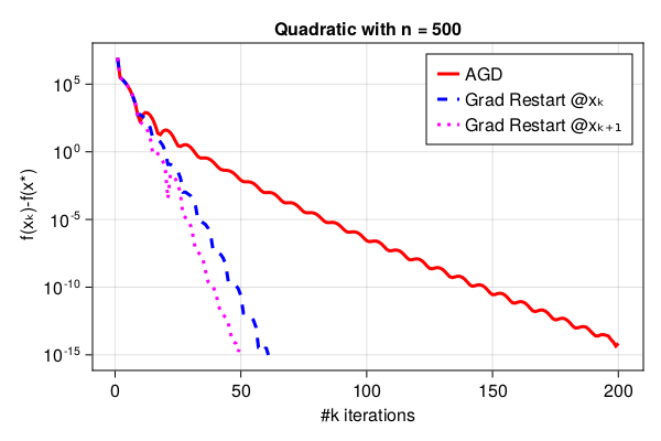
Figure 1: A Julia plot. A comparison of the performances of the restart scheme in Algorithm 1 at $x_{k+1}$ (the pink dotted curve), the restart scheme in [O’Donoghue and Candès(2015)] at $x_{k}$ (the blue dashed curve) and the classical AGD (the solid red curve) when applied to minimize simple quadratic.

We can see in Fig. 1 that keeping $x_{k+1}$ at the restart yields a modest improvement over keeping $x_{k}$. Our theory for the $n=1$ case required keeping $x_{k+1}$ rather than $x_{k}$.

Appendix E Huber Regression

Another numerical example is the following problem of Huber Regression. Define,

$$\psi_{\tau}(x)=\begin{cases}x^{2},&|x|\leq\tau\\ 2\tau x-\tau^{2}&x\geq\tau\\ -2\tau x-\tau^{2}&x\leq-\tau.\end{cases}$$ (43bh)

Given $A\in\R^{m\times n}$ and $y\in\R^{m}$ we consider the optimization problem,

$$\min_{x\in\R^{n}}\frac{1}{2}\sum_{i=1}^{m}\psi_{\tau}(a_{i}x-y_{i})$$ (43bi)

where $a_{i}$ is a row of $A.$ For this experiment we set $\tau=0.5$, $m=300,n=50,$ and $A$ and $y$ were randomly generated using a standard normal distribution.

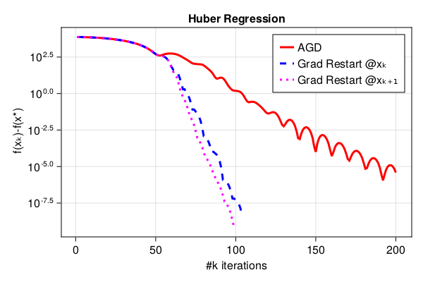
Figure 2: A Julia plot. A comparison of the performances of the restart scheme in Algorithm 1 at $x_{k+1}$ (the pink dotted curve), the restart scheme in [O’Donoghue and Candès(2015)] at $x_{k}$ (the blue dashed curve) and the classical AGD (the solid red curve) when applied to solve the Huber Regression problem.

In Fig. 2 it can be observed that restarting using $x_{k+1}$ offers slightly better performance.

Appendix F The Hinder-Lubin Example Expanded

Hinder and Lubin constructed a function [Hinder and Lubin(2020), Appendix D.4] for which the restarts of O’Donoghue and Candés performed poorly until the iterates of $(x_{k})_{k\in{\mathbb{N}}}$ were close to the minimizer. Their objective function is defined as

$$f(x)=\sum_{i=1}^{n}ih_{\delta}(x_{i})+\frac{\alpha}{2}||x||^{2}_{2},$$ (43bj)

where

$$h_{\delta}(z)=\begin{cases}z^{2}/2,&z\geq-\delta\\ -\delta z-\delta^{2}/2&z<-\delta.\end{cases}$$ (43bk)

Remark that $f:\R^{n}\rightarrow\R$ is $(n+\alpha)-$smooth and $\alpha$-strongly convex with a unique minimizer at $x=0.$ The function $f$ is also separable, and therefore one can apply Algorithm 1 along each coordinate. We see that the restart scheme of Algorithm 1 performs well. In most cases, we do not have knowledge of whether the function is separable or not but there are cases where running Algorithm 1 in parallel along each coordinate has merit. We introduce a modified function obtained from (43bj) that is not separable. Given a matrix $A\in\R^{m\times n}$, define

$$F(x)=f(x)+\gamma\sum_{i=1}^{m}\left(\left\langle{a_{i}},{x}\right\rangle+\sqrt{\left\langle{a_{i}},{x}\right\rangle^{2}+1}\right)$$ (43bl)

where $f$ is the Hinder and Lubin function defined in 43bj, $a_{i}$ are the rows of $A$, and $\gamma\in\R$. For the experiment we chose $m=110,n=100,$ and set $\delta=\alpha=\gamma=10^{-4}.$ Note that $F$ is now $\left(n+\alpha+\gamma\sum_{i=1}^{m}\norm{a_{i}}\right)-$smooth. In the experiment we compare AGD, AGD with the gradient restarts, and Algorithm 1 running along each coordinate.

Figure 3: A Julia plot. A comparison of the performances of the parallel gradient restart scheme using Algorithm 1 for each coordinate (the pink dotted curve), the restart scheme in [O’Donoghue and Candès(2015)] at $x_{k+1}$ (the blue dashed curve) and the classical AGD (the red curve) when applied to solve the modified Hinder-Lubin function 43bl. As the plots reflect, while the objective function is not separable, separate restarts still improve performance.

In Fig. 3 it can be seen that the gradient based restarts perform poorly until the iterates get close to the minimizer. On the other hand, restarting along each coordinate performs much better even though $F$ is not separable.

References

- [Alamo et al.(2019)Alamo, Krupa, and Limon] Teodoro Alamo, Pablo Krupa, and Daniel Limon. Gradient based restart FISTA. In 2019 IEEE 58th Conference on Decision and Control (CDC), pages 3936–3941, 2019. 10.1109/CDC40024.2019.9029983.
- [Aujol et al.(2023)Aujol, Calatroni, Dossal, Labarrière, and Rondepierre] Jean-François Aujol, Luca Calatroni, Charles Dossal, Hippolyte Labarrière, and Aude Rondepierre. Parameter-free FISTA by adaptive restart and backtracking. Arxiv preprint 2307.14323, 2023.
- [Bauschke and Moursi(2024)] Heinz H. Bauschke and Walaa M. Moursi. An Introduction to Convexity, Optimization, and Algorithms. Society for Industrial and Applied Mathematics, 2024.
- [Beck(2017)] Amir Beck. First-Order Methods in Optimization. Society for Industrial and Applied Mathematics, Philadelphia, PA, 2017. 10.1137/1.9781611974997. URL https://epubs.siam.org/doi/abs/10.1137/1.9781611974997.
- [Beck and Teboulle(2009)] Amir Beck and Marc Teboulle. A fast iterative shrinkage-thresholding algorithm for linear inverse problems. SIAM Journal on Imaging Sciences, 2(1):183–202, 2009. 10.1137/080716542. URL https://doi.org/10.1137/080716542.
- [Fercoq and Qu(2019)] Olivier Fercoq and Zheng Qu. Adaptive restart of accelerated gradient methods under local quadratic growth condition. IMA Journal of Numerical Analysis, 39(4):2069–2095, 03 2019. ISSN 0272-4979. 10.1093/imanum/drz007. URL https://doi.org/10.1093/imanum/drz007.
- [Giselsson and Boyd(2014)] Pontus Giselsson and Stephen Boyd. Monotonicity and restart in fast gradient methods. In 53rd IEEE Conference on Decision and Control, pages 5058–5063. IEEE, 2014.
- [Hinder and Lubin(2020)] Oliver Hinder and Miles Lubin. A generic adaptive restart scheme with applications to saddle point algorithms. Arxiv preprint 2006.08484, 2020.
- [Necoara et al.(2019)Necoara, Nesterov, and Glineur] I. Necoara, Yu. Nesterov, and F. Glineur. Linear convergence of first order methods for non-strongly convex optimization. Math. Program., 175(1):69–107, May 2019. ISSN 1436-4646. 10.1007/s10107-018-1232-1.
- [Nesterov(1983)] Yurii Nesterov. A method for solving the convex programming problem with convergence rate . Proceedings of the USSR Academy of Sciences, 269:543–547, 1983.
- [O’Donoghue and Candès(2015)] Brendan O’Donoghue and Emmanuel Candès. Adaptive Restart for Accelerated Gradient Schemes. Found. Comput. Math., 15(3):715–732, June 2015. ISSN 1615-3383. 10.1007/s10208-013-9150-3.