Cosmology from LOFAR Two-metre Sky Survey Data Release 2:
Angular Clustering of Radio Sources

Abstract

Covering $\sim$5600$\,\deg^{2}$ to rms sensitivities of $\sim$70$-$100 $\muup$Jy beam^-1, the LOFAR Two-metre Sky Survey Data Release 2 (LoTSS-DR2) provides the largest low-frequency ($\sim$150 MHz) radio catalogue to date, making it an excellent tool for large-area radio cosmology studies. In this work, we use LoTSS-DR2 sources to investigate the angular two-point correlation function of galaxies within the survey. We discuss systematics in the data and an improved methodology for generating random catalogues, compared to that used for LoTSS-DR1, before presenting the angular clustering for $\sim$900 000 sources $\geq$$1.5$ mJy and a peak signal-to-noise $\geq$$7.5$ across $\sim$$80\%$ of the observed area. Using the clustering we infer the bias assuming two evolutionary models. When fitting angular scales of $0.5\leq\theta<5\,\deg$, using a linear bias model, we find LoTSS-DR2 sources are biased tracers of the underlying matter, with a bias of $b_{C}=2.14^{+0.22}_{-0.20}$ (assuming constant bias) and $b_{E}(z=0)=1.79^{+0.15}_{-0.14}$ (for an evolving model, inversely proportional to the growth factor), corresponding to $b_{E}=2.81^{+0.24}_{-0.22}$ at the median redshift of our sample, assuming the LoTSS Deep Fields redshift distribution is representative of our data. This reduces to $b_{C}=2.02^{+0.17}_{-0.16}$ and $b_{E}(z=0)=1.67^{+0.12}_{-0.12}$ when allowing preferential redshift distributions from the Deep Fields to model our data. Whilst the clustering amplitude is slightly lower than LoTSS-DR1 ($\geq$2 mJy), our study benefits from larger samples and improved redshift estimates.

1 Introduction

The LOw Frequency ARray (LOFAR; van Haarlem et al., 2013) is a key radio telescope array, transforming views of the low-frequency radio skies. Based in Europe, its full array combines a dense core of stations in the Netherlands with additional stations that have much larger baselines both across the Netherlands and Europe. This allows baselines of up to $\sim 100\,\mathrm{km}$ across the Netherlands and $\sim 2000\,\mathrm{km}$ across Europe, producing 6″ resolution using the Dutch stations only and sub-arcsecond resolution imaging using the full array (Morabito et al., 2022; Sweijen et al., 2022), at $150\,\mathrm{MHz}$. These stations combine two types of antennas to operate in two low frequency ranges: the Low-Band Antennas (LBA; $10-80\,\mathrm{MHz}$) and High-Band Antennas (HBA; $120-240\,\mathrm{MHz}$). Such low frequency observations lead to a large field of view for each LOFAR observation, making it an excellent instrument for survey science. As part of this, LOFAR is currently focusing on several large-area survey projects, including: the LOFAR LBA Sky Survey (LoLSS; de Gasperin et al., 2021) and the LOFAR Two-metre Sky Survey (LoTSS; Shimwell et al., 2017, 2019, 2022) with the HBA, which is what we use for this work. LoTSS aims to observe the entire northern hemisphere at $144\,\mathrm{MHz}$ to a typical rms sensitivity of $\sigma_{144\,\mathrm{MHz}}\sim 70-100\,\muup\mathrm{Jy}\,\mathrm{beam}^{-1}$ and trace a combination of Active Galactic Nuclei (AGN) and Star-Forming Galaxies (SFGs) across large periods of cosmic time. At such frequencies, the dominant radiative mechanism is synchrotron emission from relativistic electrons spiraling in the magnetic fields. This leads to a typically power-law-like distribution for flux densities as a function of frequency ($S_{\nu}\propto\nu^{-\alpha}$) with a range of spectral indices, typically assumed to be $\alpha\sim 0.7-0.8$ for an average radio population (Kellermann et al., 1969; Mauch et al., 2003; Smolčić et al., 2017a; de Gasperin et al., 2018), though much larger or smaller values can be observed for individual sources with flat or peaked spectra (e.g. Massaro et al., 2014; Callingham et al., 2017; O’Dea & Saikia, 2021).

LoTSS has developed over a series of data releases, improving in properties such as angular resolution, sensitivity, image fidelity and areal coverage. Initially, observations covering $350\,\deg^{2}$ were released with direction-independent calibration only at a resolution of $25\,\arcsec$, detecting $\sim$44 000 sources with a typical noise of $\sim 0.5\,\mathrm{mJy}\,\mathrm{beam}^{-1}$. This was then improved upon in both resolution and sensitivity with the first fully direction-dependent calibrated data release for LoTSS: LoTSS-DR1 (Shimwell et al., 2019). This data release covered $424\,\deg^{2}$ over the The Hobby-Eberly Telescope Dark Energy Experiment (HETDEX) Spring Field (Hill et al., 2008) with a corresponding catalogue of $\sim$325 000 sources, with a 1$\sigma$ sensitivity of $\sim 70-100\,\muup\mathrm{Jy}\,\mathrm{beam}^{-1}$ at 6″ angular resolution. This sky coverage has now been enlarged in the latest data release, LoTSS-DR2 (Shimwell et al., 2022), which covers $\sim 5600\,\deg^{2}$ with an accompanying catalogue of $\sim 4.4$ million sources. This is the largest catalogue of radio sources within an individual radio survey to date. Such a combination of area and large source numbers means that LoTSS-DR2 provides an excellent dataset for radio cosmology studies, allowing for a more detailed understanding of the distribution of radio sources in the Universe.

The study of the distribution of sources observed in galaxy surveys throughout the Universe is important for a number of reasons. Most importantly, it allows us to understand more about how galaxies trace the large-scale structure of the Universe and the underlying dark matter distribution. Starting from initial primordial over-densities, dense regions of matter have come together and evolved over time. This has resulted in the large-scale distribution of matter we observe today (Colless et al., 2001; Doroshkevich et al., 2004; Springel et al., 2006). This coming together of dark matter forms haloes in these initially over-dense regions, and leaves an absence of dark matter, known as voids, in regions of initial under-densities. Filaments then connect dense regions together. Luminous matter, that we observe in astrophysical objects such as stars and galaxies, is also attracted together under the effects of gravity but is further influenced by factors such as the effect of feedback associated with both star formation and from active galactic nuclei (see e.g. Ceverino & Klypin, 2009; Hopkins et al., 2012; Fabian, 2012; Morganti, 2017). Since galaxies form in dense regions, they trace peaks in the underlying matter distribution, leading galaxies to be known as biased tracers of the matter distribution in the Universe (see e.g. Peebles, 1980; Kaiser, 1984; Mo & White, 1996; Desjacques et al., 2018).

On large scales, the galaxy overdensity, $\delta_{g}({\bf x},z)$, can be considered to trace the matter overdensity, $\delta_{m}({\bf x},z)$, related by a quantity known as “galaxy bias”, $b(z)$:

$$\delta_{g}({\bf x},z)=b(z)\,\delta_{m}({\bf x},z).$$ (1)

To quantify galaxy bias, a common method is to first determine the excess probability to observe galaxies within different spatial separations, compared to if they were randomly distributed. This is known as the spatial two-point correlation function, $\xi(r,{z})$. The redshift dependent linear bias, $b(z)$, can then be measured and is related to the ratio of spatial clustering of galaxies, $\xi(r,{z})$, to the clustering of matter, $\xi_{M}({r,z})$, as given by:

$$b^{2}{(z)}=\frac{\xi_{{g}}(r,z)}{\xi_{{M}}(r,z)}.$$ (2)

The spatial clustering of galaxies, $\xi_{g}(r)$, defines the excess clustering of galaxies observed at a given spatial separation, compared to if they were randomly distributed. Such measurements of the spatial clustering rely on accurate redshifts and corrections due to peculiar velocities. Where highly accurate redshifts are not available for sources in a survey, it is still possible to estimate the spatial clustering by combining the observed projected angular clustering of sources with their redshift distributions using methods such as Limber inversion (Limber, 1953, 1954). Radio surveys provide excellent catalogues to measure the large-scale structure of the Universe as they predominately trace extragalactic sources over a broad redshift range and over large areas, but typically rely on angular clustering measurements instead of spatial measurements.

The angular two-point correlation function ($\omega(\theta)$, see e.g. Totsuji & Kihara, 1969; Peebles, 1980; Cress et al., 1996; Blake & Wall, 2002; Overzier et al., 2003; Wang et al., 2013) does not rely on redshifts for its calculation and quantifies the excess probability ($dP$) of pairs of sources observed within a survey catalogue at a given projected angular separation, $\theta$, compared to if the sources were randomly distributed on the sky, with no intrinsic large-scale structure. This is defined by:

$$dP=N\left[1+\omega(\theta)\right]d\Omega,$$ (3)

where $d\Omega$ is the solid angle of the observations and $N$ is the mean number of sources per unit area.

Radio continuum surveys rely on multi-wavelength information for redshifts (see e.g. Smolčić et al., 2017b; Prescott et al., 2018; Algera et al., 2020), which are typically dominated by less accurate photometric redshifts for a large fraction of the sources. For LOFAR, in the first LoTSS data release (Shimwell et al., 2019), sources were cross-matched to sources in surveys such as Pan-STARSS (Chambers et al., 2016) and WISE (Wright et al., 2010; Williams et al., 2019), with $\sim$50% of LoTSS-DR1 sources having redshift information (see Duncan et al., 2019). Similarly for the LoTSS Deep Fields, the wealth of multi-wavelength data has been used to obtain redshifts for 97% of sources across the multi-wavelength defined regions in the three fields LoTSS Deep Fields (see Sabater et al., 2021; Tasse et al., 2021; Kondapally et al., 2021; Duncan et al., 2021) which was used to help classify such sources (see Best et al., 2023). The accuracy of redshifts for such radio sources will be improved upon with future spectroscopic surveys (such as WEAVE-LOFAR; Smith et al., 2016).

Combining measurements of the angular clustering and redshift distribution, the spatial clustering for a population of sources can be inferred. The spatial clustering can then be used to estimate the galaxy bias of radio sources (as in Equation 2), this will be discussed further in Section 5. Such clustering and bias measurements have been presented in a number of works (see e.g. Magliocchetti et al., 1999; Magliocchetti et al., 2004; Negrello et al., 2006; Lindsay et al., 2014a; Nusser & Tiwari, 2015; Magliocchetti et al., 2017; Hale et al., 2018; Siewert et al., 2020; Tiwari et al., 2022; Mazumder et al., 2022). A number of such studies suggest an evolving bias model for radio sources, suggesting radio sources are more biased tracers of the underlying matter distribution at higher redshift. Moreover, studies which further consider the bias for radio SFGs and AGN separately have shown that these sources have different bias distributions and trace different mass haloes (see e.g. Magliocchetti et al., 2017; Hale et al., 2018; Chakraborty et al., 2020; Mazumder et al., 2022). Such studies have shown that AGN appear to inhabit more massive haloes than for SFGs at similar redshifts, reflecting the fact that they preferentially inhabit massive ellipticals. Further studies which classify AGN suggest that the haloes hosting radio AGN may be related to the accretion mode of AGN (using high redshift analogues to high/low excitation radio galaxies, see Hale et al., 2018). Such differences in the bias of different source populations can be advantageous for cosmological analysis, using the multi-tracer techniques (see e.g. Ferramacho et al., 2014; Raccanelli et al., 2012; Gomes et al., 2020). These techniques require understanding of the bias evolution for different source populations and make use of such difference to help place constraints on, for example, non-Gaussianity.

Further cross-correlating radio data with other cosmological tracers (see e.g. Allison et al., 2015; Alonso et al., 2021) can also help remove some of the systematics which remain in the data and have added further constraints on the galaxy bias evolution of radio sources, and Alonso et al. (2021) further used this to place constraints on the redshift distributions for radio sources, where no redshift information was available. Measurements of bias have been used in numerous studies to relate such measurements to the typical mass of the dark matter haloes which are hosting such sources (see e.g. those described in Mo & White, 1996; Tinker et al., 2010), but there are caveats to such measurements, especially if full halo occupation models are not taken into account (see e.g. Aird & Coil, 2021).

In this paper, we investigate the angular clustering of radio sources within $\sim 4500\,\deg^{2}$ of the LoTSS-DR2 survey and use this to infer the average bias of LoTSS-DR2 sources. The paper is arranged as follows: in Section 2 we describe the LoTSS-DR2 data used in this analysis, as well as the methods to measure the angular clustering of radio galaxies in Section 3. This includes a detailed description of the methods used in order to obtain accurate random sources that mimic the distribution of observational biases across the field of view, which develops the techniques used for LoTSS-DR1 (Siewert et al., 2020). Then, in Section 4 we present our measurements of the angular clustering of sources and our validation of these measurements before presenting our methods to determine galaxy bias in Section 5. This allows us to place constraint on how such sources trace the underlying matter and dark matter haloes across cosmic time. We then discuss our results in Section 6. We then go on to draw final conclusions in Section 7. For this paper we assume standard cosmological parameters from Planck Collaboration et al. (2020) in a flat model Universe, specifically: $H_{0}=67.4$ km s^-1 Mpc^-1, $\Omega_{b}$=0.0493, $\Omega_{c}$=0.264, $\Omega_{m}=\Omega_{b}+\Omega_{c}$, $\Omega_{\Lambda}=1-\Omega_{m}$, $n_{s}$=0.965, $\sigma_{8}$=0.811, unless otherwise stated.

2 Data

For this work we make use of the data and associated data products from two LOFAR survey projects: (i) the large area LoTSS-DR2 survey (Shimwell et al., 2022) and (ii) the associated redshift information from sources in the smaller LoTSS Deep fields (Duncan et al., 2021).

2.1 LoTSS-DR2

The majority of data used in this work consists of images and catalogues from the mosaics generated from combining 841 individual pointings of LoTSS-DR2 (Shimwell et al., 2022) covering $\sim$5600$\,\deg^{2}$ over two regions. The first of these is centered at 13h in RA, covering $4178\,\deg^{2}$, and the second region is centred at an RA of 1h, covering $1457\,\deg^{2}$. The data were reduced in a two stage process which consists of both a direction-independent and a direction-dependent calibration pipeline. The former flags, calibrates and averages the data in order to reduce the large data volumes, whilst the latter does further calibration and imaging to account for direction-dependent effects. This includes the effect of the varying ionosphere across the field of view, which is more prominent at the observing frequencies that telescopes such as LOFAR operate at, compared to higher-frequency radio observations. As presented in works such as van Weeren et al. (2016); Williams et al. (2016); Shimwell et al. (2019); Tasse et al. (2021), such direction-dependent calibration of LOFAR data is crucial for improving image fidelity and for producing higher resolution imaging of the field at 6″ angular resolution, compared to 25″ without this accounted for (see e.g. Shimwell et al., 2017), when using only the Dutch LOFAR stations. Source catalogues were generated using the source finder PyBDSF (Mohan & Rafferty, 2015) which detected a total of $\sim$4.4 million sources across the full LoTSS-DR2 coverage. The distribution of these sources over the northern hemisphere can be seen in Figure 1. This distribution varies significantly across the field of view due to a combination of factors. These include intrinsic large-scale structure, and non-uniform detection across the field of view resulting from instrumental, calibration and source finding effects. Understanding the factors which cause such non-uniformity in the data is important in order to accurately measure the true angular clustering of sources and will be discussed further in Section 3.2. Unless otherwise stated, any mention of images and pointings from LoTSS-DR2 refer to the mosaic images which are available from https://lofar-surveys.org, and are the mosaiced region closest to the pointing centre.

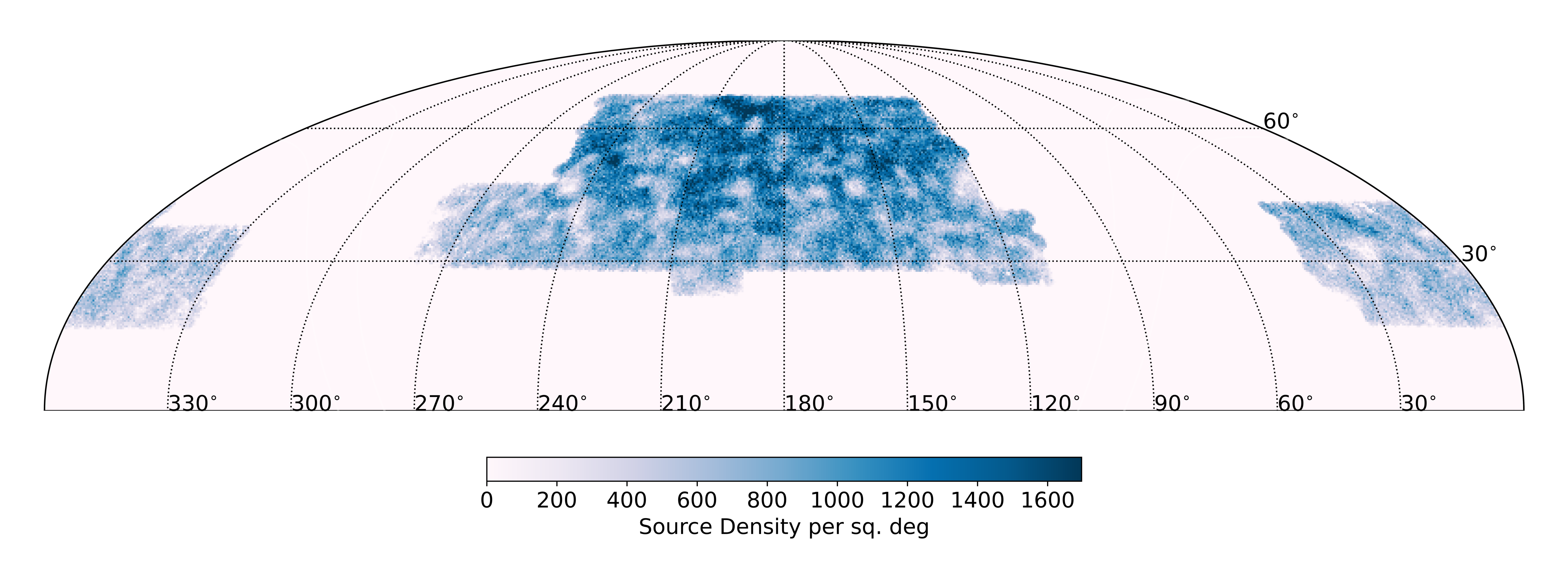
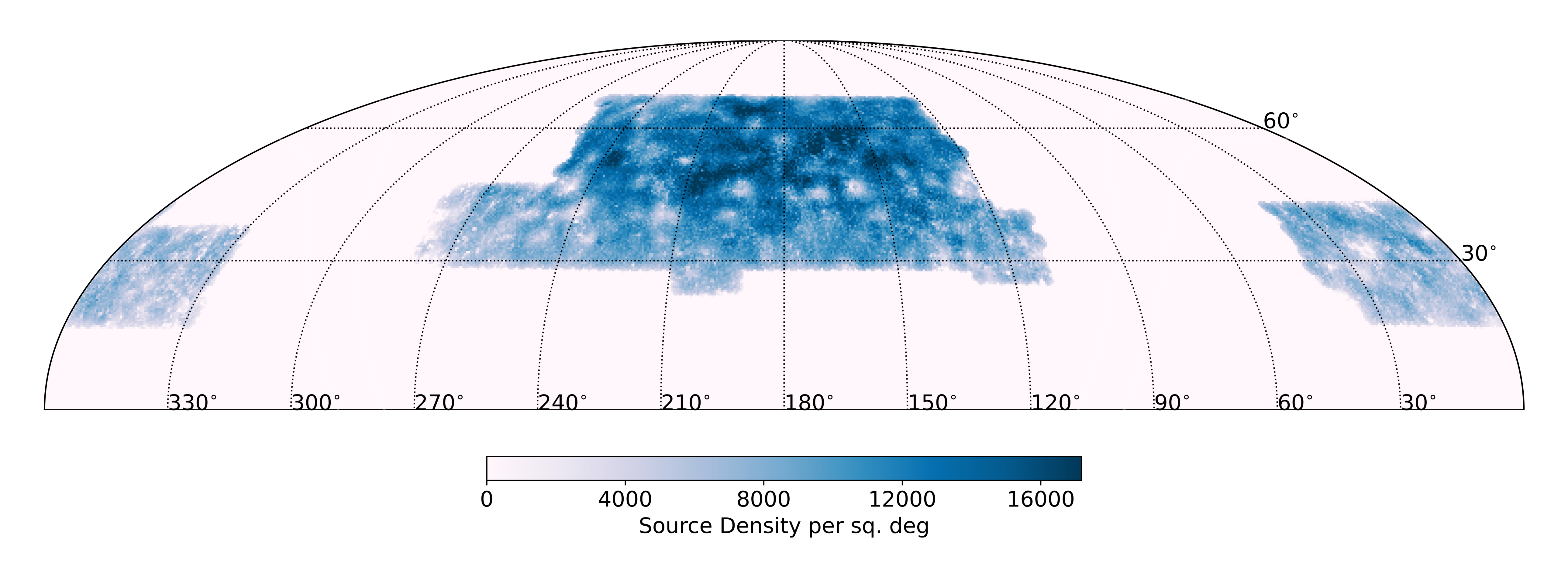
Figure 1: Sky density distribution of all sources in the LoTSS-DR2 survey (upper) from Shimwell et al. (2022) and for the random catalogues generated for this work (lower; prior to any flux density, SNR or spatial cuts). This shows the two large regions covered by the survey, centred on right ascensions of 1h (15 $\deg$) and 13h (195 $\deg$). The figure is plotted in the Mollweide projection using HealPix (Górski et al., 2005; Zonca et al., 2020) with an N${}_{\textrm{side}}$=256. The colour scale indicates the source density per sq. $\deg$ across the field of view.

2.2 LoTSS Deep Fields

In order to relate any observed angular clustering to the spatial clustering and bias, it is crucial to have knowledge of the redshift distribution of the sources within the field. As there are not direct measurements of redshifts for the full population of LoTSS-DR2 sources we make use of the LoTSS Deep Fields data (Sabater et al., 2021; Tasse et al., 2021) which targets a handful of fields in the northern hemisphere with an abundance of multi-wavelength data, these are observed to deeper sensitivities than in LoTSS-DR2. Observations within these fields are important to help infer the redshift distribution of the sources observed within LoTSS-DR2. The first LoTSS Deep Fields data release consisted of three fields: Boötes, Lockman Hole and the European Large-Area ISO Survey Northern Field 1 (ELAIS-N1) field. These were observed for a total of 80, 164 and 112 hours respectively, covering $\sim 20\,\deg^{2}$ in each field.

For each field, a smaller region was defined for which there exists deep multi-wavelength information. In such regions, the source catalogues from PyBDSF were cross-matched to host galaxies (Kondapally et al., 2021) using a wealth of ancillary data. This cross-matched area constituted a total area of $8.6\,\deg^{2}$ in the Boötes field, $6.7\,\deg^{2}$ in ELAIS-N1 and $10.3\,\deg^{2}$ in the Lockman Hole field, totalling $25.6\,\deg^{2}$ across the three fields. For the cross-matched sources, a redshift was also associated to the source using a combination of template fitting to the multi-wavelength data as well as machine learning methods in order to obtain probability density functions (PDFs) for the redshift distributions, denoted $p(z)$. A ‘best redshift’ was then assigned to each source based on the PDF, or a spectroscopic redshift if such was available for the sources. More detail on this can be found in Duncan et al. (2021). We use these redshift distributions to estimate the redshift distribution, $p(z)$, for sources in the wider LoTSS-DR2 survey. This will be discussed further in Section 5.1.

3 Angular clustering and Randoms Generation

3.1 Angular Clustering

As discussed in Section 1, one way to investigate the clustering of sources within a galaxy catalogue is through measuring the angular two point correlation function (TPCF) , denoted by $\omega(\theta)$. The TPCF quantifies the excess clustering observed at a given angular separation in the catalogue data, compared to what would be observed over the field of view if there was no large-scale structure within the data. Naively, such excess probability to detect galaxies in the data at a given angular separation compared to the distribution from random sources is given by:

$$\omega(\theta)=\frac{\overline{{DD}}(\theta)}{\overline{{RR}}(\theta)}-1.$$ (4)

In this estimator, $\overline{DD}(\theta)$ is the counts of pairs of galaxies within the data catalogue at a given angular separation $\theta$ (normalised such that $\Sigma_{\theta}\overline{DD}(\theta)=1$) and $\overline{RR}(\theta)$ is the corresponding normalised pair counts within a random catalogue. This random catalogue is generated to mimic observational effects across the field of view. If the data were indeed randomly distributed and exhibited no large-scale structure behaviour, $\omega(\theta)$ would fluctuate around a value of 0. Any deviation from this suggests intrinsic large-scale structure. A number of predictions for galaxies as well as observations have suggested that this angular clustering behaves as a power law for galaxies and specifically radio sources (see e.g. Peebles, 1980; Blake & Wall, 2002; Lindsay et al., 2014a; Magliocchetti et al., 2017, but see Section 4). Whilst Equation 4 could be used to estimate $\omega(\theta)$, work by Landy & Szalay (1993) has shown that a more accurate estimator of $\omega(\theta)$ is given by

$$\omega(\theta)=\frac{\overline{{DD}}(\theta)-2\overline{{DR}}(\theta)+\overline{{RR}}(\theta)}{\overline{{RR}}(\theta)}.$$ (5)

In this estimator, $\overline{DR}(\theta)$ is the corresponding normalised pair counts between the data and random catalogues within a given angular separation. This estimator has been shown to have minimal variance and be less biased than other estimators such as Equation 4 (see Landy & Szalay, 1993). As such, we use Equation 5 to calculate $\omega(\theta)$ in this work.

To calculate $\omega(\theta)$, a random catalogue must first be generated to compare to the data. If source detection across the field of view were uniform, such a random catalogue could be generated through sampling random positions across the observed field of view. However, the detection of sources is not uniform (see Figure 1) and will be affected by a number of observational effects across the sky. Thus, the generation of randoms which accurately mimic the detection of sources across the sky is crucial to avoid observational effects being mistaken for intrinsic large-scale structure. We therefore employ a number of methods (discussed in Section 3.2) to mimic such observations across the field of view.

To measure $\omega(\theta)$, we make use of the package TreeCorr (Jarvis, 2015) to calculate the pairs of galaxies within angular separation bins that are uniformly spaced bins in $\ln(\theta)$ and cover the range of angular scales possible with the data. Due to the large area coverage of LoTSS-DR2, we ensure that the metric for calculating separations within TreeCorr is set to ‘Arc’. This helps to more accurately calculate separations across large fields of view, using great circle distances. We also set the parameter bin_slop to $0$ which enforces that exact calculations are made to calculate the number of pairs of sources within each angular separation bin, as opposed to the default method which has some flexibility between the separation bins in order to help speed up the calculation of pairs. Such parameters were determined to be important in the work of Siewert et al. (2020), where a non-zero bin_slop was found to introduce larger errors in the measurement of $\omega(\theta)$. The associated uncertainties in $\omega(\theta)$ will be discussed in greater detail in 3.4 and its connection to linear bias also discussed in Sections 5.2-5.3.

3.2 Randoms

As discussed in Section 3.1, in order to measure the angular clustering from LoTSS-DR2 we need to have a catalogue of random sources which mimics the detection of data across the field of view. Figure 1 highlights the non-uniform detection of radio sources across the field of view, due to a combination of factors including sensitivity variations across the field of view due to bright sources, reduced sensitivity with declination and smearing of points sources across the field of view. In building our random catalogue we will take a series of steps to account for these effects. An outline of these steps, as well as the section in which these shall be applied is as follows:

1. Survey Area - we generate randoms across the survey field of view, ensuring we remove any masked regions within pointings which are masked out due to failures within the data reduction process. We consider this in Section 3.2.1.

2. Smearing - There may be position-dependent smearing effects across the field of view of a pointing, as well across the 5600 sq. deg. Smearing will affect the detection of sources (which is based on signal-to-noise ratio ‘SNR’, defined here as peak flux density/rms (root mean square noise), for which the Isl_rms column is used for rms of the data), and could arise from effects such as residual calibration uncertainties and uncorrected smearing effects inherent to the data averaging. We model smearing across the field of view and its dependence on field elevation and correct for this, which is discussed in Section 3.2.2.

3. Incompleteness and measurement errors - The sensitivity (rms) will vary across the survey area, such as with elevation or declination (see Fig. 2 of Shimwell et al., 2019) or location within the mosaic and proximity to bright sources, where the noise is known to be elevated. Variations may also exist towards the edge of the field, where there are fewer neighbouring pointings that can be mosaiced together (as mosaicing would reduce the noise). This will affect source detection and hence the completeness. Furthermore, the source finder may have a completeness dependence with SNR and its measurement errors can affect the properties such as flux density associated with sources. We account for completeness as a function of source input SNR and the effect that noise and the source finder may have on the measured flux properties of sources in Section 3.2.3.

4. Additional spatial masking - Finally, there may be additional spatial regions which should be masked to avoid regions such as the unmosaiced edges of pointings; this is described in Section 3.3.

We note, though, that there may be limitations to generating the randoms which may be more challenging to account for, especially over the large area of LoTSS-DR2. This includes residual primary beam uncertainties which are unknown and that mosaicking pointings together may cause additional smearing which can very spatially due to pointing dependent astrometric offsets. To minimise the effects of these, additional flux limit and SNR limits can be applied to both the data and random samples. Specifically, for our final analysis we limit the sample to $\geq$1.5 mJy and $\geq$ 7.5$\sigma$. We discuss these and additional cuts in Sections 3.3.2 - 3.3.3.

3.2.1 Input Simulated Catalogue

The first step in generating accurate random catalogues for the LoTSS-DR2 survey is to generate a sample of input positions which are uniformly distributed across the field of view of LoTSS-DR2, accounting for masked regions within the fields. For this work, we generated random positions in the range: RA from 0^∘ to 360^∘ and Dec from 20^∘ to 80^∘. This wide area encompasses the full LoTSS-DR2 footprint, but a significant fraction of such a region is not covered by LoTSS-DR2. Therefore, we use the associated rms maps of each individual pointing to identify the sources within the LoTSS-DR2 area. We assign each random position an rms value, based on the pixel value at the source location, using the rms map for the closest pointing. This also allows sources within masked regions, or regions not surveyed in LoTSS-DR2 to be identified. Random sources falling within the surveyed region are retained and consist of $\sim 200$ million input simulated positions across the field of view of LoTSS-DR2.

To account for sensitivity variations and the effect that this has on the detection of sources, we take a number of iterative steps. Firstly, we assign simulated properties of radio sources to each of the $\sim 200$ million random positions. Such properties include the flux density of the simulated source, as well as source shape information. To do this, we make use of the SKA Design Studies Simulated Skies (hereafter SKADS Wilman et al., 2008; Wilman et al., 2010), which provide a simulated catalogue of sources covering $100\,\deg^{2}$ with multiple observable properties for each simulated source. These properties include an associated redshift, flux density measurements at several frequencies in the range $151\,\mathrm{MHz}-18\,\mathrm{GHz}$, shape information and source type (e.g. AGN or SFG). Recent observations suggest that SKADS underestimated the number of SFGs at the faintest flux densities (see e.g. Bonaldi et al., 2016; Smolčić et al., 2017a; van der Vlugt et al., 2021; Matthews et al., 2021; Hale et al., 2023; Best et al., 2023). Therefore, we employ a modified version of the SKADS catalogue where the number of SFGs in the original catalogue are doubled, as also done in Hale et al. (2023). The source counts from the modified SKADS catalogue better reflects deep data from the LoTSS Deep Fields (Mandal et al., 2021), source counts presented for LoTSS-DR2 (Shimwell et al., 2022) and data from other wavelengths scaled to $144\,\mathrm{MHz}$, assuming a spectral index of $\alpha=0.7$, We initially use a minimum flux density of $0.1\,\mathrm{mJy}$ for the SKADS sources to validate the randoms, but increase this to $0.2\,\mathrm{mJy}$ once flux density cuts are applied (see Section 3.3.2). We note that the relatively limited area of SKADS compared to LoTSS-DR2 means that the contribution of the much rarer, bright sources may be undersampled and so may differ from LOFAR observations. However such bright sources are rare in the observations and simulations and so will not contribute largely to the clustering. Moreover, those sources will not be sensitivity limited. Due to the nature of the large area of LoTSS-DR2, SKADS sources will need to be repeated in our random sample, to ensure both spatial coverage and to allow the random sample to be significantly larger than the data. Whilst other simulated radio catalogues exist, such as T-RECS (Bonaldi et al., 2019; Bonaldi et al., 2023), we will demonstrate later that the source counts used from this modified SKADS model can accurately represent the source counts of our data and other deeper observations, and have been shown to be successful in estimating completeness in other studies (Hale et al., 2023). Therefore, we feel we are able to adopt SKADS for use in this work. With future studies which split by source type and redshift, it will become increasingly important to use simulated catalogues which both have overall flux distributions which reflect the data as well as reflect the evolving luminosity functions for different populations.

As PyBDSF relies on peak SNR in order to determine whether a source is detected above the local noise, we need a peak flux density for the simulated sources. For a given integrated flux density, a point source is more likely to be detected than an extended source, due to the decreasing peak SNR for more extended sources. To assign a peak flux density to our simulated sources, we use the component catalogue which corresponds to the modified SKADS catalogue. The catalogue used for this work has a flux density limit of $5\,\muup\mathrm{Jy}$ at $1.4\,\mathrm{GHz}$ ($\sim 25\,\muup\mathrm{Jy}$ at $144\,\mathrm{MHz}$), and includes the shapes and orientations of components that make up the individual sources in the SKADS catalogue. Following Hale et al. (2021, 2023), we model each SKADS source through combining the emission related to the modelled components of a source. For each component, we model this as an ellipse randomly positioned within a pixel of the same pixel scale as the LOFAR observations. We convolve this ellipse with a Gaussian kernel representing the restoring beam which is an approximation to the point spread function (PSF) of the LOFAR observations (6″) and sum these components together. This procedure provides an input catalogue of sources which have information on the integrated flux density, redshift, source type and peak flux density, which we can assign to our random catalogues. Unlike in Hale et al. (2021, 2023), though, we do not inject sources into the images and re-extract sources using the source finder, PyBDSF. This is due to the large area of the field being considered, for which a significant computational effort would be required to create sufficient random sources to measure the clustering. Instead we make use of information from the simulations performed in Shimwell et al. (2022) to account for incompleteness across the sky. However, we must firstly account for smearing across the field of view.

3.2.2 Smearing

Smearing effects can reduce the peak flux densities of sources, and hence their detection. This smearing can originate from a range of factors including: bandwidth and time smearing (Bridle & Schwab, 1999); residual calibration errors; the size of the facets used in the reduction; and residual effects from the ionosphere interacting with the radio signals. The first of these, bandwidth and time smearing, is described in detail in Bridle & Schwab (1999) and is related to the averaging of data, which causes an increasing smearing with distance from the pointing centre. In LoTSS-DR1, Shimwell et al. (2019) suggested that the use of DDFacet reduced the effects of such smearing at the largest angular separations compared to Bridle & Schwab (1999) (see Fig. 10 of Shimwell et al., 2019). This is because DDFacet uses a different PSF in each facet which can be used to account for smearing in the data. The 6″restoring beam of LOFAR images is then used uniformly across the images. However, such a process leads to residual effects. For example, sources which are not fully deconvolved may still exhibit smearing and as only one PSF per facet is assumed, this can also lead to residual effects. We do not adopt the relation for smearing as presented in Fig 10 of Shimwell et al. (2019), but instead investigate the smearing for the LoTSS-DR2 data and how it varies with observational properties.

Given the large survey area of LoTSS-DR2 ($\sim$5600$\,\deg^{2}$), we consider whether there is a possibility of smearing being a function of position across the survey, in particular with the elevation of the observations, as the primary beam size of an individual pointing increases at low elevation with LOFAR as it is not a steerable telescope, and as there are larger ionospheric effects, because more of the Earth’s atmosphere is along the line of sight. This leads to larger and more elongated PSF sizes and observational area at lower declination (see LOFAR observations at lower declinations in Hale et al., 2019). Therefore, we consider the dependence of the observed smearing as a function of these parameters.

To investigate the relationship of the position-dependent smearing we make use of sources from the Faint Images of the Radio Sky at Twenty-cm survey (FIRST; Becker et al., 1995; Helfand et al., 2015) where we have overlap between the two surveys (mostly in the 13h field). FIRST is a 1.4 GHz survey with the VLA which observed the northern sky to $\sigma_{1.4\textrm{GHz}}\sim 0.15\,\mathrm{mJy}$ at 5″ resolution. To study the smearing, it is important to identify sources which are believed to be unresolved. Such sources should have a ratio of integrated to peak flux densities ($\frac{S_{I}}{S_{P}}$) of 1, though scatter will exist due to the effects of noise at lower signal-to-noise (SNR). Due to the higher angular resolution in FIRST compared to LoTSS-DR2, we make the assumption that those sources which are unresolved in FIRST will also be unresolved in LoTSS-DR2. To identify unresolved sources in FIRST, we took those which are isolated (no neighbours within 12″) and are high signal-to-noise (SNR$\geq$10). For those sources we follow the methods of previous works such as Smolčić et al. (2017a); Shimwell et al. (2019); Hale et al. (2021) and use a 95% SNR envelope of the form:

$$\frac{S_{I}}{S_{P}}=A\pm B\times\textrm{SNR}^{-C},$$ (6)

Figure 2: SNR envelope for integrated to peak flux density ratio as a function of SNR that is determined for isolated, high SNR sources in FIRST (see Section 3.2.2) Sources in blue are considered to be unresolved and in red are resolved. The model for the envelope is also provided.

where the $\pm$ reflects the upper/lower envelopes. $A$ is found using the value of $\frac{S_{I}}{S_{P}}$ at high SNR, and sources with $\frac{S_{I}}{S_{P}}$ below $A$ are used to fit for $B$ and $C$ in order to define the envelope. The form of the envelope fit for these sources can be seen in Figure 2. Those FIRST sources which are below the upper envelope are considered to be unresolved. These unresolved FIRST sources are then cross-matched within a 3″matching radius to LoTSS-DR2 sources which are isolated (again, within 12″), high-SNR sources (Eddington, 1913, SNR$\geq$20, to ensure sources are less affected by Eddington bias, see), and those sources which were considered single sources by PyBDSF (i.e. S_Code=‘S’).

We then consider the position-dependent median ratio of the integrated-to-peak flux densities as a function of distance to the nearest pointing centre and its dependence on RA, Dec and mean elevation of the field observation. Only those separation bins that have at least 200 sources within them are presented in Figure 3 and errorbars are generated by bootstrap resampling the sources within the bin 100 times after resampling one third of the sources.

Figure 3: The measured integrated to peak flux density ratio (an indicator of source smearing, y-axis) as a function of separation from the closest pointing centre (x-axis). The dependence of such smearing is shown as a function of declination (left), RA (centre) and elevation (right). The dashed-dot line in the right hand panel indicates the elevation dependent smearing model which will be used in this work. For elevation bins $\leq$65^∘ a constant model is used (green, orange and red data).

Figure 3, shows an increase in smearing across the field of view as a function of distance from the pointing centre. However, there is also an apparent dependence on the declination and elevation of the field. The relationship with the right ascension of the observations is more complicated. If we first consider the effects of declination, the median flux density ratios appear to increase with declining declination, whilst for the two lowest declination bins considered there is similarity in the trend of the observed smearing as a function of separation. If we consider the dependence on RA this does not appear to have a clear trend, but at the largest RA considered the smearing is minimized. However, we note that the comparison with FIRST does not have sufficient RA coverage to investigate the full RA range observed with LOFAR. Finally, if we investigated the elevation dependence of this smearing, we see increasing smearing with distance from the pointing centre, which also appears to decrease with elevation above an elevation of $\geq 65^{\circ}$, and to be constant at elevations below this. As the elevation of an observation is related to the declination of the source combined with the time of observation, such smearing effects are likely correlated. For this work we only consider the elevation-dependent smearing to correct the peak flux densities of the random sources, using for a model of the form:

$${\frac{S_{I}}{S_{P}}=C_{1}+e^{-D_{1}\times\theta}},$$ (7)

where $\theta$ is the angular separation (in degrees) from the pointing centre of the nearest pointing and $C_{1}$ and $D_{1}$ are values to be fit. We calculate the best fit values of $C_{1}$ and $D_{1}$ in bins of elevation and then model the average distribution of these parameters using a linear equation:

$${C_{1}=\alpha_{C}+\beta_{C}\times\epsilon,}$$ (8)

and similarly for $D_{1}$. Here $\alpha_{C}$ and $\beta_{C}$ are constants, and $\epsilon$ is the mid point of the elevation bin in degrees. These are fit for elevation bins with an elevation $\geq$60^∘. For those elevations $\leq 62.5$^∘ we apply the same relation to that fit for the 60-65^∘elevation range. These models are presented in Figure 3. When applied to the random sources, angular separations are measured to the nearest pointing centre and the mean elevation is taken as that of the nearest pointing. As can be seen from Figure 3, this functional form appears to be a good visual fit to the data. This smearing shows that for those sources at the largest angular distances from the pointing centre have greater smearing and so would be less easy to detect than for a source with the same integrated flux density close to the pointing centre.

3.2.3 Correcting the Simulations for Completeness and Source Measurement Effects

Once we have information for the flux density properties (both integrated and peak) for each simulated source, we consider the likelihood a random source would be detected, accounting for completeness. Due to the variations in rms across the image and the source finder itself, the completeness will vary across the sky and not all sources with intrinsic peak flux densities above 5$\sigma$ will be detected by the source finder, and some source with intrinsic SNR below the threshold will be pushed above the threshold. It is then important to use this understanding of the completeness variation to determine which of our simulated randoms would be detected if they were observed through the LoTSS-DR2 survey.

To measure this, we make use of the image plane completeness simulations which were presented and used in Shimwell et al. (2022) and investigate the recovery of sources over a range of flux density and source shapes. We use the output from these simulations in order to investigate completeness and the source counts for the survey. These simulations involved generating 10 simulated images for each field in which sources of varying flux densities and shapes are injected within the residual images of the individual pointings. This uses a source counts model from Mandal et al. (2021) to determine the number of sources to inject into a field. PyBDSF is then used to re-extract the sources over the simulated images. This then allows the completeness to be measured, which is presented as a function of flux density in Shimwell et al. (2022) for both point source completeness and using simulations which include extended sources, which we use for this work. These simulations can help quantify which of our simulated sources are likely to be detected, but also to establish what the “measured” flux densities of these sources may be, if they had theoretically been detected by the source finder. It is with a combination of accounting for these two effects that we generate our random catalogue of simulated sources.

Whilst the completeness is shown to have a large variation as a function of flux density for each LoTSS pointing (see Shimwell et al., 2022), the scatter is greatly reduced when its dependence on SNR is considered (see Figure 4). This smaller scatter is due to the fact that source finding with PyBDSF uses thresholding which is based on the peak flux density of pixels within a source, compared to the local noise, i.e. SNR. Both the boundary of pixels which contribute to a source island and the criteria which define which sources contribute to the catalogue both use a SNR threshold. This is a 3$\sigma$ and 5$\sigma$ thresholding limit respectively for the two criteria defined. Therefore, while the rms values vary between the different fields of LoTSS-DR2, so each field has a different flux density dependence on completeness, the SNR dependence is more likely to be consistent across the fields. This can be seen in the inset of Figure 4 which also demonstrates that at a 5$\sigma$ limit, which is used to generate the source catalogue, the completeness is in fact only $\sim$50%, rising to $\sim$95% at 7$\sigma$. Due to this consistency between fields, we therefore believe that using completeness as a function of SNR is a much more appropriate way to resample our simulated sources, instead of using solely a flux density dependence.

However, it is possible that while the average completeness as a function of SNR is consistent across the fields, it may be that completeness has both a dependency on SNR and flux density. This is because the intrinsic size distribution of sources is likely to have a dependence on flux density, such as AGN (which may have jets and be resolved) are likely to be brighter than star forming galaxies. For extended sources, these may be more likely to be detected at a given peak SNR as the larger sizes means that while the peak of the sources may be affected by a noise trough, pushing it below a detection limit, but the large size means that other neighbouring pixels could push the source above the detection limit, making it detectable. For smaller sources, they may be less likely to have a pixel above the detection threshold, given the smaller size. Therefore we also consider the flux density dependence of the completeness as a function of SNR (Figure 4). As can be seen in Figure 4, there does appear to be a weak flux density dependence of the completeness for the same SNR. For example at 5$\sigma$, there is a variation in completeness from $\sim$0.3 at $\sim$0.2 mJy to $\sim$0.65 at $\sim$5 mJy. This behaves in the way expected, as discussed above, with larger sources better detected. However, at $\sim$6-7$\sigma$ for sources with the highest flux densities considered in Figure 4 there is the opposite behaviour, where the completeness appears to decrease with increasing flux density of the simulated sources.

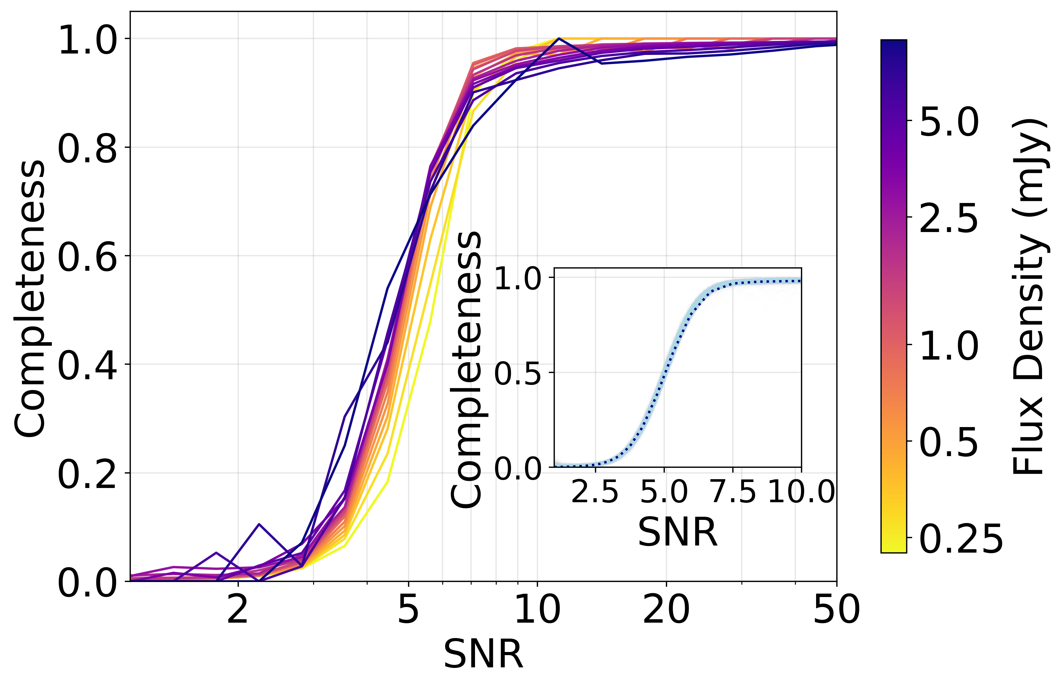
Figure 4: Completeness as a function of peak SNR (x-axis) and as a function of flux density (see colourbar) for sources across the 841 pointings of LoTSS-DR2. Inset: the completeness as a function of SNR only for each individual field (light blue) and the average across all fields (navy, dotted).

Moreover, the simulations from Shimwell et al. (2022) allow us to also consider (i) the combined effects of Eddington bias (Eddington, 1913), where faint sources are preferentially boosted to higher flux densities, and (ii) source finder measurement errors. Combined, this allows sources which would be inherently fainter than 5$\sigma$ to be detected by PyBDSF but leads to sources at lower SNR to have measured integrated and peak flux densities at values different to their intrinsic values. Hence, we also consider the ratio of the measured to input flux density for each simulated source as a function of input SNR. This is shown for both the integrated and peak flux densities in Figure 5. As can be seen, at high SNR, the measured-to-input flux density ratio tends to a value of 1, indicating that these sources can be accurately characterised by the source finder. At lower SNR there is a scatter for both the integrated and peak flux density ratios which, at the lowest flux densities, are biased to measured flux densities that are larger than the intrinsic flux densities.

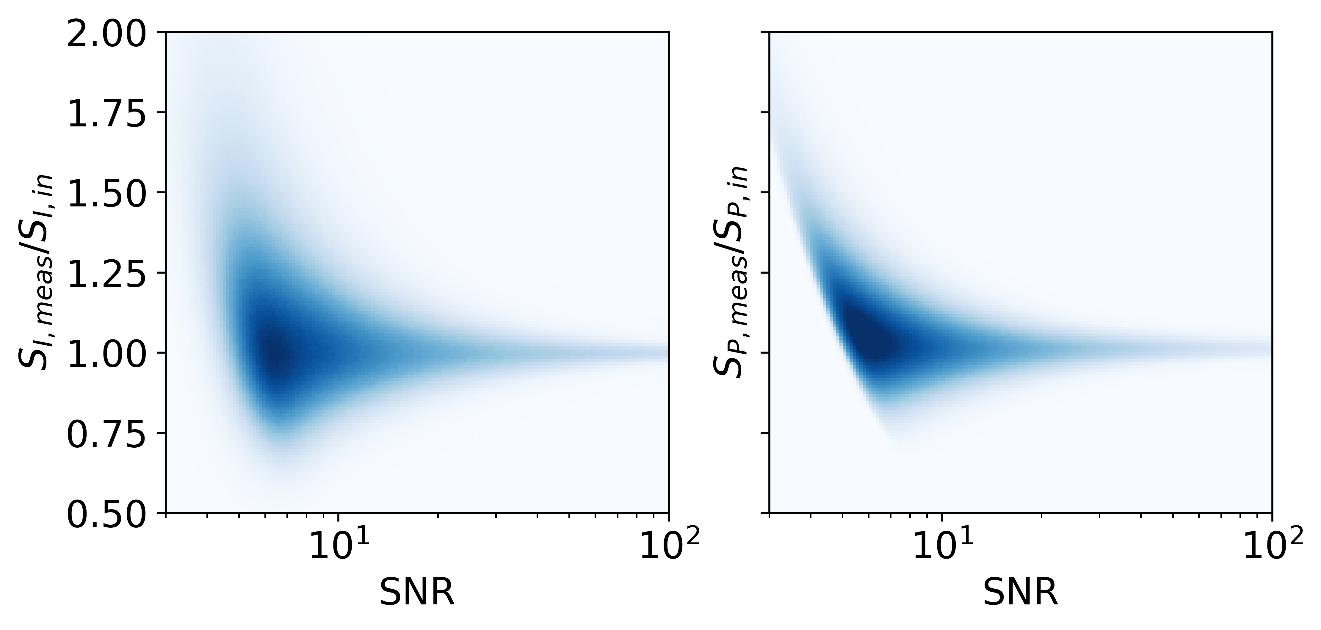
Figure 5: Comparison of the measured to input simulated flux density as a function of input SNR for the simulated sources in Shimwell et al. (2022) for both the integrated (left) and peak (right) flux densities.

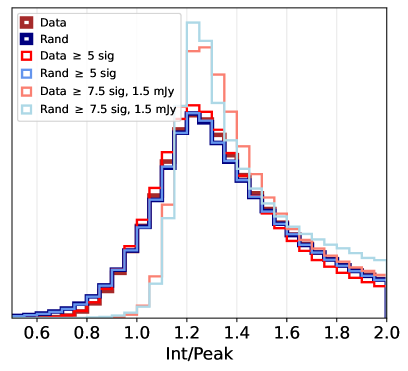
Figure 6: Normalised distribution of the integrated (Int) to peak flux density ratio for the data (blue) compared to the random sources (red). This is shown for all sources in LoTSS-DR2 and also those sources when a SNR cut of 5$\sigma$ is applied, and for the finally adopted cuts of 7.5$\sigma$, 1.5 mJy (see Sections 3.3.1 - 3.3.3). A lighter colour indicates a higher SNR cut.

We therefore resample our randoms to correct for the effects of:

1. The completeness as a function of both input SNR (peak flux density/rms) and integrated flux density;

2. The ratio of the input simulated peak flux density ($S_{\textrm{P, in}}$) to the measured peak flux density ($S_{\textrm{P, meas}}$) as a function of input SNR (to obtain a “measured" peak flux density);

3. The ratio of the input integrated-to-peak flux density ratio to the measured integrated-to-peak flux density ratio ($\frac{S_{\textrm{I, in}}S_{\textrm{P, meas}}}{S_{\textrm{I, meas}}S_{\textrm{P, in}}}$) as a function of input SNR (to obtain a “measured" integrated flux density).

We use the simulations of Shimwell et al. (2022) to take our input simulated catalogues and resample them to determine which sources are “detected” based on their expected completeness, given their SNR and integrated flux density. For those sources which were considered to be detected, we calculate a “measured” integrated and peak flux density for the simulated source.

To generate the final catalogue of randoms to be used to investigate the angular clustering we therefore take the input catalogue of random sources from SKADS discussed in Section 3.2.1 and calculate the peak flux densities that have been corrected for smearing (see Section 3.2.2). We also apply a further constant smearing ratio by dividing the peak flux densities by a ratio of 0.95; this was found to be essential to allow the peak of the integrated-to-peak flux ratio of the simulated sources to match that of the data, see Figure 6. The value was chosen to align the peak of these ratios and likely reflects a residual smearing issue from the data reduction processes such as from the effects of the ionosphere or residual calibration errors. Then, given the rms at the source location, it is possible to determine an input SNR.

Using this input source SNR and integrated flux density for an individual randoms source, we then calculate its completeness through interpolating from a 2D grid of completeness as a function of both SNR and flux density which have been calculated from the simulations of Shimwell et al. (2022), across all fields. For regions in SNR and flux density space where there is no or limited information from the simulations of Shimwell et al. (2022) to interpolate a completeness we extrapolate to reflect the detection. For example, at high SNR ($\geq 10$) and high flux densities where there is limited simulation information (and so can be affected by smaller number statistics), we assume all sources will be detected, and at low SNR ($\leq 1$), we assume the completeness is zero. From this 2D interpolation, we are able to calculate a probability associated with the completeness which is compared to a randomly chosen probability and is considered to be “detected” if the completeness value is larger than the random probability.

For these “detected” random sources, we then determine the “measured” peak and integrated flux densities for a source. This is important to consider because if we want to apply flux density or SNR cuts on the data (see Section 3.3) then such cuts would need to be applied to the random sources as well. Therefore, we again make use of the simulations of Shimwell et al. (2022) in order to generate a simulated “measured” peak and integrated flux density for each random source. To do this we again take the simulations from Shimwell et al. (2022) and construct a 2D histogram of the input SNR distribution vs. the ratio of the input to measured integrated flux density distribution (or similarly for peak flux density), for each pointing observed in LoTSS-DR2. To generate the measured flux densities, we use the input SNR of each random source and use random sampling to obtain a measured peak flux-density input-to-output ratio and to obtain a “measured” peak flux density. For the integrated flux density we sample to find the ratio between the input-to-output peak flux density to integrated source flux density ratio, given the source SNR. Again, we make sensible extrapolations in those regimes where we have fewer sources, for example at high SNR. Using this combined method means that we now have a distribution of random sources with not only positions, but also knowledge of the “measured” flux densities and SNR for the source.

3.2.4 Distribution of Randoms

This methodology leads to a distribution of randoms that can be seen in the lower panel of Figure 1. This, in general, matches that of the data (Figure 1) in that both under- and over-densities within the data are also apparent within the randoms in similar locations. This highlights that the process we are using to generate the randoms appears to broadly represent the observational biases across the field of view. However, as we believe there is real structure within the distribution of galaxies, there will be differences between the distribution of data and randoms across the image. There may, however, be additional SNR, flux density and positional cuts that need to be applied to the data to ensure the randoms reflect the data. We discuss such additional constraints in the next sub-section.

3.3 Additional Positional Constraints on the Data and Randoms

While these randoms have been generated across the full field of view of the LoTSS-DR2 survey, it is important to apply additional position-based constraints in order to account for known observational systematics within the data.

As discussed in Section 3.3.2 of Shimwell et al. (2022) and shown in their Figure 9, there appears to be variations in the flux scale across an individual pointing within the LOFAR field. This appears to be a result of differences in the model of the primary beam across the field of view. Such flux scale variations were seen to reduce by Shimwell et al. (2022) when pointings were mosaiced together. Therefore, we only include regions where pointings have been mosaiced together and by reducing the area of observations for both the data and the randoms to remove the outer edges. Furthermore, and for a similar reason, we want to remove those areas where there are a large number of gaps within the images due to facets that failed the data reduction process. These often, though not exclusively, lie towards the outer edges of the observations.

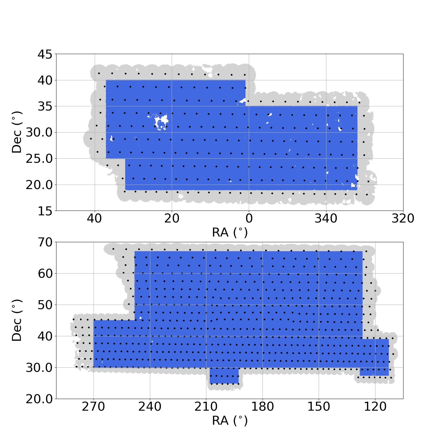
Figure 7: Distribution of sources in the 1h (top) and 13h (bottom) fields of LoTSS-DR2 for the full area (grey) and inner masked region (blue) that is presented in Table 1. The black dots indicate the pointing centres for each of the 841 fields observed. White regions indicate areas where the images are masked or outside the coverage of LoTSS-DR2.

The reduced area is defined in Table 1 and shown in Figure 7, alongside the locations of the centres of the 841 pointings which make up the DR2 region. The RA and Dec cuts are chosen to ensure that the data is at least a pointing radius from the outer edges of the observations. These cuts are employed to be conservative and remove regions where uncertainty may be introduced in the flux scale across the image as the region is not mosaiced with neighbouring pointings. With these cuts applied, we have $\sim$80% of the total area of LoTSS-DR2 remaining. This reduces the number of pointings which the data cover to 791.

Region	RA (∘)	Dec (∘)		Region	RA (∘)	Dec (∘)
1	[1, 37]	[25, 40]		5	[127, 248]	[30, 67]
2	[1, 32]	[19, 25]		6	[193, 208]	[25, 30]
3	[0, 1]	[19, 35]		7	[248, 270]	[30, 45]
4	[113, 127]	[27.5, 39]		8	[332, 360]	[19, 35]

Table 1: Definition of inner regions used to mask both the data and random catalogues as described in Section 3.3.

3.3.1 Validation of Randoms

In order to validate that our randoms are accurate before using them and to determine any additional cuts to apply in order to study the angular clustering, we first make comparisons to check that the data and randoms have similar distributions, using those within the region defined above (see Table 1). First, we consider the apparent completeness produced by the random catalogues and what this implies for the “intrinsic” source counts that would be estimated based on this completeness. We present the Euclidean normalised source counts distribution in Figure 8, where the raw data are compared to the “detected” random sources. As can be seen, there is good agreement between the raw source counts from the LoTSS-DR2 data and the “detected" randoms to a flux density of $\sim$0.3 mJy. Below 0.3 mJy, deviations likely arise from the fact that the minimum flux density used for the random catalogues was 0.1 mJy. Therefore, below $\sim 0.3-0.4$mJy it is likely that the corrections are mis-estimated as the full effects of detection biases (e.g. measurement and Eddington biases) in the flux densities for low SNR sources will not be probed fully. Further comparing the LoTSS random completeness corrected source counts to our input randoms sources, there are similar discrepancies below $\sim$0.3-0.4 mJy, which combines the resultant effects of not fully probing the correction for faint sources (as above) as well as the effect that the raw LOFAR data includes sources found from the wavelet fitting mode of PyBDSF, which is not modelled by the randoms. The effect of the wavelet fitting on the data can be better understood when we consider the SNR envelope of the data, which we discuss below.

We compare the SNR envelope of our data to that of the randoms catalogue in Figure 9. This presents the integrated to peak flux ratio as a function of detected SNR (measured peak flux density/rms). In theory, this would consist of sources with an integrated to peak flux density ratio of 1 if they are unresolved or a ratio greater than 1 if they are resolved. In reality, an envelope distribution is observed with increasing scatter in the ratio at low SNR. Figure 9 also shows there are a wealth of LoTSS-DR2 sources with SNR$<$5. These originate from PyBDSF’s wavelet fitting mode which was used during the source detection process. This is due to the fact that a new rms map is recalculated for each wavelet fitting scale. This mode is used for finding larger extended sources. However, the simulations from Shimwell et al. (2022) use smooth models for their simulated sources, so do not employ the wavelet fitting mode when source finding with PyBDSF. Therefore, a SNR cut of at least $5\sigma$ should be employed to ensure we use sources not detected through the wavelet fitting mode which have a different associated rms map that is not used here for the randoms. We present the comparison of the SNR envelope at $\geq 5\sigma$ for both the randoms and the data in Figure 9, which are in better agreement and for the final cuts to the data which are discussed in Section 3.3.1-3.3.3.

Both of the comparisons presented in Figures 8 and 9 examine the random populations as a whole, not as a distribution across the field of view and so we also consider the distribution of randoms and data across the field of view, within the inner regions bounded by the ranges listed in Table 1. In Figure 10 we present the distribution of the ratio of normalised number of data sources (normalising the number of sources in a bin to total number of sources) to the normalised number of randoms as a function of declination with various SNR and integrated flux density cuts applied. As can be seen, the comparison of data to randoms is shown both when the randoms are uniformly distributed across the sky as well as the randoms generated from the resampling process discussed in Section 3.2 above. An accurate distribution of randoms which reflect the underlying observational systematics should show a ratio which is close to, or scatters around, a value of 1.

Figure 10, demonstrates that up to a $5\,\mathrm{mJy}$ flux density limit, there is a clear difference between the uniform randoms and those which have the systematics of the data taken in to account. With just uniform randoms there is a clear declination dependence compared to the data, which likely reflects sensitivity variations across the sky. For example, the sensitivity becomes poorer at the lowest declination, therefore the uniform randoms will appear to be much more numerous than the sources observed in the data. However, the randoms generated for this work which account for sensitivity variations and observational systematics across the field of view show a more similar distribution to the data, oscillating around a value of 1. For higher flux density cuts, the comparison between the data and randoms becomes more similar to a ratio of 1, staying within $\sim$5% of a ratio of 1 above a flux density cut of 1 mJy.

Given the comparisons presented, it is clear that a 5$\sigma$ SNR (at least) is needed to avoid using those sources fit within the wavelet fitting mode of PyBDSF, whose rms maps will not reflect those used in this work. Furthermore, from the source counts distribution it has been discussed that at least a $0.3\,\mathrm{mJy}$ integrated flux density cut needs to be applied.

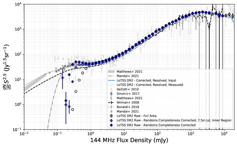
Figure 8: Euclidean normalised source counts for the input and recovered randoms compared to that from previous data and simulated models. The randoms that are used as an input model (pink, right facing triangles) and recovered (red, left facing triangles) are shown, both scaled to reflect the larger ratio of randoms to data. The raw LoTSS-DR2 counts are also shown (black open circles) as well as the corrected source counts from the completeness derived from the recovered randoms (navy crosses) and the corrected source counts from the raw counts across DR2 using the completeness from the simulations of Shimwell et al. (2022) both accounting for flux shifts between the simulated and detected flux density for a source (light blue dotted line) and not accounting for flux density shifts (blue solid line). Also shown is previous data from the LoTSS Deep Fields (Mandal et al., 2021, data - light grey stars and model - grey dot-dashed line) and source counts converted to 144 MHz from (Smolčić et al., 2017a, dark grey squares) and (Matthews et al., 2021, grey triangles). Also compared is the source counts model from the model of SKADS (Wilman et al., 2008, black dashed line) and modified SKADS model used in this work (black dotted line). Errors associated with source counts not presented in previous papers are determined using the relations from Gehrels (1986). When applying completeness corrections, we do not include uncertainty on the completeness as we only use a single randoms realisation. We also include the LOFAR corrected source counts using the raw data and completeness corrections from randoms when a 7.5$\sigma$ cut is applied over the inner region described in Table 1 (navy plus symbols, see Sections 3.3.1 - 3.3.3).

Figure 9: Distribution of integrated-to-peak flux density ratio (y-axis) as a function of measured SNR (x-axis) for the full LoTSS-DR2 survey (upper left), for the data with a 5$\sigma$ cut applied (upper centre) and for the randoms with a 5$\sigma$ cut applied (upper right) and with the 1.5 mJy and 7.5$\sigma$ final cuts applied (lower panels, see Sections 3.3.1 - 3.3.3).

3.3.2 Additional SNR and Flux Density Constraints

Despite the more advanced random catalogues presented in this work compared to Siewert et al. (2020) for the clustering of sources in LoTSS-DR1, we still may be limited by systematics in the data and may need to include additional cuts on the data and randoms. While Figure 10 has demonstrated that our randoms are smooth across the field of view as a function of declination, it cannot categorically show what flux density and SNR cuts to apply to the data and randoms in order to calculate the TPCF. We therefore consider the ratio across each pointing of the numbers of real sources to randoms (both normalised by the total numbers of real sources and randoms respectively) across the observations as a function of SNR and flux density cuts, specifically how the standard deviation in this ratio changes across each pointings. We use standard deviation, as opposed to the mean values as the mean values will fluctuate around a constant value, but it is the deviations in these which illustrate the variation of fields which appear to have an over- or under-density of randoms compared to data around a mean value. If there are observational effects which are unaccounted for in the generation of our randoms, these would cause larger standard deviations in the normalised ratios of data to randoms across the sky coverage.

In Figure 11 we present the variation of this ratio both across the full field of view (all 841 fields) and within the subset of pointings for which at least half of their sources lie within the inner region defined in Table 1 (where this limit is applied to avoid the effects of small number statistics). As can be seen, at a given SNR cut, the standard deviation declines with increasing flux density to $\sim 2\,\mathrm{mJy}$, where it begins to flatten. The right hand side of Figure 11 shows how the number of such sources in the data changes, given the cuts applied. As a compromise to balance both the number of sources we have as well as the variation in data compared to randoms, we apply a flux density limit of $1.5\,\mathrm{mJy}$ and SNR cut of 7.5$\sigma$ for this work. Referring back to Figure 10, it is clear that the distribution as a function of declination for such a SNR and flux density cut varies around a ratio of 1 within $\pm$5%. Hence we believe this will be sufficient and have a good reliability for our clustering measurements.

Therefore, we are still limited in this work to a similar high flux density cut (1.5 mJy) which is $\sim 15-20\times$ the typical point source sensitivity limit within the survey (70-100 $\muup$Jy), despite our additional investigations into generating accurate random sources. We believe that contributing to this may relate to residual field-to-field systematics across the field of view. Whether this relates to flux scale differences between pointings, as presented in Figure 9 of Shimwell et al. (2022), imperfect primary beam models or another residual observational systematic, remains unclear. Accounting for such residual systematics is something which is challenging to do within the simulations due to a lack of knowledge about, for example, these flux scale variations as a function of pointing. In order to assess any flux variations across the field of view, the LoTSS-DR2 sources would need to be compared with similar large area, deep radio surveys across the field of view, using a catalogue with known high flux density accuracy. However, such a similar large area, high-resolution and moderately deep survey which allows a relatively large number of sources at a similar frequency for flux density comparison across the full field of view is not available at present. For those large area surveys that are currently available, applying SNR cuts, isolation criteria and other cuts to ensure accurate comparisons of source flux densities between the two catalogues would lead to too few sources to accurately study the flux variations across each pointing. We therefore are reliant on applying flux density and SNR cuts until we can fully understand and account for additional remaining observational systematics.

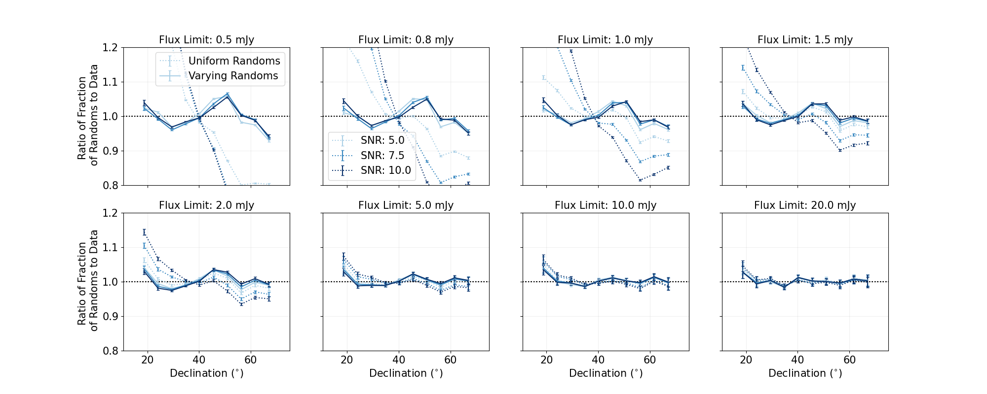
Figure 10: Comparisons of the ratio of the fraction of the total random sources to the fraction of the total data as a function of declination (accounting for differences in sample sizes) for the randoms generated using the methods in Section 3.2 (solid lines) and for randoms generated uniformly across the sky area (dotted lines) for sources $\geq$5$\sigma$ (light blue), 7.5$\sigma$ (blue) and 10$\sigma$ (dark blue) respectively in the regions defined by Table1. This is shown with increasing flux density cut applied when moving from top left to bottom right.

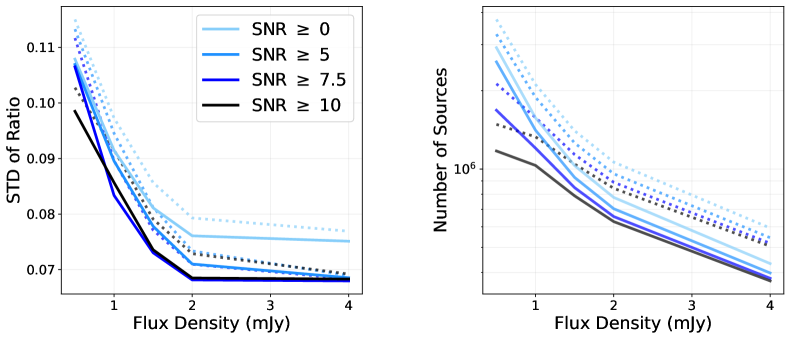
Figure 11: Standard deviations in the field-to-field scatter of the ratio of the LoTSS-DR2 sources to randoms across each individual pointings for different flux density and signal-to-noise cuts. Shown are the results for using the full field (dotted lines) and for those pointings which are within the inner region of Table 1 and contains at least 50% of the data sources in that pointing contained within the inner region (solid lines). The right hand figure uses the same colour scheme, but instead indicates the number of LoTSS-DR2 sources available for analysis.

3.3.3 Final data set

After applying the above SNR and flux density cuts as well as restricting to an inner region and also flagging three HealPix pixels (using $N_{\textrm{side}}$=256) which were contaminated by a nearby spiral galaxy (see Pashapour-Ahmadabadi et al. in prep), the number of sources which are used for these clustering studies is reduced. We present the number of data and random sources that are available after applying such cuts in Table 2. Such cuts help produce a random catalogue which we believe is accurate to measure the intrinsic large scale structure. The distribution of the final data and randoms used in this analysis can be seen in Figure 12.

Cut Applied	N${}_{\textrm{Data}}$	% of Initial Data Catalogue	N${}_{\textrm{Random}}$	% of Initial Random Catalogue	N${}_{\textrm{Randoms}}$/N${}_{\textrm{Data}}$
No Cuts	4,396,228	100	50,336,145	100	11.4
Inner Region	3,696,448	84	42,655,772	85	11.5
7.5$\sigma$ SNR cut	2,160,232	49	27,364,838	54	12.7
$1.5\,\mathrm{mJy}$ Flux Density cut	1,401,782	32	16,206,613	32	11.6
All cuts applied	903,442	21	11,378,354	23	12.6

Table 2: Number of data and random sources used when different cuts to the data are applied: using the inner region, a SNR cut and a flux density cut. The effects of these cuts on the data are presented individually as well as their combined effect on the catalogues (alongside the masking of 3 Healpix pixels, see text), in the bottom row. Presented are the number of data sources; the percentage of sources in the total catalogue that this consists of; the number of random sources; percentage of random sources compared to the initial (i.e. no cuts applied) random catalogue and the ratio of random sources to data sources with the same cuts applied.

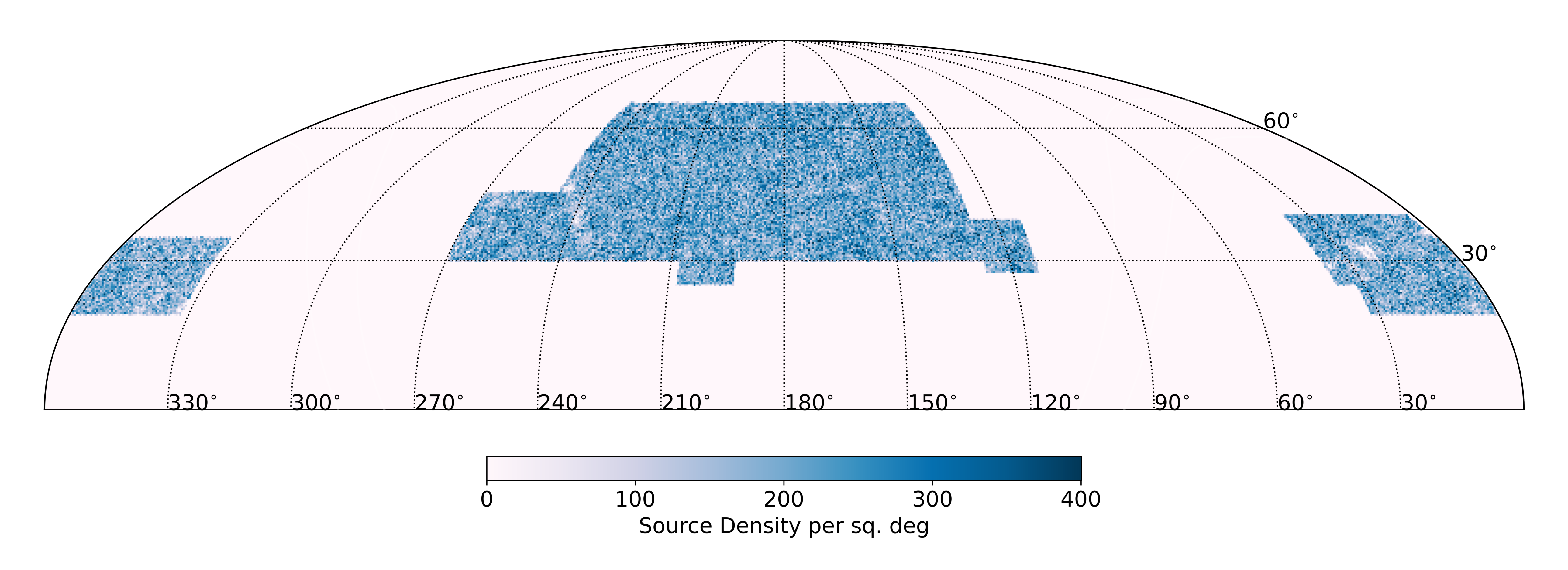
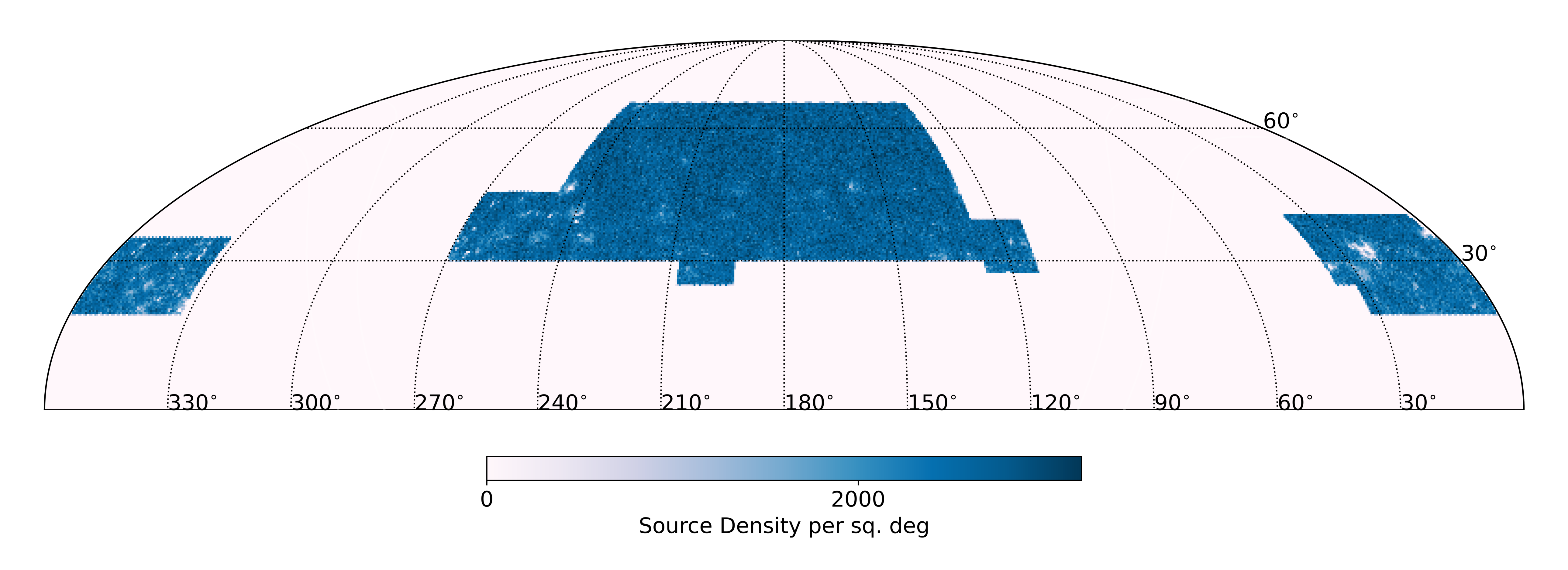
Figure 12: Sky distribution of data (upper) and randoms (lower) used in this work after cuts are applied to the data. These are plotted using Healpy in the mollweide projection. Note that the random sample is larger than the data sample, to minimise any Poisson errors associated with the randoms.

3.3.4 Changes in the process to create Randoms compared to LoTSS-DR1 and Remaining Limitations

As this paper follows on from the clustering studies within the first data release of the LoTSS survey (DR1) (see cosmology analysis presented in Siewert et al., 2020), we briefly summarise the developments in random catalogues generated in this work compared to in Siewert et al. (2020) as well as the additional cuts applied to the data. Firstly, in Siewert et al. (2020) the assumption was made that any sources above 5$\sigma$ are detected. However, as shown in the inset of Figure 4, at 5$\sigma$ the completeness is $\sim$50% on average. This work, instead, uses the completeness curves as a function of SNR from Shimwell et al. (2022) which take into account the varying completeness with SNR and, therefore, do not use a hard cut off. This will result in fewer sources in the 5-10$\sigma$ range (based on input signal-to-noise) being included within the random sample, though with a 7.5$\sigma$ cut (on measured signal-to-noise), this will reduce the impact of such effects. Secondly, we also take into account the source sizes and do not assume all sources are point sources. This aims to take into account the effects of resolution bias, which will affect completeness within our catalogue, though it does rely on a source shape model which has uncertainties in the true distribution. Observations at higher angular resolution, such as sub-arcsecond LOFAR surveys (see e.g. Sweijen et al., 2022), may aid with such knowledge but will be affected by resolution bias. Finally, we also calculate more accurately, for each random source, its “measured” peak and integrated flux densities. In Siewert et al. (2020) a flux density cut could be applied to the sources by ensuring the flux density added to the sampled noise associated with each source (which provides an estimate for a measured flux density) was greater than a given flux density limit. However, this used the same noise term which would be applied to the peak flux density. With this work, we are able to calculate the simulated to detected flux ratio as a function of SNR separately for the peak and integrated flux densities. This allows both SNR and flux density cuts to be applied on the appropriate “measured” flux density value.

While we have endeavoured to improve the generation of such random catalogues, residual caveats within the data still remain, which we discuss here for full clarity. Firstly, as discussed above, residual uncertainties in the beam model, flux density scale across the field of view and other un-accounted for observational biases may impact the accuracy of the random catalogues. We believe that these are a significant contribution to the inability to use fainter flux density/SNR cuts. While such flux offsets will average out when measuring e.g. source counts and declination dependencies over a full population, these will still exist on a field-to-field level. Furthermore, as we are not passing our randoms through a full end-to-end pipeline, there may be issues from the full LOFAR data reduction process, which we may not be fully able to account for the effects of. These include the effect of the ionosphere across each individual pointing, astrometric errors, the direction dependent calibration introduced by DDFacet or how individual fields are mosaiced together. The latter, especially, can lead to smearing of sources due to positional offsets within overlapping areas, which cover a large fraction of the observations. This smearing of sources may lead to a reduced sensitivity to detecting sources in the overlap regions and may affect the smearing model used at the largest distances from the pointing centre. These effects are challenging to model, as are the uncertainties in the intrinsic size distribution of radio sources. Whilst full end-to-end simulations (starting from simulating sources in the uv-data) could help such understanding, they are computationally expensive, especially for changes in the input source models considered.

With the methods discussed we have aimed to characterize as many of the systematics as possible in order to generate accurate random catalogues. While the effectiveness of the detailed analysis when creating random catalogues through mimicking observational biases is reduced by the effect of the larger flux density and SNR cuts adopted in this work, our presentation of a detailed discussion of the methods employed to generate the randoms as an example of methods which will be important for future analyses with deep radio surveys.

3.4 Errors on the TPCF

Once the randoms catalogues have been generated, it is possible to calculate $\omega(\theta)$ through Equation 5 and attribute uncertainties to our measurements. We consider several methods for quantifying the errors on the angular correlation function measurements. Possible errors include those from Poissonian statistics (i.e. just based on the number of sources observed within the data), bootstrap errors (where a random number of sources are replaced across the field of view) and jackknife errors (where regions are removed one area at a time and the scatter on the measured TPCFs assessed). Poissonian errors are known to underestimate the true errors (see e.g. Cress et al., 1996) and do not take in to account systematic variations in the data. For the naive estimate of $\omega(\theta)$ given in Equation 4, these Poissonian errors are given by:

$$\delta\omega_{\mathrm{Poisson}}(\theta)=\frac{1+\omega(\theta)}{\sqrt{DD(\theta)}}$$ (9)

However, when including the cross-terms ($DR$) in with the Landy-Szalay model, small changes to this are expected (see e.g. the equations presented in Landy & Szalay, 1993; Chen & Schwarz, 2016). Either way, such estimates of the errors do not account for potential systematics in the errors across the field. Therefore, we consider several methods which resample the data to assess the errors more accurately across the field of view. For bootstrap resampling, $\sim$1/3 of sources are randomly removed from the data and randomly replaced with the same number of randomly selected data sources. This means that a source from the original catalogue may not be in the bootstrap sample, be in it a single time, or multiple times. This process is then repeated in order to make $N_{B}$ resamples. For each resample, $\omega(\theta)$ is then calculated using TreeCorr as used for the original sample. The errors are then calculated from these as in Barrow et al. (1984); Ling et al. (1986):

$$\delta\omega_{B}(\theta)=\sqrt{\frac{1}{{N_{B}-1}}\sum_{i=1}^{N_{B}}[\omega_{i}(\theta)-\omega_{{B}}(\theta)]^{2}},$$ (10)

where $\omega_{B}$ is the mean value across the bootstrap samples. However, bootstrap resampling randomly removes sources and is not able to trace systematic trends across the data. If such systematics exist or if there is significant variation in source density across the field, it is therefore possible that bootstrap resampling underestimates the errors on $\omega(\theta)$.

We therefore, also consider using jackknife errors (see e.g. Norberg et al., 2009) which are calculated by splitting the field into a number of sub regions ($N_{J}$). One sub-region is then removed in turn and we measure the $\omega(\theta)$ from the remaining areas. The error is then calculated as:

$$\delta\omega_{J}(\theta)=\sqrt{\frac{N_{J}-1}{N_{J}}\sum_{i=1}^{N_{J}}[\omega_{i}(\theta)-\omega_{J}(\theta)]^{2}},$$ (11)

where $\omega_{{J}}$ is the mean value of the angular two-point correlation function across the samples where a sub-region has been removed.

For completeness, we present the errors measured for the TPCF for jackknife resampled errors, using TreeCorr to calculate the effect of changing the number of jackknife bins from 10 to 200. Finally, we consider the effect of field-to-field variations between the individual pointings of LoTSS-DR2. This method will directly probe the variations introduced from uncertainties between the different individual pointings of LoTSS-DR2. We calculate the errors from this using each pointing as a jackknife sample. We note that jackknife errors typically use regions of similar areas when calculating such errors, this will not be the case when calculating for the individual LoTSS-DR2 pointings being removed in turn. The internal pointings should be of roughly similar areas, but those towards the outside of the regions defined in Table 1 could be significantly smaller. However, such jackknife scales are more relevant to understand the variation across the field of view. A comparison of these resampling errors is presented in Figure 13, relative to the Poissonian errors. The relative sizes of the bootstrap and jackknife errors varies at different angular scales. At the smallest angles, $\theta\lesssim 0.1-0.2^{\circ}$, bootstrap errors appear larger. At larger angular scales the jackknife errors are, as expected, significantly larger than found from bootstrap errors. This likely reflects variations in the data across the field of view either due to real variation across the field of view or systematics within the survey across the field of view. The bootstrap errors are a factor of $\sim$2 larger than the Poissonian errors at angles $\lesssim$1^∘, increasing to a factor of $\sim$5 at 10^∘. In contrast, the jackknife errors are similar to within a factor of 2 to the Poissonian errors for $\theta\lesssim$0.2^∘, rapidly increasing to a factor of $\sim$10 larger at angles of $\sim$2^∘. In general, since our fitting of $\omega(\theta)$ will focus on the largest angular scales, our comparison suggests we should use jackknife errors, compared to bootstrap errors, in order to not underestimate uncertainties at large angular scales $\gtrsim 0.2$^∘. These larger angular scales are important for fitting linear bias, see Section 5.2.

The errors from jackknife resampling appear to be dependent on the number of jackknife samples considered, with larger errors for smaller samples and more comparable errors for $\gtrsim$50 resamples. The errors generated using the individual field-to-field variations are comparable to those calculated using Treecorr when 100-200 resampling bins are used, which is expected as $\sim$800 pointings are used for the field-to-field variations. As the field-to-field sizes are the most physically motivated binning as they are based off scales of the pointings within the LoTSS-DR2 samples, we present result using such errors. The covariance matrix for such errors is presented in Figure 14. We note that whilst the errors from TreeCorr compared to the field-to-field variation presented in Figure 13 appear similar for $N_{\textrm{Jack}}\geq 100$, the covariance matrix using TreeCorr has a larger contribution of off-diagonal covariance values, especially for small $N_{\textrm{Jack}}$. As such off diagonal covariance values can affect the fitting of the source, we therefore will also briefly discuss the effect on the measured bias values of instead assuming 100 jackknife bins as well, in Section 6.

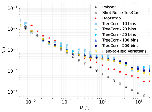
Figure 13: Comparison of the ratio of errors from different resampling methods. Shown are the naive Poissonian errors (black crosses, Equation 9), the shot noise errors measured for the sample using the Landy-Szalay estimator in TreeCorr (grey crosses), bootstrap errors (red stars) and Jackknife errors for 10 TreeCorr jackknife samples (light blue squares), 20 TreeCorr jackknife samples (light blue right triangles), 50 TreeCorr jackknife samples (blue diamonds), 100 TreeCorr jackknife samples (blue triangles) and 200 TreeCorr jackknife samples (navy circles) and field-to-field variation (yellow open crosses).

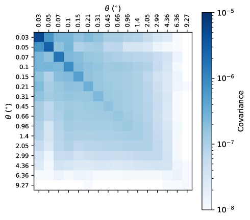
Figure 14: Covariance matrix from resampling the errors using a Jackknife approach where each individual observed LOFAR pointing (791 within the inner region) is removed in turn.

4 Angular Two-Point Correlation Function, $\omega(\theta)$

We present the angular two-point correlation function for LoTSS-DR2 sources with $S\geq 1.5\,\mathrm{mJy}$ and SNR$\geq$7.5 in Figure 15. This is shown above a minimum angular scale of $\sim$3$\times$ the PSF of the data ($\sim 3\times$6″ $\sim 18$″). As discussed in many previous studies (e.g. Peebles, 1975; Roche & Eales, 1999; Blake & Wall, 2002; Brodwin et al., 2008; Lindsay et al., 2014a; Hale et al., 2018), we can often describe the angular clustering at small angular scales ($\theta\ll\pi$) as a power law distribution, given by:

$$\omega(\theta)=A\theta^{1-\gamma},$$ (12)

where $A$ is the amplitude, $\theta$ is measured in degrees and the power law slope is given by $1-\gamma$. Observations suggest $\gamma$ has a typical value of $\sim$1.8 (see e.g. Peebles, 1975, 1980; Blake & Wall, 2002; Wilman et al., 2003), meaning that $\omega(\theta)$ follows a power law of slope -0.8.

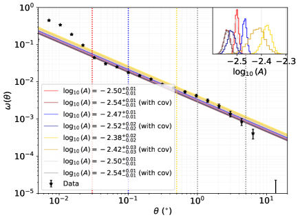
Figure 15: Angular TPCF, $\omega(\theta)$ for the final LoTSS-DR2 sample used in this work (black, see Section 3.3) from the range of $\theta:5\times 10^{-3}-10^{2}$^∘. Also shown if the fit to $\omega(\theta)$ of the form $A\theta^{-0.8}$ and the probability distribution in the value of $A$ is shown in the figure inset (top right). These are shown for fitting over the angular ranges: 0.03-5^∘ (red), 0.1-5^∘ (blue), 0.5-5^∘ (gold) as well as for the range where we reduce the largest fitting angle 0.03-1^∘ (grey) both without (light colours) and with (dark colours) the full covariance matrix, see Sections 4 and 5.2.

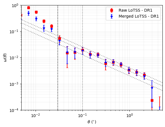
Figure 16: Comparison of $\omega(\theta)$ for LoTSS-DR1 Data (Shimwell et al., 2019; Siewert et al., 2020) for the raw PyBDSF catalogue compared to the source associated and cross-matched catalogue described in Williams et al. (2019) using a $1.5\,\mathrm{mJy}$ flux density cut and a $7.5\sigma$ SNR cut and presented with bootstrapped uncertainties.

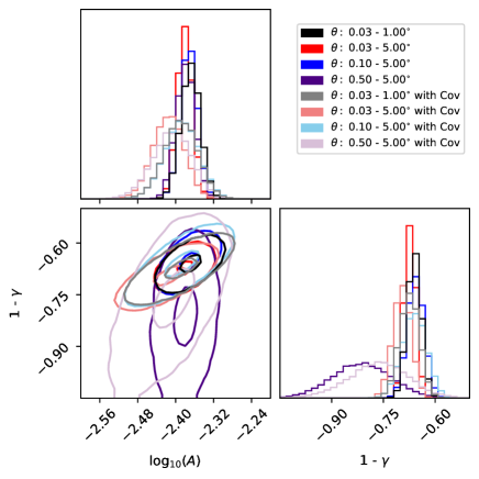
Figure 17: Angular TPCF fitting parameter constraints for both $A$ and $\gamma$ (with contours at 1 and 3$\sigma$) for fitting over the angular ranges: 0.03-5^∘ (red), 0.1-5^∘ (blue), 0.5-5^∘ (purple) as well as for the range where we reduce the largest fitting angle 0.03-1^∘ (black) both without (dark colours) and with (light colours) the full covariance matrix, see Sections 4 and 5.2.

As can be seen in Figure 15, our results for $\omega(\theta)$ appear to follow a power law with $\gamma=1.8$ over a large range of angular scales ($0.03\leq\theta<1^{\circ}$), at larger angles ($\theta\gtrsim{10}^{\circ}$) there is more uncertainty on the value of $\omega(\theta)$ and so we do not present such scales in this work. At small angles ($\theta\lesssim 0.03^{\circ}$), there is a deviation from this power law distribution. This could arise from a combination of factors: (a) clustering of galaxies within the same dark matter halo and (b) the effect of multi-component sources.

The first of these contributions to the excess clustering at small angular scales is related to whether the clustering of galaxies we are observing is from sources that are residing within the same dark matter halo (this is observed at small angular scales and is known as the ‘1-halo’ clustering, see e.g. Zehavi et al., 2004). Measurements of the ‘1-halo’ clustering require observations which are both sensitive enough to observe multiple galaxies within the same dark matter halo and also have the resolution to ensure any galaxies within the same dark matter halo are not confused into a single source. In the radio, this ‘1-halo’ clustering has been challenging to observe due to the depths and resolutions of surveys previously observed, however it will become increasingly possible with future deep, high-resolution radio surveys. When discussing clustering previously, we have instead focused on the clustering from galaxies in different dark matter haloes (known as the ‘2-halo’ clustering) which presents as the power law behaviour given in Equation 12 on large angular scales).

The second contribution to the excess clustering at small angular scales, on the other hand, relates to the source detection within radio catalogues. For example, a jetted radio galaxy could be observed to have a core and two lobes separated from it. Depending on the separation of these lobes, conventional source finders (e.g. Whiting & Humphreys, 2012; Mohan & Rafferty, 2015; Hancock et al., 2018) may not be able to accurately characterise the components of the radio galaxy into a single source. As such, accurate cross matching of radio components relies on techniques such as visual identification (see e.g. Banfield et al., 2015; Williams et al., 2019), or machine learning/algorithm based techniques (see e.g. Galvin et al., 2020; Barkus et al., 2022; Alegre et al., 2022). If, in this example, the three components of the single radio source are catalogued to be different objects, then this will result in seeing an apparent excess angular clustering at small angular scales (see e.g. Blake & Wall, 2002; Overzier et al., 2003), which can be described as a power law with a steeper slope. To determine the angular scales below which such multi-component sources may become important in our work we consider the clustering in LoTSS-DR1 with both the raw PyBDSF catalogue and the value added catalogue of Williams et al. (2019), where PyBDSF source components were combined into physical sources. We use the randoms generated for Siewert et al. (2020) and apply a 1.5 mJy and 7.5$\sigma$ cut, as used in this work, and present the clustering with and without source associations in Figure 16. This demonstrates a deviation between the raw and merged (source associated) catalogues, for which a deviation is seen at angles below 0.03^∘. This therefore suggests that the impact of multi-component sources is likely important below such an angular threshold and so we should not fit our $\omega(\theta)$ for LoTSS-DR2 below this scale.

We fit $\omega(\theta)$ using Equation 12, with a maximum angular separation of 5^∘ and a minimum angular separation of either (i) 0.03^∘, below which multi-component source clustering becomes important; (ii) 0.5^∘ below which models that include both 1- and 2-halo clustering can diverge (see Section 5.2 for fitting with the cosmology code CCL, Chisari et al., 2019) and (iii) 0.1^∘  as a compromise between the two angular fitting ranges. Finally, we also include an angular fitting range of $0.03\leq\theta<1$^∘to reflect the fact that the approximation of a power law model for $\omega(\theta)$ breaks down at large angles. In our model we also include an extra term known as the integral constraint which accounts for finite field sizes (see e.g. Roche & Eales, 1999). We therefore calculate the $\chi^{2}$ through the difference between the observed data and the model (with the integral constraint subtracted), using two methods. The first method, that we adopt, solely accounts for the diagonal elements of the errors ($\delta\omega$, as compared in Figure 13), defining $\chi^{2}$ as:

$$\chi^{2}=\sum_{i=1}^{N_{\theta}}\left(\frac{\omega(\theta_{i})-\omega_{M}(\theta_{i})}{\delta\omega_{i}}\right)^{2},$$ (13)

where $\omega_{M}(\theta_{i})$ is the model for the angular clustering, as in Equation 12, for a given angular bin ($\theta_{i}$) and is fit across the $N_{\theta}$ bin in the angular range considered. This does not encapsulate the full systematic correlations between $\theta$ bins, but allows for a comparison to previous works who use such methods for fitting $\omega(\theta)$. The second method uses the full covariance matrix, which allows correlations between $\theta$ bins to be accounted for. For this method, we calculate $\chi^{2}$ as:

$$\chi^{2}=(\vec{\omega}-\vec{\omega}_{M})^{T}{\rm Cov}^{-1}(\vec{\omega}-\vec{\omega}_{M})$$ (14)

where Cov is the associated covariance matrix for our measurements of $\omega(\theta)$, as calculated by TreeCorr. The $T$ indicates that the transpose is being used. We fit a model for $\omega(\theta)$ using both Equations 13 and 14 to highlight the differences of accounting for the full covariance.

When fitting solely for $A$ (and fixing $\gamma$ to 1.8), we measure the variation in $\chi^{2}$ when fitting the data using values of $\log_{10}(A)$ which are uniformly sampled from $-4$ to $-2$. From the $\chi^{2}$ distribution we calculate a probability distribution ($P\propto{\rm e}^{-{\chi^{2}/2}}$) and use a resampling method with 5000 samples to calculate a median value and associated error bars from this sample. The results are presented in Table 3 and Figure 15. As can be seen in Figure 15, the chosen angular scale below which we do not fit the data, $\theta<0.03^{\circ}$, appears to be an appropriate scale to restrict the fitting over. Below these angular scales we observe a significant increase in $\omega(\theta)$, which we attribute to the contribution of the combination of multi-component sources and 1-halo clustering. Figure 15 shows the best fit models to the clustering amplitude, $\textrm{log}_{10}A$, of -2.50$\pm$0.01 (using $\chi^{2}$ as in Equation 13) and -2.54$\pm$0.01 (using the full covariance) when fit over the largest angular range (0.03-5^∘). When fitting to the lower maximum angular scale ($0.03\leq\theta<1$^∘) we find little difference to that when fitting in the range $0.03\leq\theta<5$^∘. Whilst fitting $\omega(\theta)$ using Equation 13 shows a good fit to the data on a large range of angular scales, there is a deviation from such a power law around 1^∘. This results in an increased clustering amplitude when fitting across the largest angular scales only 0.5-5^∘, which then over-estimates clustering on smaller scales. This may suggest some excess residual systematics in the data, on the scale of $\sim 1^{\circ}$. The fits using Equation 14 also appear to underestimate the values for $\omega(\theta)$ to more of an extent than with Equation 13.

To test whether the assumed slope of -0.8 is suitable for this work, we also fit $\omega(\theta)$ for both $A$ and $1-\gamma$, using a fitting range of $-4$ to $-1$, for $\log_{10}(A)$ and $-2$ to $0$ for $1-\gamma$. We fit this using the Markov Chain Monte Carlo (MCMC) code, emcee (Foreman-Mackey et al., 2013). We fit using 100 walkers, each with 5000 chain steps and remove the first 90% of chains as burn in. From this, we fit for $A$ and $\gamma$ using likelihoods based on the $\chi^{2}$ described in Equations 13 and 14. The results for such fitting across the angular ranges described above are presented in Figure 17 which, for the majority of angular scales, find a value of $1-\gamma\sim-0.6$ to $-0.75$, shallower than the $-0.8$ slope assumed when fixing $1-\gamma$. However, previous measurements of $1-\gamma$ using radio surveys (see e.g. Magliocchetti et al., 2017; Lindsay et al., 2014a, b) have found that such slopes ($1-\gamma$) observed for radio surveys are typically closer to $-1.2$ to $-0.8$. The differences observed here may therefore relate to a combination of factors, such as residual systematics in the data (as discussed above and in Section 3.3.4) as well as effects of combining multiple source populations in our measurement of $\omega(\theta)$. As such, we will predominately use our measurements where we fix the slope of $\gamma$ in order to measure bias, though in Section 5 and 6 we will discuss the effect on the bias of assuming a variable slope.

4.1 Variation with Location and Flux Density

In order to investigate the uniformity of $\omega(\theta)$ given the possibility of systematics we are unable to correct for, we also present comparisons of the angular clustering of the LoTSS-DR2 data as a function of Right Ascension, Declination and position within the full field of view. To do this, we consider the TPCF in RA angular ranges spanning 40^∘ and declination in angular ranges spanning 10^∘  and finally within nine different regions spread across the field of view in RA and Dec bins as presented in Figure 18. Uniform RA and Dec ranges are used to generate the RA and Dec bins, this will lead to significant differences in the number of sources in each of the bins which will have a more substantial impact on the measured $\omega(\theta)$ in regions where there are fewer sources. This analysis, follows on from the comparisons of Siewert et al. (2020), in which three regions were used to consider the variation in the angular clustering of LoTSS-DR1.

The resulting variations in $\omega(\theta)$ are presented in Figure 19. As can be seen, the variation of the angular clustering is typically restricted to larger angles $\theta\gtrsim 0.5^{\circ}$, whilst smaller angles are typically in much better agreement with one another. Whilst there are no apparent trends with RA, there may be a suggestion of a systematic trend in the angular clustering observed with declination, with higher observed angular clustering at typically lower declinations. However, this is not seen at all angular scales. We also see there is more variation in the measured $\omega(\theta)$ when split into RA ranges and the regions presented in Figure 18. As discussed in Sections 3.3.2 and 3.3.4, we believe there are still limitations in the data which the randoms do not account for, such as individual flux shifts between pointings, uncertainty in the beam models and remaining systematics not modelled as full end-to-end simulations were not used to generate the random sources. It is possible that the effect of these can be a cause of the variation of $\omega(\theta)$ when split by these sky regions however, true underlying large scale structure may also play a role. The spread with declination is much smaller, with $\omega(\theta)$ in the Dec: 60-70^∘ bin showing the most variation, likely due to the smaller area and number of sources in this region. This smaller variation is likely due to the corrections implemented for elevation dependent smearing, which is related to the declination for fields observed with a good hour angle coverage. If there are residual systematics relating to flux shifts between pointings (as described in Shimwell et al., 2022), these are challenging to identify and model using available radio surveys. These effects and a combination of other residual systematics may relate to why there can be variations between $\omega(\theta)$ in different regions of the data. Identifying the cause of these and making further corrections may be possible in the future, with further understanding of the systematics.

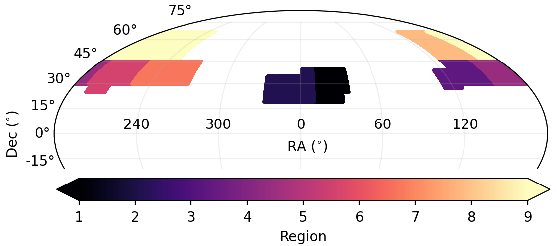
Figure 18: Regions used to investigate the TPCF variation as presented in Figure 19. Each colour indicates a different region used to quantify the TPCF.

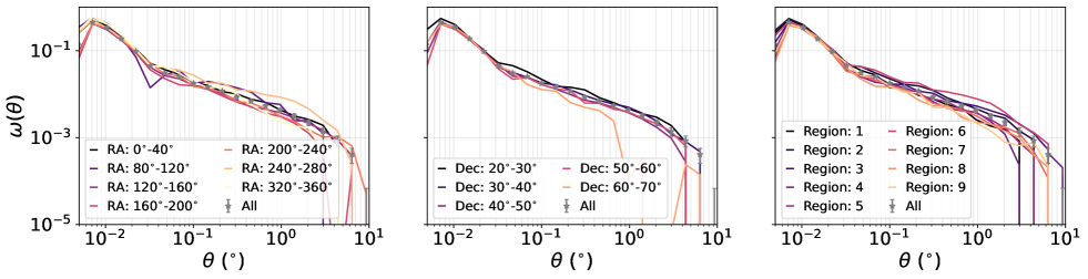
Figure 19: The clustering variation between regions which are split based on their right ascension (left), declination (centre) and their location within the DR2 region as presented in Figure 18 (right). The colour of the lines present the RA range, Dec range or region being considered and the results of the full area of the survey are shown in grey (stars). Only the $\omega(\theta)$ value is presented for each subset, not the associated errors.

5 Galaxy Bias

Whilst fitting a clustering amplitude, $A$, allows for a comparison with previous work, it is also challenging to compare with previous studies due to its dependence on flux density, luminosity and source type within the same sample (see e.g. Wilman et al., 2003; Overzier et al., 2003; Magliocchetti et al., 2017; Hale et al., 2018; Chakraborty et al., 2020). We calculate the more physical parameter of bias, $b(z)$. As discussed in Section 1, bias traces the clustering compared to matter and can be used to estimate the typical dark matter halo mass hosting a population of sources (see e.g. Berlind & Weinberg, 2002; Zehavi et al., 2004). By calculating the bias, we not only calculate a more physical parameter, but also account for the redshift distribution of the sources being investigated. However, this will also have a dependence on flux density, as the relative contribution of different source types to the overall population (e.g. AGN, SFGs) varies with flux density (see Best et al., 2023, for a comparison of this in the LoTSS Deep Fields). These populations can have different bias values and so will affect the bias measured for a full population (see e.g. Magliocchetti et al., 2017; Hale et al., 2018; Chakraborty et al., 2020).

In order to obtain measurements of the bias for the LoTSS-DR2 sources, knowledge of the redshift distribution, $p(z)$, for the data is required. This is because $\omega(\theta)$ is a projected measurement of the clustering of galaxies over the sky, and to understand the bias, we need to understand the true spatial distribution. Using a given $p(z)$ we then take two approaches to modelling the clustering: (1) fitting using the cosmology code, CCL (Chisari et al., 2019) and (2) using the power law model fit for the amplitude, described in Section 4, and using Limber’s inversion (see Limber, 1953, 1954; Peebles, 1980, assuming a power law model for $\omega(\theta)$ to calculate a clustering length, $r_{0}$, and subsequently a measurement of the bias), as has been commonly employed in clustering studies for radio surveys (see e.g. Magliocchetti et al., 2004; Lindsay et al., 2014a; Magliocchetti et al., 2017; Hale et al., 2018; Chakraborty et al., 2020; Mazumder et al., 2022). We will describe both approaches, below, however we first describe how the redshift distribution, $p(z)$, for the data is obtained, as this is critical for both approaches.

5.1 Redshift distribution

In order to calculate the bias, we must assume a redshift distribution for the sources in our sample, which is not possible from radio continuum measurements alone. Instead, a catalogue where radio data and multi-wavelength data have been cross-matched together (as with LoTSS-DR1, see Williams et al., 2019; Duncan et al., 2019), may provide redshifts for some sources however, redshifts are not currently available for a relatively complete population of LoTSS-DR2 sources. Therefore, in order to estimate the expected redshift distribution of the sources observed in LoTSS-DR2, we make use of the LoTSS Deep Fields observations (Tasse et al., 2021; Sabater et al., 2021; Kondapally et al., 2021; Duncan et al., 2021). The LoTSS Deep Fields data are more sensitive than in LoTSS-DR2 (reaching an rms $\sim 20-40\,\muup\mathrm{Jy}\,\mathrm{beam}^{-1}$) over three extragalactic fields (see Section 2.2 for details). For the Deep Fields sources, 97% have been cross-matched to a multi-wavelength host galaxy (Kondapally et al., 2021) and have an associated redshift (Duncan et al., 2021). A full probability distribution for the photometric redshift, $p_{i}(z)$, of those sources with an associated host galaxy is presented in Duncan et al. (2021), which we use in this work.

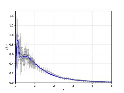
Figure 20: Weighted redshift distribution generated from combining redshift distributions in the LoTSS deep fields (grey) as described in Section 5.1. The distribution of models fit to the resampled $p(z)$ as described in Section 5 are presented as the median in blue (solid line) alongside the 16${}^{\textrm{th}}$ and 84${}^{\textrm{th}}$ percentiles respectively (as dashed lines).

To determine the redshift distribution for the sources observed here, we first apply a $1.5\,\mathrm{mJy}$ flux density cut to the cross-matched radio deep-field catalogues, matching that used here for LoTSS-DR2. Specifically, we take an individual field and generate $N_{f}$ estimates for the redshift distribution, where $N_{f}$ across the three fields totals 1000 samples. The $N_{f}$ values are weighted for each field to gives more samples where there are larger number of $S\geq 1.5$ mJy sources in the field. To make a single resample within a field, we use those sources which have $S\geq 1.5$ mJy and generate a resampled redshift for those sources through the following process. For those sources with a photometric redshift, we sample from the full $p_{i}(z)$ distribution for the individual source. For those sources where a spectroscopic redshift exists, we instead consistently use the spectroscopic value. From the resampled redshifts for the $S\geq 1.5$ mJy sources, we create a $p(z)$ by binning the redshifts and normalising the resultant distribution. When binning the redshift distribution, we use bins which have more frequent binning at low redshifts ($z\leq 1$, using $\delta z=0.02$, where we have more accurate spectroscopic information) and coarser binning at higher redshifts ($z>1$ , using $\delta z=0.1$). To generate the redshift distribution across the fields, we combine the samples from each field to produce 1000 resampled $p(z)$ distributions. From this we are able to determine a mean $p(z)$ distribution and associated errors from the standard deviations of the sample. The final $p(z)$ and errors is presented in Figure 20.

To use this $p(z)$ in our fitting and modelling of $b(z)$, we generate 1000 resampled $p(z)$ distributions using the mean and standard deviation across each redshift bin. We do this, as opposed to using the 1000 samples combined from the three fields, to avoid extreme models in each field that are driven by cosmic variance affecting such measurements, as well as the effects of multi-wavelength data availability. In order to ensure that such randomly sampled values does not lead to a highly varying $p(z)$ and satisfies $P(0)=0$. We model the resampled redshift distribution using a functional form given by:

$$p(z)\propto\frac{z^{2}}{1+z}\left[\exp\left(-\frac{z}{z_{0}}\right)+\frac{r^{2}}{(1+z)^{a}}\right],$$ (15)

which we normalise such that it becomes a probability density function.

Such a functional form is found to appropriately represent the redshift distribution, and was chosen to allow contributions from AGN and SFGs to the full redshift distribution. The form reflects the probed volume of a $\Lambda$CDM model at small redshifts with the exponential and power law terms representing the high luminosity cut-offs at large redshifts of SFGs and AGNs respectively (for more description see Nakoneczny et al. in prep). The model parameters ($z_{0}$, $r$ and $a$) are fit for each resample using scipy’s curve_fit function. The range of the modelled redshift distribution from these resamples are presented in Figure 20.

We note that with this method, the $\sim$5% of LoTSS Deep Fields sources above $1.5\,\mathrm{mJy}$ which have no associated redshift distribution cannot be included in $p(z)$. This may bias the results slightly, likely by missing some very high redshift AGN or SFGs and those which are dust obscured. Furthermore, there are potential biases in the $p(z)$ due to the band selection and magnitude limits of the multi-wavelength data. For example, sources may not be detectable in all bands and there is differing availability of multi-wavelength data in the three deep fields, both of which will affect constraints which can be placed on their redshift distributions. Moreover, the deep fields are much smaller areas than the full LoTSS-DR2 survey, and so are more likely to be affected by variances in large-scale structures, however we mitigate this by averaging across the three fields. Finally, it is challenging to apply similar SNR cuts to the deeper LoTSS Deep Fields data, which may lead to residual systematics in the $p(z)$ models. However, this combined $p(z)$ is the best model available for a representative radio population and those sources without any redshift information only represent a very small fraction of sources in the data.

5.2 Measuring $b(z)$ using CCL

In the first method to determine $b(z)$, we use CCL to fit $\omega(\theta)$, assuming a bias model. For this work we follow the work of Alonso et al. (2021) and assume two possible bias models either (i) a constant bias i.e. $b(z)=b_{0}$ or (ii) an evolving bias of the form $b_{0}$/$D(z)$, where $D(z)$ here is the normalised (to $z=0$) growth factor as described in e.g. Hamilton (2001). We also consider two matter power spectrum models (i) a ‘linear’ model where only linear perturbation theory was assumed and (ii) a ‘HaloFit’ (Smith et al., 2003; Takahashi et al., 2012) model where non-linear effects within a dark matter halo are also accounted for. Both models are considered as we may not expect to observe a strong contribution from ‘1-halo’ clustering at the depth of this survey, or that if such 1-halo contribution does exist that this may dominate predominately in the angular region where effects of multi-component sources is also important (see Figure 16). We use the $\ell$ range $1\leq\ell\leq 10,000$ in 256 logarithmically spaced bins to generate the $C_{\ell}$ power spectrum with CCL and then use this to determine $\omega(\theta)$ over the $\theta$ range used in this work using a Legendre polynomial transform given by:

$$\omega(\theta)=\frac{1}{4\pi}\sum_{{\ell}}(2\ell+1)C_{{\ell}}P_{{\ell}}(\cos\theta).$$ (16)

Such a conversion from $C_{{\ell}}$ to $\omega(\theta)$ was also used in Siewert et al. (2020). To obtain $C_{{\ell}}$, we use the conversions in CCL which convert the 3D power spectrum to $C_{{\ell}}$ using the equations in Section 2.4.1 of Chisari et al. (2019), but assuming the redshift space distortion and magnification bias terms can be neglected:

$${C_{\ell}=\int\frac{d\chi}{\chi^{2}}\,q^{2}(\chi)\,P\left(k=\frac{\ell+1/2}{\chi},z(\chi)\right),}$$ (17)

where $\chi$ is the comoving radial distance, $P(k,z)$ is the matter power spectrum, and the radial kernel $q(\chi)$ is:

$${q(\chi)=\frac{H(z)}{c}\,b(z)\,p(z),}$$ (18)

with $H(z)$ the Hubble parameter. This relation relies on Limber’s approximation (Limber, 1953, 1954), which is valid for the broad redshift distribution explored here.

We fit for $b_{0}$ through calculating $\omega(\theta)$ with CCL and fitting to the data using Equations 13 and 14. Again, when fitting the data we consider three angular ranges: $0.03^{\circ}-5^{\circ}$, $0.1^{\circ}-5^{\circ}$ and $0.5^{\circ}-5^{\circ}$. We also consider all possible combinations of linear and HaloFit models with the two bias evolutionary models. To determine $b_{0}$ we use the 1000 redshift resamples described in Section 5.1. Firstly, we calculate $\omega(\theta)$ for each resampled redshift distribution, assuming $b_{0}=1$ (denoted here as $\omega_{b_{0}=1}(\theta)$). Using this, we select random bias values within the range 0.5-3.5 and generate a model $\omega(\theta)$ through multiplying $\omega_{b_{0}=1}(\theta)$ by $b^{2}$. Using such a predicted model and comparing to the data we then calculate the associated $\chi^{2}$ across the angular fitting ranges described above and calculate this both assuming only diagonal elements as well as using the full covariance matrix. The full covariance will highlight if there are correlations in the $\omega(\theta)$ values at different $\theta$ which can affect the fitting of $b$. In both cases we take the “model” to be the model produced from CCL with the integral constraint as modelled in Roche & Eales (1999), though the contribution of an integral constraint will be negligible. Using such a $\chi^{2}$ value we then calculate an associated probability for $b_{0}$ assuming $P(b_{0})\propto e^{-\chi^{2}/2}$ (which makes the assumption that errors on the data can be approximated as Gaussian).

To determine final values of $b_{0}$ found from fitting our observations we then resample from $P(b)$. To do this, we consider two possibilities of how to include the redshift distribution to determine $b_{0}$. The first case assumes that the individual redshift resamples described in Section 5.1 are all equally probable. In this case, any differences which may remain between the model and observations will reflect residual systematics in the data which are unaccounted for in the random catalogues or that a different bias evolution model is appropriate. For this method, we renormalise the $P(b)$ model from each redshift sample to 1. The second case assumes that there are no remaining systematics and so redshift resamples which better fit the data reflect the intrinsic $p(z)$ of our sample can be determined. In this case we do not normalise $P(b)$ for each sample to 1 before resampling and instead retain the difference in probabilities based on the magnitude of the $\chi^{2}$.

Through resampling the data we determine $b_{0}$ accounting for the uncertainty in $p(z)$ models. In the first method, this means that the contribution of $p(z)$ samples from those models which satisfy the resampling criteria are approximately evenly distributed across the 1000 redshift resamples and, as such, some $p(z)$ samples may lead to large $\chi^{2}$ values where the magnitude of the $\chi^{2}$ for such a $p(z)$ was large. In the second method, there will instead be preferred $p(z)$ samples and others may not have any (or very little) contribution to the bias values which satisfy the resampling criteria, whilst other $p(z)$ models may substantially dominate the sample. This can lead to only a small fraction of $p(z)$ samples actually contributing to the fit, especially when the fit is poor. Due to this method, the associated $\chi^{2}$ values of the fit will be lower to that of the previous method. The $b_{0}$ values these are quoted as the median value with errors measured from the 16th and 84th percentiles and are presented in Table 4 and Figure 22. To present associated models of $\omega(\theta)$ we use 10000 realisations of the final $b_{0}$ sample to determine $\omega(\theta)$ models, this is shown in Figure 21 for the evolving and constant bias models.

5.3 Fitting $b(z)$ using Limber’s equation for a power law model of $\omega(\theta)$

The second commonly used method to infer the spatial clustering of galaxies from the angular clustering is by using Limber’s equations after assuming a power law model for $\omega(\theta)$ (see e.g. Limber, 1953, 1954; Peebles, 1980). This method has been frequently employed in studies of the clustering of galaxies both at radio frequencies (see e.g. Lindsay et al., 2014a; Hale et al., 2018; Chakraborty et al., 2020; Mazumder et al., 2022) and other frequencies (see e.g. Puccetti et al., 2006; Starikova et al., 2012; Cochrane et al., 2017). To quantify $b(z)$, we use the fitting of $\omega(\theta)$ as described in Equation 12, discussed in Section 4, with the parameterisation of the spatial clustering:

$$\xi_{g}(r)=\left(\frac{r}{r_{0}(z)}\right)^{-\gamma}=\left(\frac{r}{r_{0}}\right)^{-\gamma}(1+z)^{\gamma-(3+\epsilon)},$$ (19)

where $r_{0}$ is a spatial clustering length which parameterises the clustering of galaxies and $\epsilon$ describes the evolving clustering model. $\xi_{g}(r)$ is the spatial clustering of galaxies, as introduced in Section 1. We present $r_{0}$ and $b$ measurements using two assumptions for $\epsilon$: (i) assuming ‘comoving’ clustering, where $\epsilon=\gamma-3$, to make comparisons with previous studies (e.g Lindsay et al., 2014a, b; Hale et al., 2018; Mazumder et al., 2022) and (ii) assuming ‘linear’ clustering, where $\epsilon=\gamma-1$, which probes a different range of bias evolution, see Lindsay et al. (2014a). In order to determine the spatial clustering, we need both knowledge of $\gamma$ and $A$ from Equation 12 as well as $p(z)$ to determine the spatial clustering length, $r_{0}$. As discussed, in the majority of cases we fix $\gamma$ to a value of 1.8, though we also consider the case for a variable $\gamma$ for comparison. The value of $r_{0}$, can then be calculated using Limber’s equation (see e.g. Limber, 1953, 1954; Peebles, 1980):

$$r_{0}=\left(\frac{A_{\textrm{r}}\ c\ \left(\int_{0}^{\infty}p(z)dz\right)^{2}}{H_{\gamma}H_{0}\int_{0}^{\infty}E(z)^{\frac{1}{2}}p(z)^{2}\chi(z)^{1-\gamma}(1+z)^{\gamma-(3+\epsilon)}dz}\right)^{\frac{1}{\gamma}},$$ (20)

where $c$ is the speed of light in km s^-1, $E(z)=\Omega_{m}(1+z)^{3}+(1-\Omega_{m})$ and $\chi(z)$ is the comoving distance at redshift, $z$. $A_{r}$ is related to the amplitude ($A$) in Equation 12 when $\theta$ is in the unit of radians. Finally, $H_{\gamma}$ is given by:

$$H_{\gamma}=\frac{\Gamma(\frac{1}{2})\Gamma(\frac{\gamma-1}{2})}{\Gamma(\frac{\gamma}{2})},$$ (21)

where $\Gamma$ represents the gamma function. As described in Section 1 and Equation 2, the spatial clustering of galaxies can be related to that of matter to parameterise galaxy bias. Following analysis from Peebles (1980) and discussed and used in works such as Koutoulidis et al. (2013); Lindsay et al. (2014a); Hale et al. (2018); Mazumder et al. (2022), the bias can then be inferred from $r_{0}$ using:

$$b(z)=\left(\frac{r_{0}(z)}{8\textrm{Mpc}h^{-1}}\right)^{\gamma/2}\frac{J_{2}^{1/2}}{\sigma_{8}D(z)/D(0)},$$ (22)

where $D(z)$ is the growth factor, and $J_{2}$ is given by $\frac{72}{2^{\gamma}(3-\gamma)(4-\gamma)(6-\gamma)}$ and $z$ is evaluated at the median redshift of the redshift distribution (which is found here to be $z_{m}\approx 0.9$ for the full redshift distribution).

In order to perform this fitting, we use the fit for $\omega(\theta)$ described in Section 4 and the modelled resampled redshift distributions (using Equation 15) described in Section 5.2. We calculate $r_{0}$ and $b$ and their associated uncertainties by using 5000 random values of $\log_{10}(A)$ (and $\gamma$ for a two parameter model) from our sample which were generated to fit $A$ in Section 4 and evaluate these using the random samples for the $p(z)$ distribution to then quantify $b(z)$. Using this method, we have no reason a priori to assume a certain redshift distribution and so use the 1000 modelled $p(z)$ resamples equally to calculate $b$. This is therefore most comparable to the first resampling method described in Section 5.2. From the $r_{0}$ and $b$ samples we then quantify the median value as well as the errors from the 16${}^{\textrm{th}}$ and 84${}^{\textrm{th}}$ percentiles.

We note though, that using Limber inversion used in this method does make assumptions, which could affect the results presented. These assumptions include that the angles considered are small. At larger angles, approximations in Limber’s equation break down and $\omega(\theta)$ deviates from a power law. For the majority of angular fitting ranges considered (up to 5^∘), these use large scales where deviations from a power law are expected. Therefore, we also considered the fitting range for the power law fitting of $A$, $0.03\leq\theta<1^{\circ}$, as discussed in Section 4 where such a power law distribution appears appropriate. Moreover, assumptions are used to obtain Limber’s equation, which can include that $r_{0}$ is independent of luminsosity; this is likely not be the case (see e.g. Zehavi et al., 2011; Cochrane et al., 2017), however without an ability to split by luminosity for our sources, our analysis will give an average value across the population. We continue to present the bias measurements from this method as a number of previous radio clustering papers (as well as at other wavelengths, see e.g. Lindsay et al., 2014a; Magliocchetti et al., 2017; Hale et al., 2018; Chakraborty et al., 2020; Mazumder et al., 2022) all determine $r_{0}$ and bias through this method and so allows for comparison with previous works.

We note that CCL also uses Limber’s inversion in order to obtain a measurement of the bias, but does not rely on assumptions about a power law functional form for $\omega(\theta)$ and $\xi_{g}(r,z)$ and accounts for the deviation from a power law at the largest angular scale. Therefore, different results for the bias may be obtained through these different models and we present results for measurements of $b$ from both methods to make direct comparison of the results obtained.

5.4 $\omega(\theta)$ and $b(z)$ models

We present the results from fitting $\omega(\theta)$ assuming the evolving bias and constant bias model in Figure 21. For each model we present the fits using the three different angular ranges described above, for both the diagonal only errors and also the full covariance array. The associated bias models are then presented in Figure 22 along with the values from the Limber method assuming a power law distribution of $\omega(\theta)$, with additional comparisons to previous results from analysis of the large area NVSS survey (Nusser & Tiwari, 2015) as well as other individual measurements of bias evaluated at specific redshifts from Lindsay et al. (2014a); Hale et al. (2018); Chakraborty et al. (2020); Mazumder et al. (2022). The results of such fitting for both the power law amplitude, spatial clustering length ($r_{0}$) and bias for both the Limber and CCL derived bias models are also provided in Tables 3 and 4. A comparison of the amplitude fit assuming a power law distribution as in Equation 12 is also presented in Figure 24 compared to the work of Lindsay et al. (2014a); Hale et al. (2019); Siewert et al. (2020); Bonato et al. (2021); Mazumder et al. (2022). As these surveys are at different frequencies and flux density limits (shown in the inset), this may affect the populations observed and hence the estimated biases for such sources, and so an equivalent survey limit scaled to 144 MHz is used. We note that Figure 22 includes the bias values from the 2 parameter fitting model compared to the fixed slope model, which appear in good agreement

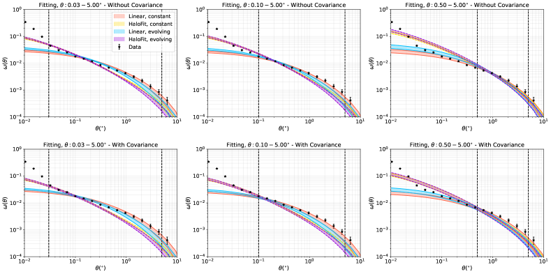
(a) Using method 1 - when each $p(z)$ sample is equally weighted.

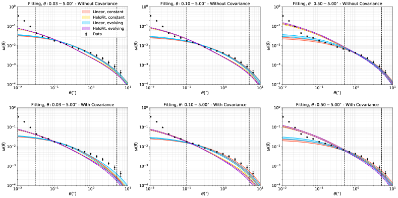
(b) Using method 2 - when each $p(z)$ sample is not equally weighted.

Figure 21: Comparisons of $\omega(\theta)$ for LoTSS-DR2 and their modelled fits (subtracting the integral constraint) assuming errors without accounting for covariance between $\theta$ bins (upper row of each sub figure) and using the full covariance matrix is shown (lower row of each sub figure). These models are shown for the angular fitting ranges $0.03-5\,\deg$ (left), $0.1-5\,\deg$ (centre) and $0.5-5\,\deg$ (right), with the dashed vertical lines indicating the angular scales used for fitting. Black stars correspond to the measurements from LoTSS-DR2, and the shaded regions correspond to (i) the linear constant bias model (red), (ii) the HaloFit constant bias model (yellow), (iii) the linear evolving bias model (blue) and (iv) the HaloFit evolving bias model (purple). The upper panel presents the results when all redshift resamples are weighted equally, whilst the lower panel allows preferential $p(z)$ resamples to be weighted preferentially.

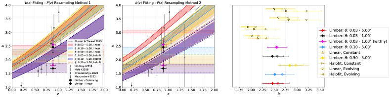
Figure 22: Comparisons of the bias models fit (using the full covariance) for the data for a constant bias model and evolving bias model for the three angular fitting ranges: $0.03-5\,\deg$ (red), $0.1-5\,\deg$ (blue) and $0.5-5\,\deg$ (yellow) for linear (lighter colours) and HaloFit (darker colours) models. The left panel shows the results when each $p(z)$ resamples is weighted as equally probable (method 1, Section 5.2) and the centre panel shows the results when preferential $p(z)$ models are upweighted (method 2, Section 5.2). This is presented alongside previous measurements from Nusser & Tiwari (2015) (grey dashed line), Lindsay et al. (2014a) (grey pentagons), Hale et al. (2018) (grey triangles), Chakraborty et al. (2020) (grey squares) and Mazumder et al. (2022) (grey diamonds). Also shown are the fitting of $b(z)$ from Equation 22 using the angular fitting range 0.03-1^∘ (evaluated at the median redshift of the sample) for the fixed slope ($\gamma$) model (black) and 2 parameter model (magenta) for both the comoving (diamond) and linear (circle) Limber models. The right hand panel shows a comparison of the bias values (evaluated at $z_{med}\approx 0.89$) from CCL (in the 0.5-5^∘ fitting range) using the linear constant (up facing triangle), HaloFit constant (right facing triangle), linear evolving (down facing triangle) and HaloFit evolving (left facing triangle) with and without covariance (indicated by a fainter symbol). The filled markers for the CCL fitting represent those models where the $p(z)$ samples are uniformly weighted and open markers indicate where a preferential $p(z)$ model was preferentially selected. These are presented alongside the Limber comoving linear models across the three angular fitting ranges. Values on the right hand panel are shown with an arbitrary offset on the y-axis to highlight the differences in the values.

$\theta$ Range	Fitting Type	$\textrm{log}_{10}(A)$	$r_{0,c}$ (Mpc)	$b_{c}(z_{m})$	$r_{0,l}$ (Mpc)	$b_{l}(z_{m})$
(∘)
0.03 - 5.00	Without Cov	$-2.50^{+0.01}_{-0.01}$	$11.55^{+0.92}_{-0.77}$	$2.58^{+0.25}_{-0.21}$	$15.41^{+1.99}_{-1.44}$	$1.77^{+0.20}_{-0.14}$
0.10 - 5.00	Without Cov	$-2.47^{+0.01}_{-0.01}$	$12.02^{+0.96}_{-0.81}$	$2.68^{+0.26}_{-0.22}$	$16.04^{+2.06}_{-1.50}$	$1.83^{+0.20}_{-0.15}$
0.50 - 5.00	Without Cov	$-2.38^{+0.02}_{-0.02}$	$13.51^{+1.11}_{-0.96}$	$2.97^{+0.29}_{-0.25}$	$18.03^{+2.33}_{-1.74}$	$2.04^{+0.23}_{-0.17}$
0.03 - 1.00	Without Cov	$-2.50^{+0.01}_{-0.01}$	$11.48^{+0.92}_{-0.77}$	$2.57^{+0.25}_{-0.21}$	$15.32^{+1.97}_{-1.43}$	$1.76^{+0.20}_{-0.14}$
0.03 - 5.00	With Cov	$-2.54^{+0.01}_{-0.01}$	$10.96^{+0.88}_{-0.75}$	$2.46^{+0.24}_{-0.21}$	$14.63^{+1.88}_{-1.38}$	$1.69^{+0.19}_{-0.14}$
0.10 - 5.00	With Cov	$-2.52^{+0.02}_{-0.02}$	$11.22^{+0.91}_{-0.78}$	$2.51^{+0.24}_{-0.21}$	$14.97^{+1.93}_{-1.43}$	$1.72^{+0.19}_{-0.14}$
0.50 - 5.00	With Cov	$-2.42^{+0.03}_{-0.03}$	$12.83^{+1.13}_{-1.01}$	$2.84^{+0.29}_{-0.25}$	$17.14^{+2.26}_{-1.76}$	$1.95^{+0.22}_{-0.18}$
0.03 - 1.00	With Cov	$-2.54^{+0.01}_{-0.01}$	$10.96^{+0.88}_{-0.75}$	$2.46^{+0.24}_{-0.21}$	$14.62^{+1.88}_{-1.38}$	$1.69^{+0.19}_{-0.14}$

Table 3: Results from fitting $\omega(\theta)$ for models across a range of angular fitting ranges. Presented is the fitting range, Fitting type, amplitude of power law ($A$) as in Equation 12, clustering length, $r_{0}$, and bias, $b_{L}$, from Limber inversion using both a comoving (c) and linear (l) assumption. Bias values are evaluated at the median value of the median redshifts ($z_{m}$) from the $p(z)$ resamples, as in Figure 20, $z_{m}\approx 0.89$. This is for both the case where the full covariance matrix is (With Cov) and is not (Without Cov) used.

$\theta$ Range	Fit	$b_{0,L}$	$b_{L}(z_{m})$	$\chi_{L}^{2}$/	$b_{0,H}$	$b_{H}(z_{m})$	$\chi_{H}^{2}$/	$b_{0,L}$	$b_{L}(z_{m})$	$\chi_{L}^{2}$/	$b_{0,H}$	$b_{H}(z_{m})$	$\chi_{H}^{2}$/
(∘)	Type			DOF			DOF	Cov	Cov	DOF	Cov	Cov	DOF
										Cov			Cov
0.03 - 5.00	E/U	$1.90^{+0.10}_{-0.09}$	$2.97^{+0.15}_{-0.15}$	9.34	$1.51^{+0.12}_{-0.10}$	$2.37^{+0.19}_{-0.16}$	13.69	$1.83^{+0.08}_{-0.08}$	$2.87^{+0.13}_{-0.13}$	10.50	$1.41^{+0.11}_{-0.10}$	$2.21^{+0.18}_{-0.15}$	4.43
0.10 - 5.00	E/U	$1.83^{+0.10}_{-0.10}$	$2.87^{+0.16}_{-0.15}$	4.12	$1.57^{+0.13}_{-0.11}$	$2.46^{+0.21}_{-0.17}$	14.58	$1.73^{+0.08}_{-0.08}$	$2.71^{+0.13}_{-0.13}$	2.73	$1.41^{+0.12}_{-0.10}$	$2.21^{+0.18}_{-0.16}$	5.52
0.50 - 5.00	E/U	$2.04^{+0.20}_{-0.17}$	$3.20^{+0.32}_{-0.27}$	3.53	$2.04^{+0.21}_{-0.17}$	$3.20^{+0.33}_{-0.27}$	4.49	$1.79^{+0.15}_{-0.14}$	$2.81^{+0.24}_{-0.22}$	3.18	$1.75^{+0.16}_{-0.15}$	$2.74^{+0.25}_{-0.23}$	4.05
0.03 - 5.00	C/U	$2.37^{+0.19}_{-0.17}$	-	12.74	$1.79^{+0.20}_{-0.15}$	-	11.40	$2.36^{+0.17}_{-0.15}$	-	14.01	$1.68^{+0.19}_{-0.14}$	-	3.95
0.10 - 5.00	C/U	$2.27^{+0.19}_{-0.16}$	-	2.24	$1.87^{+0.22}_{-0.16}$	-	11.62	$2.21^{+0.16}_{-0.15}$	-	3.05	$1.69^{+0.20}_{-0.15}$	-	4.81
0.50 - 5.00	C/U	$2.33^{+0.28}_{-0.22}$	-	1.76	$2.32^{+0.30}_{-0.23}$	-	2.63	$2.14^{+0.22}_{-0.20}$	-	1.81	$2.07^{+0.24}_{-0.20}$	-	2.79
0.03 - 5.00	E/W	$1.98^{+0.05}_{-0.06}$	$3.11^{+0.07}_{-0.10}$	7.81	$1.18^{+0.01}_{-0.01}$	$1.84^{+0.02}_{-0.02}$	10.27	$1.97^{+0.09}_{-0.05}$	$3.09^{+0.14}_{-0.08}$	9.07	$1.35^{+0.08}_{-0.08}$	$2.11^{+0.13}_{-0.13}$	4.19
0.10 - 5.00	E/W	$1.69^{+0.04}_{-0.07}$	$2.66^{+0.06}_{-0.11}$	1.46	$1.21^{+0.06}_{-0.02}$	$1.90^{+0.09}_{-0.03}$	11.49	$1.71^{+0.07}_{-0.06}$	$2.68^{+0.11}_{-0.10}$	2.15	$1.33^{+0.08}_{-0.09}$	$2.09^{+0.13}_{-0.13}$	5.18
0.50 - 5.00	E/W	$1.81^{+0.15}_{-0.12}$	$2.84^{+0.24}_{-0.19}$	1.46	$1.78^{+0.14}_{-0.13}$	$2.79^{+0.22}_{-0.21}$	2.59	$1.67^{+0.12}_{-0.12}$	$2.62^{+0.19}_{-0.18}$	1.86	$1.62^{+0.12}_{-0.11}$	$2.54^{+0.19}_{-0.18}$	3.11
0.03 - 5.00	C/W	$2.77^{+0.17}_{-0.15}$	-	9.54	$1.49^{+0.22}_{-0.18}$	-	9.20	$3.04^{+0.05}_{-0.06}$	-	10.63	$1.67^{+0.17}_{-0.13}$		3.83
0.10 - 5.00	C/W	$2.28^{+0.13}_{-0.11}$		1.68	$1.57^{+0.15}_{-0.20}$	-	10.56	$2.33^{+0.13}_{-0.13}$	-	2.59	$1.65^{+0.18}_{-0.13}$	-	4.65
0.50 - 5.00	C/W	$2.15^{+0.17}_{-0.18}$	-	0.74	$2.10^{+0.18}_{-0.18}$	-	1.67	$2.02^{+0.17}_{-0.16}$	-	1.03	$1.94^{+0.17}_{-0.16}$	-	2.24

Table 4: Results from fitting bias with CCL across a range of angular fitting scales, with both the linear ($b_{L}$) and HaloFit ($b_{H}$) models of CCL. These are both given by their value at $z=0$ and, for the evolving bias model, are evaluated at the median value of the median redshifts ($z_{m}$) from the $p(z)$ resamples, as in Figure 20, $z_{m}\approx 0.89$. These are given for both the case where the full covariance matrix is not used and where it is included (denoted by Cov). For each model the median reduced 2$\chi^{2}$ ($\chi^{2}$/DOF) from the resampled bias values is also given. This will be larger than the best fit model found across the samples, but is provided to show representative values for the fit. A fit type is given by the combination of the bias evolution type (E=evolving, C=constant) and redshift resampling method (U = unweighted i.e. all $p(z)$ samples weighted equally and W = weighted i.e. preferential $p(z)$ resamples are selected).

6 Discussion

In this section we shall discuss our results in context of the different models used to fit the data as well as comparing to previous studies of the angular clustering of radio sources.

6.1 Comparing CCL derived models for $\omega(\theta)$ and $b(z)$

First we compare the fitting of $\omega(\theta)$ using the linear and HaloFit models of CCL. As can be seen in Figure 21, the fit of $\omega(\theta)$ using the linear model appears to have relatively good agreement with the data across the angular range 0.06-1^∘ using all three angular fitting ranges considered in this work when using the more simplistic $\chi^{2}$ for both the evolving and constant bias models. Above 1^∘, the evolving bias model appears to underestimate slightly $\omega(\theta)$, compared to the constant bias model, especially when using fitting ranges that cover the largest angular range and the full covariance is considered. As the full covariance accounts for correlations between different angular bins, this allows the model to under-predict $\omega(\theta)$ on these scales relative to what might be expected by simply looking at minimizing $\chi^{2}$ using the diagonal errors on $\omega(\theta)$ only. However, such an effect is less notable in Figure 21(b) where we allow the $p(z)$ resamples to be preferentially selected to best fit the model. Below 0.06^∘, the measured value for $\omega(\theta)$ appears to be larger than expected from the linear model for both the evolving and constant bias models, with an even larger discrepancy for $\theta<0.03$^∘, where we believe the effect of multi-component sources within the LoTSS-DR2 survey is important. On the contrary, the HaloFit model, shows greater agreement with $\omega(\theta)$ for $\theta\leq 0.06$^∘ when fitting with minimum angular scales $\theta\leq 0.1^{\circ}$. However, in doing so these models greatly underestimate $\omega(\theta)$ on the majority of larger angular scales ($\theta\geq 0.1$^∘), which is where linear bias is dominating. This results in significantly larger reduced $\chi^{2}$ values compared to the linear models. For the narrowest angular fitting range (fitting between 0.5-5^∘), instead, there is much better agreement with the measured $\omega(\theta)$ on the largest angular scales (comparable to that when using a linear model), but the model significantly over predicts the clustering at angles $\lesssim 0.5^{\circ}$.

This comparison suggests that neither the linear or HaloFit models can completely reproduce the measured $\omega(\theta)$ across the full range of angular scales presented in Figure 21, though above the angular scale where we believe the effects of multi-component sources is negligible ($\theta\geq 0.03$^∘), the linear models are able to much more accurately fit the data across a wider range of angular scales using both $p(z)$ resampling methods. The linear and HaloFit models should agree on the largest angular scales and only deviate at small angular scales due to the ‘1-halo’ clustering from sources within the same dark matter halo. When measuring the linear bias, where we measure the ‘2-halo’ clustering relating to galaxies in different dark matter haloes, it is important that the model $\omega(\theta)$ from the fitting be an accurate representation on the largest angular scales. Therefore, the bias measured by the HaloFit models using the angular ranges 0.03-5^∘  and 0.1-5^∘ appears to underestimate $\omega(\theta)$ on the largest angular scales compared to the linear models and so will underestimate the linear bias. These should therefore not be used to draw conclusions of $b_{0}$. When fitting for angular scales of $\theta\geq 0.5$^∘ there is better agreement between the linear and HaloFit models and so measurements of bias from such models are more likely to represent the true bias.

Given that cross-matched data for the LoTSS-DR2 is not currently available for the full LoTSS-DR2 sample, and instead cross-matching is only complete above 8 mJy (Hardcastle et al., 2023), it is not possible to conclusively determine whether we do have a significant contribution of 1-halo clustering to $\omega(\theta)$ in this work. However, from the LoTSS-DR1 clustering measurements shown in Figure 16, the correction for multi-component sources is relatively small and would be insufficient to explain the excess clustering seen here at small angular scales ($\theta\lesssim$0.03^∘). This therefore suggests that we are indeed observing some 1-halo clustering within LoTSS-DR2. Given the uncertainty in the effect of multi-component sources, however, we are also unable to do a full halo occupation distribution modelling (HOD; see e.g. Berlind & Weinberg, 2002; Zheng et al., 2005) in order to determine properties of the haloes which allow them to host multiple radio sources of the type observed in this data.

At the largest angular scales, we note that the linear and HaloFit models are slightly lower than the measured $\omega(\theta)$ from the data when the full covariance is used (especially when uniform weighting is used for each $p(z)$ resample). This may suggest that residual systematics remain within the data which are not fully captured by the randoms but are accounted for by the covariance. Alternatively, it could also represent a contribution of the radio dipole to the observed TPCF, which can cause an excess clustering at larger angular scales (see Chen & Schwarz, 2016), but is not included in our models. More likely, these differences could suggest the assumed bias models used in this analysis may be too simplistic for the sources observed in this work. Our sample is a combination of different sources types and luminosities which dominate at different redshift ranges and so contribute differently across the redshift distribution. Such sub-populations have different bias evolution models (see e.g. Magliocchetti et al., 2017; Hale et al., 2018; Chakraborty et al., 2020; Mazumder et al., 2022), which are complex to combine when considering only a single population. As we are unable to separate the LoTSS-DR2 sources into different source classes we rely on more simplistic models to probe the population as an average population, until the time where such sources can be studied in greater detail, split by source type. Such studies which account for differences in bias models are more beneficial for those data where sources have been associated with a galaxy host, assigned a redshift and source classification has been undertaken to identify the source type. This will be aided in future over such large sky areas with WEAVE-LOFAR (Smith et al., 2016), where spectra can be used to attribute redshifts to sources and to classify the source type. At present, though, such studies should focus on deep, multi-wavelength fields, as in the recent works of Hale et al. (2018); Chakraborty et al. (2020); Mazumder et al. (2022).

Alternatively, if the systematics within the data have been fully accounted for it could imply that the true $p(z)$ is different from that currently estimated from the LoTSS Deep Fields. Figure 23 shows the preferred $p(z)$ models (using a linear model, fit over the angular range 0.5-5^∘), which favour a model with a greater fraction of sources at these low redshifts. As discussed, this provides a much better fit to the data at the largest angular scales than using a uniform weighting of our resampled $p(z)$ models, reflected in the smaller average $\chi^{2}/DOF$ values for our samples. For other angular fitting ranges which may give poorer fits to the data, the preferred $p(z)$ may shift to higher or lower redshifts, however we present the 0.5-5^∘ range which we believe is the most trustworthy to measure linear bias. We note that over the 0.5-5^∘ fitting range, the measured bias values presented in Table 4 are lower using the weighted $p(z)$ resampling, but are consistent with one another within $\sim$ 1$\sigma$. Discerning between whether we expect a $p(z)$ with a stronger preference to low redshift sources or that there are residual systematics in our data is challenging, but will be aided with future spectroscopic surveys such as WEAVE-LOFAR (Smith et al., 2016).

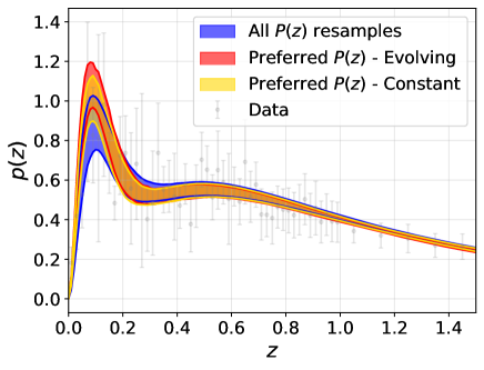
Figure 23: $p(z)$ for the data (grey) compared to the range of $p(z)$ models when uniformly sampling the data (blue) compared to allowing the $p(z)$ resamples to preferentially selected in the fitting process (see Section 5.2) for a linear model across the angular range 0.5-5^∘ using the full covariance array with an evolving (red) and constant (yellow) bias model. All models are shown in the range given by the 16th and 84th percentiles.

Next, we consider the comparison between the evolving, $b(z)=b_{0}/D(z)$, and constant, $b(z)=b_{0}$, bias models for our data, as presented in Figure 22. The model used in analysis of NVSS in Nusser & Tiwari (2015) was an evolving bias model and we also note that for previous measurements using Limber inversion, the choice of comoving clustering assumes a non-evolving $r_{0}$ and so an evolving bias model inversely proportional to the growth factor, as can be seen in Equation 22. As can be seen in Figure 21, both the evolving and constant bias model appear to accurately recreate the observed angular TPCF across a diverse range of angular scales ($\sim 0.07-1^{\circ}$). However, whilst at $\theta\sim 1-5^{\circ}$ the model for $\omega(\theta)$ using the constant bias model (and assuming equal weighting for our $p(z)$ resamples, see Figure 21(a)) can be seen to better model $\omega(\theta)$ at the largest angular scales, the evolving bias model under predicts the observed angular-two-point correlation function. This would therefore imply that a constant bias model appears to more accurately represent the measurements made in this work. However, in the literature, bias models which evolve and increase with redshift have typically been assumed due to expectations that at higher redshifts a halo of the same mass represents a more extreme fluctuation from the average, and so is more biased. In SKADS (Wilman et al., 2008), the authors used an assumption of a constant mass haloes for each different source population, these result in an evolving bias model for such an assumption. These models have been used in numerous cosmology forecasts (Raccanelli et al., 2012; Ferramacho et al., 2014; Square Kilometre Array Cosmology Science Working Group et al., 2020). The model used in the analysis presented in this work, however, includes a more simplistic evolving bias model, inversely proportional to the growth factor, and more complicated evolutionary models taking into account the contributions of different source populations are likely more appropriate. If the $p(z)$ resamples are allowed to be preferentially chosen to best fit the data (see Figure 21(b)), the constant and evolving bias models both appear to become more similar compared to the measurements of $\omega(\theta)$.

Finally, comparisons can be made for the results when using the full covariance matrix, compared to errors based on the diagonals of the covariance matrix. Work such as Lindsay et al. (2014a) and Hale et al. (2018) have followed methods where only the uncertainties on a $\theta$ bin and not the full covariance matrix was assumed, which could affect the measurements of bias. As can be seen in Figures 21-22 and in Tables 3-4, there do exist differences in the measured bias and $\omega(\theta)$ models depending on whether or not the full covariance matrix is provided. These often find a lower bias value when the full covariance matrix is used, although the values are typically consistent within 1-2$\sigma$. Differences between the results with and without the full covariance imply a correlation between angular scales which needs to be accounted for in the fitting of $\omega(\theta)$. We therefore use the models in which the full covariance is incorporated for drawing conclusions. We also note that when weighting all $p(z)$ resamples equally (and modelling these as in Equation 15), the results when using the covariance matrix from TreeCorr (with $N_{\textrm{Jack}}=100$) were consistent within $\sim 1\sigma$ and using a $\delta z=0.1$ binning for the $p(z)$ from the LoTSS Deep fields also resulted in $b_{0}$ values consistent within $\sim 1-1.5\sigma$ to those presented in this work.

6.2 Comparison of $b(z)$ to other surveys

We next present comparisons to the results made from previous measurements with similar large area surveys. As this work follows from the previous work of LoTSS-DR1 presented in Siewert et al. (2020), we first make comparisons to the results found in that work. In Siewert et al. (2020), redshifts were not available for the full population of LoTSS-DR1 sources and no redshift data for LOFAR sources in the Deep Fields were available at that time. Therefore for bias measurements this relied on those sources which had cross-matched hosts (from Williams et al., 2019) and redshifts (from Duncan et al., 2019). This meant that approximately 50% of sources had redshifts available, but that measurements of bias in redshift bins were skewed to those sources. Therefore it is challenging to make direct comparisons to that work. However, it is possible to make comparisons to the fitting parameters for $\omega(\theta)$ provided in Siewert et al. (2020).

In Figure 24 we present comparisons of the best fit models to Siewert et al. (2020) as well as a number of other previous works from Lindsay et al. (2014a); Hale et al. (2019); Bonato et al. (2021) and Mazumder et al. (2022). For these works we include an indication of the equivalent flux limit used, scaled to 144 MHz. For those with fainter populations we note that differences in the populations being observed, which will be increasingly dominated by SFGs below $1\,\mathrm{mJy}$, will affect the comparison of such measurements. As can be seen from Figure 24, our work finds a smaller clustering amplitude to that found in Mask 1 used in Siewert et al. (2020) at $2\,\mathrm{mJy}$ (their best model from their paper). We do note that our result is in excellent agreement to that of Siewert et al. (2020) using their $2\,\mathrm{mJy}$ cut in Mask d (not shown in Figure 24), which used a less conservative masking of regions they considered to have ‘good’ sensitivity. As discussed though in Section 3.3.4, there are differences introduced in this work for the method of generating random sources compared to that in Siewert et al. (2020), which may also affect comparisons of the measurements, as systematics in the data were accounted for using some different methods.

At both similar flux densities and a similar frequency to this work is the clustering presented in Hale et al. (2019). In their work, the clustering of sources within the XMM-LSS field as observed with LOFAR was presented, and Hale et al. (2019) found a clustering amplitude approximately three times larger to the work presented here. These difference could arise from cosmic variance as the XMM-LSS field covers a much smaller area ($\sim$25 sq. deg) compared to the $\sim$5000 sq. deg used in this work. However, we also note that Hale et al. (2019) discuss the fact that the corrected source counts appear to suggest that the completeness corrections applied are an underestimation. This could affect the measurement of $\omega(\theta)$ in their work. Our work is consistent with that of Lindsay et al. (2014a) who study the clustering of sources in FIRST (Becker et al., 1995; Helfand et al., 2015) with an equivalent limit at 144 MHz of $\sim 5\,\mathrm{mJy}$, yet there are large uncertainties in their work. We derive a larger amplitude than that of Mazumder et al. (2022), who use 325 MHz observations of the Lockman Hole field which are the equivalent of $\sim$3$\times$ more sensitive than for LoTSS-DR2, but restricted over smaller areas. Whilst previous work has investigated how the amplitude of clustering changes with flux density (see e.g. Wilman et al., 2003; Overzier et al., 2003), who find a typical declining amplitude at smaller flux densities, the complication between the different populations introduced and changes in redshift distribution as flux limits decrease means that discussion of the power law amplitude is complicated to make direct comparisons. We provide the inset in Figure 24 to show the flux density dependence in context with the other work presented.

Next, comparing the bias evolution models implied from this work to those from other works, we note that again there exists challenges when making comparisons due to the variety of radio populations, and their variation with flux density. Radio surveys are dominated by AGN at the brightest flux densities, with SFG dominating at fainter flux densities (see e.g. Smolčić et al., 2017b; Algera et al., 2020; Hale et al., 2023) and Best et al. (2023). For example, Nusser & Tiwari (2015) used a quadratic polynomial model to investigate an evolving bias model for NVSS sources with $S_{1.4\textrm{GHz}}\geq 2.5\,\mathrm{mJy}$. This is an equivalent flux density limit of $\sim 12.5\,\mathrm{mJy}$ at $144\,\mathrm{MHz}$, approximately 8$\times$ the flux density limit used in this work. These sources will be dominated by AGN and have very little contribution of SFG, whereas we expect a much larger contribution of SFGs within this work. As shown in radio clustering studies such as Magliocchetti et al. (2017); Hale et al. (2018) and Mazumder et al. (2022), these two populations are believed to have different biases and so by investigating the bias for a source population as a whole, the bias measured will be an average between the bias of the two populations. Moreover, if such previous studies use comoving clustering, these should be compared to the evolving bias models instead of a constant bias model. Therefore the results shown for the Limber derived bias values for comoving clustering in this work are only comparable for the evolving bias model and not the constant model. Our measurements of bias with Limber’s equation (when assuming a power law spatial clustering model) can underestimate the bias model (if comparing to those from CCL), though these are typically consistent within 1-2$\sigma$. The remaining differences highlight the challenges when making comparisons of bias evolution models using these different approaches. .

Evolving bias models (with the covariance) are consistent with some of the measured values from Chakraborty et al. (2020) and Hale et al. (2018) as well as the evolving bias model from NVSS (Nusser & Tiwari, 2015), especially when the linear model is assumed. We note that whilst for Hale et al. (2018) we present results for the full population in Figure 22, the results for Chakraborty et al. (2020); Mazumder et al. (2022) are separated by source type, with those for SFGs found to have lower bias values. Therefore our agreement with Chakraborty et al. (2020) is to their AGN population measurements and similarly, as discussed, NVSS will also be dominated by AGN at the flux densities applied. Recent work from Best et al. (2023) for the LoTSS Deep Fields, suggests $\sim$20% of SFGs and $\sim$6% of radio quiet quasars (RQQs, which become more important at faint flux densities, see e.g. Jarvis & Rawlings, 2004) at the limiting flux density used in this work.

It is also important to compare to the results of Alonso et al. (2021) who used a combination of LoTSS-DR1 and CMB measurements to jointly constrain both $p(z)$ and $b(z)$ (for sources $\geq$2 mJy). Their results suggested that for an evolving bias model the value of $b_{0}$ is expected to be $\sim$1.2-1.7, assuming a redshift distribution similar to that of Smolčić et al. (2017b) using an appropriate flux density cut. Our measurements over the 0.5-5^∘ angular fitting range using the full covariance matrix to determine $b_{0}$ are slightly larger than the results of Alonso et al. (2021) (when the $p(z)$ samples are equally weighted), though our results are consistent with their upper limits within our 1$\sigma$ uncertainties. However, when we allow more preferential $p(z)$ models to be weighted, we find $b_{0}\sim 1.6-1.7$, consistent with the work of Alonso et al. (2021). In their work, Alonso et al. (2021) fit for both the $p(z)$ and $b(z)$ model, and so are more comparable to when we allow preferential selection of the $p(z)$ samples. For the constant bias models, on the other hand, our $b_{0}$ values are typically lower than those found in (Alonso et al., 2021, who find $b_{0}\sim 2.3-4$). However, their redshift distribution which they find for such a constant bias model is skewed to a much higher redshift than shown in Figure 20. Our redshift distribution peaks significantly below $z\sim 1$, similar to the evolving bias model of Alonso et al. (2021), whereas their constant bias model predicts a redshift distribution peaking at $z\sim 1-2$. From Figure 23, we see that the LoTSS Deep Fields data do not indicate such a peak at higher redshifts. Therefore, to have agreement between this work and that of Alonso et al. (2021) this suggests a preference towards an evolving bias model for LoTSS sources assuming a redshift distribution similar to that of the LoTSS Deep Fields.

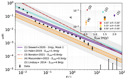
Figure 24: Comparison of the $\omega(\theta)$ from this work (black stars) compared to previous power law fitting from the studies of Siewert et al. (2020) using a $2\,\mathrm{mJy}$ (solid purple) cut as well as the works of Hale et al. (2019) (turquoise dotted), Bonato et al. (2021) (dark red dot-dashed), Mazumder et al. (2022) (orange dashed) and Lindsay et al. (2014a) (light grey dotted). Inset: Amplitude variation as a function of flux density compared to the fitting here using the simple $\chi^{2}$ method across the three fitting ranges: 0.03-5.00^∘ (red), 0.10-5.00^∘ (yellow) and 0.50-5.00^∘ (black). The quoted flux limits are scaled to 144 MHz to allow more equivalent comparisons.

7 Conclusions

The LOFAR Two-metre Sky Survey Data Release 2 (LoTSS-DR2; Shimwell et al., 2022) provides a catalogue of $\sim$4.4 million low frequency radio sources over $\sim 5600\,\deg^{2}$, making it an ideal data set for radio cosmology studies of the large-scale structure of the Universe. In this work we provided analysis of the angular clustering of sources in the LoTSS-DR2 survey and comparison of the bias models implied for such sources. We provide a comprehensive description of the methods used to improve upon the accuracy of the random catalogues generated in this work compared to those used in the LoTSS-DR1 clustering analysis of Siewert et al. (2020). Our random catalogues account for a variety of observational biases within the data including: rms sensitivity variations across the field of view; resolution bias; smearing variations across the observations; detection completeness of PyBDSF; and the effect of Eddington and measurement biases on the measured flux density properties of sources.

Using the random catalogues generated we measure the angular two-point correlation function, $\omega(\theta)$, for sources with SNR$\geq$7.5 and integrated flux density $\geq$$1.5\,\mathrm{mJy}$, which shows an approximate power law behaviour ($\omega(\theta)\propto\theta^{1-\gamma}$) over the angular scales between 0.03 and 2^∘. We model $\omega(\theta)$ using a variety of models which account for both an evolving and constant bias model as well as using matter power spectrum models which account for linear effects only (‘linear’) or with non-linear effects also included (‘HaloFit’). Our results show that in order to best model the $\omega(\theta)$ measured from LoTSS-DR2 across a range of angular scales ($\sim 0.1-1^{\circ}$), the linear model is preferred, which suggests that at the sensitivities probed by this work, we are typically only observing a single radio source per dark matter halo, and do not have a strong contribution from ‘1-halo’ clustering. However, we note that the linear model underestimates the clustering at smaller angular scales, where a combination of 1-halo clustering and multi-component source clustering may play a role.

Comparing bias evolutionary models with the linear halo model, assuming the models based on the redshift distributions from the LoTSS Deep Fields accurately represent that of our data, our work suggests that for an evolving bias model of the form $b(z)=b_{0}/D(z)$, the best fit value of $b_{0}\sim 1.7-1.8$ over the angular scales which we believe are most accurate for measuring bias (0.5-5^∘). Instead for a constant bias model, of the form $b(z)=b_{0}$, we find $b_{0}\sim 2.1$. At the largest angles ($\geq 1^{\circ}$), we see that the constant bias model provides a slightly better fit to the observed data when we use equally weighted $p(z)$ models from the LoTSS Deep fields to measure bias. Such differences are reduced if we allow our models to have preferential $p(z)$ models, based on the fit to the data. Where we allow our $p(z)$ model to be preferentially selected, the bias values in both the constant and evolving bias models also reduced slightly, to $b_{0}\sim 1.6-1.7$ in an evolving model, and $b_{0}\sim 2.0$ for a constant model. Assuming an evolving bias model and taking into account the full covariance matrix, we find good agreement with the results from NVSS of Nusser & Tiwari (2015) up to $z\sim 1$ and previous results from Hale et al. (2018); Chakraborty et al. (2020), though we note that these probe different populations at both different frequencies and different equivalent sensitivities to that used in this work.

Moreover, in comparison with work from LoTSS-DR1 of Alonso et al. (2021) who used both CMB and LOFAR measurements to jointly constrain the redshift distribution and bias evolution model of LoTSS-DR1 sources ($\geq$2 mJy), we find that given the greater knowledge of the redshift distributions contributed by the LoTSS Deep Fields (see Sabater et al., 2021; Tasse et al., 2021; Duncan et al., 2021), an evolving model from Alonso et al. (2021) is necessary to reflect the redshift distribution found in their work. We find that the bias values presented from Alonso et al. (2021) for their evolving model is similar to that of the evolving bias models presented in this work, especially when we allow $p(z)$ models to be preferentially determined during the fitting process. Using a linear model for the matter power spectrum to fit across the largest angular scales (0.5-5^∘) and equally weighting $p(z)$ models from the LoTSS Deep Fields, we find, for an evolving bias model, a value of $b_{0}=1.79^{+0.15}_{-0.14}$ which is equivalent to $b_{E}=2.81^{+0.24}_{-0.22}$ at the median redshift of our sample, $z_{\mathrm{m}}\approx 0.9$ when we do not show a preference to the $p(z)$ models, reducing to $b_{0,E}=1.67^{+0.12}_{-0.12}$ which is equivalent to $b_{E}=2.62^{+0.19}_{-0.18}$ and $b_{0,C}=2.02^{+0.17}_{-0.16}$ when we allow our measurements to suggest preferential $p(z)$ models, which are found to peak more strongly at lower redshifts.

Observations from future spectroscopic surveys such as WEAVE-LOFAR (Smith et al., 2016) will allow us to more accurately determine the redshift distribution of LOFAR sources at low redshifts and allow more understanding of the $p(z)$ models we expect for the sources observed in this work. This will allow us to disentangle whether small systematics remain within our data or we have a population of radio sources which are more highly skewed to low redshifts (e.g. from SFGs). As the low redshift $p(z)$ appears important for this work in modelling $\omega(\theta)$ at the larger angular scales, such accurate redshifts at $z<1$ are important for constraining the results of future studies. This work has highlighted how a number of observational systematics can be corrected for future deep radio cosmology studies, whilst also demonstrating that the understanding of systematics in wide field mosaiced images is complex, and needs deep understanding for use in cosmological studies.

Data Availability

LoTSS-DR2 catalogue data is available to the community; for more details on the data used in this work please see Shimwell et al. (2022). LoTSS Deep Fields data is also available publicly, with further information available in Sabater et al. (2021); Tasse et al. (2021); Kondapally et al. (2021); Duncan et al. (2021). Further information can also be found at https://lofar-surveys.org/index.html. Other data presented in this article can be made available upon reasonable request to the author.

References

- Aird & Coil (2021) Aird J., Coil A. L., 2021, MNRAS, 502, 5962
- Alegre et al. (2022) Alegre L., et al., 2022, MNRAS, 516, 4716
- Algera et al. (2020) Algera H. S. B., et al., 2020, ApJ, 903, 139
- Allison et al. (2015) Allison R., et al., 2015, MNRAS, 451, 849
- Alonso et al. (2021) Alonso D., Bellini E., Hale C., Jarvis M. J., Schwarz D. J., 2021, MNRAS, 502, 876
- Astropy Collaboration et al. (2013) Astropy Collaboration et al., 2013, A&A, 558, A33
- Astropy Collaboration et al. (2018) Astropy Collaboration et al., 2018, AJ, 156, 123
- Banfield et al. (2015) Banfield J. K., et al., 2015, MNRAS, 453, 2326
- Barkus et al. (2022) Barkus B., et al., 2022, MNRAS, 509, 1
- Barrow et al. (1984) Barrow J. D., Bhavsar S. P., Sonoda D. H., 1984, MNRAS, 210, 19
- Becker et al. (1995) Becker R. H., White R. L., Helfand D. J., 1995, ApJ, 450, 559
- Berlind & Weinberg (2002) Berlind A. A., Weinberg D. H., 2002, ApJ, 575, 587
- Best et al. (2023) Best P. N., et al., 2023, MNRAS, 523, 1729
- Blake & Wall (2002) Blake C., Wall J., 2002, MNRAS, 337, 993
- Bonaldi et al. (2016) Bonaldi A., Harrison I., Camera S., Brown M. L., 2016, MNRAS, 463, 3686
- Bonaldi et al. (2019) Bonaldi A., Bonato M., Galluzzi V., Harrison I., Massardi M., Kay S., De Zotti G., Brown M. L., 2019, MNRAS, 482, 2
- Bonaldi et al. (2023) Bonaldi A., Hartley P., Ronconi T., De Zotti G., Bonato M., 2023, MNRAS, 524, 993
- Bonato et al. (2021) Bonato M., Prandoni I., De Zotti G., Brienza M., Morganti R., Vaccari M., 2021, MNRAS, 500, 22
- Bridle & Schwab (1999) Bridle A. H., Schwab F. R., 1999, in Taylor G. B., Carilli C. L., Perley R. A., eds, Astronomical Society of the Pacific Conference Series Vol. 180, Synthesis Imaging in Radio Astronomy II. p. 371
- Brodwin et al. (2008) Brodwin M., et al., 2008, ApJ, 687, L65
- Callingham et al. (2017) Callingham J. R., et al., 2017, ApJ, 836, 174
- Ceverino & Klypin (2009) Ceverino D., Klypin A., 2009, ApJ, 695, 292
- Chakraborty et al. (2020) Chakraborty A., Dutta P., Datta A., Roy N., 2020, MNRAS, 494, 3392
- Chambers et al. (2016) Chambers K. C., et al., 2016, arXiv e-prints, p. arXiv:1612.05560
- Chen & Schwarz (2016) Chen S., Schwarz D. J., 2016, A&A, 591, A135
- Chisari et al. (2019) Chisari N. E., et al., 2019, ApJS, 242, 2
- Cochrane et al. (2017) Cochrane R. K., Best P. N., Sobral D., Smail I., Wake D. A., Stott J. P., Geach J. E., 2017, MNRAS, 469, 2913
- Colless et al. (2001) Colless M., et al., 2001, MNRAS, 328, 1039
- Cress et al. (1996) Cress C. M., Helfand D. J., Becker R. H., Gregg M. D., White R. L., 1996, ApJ, 473, 7
- Desjacques et al. (2018) Desjacques V., Jeong D., Schmidt F., 2018, Phys. Rep., 733, 1
- Doroshkevich et al. (2004) Doroshkevich A., Tucker D. L., Allam S., Way M. J., 2004, A&A, 418, 7
- Duncan et al. (2019) Duncan K. J., et al., 2019, A&A, 622, A3
- Duncan et al. (2021) Duncan K. J., et al., 2021, A&A, 648, A4
- Eddington (1913) Eddington A. S., 1913, MNRAS, 73, 359
- Fabian (2012) Fabian A. C., 2012, ARA&A, 50, 455
- Ferramacho et al. (2014) Ferramacho L. D., Santos M. G., Jarvis M. J., Camera S., 2014, MNRAS, 442, 2511
- Foreman-Mackey (2016) Foreman-Mackey D., 2016, The Journal of Open Source Software, 1, 24
- Foreman-Mackey et al. (2013) Foreman-Mackey D., Hogg D. W., Lang D., Goodman J., 2013, PASP, 125, 306
- Galvin et al. (2020) Galvin T. J., et al., 2020, MNRAS, 497, 2730
- Gehrels (1986) Gehrels N., 1986, ApJ, 303, 336
- Gomes et al. (2020) Gomes Z., Camera S., Jarvis M. J., Hale C., Fonseca J., 2020, MNRAS, 492, 1513
- Górski et al. (2005) Górski K. M., Hivon E., Banday A. J., Wandelt B. D., Hansen F. K., Reinecke M., Bartelmann M., 2005, ApJ, 622, 759
- Hale et al. (2018) Hale C. L., Jarvis M. J., Delvecchio I., Hatfield P. W., Novak M., Smolčić V., Zamorani G., 2018, MNRAS, 474, 4133
- Hale et al. (2019) Hale C. L., et al., 2019, A&A, 622, A4
- Hale et al. (2021) Hale C. L., et al., 2021, Publ. Astron. Soc. Australia, 38, e058
- Hale et al. (2023) Hale C. L., et al., 2023, MNRAS, 520, 2668
- Hamilton (2001) Hamilton A. J. S., 2001, MNRAS, 322, 419
- Hancock et al. (2018) Hancock P. J., Trott C. M., Hurley-Walker N., 2018, Publ. Astron. Soc. Australia, 35, e011
- Hardcastle et al. (2023) Hardcastle M. J., et al., 2023, arXiv e-prints, p. arXiv:2309.00102
- Harris et al. (2020) Harris C. R., et al., 2020, Nature, 585, 357
- Helfand et al. (2015) Helfand D. J., White R. L., Becker R. H., 2015, ApJ, 801, 26
- Hill et al. (2008) Hill G. J., et al., 2008, in Kodama T., Yamada T., Aoki K., eds, Astronomical Society of the Pacific Conference Series Vol. 399, Panoramic Views of Galaxy Formation and Evolution. p. 115 (arXiv:0806.0183), doi:10.48550/arXiv.0806.0183
- Hopkins et al. (2012) Hopkins P. F., Quataert E., Murray N., 2012, MNRAS, 421, 3522
- Hunter (2007) Hunter J. D., 2007, Computing in Science and Engineering, 9, 90
- Jarvis (2015) Jarvis M., 2015, TreeCorr: Two-point correlation functions, Astrophysics Source Code Library, record ascl:1508.007 (ascl:1508.007)
- Jarvis & Rawlings (2004) Jarvis M. J., Rawlings S., 2004, New Astron. Rev., 48, 1173
- Kaiser (1984) Kaiser N., 1984, ApJ, 284, L9
- Kellermann et al. (1969) Kellermann K. I., Pauliny-Toth I. I. K., Williams P. J. S., 1969, ApJ, 157, 1
- Kondapally et al. (2021) Kondapally R., et al., 2021, A&A, 648, A3
- Koutoulidis et al. (2013) Koutoulidis L., Plionis M., Georgantopoulos I., Fanidakis N., 2013, MNRAS, 428, 1382
- Landy & Szalay (1993) Landy S. D., Szalay A. S., 1993, ApJ, 412, 64
- Lesgourgues (2011) Lesgourgues J., 2011, arXiv e-prints, p. arXiv:1104.2932
- Lewis et al. (2000) Lewis A., Challinor A., Lasenby A., 2000, ApJ, 538, 473
- Limber (1953) Limber D. N., 1953, ApJ, 117, 134
- Limber (1954) Limber D. N., 1954, ApJ, 119, 655
- Lindsay et al. (2014a) Lindsay S. N., et al., 2014a, MNRAS, 440, 1527
- Lindsay et al. (2014b) Lindsay S. N., Jarvis M. J., McAlpine K., 2014b, MNRAS, 440, 2322
- Ling et al. (1986) Ling E. N., Frenk C. S., Barrow J. D., 1986, MNRAS, 223, 21
- Magliocchetti et al. (1999) Magliocchetti M., Maddox S. J., Lahav O., Wall J. V., 1999, MNRAS, 306, 943
- Magliocchetti et al. (2004) Magliocchetti M., et al., 2004, MNRAS, 350, 1485
- Magliocchetti et al. (2017) Magliocchetti M., Popesso P., Brusa M., Salvato M., Laigle C., McCracken H. J., Ilbert O., 2017, MNRAS, 464, 3271
- Mandal et al. (2021) Mandal S., et al., 2021, A&A, 648, A5
- Massaro et al. (2014) Massaro F., Giroletti M., D’Abrusco R., Masetti N., Paggi A., Cowperthwaite P. S., Tosti G., Funk S., 2014, ApJS, 213, 3
- Matthews et al. (2021) Matthews A. M., Condon J. J., Cotton W. D., Mauch T., 2021, ApJ, 909, 193
- Mauch et al. (2003) Mauch T., Murphy T., Buttery H. J., Curran J., Hunstead R. W., Piestrzynski B., Robertson J. G., Sadler E. M., 2003, MNRAS, 342, 1117
- Mazumder et al. (2022) Mazumder A., Chakraborty A., Datta A., 2022, MNRAS, 517, 3407
- Mo & White (1996) Mo H. J., White S. D. M., 1996, MNRAS, 282, 347
- Mohan & Rafferty (2015) Mohan N., Rafferty D., 2015, PyBDSF: Python Blob Detection and Source Finder, Astrophysics Source Code Library, record ascl:1502.007 (ascl:1502.007)
- Morabito et al. (2022) Morabito L. K., et al., 2022, A&A, 658, A1
- Morganti (2017) Morganti R., 2017, Frontiers in Astronomy and Space Sciences, 4, 42
- Negrello et al. (2006) Negrello M., Magliocchetti M., De Zotti G., 2006, MNRAS, 368, 935
- Norberg et al. (2009) Norberg P., Baugh C. M., Gaztañaga E., Croton D. J., 2009, MNRAS, 396, 19
- Nusser & Tiwari (2015) Nusser A., Tiwari P., 2015, ApJ, 812, 85
- O’Dea & Saikia (2021) O’Dea C. P., Saikia D. J., 2021, A&ARv, 29, 3
- Overzier et al. (2003) Overzier R. A., Röttgering H. J. A., Rengelink R. B., Wilman R. J., 2003, A&A, 405, 53
- Peebles (1975) Peebles P. J. E., 1975, ApJ, 196, 647
- Peebles (1980) Peebles P. J. E., 1980, The large-scale structure of the universe
- Planck Collaboration et al. (2020) Planck Collaboration et al., 2020, A&A, 641, A6
- Prescott et al. (2018) Prescott M., et al., 2018, MNRAS, 480, 707
- Puccetti et al. (2006) Puccetti S., et al., 2006, A&A, 457, 501
- Raccanelli et al. (2012) Raccanelli A., et al., 2012, MNRAS, 424, 801
- Roche & Eales (1999) Roche N., Eales S. A., 1999, MNRAS, 307, 703
- Sabater et al. (2021) Sabater J., et al., 2021, A&A, 648, A2
- Shimwell et al. (2017) Shimwell T. W., et al., 2017, A&A, 598, A104
- Shimwell et al. (2019) Shimwell T. W., et al., 2019, A&A, 622, A1
- Shimwell et al. (2022) Shimwell T. W., et al., 2022, A&A, 659, A1
- Siewert et al. (2020) Siewert T. M., et al., 2020, A&A, 643, A100
- Smith et al. (2003) Smith R. E., et al., 2003, MNRAS, 341, 1311
- Smith et al. (2016) Smith D. J. B., et al., 2016, in Reylé C., Richard J., Cambrésy L., Deleuil M., Pécontal E., Tresse L., Vauglin I., eds, SF2A-2016: Proceedings of the Annual meeting of the French Society of Astronomy and Astrophysics. pp 271–280 (arXiv:1611.02706), doi:10.48550/arXiv.1611.02706
- Smolčić et al. (2017a) Smolčić V., et al., 2017a, A&A, 602, A1
- Smolčić et al. (2017b) Smolčić V., et al., 2017b, A&A, 602, A2
- Springel et al. (2006) Springel V., Frenk C. S., White S. D. M., 2006, Nature, 440, 1137
- Square Kilometre Array Cosmology Science Working Group et al. (2020) Square Kilometre Array Cosmology Science Working Group et al., 2020, Publ. Astron. Soc. Australia, 37, e007
- Starikova et al. (2012) Starikova S., Berta S., Franceschini A., Marchetti L., Rodighiero G., Vaccari M., Vikhlinin A., 2012, ApJ, 751, 126
- Sweijen et al. (2022) Sweijen F., et al., 2022, Nature Astronomy, 6, 350
- Takahashi et al. (2012) Takahashi R., Sato M., Nishimichi T., Taruya A., Oguri M., 2012, ApJ, 761, 152
- Tasse et al. (2021) Tasse C., et al., 2021, A&A, 648, A1
- Taylor (2005) Taylor M. B., 2005, in Shopbell P., Britton M., Ebert R., eds, Astronomical Society of the Pacific Conference Series Vol. 347, Astronomical Data Analysis Software and Systems XIV. p. 29
- Taylor (2011) Taylor M., 2011, TOPCAT: Tool for OPerations on Catalogues And Tables (ascl:1101.010)
- Tinker et al. (2010) Tinker J. L., Robertson B. E., Kravtsov A. V., Klypin A., Warren M. S., Yepes G., Gottlöber S., 2010, ApJ, 724, 878
- Tiwari et al. (2022) Tiwari P., Zhao R., Zheng J., Zhao G.-B., Bacon D., Schwarz D. J., 2022, Astrophys. J., 928, 38
- Totsuji & Kihara (1969) Totsuji H., Kihara T., 1969, PASJ, 21, 221
- Virtanen et al. (2020) Virtanen P., et al., 2020, Nature Methods, 17, 261
- Wang et al. (2013) Wang Y., Brunner R. J., Dolence J. C., 2013, MNRAS, 432, 1961
- Whiting & Humphreys (2012) Whiting M., Humphreys B., 2012, Publ. Astron. Soc. Australia, 29, 371
- Williams et al. (2016) Williams W. L., et al., 2016, MNRAS, 460, 2385
- Williams et al. (2019) Williams W. L., et al., 2019, A&A, 622, A2
- Wilman et al. (2003) Wilman R. J., Röttgering H. J. A., Overzier R. A., Jarvis M. J., 2003, MNRAS, 339, 695
- Wilman et al. (2008) Wilman R. J., et al., 2008, MNRAS, 388, 1335
- Wilman et al. (2010) Wilman R. J., Jarvis M. J., Mauch T., Rawlings S., Hickey S., 2010, MNRAS, 405, 447
- Wright et al. (2010) Wright E. L., et al., 2010, AJ, 140, 1868
- Zehavi et al. (2004) Zehavi I., et al., 2004, ApJ, 608, 16
- Zehavi et al. (2011) Zehavi I., et al., 2011, ApJ, 736, 59
- Zheng et al. (2005) Zheng Z., et al., 2005, ApJ, 633, 791
- Zonca et al. (2020) Zonca A., Singer L., Lenz D., Reinecke M., Rosset C., Hivon E., Gorski K., 2020, healpy: Python wrapper for HEALPix, Astrophysics Source Code Library, record ascl:2008.022 (ascl:2008.022)
- da Costa-Luis et al. (2021) da Costa-Luis C., et al., 2021, tqdm: A fast, Extensible Progress Bar for Python and CLI, doi:10.5281/zenodo.5109730, https://doi.org/10.5281/zenodo.5109730
- de Gasperin et al. (2018) de Gasperin F., Intema H. T., Frail D. A., 2018, MNRAS, 474, 5008
- de Gasperin et al. (2021) de Gasperin F., et al., 2021, A&A, 648, A104
- van Haarlem et al. (2013) van Haarlem M. P., et al., 2013, A&A, 556, A2
- van Weeren et al. (2016) van Weeren R. J., et al., 2016, ApJS, 223, 2
- van der Vlugt et al. (2021) van der Vlugt D., et al., 2021, ApJ, 907, 5
- van der Walt et al. (2011) van der Walt S., Colbert S. C., Varoquaux G., 2011, Computing in Science and Engineering, 13, 22