Unsupervised Learning of Sea Surface Height Interpolation from Multi-variate Simulated Satellite Observations.

Abstract

Satellite-based remote sensing missions have revolutionized our understanding of the Ocean state and dynamics. Among them, spaceborne altimetry provides valuable measurements of Sea Surface Height (SSH), which is used to estimate surface geostrophic currents. However, due to the sensor technology employed, important gaps occur in SSH observations. Complete SSH maps are produced by the altimetry community using linear Optimal Interpolations (OI) such as the widely-used Data Unification and Altimeter Combination System (DUACS). However, OI is known for producing overly smooth fields and thus misses some mesostructures and eddies. On the other hand, Sea Surface Temperature (SST) products have much higher data coverage and SST is physically linked to geostrophic currents through advection. We design a realistic twin experiment to emulate the satellite observations of SSH and SST to evaluate interpolation methods. We introduce a deep learning network able to use SST information, and a trainable in two settings: one where we have no access to ground truth during training and one where it is accessible. Our investigation involves a comparative analysis of the aforementioned network when trained using either supervised or unsupervised loss functions. We assess the quality of SSH reconstructions and further evaluate the network’s performance in terms of eddy detection and physical properties. We find that it is possible, even in an unsupervised setting to use SST to improve reconstruction performance compared to SST-agnostic interpolations. We compare our reconstructions to DUACS’s and report a decrease of 41% in terms of root mean squared error.

Journal of Advances of Modelling Earth Systems (JAMES)

LIP6, Sorbonne University, 4 place Jussieu, Paris, France LOCEAN, Sorbonne University, 4 place Jussieu, Paris, France ENSIIE, Evry, France, LaMME INRIA Paris, Paris, France

Théo Archambaulttheo.archambault@lip6.fr

This is the preprint of a paper submitted to the Journal of Advances of Modelling Earth Systems (JAMES) in September 2023

We developed a realistic simulation of satellite observations of sea surface height and temperature

We compare deep learning supervised and unsupervised strategies to interpolate the sea surface height, and able to use temperature data

We find temperature, enhances sea surface height reconstruction, as well as the estimation of the surface currents and mesoscale eddies.

Plain Language Summary

The surface of the ocean is observed through various sensors embedded in satellites. Specifically, the height of the sea surface is a very important variable as it can be used to estimate surface currents. It is currently measured through satellite altimeters, but the data acquisition process leaves gaps in their observations. Providing fully gridded maps of the sea surface height is thus an important interpolation problem. The widely used interpolated product has some troubles especially when dealing with small and rapidly evolving eddies. To enhance the quality of the height map, we propose to use an artificial neural network, a trainable method able to estimate complete sea surface height images. The flexibility of these methods allows us to use different satellite information, such as the sea surface temperature, which is acquired with a much better resolution. Usually, neural networks are trained on a dataset upon which they learn the link between input and output data. However in a realistic geoscience scenario, the output is never known for sure, so we propose a methodology to train these methods using only the input information. We show the feasibility of these approaches, as well as the improvements brought by the temperature information.

1 Introduction

Since the first ocean remote sensing missions in the 1970s, satellite observation of the ocean has become one of the most determining contributions to understanding ocean state and dynamics [S. Martin (2014)]. Through the years, satellites have provided a huge amount of measures of various physical natures with wide spatial coverage that completed in situ datasets. Among these techniques, satellite altimetry is used to retrieve the Sea Surface Height (SSH) a determining variable of the ocean circulation. Indeed, SSH spatial gradient can be used to estimate geostrophic currents, i.e. the currents necessary for the Coriolis force to balance the pressure force in the surface layer of the Ocean. SSH (also called Absolute Dynamical Topography by the altimetry community) is currently measured by nadir-pointing altimeters, meaning that they can only take measurements vertically, along their ground tracks, by calculating the return time of a radar pulse. This leads to important gaps in the observed SSH, and providing a gap-free product (L4) is a challenging Spatio-Temporal interpolation problem. One of the most widely used L4 products in oceanography applications is the Data Unification and Altimeter Combination System (duacs) [Taburet . (2019)] which performs a linear Optimal Interpolation (OI) of the nadir along-track measures leveraging a covariance matrix tuned on 25 years of data. However several studies show that duacs reconstruction misses some of the mesoscales structures and eddies [Amores . (2018), Stegner . (2021)]. As such, improving the reconstruction of a gridded altimetry product is still an open challenge.

In order to enhance the quality of the SSH reconstruction and sea surface current estimation, using additional physical information such as the Sea Surface Temperature (SST) has been demonstrated to be beneficial [Ciani . (2020), Thiria . (2023), SA. Martin . (2023), Archambault . (2023), Fablet . (2023)]. SST motion is linked to ocean circulation [Isern-Fontanet . (2006)], and therefore to SSH, as heat is transported by currents in an advection dynamic. SST measurements obtained through passive infrared technology offer a remarkably high spatial resolution, ranging from 1.1 to 4.4 km [Emery . (1989)], even if intermittent cloud coverage also introduces data gaps. Thus, a crucial challenge lies in developing efficient reconstruction methods capable of fusing data derived from different remote sensing techniques, each presenting distinct interpolation challenges, thereby unlocking the full potential of satellite oceanography products.

In the last decade, deep learning has emerged as one of the leading methods in computer vision, particularly to address image inverse problems. Neural networks have demonstrated remarkable flexibility in fusing observations from various sources and modalities, exhibiting their capacity to learn complex relationships given a sufficient number of training samples [McCann . (2017), Ongie . (2020)]. Prior work proved that it is possible to use SST to enhance SSH reconstruction with a deep-learning network, whether from a downscaling perspective [Nardelli . (2022), Thiria . (2023)] or an interpolation one [Fablet . (2023), SA. Martin . (2023)] However, training such methods often requires the fully gridded ground truth to be trained, which is not possible in a realistic geoscientific scenario. To overcome this limitation two solutions were proposed: employing loss functions that do not rely on ground truth data or conducting a twin experiment on a simulation mimicking the inverse problem we try to solve (also called an Observing System Simulation Experiment). This last option has the advantage of allowing supervised training but suffers from the domain gap that might occur between the simulation and the real world. Notably, fablet2021 performed an efficient supervised SSH interpolation on one year of OSSE data and extended their study using SST showing increased performance [Fablet . (2023)]. On the other hand, archambault2023visapp, martin2023 trained a neural network using only observations.

However, as both these studies focused on real-world data, no fully gridded ground truth reference was available for an evaluation and interpretation of the results. In this work, we design a new OSSE framework including 20 years of SSH and SST simulated observations and their associated ground truth. As the previously existing OSSE [CLS/MEOM (2020)] provided only one year of data and no SST realistic instrumental error, this new dataset is closer to a realistic multi-variate observation of the ocean. Moreover, we present a novel Attention-Based Encoder-Decoder (ABED) framework to perform spatiotemporal interpolation of SSH fields. This network leverages along-track SSH measurements and, optionally, incorporates SST contextual data. In order to assess the feasibility of training ABED in a realistic setting, where no gridded ground truth is accessible, we propose to train it using solely along-track measures and compare it with its classically supervised version.

This paper is structured as follows, in Section 2 after giving a rationale for the inclusion of SST information in the interpolation method we detail our OSSE. In Section 3 we present our architecture and the training losses. In Section 4 we evaluate the interpolation in terms of SSH reconstruction, and oceanic circulation errors. We also perform an eddy detection to demonstrate that SST-using methods retrieve more realistic ocean structures and we compare ourselves to existing state-of-the-art methods on a different OSSE. In Section 5, we discuss the limitations and perspectives of this work.

2 Multi-variate data simulation

In the following, we provide a rationale for the SSH and SST connection, outline the reference data source we utilized (Global Ocean physics Reanalysis [CMEMS (2020)]), and detail our OSSE’s SSH and SST observations.

2.1 Physical relationship between SSH and SST

One of the most important uses of SSH data is to recover oceanic currents through surface quasi-geostrophic approximation. It consists of supposing a static equilibrium between the surface projection of the Coriolis force and the resultant pressure forces. Far from the Equator, where Coriolis force projection is null, it is a good estimation of the circulation. The surface geostrophic currents can be computed from the SSH $h$ following:

$$\mathbf{w}_{geo}=\begin{pmatrix}u_{geo}\\[4.30554pt] v_{geo}\end{pmatrix}=\begin{pmatrix}-\dfrac{g}{f}\dfrac{\partial h}{\partial y}\\[12.91663pt] \dfrac{g}{f}\dfrac{\partial h}{\partial x}\end{pmatrix}$$ (1)

where $u_{geo}$ and $v_{geo}$ are the eastward and northward geostrophic currents, $x$ and $y$ the eastward and northward coordinates and where $f=2\Omega_{r}\sin(\phi)$ is the Coriolis factor, $\Omega_{r}$ being the rotation period of the earth, $\phi$ the latitude and $g$ the gravitational acceleration.

In a first approximation, the surface temperature $T$ can be considered as a passive tracker transported by surface currents. The evolution of a scalar in a static velocity field can be described by the linear advection equation.

$$\dfrac{\partial T}{\partial t}+\mathbf{w}.\mathbf{\nabla}T=0$$ (2)

Combining the geostrophic and the advection Equations (1,2), we see why a time series of SST observations should provide pertinent information for constraining the SSH reconstruction. However, the actual physical link between temperature and sea-surface height is more complex, as other phenomena must be considered, such as diffusion, convection, circulation between water depths, and viscosity. The satellite observations of both temperature and sea surface height also suffer from instrumental errors and are by nature limited to observing the surface of the ocean. This is why neural network architectures, thanks to their flexibility, seem appropriate to learn the complex underlying link between the data.

2.2 Observing System Simulation Experiment

In order to effectively replicate the relationship between the two variables, we propose an Observing System Simulation Experiment (OSSE), meaning a twin experiment that accurately models the satellite observations of the Ocean. This approach is widely used in the geosciences community as it provides ways to test reconstruction methods and errors [Amores . (2018), Stegner . (2021), Gaultier . (2016)]. With this mindset, SSH and SST variables of a high-resolution simulation are considered as the ground truth ocean state upon which we simulate satellite measures. The coherence of the relation between SSH and SST is ensured by the physical model, while with our OSSE we produce enough pairs of ground truth/observation to train a neural network. In this paper, we denote $\mathbf{X}^{ssh}$ and $\mathbf{X}^{sst}$ the ground truth fields of the SSH and SST and $\mathbf{Y}^{ssh}$ and $\mathbf{Y}^{sst}$, the simulated observations. We detail hereafter the reference dataset of our OSSE and the observation operators of the two variables.

2.2.1 Base simulation

We conduct our experiences on the Global Ocean physics Reanalysis product (GLORYS12) [CMEMS (2020)]. It provides various physical data such as SSH, SST and oceanic currents with a spatial resolution of 1/12° (around 8 km). GLORYS12 is based on the NEMO 3.6 model [Madec . (2017)] and assimilates observations from satellites (SSH along-track observations and SST full domain observations) through a reduced-order Kalman filter. It is updated annually by the Copernicus European Marine Service, making it impossible to use in near real-time applications. We select a temporal subset of this simulation from Mars 20, 2000 to December 29, 2019, for a total of 7194 days.

We select a portion of the Golf stream, between 33° to 43° North and -65° to -55° East. This area is known for its intense circulation, its water mass of very different temperatures, and is far enough from the equator that the geostrophic approximation can be applied. Comparing the surface circulation of the model with its geostrophic approximation, we find that an RMSE of 6.6 $\nicefrac{{cm}}{{s}}$ for $u_{geo}$ and $6.1$ 6.1 $\nicefrac{{cm}}{{s}}$ for $v_{geo}$. Considering the high intensity and variations of the currents in the Golf stream (with 37.1 and 34.3 $\nicefrac{{cm}}{{s}}$ of standard deviation for $u$ and $v$ respectively), geostrophy seems to be an adequate estimation. Thus, we expect a significant synergy between SSH and SST which can be learned by a neural network. For computational reasons, we resample the data to images of size $128\times 128$ with a bilinear interpolation, corresponding to a resolution of 0.078° by pixel (approximately 8.7 km). Doing so, the perceptive field of the network covers the entire 10° by 10° area.

2.2.2 SSH observations

The nadir-pointing altimetry satellites take approximately a measurement per second, along their ground tracks. Their observations are a series of values with precise spatiotemporal coordinates that we aim to simulate. To do so, we retrieve the support of real-world satellite observations denoted $\mathbf{\Omega}=\left\{\Omega_{i}=\left(t_{i},lat_{i},lon_{i}\right),i\in\left[0:N\right]\right\}$ from the Copernicus sea level product [CMEMS (2021)]. Using $\mathbf{\Omega}$ and the ground truth data $\mathbf{X}^{ssh}$ we simulate SSH observations $\mathbf{Y}^{ssh}$ as the trilinear interpolation of the simulated field on each point of the support. We add an instrumental error $\mathbf{\varepsilon}\sim\mathcal{N}\left(0,\sigma\right)$ with $\sigma=1.9\,\mathrm{cm}$, which is the distribution used in the Ocean data challenge 2020 [CLS/MEOM (2020)]. The SSH observations $\mathbf{Y}^{ssh}$ is defined as following:

$$\mathbf{Y}^{ssh}=\mathcal{H}^{ssh}\left(\mathbf{X}^{ssh},\mathbf{\Omega}\right)+\mathbf{\varepsilon}$$ (3)

where $\mathcal{H}^{ssh}$ is the trilinear interpolation operator of the ground truth $\mathbf{X}^{ssh}$ on the support $\mathbf{\Omega}$. An example of these simulated along-track measurements is presented on the first row of Figure 1. For the neural network input observations, we regrid these data to a daily $128\times 128$ image. We set the pixel value with no simulated satellite observation to zero and we average the daily measures of SSH inside each pixel so that it represents the mean of the daily measures from the different satellites (if any). As the GLORYS12 simulation assimilates SSH alongracks measurements, we introduce a delay between the L3 satellite observations and the simulation. Doing so, we ensure that simulated along-tracks are taken randomly and not specifically where the model assimilated real world observations.

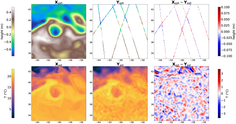
Figure 1: Images of the Ground Truth variables from GLORYS and the simulated satellite observations. The first row is the SSH variable, where the second row is the SST. The first column is the ground truth from GLORYS simulation, the second column is their associated satellite observation and the last is the difference.

2.2.3 SST observations

SST remote sensing is based on direct infrared measurements, leading to wider measurement swaths but making the measurement sensible to cloud cover. The so-called L3 satellite products have much higher data coverage, but no observation is possible when the cloud is too thick. To fill the gaps, the L3 products from several satellites are merged and interpolated to form the fully gridded image. This results in various resolutions in the same product, where high-resolution structures are artificially smoothed when the cloud coverage is too thick. To simulate this process, we use the mask of NRT L3 product [CMEMS (2023)] to retrieve a realistic cloud cover mask $C$ (between 0 and 1) which we grid to the target resolution. The SST observation operator $\mathcal{H}^{sst}$ can then be written as:

$$\mathbf{Y}^{sst}=\mathcal{H}^{sst}\left(\mathbf{X}^{sst},C\right)=(1-C)\odot\left(\mathbf{X}^{sst}+\varepsilon\right)+C\odot\mathcal{G}_{\sigma}\star\left(\mathbf{X}^{sst}+\varepsilon\right)$$ (4)

where $\odot$ is the element-wise product, $\star$ the convolution product, $\varepsilon$ is a white Gaussian noise image of size $32\times 32$ linearly upsampled to a $128\times 128$ image. We also use a spatial Gaussian filter ($\mathcal{G}_{0,\sigma}$) with $\sigma=16$(km)) to simulate the smoothing of the interpolation performed by satellite products. Our SST observations thus present a spatially and temporally correlated noise, with different resolutions depending on cloud coverage. In the end, $\mathcal{H}^{sst}$ adds a noise with a standard deviation of 0.5 °C where the SST standard deviation of the ground truth is 4.96 °C. This observation operator is different from real-world degradations but produces an image with an in-equal noise resolution similar to the errors present in the L4 SST products.

3 Proposed interpolation method

3.1 Learning the interpolation

The observation operator $\mathcal{H}^{ssh}$ previously described can be seen as a forward operator that we aim to inverse. In the past years, deep neural networks, and especially convolutional neural networks, have proven their ability to solve ill-posed image inverse problems [McCann . (2017)] and more specifically inpainting problems [Jam . (2021), Qin . (2021)]. A neural network $f_{\theta}$ is trained on a database to estimate the true state from observations $f_{\theta}(y)=\hat{x}$. Learning this inversion operator thus requires $(y,x)$ pairs (supervised) or only $y$ (unsupervised) [Ongie . (2020)].

We chose to perform the interpolation on a time window of 21 days, the input is thus a tensor of 21 images of SSH, with or without SST images, and the output is the 21 corresponding days of SSH only. An overview of the inputs and outputs of our method is provided in Figure 3. The neural network estimates the true state from observations, $\mathbf{\hat{X}}^{ssh}=f_{\theta}\left(\mathbf{Y}\right)$, where $\mathbf{Y}=\mathbf{Y}^{ssh}$ for a SSH-only interpolation, and $\mathbf{Y}=\left(\mathbf{Y}^{ssh},\mathbf{Y}^{sst}\right)$ if the network uses SST. The length of the time window will be discussed in Section 4.1, and training losses of the network in Section 3.3.

3.2 Architecture

We propose an attention-based encoder-decoder (abed) presented in Figure 2 to perform the interpolation over the time window. The attention mechanism allows to emphasize important features while neglecting irrelevant ones which makes it well-suited to extract information from contextual variables. It is widely used in many computer vision tasks [Guo . (2021)] and can be transposed to geoscience applications. The overall structure of our neural network is inspired by the one used by che2022 that introduced a residual Unet with attention layers for rain nowcasting.

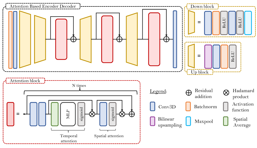
Figure 2: The architecture of the proposed Attention-Based Encoder Decoder (abed) neural network. It is designed to take a time series of 21 images of SSH, with or without a time series of SST. The encoder divides the spatial dimensions of the images by 4 through 2 “down-block”. Then the decoder uses an attention block to highlight relevant information in the images and progressively upscales it.

The encoder starts with a batch normalization and a 3D convolution (in time and in the two spatial dimensions) followed by two downsampling blocks that divide spatial dimensions by 2 (see Figure 2). The decoder is composed of residual attention blocks followed by upsampling blocks.

We describe hereafter our attention block which consists of two essential steps: temporal attention and spatial attention. Our approach builds upon the Convolutional Block Attention Module (CBAM) principle introduced by woo2018, which successively performs channel and spatial attention. We extend this idea by incorporating temporal information in the channel attention mechanism. To do so, we first compute the spatial average of each channel and instant, resulting in a tensor of size $C\times T$ where $C$ is the channel number and $T$ is the time series length. Subsequently, we apply two one-dimensional convolutional layers with a kernel of size 1, followed by a sigmoid activation function to estimate the attention weights. This corresponds to a 2-layer perceptron shared by every time step, which is different from the CBAM, as it includes the temporal information in the channel attention. These weights are then multiplied to each timestep of every channel, enabling the network to highlight salient features and suppress irrelevant information. After performing temporal attention, we proceed with spatial attention. This step involves utilizing a 3-dimensional convolutional operation, where the temporal length of the kernel size matches the length of the time series. As a result, the entire time series is aggregated into a single 2D image, which serves as the basis for deriving spatial attention. A residual skip connection is then applied, and the described block is repeated 4, 2, and 1 time for the first, second, and last block respectively. For further details about our implementation, we provide the PyTorch implementation of our network in https://gitlab.lip6.fr/archambault/james_2023.

3.3 Loss and regularization

We propose to compare two main strategies to train the neural network. Thanks to the OSSE previously described, we have access to the ground truth which we can use to learn the interpolation in a classic supervised fashion. However, it is also possible to train directly on observations, by applying the observation operator $\mathcal{H}^{ssh}$ on the generated map $\mathbf{\hat{X}}^{ssh}$ before computing the loss (see Equations 5,6,7). filoche2022 performed the interpolation with SSH observations only, and, using the same principle, archambault2023visapp showed that it was possible to overfit SSH images starting from SST only and constraining on SSH observations. Both these methods are fitted on one (or a small number) of examples and must therefore be refitted in order to be applied to unseen data. Using a larger real-world satellite dataset, martin2023 trained a neural network directly from observations, by constraining it on independent satellite observations that were not given in the input. However, the lack of ground truth reference makes it harder to compare the different reconstructions, especially regarding detected eddies and structures. We propose to train neural networks using the 3 following losses:

• The MSE using ground truth :

  $$\mathcal{L}(\mathbf{X}^{ssh},\mathbf{\hat{X}}^{ssh})=\dfrac{1}{T\times H\times W}\displaystyle\sum_{t,x,y}\left(\mathbf{X}_{t,x,y}^{ssh}-\mathbf{\hat{X}}_{t,x,y}^{ssh}\right)^{2}$$ (5)

• The MSE using only observations:

  $$\mathcal{L}_{trili}(\mathbf{Y}^{ssh},\mathbf{\hat{X}}^{ssh})=\frac{1}{N}\displaystyle\sum_{i}\left(\mathbf{Y}_{i}^{ssh}-\mathcal{H}^{ssh}(\mathbf{\hat{X}}^{ssh})_{i}\right)^{2}$$ (6)

• The MSE using only observations and the regularization introduced by martin2023:

$$\begin{split}\mathcal{L}_{trili\_reg}(\mathbf{Y}^{ssh},\mathbf{\hat{X}}^{ssh})=&\mathcal{L}_{trili}(\mathbf{Y}^{ssh},\mathbf{\hat{X}}^{ssh})+\lambda_{1}\frac{1}{N_{1}}\displaystyle\sum_{i}\left(\frac{\partial}{\partial s}\mathbf{Y}_{i}^{ssh}-\frac{\partial}{\partial s}\mathcal{H}^{ssh}(\mathbf{\hat{X}}^{ssh})_{i}\right)^{2}\\ &+\lambda_{2}\frac{1}{N_{2}}\displaystyle\sum_{i}\left(\frac{\partial^{2}}{\partial s^{2}}\mathbf{Y}_{i}^{ssh}-\frac{\partial^{2}}{\partial s^{2}}\mathcal{H}^{ssh}(\mathbf{\hat{X}}^{ssh})_{i}\right)^{2}\end{split}$$ (7)

where $\frac{\partial}{\partial s}$ is the along-track derivation of the SSH approximated by its rate of change (see Appendix 6.1). $T$ is the temporal length of the time series (here 21), $H$ and $W$ the spatial dimensions of the images (here both equals 128), and $N$, $N_{1}$, $N_{2}$, the number of satellite measures of SSH, and SSH first and second along-track spatial derivative respectively. We take $\lambda_{1}=\lambda_{2}=0.05$ the regularization coefficients, the same values used by martin2023.

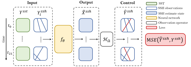
Figure 3: Computational graph of the proposed unsupervised interpolation method. The input of the neural network is a 21-day time series of SSH satellite observations, excluding data from a single satellite, and optionally includes SST measurements. The network estimates a time series of SSH fields states, upon which the observation operator is subsequently applied in order to deduce $\mathbf{\hat{Y}}^{ssh}$. Finally the Mean Squared Error between the $\mathbf{\hat{Y}}^{ssh}$ and $\mathbf{Y}^{ssh}$ is used to control the network.

The losses $\mathcal{L}_{trili}$ and $\mathcal{L}_{trili\_reg}$ apply the observation operator $\mathcal{H}^{ssh}$, before computing the MSE, which allows the training in a framework where only observations are available. Thus, from an interpolation point of view, the inversion methods that use these losses are unsupervised as they can be trained without any ground truth image. However, if we constrain the network on the same observations that were given in input, an over-fitting of along tracks will occur with no guarantee of generalization. To avoid this problem, we remove the measure from one satellite from the input of the network but calculate the loss function on all satellite observations. Doing so, the network must generalize outside the along-track measure that was given as input. In Figure 3 we call $\mathbf{Y}_{i}^{ssh}$ the input observations and present an unsupervised inversion computational graph.

3.4 Training details

Train, validation, test split. We partitioned the dataset into three subsets: training, validation, and test data. We used the year 2017 exclusively for testing our reconstructions (every analysis conducted in the following was performed on this data). We validate our methods on three distinct time intervals: (1) from July 14, 2002, to July 28, 2003, (2) from January 5, 2008, to January 18, 2009, and (3) from June 28, 2013, to July 13, 2014. The remaining data was used for training, with the exception of a 15-day period set aside to prevent data leakage.

Normalization. We normalize both the input and output of the artificial network. This involves subtracting the mean and dividing by the standard deviation, which are both computed on the entire training dataset. Specifically, for images related to SSH measurements along tracks, we first perform this normalization and subsequently replace any missing values with zeros. We normalize the neural network SSH outputs with the statistics computed on the input observations (in order that the method remains applicable in an unsupervised setting).

Training hyperparameters. We train every method using an ADAM optimizer [Kingma  Ba (2017)] with a learning rate starting at $5.10^{-5}$ and a decay of $0.99$. We perform an early stopping with a patience of 8 epochs. For the supervised training the stopping criteria is the RMSE of the reconstruction on the fully gridded domain on the validation data, but in the unsupervised setting, we compute this RMSE on left-aside along-track measures. Doing so, the stopping strategy is still compliant with a situation where no ground truth is accessible.

Ensemble. As neural network optimization is sensible to its weight initialization, we train 3 networks for every setting. The so-called “Ensemble” estimation is the average SSH map of the 3 networks. Performing an ensemble estimation helps to stabilize performances, and even enhance the reconstruction [Hinton  Dean (2015)]. In the following, we call “Ensemble score” the score of the previously mentioned ensemble estimation, and “Mean score” the average of the score of each network taken independently.

4 Results

In the following, we present the scores of the different reconstruction methods on the test set. In contrast to the training and validation method, we assess the quality of the reconstruction on the gridded ground truth. We compare the fields estimated by the 3 losses $\mathcal{L}$, $\mathcal{L}_{tri}$ and $\mathcal{L}_{tri\_reg}$ on 3 different sets of input data: one with only SSH tracks, one with SSH and the noised SST denoted nSST, and one with the noise-free SST of the GLORYS assimilation. We train interpolation methods on noise-free SST to provide an upper-bound performance of the neural network in the case of a perfect physical link between SSH and SST.

4.1 SSH reconstruction and quality of derived geostrophic currents

We give the RMSE of the SSH estimates fields in Table 1, and the RMSE on the velocity fields in Table 2. As expected, the supervised loss function outperforms the unsupervised framework in every data scenario. Specifically, in the SSH+SST scenario, the supervised loss decreases the RMSE of $\mathcal{L}_{tri}$ by 24%, and 8% without SST. Also, adding SST as an additional input to the network generally leads to improved performance compared to using SSH alone. This improvement is observed across all three loss functions, as the error values decrease for SSH+nSST compared to SSH. For instance, the SSH-only RMSE is decreased by 30% and 23% for SST and nSST respectively with $\mathcal{L}$. The regularization introduced by [SA. Martin . (2023)] slightly increases reconstruction but is still close to the unregularized inversion.

We estimate the surface currents from the reconstructed SSH from Equation 1, and we compare it to the surface circulation of the model. The errors on velocity in Table 2 follow the same patterns as the RMSE on the SSH fields but with lesser differences between methods. The RMSE is not too far from the minimal error achievable through geostrophy, which is 6.57 $\nicefrac{{cm}}{{s}}$ for $u$ and 6.14 for $v$ on this data.

Loss	SSH	SSH+nSST	SSH+SST
$\mathcal{L}$ (supervised)	4.18 — 3.85	3.23 — 2.93	2.92 — 2.59
$\mathcal{L}_{tri}$	4.52 — 4.16	3.86 — 3.51	3.62 — 3.24
$\mathcal{L}_{tri\_reg}$	4.38 — 4.13	3.73 — 3.48	3.48 — 3.20

Table 1: SSH reconstruction RMSE in centimeters (mean score on the left and ensemble score on the right) of 3 ABED networks. The interpolation is trained using the 3 different losses described in Section 3.3 with the following settings: SSH-only interpolation, SSH and noised SST, and SSH and noise-free SST. All metrics are given on the central image of a 21-day time window.

Loss	SSH		SSH+nSST		SSH+SST
	$u$	$v$	$u$	$v$	$u$	$v$
$\mathcal{L}^{*}$	13.0	14.1	10.9	11.7	10.1	10.6
$\mathcal{L}_{tri}$	13.3	15.7	12.1	14.2	11.3	13.4
$\mathcal{L}_{tri\_reg}$	12.9	14.3	11.8	12.9	11.1	12.1
*supervised

Table 2: Eastward ($u$) and northward ($v$) surface currents in cm/s. The currents were estimated by applying the geostrophy approximation (see Equation1) on the SSH ensemble estimation of the 3 ABED networks.

In Figure 4, we show the daily errors of the different methods on the test year. We notice a strong temporal variability of the RMSE with a notable increase over late Summer. Specifically, in August and September, all methods are performing worse than in Winter which can be explained by the high energy of the Ocean at this period.

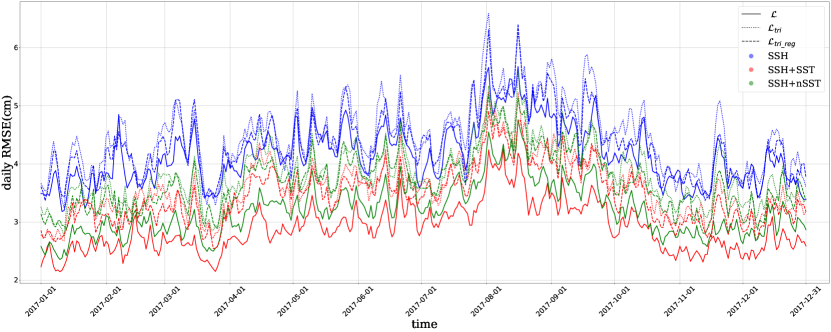
Figure 4: RMSE of the different reconstructions during the test year (2017)

An important challenge of ocean satellite products is providing real-time estimations, as many applications cannot use products available with too much time delay. In an operational framework, products that are immediately available are called Near Real Time (NRT) whereas those that require a time delay before release are called Delayed Time (DT). While in Table 1 we presented the results obtained on the central image of the time window, we can also display their scores along the 21-days temporal window as in Figure 5. The central image is a 10-day Delayed Time reconstruction as we need images of observations 10 days in the future. In Figure 5 we can verify that 21 days of data contain enough information to reconstruct the central image: for instance, 5 days from the border of the temporal window the reconstruction error is just 3% higher than the one at the center. This means that we can significantly reduce the delay (and therefore the training cost of our model) without causing severe drops in performance, which could be useful if applied in an operational framework. However, when it comes to producing NRT products (0 delay) this graph shows that we expect a significant loss of quality in the reconstruction which is usual [Amores . (2018), Stegner . (2021)]. To accurately produce an NRT image and even forecast, different training methods should be tested such as centering the target time window in the future compared to observations.

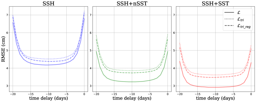
Figure 5: RMSE of the different reconstructions along the time window. The errors at a time delay of $-20$ correspond to an anti-causal scheme (knowing only future observations) whereas $timedelay=0$ corresponds to a causal scheme (knowing no future observations). Knowing both past and future observations leads to the optimal reconstruction at $timedelay=-10$.

4.2 Eddy detection analysis

4.2.1 Importance of mesoscale eddies

Mesoscale eddies play an important role in ocean circulation and dynamics and their understanding leads to diverse applications in oceanography or navigation [Chelton, Schlax  Samelson (2011)]. Previous studies underline how these structures transport heat, especially between latitudes 0° and 40° in the North Atlantic [Jayne  Marotzke (2002)], but also salinity [Amores . (2017)], or plankton [Chelton, Gaube . (2011)]. In practice, mesoscale eddies and structures are estimated through geostrophic currents derived from satellite altimetry. However, operational satellite products such as duacs, have too coarse resolutions to resolve accurately mesoscale structures. Performing an OSSE to simulate the satellite’s remote sensing amores2018,stegner2021 showed that duacs-like optimal interpolation aggregates small eddies into larger ones (i.e. with a radius greater than 100 km). These interpolations also capture a small percentage of eddies present in the model simulation (around 6% in the North Atlantic) and change the eddies’ distribution and properties. This is why we are interested in finding to what extent our reconstruction methods are able to detect small eddies in the ground truth, and how well the detected eddies are resolved and their physical properties conserved.

4.2.2 Automatic eddy detection algorithm: AMEDA

We use the Angular Momentum for Eddy Detection and tracking Algorithm (AMEDA) introduced by [Vu . (2018)] to perform the eddies detection. It is based on the Local Normalized Angular Momentum (LNAM), a dynamic metric first introduced by [Mkhinini . (2014)], that we define hereafter:

$$LNAM(P_{i})=\frac{\sum_{j}\overrightarrow{P_{i}P_{j}}\times\overrightarrow{V_{j}}}{\sum_{j}\overrightarrow{P_{i}P_{j}}.\overrightarrow{V_{j}}+\sum_{j}|\overrightarrow{P_{i}P_{j}}||\overrightarrow{V_{j}}|}=\frac{L_{i}}{S_{i}+BL_{i}}$$ (8)

where $P_{i}$ is the point of the grid where we compute the LNAM, $P_{j}$ is a neighbor point of the grid, $\overrightarrow{P_{i}P_{j}}$ is the position vector from $P_{i}$ to $P_{j}$ and $\overrightarrow{V_{j}}$ is the velocity vector in $P_{j}$. Thus, the unnormalized angular momentum $L_{i}$ is computed through a sum of cross products and is bounded by $BL_{i}$, so that if $P_{i}$ is the center of an axisymmetric cyclone (resp anticyclone), $LNAM(P_{i})$ will be equal to 1 (resp -1). Also, if the circulation field is hyperbolic and not an ellipsoid, $S_{i}$ will reach large values, and $LNAM(P_{i})$ will be close to 0. All sum is computed on a local neighborhood of $P_{i}$, which is a hyperparameter of the method (typically a square centered in $P_{i}$).

AMEDA finds potential eddy centers by searching for the local extrema of the $LNAM$ field. The shapes of the eddies are then defined by following closed current streamlines (either taking the last closed streamline, or the maximum velocity one). We perform the AMEDA algorithm on the geostrophic velocity field of our estimation and on the ground truth currents. An eddy is said to be detected if its ground truth barycenter is inside the closed streamline of its estimation.

4.2.3 Eddy detection performances

We present hereafter the detection scores of the different reconstruction methods, with three data scenarios and three losses. We take the ensemble SSH estimation of the neural networks and perform the AMEDA algorithm on the velocity field derived through the geostrophic approximation (see Equation 1).

In Table 3 we present the $F_{1}$ score, the recall, and the precision of the methods. The recall tells us the proportion of actual positive instances that were correctly identified by the detection (a recall of $1$ means that all ground truth eddies were detected). The precision measures the trust that we can put in the detected eddies (a precision of $1$ means that all eddies in the simulation were also present in the ground truth). To aggregate the recall and the precision, we use the $F_{1}$ score which is the harmonic mean of recall and precision.A value of $1$ means a perfect detection: all ground truth eddies were detected and the estimation produced no false positive.

Loss	SSH			SSH+nSST			SSH+SST
	$F_{1}$	recall	precision	$F_{1}$	recall	precision	$F_{1}$	recall	precision
$\mathcal{L}$ (supervised)	0.719	0.617	0.86	0.765	0.685	0.866	0.785	0.728	0.852
$\mathcal{L}_{tri}$	0.704	0.647	0.771	0.727	0.672	0.79	0.739	0.692	0.793
$\mathcal{L}_{tri\_reg}$	0.714	0.609	0.863	0.725	0.623	0.865	0.742	0.644	0.877

Table 3: Scores of the AMEDA eddy detection performed on the Ensemble estimation of abed interpolation. The considered scores are the precision, the recall, and the $F1$ score.

Data comparison. As expected, no matter which loss we consider, the detection method using noise-free temperature outperforms the two other scenarios with higher $F_{1}$ scores. Even the noisy SST provides important information for eddy reconstruction as the SSH-only method yields lower results than the two other scenarios. We also see that for each loss, the precision scores are less impacted by the input data than the recall is. This means that the SSH-only scenario does not produce a lot more false detection than the SST methods, but misses much more structures.

Loss comparison. On the other hand, the loss function used to perform the inversion has a substantial impact on precision and recall. The regularization of the unsupervised loss brings the detection precision to the level of the supervised method (even higher for the SSH-only and SSH+SST) but also reduces the recall of all methods compared to their unregularized version. In other words, adding a smoothness constraint on the SSH gradient field prevents the neural network from generating false eddies, but also prevents it from retrieving some structures.

4.2.4 Physical properties of detected eddies

In order to further investigate the performance of the eddy detection methods, we analyze the detection outcomes based on the physical characteristics of the eddies. For instance, smaller eddies tend to have shorter lifespans, making them more challenging to detect due to their decreased likelihood of being observed by satellites. Conversely, high-speed eddies are derived from important sea surface height (SSH) variations, thus exhibiting a strong signature in the generated mapping. Figure 6 shows the detection performances as a function of some key parameters such as the maximum radius, lifetime, or maximum velocity along the final closed current line.

As anticipated, using SST and nSST data contributes to the detection of eddies, as indicated by the higher $F_{1}$ scores achieved in every loss scenario. However, small and short-lived eddies are less frequently detected, resulting in lower recall scores. Specifically, only 17% of the eddies with a radius below 15 km are successfully detected in the best scenario. Nonetheless, except for the unregularized trilinear loss function, the precision scores for the detected eddies remain high, even for small and short-lived ones. This observation confirms the previously observed phenomenon where the regularization employed in the inversion process prevents the network from generating false eddy detections, but also stops it from capturing a significant portion of the actual eddies. This regularization behavior is expected, as forcing a smoothness constraint on the SSH gradient field leads to denying some of the small structures.

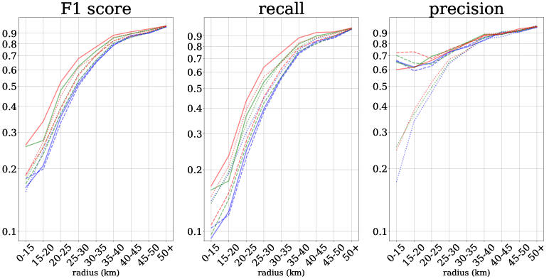
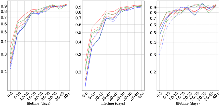
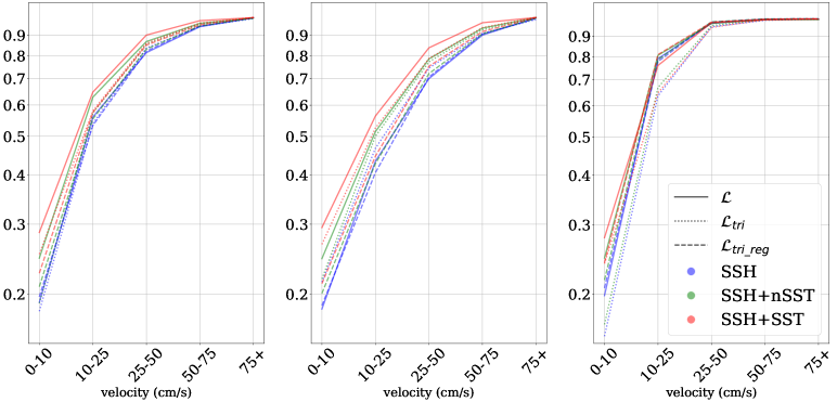
Figure 6: Detection scores of the different methods on eddies separated by radius (first row), lifetime (second row), and maximum velocity (last row). The considered scores are $F_{1}$ (first column), recall (second column), and precision (third column). The recall tells the proportion of actual positive instances that were correctly identified, the precision measures the trust that we can put in the detected eddies, and the $F_{1}$ score aggregates these two values.

We also want to assess the accuracy of the model to estimate the physical properties of the eddies. To this end, we focus on the eddies that were successfully detected by all the methods (4881 eddies out of the 7908 eddies in the ground truth). We compare the physical parameters of the estimated eddies to their values in the corresponding true eddy. To do so, we compute the RMSE and bias of the following parameters: the maximum radius and velocity, and the average distance between the centers of estimate and true eddies. The error RMSE tells us if the eddies are well resolved, whereas the bias (estimate parameter minus ground truth parameter) tells us if the interpolation method has a global tendency to overestimate or underestimate some characteristics of the eddies.

Loss	SSH		SSH+nSST		SSH+SST
	RMSE	bias	RMSE	bias	RMSE	bias
$\mathcal{L}$ (supervised)	21.8	3.8	20.5	4.5	19.0	3.8
$\mathcal{L}_{tri}$	21.5	1.6	20.4	2.2	20.8	1.7
$\mathcal{L}_{tri\_reg}$	22.4	2.9	21.7	3.3	21.2	3.9

Table 4: Eddies maximum radius RMSE and bias (km). The eddy detection is performed on geostrophic currents of the ensemble estimation and the bias is computed from the estimated radius minus ground truth radius

Loss	SSH		SSH+nSST		SSH+SST
	RMSE	bias	RMSE	bias	RMSE	bias
$\mathcal{L}$ (supervised)	12.9	-6.2	11.0	-3.8	10.2	-2.4
$\mathcal{L}_{tri}$	12.7	-5.3	11.9	-4.5	12.2	-3.8
$\mathcal{L}_{tri\_reg}$	13.8	-8.0	13.0	-6.9	12.1	-5.8

Table 5: Eddies maximum velocity RMSE and bias (cm/s)

Loss	SSH	SSH+nSST	SSH+SST
	RMSE	RMSE	RMSE
$\mathcal{L}$ (supervised)	23.2	21.7	20.3
$\mathcal{L}_{tri}$	24.5	23.5	22.9
$\mathcal{L}_{tri\_reg}$	23.4	23.2	22.2

Table 6: Eddies center position RMSE (km)

Once again, Tables 6, 6 and 6 show that SST helps to estimate eddies radius, velocity, and position. Nonetheless, there is a bias of radius and velocity: the size of the eddy is statistically overestimated compared to its ground truth, while its speed is systematically underestimated. This is particularly true for the regularized unsupervised loss because of its smoothness constraint, with a velocity bias accountable for half of the RMSE. It could be interesting to know if the estimated eddies could be unbiased without decreasing the other performances.

4.3 Comparison with state-of-the-art methods on a NATL60 OSSE

We are interested in comparing our estimations to state-of-the-art methods for gridding SSH maps. To this end, the Ocean Data Challenge 2020 [CLS/MEOM (2020)] provides a similar OSSE to the one we used, as well as the interpolations of several methods. The studied area is the same, and the included data are SSH, SST, surface currents and the simulated along tracks measures. However, the ground truth used is the NATL60 simulation [Ajayi . (2019)] which uses the same physical model (NEMO 3.6) [Madec . (2017)] but at finer scales than GLORYS, and without assimilation. Also, this simulation was run for only one year, which makes it difficult to train neural networks, this is why we designed our own OSSE. The state-of-the-art framework presented in this challenge is the following:

• duacs: the operational linear optimal interpolation leveraging covariance matrix tuned on 25 years of data.

• dymost [Ubelmann . (2016), Ballarotta . (2020)] and miost [Ardhuin . (2020)] : two variants of the linear optimal interpolation where the Gaussian covariance model is changed for a non linear surface quasi-geostrophic dynamic model (for dymost) or by a wavelet base (miost).

• bfn [Le Guillou . (2020)] : a data assimilation method that performs a back and forward nudging of a surface quasi-geostrophic model.

• 4dvarnet [Fablet . (2021)]: introduced 4dvarnet, a supervised deep learning framework. In this configuration, it only takes SSH observations as input.

• musti [Archambault . (2023)]: an unsupervised neural network that overfits SSH along tracks observations starting from an SST image. But this method must be refitted to new observations.

To produce our own estimation, we regrid the provided data to our resolution and perform the interpolation on this dataset without any finetuning or retraining. We evaluate all methods on 42 days of simulation, (between October 22nd and December 2nd 2012) which was the test set defined by the challenge. Each method is then evaluated using the following metrics, and we sum up the results in Table 7:

• $\mu$ and $\sigma_{t}$ (in cm), are respectively the RMSE of the SSH and the temporal standard deviation of this RMSE.

• $\lambda_{x}$ (in degrees) and $\lambda_{t}$ (in days) are two spectral metrics, introduced by [Le Guillou . (2020)]. We compute respectively the spatial and temporal power spectrum of the error, $\lambda_{x}$ is then the smallest spatial wavelength where the power spectrum of the error is equal to the power spectrum of the signal and $\lambda_{t}$ its temporal equivalent. For further information, we refer the reader to [Le Guillou . (2020)]

• $\mu_{u}$ and $\mu_{v}$ (in cm/s) are the RMSE between the geostrophic currents of the ground truth and the one of the estimation.

Method	SST	SUP	$\mu$	$\sigma_{t}$	$\lambda_{x}$	$\lambda_{t}$	$\mu_{u}$	$\mu_{v}$
duacs	✗	✗	4.89	3.02	1.42	12.08	16.8	16.2
dymost	✗	✗	5.18	3.05	1.35	11.87	16.8	16.8
miost	✗	✗	4.21	2.5	1.34	10.34	14.9	14.5
bfn	✗	✗	4.7	2.73	1.23	10.64	15.1	15.3
4dvarnet	✗	✓	3.26	1.73	0.84	7.95	13.1	12.8
musti	✓	✗	3.12	1.32	1.23	4.14	12.2	14.2
SSH $\mathcal{L}$	✗	✓	3.75	2.0	1.21	8.74	13.3	13.5
SSH $\mathcal{L}_{tri}$	✗	✗	4.06	2.19	1.32	9.29	13.7	15.1
SSH $\mathcal{L}_{tri\_reg}$	✗	✗	4.23	2.36	1.24	9.98	13.8	14.2
SSH+SST $\mathcal{L}$	✓	✓	2.88	1.24	0.95	4.51	11.4	11.4
SSH+SST $\mathcal{L}_{tri}$	✓	✗	3.08	1.41	1.18	5.18	11.8	12.8
SSH+SST $\mathcal{L}_{tri\_reg}$	✓	✗	3.39	1.65	1.18	5.7	12.4	12.3

Table 7: Comparison of the state-of-the-art reconstruction methods on a 43-day OSSE. SST stands for whether or not the reconstruction methods are using SST, and SUP stands for whether or not the methods are supervised.

We clearly see in thes scores a predominance of neural network-based methods (musti, 4dvarnet and ours) as the importance of the SST in the reconstruction (musti, and ours). This analysis highlights the interest in using deep learning-based methods for these inverse problems, as we can expect around 2 cm of error reduction on the operational interpolation scheme duacs with our best method (41% of reduction). We also significantly reduce the errors on currents compared to duacs’s, by 5.7 $\nicefrac{{cm}}{{s}}$ for $u$ and 5.4 $\nicefrac{{cm}}{{s}}$ for $v$ (35% and 34% error reduction).

5 Conclusion and perspectives

5.1 Summary

Throughout this study, we show promising results for a neural interpolation of SSH tracks, even while training without fully gridded data. Leveraging an Observing System Simulation Experiment, we trained an attention-based auto-encoder neural network, with 3 different loss functions (2 of them learning the reconstruction without ground truth), and using 3 sets of data (SSH only, SSH and noised SST, SSH, and SST). We show a systematic improvement of the interpolation thanks to the use of SST as well for the SSH itself, but also for the reconstruction of currents and the detection of eddies. Using temperature data (noisy or not), the unsupervised inversion outperforms even the supervised SSH-only neural network (3.86 cm of RMSE for the unsupervised noisy SST against 4.18 cm for the supervised SSH-only method). This shows the importance of contextual information to constrain the inverse problem, even while learning with observation only.

Using AMEDA, an automatic eddy detection algorithm, we were able to identify cyclones and anticyclones in the ground truth and compare them with the eddies detected in the geostrophic approximation of the different mappings. This allows a deeper physical interpretation than the SSH reconstruction alone. We conclude that SST aids in capturing finer structures that might be overlooked by SSH-only methods, but also that the key physical properties of the detected eddies such as size, speed, or center position are better rendered by SST-using methods. Furthermore, when it comes to unsupervised reconstruction, we show that the non-regularized and regularized inversions have close detection scores, but their errors are different. The regularized inversions exhibited lower recall scores, indicating that certain eddies were not detected due to the regularization process. However, they demonstrated higher precision scores, implying increased confidence in the eddies that were successfully detected.

We conducted an evaluation of our model’s performance by comparing it with state-of-the-art interpolation techniques produced during the Ocean Data Challenge 2020 which provided diverse input data, ground truth measurements, and mappings derived from different methods. Remarkably, our approach exhibits superior performance even without retraining the neural network on this novel dataset, thanks to the integration of SST information. Notably, the utilization of SST led to a substantial enhancement of 41% in terms of RMSE for SSH when compared to the widely used L4 product from duacs. Moreover, we observed significant improvements of 34% and 35% for $u$ and $v$ currents, respectively. These findings present promising perspectives for advancing satellite SSH gridding through the application of deep learning methodologies and the fusion of diverse physical information.

5.2 Perspectives

Transfer to real-world data. In this work, we performed SSH interpolation on an OSSE, which allows us to evaluate our methods on an idealized simulation of satellite tracks. The OSSE has the advantage of being more interpretable than real-world data, as the ground truth is accessible for performance evaluation, but is less realistic, especially in the simulation of SST noise which is hard to model. While simulations provide valuable insights, their direct application to real-world observations can be challenging due to inherent differences between the two domains. However, by employing transfer learning, we expect to leverage the knowledge gained from simulations to enhance reconstruction algorithms for real-world data. In further work, we are interested in comparing strategies able to learn directly from observations such as [Archambault . (2023), SA. Martin . (2023)], and a network that would benefit from supervised pre-training on simulation, and transfer on real-world observations. For instance, a model supervised on a simulation can be adapted to the new domain using one of the unsupervised losses used in this study. This will require accurate modeling of the SST input noise and an adapted transfer strategy in order for the pre-training to be efficient.

Global interpolation. Furthermore, to get toward a global gridded SSH product, many challenges still need to be addressed. For instance, as the geostrophic equilibrium depends on the Coriolis force surface projection, and thus on the latitude considered, we may require a model to be trained on several areas with different latitudes. Also, we can wonder which strategy is more efficient between training a global model or several local models, each one specialized for a range of latitude or geographical area. Closed seas and coastal water also have very different physical interactions and should be reconstructed by different methods.

Using different input and output data. We have demonstrated the benefit of using multi-physical information, specifically SST, to enhance SSH reconstruction through the implementation of a flexible neural network framework. The integration of data from diverse physical sources exhibits promising outcomes, yet conventional model-based methods encounter challenges due to noise and observational difficulties associated with real-world data. In contrast, machine learning opens doors to augment these methods with diverse and abundant data sources. For instance, in our investigation, we employed noisy yet complete SST data, but using L3 SST products is also possible. Furthermore, an intriguing prospect arises as to whether Level 4 (L4) and Level 3 (L3) SST products can be effectively combined, thereby potentially yielding even more precise and exhaustive information. Other physical measures might improve the reconstruction, such as chlorophyll maps that track plankton advected by currents [Kahru . (2012)].

Data availability statement

The GLORYS data [CMEMS (2020)] that we used as a reference throughout this study are freely available and distributed by the European Union-Copernicus Marine Service (https://doi.org/10.48670/moi-00021). The L3 altimeter [CMEMS (2021)] measures used to retrieve along tracks coordinates and the L3 SST measures[CMEMS (2023)] used to compute a realistic cloud cover are distributed by the same service (with doi https://doi.org/10.48670/MOI-00146 and https://doi.org/10.48670/MOI-00164 respectively).

The data of the Ocean Data Challenge 2020 OSSE (ground truth, inputs, and baselines) are available at https://doi.org/10.24400/527896/A01-2020.002 and were developed, validated by CLS and MEOM Team from IGE (CNRS-UGA-IRD-G-INP), France and distributed by Aviso+.

The preprocessed data and the weights of our neural networks are available here:  https://doi.org/10.5281/zenodo.8380281 and our code is hosted on the following repository: https://gitlab.lip6.fr/archambault/james_2023

6 Annexes

6.1 Along-track spatial derivative

To calculate the first and second spatial derivatives of the SSH along the ground tracks which we use to regularize the network (see Section 3.3). Given $\mathbf{Y}^{ssh}$, we approximate the derivative by the rate of change of the SSH:

$$\frac{\partial}{\partial s}\mathbf{Y}_{i}^{ssh}\simeq\frac{\mathbf{Y}_{i+1}^{ssh}-\mathbf{Y}_{i}^{ssh}}{\triangle s}$$ (9)

$$\frac{\partial^{2}}{\partial s^{2}}\mathbf{Y}_{i}^{ssh}\simeq\frac{\frac{\partial}{\partial s}\mathbf{Y}_{i+1}^{ssh}-\frac{\partial}{\partial s}\mathbf{Y}_{i}^{ssh}}{\triangle s}$$ (10)

where $\triangle s$ is the ground distance between the measures. We only compute the spatial derivatives from observations coming from the same satellite and only if the measures are taken with less than two seconds of delay. This way we estimate spatial derivatives only where the rate of change is a valid approximation of the derivation.

6.2 Detection plot

In the following, we present the Ensemble interpolation of the methods for three days. To select which day to look at, we computed the daily error of the SSH method and the SSH+SST error. The first day is chosen so that the gap between these two errors is maximal (the SST method performs a lot better than the SSH-only method). The second day corresponds to the median error gap, and the last to the minimal error gap. With the reconstructions of every method and the corresponding SSH ground truth, we also provide the SST and the noised SST. To highlight the eddy signatures in SST data we plot the ground truth eddy computed on SSH on SST images as well.

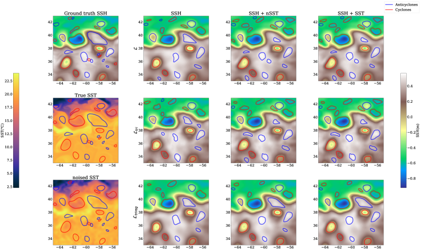
Figure 7: Eddy detection on the day of maximal error gap between SSH-only method and SST method. It corresponds to February the 7th 2017

Figure 8: Eddy detection on the day of median error gap between SSH-only method and SST method. It corresponds to December the 20th 2017

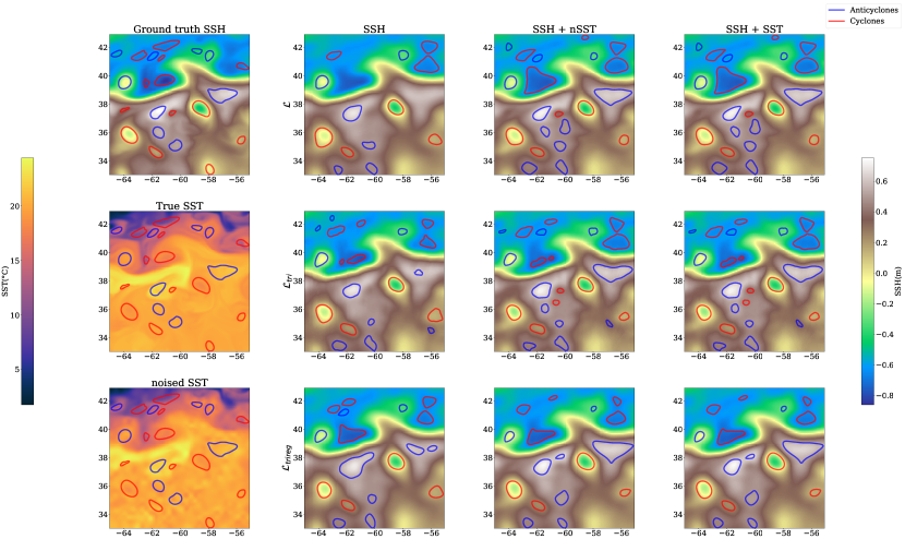
Figure 9: Eddy detection on the day of min error gap between SSH-only method and SST method. It corresponds to February the 15th 2017

References

- Ajayi \BOthers. (\APACyear2019) \APACinsertmetastarajayi2019spatial{APACrefauthors}Ajayi, A., Le Sommer, J., Chassignet, E., Molines, J\BHBIM., Xu, X., Albert, A.\BCBL \BBA Cosme, E. \APACrefYearMonthDay2019. \BBOQ\APACrefatitleSpatial and Temporal Variability of North Atlantic Eddy Field at Scale less than 100 km. Spatial and temporal variability of north atlantic eddy field at scale less than 100 km.\BBCQ \APACjournalVolNumPagesEarth and Space Science Open Archive28. {APACrefURL} https://www.essoar.org/doi/abs/10.1002/essoar.10501076.1 {APACrefDOI} 10.1002/essoar.10501076.1 \PrintBackRefs\CurrentBib
- Amores \BOthers. (\APACyear2018) \APACinsertmetastaramores2018{APACrefauthors}Amores, A., Jordà, G., Arsouze, T.\BCBL \BBA Le Sommer, J. \APACrefYearMonthDay2018\APACmonth10. \BBOQ\APACrefatitleUp to What Extent Can We Characterize Ocean Eddies Using Present-Day Gridded Altimetric Products? Up to what extent can we characterize ocean eddies using present-day gridded altimetric products?\BBCQ \APACjournalVolNumPagesJournal of Geophysical Research: Oceans1237220-7236. {APACrefDOI} 10.1029/2018JC014140 \PrintBackRefs\CurrentBib
- Amores \BOthers. (\APACyear2017) \APACinsertmetastaramores2017{APACrefauthors}Amores, A., Melnichenko, O.\BCBL \BBA Maximenko, N. \APACrefYearMonthDay20171. \BBOQ\APACrefatitleCoherent mesoscale eddies in the North Atlantic subtropical gyre: 3-D structure and transport with application to the salinity maximum Coherent mesoscale eddies in the north atlantic subtropical gyre: 3-d structure and transport with application to the salinity maximum.\BBCQ \APACjournalVolNumPagesJournal of Geophysical Research: Oceans12223-41. {APACrefDOI} 10.1002/2016JC012256 \PrintBackRefs\CurrentBib
- Archambault \BOthers. (\APACyear2023) \APACinsertmetastararchambault2023visapp{APACrefauthors}Archambault, T., Filoche, A., Charantonnis, A.\BCBL \BBA Béréziat, D. \APACrefYearMonthDay2023\APACmonth02. \BBOQ\APACrefatitleMultimodal Unsupervised Spatio-Temporal Interpolation of satellite ocean altimetry maps Multimodal Unsupervised Spatio-Temporal Interpolation of satellite ocean altimetry maps.\BBCQ \BIn \APACrefbtitleVISAPP. VISAPP. \APACaddressPublisherLisboa, Portugal. {APACrefURL} https://hal.sorbonne-universite.fr/hal-03934647 \PrintBackRefs\CurrentBib
- Ardhuin \BOthers. (\APACyear2020) \APACinsertmetastarardhuin2020_miost{APACrefauthors}Ardhuin, F., Ubelmann, C., Dibarboure, G., Gaultier, L., Ponte, A., Ballarotta, M.\BCBL \BBA Faugère, Y. \APACrefYearMonthDay202011. \APACrefbtitleReconstructing Ocean Surface Current Combining Altimetry and Future Spaceborne Doppler Data. Reconstructing ocean surface current combining altimetry and future spaceborne doppler data. \APAChowpublishedEarth and Space Science Open Archive. {APACrefURL} http://www.essoar.org/doi/10.1002/essoar.10505014.1 {APACrefDOI} 10.1002/ESSOAR.10505014.1 \PrintBackRefs\CurrentBib
- Ballarotta \BOthers. (\APACyear2020) \APACinsertmetastarballarotta2020_dymost{APACrefauthors}Ballarotta, M., Ubelmann, C., Rogé, M., Fournier, F., Faugère, Y., Dibarboure, G.\BDBLPicot, N. \APACrefYearMonthDay20209. \BBOQ\APACrefatitleDynamic Mapping of Along-Track Ocean Altimetry: Performance from Real Observations Dynamic mapping of along-track ocean altimetry: Performance from real observations.\BBCQ \APACjournalVolNumPagesJournal of Atmospheric and Oceanic Technology371593-1601. {APACrefURL} https://journals.ametsoc.org/view/journals/atot/37/9/jtechD200030.xml {APACrefDOI} 10.1175/JTECH-D-20-0030.1 \PrintBackRefs\CurrentBib
- Che \BOthers. (\APACyear2022) \APACinsertmetastarche2022{APACrefauthors}Che, H., Niu, D., Zang, Z., Cao, Y.\BCBL \BBA Chen, X. \APACrefYearMonthDay2022. \BBOQ\APACrefatitleED-DRAP: Encoder–Decoder Deep Residual Attention Prediction Network for Radar Echoes Ed-drap: Encoder–decoder deep residual attention prediction network for radar echoes.\BBCQ \APACjournalVolNumPagesIEEE Geoscience and Remote Sensing Letters19. {APACrefDOI} 10.1109/LGRS.2022.3141498 \PrintBackRefs\CurrentBib
- Chelton, Gaube\BCBL \BOthers. (\APACyear2011) \APACinsertmetastarchelton2011_chl{APACrefauthors}Chelton, D\BPBIB., Gaube, P., Schlax, M\BPBIG., Early, J\BPBIJ.\BCBL \BBA Samelson, R\BPBIM. \APACrefYearMonthDay201110. \BBOQ\APACrefatitleThe Influence of Nonlinear Mesoscale Eddies on Near-Surface Oceanic Chlorophyll The influence of nonlinear mesoscale eddies on near-surface oceanic chlorophyll.\BBCQ \APACjournalVolNumPagesScience334328-332. {APACrefDOI} 10.1126/SCIENCE.1208897 \PrintBackRefs\CurrentBib
- Chelton, Schlax\BCBL \BBA Samelson (\APACyear2011) \APACinsertmetastarchelton2011{APACrefauthors}Chelton, D\BPBIB., Schlax, M\BPBIG.\BCBL \BBA Samelson, R\BPBIM. \APACrefYearMonthDay201110. \BBOQ\APACrefatitleGlobal observations of nonlinear mesoscale eddies Global observations of nonlinear mesoscale eddies.\BBCQ \APACjournalVolNumPagesProgress in Oceanography91167-216. {APACrefDOI} 10.1016/J.POCEAN.2011.01.002 \PrintBackRefs\CurrentBib
- Ciani \BOthers. (\APACyear2020) \APACinsertmetastarciani2020{APACrefauthors}Ciani, D., Rio, M\BHBIH., Bruno Nardelli, B., Etienne, H.\BCBL \BBA Santoleri, R. \APACrefYearMonthDay2020\APACmonth05. \BBOQ\APACrefatitleImproving the Altimeter-Derived Surface Currents Using Sea Surface Temperature (SST) Data: A Sensitivity Study to SST Products Improving the altimeter-derived surface currents using sea surface temperature (SST) data: A sensitivity study to SST products.\BBCQ \APACjournalVolNumPagesRemote Sensing121601. {APACrefURL} https://www.mdpi.com/2072-4292/12/10/1601/htmhttps://www.mdpi.com/2072-4292/12/10/1601 {APACrefDOI} 10.3390/RS12101601 \PrintBackRefs\CurrentBib
- CLS/MEOM (\APACyear2020) \APACinsertmetastarDATAch2020{APACrefauthors}CLS/MEOM. \APACrefYearMonthDay2020. \APACrefbtitleSWOT Data Challenge NATL60 [Dataset]. Swot data challenge natl60 [dataset]. \APACaddressPublisherCNES. {APACrefDOI} https://doi.org/10.24400/527896/A01-2020.002 \PrintBackRefs\CurrentBib
- CMEMS (\APACyear2020) \APACinsertmetastarDATAglorys{APACrefauthors}CMEMS. \APACrefYearMonthDay2020. \APACrefbtitleGlobal Ocean Physics Reanalysis [Dataset]. Global ocean physics reanalysis [dataset]. \APACaddressPublisherMercator Ocean International. {APACrefDOI} https://doi.org/10.48670/moi-00021 \PrintBackRefs\CurrentBib
- CMEMS (\APACyear2021) \APACinsertmetastarDATAL3tracks{APACrefauthors}CMEMS. \APACrefYearMonthDay2021. \APACrefbtitleGlobal Ocean Along-Track L3 Sea Surface Heights Reprocessed (1993-Ongoing) Tailored For Data Assimilation [Dataset]. Global ocean along-track l3 sea surface heights reprocessed (1993-ongoing) tailored for data assimilation [dataset]. \APACaddressPublisherMercator Ocean International. {APACrefDOI} https://doi.org/10.48670/MOI-00146 \PrintBackRefs\CurrentBib
- CMEMS (\APACyear2023) \APACinsertmetastarDATAcloud{APACrefauthors}CMEMS. \APACrefYearMonthDay2023. \APACrefbtitleGlobal Oceans Sea Surface Temperature Multi-sensor L3 Observations [Dataset]. Global oceans sea surface temperature multi-sensor l3 observations [dataset]. \APACaddressPublisherMercator Ocean International. {APACrefDOI} https://doi.org/10.48670/MOI-00164 \PrintBackRefs\CurrentBib
- Emery \BOthers. (\APACyear1989) \APACinsertmetastaremery1989avhrr{APACrefauthors}Emery, W\BPBIJ., Brown, J.\BCBL \BBA Nowak, Z\BPBIP. \APACrefYearMonthDay1989. \BBOQ\APACrefatitleAVHRR image navigation-Summary and review AVHRR image navigation-summary and review.\BBCQ \APACjournalVolNumPagesPhotogrammetric engineering and remote sensing41175–1183. \PrintBackRefs\CurrentBib
- Fablet \BOthers. (\APACyear2021) \APACinsertmetastarfablet2021{APACrefauthors}Fablet, R., Amar, M., Febvre, Q., Beauchamp, M.\BCBL \BBA Chapron, B. \APACrefYearMonthDay2021\APACmonth06. \BBOQ\APACrefatitleEnd-to-end physics-informed representation learning for satellite ocean remote sensing data: Applications to satellite altimetry and sea surface currents End-to-end physics-informed representation learning for satellite ocean remote sensing data: Applications to satellite altimetry and sea surface currents.\BBCQ \APACjournalVolNumPagesISPRS Annals of the Photogrammetry, Remote Sensing and Spatial Information Sciences5295-302. {APACrefDOI} 10.5194/ISPRS-ANNALS-V-3-2021-295-2021 \PrintBackRefs\CurrentBib
- Fablet \BOthers. (\APACyear2023) \APACinsertmetastarfablet2023{APACrefauthors}Fablet, R., Febvre, Q.\BCBL \BBA Chapron, B. \APACrefYearMonthDay2023. \BBOQ\APACrefatitleMultimodal 4DVarNets for the Reconstruction of Sea Surface Dynamics From SST-SSH Synergies Multimodal 4dvarnets for the reconstruction of sea surface dynamics from sst-ssh synergies.\BBCQ \APACjournalVolNumPagesIEEE Transactions on Geoscience and Remote Sensing61. {APACrefDOI} 10.1109/TGRS.2023.3268006 \PrintBackRefs\CurrentBib
- Filoche \BOthers. (\APACyear2022) \APACinsertmetastarfiloche2022{APACrefauthors}Filoche, A., Archambault, T., Charantonis, A.\BCBL \BBA Béréziat, D. \APACrefYearMonthDay2022. \BBOQ\APACrefatitleStatistics-free interpolation of ocean observations with deep spatio-temporal prior Statistics-free interpolation of ocean observations with deep spatio-temporal prior.\BBCQ \BIn \APACrefbtitleECML/PKDD Workshop on Machine Learning for Earth Observation and Prediction (MACLEAN). Ecml/pkdd workshop on machine learning for earth observation and prediction (maclean). {APACrefURL} https://hal.sorbonne-universite.fr/hal-03765735 \PrintBackRefs\CurrentBib
- Gaultier \BOthers. (\APACyear2016) \APACinsertmetastargaultier2016{APACrefauthors}Gaultier, L., Ubelmann, C.\BCBL \BBA Fu, L. \APACrefYearMonthDay2016. \BBOQ\APACrefatitleThe challenge of using future SWOT data for oceanic field reconstruction The challenge of using future SWOT data for oceanic field reconstruction.\BBCQ \APACjournalVolNumPagesJournal of Atmospheric and Oceanic Technology33119-126. {APACrefDOI} 10.1175/JTECH-D-15-0160.1 \PrintBackRefs\CurrentBib
- Guo \BOthers. (\APACyear2021) \APACinsertmetastarguo2021{APACrefauthors}Guo, M\BHBIH., Xu, T\BHBIX., Liu, J\BHBIJ., Liu, Z\BHBIN., Jiang, P\BHBIT., Mu, T\BHBIJ.\BDBLHu, S\BHBIM. \APACrefYearMonthDay202111. \BBOQ\APACrefatitleAttention Mechanisms in Computer Vision: A Survey Attention mechanisms in computer vision: A survey.\BBCQ \APACjournalVolNumPagesComputational Visual Media8331-368. {APACrefURL} http://arxiv.org/abs/2111.07624http://dx.doi.org/10.1007/s41095-022-0271-y {APACrefDOI} 10.1007/s41095-022-0271-y \PrintBackRefs\CurrentBib
- Hinton \BBA Dean (\APACyear2015) \APACinsertmetastarHinton2015{APACrefauthors}Hinton, G.\BCBT \BBA Dean, J. \APACrefYearMonthDay2015. \BBOQ\APACrefatitleDistilling the Knowledge in a Neural Network Distilling the knowledge in a neural network.\BBCQ \BIn \APACrefbtitleNIPS Deep Learning and Representation Learning Workshop. Nips deep learning and representation learning workshop. \PrintBackRefs\CurrentBib
- Isern-Fontanet \BOthers. (\APACyear2006) \APACinsertmetastarisernfontanet2006{APACrefauthors}Isern-Fontanet, J., Chapron, B., Lapeyre, G.\BCBL \BBA Klein, P. \APACrefYearMonthDay2006. \BBOQ\APACrefatitlePotential use of microwave sea surface temperatures for the estimation of ocean currents Potential use of microwave sea surface temperatures for the estimation of ocean currents.\BBCQ \APACjournalVolNumPagesGeophys. Res. Lett3324608. {APACrefURL} http://www.ecco-group.org {APACrefDOI} 10.1029/2006GL027801 \PrintBackRefs\CurrentBib
- Jam \BOthers. (\APACyear2021) \APACinsertmetastarjam2021{APACrefauthors}Jam, J., Kendrick, C., Walker, K., Drouard, V., Hsu, J.\BCBL \BBA Yap, M. \APACrefYearMonthDay2021\APACmonth02. \BBOQ\APACrefatitleA comprehensive review of past and present image inpainting methods A comprehensive review of past and present image inpainting methods.\BBCQ \APACjournalVolNumPagesComputer Vision and Image Understanding203. {APACrefDOI} 10.1016/J.CVIU.2020.103147 \PrintBackRefs\CurrentBib
- Jayne \BBA Marotzke (\APACyear2002) \APACinsertmetastarjayne2002{APACrefauthors}Jayne, S.\BCBT \BBA Marotzke, J. \APACrefYearMonthDay200212. \BBOQ\APACrefatitleThe Oceanic Eddy Heat Transport The oceanic eddy heat transport.\BBCQ \APACjournalVolNumPagesJournal of Physical Oceanography323328-3345. {APACrefDOI} 10.1175/1520-0485(2002)032¡3328:TOEHT¿2.0.CO;2 \PrintBackRefs\CurrentBib
- Kahru \BOthers. (\APACyear2012) \APACinsertmetastarKahru2012{APACrefauthors}Kahru, M., Di Lorenzo, E., Manzano-Sarabia, M.\BCBL \BBA Mitchell, B\BPBIG. \APACrefYearMonthDay201203. \BBOQ\APACrefatitleSpatial and temporal statistics of sea surface temperature and chlorophyll fronts in the California Current Spatial and temporal statistics of sea surface temperature and chlorophyll fronts in the California Current.\BBCQ \APACjournalVolNumPagesJournal of Plankton Research349749-760. {APACrefURL} https://doi.org/10.1093/plankt/fbs010 {APACrefDOI} 10.1093/plankt/fbs010 \PrintBackRefs\CurrentBib
- Kingma \BBA Ba (\APACyear2017) \APACinsertmetastarkingma2017adam{APACrefauthors}Kingma, D\BPBIP.\BCBT \BBA Ba, J. \APACrefYearMonthDay2017. \APACrefbtitleAdam: A Method for Stochastic Optimization. Adam: A method for stochastic optimization. \PrintBackRefs\CurrentBib
- Le Guillou \BOthers. (\APACyear2020) \APACinsertmetastarguillou2020_bfn{APACrefauthors}Le Guillou, F., Metref, S., Cosme, E., Ubelmann, C., Ballarotta, M., Verron, J.\BCBL \BBA Le Sommer, J. \APACrefYearMonthDay202010. \APACrefbtitleMapping altimetry in the forthcoming SWOT era by back-and-forth nudging a one-layer quasi-geostrophic model. Mapping altimetry in the forthcoming SWOT era by back-and-forth nudging a one-layer quasi-geostrophic model. \APAChowpublishedEarth and Space Science Open Archive. {APACrefURL} http://www.essoar.org/doi/10.1002/essoar.10504575.1 {APACrefDOI} 10.1002/ESSOAR.10504575.1 \PrintBackRefs\CurrentBib
- Madec \BOthers. (\APACyear2017) \APACinsertmetastarmadec2017nemo{APACrefauthors}Madec, G., Bourdallé-Badie, R., Bouttier, P\BHBIA., Bricaud, C., Bruciaferri, D., Calvert, D.\BDBLothers \APACrefYearMonthDay2017. \APACrefbtitleNEMO ocean engine. Nemo ocean engine. \PrintBackRefs\CurrentBib
- S. Martin (\APACyear2014) \APACinsertmetastarmartin_2014{APACrefauthors}Martin, S. \APACrefYear2014. \APACrefbtitleAn Introduction to Ocean Remote Sensing An introduction to ocean remote sensing (\PrintOrdinal2 \BEd). \APACaddressPublisherCambridge University Press. {APACrefDOI} 10.1017/CBO9781139094368 \PrintBackRefs\CurrentBib
- S\BPBIA. Martin \BOthers. (\APACyear2023) \APACinsertmetastarmartin2023{APACrefauthors}Martin, S\BPBIA., Manucharyan, G\BPBIE.\BCBL \BBA Klein, P. \APACrefYearMonthDay2023. \BBOQ\APACrefatitleSynthesizing Sea Surface Temperature and Satellite Altimetry Observations Using Deep Learning Improves the Accuracy and Resolution of Gridded Sea Surface Height Anomalies Synthesizing sea surface temperature and satellite altimetry observations using deep learning improves the accuracy and resolution of gridded sea surface height anomalies.\BBCQ \APACjournalVolNumPagesJournal of Advances in Modeling Earth Systems155e2022MS003589. {APACrefURL} https://agupubs.onlinelibrary.wiley.com/doi/abs/10.1029/2022MS003589 \APACrefnotee2022MS003589 2022MS003589 {APACrefDOI} https://doi.org/10.1029/2022MS003589 \PrintBackRefs\CurrentBib
- McCann \BOthers. (\APACyear2017) \APACinsertmetastarmccann2017{APACrefauthors}McCann, M., Jin, K.\BCBL \BBA Unser, M. \APACrefYearMonthDay201711. \BBOQ\APACrefatitleConvolutional neural networks for inverse problems in imaging: A review Convolutional neural networks for inverse problems in imaging: A review.\BBCQ \APACjournalVolNumPagesIEEE Signal Processing Magazine3485–95. {APACrefURL} http://arxiv.org/abs/1710.04011http://dx.doi.org/10.1109/MSP.2017.2739299 {APACrefDOI} 10.1109/MSP.2017.2739299 \PrintBackRefs\CurrentBib
- Mkhinini \BOthers. (\APACyear2014) \APACinsertmetastarmkhinini2014{APACrefauthors}Mkhinini, N., Coimbra, A\BPBIL\BPBIS., Stegner, A., Arsouze, T., Taupier-Letage, I.\BCBL \BBA Béranger, K. \APACrefYearMonthDay201412. \BBOQ\APACrefatitleLong-lived mesoscale eddies in the eastern Mediterranean Sea: Analysis of 20 years of AVISO geostrophic velocities Long-lived mesoscale eddies in the eastern mediterranean sea: Analysis of 20 years of aviso geostrophic velocities.\BBCQ \APACjournalVolNumPagesJournal of Geophysical Research: Oceans1198603-8626. {APACrefURL} https://onlinelibrary.wiley.com/doi/full/10.1002/2014JC010176 {APACrefDOI} 10.1002/2014JC010176 \PrintBackRefs\CurrentBib
- Nardelli \BOthers. (\APACyear2022) \APACinsertmetastarnardelli2022{APACrefauthors}Nardelli, B., Cavaliere, D., Charles, E.\BCBL \BBA Ciani, D. \APACrefYearMonthDay2022\APACmonth02. \BBOQ\APACrefatitleSuper-Resolving Ocean Dynamics from Space with Computer Vision Algorithms Super-resolving ocean dynamics from space with computer vision algorithms.\BBCQ \APACjournalVolNumPagesRemote Sensing141159. {APACrefURL} https://www.mdpi.com/2072-4292/14/5/1159/htmhttps://www.mdpi.com/2072-4292/14/5/1159 {APACrefDOI} 10.3390/RS14051159 \PrintBackRefs\CurrentBib
- Ongie \BOthers. (\APACyear2020) \APACinsertmetastarongie2020{APACrefauthors}Ongie, O., Jalal, A., Metzler, C., Baraniuk, R., Dimakis, A.\BCBL \BBA Willett, R. \APACrefYearMonthDay2020\APACmonth05. \BBOQ\APACrefatitleDeep Learning Techniques for Inverse Problems in Imaging Deep learning techniques for inverse problems in imaging.\BBCQ \APACjournalVolNumPagesIEEE Journal on Selected Areas in Information Theory139–56. \PrintBackRefs\CurrentBib
- Qin \BOthers. (\APACyear2021) \APACinsertmetastarqin2021{APACrefauthors}Qin, Z., Zeng, Q., Zong, Y.\BCBL \BBA Xu, F. \APACrefYearMonthDay20219. \BBOQ\APACrefatitleImage inpainting based on deep learning: A review Image inpainting based on deep learning: A review.\BBCQ \APACjournalVolNumPagesDisplays69102028. {APACrefDOI} 10.1016/J.DISPLA.2021.102028 \PrintBackRefs\CurrentBib
- Stegner \BOthers. (\APACyear2021) \APACinsertmetastarstegner2021{APACrefauthors}Stegner, A., Le Vu, B., Dumas, F., Ghannami, M., Nicolle, A., Durand, C.\BCBL \BBA Faugere, Y. \APACrefYearMonthDay2021\APACmonth09. \BBOQ\APACrefatitleCyclone-Anticyclone Asymmetry of Eddy Detection on Gridded Altimetry Product in the Mediterranean Sea Cyclone-anticyclone asymmetry of eddy detection on gridded altimetry product in the mediterranean sea.\BBCQ \APACjournalVolNumPagesJournal of Geophysical Research: Oceans126. {APACrefDOI} 10.1029/2021JC017475 \PrintBackRefs\CurrentBib
- Taburet \BOthers. (\APACyear2019) \APACinsertmetastartaburet2019{APACrefauthors}Taburet, G., Sanchez-Roman, A., Ballarotta, M., Pujol, M\BHBII., Legeais, J\BHBIF., Fournier, F.\BDBLDibarboure, G. \APACrefYearMonthDay2019. \BBOQ\APACrefatitleDUACS DT2018: 25 years of reprocessed sea level altimetry products DUACS DT2018: 25 years of reprocessed sea level altimetry products.\BBCQ \APACjournalVolNumPagesOcean Sci151207-1224. {APACrefURL} https://doi.org/10.5194/os-15-1207-2019 {APACrefDOI} 10.5194/os-15-1207-2019 \PrintBackRefs\CurrentBib
- Thiria \BOthers. (\APACyear2023) \APACinsertmetastarresac{APACrefauthors}Thiria, S., Sorror, C., Archambault, T., Charantonis, A., Béréziat, D., Mejia, C.\BDBLCrepon, M. \APACrefYearMonthDay2023. \BBOQ\APACrefatitleDownscaling of ocean fields by fusion of heterogeneous observations using Deep Learning algorithms Downscaling of ocean fields by fusion of heterogeneous observations using deep learning algorithms.\BBCQ \APACjournalVolNumPagesOcean Modeling. \PrintBackRefs\CurrentBib
- Ubelmann \BOthers. (\APACyear2016) \APACinsertmetastarubelmann2016_dymost{APACrefauthors}Ubelmann, C., Cornuelle, B.\BCBL \BBA Fu, L. \APACrefYearMonthDay2016\APACmonth08. \BBOQ\APACrefatitleDynamic Mapping of Along-Track Ocean Altimetry: Method and Performance from Observing System Simulation Experiments Dynamic mapping of along-track ocean altimetry: Method and performance from observing system simulation experiments.\BBCQ \APACjournalVolNumPagesJournal of Atmospheric and Oceanic Technology331691-1699. {APACrefURL} https://journals.ametsoc.org/view/journals/atot/33/8/jtech-d-15-0163_1.xml {APACrefDOI} 10.1175/JTECH-D-15-0163.1 \PrintBackRefs\CurrentBib
- Vu \BOthers. (\APACyear2018) \APACinsertmetastarAMEDA{APACrefauthors}Vu, B\BPBIL., Stegner, A.\BCBL \BBA Arsouze, T. \APACrefYearMonthDay20184. \BBOQ\APACrefatitleAngular Momentum Eddy Detection and Tracking Algorithm (AMEDA) and Its Application to Coastal Eddy Formation Angular momentum eddy detection and tracking algorithm (ameda) and its application to coastal eddy formation.\BBCQ \APACjournalVolNumPagesJournal of Atmospheric and Oceanic Technology35739-762. {APACrefURL} https://journals.ametsoc.org/view/journals/atot/35/4/jtech-d-17-0010.1.xml {APACrefDOI} 10.1175/JTECH-D-17-0010.1 \PrintBackRefs\CurrentBib
- Woo \BOthers. (\APACyear2018) \APACinsertmetastarwoo2018{APACrefauthors}Woo, S., Park, J., Lee, J\BHBIY.\BCBL \BBA Kweon, I\BPBIS. \APACrefYearMonthDay2018. \BBOQ\APACrefatitleCBAM: Convolutional Block Attention Module Cbam: Convolutional block attention module.\BBCQ \APACjournalVolNumPagesComputer Vision and Pattern Recognition. \PrintBackRefs\CurrentBib