Prospective Side Information for Latent MDPs

Abstract

In many interactive decision-making settings, there is latent and unobserved information that remains fixed. Consider, for example, a dialogue system, where complete information about a user, such as the user’s preferences, is not given. In such an environment, the latent information remains fixed throughout each episode, since the identity of the user does not change during an interaction. This type of environment can be modeled as a Latent Markov Decision Process (LMDP), a special instance of Partially Observed Markov Decision Processes (POMDPs). Recently, Kwon et al. (2021) established exponential lower bounds in the number of latent contexts for the LMDP class. This puts forward a question: under which natural assumptions a near-optimal policy of an LMDP can be efficiently learned? In this work, we study the class of LMDPs with prospective side information, when an agent receives additional, weakly revealing, information on the latent context at the beginning of each episode. We show that, surprisingly, this problem is not captured by contemporary settings and algorithms designed for partially observed environments. We then establish that any sample efficient algorithm must suffer at least $\Omega(K^{2/3})$-regret, as opposed to standard $\Omega(\sqrt{K})$ lower bounds, and design an algorithm with a matching upper bound.

1 Introduction

Many real-world sequential decision problems are partially observed, and full information on the state of the system is not known. In its full generality, such a setting can be formulated as a Partially Observed Markov Decision Process (POMDP). Due to its prevalence, POMDPs have been extensively studied in past decades Smallwood and Sondik (1973); Pineau et al. (2006). Yet, with no further assumptions, it is known to be hard from both computational and learnability perspectives Papadimitriou and Tsitsiklis (1987); Krishnamurthy et al. (2016). A possible meaningful way moving forward is to restrict the study to special and widespread classes of POMDPs. Recent advances in literature put efforts into identifying tractable subclasses of POMDPs in several aspects Dann et al. (2018); Du et al. (2019); Efroni et al. (2022); Uehara et al. (2022); Kwon et al. (2021); Liu et al. (2022).

We consider a partially observed sequential problem in which the latent information remains fixed during each episodic interaction Chadès et al. (2012); Hallak et al. (2015); Brunskill and Li (2013); Steimle et al. (2018); Kwon et al. (2021), also referred as Latent MDPs (LMDPs). Such a setting can model many common problems, e.g., dialogue and recommender systems, when complete information on a user is not given, yet, each user remains fixed within each episodic interaction. Recently, Kwon et al. (2021, 2023) derived exponential worst-case lower bounds in the number of contexts for this subclass of POMDPs. This implies that, in general, near optimal policy of an LMDP cannot be learned efficiently when the number of latent context is large.

Under which assumptions, common in practice, do LMDPs can be efficiently learned? Prior work Kwon et al. (2021); Zhou et al. (2022); Lee et al. (2023) established that given complete information on the latent context in hindsight, i.e., at the end of each episode, LMDPs can be learned efficiently. In this work, we study a somewhat dual assumption; we assume that an agent can observe a weakly revealing side information on the latent context at the beginning of each episode, and refer it as LMDP with Prospective Side Information, or as LMDP-$\Psi$. Differently than the case information is available in hindsight, for the LMDP-$\Psi$ setting, the policy can utilize the additional hint within each episode. We study lower bounds and matching upper bounds for this class of problems, and show this setting is tractable from the sample complexity perspective.

	MDP	$\alpha$-Revealing POMDP	LMDP with $\alpha$-Prospective SI	LMDP	POMDP
UB	$\sqrt{AK}$	$\mathrm{poly}(A,\alpha^{-1})\sqrt{K}$	$\mathrm{poly}(A,\alpha^{-1})K^{2/3}$	—	$A^{H}\sqrt{K}$
LB	$\sqrt{AK}$	$\mathrm{poly}(A,\alpha^{-1})\sqrt{K}$	$\min\left(A^{\Omega(M)}\sqrt{K},\mathrm{poly}(A,\alpha^{-1})K^{2/3}\right)$	$A^{M}\sqrt{K}$	$A^{H}\sqrt{K}$

Table 1: Regret upper and lower bounds in different classes of POMDPs, ordered by their degree of difficulty from the simplest to hardest (left to right). Dependencies on other problem parameters are omitted (e.g. $S$ and $H$). The results and the setting introduced in this work are highlighted in green.

Technically speaking, our work builds upon recent algorithmic advancements for POMDPs Liu et al. (2023); Uehara et al. (2022); Huang et al. (2023). However, proper application of these requires care. As we show, the LMDP-$\Psi$ class is not contained within the class of POMDPs previously known to be efficiently learnable, and, in fact, goes beyond common POMDP modeling assumptions. Further, we highlight a surprising limitation of exploiting the prospective side information on the latent context.

Our Contributions

The main contributions of this work are the following (see also Table 1). We introduce the problem of learning a near-optimal policy with $\alpha$-prospective side information for LMDPs, when the prospective side information weakly reveals information on the true latent state. We provide a $\mathrm{poly}(A,\alpha^{-1})K^{2/3}$ regret upper bound, by building upon the pure exploration scheme developed in Huang et al. (2023). Namely, our upper bound does not suffer exponential dependence in the number of latent contexts. We also provide a lower bound of $\Omega\left(\frac{A}{\alpha^{2}\epsilon^{2}}K^{2/3}\right)$ to this problem, unlike the $K^{1/2}$ rate one may expect.

2 Preliminaries

An episodic LMDP is defined as follows:

Definition 2.1 (Latent MDP)

An LMDP instance consists of a tuple $\theta:=\left(\{p_{m}\}_{m=1}^{M},\{\mathbb{T}_{m}\}_{m=1}^{M},\{\mathbb{O}_{m}\}_{m=1}^{M}\right)$, where $M$ is the number of latent contexts; $\{p_{m}\}_{m=1}^{M}$ are the mixing weights, the probability latent context $m$ is drawn at the beginning of an episode; $\mathbb{T}_{m}\in\mathbb{R}^{S\times S\times A},\mathbb{O}_{m}\in\mathbb{R}^{|\mathcal{O}|\times S\times A}$ are the transition probabilities and instant observation distribution of $m^{th}$ MDPs, i.e., $\mathbb{T}_{m}(s^{\prime}|s,a):=\mathds{P}(s^{\prime}|m,s,a)$ and $\mathbb{O}_{m}(o,s,a):=\mathds{P}(o|m,s,a)$ for state $s\in\mathcal{S}$, next state $s^{\prime}\in\mathcal{S}$, action $a\in\mathcal{A}$, instanteneous observation $o\in\mathcal{O}$, and latent context $m\in[M]$.

We assume that for all $o\in\mathcal{O}$, there is a known reward-decoding function $r:\mathcal{O}\rightarrow\mathbb{R}$, and each reward is bounded $|r(o)|\leq 1$. To simplify the discussion, we assume that the set of LMDP instances $\Theta$ has finite (but exponentially large) cardinality $|\Theta|$. Similarly, we also assume that the observation space is discrete and finite:

Assumption 1 (Observation Space)

Each observation attains a value in the set $\mathcal{O}$ which has finite but could be arbitrarily large cardinality $|\mathcal{O}|$.

All claims made in this paper hold similarly for the continuous model class with a standard $\epsilon$-discretization of $\Theta$ with the extra discretization error analysis similar to Liu et al. (2022) and continuous observations Liu et al. (2023).

At the beginning of every episode, a latent and unobserved context $m\in[M]$ is sampled from a mixing distribution $\{p_{m}\}_{m=1}^{M}$ and is fixed for $H$ time steps. Without loss of generality, we assume that the system starts from time-step $t=0$ at a fixed initial state $s_{\text{dummy}}$ and transits to other states following the initial state distribution of the chosen MDP regardless of taken actions (and we always see a dummy observation $o_{\text{dummy}}$).

Prospective Side Information for LMDPs.

In this work, we assume the LMDP is augmented with prospective side information. Prospective side information is an additional observation given prior to the beginning of the episode and remains fixed along a trajectory. Let $\mathcal{I}$ be the set of prospective side information values, and is assumed to be finite but may be arbitrarily large. Let $\mathbb{I}\in\mathbb{R}^{|\mathcal{I}|\times M}$ be a context dependent emission matrix, i.e., $\mathbb{I}(\iota,m):=\mathds{P}(\iota|m)$. We assume that the prospective side information is given only at the beginning of each episode and remains fixed during the entire episode. Further, we assume it provides some hint on the identity of the true latent MDP. Formally, we assume the following weakly revealing condition:

Assumption 2 (Prospective Side Information)

For any two belief vectors $\bar{v}_{1},\bar{v}_{2}\in\Delta([M])$,

$$d_{\texttt{TV}}\left(\mathds{P}(\iota|\bar{v}_{1}),\mathds{P}(\iota|\bar{v}_{2})\right)\geq\frac{\alpha}{2}\|\bar{v}_{1}-\bar{v}_{2}\|_{1}.$$ (1)

With these definitions at hand, we can define the setting studied in this work. We consider the LMDP with Prospective Side Information, which we refer to as LMDP-$\Psi$, which is the tuple $\theta=(\mathbb{I},\{p_{m},\mathbb{T}_{m},\mathbb{O}_{m}\}_{m=1}^{M})\in\Theta$.

Accordingly, our goal is now to learn an $\epsilon$-optimal policy from a larger class of policies $\Pi:\mathcal{I}\times(\mathcal{A}\times\mathcal{O}\times\mathcal{S})^{*}\rightarrow\Delta(\mathcal{A})$ that exploits the prospective side information, given prior to each episodic interaction. An important subclass of this larger policy class is the side information blind policies $\Pi_{\texttt{blind}}:(\mathcal{A}\times\mathcal{O}\times\mathcal{S})^{*}\rightarrow\Delta(\mathcal{A})$, that does not exploit the prospective side information within each trajectory. As we see, the nature of the problem becomes different by the capacity of the policy class.

The optimal policy $\pi^{*}$ is defined as the optimal history-dependent policy that maximizes the expected cumulative reward

$$V^{\star}=\max_{\pi\in\Pi}V^{\pi}:=\mathbb{E}^{\pi}\left[\textstyle\sum_{t=1}^{H}r_{t}(o_{t})\right],$$

where the expectation is taken over latent contexts and rewards generated by an LMDP instance, following policy $\pi$. We let $\pi^{*}_{\texttt{blind}}$ be the counterpart in the smaller policy class $\Pi_{\texttt{blind}}$.

Notation

We occasionally use the symbol $\lesssim$ to mean that the inequality holds up to some absolute constant. We use $\lesssim_{\texttt{P}}$ when it holds up to some problem dependent polynomial factors. To simplify notation, we occasionally denote pair-wise quantities as $x_{t}:=(s_{t},a_{t})$, $y_{t}:=(o_{t},s_{t+1})$. $\mathrm{Ber}(p)$ denotes a Bernoulli random variable with parameter $p\in[0,1]$. For arbitrary full column-rank matrix $M$, $M^{\dagger}$ is a left-inverse of $M$ such that $M^{\dagger}M=I$.

3 Related Work

The study of learning algorithms for LMDPs was initiated within the framework of long-horizon multitask RL Taylor and Stone (2009); Brunskill and Li (2013); Hallak et al. (2015); Liu et al. (2016), where full information on the latent contexts is revealed for a long-enough episode. However, problems in which full information on the latent context is not revealed cannot be solved through this framework. Kwon et al. (2021) considered the sample complexity of learning a near-optimal policy for LMDPs without any assumptions. Unfortunately, their lower bound is exponential in the number of contexts, even when the transition dynamics are shared Kwon et al. (2023, 2022b). Hence, further investigation on the natural assumption for which LMDPs are efficiently learnable is required. To overcome the fundamental barriers in LMDPs, a few works have considered the assumption of giving true information in hindsight Kwon et al. (2021); Zhou et al. (2022); Lee et al. (2023), as discussed earlier.

Another related line of work is concurrent multitask learning Hu et al. (2021); Maillard and Mannor (2014); Gentile et al. (2017); Kwon et al. (2022a). Considering the label of each task as side information, this setting can be viewed as special cases of LMDPs with rich side information, analogous to rich observation in Block MDPs Krishnamurthy et al. (2016); Zhang et al. (2022). However, in these works the latent MDP is decodable from the observations at the beginning of each trajectory. Hence, this setting does not capture challenges that arise due to partial observability, when the latent state is not decodable.

Another related work to our setting is the multi-step weakly revealing POMDP, where an agent must play sub-optimal actions to obtain weakly-revealing information Golowich et al. (2022); Liu et al. (2023); Chen et al. (2023). In this setting, a similar lower bound of $K^{2/3}$ regret has been reported in Chen et al. (2023). While our lower bound construction is partially inspired by theirs, the LMDP-$\Psi$ setting is different since we obtain the weakly-revealing information “for free” at the beginning of each episode.

LMDP-$\Psi$ is not a Weakly Revealing POMDP.

The recent line of work on weakly revealing POMDPs Liu et al. (2022, 2023); Uehara et al. (2022); Chen et al. (2022, 2023) is the most closely related to ours. Next, we elaborate on the differences between the settings. These highlight both the novelty and challenges in tackling the LMDP-$\Psi$ problem.

• Standard POMDP modeling assumptions are violated in the presence of prospective information. For the LMDP-$\Psi$ setting, the available observations between different time step are not independent, conditioned on the latent state. Let the available observation at each time step be $\tilde{o}_{t}:=(o_{t},\iota)$, i.e., a combination of the observation and the available initial prospective side information. Trivially, the common conditional independence on the latent state assumption for the observation generation process does not hold. It does not necessarily hold that $\mathds{P}^{\pi}(\tilde{o}_{t}\mid s_{t},m)\neq\mathds{P}^{\pi}(\tilde{o}_{t}\mid s_{t},m,\tilde{o}_{t-1})$: $\tilde{o}_{t-1}$ contains information on $\tilde{o}_{t}$ since the prospective information, $\iota$, is fixed during an episode. That is, there is a non-trivial correlation between observations. Unlike LMDP-$\Psi$, in the common setting POMDP setting, and weakly revealing POMDPs Liu et al. (2022), the observation is independent of historical information conditioning on the latent state.

• Regret guarantees are fundamentally different. As depicted in Table 1, the regret lower bound for LMDP-$\Psi$, without the exponential on the number of latent contexts, is $\Omega(K^{2/3})$. Such a lower bound is fundamentally different than the $O(\sqrt{K})$ upper bound for weakly revealing POMDPs. This highlights a key difference between the settings established by our results.

4 Learning in LMDP-$\Psi$

In this section, we present our algorithmic results as well as lower bound analysis.

4.1 Warm Up: $\sqrt{K}$-Regret within $\Pi_{\texttt{blind}}$

Consider the problem of learning a near-optimal policy only in the blind policy class $\Pi_{\texttt{blind}}$. Such a setting is equivalent to the one in which the prospective side information is provided in hindsight, and thus, the problem falls into the setting of well-conditioned PSR studied in Liu et al. (2023). To see this, define problem operators $B(o,s_{+1}|s,a)=\mathbb{I}\cdot\textbf{diag}([\mathds{P}(o,s_{+1}|m,s,a)]_{m=1}^{M})\cdot\mathbb{I}^{\dagger}$ and $b_{0}=\mathbb{I}w$. We can easily verify that for any blind policy $\pi\in\Pi_{\texttt{blind}}$ and trajectory $\tau=(s_{1},a_{1},o_{1},...,s_{H},a_{H},o_{H})$,

$$\mathds{P}^{\pi}(\iota,\tau)=\bm{e}_{\iota}^{\top}\cdot\Pi_{t=1}^{H}B{(o_{t},s_{t+1}|s_{t},a_{t})}\cdot b_{0}\cdot\pi(\tau),$$

where $\pi(\tau)=\Pi_{h=1}^{H}\pi(a_{h}|s_{1},...,s_{h})$. We define $s_{H+1}:=\emptyset$ in the above expression. Let

$$\omega_{t}:=(r_{t},s_{t+1},a_{t+1},...,r_{H}),$$

$$\psi(\omega_{t},\iota|s_{t},a_{t})^{\top}:=\bm{e}_{\iota}^{\top}\cdot\Pi_{h=t}^{H}B{(o_{h},s_{h+1}|s_{h},a_{h})},$$ (2)

where $\omega_{t}$ is the future partial trajectory from time step $t$. With this, the system reparameterized by $B$ and $b_{0}$ with the blind policy class is a well-conditioned PSR, as defined in Liu et al. (2023) (see their Condition 4.3), i.e., for any $t\in[H]$ and any policy $\pi\in\Pi_{\texttt{blind}}$ it holds that

$$\max_{b:\|b\|_{1}=1}\sum_{\iota,\omega_{t}}\pi(\omega_{t})|\psi(\omega_{t},\iota|s_{t},a_{t})^{\top}b|\leq\frac{M}{\alpha}.$$ (3)

With the above condition, since no extra tests are required to obtain $\iota$, this allows us to apply the Optimistic-MLE (O-MLE) algorithm introduced in Liu et al. (2022) for regret minimization (see Algorithm 1).

Algorithm 1 Regret Minimization within $\Pi_{\texttt{blind}}$

1:  Initialize $\mathcal{D}^{0}=\emptyset$, $\mathcal{C}^{0}=\Theta$

2:  for $k=1...K$ do

3:     # Optimistic Policy Search

4:     Pick $(\theta^{k},\pi^{k})=\arg\max_{\theta\in\mathcal{C}^{k},\pi\in\Pi_{\texttt{blind}}}V^{\pi^{k}}_{\theta^{k}}$

5:     Get $\tau^{k}=(s_{1}^{k},a_{1}^{k},...,r_{H}^{k}),\iota^{k}$ by executing $\pi^{k}$

6:     # Confidence Set Construction

7:     $\mathcal{D}^{k}\leftarrow\mathcal{D}^{k-1}\cup\{(\iota^{k},\tau^{k},\pi^{k})\}$ and update $\mathcal{C}^{k}$ using (6)

8:  end for

We can follow the analysis of the optimistic-MLE approach for well-conditioned PSRs Liu et al. (2023), yielding the following theorem:

Theorem 4.1

Let $\pi_{\texttt{blind}}^{*}$ be the optimal policy in $\Pi_{\texttt{blind}}$ for the true environment $\theta^{*}$. With probability greater than $1-\delta$, the regret of Algorithm 1 (with respect to the optimal blind policy) satisfies

$$\sum_{k=1}^{K}V_{\theta^{*}}^{\pi_{\texttt{blind}}^{*}}-V_{\theta^{*}}^{\pi^{k}}\lesssim\frac{M^{3/2}H^{2}}{\alpha}\sqrt{SAK\log(|\Theta|/\delta)(\log K)}.$$

Note that the size of model class $|\Theta|$ is typically exponential in the number of free parameters that define the system, and we would hope to bound the regret with a $\log|\Theta|$ term for general function classes. For the tabular case with finite supported observation and prospective side information, this term scales as $\log|\Theta|=\tilde{O}(M(S^{2}A+SA|\mathcal{O}|)+M|\mathcal{I}|)$.

4.2 What’s Wrong with $\pi_{\texttt{blind}}^{*}$?

Even if we obtain a sublinear $O(\sqrt{K})$-regret compared to $\pi^{*}_{\texttt{blind}}$, note that the original goal is to learn the true optimal policy $\pi^{*}\in\Pi$ which exploits the prospective side information within each trajectory. Therefore, the notion of true regret must be defined in a stronger sense:

$$\text{Regret}(K)=\textstyle\sum_{k=1}^{K}V_{\theta^{*}}^{\pi^{*}}-V_{\theta^{*}}^{\pi^{k}}.$$ (4)

The overall measure of performance should be on obtaining $\sqrt{K}$-regret with the above stricter definition.

Another issue is, by converting the argument of regret-minimization to sample-complexity, we can obtain $\epsilon$-optimal policy from Algorithm 1 with $\epsilon=O(1/\sqrt{K})$. However, a naive conversion of near-optimal policies in $\Pi_{\texttt{blind}}$ would only guarantee $(|\mathcal{I}|\epsilon)$-optimality for the larger class of policies $\Pi$. To see this, suppose O-MLE returns a model $\theta$ such that for all $\pi\in\Pi_{\texttt{blind}}$,

$$d_{\texttt{TV}}\left(\mathds{P}_{\theta}^{\pi}(\iota,\tau),\mathds{P}_{\theta^{*}}^{\pi}(\iota,\tau)\right)\leq\epsilon,$$

For the individual $\iota$, however, we can only infer in the worst case that

$$\mathds{P}_{\theta^{*}}(\iota)\cdot d_{\texttt{TV}}\left(\mathds{P}_{\theta}^{\pi}(\tau|\iota),\mathds{P}_{\theta^{*}}^{\pi}(\tau|\iota)\right)\leq\min(\mathds{P}_{\theta^{*}}(\iota),\epsilon).$$

Thus, when considering a larger policy class $\pi\in\Pi$, a naive analysis would lead to the following upper bound

$$\sum_{\iota}\mathds{P}_{\theta^{*}}(\iota)d_{\texttt{TV}}\left(\mathds{P}_{\theta^{*}}^{\pi(\cdot|\iota)}(\tau|\iota),\mathds{P}_{\theta^{k}}^{\pi(\cdot|\iota)}(\tau|\iota)\right)\leq\min(1,|\mathcal{I}|\epsilon),$$

since for every $\iota$ we use different policy $\pi(\cdot|\iota)$, but a naive analysis would result in a loose bound with multiplicative amplification of the error. Since we consider a large or (almost) continuous observation, the result should not directly depend on $|\mathcal{I}|$, and, instead depend on $\log(|\Theta|)$.

4.3 Hardness of $\sqrt{K}$-Regret

The first question with prospective side information is whether we can still achieve $\sqrt{K}$-regret in the stronger sense of equation (4), i.e., to achieve guarantees with respect to a stronger notion of optimal policy. Surprisingly (and rather disappointingly), when learning with a larger policy class with the stronger notion of regret, we show that it is impossible to obtain $\sqrt{K}$-regret unless $K$ is larger than $A^{\Omega(M)}$.

Theorem 4.2

There exists a family of LMDP-$\Psi$s, $\Theta_{\text{hard}}$, and a reference model $\theta_{0}$ with $\alpha$-prospective side information, such that for any algorithm, the regret of the worst-case instance satisfies with $\alpha<1/(256\sqrt{M})$,

$$\inf_{\psi:\texttt{Algs}} \sup_{\theta\in\Theta_{\text{hard}}\cup\{\theta_{0}\}}\sum_{k=1}^{K}V_{\theta}^{\pi^{*}}-V_{\theta}^{\pi^{k}(\psi)}\gtrsim\min\left(\frac{(A/3)^{(M/4)}}{M\epsilon},\frac{A}{M\alpha^{2}\epsilon^{2}},\frac{K\epsilon}{M}\right).$$

By optimizing over $\epsilon$, we obtain the following lower bound:

Corollary 4.3

The regret of any algorithm for the worst-case family of instances satisfy

$$\inf_{\psi:\texttt{Algs}} \sup_{\theta\in\Theta_{\text{hard}}\cup\{\theta_{0}\}}\sum_{k=1}^{K}V_{\theta}^{\pi^{*}}-V_{\theta}^{\pi^{k}(\psi)}\gtrsim_{\texttt{P}}\min\left(A^{\Omega(M)}\sqrt{K},\left(\frac{A}{\alpha^{2}}\right)^{1/3}K^{2/3})\right).$$

This lower bound implies the impossibility of designing a learning algorithm with $\mathrm{poly}(M)\sqrt{K}$-regret. Instead, next, we aim to derive an algorithm with an upper bound of $\mathrm{poly}(M)K^{2/3}$ on its regret, i.e., a regret guarantee with no exponential dependence in the number of latent contexts.

4.4 Pure Exploration within $\Pi_{\texttt{blind}}$ is Sufficient

In this section, we present an explore-then-exploit strategy that the optimal $O(K^{2/3})$ regret. When Algorithm 1 (or a reward-free version of it) terminates, the guaranteed inequality is usually on the total variation distance between any model in the confidence set $\theta\in\mathcal{C}^{K}$ and true models $\theta^{*}$:

$$\max_{\pi\in\Pi_{\texttt{blind}}}d_{\texttt{TV}}(\mathds{P}^{\pi}_{\hat{\theta}},\Pi^{\pi}_{\theta^{*}})\leq\epsilon.$$

As discussed earlier, this is not sufficient, and we need a stronger notion of termination criterion, which ensures that all reachable belief (and the PSR) states have been sufficiently explored in all models in the remaining confidence. Formally, define the reward bonus for any history at a state-action pair $x:=(s,a)$ as

$$\hat{\Lambda}_{t}^{k}(x) =\lambda_{0}I+\sum_{j<k}\mathds{1}\left\{x_{t}^{j}=x\right\}\bar{b}_{\theta^{k}}(\tau_{t}^{j})\bar{b}_{\theta^{k}}(\tau_{t}^{j})^{\top},$$

$$\tilde{r}^{k}(\tau_{t}) =\|\bar{b}_{\theta^{k}}(\tau_{t})\|_{\hat{\Lambda}_{t}^{k}(x)^{-1}},$$

where $\bar{b}_{\theta}(\tau_{t})=\frac{b_{\theta}(\tau_{t})}{\|\bar{b}_{\theta}(\tau_{t})\|_{1}}$ is a normalized PSR of history $\tau_{t}$ in a model $\theta$ when a blind policy is executed. The key observation is, when considering a larger class of policies $\Pi$, we can show that

$$\max_{\pi\in\Pi}d_{\texttt{TV}}(\mathds{P}^{\pi}_{\hat{\theta}},\mathds{P}^{\pi}_{\theta^{*}}) \lesssim_{\texttt{P}}\max_{\pi\in\Pi_{\texttt{blind}}}\mathbb{E}_{\hat{\theta}}^{\pi}\left[\textstyle\sum_{t=1}^{H}\tilde{r}^{k}(\tau_{t})\right].$$ (5)

Algorithm 2 Pure Exploration for LMDP-$\Psi$

Input: Termination condition $\epsilon_{\texttt{pe}}:=\frac{\alpha\epsilon}{10HM^{2}\sqrt{\lambda_{0}M^{2}/\alpha^{2}+\beta}}$, Regularizer $\lambda_{0}:=\frac{\beta M^{2}H^{2}}{\alpha^{2}}$

1:  Initialize $\mathcal{D}^{0}=\emptyset$, $\mathcal{C}^{0}=\Theta$

2:  for $k=0...K-1$ do

3:     # Execute the Worst Blind Policy

4:     Pick any $\theta^{k}\in\mathcal{C}^{k}$

5:     $\pi^{k}=\arg\max_{\pi\in\Pi_{\texttt{blind}}}\tilde{V}_{\theta^{k},\tilde{r}^{k}}^{\pi}$

6:     If $\tilde{V}_{\theta^{k},\tilde{r}^{k}}^{\pi}\leq\epsilon_{\texttt{pe}}$, then break

7:     Get $\iota^{k}$ and $\tau^{k}=(s_{1}^{k},a_{1}^{k},...,r_{H}^{k})$ by executing $\pi^{k}$

8:     # Confidence Set Construction

9:     $\mathcal{D}^{k}\leftarrow\mathcal{D}^{k-1}\cup\{(\tau^{k},\iota^{k},\pi^{k})\}$ and update $\mathcal{C}^{k}$ using (6)

10:  end for

11:  return $\hat{\theta}=\theta^{k}$

A recent result of Huang et al. (2023) (see their Lemma 6) gives an explicit bound on the quantity $\mathbb{E}_{\hat{\theta}}^{\pi}\left[\textstyle\sum_{t=1}^{H}\tilde{r}^{k}(\tau_{t})\right]$, instead of bounding the total-variation distance indirectly from the elliptical potential lemma. Therefore, their pure exploration algorithm, but only within a class of blind policies $\Pi_{\texttt{blind}}$, is sufficient to learn the optimal policy in a larger class of policy $\Pi$. We mention that before the result of Huang et al. (2023), direct bound on the cumulative bonus of trajectories did not exist.

Formally, we consider Algorithm 2, where we let $\tau_{t}:=(s_{1},a_{1},...,s_{t},a_{t})$ be a partial trajectory up to time-step $t$ without prospective side information. The expected cumulative bonus at the $k^{th}$ episode in the empirical model is defined as

$$\tilde{V}_{\theta^{k},\tilde{r}^{k}}^{\pi}:=\mathbb{E}_{\tau\sim\mathds{P}_{\theta^{k}}^{\pi}}\left[\textstyle\sum_{t=1}^{H}\tilde{r}^{k}(\tau_{t})\right].$$

The confidence set is given based on the likelihood of each model:

$$\mathcal{C}^{k}:=\Big{\{} \theta\in\Theta\ \Big{|}\textstyle\sum_{(\iota,\tau,\pi)\in\mathcal{D}^{k}}\log\mathds{P}^{\pi}_{\theta}(\iota,\tau)\geq\max_{\theta^{\prime}\in\Theta}\textstyle\sum_{(\iota,\tau,\pi)\in\mathcal{D}^{k}}\log\mathds{P}^{\pi}_{\theta^{\prime}}(\iota,\tau)-\beta\Big{\}}.$$ (6)

$\beta$ is pre-defined by the concentration of likelihood value, and is given by $\log(K|\Theta|/\delta)$ as shown in Lemma A.1. Note that from the construction of the confidence set $\mathcal{C}^{k}$, for all $k\in[K]$, we know that with probability at least $1-\delta$,

$$-\sum_{(\tau,\pi)\in\mathcal{D}^{k}}\log\left(\frac{\mathds{P}^{\pi}_{\theta^{k}}(\iota,\tau)}{\mathds{P}^{\pi}_{\theta^{*}}(\iota,\tau)}\right)\leq 2\beta.$$

Thus, we may simply choose the maximum likelihood estimator (MLE). We obtain the following guarantee:

Theorem 4.4

Let $\epsilon_{\texttt{pe}},\lambda_{0}$ as defined in the input in Algorithm 2. Then, with probability at least $1-\delta$, Algorithm 2 returns a model $\hat{\theta}$ after at most $K$ episodes where

$$K=O\left(\frac{M^{8}H^{4}SA\cdot\log(K|\Theta|/\delta)\log(K)}{\alpha^{6}\epsilon^{2}}\right),$$ (7)

Furthermore, the optimal policy $\pi^{*}_{\hat{\theta}}\in\Pi$ for the returned model $\hat{\theta}$ is an $\epsilon$-optimal policy for $\theta^{*}$ with probability at least $1-\delta$, i.e., $\left|V_{\theta^{*}}^{\pi^{*}}-V_{\theta^{*}}^{\pi^{*}_{\hat{\theta}}}\right|\leq\epsilon$.

Finally, the sample complexity guarantee can naturally be converted into a regret guarantee by a standard explore-then-exploit approach. That is, by playing $\epsilon^{-2}=O(K^{2/3})$ to obtain an $\epsilon$-optimal policy and exploit the learned policy for the remaining episode. For regret minimization, we get:

$$\sum_{k=1}^{K}V_{\theta^{*}}^{\pi^{*}}-V_{\theta^{*}}^{\pi^{k}}\lesssim\left(\frac{M^{8}H^{4}SA\cdot\log(|\Theta|/\delta)}{\alpha^{6}}\right)^{1/3}K^{2/3},$$

regret bound up to logarithmic factors for $K$ episodes.

5 Analysis

In this section, we provide the upper and lower bounds proofs and intuition.

5.1 Upper Bound

Here, we provide the overview of analyzing Algorithm 2. The main step is to establish the inequality of equation (5). We adopt the idea from Huang et al. (2023) of separating the concentration argument (for bounding the sum of TV distances) and the elliptical potential argument. In addition to the notation defined in equation (2), we let

$$b(\tau_{t}):=\Pi_{h=1}^{t-1}B{(o_{h},s_{h+1}|s_{h},a_{h})}b_{0},$$

$$\pi(\iota,\tau_{t}):=\Pi_{h=1}^{t}\pi(a_{h}|\iota,s_{1},...,s_{h}),$$

$$\pi(\omega_{t}|\iota,\tau_{t}):=\Pi_{h=t+1}^{H}\pi(a_{h}|\iota,s_{1},...,s_{h}).$$

Our crucial observation on exploiting the prospective weakly revealing side information is the following conditional, on the value of $\iota$, well conditioning of the LMDP-$\Psi$ system:

Lemma 5.1

Fix any prospective side information $\iota\in\mathcal{I}$. For all $x_{t}=(s_{t},a_{t})\in\mathcal{S}\times\mathcal{A}$, $t\in[H]$, and $\pi$ that is independent of the history before time-step $t$, we have

$$\max_{b:\|b\|_{1}=1}\max_{\pi}\sum_{\omega_{t}}\pi(\omega_{t})|\psi(\omega_{t},\iota|x_{t})^{\top}b|\leq\frac{M}{\alpha}\max_{m\in[M]}\mathds{P}(\iota|m).$$

On the other hand, following the standard algebra to bound the total variation distance, we can bound $d_{\texttt{TV}}(\mathds{P}_{\theta^{*}}^{\pi},\mathds{P}_{\theta}^{\pi})$ as for all $\theta$ as follows:

$$d_{\texttt{TV}}(\mathds{P}_{\theta^{*}}^{\pi},\mathds{P}_{\theta}^{\pi}) \leq\sum_{t=1}^{H}\sum_{\iota,\tau_{t}}\pi(\tau_{t}|\iota)\sum_{\omega_{t}}\left|f(\omega_{t},\iota)b_{\theta}(\tau_{t})\right|,$$

where $f(\omega_{t},\iota):=\pi(\omega_{t}|\tau_{t},\iota)\cdot\psi_{\theta^{*}}(\omega_{t+1},\iota|x_{t+1})^{\top}$ $\left(B_{\theta^{*}}(y_{t}|x_{t})-B_{\theta}(y_{t}|x_{t})\right)$ is the term involving the operator difference between two models. The inner summation over the partial future trajectory $\omega_{t}$ can be split into the multiplication of the concentration error in PSR conditioned on $\iota$:

$$\|\textstyle\sum_{\omega_{t}}f(\omega_{t},\iota)\|_{\hat{\Lambda}_{t}(x_{t})}$$

and the cumulative sum of trajectory bonuses when the prospective side information $\iota$ is ignored:

$$\|\bar{b}_{\theta}(\tau_{t})\|_{\hat{\Lambda}_{t}(x_{t})^{-1}}.$$

For the concentration error in PSRs, we can apply the conditional concentration of total-variation distances for likelihood estimators (see Appendix A.3) and Lemma 5.1. For the cumulative bonuses, we use the termination condition of Algorithm 2. Combining the two separate arguments, we can prove Theorem 4.4. See Appendix B for the complete proofs.

5.2 Lower Bound

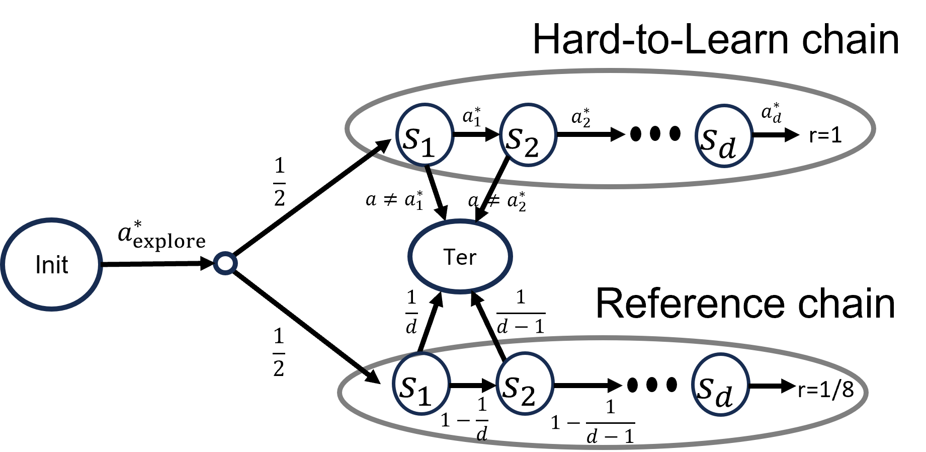
(a) Case I: $\iota=\iota_{\text{hard}}$ does not reveal anything. The probability to get $\iota=\iota_{hard}$ is larger than $1/4$.

(b) Case II: $\iota\neq\iota_{\text{hard}}$ nearly specifies the true context. In this case, one context $m(\iota)\in[M/2+1,...,M]$ has a strong prior, i.e., $\mathds{P}(m(\iota)|\iota)\geq 1/2$.

Figure 1: Hard instance. Optimal behaviors is denoted with the set of actions $\{a_{i}^{*}\}_{i=1}^{d}$. The numbers on the arrow represent the probability of transitions under the optimal policy. The symbol $a\neq\bar{a}$ next to an arrow means that all actions that are not $\bar{a}$ result with the described transition.

Next, we describe the lower bound construction and supply intuition for this result. Consider the following scenario (see Figure 1 for the class of LMDP-$\Psi$s): suppose that for a non-negligible portion of episodes, the prospective side information does supply any information on the latent context. That is, given the prospective side information $\iota_{\text{hard}}$ the posterior probability over the latent contexts is uniform, i.e., $\mathds{P}(m|\iota_{\text{hard}})=1/M$, and $\iota_{\text{hard}}$ happens with constant probability, e.g., $1/4$. With $\iota_{\text{hard}}$ alone, however, learning the optimal action sequence $a_{1:d}^{*}$ (optimal policy) may suffer from an exponential lower bound $A^{\Omega(M)}$ since $\iota_{\text{hard}}$ supplies no information on the latent context. At the same time, playing any sub-optimal action sequence incurs an $\Omega(\epsilon)$ regret where $\epsilon$ is the required target accuracy.

On the other hand, any other prospective side information $\iota\neq\iota_{\text{hard}}$, provides a strong signal of one environment that is the most likely, i.e., $\mathds{P}(m^{*}(\iota)|\iota)\geq 1/2$. Further, suppose that there is a unique exploiting action for each context that always gives a high reward, and playing any other action incurs $O(1)$-regret. For this environment, the regret of any algorithm is proportional to how many times the sub-optimal action is played when $\iota\neq\iota_{\text{hard}}$.

However, it is still essential to learn the optimal sequence of actions $a_{1:d}^{*}$ in order to behave optimally under $\iota_{\text{hard}}$. Therefore, to avoid the exponential lower bound, we should be aided by good prospective side information $\iota\neq\iota_{\text{hard}}$ despite the strong signal of the underlying model. We can construct internal dynamics such that we need to explore the two chains for at least $\Omega(A/\alpha^{2}\epsilon^{2})$ episodes to identify the optimal action sequence $a_{1:d}^{*}$ when $\iota\neq\iota_{\text{hard}}$. Combining these arguments, the regret lower bound should be at least $\min\left(\frac{A^{\Omega}(M)}{\epsilon},\frac{A}{\alpha^{2}\epsilon^{2}},K\epsilon\right)$, yielding Theorem 4.2.

To obtain the multiplicative dependence on $\alpha$ and $\epsilon$, the actual construction of the hard instance family is slightly more complicated. We assume that $M$ is sufficiently large and a multiple of 4, and let $d=M/4$. We also assume that $\alpha\ll 1$ is a sufficiently small constant. We let the time step start from $t=0$ at the initial state $s_{\text{init}}$. Next, we describe the construction of the hard LMDP-$\Psi$ class:

State Space.

There are four categories of states. The initial state $s_{\text{init}}$, absorbing state $s_{\text{ter}}$ (which means essentially an episode is terminated), a chain of states constructing a hard-to-learn system $s^{\text{hard}}_{1:d}$, and another chain of states constructing a reference system $s^{\text{ref}}_{1:d}$.

Action Space.

The set of actions at the initial time step consists of a set of candidate exploring actions $\mathcal{A}_{\text{explore}}$ and exploiting actions $\mathcal{A}_{\text{exploit}}:=\{a^{m}_{\text{exploit}}\}_{m=M/2+1}^{M}$ that control the dynamics at the initial state. The action set at time steps $1,\cdots,d$, denoted by $\mathcal{A}_{\text{control}}$, controls the dynamics in hard-to-learn and reference chains of the system. At the initial time step, only one action of $\mathcal{A}_{\text{explore}}$ is a true exploring action $a_{\text{explore}}^{*}$. At time steps $1,\cdots,d$ only one action sequence $a_{1:d}^{*}\in\mathcal{A}_{\text{control}}^{\bigotimes d}$ is the optimal sequence.

Latent Environments and Initial Dynamics.

There are three groups of MDPs: $\mathcal{G}_{\texttt{learn}}$, $\mathcal{G}_{\texttt{ref}}$, and $\mathcal{G}_{\texttt{obs}}$. All MDPs always start from the same starting state $s_{\text{init}}$.

$\mathcal{G}_{\texttt{learn}}$ consists of $(M/4)$ MDPs, $\mathcal{M}_{1},...,\mathcal{M}_{M/4}$, which essentially form the hard to learn example from Kwon et al. (2021) when no prospective side information is provided. In any of these environments, in the beginning, when the ‘true’ explore action $a_{\text{explore}}^{*}$ is played, it transitions to the starting of hard-instance chain $s^{\text{hard}}_{1}$ with some small probability.

Similarly, $\mathcal{G}_{\texttt{ref}}$ consists of another $(M/4)$ MDPs, $\mathcal{M}_{M/4+1},...,\mathcal{M}_{M/2}$, and the purpose of $\mathcal{G}_{\texttt{ref}}$ is to confuse the learning the optimal action sequence in the hard-to-learn chain, as we make the prospective side information hard to distinguish whether an MDP belongs to $\mathcal{G}_{\texttt{learn}}$ or $\mathcal{G}_{\texttt{ref}}$. More precisely, under $\iota_{\text{hard}}$, it is hard to identify which one is the hard-to-learn or reference chain, and thus it is hard to identify $a_{\text{explore}}^{*}$. This is crucial to build a multiplicative lower bound on $\alpha$ and $\epsilon$.

The rest of $(M/2)$ MDPs, indexed by $\mathcal{M}_{M/2+1},...,\mathcal{M}_{M}$, belong to the almost observable group $\mathcal{G}_{\texttt{obs}}$. In each environment of this group $\mathcal{M}_{m}\in\mathcal{G}_{\texttt{obs}}$ where $m=M/2+1,...,M$, executing $a^{m}_{\text{exploit}}$ at the initial time step step results with a reward 1, and gets 0 otherwise.

Dynamics of Two Chains.

In both hard and reference chains, at any states in $s_{1:d}^{\text{hard}}$ and $s_{1:d}^{\text{ref}}$, all actions $a\notin\mathcal{A}_{\text{control}}$ invoke transitions to $s_{\text{ter}}$ with 0 rewards.

In the reference chain, in all environments in $\mathcal{G}_{\texttt{learn}}\cup\mathcal{G}_{\texttt{ref}}$, for all actions $a\in\mathcal{A}_{\text{control}}$, $s_{t}^{\text{ref}}$ transitions to $s_{t+1}^{\text{ref}}$ with probability $\left(1-\frac{1}{d+1-t}\right)$ and transitions to $s^{\text{ter}}$ otherwise when $t<d$. When the chain transitions to $s_{\text{ter}}$, we receive a reward sampled from $\mathrm{Ber}(1/8)$.

In the hard-to-learn chain, for all environments in $\mathcal{G}_{\texttt{ref}}$, the system dynamic is identical to the reference chain. The environments in $\mathcal{G}_{\texttt{learn}}$ are set to be the hard family instances of MDPs from Kwon et al. (2021) (while setting $d=M/4$), also depicted in Figure 1, Case I:

1. At each time, MDPs in $\mathcal{G}_{\texttt{learn}}$ transitions from one state in the chain to the next state or to $s_{\text{ter}}$ depending on the played action. When an agent transitions to $s_{\text{ter}}$ it receives a reward drawn from $\mathrm{Ber}(1/8)$.

2. At all time steps besides at the last one, the agent receives a reward of $0$, when taking an action that does not take it to $s_{\text{ter}}$. At the last time step, if the agent did not move to $s_{\text{ter}}$ and upon taking the action $a_{d}^{*}$ it recives a reward of $1$. Hence, the essence of this construction is to identify the optimal action sequence $a_{1:d}^{*}$ which guarantees a reward $1$ from $\mathcal{M}_{1}$ at the end of the chain $s_{d}^{\text{hard}}$. Playing any sub-optimal action sequence generates the distribution of observations indistinguishable from the reference chain.

We complete the construction in Appendix C.

Prospective Side Information.

The prospective side information either is a strong prior of one of the MDPs in $\mathcal{G}_{\texttt{obs}}$, or uninformative in which case $\iota=\iota_{\text{hard}}$. Our construction ensures that when observing $\iota_{\text{hard}}$, all MDPs in $\mathcal{G}_{\text{learn}}$ and $\mathcal{G}_{\text{ref}}$ have equal conditional probability, i.e., $\mathds{P}(m|\iota)=2/M$ for all $m\in[M/2]$, whereas for other values of prospective information $\iota\neq\iota_{\text{hard}}$, there is one MDP from $\mathcal{G}_{\text{obs}}$ whose prior probability is greater than $1/2$, and priors over $\mathcal{G}_{\text{learn}}\cup\mathcal{G}_{\text{ref}}$ are nearly equally distributed but perturbed by a small parameter $\alpha$, i.e., $\mathds{P}(m_{\text{obs}}|\iota)\geq 1/2$ for some $m_{\text{obs}}\in[M/2+1,M]$, and $\mathds{P}(m|\iota)=O(1/M)+O(\alpha)$ for all $m\in[M/2]$.

Hard Instances.

The family of hard instances $\Theta_{\text{hard}}$ that consists the set of hard-to-learn LMDP-$\Psi$s is described as follows. All instances in the hard instance family shares the same state space, action space and prospective side-information. The family of hard-to-learn LMDP-$\Psi$s differ in their transition dynamics. Each LMDP-$\Psi$ in $\Theta_{\text{hard}}$ differs by its transition dynamics. The transition dynamics of each element of $\Theta_{\text{hard}}$ is determined by one of the possible sequence $a^{*}_{1:d}\in\mathcal{A}_{\text{control}}^{\bigotimes d}$ that represents the optimal action sequence, and by the ‘true’ exploring actions $a_{\text{explore}}^{*}\in\mathcal{A}_{\text{explore}}$.

Reference Model.

We denote $\theta_{0}$ as the reference model whose hard-to-learn chain is no different from the reference chain in all individual MDPs. In the reference model, at $s_{\text{init}}$, all MDPs in $\mathcal{G}_{\texttt{ref}}$ transitions to $s_{1}^{\text{hard}}$ and those in $\mathcal{G}_{\texttt{learn}}$ transitions to $s_{1}^{\text{ref}}$ deterministically when any action in $\mathcal{A}_{\text{explore}}$ is played. All other parts are constructed with the same dynamics as in $\Theta_{\text{hard}}$.

Proof Overview.

With the above construction, the following lemmas play key roles in proving the regret lower bound:

Lemma 5.2

Let $\psi$ be any exploration strategy for LMDP-$\Psi$. Consider any hard instance $\theta\in\Theta_{\text{hard}}$ and the reference model $\theta_{0}$. Let $N_{\psi,\iota,a_{1:d}}^{\text{explore}}(K)$ be the number of times that explored the chain systems with the test $t_{\iota}(a_{1:d}):=\{\iota,a_{\text{explore}}^{*},a_{1:d}\}$, i.e., with the true exploration action and any sequence $a_{1:d}\in\mathcal{A}^{\bigotimes d}$ given prospective side information $\iota$. Then,

$$\sum_{\iota,a_{1:d}}\mathbb{E}_{\theta_{0}} \left[N_{\psi,\iota,a_{1:d}}^{\text{explore}}(K)\right]\cdot\textrm{KL}\left(\mathds{P}_{\theta_{0}}(\cdot|t_{\iota}(a_{1:d}),\mathds{P}_{\theta}(\cdot|t_{\iota}(a_{1:d})\right)=\textrm{KL}\left(\mathds{P}^{\psi}_{\theta_{0}}(\tau^{1:K}),\mathds{P}^{\psi}_{\theta}(\tau^{1:K})\right),$$ (8)

where $\mathds{P}^{\psi}(\tau^{1:K})$ is a distribution of $K$ trajectories obtained with the exploration strategy $\psi$.

The main reason for the equality (8) is that whenever $a\neq a^{*}_{\text{explore}}$ is played regardless of the prospective side information, the two models $\theta$ and $\theta_{0}$ generate observations from the same distribution. Then the key lemma is on the bounds for the conditional KL-divergence:

Lemma 5.3

For all non optimal action sequences $a_{1:d}\neq a_{1:d}^{*}$, the following holds:

$$\textrm{KL}\left(\mathds{P}_{\theta_{0}}(\cdot|\iota_{\text{hard}},a_{\text{explore}}^{*},a_{1:d}),\mathds{P}_{\theta}(\cdot|\iota_{\text{hard}},a_{\text{explore}}^{*},a_{1:d})\right)=0,$$

and for all $\iota\in\mathcal{I}$,

$$\textrm{KL}\left(\mathds{P}_{\theta_{0}}(\cdot|\iota,a_{\text{explore}}^{*},a_{1:d}^{*}),\mathds{P}_{\theta}(\cdot|\iota,a_{\text{explore}}^{*},a_{1:d}^{*})\right)\lesssim\epsilon^{2}.$$

Furthermore, for all $\iota\neq\iota_{\text{hard}}$ and $a_{1:d}\neq a_{1:d}^{*}$:

$$\textrm{KL}\left(\mathds{P}_{\theta_{0}}(\cdot|\iota,a_{\text{explore}}^{*},a_{1:d}),\mathds{P}_{\theta}(\cdot|\iota,a_{\text{explore}}^{*},a_{1:d})\right)\lesssim(\alpha\epsilon)^{2}.$$

Therefore, we can bound the KL-divergence between the total trajectory distributions of the two models as

$$\textrm{KL}\left(\mathds{P}^{\psi}_{\theta_{0}}(\tau^{1:K}),\mathds{P}^{\psi}_{\theta}(\tau^{1:K})\right)\leq\mathbb{E}_{\theta_{0}}[N_{\psi,\iota_{\text{hard}},a_{1:d}^{*}}^{\text{explore}}]\epsilon^{2}+\sum_{\iota\neq\iota_{\text{hard}},a_{1:d}}\mathbb{E}_{\theta_{0}}[N_{\psi,\iota,a_{1:d}}^{\text{explore}}](\alpha\epsilon)^{2},$$

which translates to the impossibility of distinguishing the two with a probability more than $2/3$ unless either

$$\mathbb{E}_{\theta_{0}}[N_{\psi,\iota_{\text{hard}},a_{1:d}^{*}}^{\text{explore}}(K)]\gtrsim\frac{1}{\epsilon^{2}},\text{or }\sum_{\iota\neq\iota_{\text{hard}},a_{1:d}}\mathbb{E}_{\theta_{0}}[N_{\psi,\iota,a_{1:d}}^{\text{explore}}(K)]\gtrsim\frac{1}{\alpha^{2}\epsilon^{2}}.$$ (9)

Finally, note that playing sub-optimal actions with $\iota\neq\iota_{\text{hard}}$ incurs at least $1/8$-regret, playing sub-optimal action sequence $a_{1:d}\neq a_{1:d}^{*}$ incurs at least $O(\epsilon/M)$-regret, and playing the optimal sequence $a_{1:d}^{*}$ at least $O(1/\epsilon^{2})$ times would take $(A^{d}/\epsilon^{2})$ episodes in the worst case. The remaining steps are to formally state the ideas (see Appendix C).

6 Conclusion

In this work, we introduced the LMDP-$\Psi$ setting, when a prospective and weakly revealing information on the latent context is given to an agent. We showed that LMDP-$\Psi$ does not belong to the weakly revealing POMDP class, due to the correlation between observations at different time steps. Further, our results highlight its fundamental different characteristic: we derived an $\Omega(K^{2/3})$ lower bound on its regret, and, hence, the standard $O(\sqrt{K})$ worst-case upper bound is not achievable in general for this class of problems. We also derived a matching $O(K^{2/3})$ upper bound to complete our results.

From a broader perspective, our results highlight a key deficiency of a ubiquitous assumption made in POMDP modeling, namely, the independence of observation between consecutive time steps, when conditioning on the latent state. We believe that studying the learnability of more general POMDP settings with prospective side information, or non-trivial correlation between observations serves as a fruitful ground for future work. Further, scaling the methods for practical settings, while building on solid theoretical grounds, is a valuable and open research direction.

Appendix A Auxiliary Lemmas

Lemma A.1 (General MLE, Liu et al. [2022])

With probability $1-\delta$ for any $\delta>0$, for all $k\in[K]$, $t\in[H]$ and for any $\theta\in\Theta$,

$$\sum_{(\iota,\tau_{t},\pi)\in\mathcal{D}^{k}}\log(\mathds{P}^{\pi}_{\theta}(\iota,\tau_{t}))-3\log(K|\Theta|/\delta)\leq\sum_{(\iota,\tau_{t},\pi)\in\mathcal{D}^{k}}\log(\mathds{P}^{\pi}_{\theta^{*}}(\iota,\tau_{t})).$$ (10)

This is by now a standard MLE technique for constructing confidence sets in RL Agarwal et al. [2020].

Proof.

The proof follows a Chernoff bound type of technique:

$$\mathds{P}_{\theta^{*}} \left(\sum_{(\iota,\tau_{t},\pi)\in\mathcal{D}^{k}}\log\left(\frac{\mathds{P}^{\pi}_{\theta}(\iota,\tau_{t})}{\mathds{P}^{\pi}_{\theta^{*}}(\iota,\tau_{t})}\right)\geq\mathbb{E}_{\theta^{*}}\left[\sum_{(\iota,\tau_{t},\pi)\in\mathcal{D}^{k}}\log\left(\frac{\mathds{P}^{\pi}_{\theta}(\iota,\tau_{t})}{\mathds{P}^{\pi}_{\theta^{*}}(\iota,\tau_{t})}\right)\right]+\beta\right)$$

$$\leq\mathds{P}_{\theta^{*}}\left(\exp\left(\sum_{(\iota,\tau_{t},\pi)\in\mathcal{D}^{k}}\log\left(\frac{\mathds{P}^{\pi}_{\theta}(\iota,\tau_{t})}{\mathds{P}^{\pi}_{\theta^{*}}(\iota,\tau_{t})}\right)\right)\geq\exp\left(\beta\right)\right)$$

$$\leq\mathbb{E}_{\theta^{*}}\left[\exp\left(\sum_{(\iota,\tau_{t},\pi)\in\mathcal{D}^{k}}\log\left(\frac{\mathds{P}^{\pi}_{\theta}(\iota,\tau_{t})}{\mathds{P}^{\pi}_{\theta^{*}}(\iota,\tau_{t})}\right)\right)\right]\exp(-\beta).$$

Note that random variables are $(\iota,\tau_{t},\pi)$ in the trajectory dataset $\mathcal{D}^{k}$, and

$$\mathbb{E}_{\theta^{*}}\left[\sum_{(\tau,\pi)\in\mathcal{D}^{k}}\log\left(\frac{\mathds{P}^{\pi}_{\theta}(\iota,\tau_{t})}{\mathds{P}^{\pi}_{\theta^{*}}(\iota,\tau_{t})}\right)\right]=-\textrm{KL}(\mathds{P}_{\theta^{*}}(\mathcal{D}^{k})||\mathds{P}_{\theta}(\mathcal{D}^{k}))\leq 0,$$

and further notice the last inequality is by Markov’s inequality. Then,

$$\mathbb{E}_{\theta^{*}}\left[\exp\left(\sum_{(\iota,\tau_{t},\pi)\in\mathcal{D}^{k}}\log\left(\frac{\mathds{P}^{\pi}_{\theta}(\iota,\tau_{t})}{\mathds{P}^{\pi}_{\theta^{*}}(\iota,\tau_{t})}\right)\right)\right] =\mathbb{E}_{\theta^{*}}\left[\Pi_{(\iota,\tau_{t},\pi)\in\mathcal{D}^{k}}\frac{\mathds{P}^{\pi}_{\theta}(\iota,\tau_{t})}{\mathds{P}^{\pi}_{\theta^{*}}(\iota,\tau_{t})}\right]=\sum_{\iota,\tau_{t}}\mathds{P}^{\pi}_{\theta}(\iota,\tau_{t})=1.$$

Combining the above, taking a union bound over $k\in[K]$ and $\theta\in\Theta$, letting $\beta=\log(K|\Theta|/\delta)$, with probability $1-\delta$, the inequality in equality (10) holds. ∎

Lemma A.2

With probability $1-\delta$, for all $k\in[K]$, $t\in[H]$ and $\theta\in\Theta$, we have

$$\sum_{\left(\iota,\tau,\pi\right)\in\mathcal{D}^{k}}d_{\texttt{TV}}^{2}\left(\mathds{P}_{\theta}^{\pi}(\iota,\tau),\mathds{P}_{\theta^{*}}^{\pi}(\iota,\tau)\right)\lesssim\sum_{(\iota,\tau,\pi)\in\mathcal{D}^{k}}\log\left(\frac{\mathds{P}_{\theta^{*}}^{\pi}(\iota,\tau)}{\mathds{P}_{\theta}^{\pi}(\iota,\tau)}\right)+\beta,$$

$$\sum_{\left(\iota,\tau,\pi\right)\in\mathcal{D}^{k}}d_{\texttt{H}}^{2}\left(\mathds{P}_{\theta}^{\pi}(\iota,\tau),\mathds{P}_{\theta^{*}}^{\pi}(\iota,\tau)\right)\lesssim\sum_{(\iota,\tau,\pi)\in\mathcal{D}^{k}}\log\left(\frac{\mathds{P}_{\theta^{*}}^{\pi}(\iota,\tau)}{\mathds{P}_{\theta}^{\pi}(\iota,\tau)}\right)+\beta.$$

Proof.

By the TV-distance and Hellinger distance relation, for any $\iota,\tau$, $\pi$ and $t\in[H]$,

$$d_{\texttt{TV}}^{2}\left(\mathds{P}_{\theta}^{\pi}(\iota,\tau),\mathds{P}_{\theta^{*}}^{\pi}(\iota,\tau)\right) \leq 2d_{\texttt{H}}^{2}\left(\mathds{P}_{\theta}^{\pi}(\iota,\tau),\mathds{P}_{\theta^{*}}^{\pi}(\iota,\tau)\right)$$

$$=2\left(1-\mathbb{E}_{\iota,\tau\sim\mathds{P}_{\theta^{*}}^{\pi}}\left[\sqrt{\frac{\mathds{P}_{\theta}^{\pi}(\iota,\tau)}{\mathds{P}_{\theta^{*}}^{\pi}(\iota,\tau)}}\right]\right)$$

$$\leq-2\log\left(\mathbb{E}_{\iota,\tau\sim\mathds{P}_{\theta^{*}}^{\pi}}\left[\sqrt{\frac{\mathds{P}_{\theta}^{\pi}(\iota,\tau)}{\mathds{P}_{\theta^{*}}^{\pi}(\iota,\tau)}}\right]\right).$$

To bound the summation over samples, we start from

$$\sum_{\left(\iota,\tau,\pi\right)\in\mathcal{D}^{k}}d_{\texttt{TV}}^{2}\left(\mathds{P}_{\theta}^{\pi}(\iota,\tau),\mathds{P}_{\theta^{*}}^{\pi}(\iota,\tau)\right) \leq-2\sum_{\left(\iota,\tau,\pi\right)\in\mathcal{D}^{k}}\log\left(\mathbb{E}_{\iota,\tau\sim\mathds{P}_{\theta^{*}}^{\pi}}\left[\sqrt{\frac{\mathds{P}_{\theta}^{\pi}(\iota,\tau)}{\mathds{P}_{\theta^{*}}^{\pi}(\iota,\tau)}}\right]\right).$$

On the other hand, by the Chernoff bound,

$$\mathds{P}_{\theta^{*}} \left(\sum_{(\iota,\tau,\pi)\in\mathcal{D}^{k}}\log\left(\sqrt{\frac{\mathds{P}_{\theta}^{\pi}(\iota,\tau)}{\mathds{P}_{\theta^{*}}^{\pi}(\iota,\tau)}}\right)\geq\sum_{(\iota,\tau,\pi)\in\mathcal{D}^{k}}\log\mathbb{E}_{\iota,\tau\sim\mathds{P}_{\theta^{*}}^{\pi}}\left[\sqrt{\frac{\mathds{P}_{\theta}^{\pi}(\iota,\tau)}{\mathds{P}_{\theta^{*}}^{\pi}(\iota,\tau)}}\right]+\beta\right)$$

$$\leq\mathbb{E}_{\theta^{*}}\left[\frac{\exp\left(\sum_{(\iota,\tau,\pi)\in\mathcal{D}^{k}}\log\left(\sqrt{\frac{\mathds{P}^{\pi}_{\theta}(\iota,\tau)}{\mathds{P}^{\pi}_{\theta^{*}}(\iota,\tau)}}\right)\right)}{\exp\left(\sum_{(\iota,\tau,\pi)\in\mathcal{D}^{k}}\log\mathbb{E}_{\iota,\tau\sim\mathds{P}_{\theta^{*}}^{\pi}}\left[\sqrt{\frac{\mathds{P}_{\theta}^{\pi}(\iota,\tau)}{\mathds{P}_{\theta^{*}}^{\pi}(\iota,\tau)}}\right]\right)}\right]\exp(-\beta)$$

$$=\mathbb{E}_{\theta^{*}}\left[\frac{\Pi_{(\iota,\tau,\pi)\in\mathcal{D}^{k}}\sqrt{\frac{\mathds{P}_{\theta}^{\pi}(\iota,\tau)}{\mathds{P}_{\theta^{*}}^{\pi}(\iota,\tau)}}}{\Pi_{(\iota,\tau,\pi)\in\mathcal{D}^{k}}\mathbb{E}_{\iota,\tau\sim\mathds{P}_{\theta^{*}}^{\pi}}\left[\sqrt{\frac{\mathds{P}_{\theta}^{\pi}(\iota,\tau)}{\mathds{P}_{\theta^{*}}^{\pi}(\iota,\tau)}}\right]}\right]\exp(-\beta)$$

$$=\mathbb{E}_{\theta^{*}}\left[\frac{\Pi_{(\iota,\tau,\pi)\in\mathcal{D}^{k-1}}\sqrt{\frac{\mathds{P}_{\theta}^{\pi}(\iota,\tau)}{\mathds{P}_{\theta^{*}}^{\pi}(\iota,\tau)}}\cdot\mathbb{E}_{\iota,\tau^{k}\sim\mathds{P}_{\theta^{*}}^{\pi^{k}}}\left[\sqrt{\frac{\mathds{P}^{\pi^{k}}_{\theta}(\iota,\tau^{k})}{\mathds{P}^{\pi}_{\theta^{*}}(\iota,\tau^{k})}}\Big{|}\pi^{k},\mathcal{\mathcal{D}}^{k-1}\right]}{\Pi_{(\iota,\tau,\pi)\in\mathcal{D}^{k}}\mathbb{E}_{\iota,\tau\sim\mathds{P}_{\theta^{*}}^{\pi}}\left[\sqrt{\frac{\mathds{P}^{\pi}_{\theta}(\iota,\tau)}{\mathds{P}^{\pi}_{\theta^{*}}(\iota,\tau)}}\right]}\right]\exp(-\beta)$$

$$=\mathbb{E}_{\theta^{*}}\left[\frac{\Pi_{(\iota,\tau,\pi)\in\mathcal{D}^{k-1}}\sqrt{\frac{\mathds{P}^{\pi}_{\theta}(\iota,\tau)}{\mathds{P}^{\pi}_{\theta^{*}}(\iota,\tau)}}}{\Pi_{(\iota,\tau,\pi)\in\mathcal{D}^{k-1}}\mathbb{E}_{\iota,\tau\sim\mathds{P}_{\theta^{*}}^{\pi}}\left[\sqrt{\frac{\mathds{P}^{\pi}_{\theta}(\iota,\tau)}{\mathds{P}^{\pi}_{\theta^{*}}(\iota,\tau)}}\right]}\right]\exp(-\beta)=...=\exp(-\beta),$$

where in the last line, we used the tower property of expectation. Thus, again by setting $\beta=O\left(\log(KH|\Theta|/\delta)\right)$, with probability at least $1-\delta$, we have

$$\sum_{(\iota,\tau,\pi)\in\mathcal{D}^{k}} d_{\texttt{TV}}^{2}(\mathds{P}_{\theta}^{\pi}(\iota,\tau),\mathds{P}_{\theta^{*}}^{\pi}(\iota,\tau))\lesssim-\frac{1}{2}\sum_{(\iota,\tau,\pi)\in\mathcal{D}^{k}}\log\left(\frac{\mathds{P}^{\pi}_{\theta}(\iota,\tau)}{\mathds{P}^{\pi}_{\theta^{*}}(\iota,\tau)}\right)+\beta$$

$$=-\frac{1}{2}\sum_{(\iota,\tau,\pi)\in\mathcal{D}^{k}}\log\left(\frac{\mathds{P}^{\pi}_{\theta}(\iota,\tau)}{\mathds{P}^{\pi}_{\theta^{*}}(\iota,\tau)}\right)+\frac{1}{2}\sum_{(\iota,\tau,\pi)\in\mathcal{D}^{k}}\log\left(\frac{\mathds{P}^{\pi}_{\theta}(\iota,\tau)}{\mathds{P}^{\pi}_{\theta^{*}}(\iota,\tau)}\right)+\beta.$$

We can apply Lemma A.1, and finally have

$$\sum_{(\iota,\tau,\pi)\in\mathcal{D}^{k}} d_{\texttt{TV}}^{2}(\mathds{P}_{\theta}^{\pi}(\iota,\tau),\mathds{P}_{\theta^{*}}^{\pi}(\iota,\tau))\lesssim-\sum_{(\iota,\tau,\pi)\in\mathcal{D}^{k}}\log\left(\frac{\mathds{P}^{\pi}_{\theta}(\iota,\tau)}{\mathds{P}^{\pi}_{\theta^{*}}(\iota,\tau)}\right)+\beta.$$

∎

Most of the following lemmas can also be found in Huang et al. [2023] as we adopt their proof strategy. We state and prove them for the completeness. The following is the concentration lemma for the empirical conditional probability, which Importantly, this property still holds regardless of causal relationships inside each trajectory sample:

Lemma A.3

With probability $1-\delta$, for all $k\in[K]$, $t\in[H]$, $\theta\in\Theta$, we have

$$\sum_{\left(\iota,\tau_{t},\omega_{t},\pi\right)\in\mathcal{D}^{k}}d_{\texttt{TV}}^{2}\left(\mathds{P}_{\theta}^{\pi}(\iota,\omega_{t}|\tau_{t}),\mathds{P}_{\theta^{*}}^{\pi}(\iota,\omega_{t}|\tau_{t})\right)\lesssim\sum_{(\iota,\tau,\pi)\in\mathcal{D}^{k}}\log\left(\frac{\mathds{P}_{\theta^{*}}^{\pi}(\iota,\tau)}{\mathds{P}_{\theta}^{\pi}(\iota,\tau)}\right)+\beta,$$

$$\sum_{\left(\iota,\tau_{t},\omega_{t},\pi\right)\in\mathcal{D}^{k}}d_{\texttt{H}}^{2}\left(\mathds{P}_{\theta}^{\pi}(\iota,\omega_{t}|\tau_{t}),\mathds{P}_{\theta^{*}}^{\pi}(\iota,\omega_{t}|\tau_{t})\right)\lesssim\sum_{(\iota,\tau,\pi)\in\mathcal{D}^{k}}\log\left(\frac{\mathds{P}_{\theta^{*}}^{\pi}(\iota,\tau)}{\mathds{P}_{\theta}^{\pi}(\iota,\tau)}\right)+\beta.$$

Proof.

The proof is almost identical except that we now start from

$$\sum_{\left(\tau,\pi\right)\in\mathcal{D}^{k}}d_{\texttt{TV}}^{2}\left(\mathds{P}_{\theta}^{\pi}(\iota,\omega_{t}|\tau_{t}),\mathds{P}_{\theta^{*}}^{\pi}(\iota,\omega_{t}|\tau_{t})\right) \leq-2\sum_{\left(\tau,\pi\right)\in\mathcal{D}^{k}}\log\left(\mathbb{E}_{(\iota,\omega_{t})\sim\mathds{P}_{\theta^{*}}^{\pi}(\cdot|\tau_{t})}\left[\sqrt{\frac{\mathds{P}_{\theta}^{\pi}(\iota,\omega_{t}|\tau_{t})}{\mathds{P}_{\theta^{*}}^{\pi}(\iota,\omega_{t}|\tau_{t})}}\right]\right).$$

and use the tower property of expectation conditioned on $\tau_{t}^{k}$. Thus, again by setting $\beta=O\left(\log(KH|\Theta|/\delta)\right)$, with probability at least $1-\delta$, we have

$$\sum_{\left(\tau,\pi\right)\in\mathcal{D}^{k}}d_{\texttt{TV}}^{2}\left(\mathds{P}_{\theta}^{\pi}(\iota,\omega_{t}|\tau_{t}),\mathds{P}_{\theta^{*}}^{\pi}(\iota,\omega_{t}|\tau_{t})\right)\lesssim-\frac{1}{2}\sum_{(\tau,\pi)\in\mathcal{D}^{k}}\log\left(\frac{\mathds{P}^{\pi}_{\theta}(\iota,\omega_{t}|\tau_{t})}{\mathds{P}^{\pi}_{\theta^{*}}(\iota,\omega_{t}|\tau_{t})}\right)+\beta$$

$$=-\frac{1}{2}\sum_{(\iota,\tau,\pi)\in\mathcal{D}^{k}}\log\left(\frac{\mathds{P}^{\pi}_{\theta}(\iota,\tau)}{\mathds{P}^{\pi}_{\theta^{*}}(\iota,\tau)}\right)+\frac{1}{2}\sum_{(\iota,\tau,\pi)\in\mathcal{D}^{k}}\log\left(\frac{\mathds{P}^{\pi}_{\theta}(\tau_{t})}{\mathds{P}^{\pi}_{\theta^{*}}(\tau_{t})}\right)+\beta.$$

Finally, we apply Lemma A.1, and have

$$\sum_{\left(\iota,\tau,\pi\right)\in\mathcal{D}^{k}}d_{\texttt{TV}}^{2}\left(\mathds{P}_{\theta}^{\pi}(\iota,\omega_{t}|\tau_{t}),\mathds{P}_{\theta^{*}}^{\pi}(\iota,\omega_{t}|\tau_{t})\right)\lesssim-\sum_{(\iota,\tau,\pi)\in\mathcal{D}^{k}}\log\left(\frac{\mathds{P}^{\pi}_{\theta}(\iota,\tau)}{\mathds{P}^{\pi}_{\theta^{*}}(\iota,\tau)}\right)+\beta.$$

∎

Lemma A.4

For arbitrary probability distribution $P,Q$ over joint distributions $(\tau,\omega)$,

$$\mathbb{E}_{\tau\sim P}[d_{\texttt{H}}^{2}(P(\omega|\tau),Q(\omega|\tau))]\leq 4d_{\texttt{H}}^{2}(P(\omega,\tau),Q(\omega,\tau)).$$

Proof.

We prove this statement by explicitly bounding the Hellinger distance.

$$\int\left(\int\left(\sqrt{P(\omega|\tau)}-\sqrt{Q(\omega|\tau)}\right)^{2}d\omega\right)P(\tau)d\tau$$

$$\leq 2\int\int\left(\sqrt{P(\omega,\tau)}-\sqrt{Q(\tau)Q(\omega|\tau)}\right)^{2}d\omega d\tau+2\int\int\left(\sqrt{P(\tau)Q(\omega|\tau)}-\sqrt{Q(\tau)Q(\omega|\tau)}\right)^{2}d\omega d\tau$$

$$=2d_{\texttt{H}}^{2}(P(\omega,\tau),Q(\omega,\tau))+2\int\int\left(\sqrt{P(\tau)}-\sqrt{Q(\tau)}\right)^{2}Q(\omega|\tau)d\omega d\tau$$

$$\leq 4d_{\texttt{H}}^{2}(P(\omega,\tau),Q(\omega,\tau)).$$

∎

Lemma A.5

Let $x\in\mathbb{R}^{d}$ be a random vector from a series of distributions $\{\mathcal{D}^{k}\}_{k}$ and let $U_{k}=U_{1}+\sum_{j<k}\mathbb{E}_{x\sim\mathcal{D}^{j}}[xx^{\top}]$ with $U_{1}\succeq\lambda I$ for some positive constant $\lambda>0$. Assume that $\|x\|_{2}\leq 1$ almost surely. Then,

$$\sum_{k=1}^{K}\min\left(\mathbb{E}_{x\sim\mathcal{D}^{k}}\left[\|x\|^{2}_{U_{k}^{-1}}\right],R\right)\leq(1+R)d\log(1+K/\lambda).$$

This is minor variation of the standard result from Abbasi-Yadkori et al. [2011]. Differently from their result, here, we need to establish the bound for the expected $U_{k}$. Hence their result is not directly applied here.

Proof.

We follow the same technique of Abbasi-Yadkori et al. [2011].

$$\sum_{k=1}^{K}\min\left(\mathbb{E}_{x\sim\mathcal{D}^{k}}\left[\|x\|^{2}_{U_{k}^{-1}}\right],R\right) \leq(1+R)\sum_{k=1}^{K}\log\left(1+\mathbb{E}_{x\sim\mathcal{D}^{k}}\left[\|x\|^{2}_{U_{k}^{-1}}\right]\right)$$

$$\stackrel{{\scriptstyle(a)}}{{=}}(1+R)\sum_{k=1}^{K}\log\left(1+\texttt{Tr}(\mathbb{E}_{x\sim\mathcal{D}^{k}}\left[xx^{\top}\right]U_{k}^{-1})\right)$$

$$=(1+R)\sum_{k=1}^{K}\log\left(1+\texttt{Tr}((U_{k+1}-U_{k})U_{k}^{-1})\right)$$

$$\leq(1+R)\sum_{k=1}^{K}\log\texttt{det}\left(I_{d}+(U_{k}^{-1/2}(U_{k+1}-U_{k})U_{k}^{-1/2})\right)$$

$$=(1+R)\sum_{k=1}^{K}\log\frac{\texttt{det}U_{k+1}}{\texttt{det}(U_{k})}=(1+R)\log\frac{\texttt{det}(U_{K+1})}{\texttt{det}(U_{1})}$$

$$\leq(1+R)d\log(1+K/\lambda),$$

where $(a)$ is due to the linearity of trace operators. ∎

Lemma A.6

Let $x_{k}$ be any sequence of vectors in $\mathbb{R}^{d}$ where $\textbf{rank}(\{x_{k}\}_{k})=r<d$, and let $U_{k}=\lambda I+\sum_{j<k}x_{j}x_{j}^{\top}$. Then,

$$\sum_{j<k}\|x_{k}\|_{U_{k}^{-1}}^{2}\leq r.$$

Proof.

Again, we can express $a^{\top}A^{-1}a=\texttt{Tr}(aa^{\top}A^{-1})$, and thus

$$\sum_{j<k}\texttt{Tr}(x_{j}x_{j}^{\top}U_{k}^{-1}) =\texttt{Tr}\left((\textstyle\sum_{j<k}x_{j}x_{j}^{\top})U_{k}^{-1}\right)$$

$$=\texttt{Tr}\left(I-\left(I+\lambda^{-1}\textstyle\sum_{j<k}x_{j}x_{j}^{\top}\right)^{-1}\right)\leq r,$$

where the inequality holds since the matrix inside Tr is at most rank $r$ with eigenvalues less than or equal to one. ∎

Lemma A.7

For any vectors $a,b$ and positive definite matrices $A,B$ such that $A,B\succeq\lambda_{0}I$, we have

$$\|a\|_{A^{-1}}-\|b\|_{B^{-1}}\leq\frac{1}{\sqrt{\lambda_{0}}}\|a-b\|_{2}+\|b\|_{B^{-1}}\|A^{-1/2}(B-A)B^{-1/2}\|_{2}.$$

Proof.

The proof follows by algebraic manipulations:

$$\|a\|_{A^{-1}}-\|b\|_{B^{-1}} =\frac{\|a\|_{A^{-1}}^{2}-\|b\|_{B^{-1}}^{2}}{\|a\|_{A^{-1}}+\|b\|_{B^{-1}}}$$

$$=\frac{a^{\top}A^{-1}(a-b)+(a-b)^{\top}B^{-1}b+a^{\top}A^{-1}(B-A)B^{-1}b}{\|a\|_{A^{-1}}+\|b\|_{B^{-1}}}$$

$$\leq\frac{\|a\|_{A^{-1}}\|a-b\|_{A^{-1}}+\|a-b\|_{B^{-1}}\|b\|_{B^{-1}}+a^{\top}A^{-1}(B-A)B^{-1}b}{\|a\|_{A^{-1}}+\|b\|_{B^{-1}}}$$

$$\leq\frac{1}{\sqrt{\lambda_{0}}}\|a-b\|_{2}+\|b\|_{B^{-1}}\|A^{-1/2}(B-A)B^{-1/2}\|_{2}.$$

∎

Appendix B Proof of Upper Bounds

We remind the reader some notations we frequently use in the appendix.

$$B(o,s_{+1}|s,a)=\mathbb{I}\cdot\textbf{diag}([\mathds{P}(o,s_{+1}|m,s,a)]_{m=1}^{M})\cdot\mathbb{I}^{\dagger},$$

$$b_{0}=\mathbb{I}w,$$

$$\tau_{t}=(s_{1},a_{1},o_{1},...,s_{t},a_{t}),$$

$$\omega_{t}=(o_{t},s_{t+1},a_{t+1},...,o_{H}),$$

$$\psi(\omega_{t},\iota|s_{t})^{\top}=\bm{e}_{\iota}^{\top}\cdot\Pi_{h=t}^{H}B{(o_{h},s_{h+1}|s_{h},a_{h})},$$

$$b(\tau_{t})=\Pi_{h=1}^{t-1}B{(o_{h},s_{h+1}|s_{h},a_{h})}b_{0},$$

$$\pi(\tau_{t})=\Pi_{h=1}^{t}\pi(a_{h}|s_{1},...,s_{h}),$$

$$\pi(\omega_{t}|\tau_{t})=\Pi_{h=t+1}^{H}\pi(a_{h}|s_{1},...,s_{h}).$$

We frequently use a shorthand for a pair of observations, $x_{t}:=(s_{t},a_{t})$ and $y_{t}:=(o_{t},s_{t+1})$.

B.1 Proof of Theorem 4.1

There are several analysis techniques available in previous work (e.g., Liu et al. [2022], Uehara et al. [2022], Liu et al. [2023], Chen et al. [2022], Huang et al. [2023]). Among all the above great works, we find the recent analysis of Huang et al. [2023] as particularly well-suited for our setting, and thus we adopt their proof ideas.

By the choice of model selection in the confidence set, it is sufficient to bound the sum TV-distances since

$$\sum_{k=1}^{K}V_{\theta^{*}}^{\pi_{\texttt{blind}}^{*}}-V_{\theta^{*}}^{\pi^{k}} \leq\sum_{k=1}^{K}V_{\theta^{k}}^{\pi_{k}}-V_{\theta^{*}}^{\pi^{k}}\leq H\cdot\sum_{k=1}^{K}d_{\texttt{TV}}(\mathds{P}_{\theta^{k}}^{\pi^{k}},\mathds{P}_{\theta^{*}}^{\pi^{k}}).$$

At each episode $k\in[K]$, we start by unfolding the upper bound of the total-variation distance:

$$d_{\texttt{TV}}(\mathds{P}_{\theta^{*}}^{\pi^{k}}(\tau,\iota),\mathds{P}_{\theta}^{\pi^{k}}(\tau,\iota)) \leq\sum_{\tau,\iota}\sum_{t=1}^{H}\pi(\tau)\cdot\left|\psi_{\theta^{k}}(\omega_{t+1},\iota|x_{t+1})^{\top}b_{\theta^{*}}(\tau_{t+1})-\psi_{\theta^{k}}(\omega_{t},\iota|x_{t})^{\top}b_{\theta^{*}}(\tau_{t})\right|$$

$$=\sum_{t=1}^{H}\sum_{\tau,\iota}\pi(\tau)\cdot\left|\psi_{\theta^{k}}(\omega_{t+1},\iota|x_{t+1})^{\top}\left(B_{\theta^{k}}(y_{t}|x_{t})-B_{\theta^{*}}(y_{t}|x_{t})\right)b_{\theta^{*}}(\tau_{t})\right|.$$

We focus on bounding the inner summation fixing $t$. Every trajectory $\tau$ can be decomposed into $\tau_{t}$ and $\omega_{t}$, and thus

$$d_{\texttt{TV}}(\mathds{P}_{\theta^{*}}^{\pi^{k}}(\tau,\iota),\mathds{P}_{\theta}^{\pi^{k}}(\tau,\iota))$$

$$\leq\sum_{t}\sum_{\tau_{t}}\pi^{k}(\tau_{t})\sum_{\omega_{t},\iota}\pi^{k}(\omega_{t}|\tau_{t})\cdot\left|\psi_{\theta^{k}}(\omega_{t+1},\iota|x_{t+1})^{\top}\left(B_{\theta^{k}}(y_{t}|x_{t})-B_{\theta^{*}}(y_{t}|x_{t})\right)\mathbb{I}_{\theta^{*}}\mathbb{I}_{\theta^{*}}^{\dagger}b_{\theta^{*}}(\tau_{t})\right|,$$ (11)

where we used $\mathbb{I}_{\theta^{*}}\mathbb{I}_{\theta^{*}}^{\dagger}b_{\theta^{*}}(\cdot)=b_{\theta^{*}}(\cdot)$ since $b_{\theta^{*}}(\cdot)$ is in the column span of $\mathbb{I}_{\theta^{*}}$. Define

$$v_{\theta^{*}}(\tau_{t})=\mathbb{I}_{\theta^{*}}^{\dagger}b_{\theta^{*}}(\tau_{t}),\text{ and },\bar{v}_{\theta^{*}}(\tau_{t})=\frac{v_{\theta^{*}}(\tau_{t})}{\|v_{\theta^{*}}(\tau_{t})\|_{1}},$$

which are the internal unnormalized and normalized latent belief states, respectively. Then the RHS in equation (11) can be expressed as

$$\sum_{\tau_{t}}\pi^{k}(\tau_{t})\|\bar{v}_{\theta^{*}}(\tau_{t})\|_{1}\sum_{\omega_{t},\iota}\pi^{k}(\omega_{t}|\tau_{t})\cdot\left|\psi_{\theta^{k}}(\omega_{t+1},\iota|x_{t+1})^{\top}\left(B_{\theta^{k}}(y_{t}|x_{t})-B_{\theta^{*}}(y_{t}|x_{t})\right)\mathbb{I}_{\theta^{*}}\bar{v}_{\theta^{*}}(\tau_{t})\right|.$$

Define an elliptical potential matrix $\Lambda_{*}^{k}(s,a)$ as

$$\Lambda_{*}^{k}(s,a)=\lambda^{*}I+\sum_{j<k}\mathbb{E}_{\theta^{*}}^{\pi^{j}}\left[\mathds{1}\left\{(s_{t},a_{t})=(s,a)\right\}\bar{v}_{\theta^{*}}(\tau_{t})\bar{v}_{\theta^{*}}(\tau_{t})^{\top}\right],$$

where we define $\lambda^{*}$ later (here, the choice of $\lambda^{*}$ does not matter much). Using Cauchy-Schwartz inequality, we can separate the concentration argument and the pigeon-hole (a.k.a. elliptical potential lemma) argument. For simplicity, let $f(\omega_{t},\iota):=\psi_{\theta^{k}}(\omega_{t+1},\iota|x_{t+1})^{\top}\left(B_{\theta^{k}}(y_{t}|x_{t})-B_{\theta^{*}}(y_{t}|x_{t})\right)\mathbb{I}_{\theta^{*}}$. Then

$$\sum_{\omega_{t},\iota}\pi^{k}(\omega_{t}|\tau_{t})\cdot\left|\psi_{\theta^{k}}(\omega_{t+1},\iota|x_{t+1})^{\top}\left(B_{\theta^{k}}(y_{t}|x_{t})-B_{\theta^{*}}(y_{t}|x_{t})\right)\mathbb{I}_{\theta^{*}}\bar{v}_{\theta^{*}}(\tau_{t})\right|$$

$$=\sum_{\omega_{t},\iota}\pi^{k}(\omega_{t}|\tau_{t})\cdot\left|f(\omega_{t},\iota)\bar{v}_{\theta^{*}}(\tau_{t})\right|=\sum_{\omega_{t},\iota}\pi^{k}(\omega_{t}|\tau_{t})\cdot f(\omega_{t},\iota)\texttt{sgn}(f(\omega_{t},\iota)\bar{v}_{\theta^{*}}(\tau_{t}))\cdot\bar{v}_{\theta^{*}}(\tau_{t})$$

$$\leq\left\|\sum_{\omega_{t},\iota}\pi^{k}(\omega_{t}|\tau_{t})\cdot f(\omega_{t},\iota)\texttt{sgn}(f(\omega_{t},\iota)\bar{v}_{\theta^{*}}(\tau_{t}))\right\|_{\Lambda_{*}^{k}(x_{t})}\left\|\bar{v}_{\theta^{*}}(\tau_{t})\right\|_{\Lambda_{*}^{k}(x_{t})^{-1}}.$$

Checking the squared norm of the first part, we observe that

$$\left\|\sum_{\omega_{t},\iota}\pi^{k}(\omega_{t}|\tau_{t})\cdot f(\omega_{t},\iota)\texttt{sgn}(f(\omega_{t},\iota)\bar{v}_{\theta^{*}}(\tau_{t}))\right\|_{\Lambda_{*}^{k}(x_{t})}^{2}$$

$$=\underbrace{\lambda^{*}\left\|\sum_{\omega_{t},\iota}\pi(\omega_{t}|\tau_{t})f(\omega_{t},\iota)\cdot\texttt{sgn}(f(\omega_{t},\iota)\bar{v}_{\theta^{*}}(\tau_{t}))\right\|_{2}^{2}}_{(i)}$$

$$\quad+\underbrace{\sum_{j<k}\mathbb{E}_{\theta^{*}}^{\pi^{j}}\left[\mathds{1}\left\{x_{t}^{j}=x_{t}\right\}\left(\sum_{\omega_{t},\iota}\pi(\omega_{t}|\tau_{t})(f(\omega_{t},\iota)\bar{v}_{\theta^{*}}(\tau_{t}^{j}))\cdot\texttt{sgn}(f(\omega_{t},\iota)\bar{v}_{\theta^{*}}(\tau_{t}))\right)^{2}\right]}_{(ii)}.$$

Bounding $(i)$.

For any $m\in[M]$ we observe that

$$\left|\sum_{\omega_{t},\iota}\pi(\omega_{t}|\tau_{t})f(\omega_{t},\iota)\bm{e}_{m}\cdot\texttt{sgn}(f(\omega_{t},\iota)\bar{v}_{\theta^{*}}(\tau_{t}))\right|\leq\sum_{\omega_{t},\iota}\left|\pi(\omega_{t}|\tau_{t})f(\omega_{t},\iota)\bm{e}_{m}\right|$$

$$\leq\sum_{\omega_{t},\iota}\pi(\omega_{t}|\tau_{t})\left|\psi_{\theta^{k}}(\omega_{t+1},\iota|x_{t+1})^{\top}\left(B_{\theta^{k}}(y_{t}|x_{t})-B_{\theta^{*}}(y_{t}|x_{t})\right)\mathbb{I}_{\theta^{*}}\bm{e}_{m})\right|$$

$$\leq\sum_{\omega_{t},\iota}\pi(\omega_{t}|\tau_{t})\left|\psi_{\theta^{k}}(\omega_{t},\iota|x_{t})^{\top}\mathbb{I}_{\theta^{*}}\bm{e}_{m}-\psi_{\theta^{k}}(\omega_{t+1},\iota|x_{t+1})^{\top}\mathbb{I}_{\theta^{*}}\bm{e}_{m}\cdot\mathds{P}_{\theta^{*}}(y_{t}|m,x_{t})\right|$$

$$\leq\frac{2M}{\alpha}\|\mathbb{I}_{\theta}\bm{e}_{m}\|_{1}=\frac{2M}{\alpha}.$$

Therefore, $(i)\leq\lambda^{*}M(2M/\alpha)^{2}=4M^{3}\lambda^{*}/\alpha^{2}$.

Bounding $(ii)$.

Observe that

$$\sum_{\omega_{t},\iota}\pi(\omega_{t}|\tau_{t})(f(\omega_{t},\iota)\bar{v}_{\theta^{*}}(\tau_{t}^{j}))\cdot\texttt{sgn}(f(\omega_{t},\iota)\bar{v}_{\theta^{*}}(\tau_{t}))$$

$$\leq\sum_{\omega_{t},\iota}\pi(\omega_{t}|\tau_{t})\left|\psi_{\theta^{k}}(\omega_{t+1},\iota|x_{t+1})^{\top}\left(B_{\theta^{k}}(y_{t}|x_{t})-B_{\theta^{*}}(y_{t}|x_{t})\right)\mathbb{I}_{\theta^{*}}\bar{v}_{\theta^{*}}(\tau_{t}^{j})\right|$$

$$\leq\sum_{\omega_{t},\iota}\pi(\omega_{t}|\tau_{t})\left|\psi_{\theta^{k}}(\omega_{t+1},\iota|x_{t+1})^{\top}\left(B_{\theta^{k}}(y_{t}|x_{t})\bar{b}_{\theta^{k}}(\tau_{t}^{j})-B_{\theta^{*}}(y_{t}|x_{t})\bar{b}_{\theta^{*}}(\tau_{t}^{j})\right)\right|$$

$$\quad+\sum_{\omega_{t},\iota}\pi(\omega_{t}|\tau_{t})\left|\psi_{\theta^{k}}(\omega_{t},\iota|x_{t})^{\top}\left(\bar{b}_{\theta^{k}}(\tau_{t}^{j})-\bar{b}_{\theta^{*}}(\tau_{t}^{j})\right)\right|$$

$$\leq\frac{M}{\alpha}\left(\|\bar{b}_{\theta^{k}}(\tau_{t}^{j})-\bar{b}_{\theta^{*}}(\tau_{t}^{j})\|_{1}+\sum_{y_{t}}\|B_{\theta^{k}}(y_{t}|x_{t})\bar{b}_{\theta^{k}}(\tau_{t}^{j})-B_{\theta^{*}}(y_{t}|x_{t})\bar{b}_{\theta^{*}}(\tau_{t}^{j})\|_{1}\right),$$

where we denoted $\bar{b}_{\theta}=\mathbb{I}_{\theta}\bar{v}_{\theta}$ for any $\theta$. The last inequality follows from the well-conditionedness of the system following equation (3). Then the statistical meaning of each term is given by

$$\bm{e}_{\iota}^{\top}\bar{b}_{\theta}(\tau_{t}^{j})=\mathds{P}_{\theta}^{\pi^{j}}(\iota|\tau_{t}^{j}),$$

$$\mathds{1}\left\{x_{t}^{j}=x_{t}\right\}\bm{e}_{\iota}^{\top}B_{\theta}(y_{t}|x_{t})\bar{b}_{\theta}(\tau_{t}^{j})=\mathds{P}_{\theta}^{\pi_{j}}(\iota,y_{t}|\tau_{t}^{j}).$$

The second equality can be verified by the following steps:

$$\mathds{1}\left\{x_{t}^{j}=x_{t}\right\}\cdot\bm{e}_{\iota}^{\top}B_{\theta}(y_{t}|x_{t})\bar{b}_{\theta}(\tau_{t}^{j})$$

$$=\frac{\mathbf{1}^{\top}\textbf{diag}(\mathds{P}_{\theta}(\iota|m))\Pi_{h=1}^{t}\textbf{diag}(\mathds{P}_{\theta}(y_{h}|m,x_{h}^{j}))w}{\|\bar{b}_{\theta}(\tau_{t}^{j})\|_{1}}$$

$$=\frac{\mathbf{1}^{\top}\textbf{diag}(\mathds{P}_{\theta}(\iota|m))\Pi_{h=1}^{t}\textbf{diag}(\mathds{P}_{\theta}(y_{h}|m,x_{h}^{j}))w}{\sum_{\iota^{\prime}}\mathbf{1}^{\top}\textbf{diag}(\mathds{P}_{\theta}(\iota^{\prime}|m))\Pi_{h=1}^{t-1}\textbf{diag}_{\theta}(\mathds{P}(y_{h}|m,x_{h}^{j}))w}$$

$$=\frac{\pi^{j}(\tau_{t}^{j})\mathbf{1}^{\top}\textbf{diag}(\mathds{P}_{\theta}(\iota|m))\Pi_{h=1}^{t}\textbf{diag}(\mathds{P}_{\theta}(y_{h}|m,x_{h}^{j}))w}{\sum_{\iota^{\prime}}\pi^{j}(\tau_{t}^{j})\mathbf{1}^{\top}\textbf{diag}(\mathds{P}_{\theta}(\iota^{\prime}|m))\Pi_{h=1}^{t-1}\textbf{diag}_{\theta}(\mathds{P}(y_{h}|m,x_{h}^{j}))w}$$

$$=\frac{\mathds{P}^{\pi^{j}}_{\theta}(\iota,y_{t},\tau_{t}^{j})}{\mathds{P}^{\pi^{j}}_{\theta}(\tau_{t}^{j})}=\mathds{P}^{\pi^{j}}_{\theta}(i,y_{t}|\tau_{t}^{j}).$$

In summary, we have $(ii)\leq\frac{4M^{2}}{\alpha^{2}}\left(d_{\texttt{TV}}^{2}(\mathds{P}_{\theta^{k}}^{\pi^{j}}(\iota,y_{t}|\tau_{t}^{j}),\mathds{P}_{\theta^{*}}^{\pi^{j}}(\iota,y_{t}|\tau_{t}^{j}))\right)$.

Combining bounds for (i) and (ii).

Therefore, we can conclude that

$$\left\|\sum_{\omega_{t},\iota}\pi^{k}(\omega_{t}|\tau_{t})\cdot f(\omega_{t},\iota)\texttt{sgn}(f(\omega_{t},\iota)\bar{v}_{\theta^{*}}(\tau_{t}))\right\|_{\Lambda_{*}^{k}(x_{t})}^{2}$$

$$\leq\frac{4M^{3}\lambda^{*}}{\alpha^{2}}+\frac{4M^{2}}{\alpha^{2}}\sum_{j<k}\mathbb{E}_{\theta^{*}}^{\pi^{j}}\left[d_{\texttt{TV}}^{2}(\mathds{P}_{\theta^{k}}^{\pi^{j}}(\iota,y_{t}|\tau_{t}^{j}),\mathds{P}_{\theta^{*}}^{\pi^{j}}(\iota,y_{t}|\tau_{t}^{j}))\right]$$

$$\leq\frac{4M^{3}\lambda^{*}}{\alpha^{2}}+\frac{8M^{2}}{\alpha^{2}}\sum_{j<k}\mathbb{E}_{\theta^{*}}^{\pi^{j}}\left[d_{\texttt{H}}^{2}(\mathds{P}_{\theta^{k}}^{\pi^{j}}(\iota,y_{t}|\tau_{t}^{j}),\mathds{P}_{\theta^{*}}^{\pi^{j}}(\iota,y_{t}|\tau_{t}^{j}))\right]$$

$$\leq\frac{4M^{3}\lambda^{*}}{\alpha^{2}}+\frac{32M^{2}}{\alpha^{2}}\sum_{j<k}d_{\texttt{H}}^{2}(\mathds{P}_{\theta^{k}}^{\pi^{j}}(\iota,y_{t},\tau_{t}^{j}),\mathds{P}_{\theta^{*}}^{\pi^{j}}(\iota,y_{t},\tau_{t}^{j})),$$

where we used Lemma A.4. Finally, due to the concentration of the square sum of Helligner distances (Lemma A.2), we can conclude that

$$\left\|\sum_{\omega_{t},\iota}\pi^{k}(\omega_{t}|\tau_{t})\cdot f(\omega_{t},\iota)\texttt{sgn}(f(\omega_{t},\iota)\bar{v}_{\theta^{*}}(\tau_{t}))\right\|_{\Lambda_{*}^{k}(x_{t})}^{2}\lesssim\frac{M^{2}}{\alpha^{2}}(\lambda^{*}M+\beta).$$

Plugging this bound back to equation (11), we have

$$d_{\texttt{TV}}(\mathds{P}_{\theta^{*}}^{\pi^{k}}(\tau,\iota),\mathds{P}_{\theta^{k}}^{\pi^{k}}(\tau,\iota)) \lesssim\frac{M}{\alpha}\sqrt{(\lambda^{*}M+\beta)}\cdot\sum_{t}\sum_{\tau_{t}}\pi^{k}(\tau_{t})\|\bar{v}_{\theta^{*}}(\tau_{t})\|_{1}\|\bar{v}_{\theta^{*}}(\tau_{t})\|_{\Lambda_{*}^{k}(x_{t})^{-1}}$$

$$=\frac{M}{\alpha}\sqrt{(\lambda^{*}M+\beta)}\cdot\sum_{t}\mathbb{E}_{\theta^{*}}^{\pi^{k}}\left[\|\bar{v}_{\theta^{*}}(\tau_{t})\|_{\Lambda_{*}^{k}(x_{t})^{-1}}\right].$$

Finally, summing up over all episodes, we have

$$\sum_{k=1}^{K}d_{\texttt{TV}}(\mathds{P}_{\theta^{*}}^{\pi^{k}}(\tau,\iota),\mathds{P}_{\theta^{k}}^{\pi^{k}}(\tau,\iota)) \lesssim\frac{M}{\alpha}\sqrt{(\lambda^{*}M+\beta)}\cdot\sum_{t=1}^{H}\sum_{k=1}^{K}\mathbb{E}_{\theta^{*}}^{\pi^{k}}\left[\|\bar{v}_{\theta^{*}}(\tau_{t})\|_{\Lambda_{*}^{k}(x_{t})^{-1}}\right]$$

$$\leq\frac{M}{\alpha}\sqrt{(\lambda^{*}M+\beta)K}\cdot\sum_{t=1}^{H}\sqrt{\sum_{k=1}^{K}\mathbb{E}_{\theta^{*}}^{\pi^{k}}\left[\|\bar{v}_{\theta^{*}}(\tau_{t})\|_{\Lambda_{*}^{k}(x_{t})^{-1}}^{2}\right]}.$$

Applying the expectation version of the elliptical potential lemma (see Lemma A.5), by considering $\bar{v}_{\theta^{*}}(\tau_{t})$ in the space of $\mathbb{R}^{MSA}$, and setting $\lambda^{*}=O(1)$, $\beta=\log(K|\Theta|/\delta)>M$, we have

$$\sum_{k=1}^{K}d_{\texttt{TV}}(\mathds{P}_{\theta^{*}}^{\pi^{k}}(\tau,\iota),\mathds{P}_{\theta^{k}}^{\pi^{k}}(\tau,\iota)) \lesssim\frac{MH}{\alpha}\sqrt{MSAK\beta\log(K)},$$ (12)

with probability at least $1-\delta$. Consequently, the regret bound is given by

$$\sum_{k=1}^{K}V_{\theta^{*}}^{\pi_{\texttt{blind}}^{*}}-V_{\theta^{*}}^{\pi^{k}} \lesssim\frac{M^{3/2}H^{2}}{\alpha}\sqrt{SAK\log(K|\Theta|/\delta)\log(K)},$$

completing the proof.

B.2 Proof of Lemma 5.1

Proof.

Recall that

$$\pi(\omega_{t})\psi(\omega_{t},\iota|x_{t})^{\top} =\pi(\omega_{t})\cdot\bm{e}_{\iota}^{\top}B(y_{H}|x_{H})...B(y_{t}|x_{t})$$

$$=\mathbb{I}(\iota)^{\top}\textbf{diag}(\mathds{P}^{\pi}(\omega_{t}|m,x_{t}))\mathbb{I}^{\dagger}.$$

Thus,

$$\sum_{\omega_{t}}\pi(\omega_{t})|\psi(\omega_{t},\iota|x_{t})^{\top}b| =\sum_{\omega_{t}}|\mathbb{I}(\iota)^{\top}\textbf{diag}(\mathds{P}^{\pi}(\omega_{t}|m,x_{t}))\mathbb{I}^{\dagger}b|$$

$$\leq\sum_{\omega_{t}}\sum_{m}|\mathds{P}(\iota|m)\mathds{P}^{\pi}(\omega_{t}|m,x_{t})|\cdot|\bm{e}_{m}^{\top}\mathbb{I}^{\dagger}b|$$

$$\leq\sum_{m}\mathds{P}(\iota|m)|\bm{e}_{m}^{\top}\mathbb{I}^{\dagger}b|\leq\|\mathbb{I}(\iota)\|_{\infty}\|\mathbb{I}^{\dagger}b\|_{1}.$$

Now applying Lemma G.4 in Liu et al. [2023], there exists a left-inverse of $\mathbb{I}$ such that $\|\mathbb{I}^{\dagger}b\|_{1}\leq M\|b\|_{1}/\alpha$, and we have the result. ∎

B.3 Proof of Theorem 4.4

We divide the proof of this theorem into two parts. In the first part, we prove the required number of episodes until Algorithm 2 terminates. In the second part, we show the optimality of the returned model in a larger class of prospective side information exploiting policies $\Pi$.

B.3.1 Proof Part I

The first part largely follows the proofs in Huang et al. [2023] for the reward-free exploration until the sum of trajectory bonuses becomes small. The key step is connecting the trajectory bonuses between two different models in the confidence set. Define the bonus counterpart in the true environment:

$$\Lambda_{t}^{k}(x)=\lambda_{0}I+\sum_{j<k}\mathds{1}\left\{x_{t}^{j}=x\right\}\bar{b}_{\theta^{*}}(\tau_{t}^{j})\bar{b}_{\theta^{*}}(\tau_{t}^{j})^{\top},$$

$$\tilde{r}^{k}_{*}(\tau_{t})=\|\bar{b}_{\theta^{*}}(\tau_{t})\|_{\Lambda_{t}^{k}(x_{t})^{-1}}.$$

Then we compare that

$$\|\bar{b}_{\theta^{k}}(\tau_{t})\|_{\hat{\Lambda}_{t}^{k}(x_{t})^{-1}}-\|\bar{b}_{\theta^{*}}(\tau_{t})\|_{\Lambda_{t}^{k}(x_{t})^{-1}}.$$

Using Lemma A.7, we can show that

$$\|\bar{b}_{\theta^{k}}(\tau_{t})\|_{\hat{\Lambda}_{t}^{k}(x_{t})^{-1}}-\|\bar{b}_{\theta^{*}}(\tau_{t})\|_{\Lambda_{t}^{k}(x_{t})^{-1}}$$

$$\leq\frac{1}{\sqrt{\lambda_{0}}}\|\bar{b}_{\theta^{k}}(\tau_{t})-\bar{b}_{\theta^{*}}(\tau_{t})\|_{2}$$

$$\quad+\|\bar{b}_{\theta^{*}}(\tau_{t})\|_{\Lambda_{t}^{k}(x_{t})^{-1}}\underbrace{\left\|\sum_{j<k}\mathds{1}\left\{x_{t}^{j}=x_{t}\right\}\hat{\Lambda}_{t}^{k}(x_{t})^{-1/2}(\bar{b}_{\theta^{*}}(\tau_{t}^{j})\bar{b}_{\theta^{*}}(\tau_{t}^{j})^{\top}-\bar{b}_{\theta^{k}}(\tau_{t}^{j})\bar{b}_{\theta^{k}}(\tau_{t}^{j})^{\top})\Lambda_{t}^{k}(x_{t})^{-1/2}\right\|_{2}}_{(a)}.$$

$(a)$ can be further bounded by

$$(a) \leq\max_{u,v:\|u\|_{2}=1,\|v\|_{2}=1}\sum_{j<k}\mathds{1}\left\{x_{t}^{j}=x_{t}\right\}u\hat{\Lambda}_{t}^{k}(x_{t})^{-1/2}(\bar{b}_{\theta^{*}}(\tau_{t}^{j})\bar{b}_{\theta^{*}}(\tau_{t}^{j})^{\top}-\bar{b}_{\theta^{k}}(\tau_{t}^{j})\bar{b}_{\theta^{k}}(\tau_{t}^{j})^{\top})\Lambda_{t}^{k}(x_{t})^{-1/2}v$$

$$\leq\max_{u,v:\|u\|_{2}=1,\|v\|_{2}=1}\sum_{j<k}\mathds{1}\left\{x_{t}^{j}=x_{t}\right\}\left|u\hat{\Lambda}_{t}^{k}(x_{t})^{-1/2}\bar{b}_{\theta^{k}}(\tau_{t}^{j})\right|\left|(\bar{b}_{\theta^{*}}(\tau_{t}^{j})^{\top}-\bar{b}_{\theta^{k}}(\tau_{t}^{j}))^{\top}\Lambda_{t}^{k}(x_{t})^{-1/2}v\right|$$

$$\ +\max_{u,v:\|u\|_{2}=1,\|v\|_{2}=1}\sum_{j<k}\mathds{1}\left\{x_{t}^{j}=x_{t}\right\}\left|u\hat{\Lambda}_{t}^{k}(x_{t})^{-1/2}(\bar{b}_{\theta^{*}}(\tau_{t}^{j})-\bar{b}_{\theta^{k}}(\tau_{t}^{j}))\right|\left|\bar{b}_{\theta^{*}}(\tau_{t}^{j})^{\top}\Lambda_{t}^{k}(x_{t})^{-1/2}v\right|$$

$$\leq\sqrt{\sum_{j<k}\mathds{1}\left\{x_{t}^{j}=x_{t}\right\}\|\bar{b}_{\theta^{k}}(\tau_{t}^{j})\|_{\hat{\Lambda}_{t}^{k}(x_{t})^{-1}}^{2}}\sqrt{\sum_{j<k}\mathds{1}\left\{x_{t}^{j}=x_{t}\right\}\|\bar{b}_{\theta^{*}}(\tau_{t}^{j})-\bar{b}_{\theta^{k}}(\tau_{t}^{j})\|_{\Lambda_{t}^{k}(x_{t})^{-1}}^{2}}$$

$$\ +\sqrt{\sum_{j<k}\mathds{1}\left\{x_{t}^{j}=x_{t}\right\}\|\bar{b}_{\theta^{*}}(\tau_{t}^{j})\|_{\Lambda_{t}^{k}(x_{t})^{-1}}^{2}}\sqrt{\sum_{j<k}\mathds{1}\left\{x_{t}^{j}=x_{t}\right\}\|\bar{b}_{\theta^{*}}(\tau_{t}^{j})-\bar{b}_{\theta^{k}}(\tau_{t}^{j})\|_{\hat{\Lambda}_{t}^{k}(x_{t})^{-1}}^{2}}$$

$$\stackrel{{\scriptstyle(b)}}{{\leq}}\sqrt{\frac{M}{\lambda_{0}}}\sqrt{\sum_{j<k}\|\bar{b}_{\theta^{*}}(\tau_{t}^{j})-\bar{b}_{\theta^{k}}(\tau_{t}^{j})\|_{2}^{2}}\leq\sqrt{\frac{M}{\lambda_{0}}}\sqrt{\sum_{j<k}d_{\texttt{TV}}^{2}(\mathds{P}_{\theta^{*}}^{\pi_{j}}(\iota|\tau_{t}^{j}),\mathds{P}_{\theta^{k}}^{\pi_{j}}(\iota|\tau_{t}^{j}))}\lesssim\sqrt{\frac{M\beta}{\lambda_{0}}},$$

where for (b), we used Lemma A.6.

Now taking expectation on both sides, we have

$$\mathbb{E}_{\theta^{*}}^{\pi^{k}}\left[\|\bar{b}_{\theta^{k}}(\tau_{t})\|_{\hat{\Lambda}_{t}^{k}(x_{t})^{-1}}\right] \leq\left(1+O(1)\cdot\sqrt{M\beta/\lambda_{0}}\right)\mathbb{E}_{\theta^{*}}^{\pi^{k}}\left[\|\bar{b}_{\theta^{*}}(\tau_{t})\|_{\Lambda_{t}^{k}(x_{t})^{-1}}\right]+\frac{O(1)}{\sqrt{\lambda_{0}}}d_{\texttt{TV}}(\mathds{P}_{\theta^{*}}^{\pi_{k}},\mathds{P}_{\theta^{k}}^{\pi_{k}}),$$

where we used

$$\mathbb{E}_{\theta^{*}}^{\pi^{k}}\left[\|\bar{b}_{\theta^{k}}(\tau_{t})-\bar{b}_{\theta^{*}}(\tau_{t})\|_{2}\right] \leq\mathbb{E}_{\theta^{*}}^{\pi^{k}}\left[\|\bar{b}_{\theta^{k}}(\tau_{t})-\bar{b}_{\theta^{*}}(\tau_{t})\|_{1}\right]$$

$$\leq\mathbb{E}_{\theta^{*}}^{\pi^{k}}\left[d_{\texttt{TV}}\left(\mathds{P}_{\theta^{k}}^{\pi^{k}}(\iota|\tau_{t}),\mathds{P}_{\theta^{*}}^{\pi^{k}}(\iota|\tau_{t})\right)\right]$$

$$\leq 2d_{\texttt{TV}}\left(\mathds{P}_{\theta^{k}}^{\pi^{k}}(\iota,\tau_{t}),\mathds{P}_{\theta^{*}}^{\pi^{k}}(\iota,\tau_{t})\right).$$

To proceed, note that $\|\bar{b}_{\theta^{k}}(\tau_{t})\|_{\hat{\Lambda}_{t}^{k}(x_{t})^{-1}}\leq\frac{1}{\sqrt{\lambda_{0}}}$ almost surely, and thus,

$$\mathbb{E}_{\theta^{k}}^{\pi^{k}}\left[\|\bar{b}_{\theta^{k}}(\tau_{t})\|_{\hat{\Lambda}_{t}^{k}(x_{t})^{-1}}\right] \leq\mathbb{E}_{\theta^{*}}^{\pi^{k}}\left[\|\bar{b}_{\theta^{k}}(\tau_{t})\|_{\hat{\Lambda}_{t}^{k}(x_{t})^{-1}}\right]+\frac{1}{\sqrt{\lambda_{0}}}d_{\texttt{TV}}\left(\mathds{P}_{\theta^{k}}^{\pi^{k}},\mathds{P}_{\theta^{*}}^{\pi^{k}}\right).$$

Therefore, summing over $K$ episodes, we have

$$\sum_{k=1}^{K}\mathbb{E}_{\theta^{k}}^{\pi^{k}}\left[\|\bar{b}_{\theta^{k}}(\tau_{t})\|_{\hat{\Lambda}_{t}^{k}(x_{t})^{-1}}\right] \leq\left(1+O(1)\cdot\sqrt{M\beta/\lambda_{0}}\right)\sum_{k=1}^{K}\mathbb{E}_{\theta^{*}}^{\pi^{k}}\left[\|\bar{b}_{\theta^{*}}(\tau_{t})\|_{\Lambda_{t}^{k}(x_{t})^{-1}}\right]$$

$$\quad+\frac{O(1)}{\sqrt{\lambda_{0}}}\sum_{k=1}^{K}d_{\texttt{TV}}\left(\mathds{P}_{\theta^{k}}^{\pi^{k}},\mathds{P}_{\theta^{*}}^{\pi^{k}}\right).$$

For the second term, we can apply equation (12). For the first term, we can first apply Azuma-Hoeffding inequality on

$$\sum_{k=1}^{K}\left(\mathbb{E}_{\theta^{*}}^{\pi^{k}}\left[\|\bar{b}_{\theta^{*}}(\tau_{t})\|_{\Lambda_{t}^{k}(x_{t})^{-1}}\right]-\|\bar{b}_{\theta^{*}}(\tau_{t}^{k})\|_{\Lambda_{t}^{k}(x_{t})^{-1}}\right),$$

and apply the empirical version of elliptical potential lemma (Lemma A.5). This gives

$$\sum_{k=1}^{K}\mathbb{E}_{\theta^{k}}^{\pi^{k}}\left[\|\bar{b}_{\theta^{k}}(\tau_{t})\|_{\hat{\Lambda}_{t}^{k}(x_{t})^{-1}}\right] \lesssim\sqrt{MSAK\log(K)}\left(1+O(1)\cdot\sqrt{M\beta/\lambda_{0}}+(MH/\alpha)\cdot\sqrt{\beta/\lambda_{0}}\right).$$

With the choice of $\lambda_{0}=\frac{\beta M^{2}H^{2}}{\alpha^{2}}$, the Algorithm 2 must terminate after at most $K$ episodes where

$$K=O\left(\frac{MSA\log(K)}{\epsilon_{\texttt{pe}}^{2}}\right).$$

B.3.2 Proof Part II

Now suppose Algorithm 2 terminated with the model $\theta$ that has the desired property:

$$\max_{\pi\in\Pi_{\texttt{blind}}}V_{\theta,\tilde{r}}^{\pi}:=\mathbb{E}_{\theta}^{\pi}\left[\textstyle\sum_{t}\|\bar{b}_{\theta}(\tau_{t})\|_{\hat{\Lambda}_{t}^{k}(x_{t})^{-1}}\right]\leq\epsilon_{\texttt{pe}}.$$

Assuming this event holds true we continue the proof.

Proof.

We can express the total-variation distance between $\theta^{*}$ and $\theta$ as

$$d_{\texttt{TV}}(\mathds{P}_{\theta^{*}}^{\pi}(\tau,\iota),\mathds{P}_{\theta}^{\pi}(\tau,\iota))\leq\sum_{t=1}^{H}\sum_{\tau}\pi(\tau)\cdot\left|\psi_{\theta^{*}}(\omega_{t+1},\iota|x_{t+1})^{\top}\left(B_{\theta^{*}}(y_{t}|x_{t})-B_{\theta}(y_{t}|x_{t})\right)b_{\theta}(\tau_{t})\right|$$

$$\leq\sum_{\iota}\sum_{t=1}^{H}\sum_{\tau_{t}}\pi(\tau_{t}|\iota)\sum_{\omega_{t}}\pi(\omega_{t}|\tau_{t},\iota)\cdot\left|\psi_{\theta^{*}}(\omega_{t+1},\iota|x_{t+1})^{\top}\left(B_{\theta^{*}}(y_{t}|x_{t})-B_{\theta}(y_{t}|x_{t})\right)b_{\theta}(\tau_{t})\right|.$$

Notice that this time, we use $\theta^{*}$ to express the future prediction, and $\theta$ to express the history part in the above equation. Now we fix $\iota$, $t$ and $\tau_{t}$, and focus on bounding the inside summation. The first step is to normalize the belief state and rewrite the inner sum as:

$$\sum_{\tau_{t}}\pi(\tau_{t}|\iota)\sum_{\omega_{t}}\pi^{k}(\omega_{t}|\iota,\tau_{t})\cdot\left|\psi_{\theta^{*}}(\omega_{t+1},\iota|x_{t+1})^{\top}\left(B_{\theta^{*}}(y_{t}|x_{t})-B_{\theta}(y_{t}|x_{t})\right)b_{\theta}(\tau_{t})\right|$$ (13)

$$=\sum_{\tau_{t}}\pi(\tau_{t}|\iota)\|b_{\theta}(\tau_{t})\|_{1}\sum_{\omega_{t}}\pi^{k}(\omega_{t}|\iota,\tau_{t})\cdot\left|\psi_{\theta^{*}}(\omega_{t+1},\iota|x_{t+1})^{\top}\left(B_{\theta^{*}}(y_{t}|x_{t})-B_{\theta}(y_{t}|x_{t})\right)\bar{b}_{\theta}(\tau_{t})\right|,$$

where $\bar{b}_{\theta}(\tau_{t})=\frac{b_{\theta}(\tau_{t})}{\|b_{\theta}(\tau_{t})\|_{1}}$ are the normalized predictive representation of belief states. Then note that $\pi(\tau_{t}|\iota)\|b_{\theta}(\tau_{t})\|_{1}=\mathds{P}_{\theta^{*}}^{\pi(\cdot|\iota)}(\tau_{t})$, i.e., a marginalized probability of $\tau_{t}$ when running a prospective side information blind policy $\pi(\cdot|\iota)$:

$$\mathds{P}_{\theta^{*}}^{\pi(\cdot|\iota)}(\tau_{t}) =\sum_{\iota^{\prime}}\mathds{P}_{\theta^{*}}^{\pi(\cdot|\iota)}(\tau_{t},\iota^{\prime}),$$

as if we do not use the true prospective side information but instead use an arbitrary dummy variable $\iota$ to instantiate a blind policy. Thus, we can express (13) as

$$\mathbb{E}_{\tau_{t}\sim\mathds{P}_{\theta}^{\pi(\cdot|\iota)}(\cdot)}\left[\sum_{\omega_{t}}\pi(\omega_{t}|\iota,\tau_{t})\left|\psi_{\theta^{*}}(\omega_{t+1},\iota|x_{t+1})^{\top}\left(B_{\theta^{*}}(y_{t}|x_{t})-B_{\theta}(y_{t}|x_{t})\right)\bar{b}_{\theta}(\tau_{t})\right|\right].$$

Recall the empirical pseudo-count matrix:

$$\hat{\Lambda}(s,a) =\lambda_{0}I+\sum_{k\in[K]}\left[\mathds{1}\left\{(s_{t}^{k},a_{t}^{k})=(s,a)\right\}\cdot\bar{b}_{\theta}(\tau_{t}^{k})\bar{b}_{\theta}(\tau_{t}^{k})^{\top}\right].$$

For simplicity, let $f(\omega_{t}):=\psi_{\theta^{*}}(\omega_{t+1},\iota|x_{t+1})^{\top}\left(B_{\theta^{*}}(y_{t}|x_{t})-B_{\theta}(y_{t}|x_{t})\right)$ ($f$ is only a function of $\omega_{t}$ as other variables are fixed at this point). Using Cauchy-Schwartz inequality, we have

$$\eqref{eq:intermediate_partII_1} \leq\mathbb{E}_{\tau_{t}\sim\mathds{P}_{\theta}^{\pi(\cdot|\iota)}}\left[\left\|\sum_{\omega_{t}}\pi(\omega_{t}|\iota,\tau_{t})f(\omega_{t})\cdot\texttt{sgn}(f(\omega_{t})^{\top}\bar{b}_{\theta}(\tau_{t}))\right\|_{\hat{\Lambda}(x_{t})}\|\bar{b}_{\theta}(\tau_{t})\|_{\hat{\Lambda}(x_{t})^{-1}}\right].$$

To bound the concentration bound, we can check that

$$\left\|\sum_{\omega_{t}}\pi(\omega_{t}|\iota,\tau_{t})f(\omega_{t})\cdot\texttt{sgn}(f(\omega_{t})^{\top}\bar{b}_{\theta}(\tau_{t}))\right\|_{\hat{\Lambda}(x_{t})}^{2}$$

$$\leq\lambda_{0}\left\|\sum_{\omega_{t}}\pi(\omega_{t}|\iota,\tau_{t})f(\omega_{t})\cdot\texttt{sgn}(f(\omega_{t})^{\top}\bar{b}_{\theta}(\tau_{t}))\right\|_{2}^{2}$$

$$+\sum_{k\in[K]}\mathds{1}\left\{x_{t}^{k}=x_{t}\right\}\left(\sum_{\omega_{t}}\pi(\omega_{t}|\iota,\tau_{t})\left(f(\omega_{t})^{\top}\bar{b}_{\theta}(\tau_{t}^{k})\right)\cdot\texttt{sgn}(f(\omega_{t})^{\top}\bar{b}_{\theta}(\tau_{t}))\right)^{2}.$$ (14)

For the term with $\lambda_{0}$, note that any vector $v$ that lies on the orthogonal complement of the span of $\mathbb{I}_{\theta}$, $\mathbb{I}_{\theta}^{\dagger}v=0$. Consider a vector $v=\mathbb{I}_{\theta}u$ such that $\|\mathbb{I}_{\theta}u\|_{2}\leq 1$. Note that to satisfy this condition, $u$ cannot be too large: $\|u\|_{1}\leq\max_{\|v\|_{2}=1}\|\mathbb{I}_{\theta}^{\dagger}v\|_{1}\leq\max_{\|v\|_{1}=1}\|\mathbb{I}_{\theta}^{\dagger}v\|_{1}\leq\frac{M}{\alpha}$. Thus,

$$\left|\sum_{\omega_{t}}\pi(\omega_{t}|\iota,\tau_{t})f(w_{t})v\right|$$

$$\leq\sum_{\omega_{t}}\pi(\omega_{t}|\iota,\tau_{t})|\psi_{\theta^{*}}(\omega_{t+1},\iota|x_{t+1})^{\top}\left(B_{\theta^{*}}(y_{t}|x_{t})-B_{\theta}(y_{t}|x_{t})\right)\mathbb{I}_{\theta}u)|$$

$$\leq\sum_{\omega_{t}}\pi(\omega_{t}|\iota,\tau_{t})|\psi_{\theta^{*}}(\omega_{t},\iota|x_{t})^{\top}\mathbb{I}_{\theta}u-\psi_{\theta^{*}}(\omega_{t+1},\iota|x_{t+1})^{\top}\mathbb{I}_{\theta}\textbf{diag}(\mathds{P}_{\theta}(y_{t}|m,x_{t}))u|$$

$$\leq\frac{2M}{\alpha}\|\mathbb{I}_{\theta^{*}}(\iota)\|_{\infty}\|u\|_{1}=\frac{2M^{2}}{\alpha^{2}}\|\mathbb{I}_{\theta^{*}}(\iota)\|_{\infty},$$

where we applied Lemma A.1, and therefore

$$\left\|\sum_{\omega_{t}}\pi(\omega_{t}|\iota,\tau_{t})f(w_{t})\right\|_{2}^{2}\leq\frac{4M^{4}}{\alpha^{4}}\|\mathbb{I}_{\theta^{*}}(\iota)\|_{\infty}^{2}.$$

To bound the second term in (14), first we observe the term inside the summation (over $k$) is only nonzero when $x_{t}^{k}=x_{t}$, i.e., $(s_{t}^{k},a_{t}^{k})=(s_{t},a_{t})$. We have that

$$\sum_{\omega_{t}}\pi(\omega_{t}|\iota,\tau_{t})\left(f(\omega_{t})^{\top}\bar{b}_{\theta}(\tau_{t}^{k})\right)\cdot\texttt{sgn}(f(\omega_{t})^{\top}\bar{b}_{\theta}(\tau_{t}))$$

$$\leq\sum_{\omega_{t}}\pi(\omega_{t}|\iota,\tau_{t})\left|f(\omega_{t})^{\top}\bar{b}_{\theta}(\tau_{t}^{k})\right|$$

$$=\sum_{\omega_{t}}\pi(\omega_{t}|\iota,\tau_{t})\left|\psi_{\theta^{*}}(\omega_{t+1},\iota|x_{t+1})^{\top}\left(B_{\theta^{*}}(y_{t}|x_{t})-B_{\theta}(y_{t}|x_{t})\right)\bar{b}_{\theta}(\tau_{t}^{k})\right|$$

$$\leq\sum_{\omega_{t}}\pi(\omega_{t}|\iota,\tau_{t})\left|\psi_{\theta^{*}}(\omega_{t+1},\iota|x_{t+1})^{\top}\left(B_{\theta^{*}}(y_{t}|x_{t})\bar{b}_{\theta^{*}}(\tau_{t}^{k})-B_{\theta}(y_{t}|x_{t})\bar{b}_{\theta}(\tau_{t}^{k})\right)\right|$$

$$\quad+\sum_{\omega_{t}}\pi(\omega_{t}|\iota,\tau_{t})\left|\psi_{\theta^{*}}(\omega_{t},\iota|x_{t})^{\top}\left(\bar{b}_{\theta^{*}}(\tau_{t}^{k})-\bar{b}_{\theta}(\tau_{t}^{k})\right)\right|$$

$$\leq\frac{M}{\alpha}\|\mathbb{I}_{\theta^{*}}(\iota)\|_{\infty}\cdot\Bigg{(}\sum_{y_{t}}\|B_{\theta}(y_{t}|x_{t})\bar{b}_{\theta}(\tau_{t}^{k})-B_{\theta^{*}}(y_{t}|x_{t})\bar{b}_{\theta^{*}}(\tau_{t}^{k})\|_{1}+\|\bar{b}_{\theta}(\tau_{t}^{k})-\bar{b}_{\theta^{*}}(\tau_{t}^{k})\|_{1}\Bigg{)},$$

where we denote $\bar{b}_{\theta}=\mathbb{I}_{\theta}\bar{b}_{\theta}$. We can check the meaning of each term: for any $\iota^{\prime}\in\mathcal{I}$ and any blind policy $\pi\in\Pi_{\texttt{blind}}$,

$$\mathds{1}\left\{x_{t}^{k}=x_{t}\right\}\cdot\bm{e}_{\iota^{\prime}}^{\top}B_{\theta}(y_{t}|x_{t})\bar{b}_{\theta}(\tau_{t}^{k})$$

$$=\frac{\mathds{1}^{\top}\textbf{diag}(\mathds{P}_{\theta}(\iota^{\prime}|m))\Pi_{h=1}^{t}\textbf{diag}(\mathds{P}_{\theta}(y_{h}|m,x_{h}^{k}))w}{\|v_{\theta}(\tau_{t}^{k})\|_{1}}$$

$$=\frac{\mathds{1}^{\top}\textbf{diag}(\mathds{P}_{\theta}(\iota^{\prime}|m))\Pi_{h=1}^{t}\textbf{diag}(\mathds{P}_{\theta}(y_{h}|m,x_{h}^{k}))w}{\sum_{\iota^{\prime\prime}}\mathds{1}^{\top}\textbf{diag}(\mathds{P}_{\theta}(\iota^{\prime\prime}|m))\Pi_{h=1}^{t-1}\textbf{diag}_{\theta}(\mathds{P}(y_{h}|m,x_{h}^{k}))w}$$

$$=\frac{\pi(\tau_{t}^{k})\cdot\mathds{1}^{\top}\textbf{diag}(\mathds{P}(\iota^{\prime}|m))\Pi_{h=1}^{t}\textbf{diag}(\mathds{P}(y_{h}|m,x_{h}^{k}))w}{\sum_{\iota^{\prime\prime}}\pi(\tau_{t}^{k})\cdot\mathds{1}^{\top}\textbf{diag}(\mathds{P}(\iota^{\prime\prime}|m))\Pi_{h=1}^{t-1}\textbf{diag}(\mathds{P}(y_{h}|m,x_{h}^{k}))w}$$

$$=\frac{\mathds{P}^{\pi}_{\theta}(\iota^{\prime},y_{t},\tau_{t}^{k})}{\mathds{P}^{\pi}_{\theta}(\tau_{t}^{k})}=\mathds{P}^{\pi}_{\theta}(i^{\prime},y_{t}|\tau_{t}^{k}).$$

To proceed, let the prospective side information blind policy executed on the $k^{th}$ episode be $\pi^{k}$. We have that

$$\sum_{\omega_{t}}\mathds{1}\left\{x_{t}^{k}=x_{t}\right\}\pi(\omega_{t}|\iota,\tau_{t})\left(f(\omega_{t})^{\top}\bar{b}_{\theta}(\tau_{t}^{k})\right)\cdot\texttt{sgn}(f(\omega_{t})^{\top}\bar{b}_{\theta}(\tau_{t}))$$

$$\leq\frac{2M}{\alpha}\|\mathbb{I}_{\theta^{*}}(\iota)\|_{\infty}\mathds{1}\left\{x_{t}^{k}=x_{t}\right\}\cdot d_{\texttt{TV}}\left(\mathds{P}^{\pi^{k}}_{\theta^{*}}(\iota^{\prime},y_{t}|\tau_{t}^{k}),\mathds{P}^{\pi^{k}}_{\theta}(\iota^{\prime},y_{t}|\tau_{t}^{k})\right).$$

Combining the result, we conclude that

$$\eqref{eq:intermediate_partII_1} \leq\mathbb{E}_{\tau_{t}\sim\mathds{P}_{\theta}^{\pi(\cdot|\iota)}}\left[\left\|\sum_{\omega_{t}}\pi(\omega_{t}|\iota,\tau_{t})f(\omega_{t})\cdot\texttt{sgn}(f(\omega_{t})^{\top}\bar{b}_{\theta}(\tau_{t}))\right\|_{\hat{\Lambda}(x_{t})}\|\bar{b}_{\theta}(\tau_{t})\|_{\hat{\Lambda}(x_{t})^{-1}}\right]$$

$$\leq\mathbb{E}_{\tau_{t}\sim\mathds{P}_{\theta}^{\pi(\cdot|\iota)}(\cdot)}\left[\frac{2M}{\alpha}\|\mathbb{I}_{\theta^{*}}(\iota)\|_{\infty}\cdot c(x_{t})\|\bar{b}_{\theta}(\tau_{t})\|_{\hat{\Lambda}(x_{t})^{-1}}\right],$$

where

$$c(x_{t}) =\sqrt{\frac{M^{2}}{\alpha^{2}}\lambda_{0}+\sum_{k\in[K]}\left[\mathds{1}\left\{x_{t}^{k}=x_{t}\right\}d_{\texttt{TV}}^{2}\left(\mathds{P}^{\pi^{k}}_{\theta^{*}}(\iota^{\prime},y_{t}^{\prime}|\tau_{t}^{k}),\mathds{P}^{\pi^{k}}_{\theta}(\iota^{\prime},y_{t}^{\prime}|\tau_{t}^{k})\right)\right]}$$

$$\leq\sqrt{\frac{M^{2}}{\alpha^{2}}\lambda_{0}+\sum_{k\in[K]}d_{\texttt{TV}}^{2}\left(\mathds{P}^{\pi^{k}}_{\theta^{*}}(\iota^{\prime},y_{t}^{\prime}|\tau_{t}^{k}),\mathds{P}^{\pi^{k}}_{\theta}(\iota^{\prime},y_{t}^{\prime}|\tau_{t}^{k})\right)}$$

$$\lesssim\sqrt{\frac{M^{2}}{\alpha^{2}}\lambda_{0}+\beta}:=c_{\max},$$

where in the second inequality, we used Lemma A.3. Now proceeding,

$$\sum_{\iota,\tau_{H}}\left|\mathds{P}_{\theta^{*}}^{\pi}(\iota,\tau_{H})-\mathds{P}_{\theta}^{\pi}(\iota,\tau_{H})\right|$$

$$\leq\frac{2M}{\alpha}c_{\max}\sum_{\iota}\|\mathbb{I}_{\theta^{*}}(\iota)\|_{\infty}\sum_{t}\mathbb{E}_{\tau_{t}\sim\mathds{P}_{\theta}^{\pi(\cdot|\iota)}}\left[\|\bar{b}_{\theta}(\tau_{t})\|_{\hat{\Lambda}(x_{t})^{-1}}\right]$$

$$=\frac{2M}{\alpha}c_{\max}\sum_{\iota}\|\mathbb{I}_{\theta^{*}}(\iota)\|_{\infty}\cdot\mathbb{E}_{\theta}^{\pi(\cdot|\iota)}\left[\sum_{t}\|\bar{b}_{\theta}(\tau_{t})\|_{\hat{\Lambda}(x_{t})^{-1}}\right]$$

$$\leq\frac{2M}{\alpha}c_{\max}\sum_{\iota}\|\mathbb{I}_{\theta^{*}}(\iota)\|_{\infty}\cdot\max_{\pi\in\Pi_{\text{blind}}}\mathbb{E}_{\theta}^{\pi}\left[\sum_{t}\|\bar{b}_{\theta}(\tau_{t})\|_{\hat{\Lambda}(x_{t})^{-1}}\right]$$

$$\stackrel{{\scriptstyle(a)}}{{\leq}}\frac{2M^{2}}{\alpha}\sqrt{\frac{M^{2}\lambda_{0}}{\alpha^{2}}+\beta}\cdot\epsilon_{\texttt{pe}},$$

where $(a)$ comes from $\sum_{\iota}\|\mathbb{I}_{\theta^{*}}(\iota)\|_{\infty}\leq\sum_{m}\sum_{\iota}\mathbb{I}_{\theta^{*}}(m,\iota)=M$. With the choice of $\lambda_{0}=\beta M^{2}H^{2}/\alpha^{2}$, by setting $\epsilon_{\texttt{pe}}:=\frac{\alpha\epsilon}{10HM^{2}\sqrt{M^{4}H^{2}\beta/\alpha^{4}}}$ ensures that

$$|V^{\pi}_{\theta}-V^{\pi}_{\theta^{*}}|\leq Hd_{\texttt{TV}}(\mathds{P}_{\theta}^{\pi},\mathds{P}_{\theta^{*}}^{\pi})\leq\epsilon/2,$$

for all $\pi\in\Pi$. Therefore, optimizing over $\theta$ gives $\epsilon$-optimal policy for $\theta^{*}$, completing the proof. ∎

Appendix C Lower Bound Proofs

We first complete the construction of the hard instance family deferred from the main text. Recall that we defined:

1. Action space:

   • $\mathcal{A}_{\text{exploit}}=\{a_{\text{exploit}}^{m}\}$ for $m=M/2+1,...,M$

   • $\mathcal{A}_{\text{explore}}$: contains the true exploration action (at the initial step) $a_{\text{explore}}^{*}$ and dummy actions

   • $\mathcal{A}_{\text{control}}$: contains the optimal actions $a_{t}^{*}$ for $t\in[d]$ and dummy actions

2. State space:

   • $s_{\text{init}},s_{\text{ter}}$: initial and terminated state

   • $s_{1:d}^{\text{hard}}$: chained states in the hard-to-learn chain

   • $s_{1:d}^{\text{ref}}$: chained states in the reference chain

3. MDP groups in an LMDP:

   • $\mathcal{G}_{\text{learn}}$: a set of MDPs that needs to be acted optimally in the hard-to-learn chain

   • $\mathcal{G}_{\text{ref}}$: a set of MDPs that confuses the identity of hard-to-learn and reference chains

   • $\mathcal{G}_{\text{obs}}$: a set of MDPs whose identity is strongly correlated to the prospective side information

Initial Transition Setup.

$\mathcal{G}_{\texttt{learn}}$ consists of $(M/4)$ MDPs , $\mathcal{M}_{1},...,\mathcal{M}_{M/4}$, which form the hard-to-learn example from Kwon et al. [2021] when no prospective side information is provided. In any of these MDPs in $\mathcal{G}_{\texttt{learn}}$, at the beginning, if an action $a_{\text{explore}}^{*}$ is executed, the environment transitions to the starting of the hard-instance chain $s^{\text{hard}}_{1}$ with probability $\epsilon>0$, or transitions to the starting of reference chain $s^{\text{ref}}_{1}$ with probability $1-\epsilon$. If any other action in $\mathcal{A}_{\text{explore}}$ is executed, the environment transitions to $s^{\text{ref}}_{1}$ with probability 1. For all other actions executed, the MDPs transition to a terminate-state $s_{\text{ter}}$.

$\mathcal{G}_{\texttt{ref}}$ consists of another $(M/4)$ MDPs, $\mathcal{M}_{M/4+1},...,\mathcal{M}_{M/2}$, which suppose to confuse the learning process in $\mathcal{G}_{\texttt{learn}}$. In these environments, dynamics in hard-to-learn chain and the reference chain are the same. Instead, at the beginning of an episode, if $a_{\text{explore}}^{*}$ is executed, an MDP transitions to the starting of hard-to-learn chain $s^{\text{hard}}_{1}$ with probability $1-\epsilon$, or transitions to the starting of reference chain $s^{\text{ref}}_{1}$ with probability $\epsilon$. If any other action in $\mathcal{A}_{\text{explore}}$ is executed, the environment transitions to $s^{\text{hard}}_{1}$ with probability 1. Like the group $\mathcal{G}_{\texttt{learn}}$, for all other actions executed, the MDPs in $\mathcal{G}_{\texttt{ref}}$ transition to $s_{\text{ter}}$.

The of the MDPs, indexed by $\mathcal{M}_{M/2+1},...,\mathcal{M}_{M}$, belong to the almost observable group $\mathcal{G}_{\texttt{obs}}$. In any of these MDPs in $\mathcal{G}_{\texttt{obs}}$, the environment always transitions to an absorbing state $s_{\text{ter}}$ after playing an initial action. In each environment of this group $\mathcal{M}_{m}\in\mathcal{G}_{\texttt{obs}}$ where $m=M/2+1,...,M$, playing $a^{m}_{\text{exploit}}$ results with a reward of 1, and with 0 when playing any action different than $a^{m}_{\text{exploit}}$.

Prospective Side Information Setup.

The prospective side information is a finite alphabet belongs and belongs to one of the $M+1$ disjoint sets $\mathcal{I}_{1},\mathcal{I}_{2},...,\mathcal{I}_{M},\mathcal{I}_{M+1}$. We let $\mathcal{I}_{M+1}:=\{\iota_{\text{hard}}\}$ contains a single element, and all other disjoint sets have equal cardinality $|\mathcal{I}_{1}|=|\mathcal{I}_{2}|=...=|\mathcal{I}_{M}|:=|\mathcal{I}|.$ For $\mathcal{M}_{M/2+1},...,\mathcal{M}_{M}$ in $\mathcal{G}_{\texttt{obs}}$, for each $m\in[M/2+1,M]$, the emission probability is give by $\mathds{P}(\iota|m)=1/(2|\mathcal{I}|)$ if $\iota\in\mathcal{I}_{m-M/2}\cup\mathcal{I}_{m}$, and $0$ otherwise.

For all environments $\mathcal{M}_{1},...,\mathcal{M}_{M/4}\in\mathcal{G}_{\texttt{learn}}$ and $\mathcal{M}_{M/4+1},...,\mathcal{M}_{M/2}\in\mathcal{G}_{\texttt{ref}}$, for all $m\in\left[M/2\right]$, $\mathds{P}(\iota_{\text{hard}}|m)=1/2$, and $\mathds{P}(\iota|m)=0$ if $\iota\in\bigcup_{i=M/2+1}^{M}\mathcal{I}_{i}$. For all $\iota\in\bigcup_{i=1}^{M/2}\mathcal{I}_{i}$, we assign the probability of prospective side information $\mathds{P}(\iota|m)\propto\frac{1+\alpha\varepsilon_{\iota,m}}{M|\mathcal{I}_{m}|}$, where each $\varepsilon_{\iota,m}\in\{-1,1\}$ is decided in the following lemma:

Lemma C.1

There exists a set of $\{\varepsilon_{\iota,m}\}_{\iota,m}$ such that for all $x\in\mathbb{R}^{M}$ it holds that $\|x\|_{1}=1$, $\|\mathbb{I}x\|_{1}\geq\alpha^{\prime}=\frac{\alpha}{128\sqrt{M}}$.

Construction of Hard-to-Learn Chain for $\mathcal{G}_{\texttt{learn}}$, where $\mathcal{M}_{1},...,\mathcal{M}_{d}$ with $d=M/4$.

This set is also depicted in the top part of Figure 1.

• At $t=1$, i.e., $s_{1}^{\text{hard}}$, there are three state-transition possibilities:

  • $\mathcal{M}_{1}$: For all actions $a\in\mathcal{A}_{\text{control}}$ except $a_{1}^{*}$, we go to $s_{\text{ter}}$. For the action $a_{1}^{*}$, we go to $s_{2}^{\text{hard}}$.

  • $\mathcal{M}_{d}$: For all actions $a\in\mathcal{A}_{\text{control}}$ except $a_{1}^{*}$, we go to $s_{2}^{\text{hard}}$. For the action $a_{1}^{*}$, we go to $s_{\text{ter}}$.

  • $\mathcal{M}_{2}$, …, $\mathcal{M}_{d-1}$: For all actions $a\in\mathcal{A}_{\text{control}}$, we go to $s_{2}^{\text{hard}}$.

• At time step $t=2$, we again have three cases but now $\mathcal{M}_{1}$ and $\mathcal{M}_{d}$ would look the same:

  • $\mathcal{M}_{1},\mathcal{M}_{d}$: For all actions $a\in\mathcal{A}_{\text{control}}$ except $a_{2}^{*}$, we go to $s_{\text{ter}}$. For the action $a_{2}^{*}$, we go to $s_{3}^{\text{hard}}$.

  • $\mathcal{M}_{d-1}$: For all actions $a\in\mathcal{A}_{\text{control}}$ except $a_{2}^{*}$, we go to $s_{3}^{\text{hard}}$. For the action $a_{2}^{*}$, we go to $s_{\text{ter}}$.

  • $\mathcal{M}_{2}$, …, $\mathcal{M}_{d-2}$: For all actions $a\in\mathcal{A}_{\text{control}}$, we go to $s_{3}^{\text{hard}}$.

  …

• At time step $t=d$, we always transitionto $s_{\text{ter}}$, and there are two possibilities of getting rewards:

  • $\mathcal{M}_{1}$: For the action $a_{d}^{*}\in\mathcal{A}_{\text{control}}$, we get reward 1. For all other actions, we get rewards from $\mathrm{Ber}(1/8)$.

  • $\mathcal{M}_{2},...,\mathcal{M}_{d}$: For all actions $a\in\mathcal{A}_{\text{control}}$, we get rewards from $\mathrm{Ber}(1/8)$.

C.1 Proof of Lemma C.1

Proof.

This can be shown by probabilistic arguments. Note that prospective side information that belongs to $\bigcup_{i=1}^{M/2}\mathcal{I}_{i}$ uniquely identifies the environment from $\mathcal{G}_{\texttt{no}}$, and thus

$$\|\mathbb{I}x\|_{1} =\|\mathbb{I}_{1:M/2}x\|_{1}+\|\mathbb{I}_{M/2+1:M+1}x\|_{1}$$

$$\geq\frac{1}{2}\|x_{M/2+1:M}\|_{1}+\max\left(0,\|\mathbb{I}_{M/2+1:M+1}x_{1:M/2}\|_{1}-\frac{1}{2}\|x_{M/2+1:M}\|_{1}\right),$$

where with slight abuse in notation, we denote $\mathbb{I}_{i:j}$ as the sub-matrix whose rows only correspond to one of prospective side information groups $\mathcal{I}_{i},\mathcal{I}_{i+1},...,\mathcal{I}_{j}$. It is easy to check that if $\|\mathbb{I}_{M/2+1:M+1}x_{1:M/2}\|_{1}\geq\frac{\alpha}{64\sqrt{M}}\|x_{1:M/2}\|_{1}$, then

$$\|\mathbb{I}x\|_{1} \geq\frac{1}{2}\|x_{M/2+1:M}\|_{1}+\max\left(0,\frac{\alpha}{\sqrt{M}}\|x_{1:M/2}\|_{1}-\frac{1}{2}\|x_{M/2+1:M}\|_{1}\right)$$

$$\geq\frac{1}{2}\|x_{M/2+1:M}\|_{1}+\max\left(0,\frac{\alpha}{\sqrt{M}}-\|x_{M/2+1:M}\|_{1}\right)$$

$$\geq\frac{\alpha}{128\sqrt{M}}.$$

Thus, it is sufficient to show that there exists $\{\varepsilon_{\iota,m}\}_{\iota,m}$ such that

$$\|\mathbb{I}_{M/2+1:M+1}x_{1:M/2}\|_{1}\geq\|\mathbb{I}_{M/2+1:M}x_{1:M/2}\|\geq\frac{\alpha}{64\sqrt{M}}\|x_{1:M/2}\|_{1}.$$

Probabilistic Assignment.

We set each $\varepsilon_{\iota,m}$ by an independent uniform sampling over $\{-1,1\}$. We assume that $|\mathcal{I}_{m}|$ is sufficiently large, so that $\sum_{\iota\in\mathcal{I}}\varepsilon_{\iota,m}$ concentrates around $0$ within $1/\sqrt{|\mathcal{I}|}$ and $1/\sqrt{|\mathcal{I}|}$ is sufficiently small.

Probabilistic Existence.

To simplify the notation, we let $\mathbb{J}=\|\mathbb{I}_{M/2+1:M}x_{1:M/2}\|$ and $v=x_{1:M/2}$. Consider an $\gamma=\frac{\alpha}{256\sqrt{M}}$-cover, $\mathbb{B}_{\gamma}$ for the set $\{v\in\mathbb{R}^{M/2}:\|v\|_{1}=1\}$. Note that for each row of $\mathbb{J}$ and each $v\in\mathbb{B}_{\gamma}$,

$$|\mathbb{J}_{\iota}^{\top}v|=\frac{1}{M|\mathcal{I}|}\left|\textstyle\sum_{m\in[M/2]}v_{m}+\alpha\cdot\sum_{m\in[M/2]}v_{m}\varepsilon_{\iota,m}\right|.$$

Without loss of generality, we assume $\textstyle\sum_{m\in[M/2]}v_{m}\geq 0$. Note that the statistics of $W:=|\sum_{m\in[M/2]}v_{m}\varepsilon_{\iota,m}|$, by Paley–Zygmund inequality Paley and Zygmund [1930],

$$\mathds{P}\left(W\geq\frac{1}{2}\|v\|_{2}\right)\geq\frac{3}{16},$$

and thus with probability at least $3/32$, we have

$$\sum_{m\in[M/2]}v_{m}\varepsilon_{\iota,m}\geq\frac{1}{2\sqrt{M}}\implies|\mathbb{J}_{\iota}^{\top}v|\geq\frac{\alpha}{2\sqrt{M}}.$$

Since this holds for each row, and all $\epsilon_{\iota,m}$ are independent across the rows, at least $\frac{3}{64}(M/2)|\mathcal{I}_{1}|$ rows satisfies the above with probability at least $1-\exp(-(M/8)|\mathcal{I}_{1}|)$ from the concentration of the sum of independent Bernoulli random variables, which translates to

$$\|\mathbb{J}^{\top}v\|_{1}\geq\frac{3\alpha}{128\sqrt{M}},$$

with probability $1-\exp(-(M/8)|\mathcal{I}_{1}|)$. Therefore, taking a union bound over $\mathbb{B}_{\gamma}$, we have

$$\|\mathbb{J}^{\top}v\|_{1}\geq\frac{3\alpha}{128\sqrt{M}},$$

with probability $1-|\mathbb{B}_{\gamma}|\exp(-(M/8)|\mathcal{I}_{1}|)\geq 1-\exp(c_{1}M\log(\gamma)-c_{2}|\mathcal{I}|)$ with proper absolute constants $c_{1},c_{2}>0$. Then for arbitrary $v:\|v\|_{1}=1$, we can always find $v_{\gamma}$ in $\mathbb{B}_{\gamma}$ such that $\|v-v_{\gamma}\|\leq\gamma$, and therefore

$$\|\mathbb{J}^{\top}v\|_{1}\geq\|\mathbb{J}^{\top}v_{\gamma}\|_{1}-\|\mathbb{J}^{\top}(v-v_{\gamma})\|_{1}\geq\frac{3\alpha}{128\sqrt{M}}-M\gamma.$$

Thus, setting $\gamma=o(\alpha/\sqrt{M})$ sufficiently small, for all $v:\|v\|_{1}=1$,

$$\|\mathbb{J}^{\top}v\|_{1}\geq\frac{\alpha}{64\sqrt{M}}.$$

Since this probabilistic argument implies the existence of $\{\epsilon_{\iota,m}\}$, the proof is done. ∎

C.2 Proof of Lemma 5.2

This comes from the fundamental equality for sequential decision making information gain (see e.g., Cesa-Bianchi and Lugosi [2006], Garivier et al. [2019], Kwon et al. [2023]). For completeness, we prove this. We can start from

KL $$\left(\mathds{P}_{\theta_{0}}^{\psi}(\tau^{1:K}),\mathds{P}_{\theta}^{\psi}(\tau^{1:K})\right)=\mathbb{E}_{\theta_{0}}\left[\log\left(\frac{\mathds{P}_{\theta_{0}}^{\psi}(\tau^{1:K-1})}{\mathds{P}_{\theta}^{\psi}(\tau^{1:K-1})}\right)\right]+\mathbb{E}_{\theta_{0}}\left[\log\left(\frac{\mathds{P}_{\theta_{0}}^{\psi}(\tau^{K}|\tau^{1:K-1})}{\mathds{P}_{\theta}^{\psi}(\tau^{K}|\tau^{1:K-1})}\right)\right].$$

Note that in all models in our construction set $\Theta_{\text{hard}}\cup\{\theta_{0}\}$, $\mathds{P}(\iota)$ and $\psi(a_{t}^{k}|\text{all histories until $k^{th}$ episode, $t^{th}$ step})$ are the same. Therefore, we have that

$$\mathbb{E}_{\theta_{0}} \left[\log\left(\frac{\mathds{P}_{\theta_{0}}^{\psi}(\tau^{K}|\tau^{1:K-1})}{\mathds{P}_{\theta}^{\psi}(\tau^{K}|\tau^{1:K-1})}\right)\right]$$

$$=\mathbb{E}_{\theta_{0}}^{\psi}\left[\mathbb{E}_{\theta_{0}}^{\psi}\left[\sum_{\iota,a,a_{1:d}}\log\left(\frac{\mathds{P}_{\theta_{0}}^{\psi}\left(\cdot|\iota,a,a_{1:d}\right)}{\mathds{P}_{\theta}^{\psi}\left(\cdot|\iota,a,a_{1:d}\right)}\right)\mathds{1}\left\{(\iota,a,a_{1:d})^{K}=(\iota,a,a_{1:d})\right\}\Big{|}\tau^{1:K-1}\right]\right]$$

$$=\sum_{\iota,a,a_{1:d}}\mathbb{E}_{\theta_{0}}^{\psi}\left[\mathbb{E}_{\theta_{0}}^{\psi}\left[\log\left(\frac{\mathds{P}_{\theta_{0}}^{\psi}\left(\cdot|\iota,a,a_{1:d}\right)}{\mathds{P}_{\theta}^{\psi}\left(\cdot|\iota,a,a_{1:d}\right)}\right)\Big{|}\iota,a,a_{1:d}\right]\mathds{1}\left\{(\iota,a,a_{1:d})^{K}=(\iota,a,a_{1:d})\right\}\right]$$

$$=\sum_{\iota,a,a_{1:d}}\textrm{KL}\left(\mathds{P}_{\theta_{0}}(\cdot|\iota,a,a_{1:d}),\mathds{P}_{\theta}(\cdot|\iota,a,a_{1:d})\right)\cdot\mathbb{E}_{\theta_{0}}^{\psi}\left[\mathds{1}\left\{(\iota,a,a_{1:d})^{K}=(\iota,a,a_{1:d})\right\}\right],$$

where the second equality is an application of the tower rule, and the last equality is due to the choice of action purely depends on the history and exploration strategy $\psi$, and does not depend on underlying models. Applying this recursively in $K$, and denoting $N_{\psi,\iota,a_{1:d}}^{a}(K)$ as the number of times action $a$ was executed at the initial step, $a_{1:d}$ in the next $d$ steps under prospective side information $\iota$. Thus, we have

$$\textrm{KL}\left(\mathds{P}^{\psi}_{\theta_{0}}(\tau^{1:K}),\mathds{P}^{\psi}_{\theta}(\tau^{1:K})\right) =\sum_{\iota,a,a_{1:d}}\mathbb{E}_{\theta_{0}}\left[N_{\psi,\iota,a_{1:d}}^{a}(K)\right]\cdot\textrm{KL}\left(\mathds{P}_{\theta_{0}}(\cdot|\iota,a,a_{1:d}),\mathds{P}_{\theta}(\cdot|\iota,a,a_{1:d})\right),$$

Note that when playing $a\neq a_{\text{explore}}^{*}$, the hard instance and the reference model behave the same, yielding the result.

C.3 Proof of Lemma 5.3

We first check the following inequality:

$$\textrm{KL}\left(\mathds{P}_{\theta_{0}}(\cdot|\iota_{\text{hard}},a_{\text{explore}}^{*},a_{1:d}^{*}),\mathds{P}_{\theta}(\cdot|\iota_{\text{hard}},a_{\text{explore}}^{*},a_{1:d}^{*})\right).$$

The point is that until seeing the last time-step event, the distribution of histories are the same in all environments. To see this, at the initial time step given the prospective side information $\iota_{\text{hard}}$, the belief over latent contexts are all equal to $2/M$ for all MDPs in $\mathcal{G}_{\texttt{learn}}$ and $\mathcal{G}_{\texttt{ref}}$. Thus, the probability of transitioning to $s_{1}^{\text{hard}}$ is $1/2$ by executing $a^{*}_{\text{explore}}$ (if the environment transitions to $s_{1}^{\text{ref}}$, or any other action is executed, then the future distribution on of all events are exactly the same in all hard and reference instances). In the middle of the hard-instance chain, at $s_{t}^{\text{hard}}$, the probability of moving to the next state conditioned on the past is $1-1/(d-t+1)$. However, the true posterior probability over MDPs from $\mathcal{G}_{\texttt{ref}}$ at this point is given by:

$$\mathds{P}(m|\iota_{\text{hard}},a_{1:t},s_{t}^{\text{hard}})=\epsilon/(d-t+1),$$

for all $m=1,2,...,M/4$ with non-zero posteriors (since we eliminated MDPs from the set after gathering information in a certain way). On the other hand,

$$\mathds{P}(m|\iota_{\text{hard}},a_{1:t},s_{t}^{\text{hard}})=4(1-\epsilon)/M,$$

for all $m=M/4+1,...,M/2$, i.e., MDPs from $\mathcal{G}_{\texttt{ref}}$. Thus, at the last time step, the chance of observing the reward $1$ conditioned on the history that we reached $s_{d}^{\text{hard}}$ with the optimal action sequence $a_{1:d}^{*}$, is $1/8+O(\epsilon)$ in hard instances, and $1/8$ in the reference model. Thus, the KL divergence between the two models takes the following form:

$$\textrm{KL}\left(\mathds{P}_{\theta_{0}}(\cdot|\iota_{\text{hard}},a_{\text{explore}}^{*},a_{1:d}^{*}),\mathds{P}_{\theta}(\cdot|\iota_{\text{hard}},a_{\text{explore}}^{*},a_{1:d}^{*})\right)$$

$$=\sum_{r_{d}\in\{0,1\}}\mathds{P}_{\theta_{0}}(r_{d},s_{1:d}^{\text{hard}}|\iota_{\text{hard}},a_{\text{explore}}^{*},a_{1:d}^{*})\cdot\log\left(\frac{\mathds{P}_{\theta_{0}}(r_{d},s_{1:d}^{\text{hard}}|\iota_{\text{hard}},a_{\text{explore}}^{*},a_{1:d}^{*})}{\mathds{P}_{\theta}(r_{d},s_{1:d}^{\text{hard}}|\iota_{\text{hard}},a_{\text{explore}}^{*},a_{1:d}^{*})}\right)$$

$$=\mathds{P}_{\theta_{0}}(s_{1:d}^{\text{hard}}|\iota_{\text{hard}},a_{\text{explore}}^{*},a_{1:d}^{*})\sum_{r_{d}\in\{0,1\}}\mathds{P}_{\theta_{0}}(r_{d}|s_{1:d}^{\text{hard}},\iota_{\text{hard}},a_{\text{explore}}^{*},a_{1:d}^{*})\log\left(\frac{\mathds{P}_{\theta_{0}}(r_{d}|s_{1:d}^{\text{hard}},\iota_{\text{hard}},a_{\text{explore}}^{*},a_{1:d}^{*})}{\mathds{P}_{\theta}(r_{d}|s_{1:d}^{\text{hard}},\iota_{\text{hard}},a_{\text{explore}}^{*},a_{1:d}^{*})}\right)$$

$$\leq\frac{1}{2d}\cdot\textrm{KL}(\mathrm{Ber}(1/8),\mathrm{Ber}(1/8+O(\epsilon))\lesssim\epsilon^{2}/M.$$

For other inequalities, note that for any trajectory with any $a\neq a^{*}_{\text{explore}}$, for all $\iota$ and $a_{1:d}\in\mathcal{A}^{\bigotimes d}$, the marginal distribution is always the same in all hard-instances and the reference model. The marginal distribution is also the same when transitioning to $s^{\text{ref}}_{1}$ even if $a^{*}_{\text{explore}}$ is executed at the initial time. Thus, we can focus on the case when the action at the initial time step is $a_{\text{explore}}^{*}$, and the environment transitions to $s^{\text{hard}}_{1}$. If this is the case, for all $s_{2:d}$,

$$\mathds{P}((s_{1}^{\text{hard}},s_{2:d}),r_{d}|\iota,a_{\text{explore}}^{*},a_{1:d}) =\sum_{m\in[M/2]}p_{m}(\iota)\mathds{P}((s_{1}^{\text{hard}},s_{2:d}),r_{d}|a_{\text{explore}}^{*},a_{1:d},m)$$

$$=\sum_{m\in[M/2]}p_{m}(\iota)\mathds{P}(s_{1}^{\text{hard}}|a_{\text{explore}}^{*},m)\mathds{P}(s_{2:d},r_{d}|s_{1}^{\text{hard}},a_{1:d},m).$$

Note that

$$p_{m}(\iota)=\frac{\mathds{P}(\iota|m)}{\sum_{m^{\prime}}\mathds{P}(\iota|m^{\prime})},$$

and in all models, and since for all $m\in[M/2]$,

$$\mathds{P}(\iota|m)\propto(1+\alpha\varepsilon_{\iota,m}),$$

we can observe that

$$p_{m}(\iota) =\frac{(1+\alpha\varepsilon_{i,m})}{M/2+\sum_{m^{\prime}\in[M/2]}(1+\alpha\varepsilon_{\iota,m^{\prime}})}=\frac{(1+O(\alpha))}{M},$$

Therefore, in all instances,

$$\mathds{P}(s_{1}^{\text{hard}},s_{2:d},r_{d}|\iota,a_{\text{explore}}^{*},a_{1:d}) =\epsilon\sum_{m\in[M/4]}p_{m}(\iota)\mathds{P}(s_{2:d},r_{d}|s_{1}^{\text{hard}},a_{1:d},m)$$

$$\quad+(1-\epsilon)\sum_{m\in[M/4+1,M/2]}p_{m}(\iota)\mathds{P}(s_{2:d},r_{d}|s_{1}^{\text{hard}},a_{1:d},m)$$

$$=\frac{(1+O(\alpha))\epsilon}{4}\sum_{m\in[M/4]}\frac{4}{M}\mathds{P}(s_{2:d},r_{d}|s_{1}^{\text{hard}},a_{1:d},m)$$

$$\quad+(1-\epsilon)\sum_{m\in[M/4+1,M/2]}p_{m}(\iota)\mathds{P}(s_{2:d},r_{d}|s_{1}^{\text{hard}},a_{1:d},m).$$

Now comparing this probability between any hard-instance $\theta\in\Theta_{\text{hard}}$ and reference model, note that

$$\mathds{P}_{\theta_{0}}(s_{2:d},r_{d}|s_{1}^{\text{hard}},a_{1:d},m)=\mathds{P}_{\theta}(s_{2:d},r_{d}|s_{1}^{\text{hard}},a_{1:d},m),$$

for all $m\in[M/4+1,M/2]$, and

$$\sum_{m\in[M/4]}\frac{4}{M}\mathds{P}_{\theta_{0}}(s_{2:d},r_{d}|s_{1}^{\text{hard}},a_{1:d},m) =\sum_{m\in[M/4]}\frac{4}{M}\mathds{P}_{\theta}(s_{2:d},r_{d}|s_{1}^{\text{hard}},a_{1:d},m),$$

for all $s_{2:d}\neq s_{2:d}^{\text{hard}}$ or $a_{1:d}\neq a_{1:d}^{*}$, and

$$\sum_{m\in[M/4]}\frac{4}{M}\mathds{P}_{\theta_{0}}(s_{2:d}^{\text{hard}},r_{d}=1|s_{1}^{\text{hard}},a_{1:d}^{*},m)=\frac{4}{M}\cdot\frac{1}{8}=\frac{1}{2M},$$

$$\sum_{m\in[M/4]}\frac{4}{M}\mathds{P}_{\theta}(s_{2:d}^{\text{hard}},r_{d}|s_{1}^{\text{hard}},a_{1:d}^{*},m)=\frac{4\cdot\mathds{1}\left\{r_{d}=1\right\}}{M}.$$

Therefore,

$$|\mathds{P}_{\theta}(s_{1}^{\text{hard}},s_{2:d},r_{d}|\iota,a_{\text{explore}}^{*},a_{1:d})-\mathds{P}_{\theta_{0}}(s_{1}^{\text{hard}},s_{2:d},r_{d}|\iota,a_{\text{explore}}^{*},a_{1:d})|$$

$$=O(\alpha\epsilon)\sum_{m\in[M/4]}\frac{4}{M}\mathds{P}_{\theta_{0}}(s_{2:d},r_{d}|s_{1}^{\text{hard}},a_{1:d},m)+O(\epsilon)\frac{\mathds{1}\left\{s_{2:d}=s_{2:d}^{\text{hard}},a_{1:d}=a_{1:d}^{*}\right\}}{M},$$

and also we note that

$$\sum_{m\in[M/4]}\frac{4}{M}\mathds{P}_{\theta_{0}}(s_{2:d},r_{d}|s_{1}^{\text{hard}},a_{1:d},m)=O(\mathds{P}_{\theta_{0}}(s_{1}^{\text{hard}},s_{2:d},r_{d}|\iota,a^{*}_{\text{explore}},a_{1:d})),$$

$$\mathds{P}_{\theta_{0}}(s_{1:d}^{\text{hard}},r_{d}|\iota,a^{*}_{\text{explore}},a_{1:d}^{*})=O(1/M).$$

Therefore, we can ensure that

$$|\mathds{P}_{\theta}(s_{1}^{\text{hard}},s_{2:d},r_{d}|\iota,a_{\text{explore}}^{*},a_{1:d})-\mathds{P}_{\theta_{0}}(s_{1}^{\text{hard}},s_{2:d},r_{d}|\iota,a_{\text{explore}}^{*},a_{1:d})|$$

$$\qquad\leq O(\alpha\epsilon)\mathds{P}_{\theta_{0}}(s_{1}^{\text{hard}},s_{2:d},r_{d}|\iota,a_{\text{explore}}^{*},a_{1:d}),$$

$$\sum_{s_{2:d},r_{d}}|\mathds{P}_{\theta}(s_{1}^{\text{hard}},s_{2:d},r_{d}|\iota,a_{\text{explore}}^{*},a_{1:d})-\mathds{P}_{\theta_{0}}(s_{1}^{\text{hard}},s_{2:d},r_{d}|\iota,a_{\text{explore}}^{*},a_{1:d})|\leq O(\alpha\epsilon),$$

for all $a_{1:d}\neq a_{1:d}^{*}$, and similarly for $a_{1:d}^{*}$,

$$|\mathds{P}_{\theta}(s_{1}^{\text{hard}},s_{2:d},r_{d}|\iota,a_{\text{explore}}^{*},a_{1:d}^{*})-\mathds{P}_{\theta_{0}}(s_{1}^{\text{hard}},s_{2:d},r_{d}|\iota,a_{\text{explore}}^{*},a_{1:d}^{*})|$$

$$\qquad\leq O(\epsilon)\mathds{P}_{\theta_{0}}(s_{1}^{\text{hard}},s_{2:d},r_{d}|\iota,a_{\text{explore}}^{*},a_{1:d}^{*}),$$

$$\sum_{s_{2:d},r_{d}}|\mathds{P}_{\theta}(s_{1}^{\text{hard}},s_{2:d},r_{d}|\iota,a_{\text{explore}}^{*},a_{1:d}^{*})-\mathds{P}_{\theta_{0}}(s_{1}^{\text{hard}},s_{2:d},r_{d}|\iota,a_{\text{explore}}^{*},a_{1:d}^{*})|\leq O(\epsilon).$$

Finally, to bound the KL-divergence, using $\log(x)\leq x-1$,

$$\textrm{KL}\left(\mathds{P}_{\theta_{0}}(\cdot|\iota,a_{\text{explore}}^{*},a_{1:d}),\mathds{P}_{\theta}(\cdot|\iota,a_{\text{explore}}^{*},a_{1:d})\right)$$

$$=\sum_{s_{1:d},r_{d}}\mathds{P}_{\theta_{0}}(r_{d},s_{1:d}|\iota,a_{\text{explore}}^{*},a_{1:d})\cdot\log\left(\frac{\mathds{P}_{\theta_{0}}(r_{d},s_{1:d}|\iota,a_{\text{explore}}^{*},a_{1:d})}{\mathds{P}_{\theta}(r_{d},s_{1:d}|\iota,a_{\text{explore}}^{*},a_{1:d})}\right)$$

$$\leq\sum_{s_{1:d},r_{d}}\mathds{P}_{\theta_{0}}(r_{d},s_{1:d}|\iota,a_{\text{explore}}^{*},a_{1:d})\cdot\left(\frac{\mathds{P}_{\theta_{0}}(r_{d},s_{1:d}|\iota,a_{\text{explore}}^{*},a_{1:d})}{\mathds{P}_{\theta}(r_{d},s_{1:d}|\iota,a_{\text{explore}}^{*},a_{1:d})}-1\right)$$

$$=\sum_{s_{1:d},r_{d}}\frac{\left|\mathds{P}_{\theta_{0}}(r_{d},s_{1:d}|\iota,a_{\text{explore}}^{*},a_{1:d})-\mathds{P}_{\theta}(r_{d},s_{1:d}|\iota,a_{\text{explore}}^{*},a_{1:d})\right|^{2}}{\mathds{P}_{0}(r_{d},s_{1:d}|\iota,a_{\text{explore}}^{*},a_{1:d})}$$

$$=\sum_{s_{2:d},r_{d}}\frac{\left|\mathds{P}_{\theta_{0}}(r_{d},s_{1}^{\text{hard}},s_{2:d}|\iota,a_{\text{explore}}^{*},a_{1:d})-\mathds{P}_{\theta}(r_{d},s_{1}^{\text{hard}},s_{2:d}|\iota,a_{\text{explore}}^{*},a_{1:d})\right|^{2}}{\mathds{P}_{\theta_{0}}(r_{d},s_{1}^{\text{hard}},s_{2:d}|\iota,a_{\text{explore}}^{*},a_{1:d})},$$

which is $O(\alpha\epsilon)^{2}$ if $a_{1:d}\neq a_{1:d}^{*}$, and $O(\epsilon^{2})$ if $a_{1:d}=a_{1:d}^{*}$. This concludes the proof of the lemma.

C.4 Proof of Theorem 4.2

Proof.

Suppose any learning strategy (algorithm). Note that an $\epsilon/4$-optimal policy for any given $\theta\in\Theta_{\text{hard}}$ should be able to play the correct action sequence $a_{1:d}^{*}$ of $\theta$ whenever the prospective side information is $\iota_{\text{hard}}$. On the other hand, by pigeon hole principle, for any algorithm $\psi$ with any choice of $K$, there must exist at least one action-sequence $a_{1:d}^{*}$ and $a_{\text{explore}}^{*}$ such that,

$$\sum_{\iota}\mathbb{E}_{0}[N_{\psi,\iota,a_{1:d}^{*}}^{\text{explore}}(K)] =\min_{a\in\mathcal{A}_{\text{explore}},a_{1:d}}\left(\sum_{\iota}\mathbb{E}_{0}[N_{\psi,\iota,a_{1:d}}^{a}(K)]\right)\leq|\mathcal{A}_{\text{control}}|^{-(d+1)}\cdot K,$$

$$\sum_{\iota\neq\iota_{\text{hard}},a_{1:d}}\mathbb{E}_{0}[N_{\psi,\iota,a_{1:d}}^{\text{explore}}(K)] =\min_{a\in\mathcal{A}_{\text{explore}}}\left(\textstyle\sum_{\iota\neq\iota_{\text{hard}},a_{1:d}}\mathbb{E}_{0}[N_{\psi,\iota,a_{1:d}}^{a}(K)]\right)\leq|\mathcal{A}_{\text{explore}}|^{-1}\cdot K.$$

Let $K_{0}$ be the largest number such that with this choice of $a_{1:d}^{*}$ and $a^{*}_{\text{explore}}$, equation (9) does not hold, i.e.,

$$\mathbb{E}_{\theta_{0}}[N_{\psi,\iota_{\text{hard}},a_{1:d}^{*}}^{\text{explore}}(K_{0}+1)]\gtrsim\frac{1}{\epsilon^{2}},\text{ or }\sum_{\iota\neq\iota_{\text{hard}},a_{1:d}}\mathbb{E}_{\theta_{0}}[N_{\psi,\iota,a_{1:d}}^{\text{explore}}(K_{0}+1)]\gtrsim\frac{1}{\alpha^{2}\epsilon^{2}}.$$

We also note that

$$N_{\psi,\iota,a_{1:d}}^{a}(K^{\prime})\geq N_{\psi,\iota,a_{1:d}}^{a}(K),$$ (15)

for any $K^{\prime}>K$ with probability 1.

Note that if we play $a\notin\mathcal{A}_{\text{exploit}}$ whenever $\iota\neq\iota_{\text{hard}}$, we incur at least $(1/8)$-regret. On the other hand, if we do not play $a_{\text{explore}}^{*}$ or $a_{1:d}\neq a_{1:d}^{*}$ when $\iota=\iota_{\text{hard}}$, we incur at least $\epsilon/(2M)$-regret. Thus, the total regret of the algorithm in the hard-instance $\theta\in\Theta_{\text{hard}}$ is given by

$$\text{Regret}_{\theta}(K) \geq\sum_{a\in\mathcal{A},a_{1:d}\neq a_{1:d}^{*}}\mathbb{E}_{\theta}[N_{\psi,\iota_{\text{hard}},a_{1:d}}^{a}(K)]\cdot\frac{\epsilon}{2M}+\sum_{\iota\neq\iota_{\text{hard}},a\in\mathcal{A}_{\text{explore}},a_{1:d}}\mathbb{E}_{\theta}[N_{\psi,\iota,a_{1:d}}^{a}(K)]\cdot\frac{1}{8}.$$

On the other hand, the regret in the reference model satisfies

$$\text{Regret}_{0}(K) \geq\sum_{\iota\neq\iota_{\text{hard}},a\in\mathcal{A}_{\text{explore}},a_{1:d}}\mathbb{E}_{0}[N_{\psi,\iota,a_{1:d}}^{a}(K)]\cdot\frac{1}{8}.$$

Now we consider three cases:

Case (1).

If $(A/3)^{-d}K_{0}\leq K\leq K_{0}$, then the condition in equation (9) cannot be satisfied and therefore, (with proper absolute constants) $\textrm{KL}\left(\mathds{P}^{\psi}_{0}(\tau^{1:K}),\mathds{P}^{\psi}_{\text{hard}}(\tau^{1:K})\right)\leq 1/128$, implying $d_{\texttt{TV}}\left(\mathds{P}^{\psi}_{0}(\tau^{1:K}),\mathds{P}^{\psi}_{\text{hard}}(\tau^{1:K})\right)\leq 1/16$ by Pinsker’s inequality. Note that

$$\sum_{a\in\mathcal{A},a_{1:d}\neq a_{1:d}^{*}}\mathbb{E}_{0}[N_{\psi,\iota_{\text{hard}},a_{1:d}}^{a}(K)]=\frac{K}{2}-\mathbb{E}_{0}[N_{\psi,\iota_{\text{hard}},a_{1:d}^{*}}^{\text{explore}}(K)]\geq\frac{1}{3}K,$$

and thus, since the sum is always bounded by $K$, with probability at least $1/6$,

$$\sum_{a\in\mathcal{A},a_{1:d}\neq a_{1:d}^{*}}N_{\psi,\iota_{\text{hard}},a_{1:d}}^{a}(K)\geq K/6,$$

in the reference model. Here, we used the fact that for any non-negative random variable $A$ that is almost surely bounded by $K$, for all $0\leq x\leq K$,

$$\mathbb{E}[A]=\mathbb{E}[A|A>x]\cdot\mathds{P}(A>x)+\mathbb{E}[A|A\leq x]\cdot\mathds{P}(A\leq x)\leq K\mathds{P}(A>x)+x.$$

Therefore in the hard instance $\mathcal{M}$:

$$\sum_{a\in\mathcal{A},a_{1:d}\neq a_{1:d}^{*}}N_{\psi,\iota_{\text{hard}},a_{1:d}}^{a}(K)\geq K/6,$$

with probability at least $1/16$, confirming $\sum_{a\in\mathcal{A},a_{1:d}\neq a_{1:d}^{*}}\mathbb{E}[N_{\psi,\iota_{\text{hard}},a_{1:d}}^{a}(K)]\geq K/256$. Thus in this case,

$$\text{Regret}_{\theta}(K)\gtrsim\frac{K\epsilon}{M}.$$

Case (2).

Suppose $K>K_{0}$ and $\mathbb{E}_{0}[N_{\psi,\iota_{\text{hard}},a_{1:d}^{*}}^{\text{explore}}(K_{0}+1)]\gtrsim\frac{1}{\epsilon^{2}}$ but $\mathbb{E}_{0}[N_{\psi,\iota_{\text{hard}},a_{1:d}^{*}}^{\text{explore}}(K_{0})]\lesssim\frac{1}{\epsilon^{2}}$. Note that by the same argument, we know that

$$\sum_{a\in\mathcal{A},a_{1:d}\neq a_{1:d}^{*}}\mathbb{E}[N_{\psi,\iota_{\text{hard}},a_{1:d}}^{a}(K_{0})]\geq K_{0}/256,$$

and since equation (15) holds with probability 1, we have

$$\sum_{a\in\mathcal{A},a_{1:d}\neq a_{1:d}^{*}}\mathbb{E}[N_{\psi,\iota_{\text{hard}},a_{1:d}}^{a}(K)]\geq K_{0}/256.$$

On the other hand, to satisfy this condition, we need at least $K_{0}\geq\frac{(A/3)^{d}}{\epsilon^{2}}$. Thus, plugging this to the regret bound, we have that

$$\text{Regret}_{\theta}(K)\geq\frac{K_{0}}{256}\frac{\epsilon}{2M}\gtrsim\frac{(A/3)^{d}}{M\epsilon}.$$

Case (3).

Finally, suppose $K>K_{0}$ and $\mathbb{E}_{0}[N_{\psi,\iota,a_{1:d}}^{\text{explore}}(K_{0}+1)]\gtrsim\frac{1}{\alpha^{2}\epsilon^{2}}$ but $\mathbb{E}_{0}[N_{\psi,\iota,a_{1:d}}^{\text{explore}}(K_{0})]\lesssim\frac{1}{\alpha^{2}\epsilon^{2}}$. Then by construction (due to the choice of $a_{\text{explore}}^{*})$, we have

$$\sum_{\iota\neq\iota_{\text{hard}},a\in\mathcal{A}_{\text{explore}},a_{1:d}}\mathbb{E}_{0}[N_{\psi,\iota,a_{1:d}}^{a}(K)]\geq\frac{(A/3)}{\alpha^{2}\epsilon^{2}},$$

and thus the regret incurred in the reference model is

$$\text{Regret}_{0}(K)\geq\frac{(A/3)}{\alpha^{2}\epsilon^{2}}\frac{1}{8}\gtrsim\frac{A}{\alpha^{2}\epsilon^{2}}.$$

Combining the three cases, for any algorithm $\psi$, we can conclude that

$$\max_{\theta\in\Theta_{\text{hard}}\cup\{\theta_{0}\}}\text{Regret}_{\theta}(K)\gtrsim\min\left(\frac{(A/3)^{d}}{M\epsilon},\frac{A}{\alpha^{2}\epsilon^{2}},K\epsilon\right).$$

∎

References

• Abbasi-Yadkori et al. [2011] Y. Abbasi-Yadkori, D. Pál, and C. Szepesvári. Improved algorithms for linear stochastic bandits. Advances in neural information processing systems, 24:2312–2320, 2011.
• Agarwal et al. [2020] A. Agarwal, S. Kakade, A. Krishnamurthy, and W. Sun. Flambe: Structural complexity and representation learning of low rank mdps. Advances in neural information processing systems, 33:20095–20107, 2020.
• Brunskill and Li [2013] E. Brunskill and L. Li. Sample complexity of multi-task reinforcement learning. In Uncertainty in Artificial Intelligence, page 122. Citeseer, 2013.
• Cesa-Bianchi and Lugosi [2006] N. Cesa-Bianchi and G. Lugosi. Prediction, learning, and games. Cambridge university press, 2006.
• Chadès et al. [2012] I. Chadès, J. Carwardine, T. Martin, S. Nicol, R. Sabbadin, and O. Buffet. MOMDPs: a solution for modelling adaptive management problems. In Twenty-Sixth AAAI Conference on Artificial Intelligence (AAAI-12), 2012.
• Chen et al. [2022] F. Chen, Y. Bai, and S. Mei. Partially observable rl with b-stability: Unified structural condition and sharp sample-efficient algorithms. In The Eleventh International Conference on Learning Representations, 2022.
• Chen et al. [2023] F. Chen, H. Wang, C. Xiong, S. Mei, and Y. Bai. Lower bounds for learning in revealing pomdps. arXiv preprint arXiv:2302.01333, 2023.
• Dann et al. [2018] C. Dann, N. Jiang, A. Krishnamurthy, A. Agarwal, J. Langford, and R. E. Schapire. On oracle-efficient pac rl with rich observations. In Advances in neural information processing systems, pages 1422–1432, 2018.
• Du et al. [2019] S. Du, A. Krishnamurthy, N. Jiang, A. Agarwal, M. Dudik, and J. Langford. Provably efficient rl with rich observations via latent state decoding. In International Conference on Machine Learning, pages 1665–1674, 2019.
• Efroni et al. [2022] Y. Efroni, C. Jin, A. Krishnamurthy, and S. Miryoosefi. Provable reinforcement learning with a short-term memory. In International Conference on Machine Learning, pages 5832–5850. PMLR, 2022.
• Garivier et al. [2019] A. Garivier, P. Ménard, and G. Stoltz. Explore first, exploit next: The true shape of regret in bandit problems. Mathematics of Operations Research, 44(2):377–399, 2019.
• Gentile et al. [2017] C. Gentile, S. Li, P. Kar, A. Karatzoglou, G. Zappella, and E. Etrue. On context-dependent clustering of bandits. In International Conference on Machine Learning, pages 1253–1262. PMLR, 2017.
• Golowich et al. [2022] N. Golowich, A. Moitra, and D. Rohatgi. Learning in observable pomdps, without computationally intractable oracles. Advances in Neural Information Processing Systems, 35:1458–1473, 2022.
• Hallak et al. [2015] A. Hallak, D. Di Castro, and S. Mannor. Contextual markov decision processes. arXiv preprint arXiv:1502.02259, 2015.
• Hu et al. [2021] J. Hu, X. Chen, C. Jin, L. Li, and L. Wang. Near-optimal representation learning for linear bandits and linear RL. In International Conference on Machine Learning, pages 4349–4358. PMLR, 2021.
• Huang et al. [2023] R. Huang, Y. Liang, and J. Yang. Provably efficient ucb-type algorithms for learning predictive state representations. arXiv preprint arXiv:2307.00405, 2023.
• Krishnamurthy et al. [2016] A. Krishnamurthy, A. Agarwal, and J. Langford. PAC reinforcement learning with rich observations. In Advances in Neural Information Processing Systems, pages 1840–1848, 2016.
• Kwon et al. [2021] J. Kwon, Y. Efroni, C. Caramanis, and S. Mannor. RL for latent mdps: Regret guarantees and a lower bound. Advances in Neural Information Processing Systems, 34, 2021.
• Kwon et al. [2022a] J. Kwon, Y. Efroni, C. Caramanis, and S. Mannor. Coordinated attacks against contextual bandits: Fundamental limits and defense mechanisms. In Proceedings of the 39th International Conference on Machine Learning, pages 11772–11789. PMLR, 2022a.
• Kwon et al. [2022b] J. Kwon, Y. Efroni, C. Caramanis, and S. Mannor. Tractable optimality in episodic latent mabs. Advances in Neural Information Processing Systems, 35:23634–23645, 2022b.
• Kwon et al. [2023] J. Kwon, Y. Efroni, C. Caramanis, and S. Mannor. Reward-mixing mdps with few latent contexts are learnable. In International Conference on Machine Learning, pages 18057–18082. PMLR, 2023.
• Lee et al. [2023] J. Lee, A. Agarwal, C. Dann, and T. Zhang. Learning in pomdps is sample-efficient with hindsight observability. In International Conference on Machine Learning, pages 18733–18773. PMLR, 2023.
• Liu et al. [2022] Q. Liu, A. Chung, C. Szepesvári, and C. Jin. When is partially observable reinforcement learning not scary? arXiv preprint arXiv:2204.08967, 2022.
• Liu et al. [2023] Q. Liu, P. Netrapalli, C. Szepesvari, and C. Jin. Optimistic mle: A generic model-based algorithm for partially observable sequential decision making. In Proceedings of the 55th Annual ACM Symposium on Theory of Computing, pages 363–376, 2023.
• Liu et al. [2016] Y. Liu, Z. Guo, and E. Brunskill. PAC continuous state online multitask reinforcement learning with identification. In Proceedings of the 2016 International Conference on Autonomous Agents & Multiagent Systems, pages 438–446, 2016.
• Maillard and Mannor [2014] O.-A. Maillard and S. Mannor. Latent bandits. In International Conference on Machine Learning, pages 136–144, 2014.
• Paley and Zygmund [1930] R. Paley and A. Zygmund. On some series of functions,(1). In Mathematical Proceedings of the Cambridge Philosophical Society, volume 26, pages 337–357. Cambridge University Press, 1930.
• Papadimitriou and Tsitsiklis [1987] C. H. Papadimitriou and J. N. Tsitsiklis. The complexity of markov decision processes. Mathematics of operations research, 12(3):441–450, 1987.
• Pineau et al. [2006] J. Pineau, G. Gordon, and S. Thrun. Anytime point-based approximations for large pomdps. Journal of Artificial Intelligence Research, 27:335–380, 2006.
• Smallwood and Sondik [1973] R. D. Smallwood and E. J. Sondik. The optimal control of partially observable markov processes over a finite horizon. Operations research, 21(5):1071–1088, 1973.
• Steimle et al. [2018] L. N. Steimle, D. L. Kaufman, and B. T. Denton. Multi-model markov decision processes. Optimization Online URL http://www. optimization-online. org/DB_FILE/2018/01/6434. pdf, 2018.
• Taylor and Stone [2009] M. E. Taylor and P. Stone. Transfer learning for reinforcement learning domains: A survey. Journal of Machine Learning Research, 10(7), 2009.
• Uehara et al. [2022] M. Uehara, A. Sekhari, J. D. Lee, N. Kallus, and W. Sun. Provably efficient reinforcement learning in partially observable dynamical systems. arXiv preprint arXiv:2206.12020, 2022.
• Zhang et al. [2022] X. Zhang, Y. Song, M. Uehara, M. Wang, A. Agarwal, and W. Sun. Efficient reinforcement learning in block mdps: A model-free representation learning approach. In International Conference on Machine Learning, pages 26517–26547. PMLR, 2022.
• Zhou et al. [2022] R. Zhou, R. Wang, and S. S. Du. Horizon-free reinforcement learning for latent markov decision processes. arXiv preprint arXiv:2210.11604, 2022.