Decentralized Learning for Stochastic Games:
Beyond Zero Sum and Identical Interest

Abstract

This paper presents a decentralized learning algorithm for stochastic games, also known as Markov games (MGs). The algorithm is radically uncoupled, model-free, rational, and convergent by reaching near equilibrium in two-agent zero-sum and identical-interest MGs, and certain multi-agent general-sum MGs for both discounted and time-averaged cases. The paper introduces additive-reward product (ARP) games as a new class of Markov games to address convergence beyond zero-sum and identical-interest cases. In ARP games, state is a composition of local states, each local state determines the rewards in an additive way and they get controlled by a single agent. The algorithm can converge almost surely to near equilibrium in general-sum ARP games, provided that the strategic-form games induced by the immediate rewards are strategically equivalent to either two-agent zero-sum or potential games. The approximation errors in the results decay with the episode length and the convergence results can be generalized to the cases with more than two agents if the strategic-form games induced by the rewards are polymatrix games.

1 Introduction

Stochastic games, also known as Markov games (MGs), are introduced by Shapley (1953) as a generalization of Markov decision processes (MDPs) to noncooperative multi-agent settings. MGs are ideal models for multi-agent reinforcement learning with applications spanning diverse fields such as robotics, automation, and control (Zhang et al., 2021). Hence, whether non-equilibrium adaptation of learning agents would reach equilibrium has recently been revisited for MGs, e.g., see (Leslie et al., 2020; Sayin et al., 2022a; Baudin and Laraki, 2022; Sayin et al., 2022b). They addressed the question for two-agent zero-sum MGs (Leslie et al., 2020; Sayin et al., 2022a) and multi-agent identical-interest MGs (Baudin and Laraki, 2022; Sayin et al., 2022b) by combining fictitious play (and its variants) with value-iteration-type MDP solvers. However, their approach focuses only on the discounted MGs and fails to address the question beyond the extreme cases of fully aligned or fully misaligned objectives despite the fact that classical learning dynamics, such as fictitious play and its variants, are known to converge equilibrium in broader classes of games.

More explicitly, we can view MGs as agents are playing stage games specific to each state whenever the associated state gets visited. Based on this viewpoint, MGs reduce to strategic-form games played repeatedly if the agents are only interested in the immediate rewards they receive, i.e., when their discount factors are all zero. In such scenarios, agents following fictitious-play-type dynamics would reach equilibrium if fictitious play is convergent in the strategic-form games induced by the immediate rewards. However, there are two main challenges for MGs with non-zero discount factors: $i)$ stage games are not necessarily stationary as their payoffs depend on the continuation payoff, and therefore, the agents’ evolving strategies; and $ii)$ stage games might be arbitrary general-sum games even when the immediate rewards induce zero-sum or potential games due to their dependence on the continuation payoff. The challenges also get elevated for time-averaged MGs for which a stationary equilibrium may not even exist in the general case, e.g., see (Gillette, 1957) and (Blackwell and Ferguson, 1968).

To address the non-stationarity issue, the paper focusses on episodic learning framework in which agents play finite-horizon stochastic games repeatedly to learn episodic strategies that depend on the current state and the stage within the episode. Such periodic behavior might be inherent to the underlying environment similar to daily/weekly behaviors of humans or monthly/annual planning of businesses. To address the arbitrariness of the stage games, the paper focusses on MGs with independent chains, known as product games (Flesch et al., 2008), and introduces additive-reward product (ARP) games as a special class of product games. In ARP games, agents receive rewards that are the summation of local rewards associated with each local state. They control their local state only. Detailed examples are provided later in Examples 2 and 2.

The paper presents a new decentralized learning dynamic combining the individual-Q learning dynamics, introduced by Leslie and Collins (2005), with episodic Q-learning for MDPs. The dynamic has the following desired properties for multi-agent learning:

• Radically uncoupled: The dynamic does not require the knowledge of the opponents’ rewards and the opponents’ actions. The dynamic is also model free, i.e., agents may not know the underlying transition kernel and reward functions.

• Convergent: If every agent follow the dynamic, then they reach near equilibrium almost surely under standard assumptions on the step sizes and the transition kernel in the following classes of games:

  • two-agent zero-sum or identical-interest MGs where agents idiosyncratically can have discounted or time-averaged objectives (see Theorem 4.2),

  • multi-agent (i.e., more than two agents) polymatrix ARP games in which rewards specific to each pairwise connection induce strategic-form games that are strategically equivalent to either a zero-sum game or a potential game while the agents idiosyncratically can have discounted or time-averaged objectives (see Theorem 4.3).

• Rational: Agents following the dynamic can achieve near best performance against non-strategic opponents following (fully mixed) episodic/stationary strategies in any discounted or time-averaged MGs under standard assumptions on the step sizes and the transition kernel (see Corollary 4.2).

In polymatrix games, also known as separable network games, agents have pairwise interconnections with neighboring agents (Cai et al., 2016). These pairwise interconnections play an important role for the convergence guarantees of the dynamic presented. This is a feature inherited from the individual Q-learning dynamics, e.g., see (Leslie and Collins, 2005). However, we can also address convergence in any multi-agent ARP games whose rewards induce a potential game if we focus on smoothed fictitious play or actor-critic dynamics instead of the individual Q-learning.

The approximation errors in the convergence and rationality properties are induced by the inherent exploration in the individual Q-learning due to logit response and the episodic learning framework. The former dominates the approximation level for large episode lengths. For example, the latter decays with the episode length in both the discounted and time-averaged cases.

We next review the related works addressing learning in MGs in various scenarios: Shapley provided an iterative algorithm to compute equilibrium in two-agent zero-sum MGs in his inaugural paper (Shapley, 1953). Later, Littman generalized Shapley’s iteration to model-free learning in zero-sum MGs via Minimax-Q algorithm (Littman, 1994). These are computational approaches to compute equilibrium. Recently, learning in two-agent zero-sum MGs via non-equilibrium adaptation of agents appealed interest due to its applications in multi-agent reinforcement learning (Leslie et al., 2020; Sayin et al., 2022a; Wei et al., 2021). They combine learning dynamics for the repeated play of games (such as fictitious play or optimistic gradient play) with iterative MDP solution methods (such as value iteration or Q-learning) in a two-timescale learning framework to address the non-stationarity of the stage games induced by the evolving strategies of the agents. The common theme in their analyses is to use the contraction property of the minimax value iteration, which is very peculiar to the two-agent zero-sum MGs. Therefore, their analyses fail to address whether their dynamics are also convergent in MGs beyond two-agent zero-sum cases.

The existing convergence guarantees are limited beyond two-agent zero-sum MGs due to the lack of contraction property. Recently, the dynamics presented by Leslie et al. (2020) (and by Sayin et al. (2022a)) has been shown to converge equilibrium in multi-agent identical interest MGs (Baudin and Laraki, 2022) (and multi-agent identical-interest MGs with single controllers (Sayin et al., 2022b)). The key observation is that in identical-interest games, the common objective is a Lyapunov function if we approximate the discrete-time fictitious play with the continuous-time best-response dynamics. The common objective increases monotonically for any trajectory of the best-response dynamic and occasional decreases in the fictitious play can be addressed in certain cases. However, this approach fails to address convergence beyond identical-interest MGs. For example, in potential games, the local objective may not be monotonically increasing in the best-response dynamics even though the potential function does so.

An MG is called a Markov potential game if there exists a potential function for the agents’ utilities under the restriction of the strategy spaces to stationary strategies only (Leonardos et al., 2022; Zhang et al., 2022; Ding et al., 2022). Policy gradient dynamics can converge to equilibrium in Markov potential games (Leonardos et al., 2022; Zhang et al., 2022; Ding et al., 2022). Note that identical-interest MGs are a special case of Markov potential games. However, finding Markov potential games beyond identical-interest cases is challenging. For example, an MG may not be a Markov potential game though the rewards induce a potential game. On the other hand, weakly acyclic games are a superset of potential games and there always exists a pure-strategy equilibrium in them. If we restrict the strategy spaces to pure stationary strategies, then the underlying MG can be viewed as a strategic-form game in which the actions correspond to pure stationary strategies (Arslan and Yüksel, 2017). Note that there are finitely many pure stationary strategies due to finitely many states and actions. In (Arslan and Yüksel, 2017), the authors presented a decentralized Q-learning dynamic for MGs inducing weakly acyclic games under pure stationary strategy restriction. However, finding such MGs beyond identical-interest cases is also challenging. For example, the underlying MG may not induce such weakly acyclic game though the rewards induce weakly acyclic games.

Previously, Sayin (2022) presented a learning dynamic for discounted MGs with turn-based controllers, but did not completely solve the problem. This paper differs from (Sayin, 2022) by focusing on strategies that are stationary across fixed-length episodes and payoff-based learning rather than smoothed fictitious play for both discounted and time-averaged MGs. The fixed episode length reduces the coordination and memory burden on the agents and can be more applicable for the cases where the periodicity is inherent to the underlying environment. The payoff-based learning addresses the lack of access to opponent actions. Furthermore, ARP games are different from MGs with turn-based controllers as neither is a special case of the other.

The paper is also related to learning in multi-stage games and episodic MGs. There exist results for the general class of episodic MGs though they provide weaker convergence guarantees by focusing on convergence to near (coarse) correlated equilibrium, e.g., see (Jin et al., 2021; Song et al., 2022; Mao and Başar, 2022). In (Perolat et al., 2018), the authors provide convergence guarantees only for two-agent zero-sum and multi-agent identical-interest multi-stage games played repeatedly. In (Etesami, 2023), the author studied decentralized learning of stationary Nash equilibrium with local state information for time-averaged product games with a specific focus on equilibrium computation rather than addressing uncoupled, rational and convergent learning. Recently, learning in multi-agent polymatrix zero-sum MGs has also been studied in (Park et al., 2023; Kalogiannis and Panageas, 2023). They, resp., focus on ensemble dynamics and switching-controller. Here, polymatrix ARP games differ from these settings by considering independent chains.

In summary, this paper differs from all these lines of works reviewed above by providing strong convergence guarantees for decentralized learning in MGs beyond completely misaligned or completely aligned ones for both discounted and time-averaged cases.

The paper is organized as follows. Section 2 describes MGs and ARP games. Section 3 presents learning dynamics for MGs. Section 4 characterizes the convergence properties of the learning dynamics presented in MGs and ARP games. Section 5 provides illustrative examples. Section 6 concludes the paper with some remarks. Two appendices provide preliminary information on stochastic approximation theory and the proofs of technical lemmas used in the paper.

Notation. For any finite set $A$, let $|A|$ denote its number of elements and $\Delta(A)$ denote the probability simplex over $A$. For any $n\in\mathbb{N}$, define $[n]:=\{1,\ldots,n\}$ and $-i:=\{j\in[n]:j\neq i\}$. Let $\mathbb{I}_{\{P\}}\in\{0,1\}$ be the indicator function whether the proposition $P$ holds or not. For sets $A$ and $B$, let $B^{A}$ denote the space of measurable functions from $A$ to $B$.

2 Game Formulation

We can characterize an $n$-agent MG by the tuple $\mathcal{M}=\langle S,(A^{i},r^{i})_{i=1}^{n},p,(\gamma^{i})_{i=1}^{n}\rangle$; where $S$ is the finite set of states, $A^{i}$ is the finite set of local actions for agent $i$, $r^{i}:S\times A\rightarrow\mathbb{R}$, where $A:=\prod_{i=1}^{n}A^{i}$, is the reward function for agent $i$, and $p(s_{+}\mid s,a)$ denotes the probability of transition from $s$ to $s_{+}$ for the action profile $a\in A$. Let agents have possibly different discount factors, denoted by $\gamma^{i}\in(0,1]$. Note that $\gamma=1$ corresponds to the time-averaged case.

ARP games are a special class of MGs, as described below.

Definition 1 (ARP Games) An $n$-agent ARP game can be characterized by the tuple $\mathcal{A}=\langle S^{i},A^{i},r^{i},p^{i},\gamma^{i}\rangle_{i=1}^{n}$. For the typical agent $i$, $S^{i}$ is the finite set of local states and $A^{i}$ is the finite set of local actions. The reward function $r^{i}:S\times A\rightarrow\mathbb{R}$, where $S:=\prod_{j=1}^{n}S^{j}$, have the additive structure that

$$r^{i}((s^{j})_{j=1}^{n},a)=\sum_{j=1}^{n}r^{ij}(s^{j},a)$$ (1)

for some sub-reward $r^{ij}:S^{j}\times A\rightarrow\mathbb{R}$. Let $p^{i}(s_{+}^{i}\mid s^{i},a^{i})$ denote the probability of transition from local state $s^{i}\in S^{i}$ to local state $s_{+}^{i}\in S^{i}$ when agent $i$ takes action $a^{i}\in A^{i}$. Then, the transition kernel for the global state is given by

$$p(s_{+}\mid s,a)=\prod_{j=1}^{n}p^{j}(s_{+}^{j}\mid s^{j},a^{j}),$$ (2)

where $s_{+}=(s_{+}^{j})_{j=1}^{n}$, $s=(s^{j})_{j=1}^{n}$ and $a=(a^{j})_{j=1}^{n}$.

In MGs and ARP games, at each stage $k=0,1,\ldots$, each agent $i$ simultaneously chooses an action $a_{k}^{i}\in A^{i}$ after observing the global state $s_{k}$ and recalling the history of the game, i.e., previous states and actions $\{s_{l},a_{l}\}_{l<k}$. Let agent $i$ randomize his/her actions. For example, agent $i$ can follow a behavioral strategy $\pi^{i}(\cdot)$ determining which action should be played with what probability contingent on the information $h_{k}:=\{s_{k},s_{k-1},a_{k-1},\ldots,s_{0},a_{0}\}$. Denote the set of behavioral strategies by $\Pi^{i}$ for agent $i$. Therefore, given the strategy profile $\pi=(\pi^{j})_{j=1}^{n}$, agent $i$’s utility function is given by

$$U^{i}(\pi):=\lim_{K\rightarrow\infty}\frac{1}{\sum_{k=0}^{K}(\gamma^{i})^{k}}\mathrm{E}\left[\sum_{k=0}^{K}(\gamma^{i})^{k}r^{i}(s_{k},a_{k})\right],$$ (3)

where $(s_{k},a_{k})$ is the pair of the global state and the joint action at stage $k$ and the expectation is taken with respect to the randomness induced by the transition kernels $p^{j}$ and behavioral strategies $\pi^{j}$ for $j\in[n]$. This utility function addresses both time-averaged and discounted cases. In the time-averaged case, i.e., when $\gamma^{i}=1$, we have

$$U^{i}(\pi)=\lim_{K\rightarrow\infty}\frac{1}{K+1}\mathrm{E}\left[\sum_{k=0}^{K}r^{i}(s_{k},a_{k})\right].$$ (4)

In the discounted case, i.e., when $\gamma^{i}\in[0,1)$, the limit and the expectation can interchange due to the monotone convergence theorem such that the utility function is given by

$$U^{i}(\pi)=(1-\gamma^{i})\mathrm{E}\left[\sum_{k=0}^{\infty}r^{i}(s_{k},a_{k})\right].$$ (5)

Example 1. Consider $n$ agents interacting with each other over a network while controlling their independent Markov chains. We can represent the networked interactions among agents via a graph $(V,E)$ where the set of vertices $V$ corresponds to the agents and the set of (undirected) edges $E$ represents the interactions between the agents. Each agent $i$ receives $u^{i}(s^{i},a^{i},(a^{j})_{j:(i,j)\in E})$ that depends on his/her local state $s^{i}$, local action $a^{i}$ and the actions of his/her neighbors $(a^{j})_{j:(i,j)\in E}$. The agent $i$’s total reward is the sum of the neighboring agents’ sub-rewards as follows

$$r^{i}((s^{j})_{j=1}^{n},a)= \;u^{i}(s^{i},a^{i},(a^{j})_{j:(i,j)\in E})+\sum_{j:(i,j)\in E}u^{j}(s^{j},a^{j},(a^{t})_{t:(j,t)\in E}),$$ (6)

i.e., the sub-reward $r^{ij}(s^{j},a)=u^{j}(s^{j},a^{j},(a^{t})_{t:(j,t)\in E})$ for all $i\in[n]$. In static settings where states remain fixed, such scenarios have been studied extensively in multi-input and multi-output (MIMO) systems (Arslan et al., 2007), channel assignment (Xu et al., 2012), joint power and user scheduling (Zheng et al., 2014) as a natural potential game design for optimization over graphs. Correspondingly, ARP games provide a framework for optimization over graphs in dynamic environments.

Example 2. ARP games reduce to MGs with a single controller (Filar and Vrieze, 1997; Parthasaranthy and Raghavan, 1981) if $S^{i}=S$ for some agent $i$ and $|S^{j}|=1$ for all $j\neq i$ and MGs with a single controller find applications in communications, control, and economics (Başar, 1986; Eldosouky et al., 2016).

Agents aim to maximize their utilities. However, they do not have well-defined optimization problems that can be solved introspectively since their utilities (3), depend on how others play. Nash equilibrium is a widely studied solution concept to study such non-cooperative interactions (Başar and Olsder, 1998).

Definition 2 (Nash Equilibrium) Given a Markov game $\mathcal{M}$, a strategy profile $\pi_{*}$ is $\epsilon$-Nash equilibrium of $\mathcal{M}$ provided that

$$U^{i}(\pi^{i}_{*},\pi^{-i}_{*})\geq U^{i}(\pi^{i},\pi_{*}^{-i})-\epsilon$$ (7)

for all $\pi^{i}\in\Pi^{i}$ and $i\in[n]$. Nash equilibrium refers to $0$-Nash equilibrium, i.e., $\epsilon=0$.

Behavioral strategies are contingent on the history that grows unboundedly. In practice, however, agents may not have perfect recall due to their bounded memory. This does not necessarily lead to any loss of generality for the existence of equilibrium in MGs. For example, in discounted MGs (and therefore, in discounted ARP games), there always exists Nash equilibrium $\pi=(\pi^{i})$ where $\pi^{i}$ is a Markov stationary strategy (Fink, 1964). The probability of an action gets taken depends only on the current state, i.e., $\pi^{i}:S\rightarrow\Delta(A^{i})$ for each $i\in[n]$. We will call such equilibrium by Markov stationary equilibrium.

Agents might also look for periodic behavior inherent to the underlying environment, similar to daily or weekly routines of humans. To this end, consider $M$-length episodes and call the stages within an episode by substages $m\in[M]$. Then, agents can have strategies in which the probability of an action gets taken depends only on the current state and the substage, i.e., $\pi^{i}:S\times[M]\rightarrow\Delta(A^{i})$. We call such strategies by $M$-episodic. Note that $M=1$ corresponds to Markov stationary strategies. Correspondingly, $\pi=(\pi^{i})_{i=1}^{n}$ is $M$-episodic equilibrium if $\pi^{i}$ is $M$-episodic strategy for each $i\in[n]$.

The following proposition addresses the existence of $M$-episodic equilibria in discounted MGs, and therefore, in discounted ARP games.

Proposition 1. $M$-episodic equilibrium exists in every discounted MG.

Proof. Consider an arbitrary MG characterized by the tuple $\mathcal{M}=\langle S,(A^{i},r^{i})_{i=1}^{n},p,(\gamma^{i})_{i=1}^{n}\rangle$ where $\gamma^{i}<1$ for each $i$. We can transform the underlying state space $S$ to $S\times[M]$ and attain the MG characterized by $\underline{\mathcal{M}}=\langle S\times[M],(A^{i},\underline{r}^{i})_{i=1}^{n},\underline{p},(\gamma^{i})_{i=1}^{n}\rangle$. Let $m_{+}=m+1$ for $m<M$ and $m_{+}=1$ for $m=M$. Then, $\underline{p}([s_{+},m_{+}]|[s,m],a)=p(s_{+}|s,a)$ and $\underline{p}([s_{+},m^{\prime}]|[s,m],a)=0$ for all $m^{\prime}\neq m_{+}$. Its reward functions are $\underline{r}^{i}([s,m],a)=r^{i}(s,a)$ for all $(s,m,a)$. Then, a Markov stationary strategy in $\underline{\mathcal{M}}$ corresponds to an $M$-episodic stationary strategy in $\mathcal{M}$. Markov stationary equilibrium always exists in discounted MGs, as shown in (Fink, 1964) including the case of different discount factors. Hence, we can conclude that there always exists an $M$-episodic equilibrium in $\mathcal{M}$. $\square$

In time-averaged MGs, a Markov stationary equilibrium does not necessarily exist, e.g., see (Gillette, 1957) and (Blackwell and Ferguson, 1968). However, the existence of stationary equilibrium could still be guaranteed for certain classes of MGs such as two-agent aperiodic zero-sum product games (Flesch et al., 2008).

3 Learning dynamics

This section first provides preliminary information about individual Q-learning, introduced by Leslie and Collins (2005), and then presents its generalization to MGs.

3.1 Individual Q-learning

Consider an $n$-agent strategic-form game, characterized by the tuple $\mathcal{G}=\langle A^{i},u^{i}\rangle_{i=1}^{n}$ where $A^{i}$ and $u^{i}:\prod_{j=1}^{n}A^{j}\rightarrow\mathbb{R}$, resp., denote agent $i$’s finite action set and utility function. Let $q_{k}^{i}:A^{i}\rightarrow\mathbb{R}$, called (local) q-function, denote the agent $i$’s estimate of the expected value of each local action at stage $k$. Let $q_{k}^{i}\in\mathbb{R}^{|A^{i}|}$ also be a $|A^{i}|$-dimensional vector with a slight abuse of notation since $A^{i}$ is a finite set. Given $q_{k}^{i}$, agent $i$ can take action $a_{k}^{i}\sim\mathrm{br}_{k}^{i}:=\mathrm{BR}^{i}(q_{k}^{i})$. The logit response $\mathrm{BR}^{i}:\mathbb{R}^{A^{i}}\rightarrow\Delta(A^{i})$ is defined by

$$\mathrm{BR}^{i}(q_{k}^{i})(a^{i}):=\frac{\exp(\tau^{-1}\cdot q_{k}^{i}(a^{i}))}{\sum_{\tilde{a}^{i}\in A^{i}}\exp(\tau^{-1}\cdot q_{k}^{i}(\tilde{a}^{i}))}\quad\forall a^{i}.$$ (8)

The temperature parameter $\tau>0$ controls the level of exploration in the responses. Note that the logit-response is indeed the smoothed best response under entropy regularization, i.e.,

$$\mathrm{BR}^{i}(q_{k}^{i})=\operatorname*{argmax}_{\mathrm{br}^{i}\in\Delta(A^{i})}\left\{(\mathrm{br}^{i})^{T}q_{k}^{i}+\tau H^{i}(\mathrm{br}^{i})\right\},$$ (9)

where $H^{i}(\mu^{i})=-\sum_{a^{i}\in A^{i}}\mu^{i}(a^{i})\log(\mu^{i}(a^{i}))$ (Hofbauer and Hopkins, 2005). By (8), the logit response also has inherent exploration that for any $q^{i}\in\mathbb{R}^{|A^{i}|}$ and $a^{i}\in A^{i}$, we have

$$\mathrm{BR}^{i}(q^{i})(a^{i})\geq\frac{1}{|A^{i}|}\exp\left(-\frac{2}{\tau}\cdot\|q^{i}\|_{\infty}\right)\in(0,1).$$ (10)

After playing $a_{k}^{i}$, agent $i$ receives the payoff $u_{k}^{i}$, i.e., $u_{k}^{i}=u^{i}(a_{k}^{i},a_{k}^{-i})$. Then, the agent can update his/her estimate $q_{k}^{i}$ by taking a convex combination of the current estimate and the payoff realized, $u_{k}^{i}$, while normalizing the step with the probability of the action played, $\mathrm{br}_{k}^{i}(a_{k}^{i})$, as follows

$$q_{k+1}^{i}(a^{i})=q_{k}^{i}(a^{i})+\bar{\alpha}_{k}(a^{i})\cdot(u_{k}^{i}-q_{k}^{i}(a^{i})),$$ (11)

where the step size is defined by

$$\bar{\alpha}_{k}(a^{i}):=\mathbb{I}_{\{a^{i}=a_{k}^{i}\}}\min\left\{1,\frac{\alpha_{k}}{\mathrm{br}_{k}^{i}(a_{k}^{i})}\right\}\in(0,1)$$ (12)

for some reference step size $(\alpha_{k}\geq 0)_{k=0}^{\infty}$. Thresholding the normalized step size with $1$ from above ensures that the local q-functions remain bounded given that the payoffs are bounded.

3.2 New episodic learning dynamics for MGs

In MGs, agents interact with each other at each stage $k=0,1,\ldots$. We can view these interactions as they are playing some auxiliary stage game. However, the payoffs of these auxiliary stage games are not solely the reward functions.

Consider that the opponents $j\neq i$ follow $M$-episodic strategy $\pi^{-i}:\underline{S}\rightarrow\prod_{j\neq i}\Delta(A^{j})$, where $\underline{S}:=S\times[M]$. Henceforth, $\underline{s}=[s,m]$, $\underline{s}_{k}=[s_{k},m_{k}]$, and $\underline{s}_{+}=[s_{+},m_{+}]$, where $m_{+}=m+1$ if $m<M$ and $m_{+}=1$ if $m=M$. In the discounted case, the principle of optimality for MDPs yields that the value of the extended state $\underline{s}$ is given by

$$v^{i}(\underline{s})=\max_{a^{i}\in A^{i}}\mathrm{E}\big{[}Q^{i}(\underline{s},a^{i},a^{-i})\big{]},$$ (13)

where the expectation is taken with respect to $a^{-i}\sim\pi^{-i}(\underline{s})$ and $Q^{i}:\underline{S}\times A\rightarrow\mathbb{R}$, called (global) Q-function, satisfies

$$Q^{i}(\underline{s},a)=r^{i}(s,a)+\gamma^{i}\sum_{s_{+}\in S}p(s_{+}\mid s,a)v^{i}(\underline{s}_{+}).$$ (14)

The Q-function $Q^{i}(\underline{s},\cdot)$ corresponds to agent $i$’s payoff function in the auxiliary stage game at the extended state $\underline{s}$.

Let $q_{k}^{i}:\underline{S}\times A^{i}\rightarrow\mathbb{R}$ denote the agent $i$’s estimate of the expected value of each local action in the auxiliary stage game whose payoffs are $Q^{i}(\underline{s},\cdot)$’s. Given the estimate $q_{k}^{i}(\underline{s}_{k},\cdot)$ for the current extended state $\underline{s}_{k}$, agent $i$ can take action $a_{k}^{i}$ with probability $\mathrm{br}_{k}^{i}(\underline{s}_{k},a_{k}^{i}):=\mathrm{BR}^{i}(q_{k}^{i}(\underline{s}_{k},\cdot))(a_{k}^{i})$, as described in (8). Correspondingly, agent $i$ can compute the value of the current extended state as

$$v_{k}^{i}(\underline{s}_{k})=\mathrm{br}_{k}^{i}(\underline{s}_{k},\cdot)^{T}q_{k}^{i}(\underline{s}_{k},\cdot),$$ (15)

which is similar to (13) under entropy regularization.

After taking action $a_{k}^{i}$, agent $i$ receives the immediate reward $r_{k}^{i}$ corresponding to $r^{i}(s_{k},a_{k}^{i},a_{k}^{-i})$. However, the value function estimates $v_{k}^{i}$’s and (14) yield that the payoff function of the auxiliary stage game is given by

$$Q_{k}^{i}(\underline{s},a)=r^{i}(s,a)+\gamma^{i}\sum_{s_{+}\in S}p(s_{+}\mid s,a)v_{k}^{i}(\underline{s}_{+}).$$ (16)

Therefore, agent $i$ is implicitly receiving the payoff

$$Q_{k}^{i}(\underline{s}_{k},a_{k})=r_{k}^{i}+\gamma^{i}\sum_{s_{+}\in S}p(s_{+}\mid s_{k},a_{k})v_{k}^{i}(\underline{s}_{+}).$$ (17)

Agent $i$ cannot compute (17) in the model-free payoff-based settings due to the lack of access to the transition kernel $p$ and opponent actions $a_{k}^{-i}$. Instead, the agent can sample the continuation payoff by looking one-stage ahead and use the value of the next extended state $v_{k}^{i}(\underline{s}_{k+1})$ as an approximation of the continuation payoff (Sayin et al., 2021). Then, the approximation for the payoff of the auxiliary stage game is given by

$$\hat{r}_{k}^{i}=r_{k}^{i}+\gamma^{i}v_{k}^{i}(\underline{s}_{k+1})\quad\forall m_{k}<M.$$ (18)

The case $m_{k}=M$ will be addressed later. Agent $i$ can update $q_{k}^{i}$ by taking a convex combination of $q_{k}^{i}$ with $\hat{q}_{k}^{i}$, while normalizing the step with the probability of the action played, $\mathrm{br}_{k}^{i}(\underline{s}_{k},a_{k}^{i})$, as follows

$$q_{k+1}^{i}(\underline{s},a^{i})=q_{k}^{i}(\underline{s},a^{i})+\bar{\alpha}_{k}(\underline{s},a^{i})\cdot(\hat{r}_{k}^{i}-q_{k}^{i}(\underline{s},a^{i})).$$ (19)

The step size is defined by

$$\bar{\alpha}_{k}(\underline{s},a^{i}):=\mathbb{I}_{\{(\underline{s},a^{i})=(\underline{s}_{k},a_{k}^{i})\}}\min\left\{1,\frac{\alpha_{c_{k}(\underline{s})}}{\mathrm{br}_{k}^{i}(\underline{s}_{k},a_{k}^{i})}\right\},$$ (20)

similar to (11). The reference step size $(\alpha_{k}\geq 0)_{k=0}^{\infty}$ decays with $c_{k}(\underline{s})\in\{0,1,\ldots\}$ denoting the number of times the extended state $\underline{s}$ gets realized until stage $k$.

Algorithm 1 Episodic Decentralized Q-learning for Agent $i$

  initialize: $q^{i}_{0}(\underline{s},a^{i})$, $v_{0}^{i}(\underline{s})$ arbitrarily for all $(\underline{s},a^{i})$ and $m_{0}=1$

  for each stage $k=0,1,\ldots$ do

     observe the extended state $\underline{s}_{k}=(s_{k},m_{k})$

     if stage $k>0$ then

        recall $r_{k-1}^{i}$ and set $\hat{r}_{k-1}^{i}=r_{k-1}^{i}+\mathbb{I}_{\{m_{k}\neq M\}}\gamma^{i}v_{k-1}^{i}(\underline{s}_{k})$

        update $q_{k-1}^{i}$ according to

$$q_{k}^{i}(\underline{s},a^{i})=q_{k-1}^{i}(\underline{s},a^{i})+\bar{\alpha}_{k-1}(\underline{s},a^{i})\cdot(\hat{r}_{k-1}^{i}-q_{k-1}^{i}(\underline{s},a^{i}))$$

where $\bar{\alpha}_{k-1}(\underline{s},a^{i})$ is as defined in (20)

     end if

     compute the logit response according to

$$\mathrm{br}_{k}^{i}(\underline{s}_{k},a^{i})=\frac{\exp(\tau^{-1}\cdot q_{k}^{i}(\underline{s}_{k},a^{i}))}{\sum_{\tilde{a}^{i}\in A^{i}}\exp(\tau^{-1}\cdot q_{k}^{i}(\underline{s}_{k},\tilde{a}^{i}))}\quad\forall a^{i}$$

     play $a_{k}^{i}\sim\mathrm{br}_{k}^{i}(\underline{s}_{k},\cdot)\in\Delta(A^{i})$

     receive $r_{k}^{i}$

     update $v_{k}^{i}$ according to

$$v_{k}^{i}(\underline{s})=\left\{\begin{array}[]{ll}\mathrm{br}_{k}^{i}(\underline{s}_{k},\cdot)^{T}q_{k}^{i}(\underline{s}_{k},\cdot)&\mbox{if }\underline{s}=\underline{s}_{k}\\ v_{k}^{i}(\underline{s})=v_{k-1}^{i}(\underline{s})&\mbox{o.w.}\end{array}\right.$$

     set $m_{k+1}=m_{k}+1$ if $m_{k}<M$ and $m_{k+1}=1$ if $m=M$

  end for

The coupling between $q_{k}^{i}$’s and $v_{k}^{i}$’s poses a significant challenge for the convergence analysis. For the discounted cases, reference (Sayin et al., 2021) weakens this coupling through the two-timescale learning framework. Particularly, we smoothen the update of the value function estimates with a step size decaying zero faster than $\alpha_{k}$ so that the value function estimates become relatively stationary compared to the local q-function estimates. However, this approach is specific to the cases where all rewards are either completely misaligned (or completely aligned in a similar line of work such as (Sayin et al., 2022a),(Baudin and Laraki, 2022)) and only work for discounted cases.

Here, to address the coupling in general settings (including the time-averaged cases), the agents set the approximate payoff of the stage game for the last substage of the episode as

$$\hat{r}_{k}^{i}=r^{i}_{k}\quad\mbox{if }m_{k}=M.$$ (21)

Particularly, the agents play that auxiliary stage game as if it is the last stage of the underlying game. This reduces the problem to the repeated play of a finite-horizon MG at the expense of an approximation error. Later, we will show that the approximation error decays with the episode length in both discounted and time-averaged cases.

Algorithm 1 provides an explicit description of the learning dynamic presented. Note that agent $i$ computes $\hat{q}_{k-1}^{i}$ at stage $k$ after observing the extended state $\underline{s}_{k}$.

Remark 1. Algorithm 1 differs from the decentralized Q-learning dynamics presented in (Sayin et al., 2021) in the following ways.

• In Algorithm 1, agents keep track of local q-function and value function for the extended states in $\underline{S}$. Since $|\underline{S}|=M\times|S|$, the algorithm requires more memory.

• Agents do not need to set two step sizes decaying at different timescales. Therefore, the algorithm is relatively easier to implement for practical applications.

• Algorithm 1 converges near equilibrium in far larger class of MGs, as shown in the following section.

• Algorithm 1 is applicable for both discounted and time-averaged cases.

4 Convergence results

This section addresses the rationality and convergence properties of Algorithm 1 for certain general-sum MGs and ARP games. To this end, we first provide formal definitions of rationality and convergence based on the empirical average of the actions taken.

Consider $\mathcal{M}=\langle S,(A^{i},r^{i})_{i=1}^{n},p,\gamma^{i}\rangle_{i=1}^{n}$. Let $\pi_{k}^{i}(\underline{s})\in\Delta(A^{i})$ denote the weighted empirical average of the agent $i$’s past actions for the extended state $\underline{s}\in\underline{S}$ at stage $k$. These averages evolve according to

$$\pi_{k+1}^{i}(\underline{s})=\pi_{k}^{i}(\underline{s})+\alpha_{c_{k}(\underline{s})}\mathbb{I}_{\{\underline{s}=\underline{s}_{k}\}}(a_{k}^{i}-\pi_{k}^{i}(\underline{s}))$$ (22)

for all $k\geq 0$, where $a_{k}^{i}$ is the agent $i$’s action at stage $k$ and the initial term $\pi_{0}^{i}(\underline{s})\in\Delta(A^{i})$ is arbitrary. If agents $j\neq i$ had access to agent $i$’s actions and were following belief-based dynamics such as fictitious play, then $\pi_{k}^{i}$ would correspond to the belief they formed about the agent $i$’s $M$-episodic strategy.

Let $\underline{s}_{+}=[s_{+},m+1]$ and define the implicit global Q-function estimate by

$$Q_{k}^{i}(\underline{s},\cdot)=r^{i}(s,\cdot)+\mathbb{I}_{\{m\neq M\}}\gamma^{i}\sum_{s_{+}\in S}p(s_{+}|s,\cdot)v_{k}^{i}(\underline{s}_{+}),$$ (23)

which is different from (16) due to (21). Following Algorithm 1, agents are implicitly playing a stage game whose payoff functions are $Q_{k}^{i}(\underline{s}_{k},\cdot)$’s. However, we do not necessarily have $q_{k}^{i}(a^{i})=\mathrm{E}_{a^{-i}\sim\pi_{k}^{-i}(\underline{s}_{k})}[Q_{k}^{i}(\underline{s}_{k},a^{i},a^{-i})]$ since $Q_{k}^{i}$’s are not necessarily stationary and due to the errors induced by the sampling of the next state and action-dependent step sizes.

Definition 3 (Rational Dynamics) Suppose that each agent $j\neq i$ follows some $M$-episodic strategy $\pi^{j}:\underline{S}\rightarrow\Delta(A^{i})$. We say that the agent $i$’s learning dynamic is rational provided that his/her explicit and implicit iterates $(q_{k}^{i},v_{k}^{i},\pi_{k}^{i},Q_{k}^{i})\rightarrow(q^{i},v^{i},\pi^{i},Q^{i})$ as $k\rightarrow\infty$ almost surely for some $(q^{i},v^{i},\pi^{i},Q^{i})$ satisfying the following conditions:

$$q^{i}(\underline{s},\cdot)=\mathrm{E}_{a^{-i}\sim\pi^{-i}(\underline{s})}[Q^{i}(\underline{s},\cdot,a^{-i})],$$ (24a)

$$v^{i}(\underline{s})=\mathrm{BR}^{i}(q^{i}(\underline{s},\cdot))^{T}q^{i}(\underline{s},\cdot),$$ (24b)

$$\pi^{i}(\underline{s})=\mathrm{BR}^{i}(q^{i}(\underline{s},\cdot)),$$ (24c)

$$Q^{i}(\underline{s},\cdot)=r^{i}(s,\cdot)+\mathbb{I}_{\{m\neq M\}}\gamma^{i}\sum_{s_{+}\in S}p(s_{+}|s,\cdot)v^{i}(\underline{s}_{+}).$$ (24d)

We call $\pi_{k}^{i}$’s and $Q_{k}^{i}$’s by implicit iterates as agents do not keep their track.

Definition 4 (Convergent Dynamics) We say that the learning dynamic is convergent provided that when each agent follows it, their explicit and implicit iterates are convergent, i.e., $(q_{k}^{i},v_{k}^{i},\pi_{k}^{i},Q_{k}^{i})\rightarrow(q^{i},v^{i},\pi^{i},Q^{i})$ for all $i$ as $k\rightarrow\infty$ almost surely and $(q^{i},v^{i},\pi^{i},Q^{i})_{i=1}^{n}$ satisfy (24).

Convergence (or rationality) of the dynamics does not necessarily imply the convergence to equilibrium (or achieving the best performance). The following lemma characterizes the approximation level for rational and convergent dynamics.

Lemma 1. Given an MG described by $\mathcal{M}=\langle S,(A^{i},r^{i})_{i=1}^{n},p,(\gamma^{i})_{i=1}^{n}\rangle$, let $(q^{j},v^{j},\pi^{j},Q^{j})$ satisfy the conditions described in (24) for each $j\in[n]$. Then, we have $U^{i}(\pi^{i},\pi^{-i})\geq U^{i}(\tilde{\pi}^{i},\pi^{-i})-\epsilon^{i}$ for any $\tilde{\pi}^{i}\in\Pi^{i}$ and each $i\in[n]$. The approximation error $\epsilon^{i}$ is given by

• for the time-averaged cases, i.e., when $\gamma^{i}=1$,

  $$\epsilon^{i}=\frac{1}{M}\times\delta^{i}+\tau\log|A^{i}|$$ (25)

• for the discounted cases, i.e., when $\gamma^{i}\in[0,1)$,

  $$\epsilon^{i}=\frac{(1-\gamma^{i})(\gamma^{i})^{M}}{1-(\gamma^{i})^{M}}\times\delta^{i}+\tau\log|A^{i}|$$ (26)

where

$$\delta^{i}:=\max_{\tilde{s}\in S}u_{0}^{M-1}(\pi^{i},\pi^{-i};\tilde{s})-\min_{\tilde{s}\in S}u_{0}^{M-1}(\pi^{i},\pi^{-i};\tilde{s})$$ (27)

and

$$u_{\underline{m}}^{\overline{m}}(\pi;s):=\mathrm{E}\left[\sum_{k=m}^{\overline{m}}(\gamma^{i})^{k-m}r^{i}(s_{k},a_{k})\mid s_{m}=s\right]$$ (28)

whose dependence on $i$ is implicit for notational simplicity and the expectation is taken with respect to the randomness on $(s_{k},a_{k})$ induced by the strategy profile $\pi$ and the underlying transition kernel.

The approximation error consists of two components: $i)$ the error induced by the episodic approach, i.e., (21), and $ii)$ the error induced by the logit response. The former decays with the episode length. Therefore, the latter can dominate the approximation level for long episode lengths. Furthermore, the term $\delta^{i}$ can be inherently small depending on the underlying game. For example, in zero-sum skew-symmetric games, i.e., $r^{i}(a^{i},a^{j})=-r^{i}(a^{j},a^{i})$ and $r^{i}(a^{i},a^{j})=-r^{j}(a^{j},a^{i})$ for each $i\neq j$, the equilibrium value is zero. This implies that $\delta^{i}=0$ for $(q^{j},v^{j},\pi^{j},Q^{j})_{j=1}^{2}$ satisfying (24) if the rewards have the zero-sum skew-symmetric structure. On the other hand, $\delta^{i}\rightarrow 0$ as $M\rightarrow\infty$ for irreducible MGs in the time-averaged cases since the value of the game does not depend on the initial state. Furthermore, in the discounted case, we have

$$\delta^{i}\leq 2(\gamma^{i})^{M}\max_{(s,a)}\{|r^{i}(s,a)|\}$$

and the upper bound decays to zero geometrically as $M\rightarrow\infty$.

4.1 Convergence results for the individual Q-learning

Consider an $n$-agent strategic-form game $\mathcal{G}=\langle A^{i},u^{i}\rangle_{i=1}^{n}$. We can view $\mathcal{G}$ as an MG with $|S|=1$, $u^{i}\equiv r^{i}$, and $\gamma^{i}=0$ for each $i\in[n]$. Correspondingly, Algorithm 1 reduces to the individual Q-learning dynamics. Rationality and convergence are defined as in Definition 4 and 4. More explicitly, we have

$$\pi_{k+1}^{i}=\pi_{k}^{i}+\alpha_{k}(a_{k}^{i}-\pi_{k}^{i})$$ (29)

similar to (22), and the conditions listed in (24) reduce to

$$q^{i}=\mathrm{E}_{a^{-i}\sim\pi^{-i}}[u^{i}(\cdot,a^{-i})]\quad\mbox{and}\quad\pi^{i}=\mathrm{BR}^{i}(q^{i}).$$ (30)

The individual Q-learning dynamics are known to reach quantal response equilibrium (McKelvey and Palfrey, 1995) (also known as Nash distribution) in two-agent zero-sum and identical-interest games (Leslie and Collins, 2005, Proposition 4.2). This subsection characterizes its near Nash equilibrium convergence for sequences of strategic-form games with some uncertainty on their payoffs and with, possibly, more than two agents beyond zero-sum and identical-interest cases. The results will be used later in the analysis of Algorithm 1 for MGs and ARP games.

To incorporate uncertainty on the payoffs, we focus on strategic-form games with a (non-strategic) Nature player. Consider a probability space $(\Omega,\mathcal{F},\mathbb{P})$, where $\Omega$ is the outcome space, $\mathcal{F}$ is an appropriate $\sigma$-algebra for $\Omega$ and $\mathbb{P}$ is the distribution over $\Omega$. Then, games with Nature can be characterized by the tuple $\langle\Omega,\mathbb{P},(A^{i},u^{i})_{i=1}^{n}\rangle$. For example, Nature takes actions from $\Omega$ according to $\mathbb{P}$, independently, throughout the repeated play of the underlying game.

For multi-agent cases, i.e., when $n>2$, we focus on polymatrix games (also known as separable network games).

Definition 5 (Polymatrix Games with Nature Player) An $n$-agent polymatrix game can be characterized by the tuple $\mathcal{P}=\langle\Omega,\mathbb{P},(A^{i},u^{i})_{i=1}^{n},E\rangle$ and agent $i$’s utility is given by

$$\mathrm{E}_{\omega}[u^{i}(\omega,a)]=\sum_{j:(i,j)\in E}\mathrm{E}_{\omega}[u^{ij}(\omega,a^{i},a^{j})],$$ (31)

with sub-utilities $u^{ij}:\Omega\times A^{i}\times A^{j}\rightarrow\mathbb{R}$, and $E\subset[n]\times[n]$ is a set of pairs such that $(i,j)\in E$ if and only if $(j,i)\in E$. Let $\mathrm{E}_{\omega}$ denote the expectation taken with respect to $\omega\sim\mathbb{P}$.

Next, we refine the strategic equivalence definition (Başar and Olsder, 1998, Definition 3.8) for polymatrix games to preserve their polymatrix structure.

Definition 6 (Strategic Equivalence of Polymatrix Games) Consider two $n$-agent polymatrix games characterized by the tuples $\mathcal{P}=\langle\Omega,\mathbb{P},(A^{i},u^{i})_{i=1}^{n},E\rangle$ and $\underline{\mathcal{P}}=\langle\underline{\Omega},\underline{\mathbb{P}},(A^{i},\underline{u}^{i})_{i=1}^{n},E\rangle$. They have the same action sets and interconnections. However, they may not have identical Nature player and utilities. These two games $\mathcal{P}$ and $\underline{\mathcal{P}}$ are strategically equivalent provided that

$$\mathrm{E}_{\omega}[u^{i}(\omega,a)]=h^{i}\cdot\mathrm{E}_{\underline{\omega}}[\underline{u}^{i}(\underline{\omega},a)]+\sum_{j:(i,j)\in E}g^{ij}(a^{j}),$$ (32)

or equivalently,

$$\mathrm{E}_{\omega}[u^{ij}(\omega,a^{i},a^{j})]=h^{i}\cdot\mathrm{E}_{\underline{\omega}}[\underline{u}^{ij}(\underline{\omega},a^{i},a^{j})]+g^{ij}(a^{j})$$ (33)

for all $(i,j)\in E$, for some $h^{i}>0$ and $g^{ij}:A^{j}\rightarrow\mathbb{R}$.

For easy referral, we define the following classes of games to address aligned and misaligned objectives.

Definition 7 (Class-Z Polymatrix Games) A polymatrix game $\mathcal{P}=\langle\Omega,\mathbb{P},(A^{i},u^{i})_{i=1}^{n},E\rangle$ belongs to Class-Z if $\mathcal{P}$ is strategically equivalent to a polymatrix game $\underline{\mathcal{P}}_{z}=\langle\underline{\Omega},\underline{\mathbb{P}},(A^{i},\underline{u}^{i})_{i=1}^{n},E\rangle$ for which $\langle\underline{\Omega},\underline{\mathbb{P}},A^{i},A^{j},\underline{u}^{ij},\underline{u}^{ji}\rangle$ is a zero-sum game for all $(i,j)\in E$. In other words, we have $\mathrm{E}_{\underline{\omega}}[\underline{u}^{ij}(\omega,a^{i},a^{j})]+\mathrm{E}_{\underline{\omega}}[\underline{u}^{ji}(\omega,a^{j},a^{i})]=0$ for all $(a^{i},a^{j})$.

Definition 8 (Class-P Polymatrix Games) A polymatrix game $\mathcal{P}=\langle\Omega,\mathbb{P},(A^{i},u^{i})_{i=1}^{n},E\rangle$ belongs to Class-P if it is strategically equivalent to a polymatrix game $\underline{\mathcal{P}}_{p}=\langle\underline{\Omega},\underline{\mathbb{P}},(A^{i},\underline{u}^{i})_{i=1}^{n},E\rangle$ for which $\langle\underline{\Omega},\underline{\mathbb{P}},A^{i},A^{j},\underline{u}^{ij},\underline{u}^{ji}\rangle$ is a potential game for all $(i,j)\in E$. In other words, there exists a potential function $\phi^{ij}:A^{i}\times A^{j}\rightarrow\mathbb{R}$ for each $(i,j)\in E$ such that $\phi^{ij}(a^{i},a^{j})=\phi^{ji}(a^{j},a^{i})$ and

$$\mathrm{E}_{\underline{\omega}}[\underline{u}^{ij}(\omega,a^{i},a^{j})]-\mathrm{E}_{\underline{\omega}}[ \underline{u}^{ij}(\omega,\underline{a}^{i},a^{j})]=\phi^{ij}(a^{i},a^{j})-\phi^{ij}(\underline{a}^{i},a^{j})$$ (34)

for all $(a^{i},a^{j},\underline{a}^{i})$.

Preliminary information about stochastic approximation methods is provided in Appendix A for completeness. To apply these methods, we make the following assumption.

Assumption 1. The step sizes decay monotonically to zero such that $\sum_{k=0}^{\infty}\alpha_{k}=\infty$ and $\sum_{k=0}^{\infty}\alpha_{k}^{2}<\infty$.

The following theorem addresses the convergence of the individual Q-learning dynamics for polymatrix games.

Theorem 1. Consider a sequence of polymatrix games $(\mathcal{P}_{k}=\langle\Omega,\mathbb{P},(A^{i},u_{k}^{i})_{i=1}^{n},E\rangle)_{k=0}^{\infty}$ with the bounded payoffs $u_{k}^{i}\rightarrow u^{i}$ pointwise. Suppose that each agent follows the individual Q-learning dynamics for $\mathcal{P}_{k}$ at stage $k$ and Assumption 4.1 holds. If the limit $\mathcal{P}=\langle\Omega,\mathbb{P},(A^{i},u^{i})_{i=1}^{n},E\rangle$ belongs to either Class-Z or Class-P polymatrix games, then we have $(q_{k}^{i},\pi_{k}^{i})\rightarrow(q^{i},\pi^{i})$ almost surely for some $(q^{i},\pi^{i})$ satisfying (30) for each $i\in[n]$. Furthermore, $(\pi^{i})_{i=1}^{n}$ is quantal response equilibrium and $\epsilon$-Nash equilibrium with $\epsilon=\tau\max_{i}\log|A^{i}|$.

Proof. The proof is divided into three steps:

Step $i)$ Stochastic Approximation. The boundedness of the payoffs and (10) implies that there exists some $\underline{p}\in(0,1)$ such that $\mathrm{br}_{k}(a_{k}^{i})\geq\underline{p}$ for all $i,k$. Since the reference step size $(\alpha_{k})_{k\geq 0}$ decays monotonically, there exists a stage $K$ such that $\alpha_{k}/\mathrm{br}_{k}^{i}(a_{k}^{i})\leq\alpha_{k}/\underline{p}\leq 1$ for all $k\geq K$. Then, we have $\bar{\alpha}_{k}(a^{i})=\mathbb{I}_{\{a^{i}=a_{k}^{i}\}}\frac{\alpha_{k}}{\mathrm{br}_{k}^{i}(a_{k}^{i})}$ for all $k\geq K$ and $i\in[n]$. Therefore, for the sequence of polymatrix games, Definition 4.1 yields that the update rule (11) combined with the evolution of the auxiliary sequence (29) can be written as

$$q_{k+1}^{i}=q_{k}^{i}+\alpha_{k}(\hat{q}_{k}^{i}-q_{k}^{i}+w_{k}^{i}+e_{k}^{i})$$ (35a)

$$\pi_{k+1}^{i}=\pi_{k}^{i}+\alpha_{k}(\mathrm{br}^{i}_{k}-\pi^{i}_{k}+\underline{w}_{k}^{i})$$ (35b)

for all $(i,j)\in E$ and $k\geq K$, where $\hat{q}_{k}^{i}:=\sum_{j:(i,j)\in E}U^{ij}\mathrm{br}_{k}^{j}$ and $\mathrm{br}_{k}^{i}=\mathrm{BR}^{i}(q_{k}^{i})$. The error term $e_{k}^{i}:A^{i}\rightarrow\mathbb{R}$ is defined by

$$e_{k}^{i}(a^{i}):=\frac{\mathbb{I}_{\{a^{i}=a_{k}^{i}\}}}{\mathrm{br}_{k}^{i}(a_{k}^{i})}\sum_{j:(i,j)\in E}\left(u^{ij}_{k}(\omega,a^{i},a_{k}^{j})-u^{ij}(\omega,a^{i},a_{k}^{j})\right).$$

The noise terms $w_{k}^{i}:A^{i}\rightarrow\mathbb{R}$ and $\underline{w}_{k}^{i}:A^{i}\rightarrow\mathbb{R}$ are, resp., defined by

$$w_{k}^{i}(a^{i}):=\frac{\mathbb{I}_{\{a^{i}=a_{k}^{i}\}}}{\mathrm{br}_{k}^{i}(a_{k}^{i})}\left(\sum_{j:(i,j)\in E}u^{ij}(\omega,a^{i},a_{k}^{j})-q_{k}^{i}(a^{i})\right)-\left(\hat{q}_{k}^{i}(a^{i})-q_{k}^{i}(a^{i})\right),$$ (36)

$$\underline{w}_{k}^{i}(a^{i}):=\mathbb{I}_{\{a^{i}=a_{k}^{i}\}}-\mathrm{br}_{k}^{i}(a^{i}).$$ (37)

Corresponding to (35), consider the sequence $x_{k}=[q_{k}^{i};\pi_{k}^{i}]_{i=1}^{n}\in\prod_{i=1}^{n}\mathbb{R}^{|A^{i}|}\times\Delta(A^{i})$ evolving according to

$$x_{k+1}=x_{k}+\alpha_{k}(F(x_{k})-x_{k}+w_{k}+e_{k}),$$ (38)

where $F:\prod_{i=1}^{n}\mathbb{R}^{|A^{i}|}\times\Delta(A^{i})\rightarrow\prod_{i=1}^{n}\mathbb{R}^{|A^{i}|}\times\Delta(A^{i})$ is defined by $F([q^{i}_{k};\pi_{k}^{i}]_{i=1}^{n}):=[\hat{q}_{k}^{i};\mathrm{br}_{k}^{i}]_{i=1}^{n}$, the noise term $w_{k}:=[w_{k}^{i};w_{k}^{i}]_{i=1}^{n}$, and the error term $e_{k}:=[e_{k}^{i};\mathbf{0}]_{i=1}^{n}$ with $\mathbf{0}$ denoting the vector of zeros. The discrete-time update (38) satisfies the conditions listed in Appendix A for stochastic approximation methods:

• The vector field $F(\cdot)$ is globally Lipschitz continuous since the logit response $\mathrm{br}_{k}^{i}$, as described in (8), is $\tau^{-1}$-Lipschitz continuous function of $q_{k}^{i}$.

• Thresholding the stepsize from above by $1$ ensures that the local q-function estimates remain bounded and the weighted empirical averages $\pi^{i}_{k}\in\Delta(A^{i})$ for $i\in[n]$ are bounded by definition.

• The step sizes $(\alpha_{k})_{k=K}^{\infty}$ satisfies Assumption 4.1.

• The error term $e_{k}$ is asymptotically negligible since $\{u_{k}^{ij}\}$ is an exogenous process converging pointwise to $u^{ij}$.

• The noise terms $w_{k}^{i}$ and $\underline{w}_{k}^{i}$ are Martingale difference sequences conditioned on $\mathcal{F}_{k}=\sigma(x_{l},\omega_{l};l\leq k)=\sigma([q_{l}^{i};\pi_{l}^{i}]_{i=1}^{n},[w_{l}^{i};\underline{w}_{l}^{i}]_{i=1}^{n};l\leq k)$, i.e., $\mathrm{E}[w_{k}^{i}\mid\mathcal{F}_{k}]=0$ and $\mathrm{E}[\underline{w}_{k}^{i}\mid\mathcal{F}_{k}]=0$. Furthermore, the boundedness of the payoffs yields that there exits $\epsilon>0$ such that $\mathrm{br}_{k}^{i}(a^{i})>\epsilon$ for all $i\in[n]$ and $k\geq 0$. Therefore, we have $\mathrm{E}[\|w_{k}\|^{2}\mid\mathcal{F}_{k}]<W$ for some finite $W$.

Hence, the limiting o.d.e. is given by

$$\begin{bmatrix}\dot{q}^{i}\\ \dot{\pi}^{i}\end{bmatrix}=\begin{bmatrix}\hat{q}^{i}\\ \mathrm{br}^{i}\end{bmatrix}-\begin{bmatrix}q^{i}\\ \pi^{i}\end{bmatrix}$$ (39)

for all $i\in[n]$, where $\hat{q}^{i}=\sum_{j:(i,j)\in E}U^{ij}\mathrm{br}^{j}$ and $\mathrm{br}^{i}=\mathrm{BR}^{i}(q^{i})$.

Step $ii)$ Strategic Equivalence. Definition 4.1 yields that if $\mathcal{P}=\langle\Omega,(A^{i},u^{i})_{i=1}^{n},E\rangle$ and $\underline{\mathcal{P}}=\langle\underline{\Omega},(A^{i},\underline{u}^{i})_{i=1}^{n},E\rangle$ are strategically equivalent, then the two-agent games $\langle\Omega,(A^{i},u^{i})_{i=1}^{n}\rangle$ and $\langle\underline{\Omega},(A^{i},\underline{u}^{i})_{i=1}^{n}\rangle$ are also strategically equivalent for each $(i,j)\in E$. Let $\underline{U}^{ij}$ be the payoff matrix associated with $\mathrm{E}_{\underline{\omega}}[\underline{u}^{ij}(\underline{\omega},\cdot)]$ and consider the flow

$$\dot{\underline{q}}^{i}=\hat{\underline{q}}^{i}-\underline{q}^{i},$$ (40)

where $\hat{\underline{q}}^{i}=\sum_{j:(i,j)\in E}\underline{U}^{ij}\mathrm{br}^{j}$ and $\underline{q}^{i}(0)=q^{i}(0)/h^{i}$. By (33), we have $U^{ij}=h^{i}\underline{U}^{ij}+\mathbf{1}(\underline{g}^{ij})^{T}$, where $\underline{g}^{ij}\in\mathbb{R}^{|A^{j}|}$ is the vector associated with the function $g^{ij}:A^{j}\rightarrow\mathbb{R}$. The solutions to (39) and (40) yield that

$$q^{i}(t)=h^{i}\underline{q}^{i}(t)+\mathbf{1}\cdot e^{-t}\int_{0}^{t}e^{s}\sum_{j:(i,j)\in E}(\underline{g}^{ij})^{T}\mathrm{br}^{j}(s)ds$$ (41)

for all $t\geq 0$. This yields that for any given $q^{i}(t)$ and $\underline{q}^{i}(t)$, we have $\mathrm{BR}^{i}(\underline{q}^{i})=\mathrm{BR}^{i}(q^{i})$. We can, therefore, focus on

$$\begin{bmatrix}\dot{q}^{i}\\ \dot{\underline{q}}^{i}\\ \dot{\pi}^{i}\end{bmatrix}=\begin{bmatrix}\hat{q}^{i}\\ \hat{\underline{q}}^{i}\\ \mathrm{br}^{i}\end{bmatrix}-\begin{bmatrix}q^{i}\\ \underline{q}^{i}\\ \pi^{i}\end{bmatrix}$$ (42)

for all $i\in[n]$, where $\hat{q}^{i}=\sum_{j:(i,j)\in E}U^{ij}\mathrm{br}^{j}$, $\hat{\underline{q}}^{i}=\sum_{j:(i,j)\in E}\underline{U}^{ij}\mathrm{br}^{j}$, and $\mathrm{br}^{i}=\mathrm{BR}^{i}(\underline{q}^{i})=\mathrm{BR}^{i}(q^{i})$. Note that (42) involves (39).

Step $iii)$ Lyapunov Functions. In the following, we address the cases that $\mathcal{P}$ belongs to Class-Z and Class-P in this order.

Case-$1$: $\mathcal{P}$ belongs to Class Z. Since $\underline{\mathcal{P}}$ can be any polymatrix game strategically equivalent to $\mathcal{P}$ and $\mathcal{P}$ is a Class-Z game, we can have $\underline{U}^{ij}+(\underline{U}^{ji})^{T}\equiv 0$ for each $(i,j)\in E$.

Consider the candidate Lyapunov function $V_{z}(q,\underline{q},\pi):=L_{z}(\underline{q},\pi)+2\underline{M}(\underline{q},\pi)+M(q,\pi)$, where $L_{z}(\cdot)$ is defined by

$$L_{z}(\underline{q},\pi):= \;\sum_{i=1}^{n}\max_{\mathrm{br}\in\Delta(A^{i})}\left\{(\mathrm{br})^{T}\underline{q}^{i}+\tau H^{i}(\mathrm{br})\right\}-\sum_{i=1}^{n}\left((\pi^{i})^{T}\underline{q}^{i}+\tau H^{i}(\pi^{i})\right).$$ (43)

Note that (43) reduces to the Lyapunov function formulated by (Hofbauer and Sandholm, 2002, Theorem 3.2) for the best-response dynamics in two-agent zero-sum games if $n=2$ and $q^{i}=\underline{U}^{ij}\pi^{j}$ for all $i=1,2$ and $j\neq i$.The second and third parts are, resp., defined by

$$\underline{M}(\underline{q},\pi):=\sum_{i=1}^{n}\|\underline{q}^{i}-\bar{\underline{q}}^{i}\|_{2}\geq 0,$$ (44a)

$$M(q,\pi):=\sum_{i=1}^{n}\|q^{i}-\bar{q}\|_{2}\geq 0,$$ (44b)

where $\bar{\underline{q}}^{i}:=\sum_{j:(i,j)\in E}\underline{U}^{ij}\pi^{j}$ and $\bar{q}^{i}:=\sum_{j:(i,j)\in E}U^{ij}\pi^{j}$. They play a role in addressing that $q^{i}$ and $\underline{q}^{i}$ are asymptotically belief-based. Note that $V_{z}(\cdot)$ is continuously differentiable. The following lemma shows the validity of $V_{z}$ as a Lyapunov function for (42) and its proof can be found in Appendix B.

Lemma 2. The candidate $\dot{V}_{z}(q,\underline{q},\pi)\leq 0$ for all $(q,\underline{q},\pi)$ and $\dot{V}_{z}(q,\underline{q},\pi)=0$ if and only if $V_{z}(q,\underline{q},\pi)=0$.

Lemma 4.1 yields that $V_{z}$ is a Lyapunov function for the set $\Lambda_{z}=\{(q,\underline{q},\pi):V_{z}(q,\underline{q},\pi)=0\}$. The image of $\Lambda_{z}$, i.e., $V_{z}(\Lambda_{z})=\{V_{z}(q,\underline{q},\pi):(q,\underline{q},\pi)\in\Lambda_{z}\}=\{0\}$ is a singleton, and therefore, has no interior. As explained in Appendix A, (Benaim, 1999, Proposition 6.4) yields the convergence of (35) to $(q^{i},\pi^{i})_{i=1}^{n}$ satisfying the condition (30).

Case-$2$: $\mathcal{P}$ belongs to Class P. The arbitrariness of $\underline{\mathcal{P}}$ again implies that for each $(i,j)\in E$, there can exist a potential function $\phi^{ij}(\cdot)$ satisfying (34). Let $\Phi^{ij}\in\mathbb{R}^{|A^{i}|\times|A^{j}|}$ be the corresponding payoff matrix and we have $\Phi^{ji}=(\Phi^{ij})^{T}$.

Consider the candidate Lyapunov function $V_{p}(q,\underline{q},\pi)=-L_{p}(\pi)+3\underline{M}(\underline{q},\pi)+M(q,\pi)$, where $L_{p}(\cdot)$ is defined by

$$L_{p}(\pi)=\sum_{i=1}^{n}\left(\frac{1}{2}(\pi^{i})^{T}\left(\sum_{j:(i,j)\in E}\Phi^{ij}\pi^{j}\right)+\tau H^{i}(\pi^{i})\right).$$

Note that $L_{p}(\cdot)$ reduces to the Lyapunov function formulated by (Hofbauer and Hopkins, 2005, Theorem 3.3) for the best-response dynamics in two-agent identical-interest games if $n=2$. The second and third terms are as described in (44). Note that $V_{p}(\cdot)$ is continuously differentiable. The following lemma shows the validity of $V_{p}$ as a Lyapunov function for (42) and its proof can be found in Appendix B.

Lemma 3. The candidate $\dot{V}_{p}(q,\underline{q},\pi)\leq 0$ for all $(q,\underline{q},\pi)$ and $\dot{V}_{z}(q,\underline{q},\pi)=0$ if and only if $(q,\underline{q},\pi)\in\Lambda_{p}$, defined by $\Lambda_{p}:=\{(q,\underline{q},\pi):\;q^{i}=\hat{q}^{i},\;\underline{q}^{i}=\hat{\underline{q}}^{i},\pi^{i}=\mathrm{BR}^{i}(\hat{q}^{i})\}$.

Lemma 4.1 implies that $V_{p}$ is a Lyapunov function for the set $\Lambda_{p}$. Different from Case-$1$, the image of $\Lambda_{p}$, i.e., $V_{p}(\Lambda_{p})$, is not necessarily a singleton. However, rather straightforward inspection reveals that $V_{p}$ is indeed infinitely differentiable. Note that this might not be the case for some regularization other than entropy. We can conclude that $V(\Lambda_{p})$ has no interior, as explained in Appendix A. Therefore, we have the convergence of (35) to $(q^{i},\pi^{i})_{i=1}^{n}$ satisfying the condition (30) also for Case $2$.

The near equilibrium performance of $(\pi^{i})_{i=1}^{n}$ follows from Lemma 4 for $|S|=1$ and $\gamma^{i}=0$ for each $i\in[n]$. $\square$

4.2 Convergence results for MGs

Consider the directed graph $G$ whose vertices correspond to states and there is an edge from $s$ to $s^{\prime}$ if there exists $a\in A$ such that $p(s^{\prime}\mid s,a)>0$. We make the following assumption.

Assumption 2. The graph $G$ is strongly connected and aperiodic.

The following proposition plays an important role in showing that agents play stage games associated with each extended state infinitely often when they follow Algorithm 1.

Proposition 2. Consider an MG $\langle S,(A^{i},r^{i})_{i=1}^{n},p,(\gamma^{i})_{i=1}^{n}\rangle$ in which agents take any action with some probability larger than a uniform non-zero lower bound, independent of the history and the others’ current play. If Assumption 4.2 holds, then every $[s,m]\in S\times[M]$ for some prime number $M$ gets visited infinitely often.

Proof. By Assumption 4.2, there exists a cycle $T_{ss}$ with length $\ell_{ss}$ in $G$ such that $\gcd(\ell_{ss},M)=1$ as $M$ is prime and the graph is aperiodic. Then, Bézout’s identity yields that there exist $x,y\in\mathbb{Z}$ such that $x\ell_{ss}+yM=1$. Hence, for any $z\in[M]$, either $z\times x\ell_{ss}\mod(M)\equiv z\mod(M)$ or $z\times x\ell_{ss}\mod(M)\equiv M-z$. This implies that there is a path from $[s,m]$ to $[s,m^{\prime}]$ for all $(m,m^{\prime})\in[M]\times[M]$.

Next, consider a path $T_{ss^{\prime}}$ in $G$ from $s$ to any $s^{\prime}\in S$ with length $\ell_{ss^{\prime}}$. Such a path exists by the strong connectivity assumption. Let $c\equiv\ell_{ss^{\prime}}\mod(M)$. Then, there is a path from $[s,m]$ to $[s^{\prime},m^{\prime}]$ for any $(m,m^{\prime})\in[M]\times[M]$ since there exists a path from $[s,m]$ to $[s,(m^{\prime}-c)\mod(M)]$, as shown above, and the path $T_{ss^{\prime}}$, from $[s,(m^{\prime}-c)\mod(M)]$ to $[s^{\prime},m^{\prime}]$. Hence, any extended state is reachable from every other one. The proof is completed since the assumption on the actions taken yields that any joint action, and therefore, any edge in $G$ get taken with some probability larger than a uniform non-zero lower bound, independent of the history. $\square$

The following theorem shows that Algorithm 1 is convergent in two-agent zero-sum and identical-interest MGs.

Theorem 2. Consider a two-agent MG. Suppose that each agent follows Algorithm 1 for some prime number $M$, and Assumptions 4.1 and 4.2 hold. If $\mathcal{M}$ is either

• zero sum, i.e., $r^{1}(s,a)=-r^{2}(s,a)$ for all $(s,a)$ and $\gamma^{1}=\gamma^{2}$ so that $U^{1}(\pi)=-U^{2}(\pi)$ for all $\pi\in\Pi$,

• identical interest, i.e., $r^{1}(s,a)=r^{2}(s,a)$ for all $(s,a)$ and $\gamma^{1}=\gamma^{2}$ so that $U^{1}(\pi)=U^{2}(\pi)$ for all $\pi\in\Pi$,

then Algorithm 1 is convergent, as described in Definition 4, and $(\pi^{i})_{i=1}^{n}$ is $M$-episodic $\epsilon$-Nash equilibrium with $\epsilon=\max_{i}\epsilon^{i}$, and $\epsilon^{i}$ is as described in Lemma 4.

Proof. Algorithm 1 implies that if $\underline{s}$ gets visited at stage $k$, the agents play the game $\mathcal{G}_{k}^{\underline{s}}=\langle\Omega,\mathbb{P},(A^{i},Q_{k}^{i}(\underline{s},\cdot))_{i=1}^{n}\rangle$, where $Q_{k}^{i}(\underline{s},\cdot)$ is as described in (23). Nature models the uncertainty induced by $s_{k+1}\sim p(\cdot\mid s_{k},a_{k})$ when agents use $\hat{r}_{k}^{i}$, as described in (18), to approximate $Q_{k}^{i}(\underline{s}_{k},a_{k})$, i.e., the payoff realized in $\mathcal{G}_{k}^{\underline{s}}$, due to the lack of access to $a_{k}^{-i}$ and $p(\cdot|\cdot)$. More explicitly, we can consider $s^{\prime}:\Omega\times A\rightarrow S$ as a function depending also on the Nature’s action $\omega\in\Omega$ such that $s^{\prime}(\omega,a)$ takes value $s_{+}\in S$ with probability $p(s_{+}|s,a)$.

Due to (10) and Assumption 4.2, Proposition 4.2 yields that every stage game associated with each extended state get played infinitely often. At $m=M$, the stage games are stationary since $Q_{k}^{i}([s,M],\cdot)\equiv r^{i}(s,\cdot)$ by (23). The rewards are either sum to zero or identical and Assumption 4.1 holds. Therefore, Theorem 4.1 yields that $(q_{k}^{i}([s,M],\cdot),\pi_{k}^{i}([s,M]))_{i=1}^{n}$ converge $(q^{i}([s,M],\cdot),\pi^{i}([s,M]))_{i=1}^{n}$ satisfying, resp., (24a) and (24c). By (15), $v_{k}^{i}([s,M])$ converges to $v^{i}([s,M])$ satisfying (24b). This implies that $v^{1}([s,M])+v^{2}([s,M])=0$ in the zero-sum case (or $v^{1}([s,M])-v^{2}([s,M])=0$ in the identical-interest case) even though $v^{1}_{k}([s,M])$ and $v^{2}_{k}([s,M])$ may not do so.

For $m<M$, suppose that $v_{k}^{i}(\underline{s}_{+})\rightarrow v^{i}(\underline{s}_{+})$ and $v^{1}(\underline{s}_{+})+v^{2}(\underline{s}_{+})=0$ in the zero-sum case (or $v^{1}(\underline{s}_{+})-v^{2}(\underline{s}_{+})=0$ in the identical-interest case). Then, (23) yields that $Q_{k}^{i}(\underline{s},\cdot)$ converge to $Q^{i}(\underline{s},\cdot)$ satisfying (24d), and therefore, $Q^{1}(\underline{s},\cdot)+Q^{2}(\underline{s},\cdot)\equiv 0$ in the zero-sum case (or $Q^{1}(\underline{s},\cdot)-Q^{2}(\underline{s},\cdot)\equiv 0$ in the identical-interest case). We can again invoke Theorem 4.1 to conclude that $(q_{k}^{i}(\underline{s},\cdot),\pi_{k}^{i}(\underline{s}))$ converge to $(q^{i}(\underline{s},\cdot),\pi^{i}(\underline{s}))$ satisfying, resp., (24a) and (24c). Therefore, by induction, we conclude that the explicit and implicit iterates are convergent for each $m\in[M]$, as described in Definition 4. The proof is completed due to Lemma 4. $\square$

The following corollary shows Algorithm 1’s rationality.

Corollary 1. Consider a multi-agent MG. Suppose that agent $i$ follows Algorithm 1 for some prime number $M$ while the others follow fully mixed $M$-episodic strategies. If Assumptions 4.1 and 4.2 hold, then Algorithm 1 is rational, as described in Definition 4, and $\pi^{i}$ achieves $U^{i}(\pi^{i},\pi^{-i})\geq U^{i}(\tilde{\pi}^{i},\pi^{-i})-\epsilon^{i}$ for any $\tilde{\pi}^{i}\in\Pi^{i}$, and $\epsilon^{i}$ is as described in Lemma 4.

Proof. We can view agent $i$’s interactions with others and the underlying environment as if agent $i$ is playing a two-agent zero-sum (or identical-interest) MG in which Nature’s play incorporates the uncertainty induced by $\pi^{-i}$ and agent $i$’s opponent, say $j$, has a single action at each state, i.e., $|A^{j}|=1$. Then, Theorem 4.2 yields the rationality of agent $i$’s dynamic and $\epsilon=\epsilon^{i}$ since $\log|A^{j}|=0$ implies $\epsilon^{i}>\epsilon^{j}$. $\square$

4.3 Convergence results for ARP games

Theorem 4.1 addresses the convergence of the individual Q-learning for any Class-Z or Class-P games. However, Theorem 4.2 addresses convergence only for two-agent zero-sum and identical-interest MGs. The key challenge is to ensure that stage games belong to one of these classes, at least as $k\rightarrow\infty$, since the agents are adapting their value function estimates.

The following theorem shows that ARP games address this issue. Similar to Theorem 4.1, for $n>2$ cases, we focus on polymatrix ARP games whose reward functions satisfy

$$r^{i}(s,a)=r^{ii}(s^{i},a)+\sum_{j:(i,j)\in E}r^{ij}(s^{j},a^{i},a^{j}),$$ (45)

or alternatively

$$r^{i}(s,a)=\sum_{j:(i,j)\in E}\underline{r}^{ij}(s^{i},a^{i},a^{j})+r^{ij}(s^{j},a^{i},a^{j})$$ (46)

for some $\underline{r}^{ij}(\cdot)$ and $r^{ii}(s^{i},a)=\sum_{j:(i,j)\in E}\underline{r}^{ij}(s^{i},a^{i},a^{j})$. We highlight the resemblance of (45) and (46), resp., with (1) and (31). Note also that Theorem 4.2 and Corollary 4.2 holds also for ARP games, as a special class of MGs.

Theorem 3. Consider an $n$-agent polymatrix ARP game with rewards satisfying (45). Suppose that each agent follows Algorithm 1 for some prime number $M$, and Assumptions 4.1 and 4.2 hold. If the polymatrix games induced by the reward functions $(r^{i}(s,\cdot))_{i=1}^{n}$, i.e., $\mathcal{P}^{s}=\langle(A^{i},r^{i}(s,\cdot))_{i=1}^{n},E\rangle$, belongs to Class Z or Class P, then Algorithm 1 is convergent, as described in Definition 4, and $(\pi^{i})_{i=1}^{n}$ is $M$-episodic $\epsilon$-Nash equilibrium, and $\epsilon$ is as described in Theorem 4.2.

Proof. The proof has the same flavor with the proof of Theorem 4.2. The key difference is to show that stage games become a Class Z or Class P polymatrix game as $k\rightarrow\infty$.

Recall that if $\underline{s}$ gets visited at stage $k$, the agents play the game $\mathcal{G}_{k}^{\underline{s}}=\langle\Omega,\mathbb{P},(A^{i},Q_{k}^{i}(\underline{s},\cdot))_{i=1}^{n}\rangle$. At $m=M$, we have $Q_{k}^{i}([s,M],\cdot)\equiv r^{i}(s,\cdot)$ for each $s\in S$. By (46), we can decompose $Q^{i}([s,M],a):=Q_{k}^{i}([s,M],a)$ for all $a\in A$ as

$$\sum_{j:(i,j)\in E}\underline{Q}^{ij}([s^{i},M],a^{i},a^{j})+Q^{ij}([s^{j},M],a^{i},a^{j}).$$ (47)

where $\underline{Q}^{ij}([s^{i},M],\cdot):=\underline{r}^{ij}(s^{i},\cdot)$ and $Q^{ij}([s^{j},M],\cdot):=r^{ij}(s^{j},\cdot)$.

Assumption 4.2 and (10) imply that Proposition 4.2 applies. Since $\mathcal{P}^{s}$ belongs to either Class Z or Class P, and Assumption 4.1 holds, Theorem 4.1 yields that $(q_{k}^{i}([s,M],\cdot),\pi_{k}^{i}([s,M]))_{i=1}^{n}$ converge to $(q^{i}([s,M],\cdot),\pi^{i}([s,M]))_{i=1}^{n}$ satisfying, resp., (24a) and (24c). By (15), $v_{k}^{i}([s,M])$ converges to $v^{i}([s,M])$ satisfying (24b). Therefore, (47) implies that we can decompose $q^{i}([s,M],\cdot)$ and $v^{i}([s,M])$ as

$$q^{i}([s,M],\cdot)=\sum_{j:(i,j)\in E}\underline{q}^{ij}([s^{i},M],\cdot)+q^{ij}([s^{j},M],\cdot),$$ (48a)

$$v^{i}([s,M])=\sum_{j:(i,j)\in E}\underline{v}^{ij}([s^{i},M])+v^{ij}([s^{j},M]).$$ (48b)

Let $\underline{s}^{i}=[s^{i},m]$ and $\underline{s}^{j}=[s^{j},m]$. Then, we define

$$\underline{q}^{ij}(\underline{s}^{i},a^{i}):=\mathrm{E}_{a^{j}\sim\pi^{j}(\underline{s})}[\underline{Q}^{ij}(\underline{s}^{i},a^{i},a^{j})],$$ (49a)

$$q^{ij}(\underline{s}^{j},a^{i}):=\mathrm{E}_{a^{j}\sim\pi^{j}(\underline{s})}[Q^{ij}(\underline{s}^{j},a^{i},a^{j})],$$ (49b)

$$\underline{v}^{ij}(\underline{s}^{i}):=\mathrm{BR}^{i}(q^{i}(\underline{s}))^{T}\underline{q}^{ij}(\underline{s}^{i},\cdot),$$ (49c)

$$v^{ij}(\underline{s}^{j}):=\mathrm{BR}^{i}(q^{i}(\underline{s}))^{T}q^{ij}(\underline{s}^{j},\cdot).$$ (49d)

For $m<M$, suppose that $v_{k}^{i}(\underline{s}_{+})\rightarrow v^{i}(\underline{s}_{+})$. Then, $Q_{k}^{i}(\underline{s},\cdot)$ converge to $Q^{i}(\underline{s},\cdot)$, as described in (24d). Suppose also that $v^{i}(\underline{s}_{+})$ can be decomposed as in (48b). Then, (2) and (48b) yield that for each $(i,j)\in E$, we have

$$\sum_{s\in S}\prod_{h=1}^{n}p^{h}(s_{+}^{h}\mid s^{h}, \;a^{h})(\underline{v}^{ij}(\underline{s}^{i}_{+})+v^{ij}(\underline{s}^{j}_{+}))$$

$$= \;\sum_{s_{+}^{i}\in S^{i}}p^{i}(s_{+}^{i}\mid s^{i},a^{i})\underline{v}^{ij}(\underline{s}_{+}^{i})+\sum_{s_{+}^{j}\in S^{j}}p^{j}(s_{+}^{j}\mid s^{j},a^{j})v^{ij}(\underline{s}_{+}^{j}),$$ (50)

due to the marginalization of the probability distribution. By (46) and (50), we can decompose $Q^{i}(\underline{s},\cdot)$ as in (47), and $\underline{Q}^{ij}(\underline{s}^{i},\cdot)$ and $Q^{ij}(\underline{s}^{j},\cdot)$ are defined by

$$\underline{Q}^{ij}(\underline{s}^{i},a^{i},a^{j}):=\underline{r}^{ij}(s^{i},a^{i},a^{j})+\underline{w}^{ij}(s^{i},a^{i}),$$ (51a)

$$Q^{ij}(\underline{s}^{j},a^{i},a^{j}):=r^{ij}(s^{j},a^{i},a^{j})+w^{ij}(s^{j},a^{j}),$$ (51b)

where we define

$$\underline{w}^{ij}(s^{i},a^{i}):=\mathbb{I}_{\{m\neq M\}}\gamma^{i}\sum_{s_{+}^{i}\in S^{i}}p^{i}(s_{+}^{i}\mid s^{i},a^{i}),\underline{v}^{ij}(\underline{s}_{+}^{i}),$$ (52a)

$$w^{ij}(s^{j},a^{j}):=\mathbb{I}_{\{m\neq M\}}\gamma^{i}\sum_{s_{+}^{j}\in S^{j}}p^{j}(s_{+}^{j}\mid s^{j},a^{j})v^{ij}(\underline{s}_{+}^{j}).$$ (52b)

Note that (51) is consistent with the definitions of $\underline{Q}^{ij}([s,M],\cdot)$ and $Q^{ij}([s,M],\cdot)$. The decomposition of $Q^{i}(\underline{s},\cdot)$ as in (47) yields that the limit of the stage games $(\mathcal{G}^{\underline{s}}_{k})_{k\geq 0}$, denoted by $\mathcal{G}^{\underline{s}}=\langle\Omega,\mathbb{P},(A^{i},Q^{i}(\underline{s},\cdot))_{i=1}^{n},E\rangle$, is a polymatrix game.

Next, we will show that if $\mathcal{P}^{s}$ belongs to Class Z (or Class P), then $\mathcal{G}^{\underline{s}}$ also belongs to Class Z (or Class P). To this end, fix $s$ and let $\rho^{ij}(a^{i},a^{j}):=\underline{r}^{ij}(s^{i},a^{i},a^{j})+r^{ij}(s^{j},a^{i},a^{j})$. If $\underline{\mathcal{P}}=\langle(A^{i},u^{i})_{i=1}^{n},E)$ is strategically equivalent to $\mathcal{P}^{s}$, then (33) and (46) yield that

$$u^{ij}(a^{i},a^{j})= \;h^{i}\rho^{ij}(a^{i},a^{j})+g^{ij}(a^{j})$$ (53)

for all $(i,j)\in E$, for some $h^{i}>0$ and $g^{ij}:A^{j}\rightarrow\mathbb{R}$.

Case-$1$: $\mathcal{P}^{s}$ belongs to Class Z. Since $\underline{\mathcal{P}}$ can be any Class-Z game, assume that $u^{ij}(a^{i},a^{j})+u^{ji}(a^{j},a^{i})=0$ for all $(a^{i},a^{j})$, without loss of generality. Define $Q_{z}^{i}(a):=\sum_{j:(i,j)\in E}Q_{z}^{ij}(a^{i},a^{j})$, where

$$Q_{z}^{ij}(a^{i},a^{j}):=u^{ij}(a^{i},a^{j})+h^{i}\underline{w}^{ij}(s^{i},a^{i})-h^{j}\underline{w}^{ji}(s^{j},a^{j}).$$

Since $u^{ij}+u^{ji}\equiv 0$, we have $Q_{z}^{ij}+Q_{z}^{ji}\equiv 0$. Therefore, $\mathcal{P}_{z}:=\langle(A^{i},Q_{z}^{i})_{i=1}^{n},E\rangle$ belongs to Class Z. By (51) and (53), we can show that

$$Q_{z}^{i}(a)=h^{i}Q^{i}(\underline{s},a)+\sum_{j:(i,j)\in E}G^{ij}(a^{j}),$$ (54)

where $G^{ij}(a^{j}):=g^{ij}(a^{j})-h^{i}w^{ij}(s^{j},a^{j})-h^{j}\underline{w}^{ji}(s^{j},a^{j})$. By (32) and (54), $\mathcal{G}^{\underline{s}}$ is strategically equivalent to $\mathcal{P}_{z}$, and therefore, belongs to Class Z.

Case-$2$: $\mathcal{P}^{s}$ belongs to Class P. Similar to Case-$1$, $\underline{\mathcal{P}}$ can be any Class-P game. Without loss of generality, we can assume that there exists a potential function $\phi^{ij}:A^{i}\times A^{j}\rightarrow\mathbb{R}$ for each $(i,j)\in E$ such that $\phi^{ij}(a^{i},a^{j})=\phi^{ji}(a^{j},a^{i})$ and (34) holds. Define $Q_{p}^{i}(a):=\sum_{j:(i,j)\in E}Q_{p}^{ij}(a^{i},a^{j})$, where

$$Q_{p}^{ij}(a^{i},a^{j}):=h^{i}\cdot\Big{(}\rho^{ij}(a^{i},a^{j})+\underline{w}^{ij}(s^{i},a^{i})+w^{ij}(s^{j},a^{j})\Big{)}.$$

Note that $\langle A^{i},A^{j},Q_{p}^{ij},Q_{p}^{ji}\rangle$ is a potential game with the potential function

$$\Phi^{ij}(a^{i},a^{j})=\phi^{ij}(a^{i},a^{j})+h^{i}\underline{w}^{ij}(s^{i},a^{i})+h^{j}\underline{w}^{ji}(s^{j},a^{j})$$

and $\Phi^{ji}(a^{j},a^{i})=\Phi^{ij}(a^{i},a^{j})$. Particularly, we have

$$\Phi^{ij}(a^{i},a^{j})-\Phi^{ij}(\underline{a}^{i},a^{j}) \stackrel{{\scriptstyle(a)}}{{=}}\phi^{ij}(a^{i},a^{j})-\phi^{ij}(\underline{a}^{i},a^{j})+h^{i}\underline{w}^{ij}(s^{i},a^{i})-h^{i}\underline{w}^{ij}(s^{i},\underline{a}^{i})$$

$$\stackrel{{\scriptstyle(b)}}{{=}}u^{ij}(a^{i},a^{j})-u^{ij}(\underline{a}^{i},a^{j})+h^{i}\underline{w}^{ij}(s^{i},a^{i})-h^{i}\underline{w}^{ij}(s^{i},\underline{a}^{i})$$

$$\stackrel{{\scriptstyle(c)}}{{=}}Q_{p}^{ij}(a^{i},a^{j})-Q_{p}^{ij}(\underline{a}^{i},a^{j}),$$ (55)

where $(a)$ follows since $h^{j}\underline{w}^{ji}(s^{j},a^{j})$’s cancel each other, $(b)$ follows from (34) and $(c)$ follows from (53) by adding and subtracting $h^{i}w^{ij}(s^{j},a^{j})$ as $g^{ij}(a^{j})$’s cancel each other. This implies that $\mathcal{P}_{p}:=\langle(A^{i},Q_{p}^{i})_{i=1}^{n},E\rangle$ belongs to Class P. Since $Q_{p}^{i}(a)=h^{i}Q^{i}(\underline{s},a)$ by its definition, $\mathcal{G}^{\underline{s}}$ is strategically equivalent to $\mathcal{P}_{p}$, and therefore, belongs to Class P.

Since $\mathcal{G}^{\underline{s}}$ belongs to either Class Z or Class P, Theorem 4.1 yields that $(q_{k}^{i}(\underline{s},\cdot),\pi_{k}^{i}(\underline{s}))_{i=1}^{n}$ converge to $(q^{i}(\underline{s},\cdot),\pi^{i}(\underline{s}))_{i=1}^{n}$ satisfying, resp., (24a) and (24c). By (15), $v_{k}^{i}(\underline{s})$ converges to $v^{i}(\underline{s})$ satisfying (24b). Recall that $Q^{i}(\underline{s},\cdot)$ can be decomposed as in (47). This implies that $v^{i}(\underline{s})$ can be decomposed as in (48b) due to (24a) and (24b). Therefore, by induction, we can conclude that the explicit and implicit iterates are convergent for each $m\in[M]$, as described in Definition 4. The proof is completed due to Lemma 4. $\square$

5 Numerical Examples

For illustration, we consider three distinct scenarios:

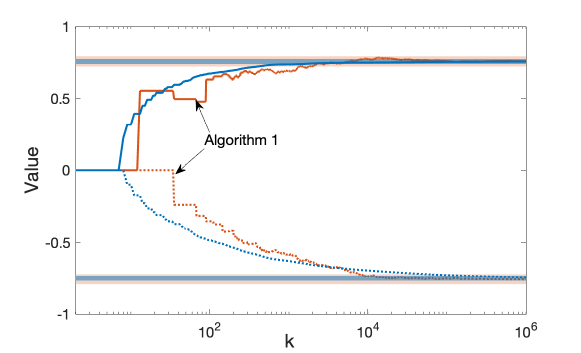
Figure 1: Evolution of the value function estimates of two agents for initial extended state in Algorithm 1 and the decentralized Q-learning dynamics presented by Sayin et al. (2021) in Scenario $1$, i.e., in two agent zero-sum MGs. Orange and blue colors are, resp., for Algorithm 1 and the other algorithm. Different line styles, i.e., solid and dotted lines, are for identifying the estimates of different agents. Shaded bars represent the error bounds, computed according to Lemma 4 without normalization.

Scenario $1$ - Two-agent Zero-sum MGs. There are two states and two actions for each state, i.e., $|S|=2$ and $|A^{i}|=2$ for $i=1,2$. The rewards are drawn randomly from the uniform distribution over $[-1,1]$ and $r^{1}(s,a)+r^{2}(s,a)=0$ for all $(s,a)$. The agents have the same discount factor $\gamma^{1}=\gamma^{2}=0.6$ and the temperature parameter is $\tau=0.01$. The underlying transition kernel is set randomly such that Assumption 4.2 holds. In this scenario, we compare the performances of Algorithm 1 with $M=11$ and the decentralized Q-learning dynamics presented by Sayin et al. (2021). The two-timescale step sizes for their algorithm are set as $\alpha_{c}=1/c^{0.9}$ and $\beta_{c}=1/c$. The former is for their local-$q$ update. Correspondingly, we use the same reference step size $\alpha_{c}=1/c^{0.9}$ for Algorithm 1. Figure 1 shows how the value function estimates for the initial state $s_{0}$ (and the initial substage $m=1$) evolve in their dynamics and Algorithm 1. Note that we can compute the unique game values for two-agent zero-sum MGs via Shapley’s iteration and they are $-0.7592$ and $0.7592$. Both algorithm reach these values approximately and the approximation error is induced by the entropy regularization. In Figure 1, we also include the error bounds on the utility $U^{i}(\pi^{i},\pi^{-i})$ induced by $\pi^{i}$’s according to Lemma 4 without the normalization. Algorithm 1 has slightly larger error bound due to (21) while achieving comparable performance with the algorithm of (Sayin et al., 2021) in two-agent zero-sum MGs. Recall that Algorithm 1 has provable convergence guarantees in a far wider range of applications, as exemplified in the following scenarios.

Figure 2: Evolution of the value function estimates of two agents for initial extended state in Algorithm 1 for different episode lengths, in Scenario $2$, i.e., MGs with a mixture of aligned and misaligned rewards. Orange and blue colors are, resp., for $M=11$ and $M=53$. Different line styles, i.e., solid and dotted lines, are for identifying the estimates of different agents. Shaded bars represent the error bounds, computed according to Lemma 4 without normalization.

Scenario $2$ - State Dependent Alignment of Rewards. There are two agents. Each agent controls an independent chain with two states, i.e., $|S^{i}|=2$ for $i=1,2$ and $|S|=|S^{1}|\cdot|S^{2}|=4$. Agents have two actions in each state, i.e., $|A^{i}|=2$ for $i=1,2$. Following (45), we set $\underline{r}^{ij}$ randomly from the uniform distribution over $[-1,1]$ and

$$\underline{r}^{ij}(s^{i},a^{i},a^{j})+\underline{r}^{ji}(s^{j},a^{j},a^{i})=0\quad\forall(a^{i},a^{j})\quad\mbox{if }s^{i}=s^{j}$$

$$\underline{r}^{ij}(s^{i},a^{i},a^{j})-\underline{r}^{ji}(s^{j},a^{j},a^{i})=0\quad\forall(a^{i},a^{j})\quad\mbox{if }s^{i}\neq s^{j}$$

$$r^{ij}(s^{j},a^{i},a^{j})+\underline{r}^{ij}(s^{i},a^{i},a^{j})=0\quad\forall(s^{i},s^{j},a^{i},a^{j}).$$

In other words, if the local states are the same, the agents receive opposite rewards, otherwise they receive identical rewards. The discount factors and temperature parameters are set as in Scenario $1$. The transition kernels for independent chains are set randomly such that Assumption 4.2 holds. The reference step size is set as in Scenario $1$, i.e., $\alpha_{c}=1/c^{0.9}$. In this scenario, we examine the performance of Algorithm 1 in certain MGs with partially (mis)aligned objectives for different episode lengths $M=11,53$. Figure 2 shows the convergent evolution of the value function estimates for the initial extended state $\underline{s}_{0}=[s_{0},0]$. Figure 2 also demonstrates the trade-off between approximation level and convergence rate when we change the episode length.

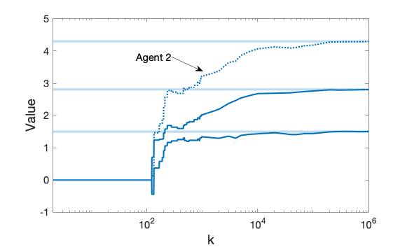
Figure 3: Evolution of the value function estimates of three agents for initial extended state in Algorithm 1 in Scenario $3$, i.e., MGs with potential stage games. Agents interact over a line network in which agent $2$ is at the center. Different line styles, i.e., solid and dotted lines, are for identifying the estimates of agent $2$. Shaded bars represent the error bounds, computed according to Lemma 4 without normalization.

Scenario $3$ - MGs with Potential Stage Games. There are three agents. Each agent controls an independent chain with two states, i.e., $|S^{i}|=2$ for each $i$ and $|S|=8$. Agents have two actions in each state, i.e., $|A^{i}|=2$ for each $i$. The pairwise interactions among agents can be represented with a line network, in which agent $2$ is at the center. Following (45) and Example 2, we set $\underline{r}^{ij}$ randomly from the uniform distribution over $[-1,1]$ and

$$r^{ij}(s^{j},a^{i},a^{j})=\underline{r}^{ji}(s^{j},a^{j},a^{i})\quad\forall(a^{i},a^{j})\quad\mbox{if }(i,j)\in E.$$

Therefore, the rewards induce a three-agent potential game for each global state. The discount factors, temperature parameters, the transition kernels, and the reference step sizes are set as in Scenario $1$. In this scenario, we examine the performance of Algorithm 1 with episode length $M=11$ in MGs with potential stage games. Figure 3 shows the convergent evolution of the value function estimates for the initial extended state $\underline{s}_{0}=[s_{0},0]$.

Note also that in Figures 1, 2, and 3, the horizontal axes are at the logarithmic scale to demonstrate the transient behavior of the algorithm. Furthermore, the vertical axes do not have identical scale. Therefore, the comparison of error bar sizes across these figures would not be fair. We plot the evolution of the iterates for a single trial rather than taking the average of multiple independent trials since the iterates might converge to different equilibria across these trials except the two-agent zero-sum case, where there is a unique game value. Lastly, the evolution of the iterates have jumps as the iterates get updated when the associated (extended) state gets visited. Correspondingly, the intervals between jumps are wider for longer episodes.

6 Conclusion

This paper introduced a decentralized learning dynamic for both time-averaged and discounted MGs with a specific focus on ARP games, as a special class of MGs. This new dynamic is radically uncoupled, model-free, rational, and convergent by reaching (near) equilibrium in two-agent zero-sum and identical-interest MGs, and certain general-sum ARP games whose rewards induce zero-sum or potential games. The approximation error is induced by the logit response and the episodic approach. The former dominates the approximation level as the latter decays with the episode length in both time-averaged and discounted cases. The paper also addressed learning in multi-agent cases for networked separable connections. Possible future research directions include addressing local state only as in (Etesami, 2023), and combining other dynamics for the repeated game scheme, such as log-linear learning (Marden et al., 2014), with Q-learning.

Appendix A Preliminary Information

Consider a sequence $\{x_{k}\in\mathbb{R}^{d}\}_{k\geq 0}$ evolving according to

$$x_{k+1}=x_{k}+\alpha_{k}(F(x_{k})+\epsilon_{k}+\omega_{k})$$ (56)

where

• The vector field $F(\cdot)$ is globally Lipshitz continuous.

• The iterates remain bounded almost surely, i.e., $\sup_{k}\|x_{k}\|_{\infty}<\infty$ with probability $1$.

• The step sizes decay, i.e., $\alpha_{k}\rightarrow 0$, at a rate such that $\sum_{k=0}^{\infty}\alpha_{k}=\infty$, and $\sum_{k=0}^{\infty}\alpha_{k}^{2}<\infty$.

• The error term $\|e_{k}\|\rightarrow 0$ with probability $1$.

• The noise term $\omega_{k}$ is a Martingale difference sequence with respect to the filtration $\mathcal{F}_{k}:=\sigma(x_{0},\omega_{0},\ldots,\omega_{k-1})$, i.e., $\mathrm{E}[\omega_{k}\mid\mathcal{F}_{k}]=0$ with probability $1$ for $k\geq 0$. Furthermore, it has finite variance conditioned on $\mathcal{F}_{k}$, i.e., $\mathrm{E}[\|\omega_{k}\|^{2}\mid\mathcal{F}_{k}]<W$ for some constant $W$.

Then, (Borkar, 2008, Chapter 2) says that $x_{k}$ almost surely converges to a compact connected internally chain transitive set of the limiting ordinary differential equation (o.d.e.)

$$\dot{x}=F(x(t))\quad\forall t\geq 0.$$ (57)

Note that the convergence of (57) does not necessarily imply the convergence of (56).

To characterize the limit behavior of (56) through (57), we follow the approach in (Benaim, 1999, Section 6.2) and call a continuously differentiable function $V:\mathbb{R}^{d}\rightarrow\mathbb{R}$ by a Lyapunov function for some compact invariant set $\Lambda\subset\mathbb{R}^{d}$ provided that for any solution to (57), we have

• $\dot{V}(x(t))<0$ for all $x(t)\notin\Lambda$

• $\dot{V}(x(t))=0$ for all $x(t)\in\Lambda$.

Then, (Benaim, 1999, Proposition 6.4) says that every internally chain transitive set of (57) is contained in $\Lambda$ provided that $V(\Lambda):=\{V(x):x\in\Lambda\}\subset\mathbb{R}$ has empty interior. Therefore, we can address the convergence of (56) by formulating such Lyapunov functions for (57). Furthermore, if $V$ is $k\geq d$ times continuously differentiable, i.e., $V\in C^{k}$, then $V(\Lambda)$ has empty interior based on Sard’s lemma (Benaim et al., 2005, Corollary 3.28).

Appendix B Technical Lemmas

This section provides the proofs of Lemmas 4, 4.1, and 4.1.

Lemma 4. Given an MG described by $\mathcal{M}=\langle S,(A^{i},r^{i})_{i=1}^{n},p,(\gamma^{i})_{i=1}^{n}\rangle$, let $(q^{j},v^{j},\pi^{j},Q^{j})$ satisfy the conditions described in (24) for each $j\in[n]$. Then, we have $U^{i}(\pi^{i},\pi^{-i})\geq U^{i}(\tilde{\pi}^{i},\pi^{-i})-\epsilon^{i}$ for any $\tilde{\pi}^{i}\in\Pi^{i}$ and each $i\in[n]$. The approximation error $\epsilon^{i}$ is given by

• for the time-averaged cases, i.e., when $\gamma^{i}=1$,

  $$\epsilon^{i}=\frac{1}{M}\times\delta^{i}+\tau\log|A^{i}|$$ (25)

• for the discounted cases, i.e., when $\gamma^{i}\in[0,1)$,

  $$\epsilon^{i}=\frac{(1-\gamma^{i})(\gamma^{i})^{M}}{1-(\gamma^{i})^{M}}\times\delta^{i}+\tau\log|A^{i}|$$ (26)

where

$$\delta^{i}:=\max_{\tilde{s}\in S}u_{0}^{M-1}(\pi^{i},\pi^{-i};\tilde{s})-\min_{\tilde{s}\in S}u_{0}^{M-1}(\pi^{i},\pi^{-i};\tilde{s})$$ (27)

and

$$u_{\underline{m}}^{\overline{m}}(\pi;s):=\mathrm{E}\left[\sum_{k=m}^{\overline{m}}(\gamma^{i})^{k-m}r^{i}(s_{k},a_{k})\mid s_{m}=s\right]$$ (28)

whose dependence on $i$ is implicit for notational simplicity and the expectation is taken with respect to the randomness on $(s_{k},a_{k})$ induced by the strategy profile $\pi$ and the underlying transition kernel.

Proof. We first evaluate the performance of $\pi^{i}$ against $\pi^{-i}$ over the episode from $k=0$ to $M-1$. To this end, let $\pi_{*}^{i}$ be an $M$-episodic strategy that is the best response to $\pi^{-i}$ for $u_{0}^{M-1}(\cdot)$, as described in (28). Then, the principle of optimality yields that

$$u_{m-1}^{M-1}(\pi_{*}^{i},\pi^{-i};s)= \;\max_{a^{i}\in A^{i}}\mathrm{E}_{a^{-i}\sim\pi^{-i}([s,m])}\bigg{[}r^{i}(s,a^{i},a^{-i})$$

$$+\gamma^{i}\sum_{s_{+}\in S}p(s_{+}\mid s,a^{i},a^{-i})u_{m}^{M-1}(\pi_{*}^{i},\pi^{-i};s_{+})\bigg{]}$$ (58)

for each $s$ and $m=1,\ldots,M-1$. For $m=M$, we have $u_{M-1}^{M-1}(\pi^{i}_{*},\pi^{-i};s)=\max_{a^{i}}\mathrm{E}[r^{i}(s,a^{i},a^{-i})]$.

By (9), the logit response $\mathrm{BR}^{i}(q^{i})$ achieves

$$0\leq\max_{a^{i}\in A^{i}}(a^{i})^{T}q^{i}-\mathrm{BR}^{i}(q^{i})^{T}q^{i}\leq\tau\log|A^{i}|=:\xi^{i}$$ (59)

for any $q^{i}\in\mathbb{R}^{|A^{i}|}$. Define $e_{m}^{i}:=\xi^{i}+\gamma^{i}e_{m+1}^{i}$ for $m<M$ and $e_{M}^{i}:=\xi^{i}$. Then, by (59), at the last stage of the episode, $m=M$, we have

$$u_{M-1}^{M-1}(\pi_{*}^{i},\pi^{-i};s)\leq v^{i}([s,M])+e_{M}^{i}.$$ (60)

For $m<M-1$, suppose that $u_{m}^{M-1}(\pi_{*}^{i},\pi^{-i};s)\leq v^{i}([s,m+1])+e_{m+1}^{i}$ for all $s$. Then, by (B), we have

$$u_{m-1}^{M-1}(\pi_{*}^{i},\pi^{-i};s)\leq \;\max_{a^{i}\in A^{i}}\mathrm{E}_{a^{-i}\sim\pi^{-i}([s,m])}\bigg{[}r^{i}(s,a^{i},a^{-i})$$

$$+\gamma^{i}\sum_{s_{+}\in S}p(s_{+}\mid s,a^{i},a^{-i})(v^{i}([s_{+},m+1])+e_{m+1}^{i})\bigg{]}$$

$$= \;\max_{a^{i}\in A^{i}}(a^{i})^{T}q^{i}([s,m],\cdot)+\gamma^{i}e_{m+1}^{i}$$ (61)

$$\leq \;v^{i}([s,m])+\xi^{i}+\gamma^{i}e_{m+1}^{i},$$ (62)

where the equality follows from (24) and the last inequality follows from (59). Therefore, we obtain $u_{m-1}^{M-1}(\pi_{*}^{i},\pi^{-i};s)\leq v^{i}([s,m])+e_{m}^{i}$ as $e_{m}^{i}=\xi^{i}+\gamma^{i}e_{m+1}^{i}$. By induction, we can conclude that

$$0\leq u_{0}^{M-1}(\pi_{*}^{i},\pi^{-i};s)-u_{0}^{M-1}(\pi^{i},\pi^{-i};s)\leq e_{0}^{i}$$ (63)

and $e_{0}^{i}$ is given by $\xi^{i}\sum_{k=0}^{M-1}(\gamma^{i})^{k}$ by its definition.

Based on (63), we next evaluate the performance of $\pi^{i}$ against $\pi^{-i}$ over the infinite horizon. Firstly, by (28), given any strategy profile $(\tilde{\pi}^{i},\pi^{-i})$, we can decompose the expected value of the discounted sum of the rewards as

$$u_{0}^{LM-1}(\tilde{\pi}^{i},\pi^{-i};s_{0})=u_{0}^{M-1}(\tilde{\pi}^{i},\pi^{-i};s_{0})+\sum_{\ell=1}^{L-1}(\gamma^{i})^{M\ell}\mathrm{E}[u_{M\ell}^{M(\ell+1)-1}(\tilde{\pi}^{i},\pi^{-i};s_{M\ell})]$$ (64)

for any $L=1,2,\ldots$, where the expectations on the right-hand side are taken with respect to the randomness on $s_{M\ell}$. Note that $\pi^{-i}$ are $M$-episodic strategies though $\tilde{\pi}^{i}$ can be any strategy from $\Pi$. Since the $M$-episodic strategy $\pi_{*}^{i}$ is the best response to $\pi^{-i}$ for $u_{0}^{M-1}(\cdot)$, the decomposition yields that

$$\max_{\tilde{\pi}^{i}}u_{0}^{LM-1}(\tilde{\pi}^{i},\pi^{-i};s_{0})\leq u_{0}^{M-1}(\pi_{*}^{i},\pi^{-i};s_{0})+\max_{\tilde{s}\in S}u_{0}^{M-1}(\pi^{i}_{*},\pi^{-i};\tilde{s})\times\sum_{\ell=1}^{L-1}(\gamma^{i})^{M\ell},$$ (65)

where we use the fact that $u_{M\ell}^{M(\ell+1)-1}(\pi^{i}_{*},\pi^{-i};\tilde{s})=u_{0}^{M-1}(\pi^{i}_{*},\pi^{-i};\tilde{s})$ for all $\ell$ as the strategies are $M$-episodic. Correspondingly, by (63), we obtain the upper bound:

$$\max_{\tilde{\pi}^{i}}u_{0}^{LM-1}(\tilde{\pi}^{i},\pi^{-i};s_{0})\leq u_{0}^{M-1}(\pi^{i},\pi^{-i};s_{0})+\max_{\tilde{s}\in S}u_{0}^{M-1}(\pi^{i},\pi^{-i};\tilde{s})\times\sum_{\ell=1}^{L-1}(\gamma^{i})^{M\ell}+e_{0}^{i}\sum_{\ell=0}^{L-1}(\gamma^{i})^{M\ell}.$$

Correspondingly, we also obtain the lower bound:

$$\max_{\tilde{\pi}^{i}}u_{0}^{LM-1}(\tilde{\pi}^{i},\pi^{-i};s_{0}) \geq u_{0}^{LM-1}(\pi^{i},\pi^{-i};s_{0})$$

$$\geq u_{0}^{M-1}(\pi^{i},\pi^{-i};s_{0})+\min_{\tilde{s}\in S}u_{0}^{M-1}(\pi^{i},\pi^{-i};\tilde{s})\times\sum_{\ell=1}^{L-1}(\gamma^{i})^{M\ell},$$

where the last inequality follows from (64). The upper and the lower bounds computed above yield that

$$\max_{\tilde{\pi}^{i}}u_{0}^{LM-1}(\tilde{\pi}^{i},\pi^{-i};s_{0})-u_{0}^{LM-1}(\pi^{i},\pi^{-i};s_{0})\leq\delta^{i}\sum_{\ell=1}^{L-1}(\gamma^{i})^{M\ell}+e_{0}^{i}\sum_{\ell=0}^{L-1}(\gamma^{i})^{M\ell},$$ (66)

where the right-hand side is the distance between the upper and lower bounds and $\delta^{i}$ is as described in (27).

By (3) and (28), we can write the agent $i$’s utility as

$$U^{i}(\pi^{i},\pi^{-i})=\lim_{L\rightarrow\infty}\frac{1}{\sum_{k=0}^{LM-1}(\gamma^{i})^{k}}\mathrm{E}[u_{0}^{LM-1}(\pi^{i},\pi^{-i};s)],$$

where the expectation is taken over $s\sim p_{o}\in\Delta(S)$ that is the initial state distribution. Therefore, in the time-averaged case, i.e., when $\gamma^{i}=1$, we obtain

$$\sup_{\tilde{\pi}^{i}}U^{i}(\tilde{\pi}^{i},\pi^{-i})-U^{i}(\pi^{i},\pi^{-i})\leq\delta^{i}\frac{1}{M}+e_{0}^{i}\frac{1}{M}.$$ (67)

On the other hand, in the discounted case, i.e., when $\gamma^{i}\in[0,1)$, (66) yields that

$$\max_{\tilde{\pi}^{i}}U^{i}(\tilde{\pi}^{i},\pi^{-i})-U^{i}(\pi^{i},\pi^{-i})\leq\delta^{i}\frac{(1-\gamma^{i})(\gamma^{i})^{M}}{1-(\gamma^{i})^{M}}+e_{0}^{i}\frac{1-\gamma^{i}}{1-(\gamma^{i})^{M}}.$$ (68)

Recall that $e_{0}^{i}=\xi^{i}\sum_{k=0}^{M-1}(\gamma^{i})^{k}$. In the time-averaged case, $e_{0}^{i}=\xi M$ and the error induced by the smoothed best response is $e_{0}^{i}/M=\xi^{i}$. In the discounted case, $e_{0}^{i}=\xi^{i}(1-(\gamma^{i})^{M})/(1-\gamma^{i})$ and the error is given by $e_{0}^{i}(1-\gamma^{i})/(1-(\gamma^{i})^{M})=\xi^{i}$. This completes the proof. $\square$

Lemma 4.1. The candidate $\dot{V}_{z}(q,\underline{q},\pi)\leq 0$ for all $(q,\underline{q},\pi)$ and $\dot{V}_{z}(q,\underline{q},\pi)=0$ if and only if $V_{z}(q,\underline{q},\pi)=0$.

Proof. Since $L_{z}(\cdot)$ is continuously differentiable due to the smoothness induced by the entropy regularization, we can apply the envelope theorem and chain rule to compute its time derivative as

$$\frac{dL_{z}(\underline{q},\pi)}{dt} =\sum_{i=1}^{n}\left((\mathrm{br}^{i})^{T}\left(\hat{\underline{q}}^{i}-q^{i}\right)-\tau\nabla H^{i}(\pi^{i})\cdot\dot{\pi}^{i}\right)$$

$$=-\sum_{i=1}^{n}\left((\mathrm{br}^{i})^{T}\underline{q}^{i}+\tau\nabla H^{i}(\pi^{i})\cdot\dot{\pi}^{i}\right),$$ (69)

which follows from $\sum_{i=1}^{n}(\mathrm{br}^{i})^{T}\sum_{j:(i,j)\in E}\underline{U}^{ij}\mathrm{br}^{j}=0$. Since $\sum_{i=1}^{n}(\pi^{i})^{T}\bar{\underline{q}}^{i}=0$, by adding and subtracting $\tau H^{i}(\mathrm{br}^{i})$’s and $\tau H^{i}(\pi^{i})$’s to (69), we obtain

$$\frac{dL_{z}(\underline{q},\pi)}{dt}= \;-\sum_{i=1}^{n}((\mathrm{br}^{i}-\pi^{i})^{T}\underline{q}^{i}+\tau H^{i}(\mathrm{br}^{i})-\tau H^{i}(\pi^{i}))$$

$$+\tau\sum_{i=1}^{n}(H^{i}(\mathrm{br}^{i})-H^{i}(\pi^{i})-\nabla H^{i}(\pi^{i})\cdot(\mathrm{br}^{i}-\pi^{i}))-\sum_{i=1}^{n}(\pi^{i})^{T}\left(\underline{q}^{i}-\bar{\underline{q}}^{i}\right).$$ (70)

The first summation on the right-hand side of (70) corresponds to $L_{z}(\underline{q},\pi)$. The second summation is non-positive since $H^{i}(\mathrm{br}^{i})-H^{i}(\pi^{i})\leq\nabla H^{i}(\pi^{i})(\mathrm{br}^{i}-\pi^{i})$ due to the concavity of the entropy function $H^{i}(\cdot)$. Therefore, we obtain

$$\dot{L}_{z}\leq-L_{z}-\sum_{i=1}^{n}(\pi^{i})^{T}\left(\underline{q}^{i}-\bar{\underline{q}}^{i}\right).$$ (71)

On the other hand, the time derivatives of $\underline{M}(\underline{q},\pi)$ and $M(q,\pi)$ are, resp., given by $\dot{\underline{M}}=-\underline{M}$ and $\dot{M}=-M$. Note that $-(\pi^{i})^{T}\left(\underline{q}^{i}-\bar{\underline{q}}^{i}\right)\leq\left\|\underline{q}^{i}-\bar{\underline{q}}^{i}\right\|_{\infty}$ since $\pi^{i}$ is a probability distribution. Therefore, we obtain

$$\dot{V}_{z}=\dot{L}_{z}+2\dot{\underline{M}}+\dot{M}\leq-L_{z}-\underline{M}-M,$$

where the inequality follows from (71) and $\left\|\underline{q}^{i}-\bar{\underline{q}}^{i}\right\|_{\infty}\leq\left\|\underline{q}^{i}-\bar{\underline{q}}^{i}\right\|_{2}=M$.

Note that $L_{z}(\underline{q},\pi)\geq 0$ for all $(\pi^{i}\in\Delta(A^{i}))_{i=1}^{n}$ and $\underline{M}(\cdot)$, $M(\cdot)$ are non-negative by definition (44). Therefore, we have $\dot{V}_{z}(\underline{q},\pi)\leq 0$ for all $(\underline{q},\pi)$ and $\dot{V}(\underline{q},\pi)=0$ if and only if the non-negative functions $L_{z}(\underline{q},\pi)$, $\underline{M}(\underline{q},\pi)$ and $M(q,\pi)$ are all zero, and therefore, $V_{z}(q,\underline{q},\pi)=0$. $\square$

Lemma 4.1. The candidate $\dot{V}_{p}(q,\underline{q},\pi)\leq 0$ for all $(q,\underline{q},\pi)$ and $\dot{V}_{z}(q,\underline{q},\pi)=0$ if and only if $(q,\underline{q},\pi)\in\Lambda_{p}$, defined by $\Lambda_{p}:=\{(q,\underline{q},\pi):\;q^{i}=\hat{q}^{i},\;\underline{q}^{i}=\hat{\underline{q}}^{i},\pi^{i}=\mathrm{BR}^{i}(\hat{q}^{i})\}$.

Proof. Again the envelope theorem and the chain rule yield that the time derivative of $L_{p}$ is given by

$$\frac{dL_{p}(\pi)}{dt} =\sum_{i=1}^{n}\left((\dot{\pi}^{i})^{T}\left(\sum_{j:(i,j)\in E}\Phi^{ij}\pi^{j}\right)+\tau\nabla H^{i}(\pi^{i})\dot{\pi}^{i}\right)$$

$$\stackrel{{\scriptstyle(a)}}{{=}}\sum_{i=1}^{n}\left((\mathrm{br}^{i}-\pi^{i})^{T}\bar{\underline{q}}^{i}+\tau\nabla H^{i}(\pi^{i})(\mathrm{br}^{i}-\pi^{i})\right)$$

$$\stackrel{{\scriptstyle(b)}}{{=}}\sum_{i=1}^{n}\left((\mathrm{br}^{i}-\pi^{i})^{T}\underline{q}^{i}+\tau H^{i}(\mathrm{br}^{i})-\tau H^{i}(\pi^{i})\right)-\tau\sum_{i=1}^{n}\left(H^{i}(\mathrm{br}^{i})-H^{i}(\pi^{i})-\nabla H^{i}(\pi^{i})(\mathrm{br}^{i}-\pi^{i})\right)$$

$$\hskip 7.22743pt-\sum_{i=1}^{n}(\mathrm{br}^{i}-\pi^{i})^{T}\left(\underline{q}^{i}-\bar{\underline{q}}^{i}\right),$$ (72)

where $(a)$ follows from (34) and the definition of $\bar{\underline{q}}^{i}$; $(b)$ follows from adding and subtracting $(\dot{\pi}^{i})^{T}\underline{q}^{i}$, $\tau H^{i}(\mathrm{br}^{i})$ and $\tau H^{i}(\pi^{i})$ for each $i\in[n]$.

Note that $-(\mathrm{br}^{i}-\pi^{i})^{T}\left(\underline{q}^{i}-\bar{\underline{q}}^{i}\right)\leq 2\left\|\underline{q}^{i}-\bar{\underline{q}}^{i}\right\|_{\infty}\leq 2\underline{M}$ since $\mathrm{br}^{i}$ and $\pi^{i}$ are probability distributions. Since $\dot{\underline{M}}=-\underline{M}$ and $\dot{M}=-M$, we have

$$\dot{V}_{p} \leq-\sum_{i=1}^{n}\left((\mathrm{br}^{i}-\pi^{i})^{T}\underline{q}^{i}+\tau H^{i}(\mathrm{br}^{i})-\tau H^{i}(\pi^{i})\right)+\tau\sum_{i=1}^{n}\left(H^{i}(\mathrm{br}^{i})-H^{i}(\pi^{i})-\nabla H^{i}(\pi^{i})(\mathrm{br}^{i}-\pi^{i})\right)$$

$$\hskip 7.22743pt-\underline{M}-M$$ (73)

which follows from (44) and the fact that $\|x\|_{2}\geq\|x\|_{\infty}$ for any vector $x$. The first and second summations on the right-hand side are non-positive, resp., by $\mathrm{br}^{i}=\mathrm{BR}^{i}(\underline{q}^{i})$ and the concavity of the entropy regularization. This implies that each term in the upper bound (73) are non-positive. Therefore, $\dot{V}_{p}(q,\underline{q},\pi)\leq 0$ for all $(q,\underline{q},\pi)$ and $\dot{V}_{p}=0$ if and only if these terms are all zero, which is the case if and only if $(q,\underline{q},p)\in\Lambda_{p}$. $\square$

References

• Arslan and Yüksel [2017] G. Arslan and S. Yüksel. Decentralized Q-learning in stochastic teams and games. IEEE Transactions on Automatic Control, 62(4), 2017.
• Arslan et al. [2007] G. Arslan, M. F. Demirkol, and Y. Song. Equilibrium efficiency improvement in MIMO interference systems: A decentralized stream control approach. IEEE Transactions on Wireless Communications, 6(8):2984–2993, 2007.
• Başar [1986] T. Başar. Dynamic Games and Applications in Economics, volume 265. Springer Science & Business Media, 1986.
• Başar and Olsder [1998] T. Başar and G. J. Olsder. Dynamic Noncooperative Game Theory. Society for Industrial and Applied Mathematics (SIAM), 1998.
• Baudin and Laraki [2022] L. Baudin and R. Laraki. Best-response dynamics and fictitious play in identical interest stochastic games. In Proc. Internat. Conf. Machine Learn. (ICML), pages 1664–1690, 2022.
• Benaim [1999] M. Benaim. Dynamics of stochastic approximation algorithms. In Le Seminaire de Probabilities, Lecture Notes in Math. 1709, pages 1–68, Berlin, 1999. Springer-Verlag.
• Benaim et al. [2005] M. Benaim, J. Hofbauer, and S. Sorin. Stochastic approximations and differential inclusions. SIAM Journal on Control and Optimization, 44(1):328–348, 2005.
• Blackwell and Ferguson [1968] D. Blackwell and T. S. Ferguson. The big match. Ann. Math. Statist., 39:159–163, 1968.
• Borkar [2008] V. S. Borkar. Stochastic Approximation: A Dynamical Systems Viewpoint. Hindustan Book Agency, 2008.
• Cai et al. [2016] Y. Cai, O. Candogan, C. Daskalakis, and C. Papadimitriou. Zero-sum polymatrix games: A generalization of minimax. Mathematics of Operations Research, 41(2):648–655, 2016.
• Ding et al. [2022] D. Ding, C.-Y. Wei, K. Zhang, and M. R. Jovanovic. Independent policy gradient for large-scale Markov potential games: Sharper rates, function approximation, and game-agnostic convergence. In Proc. Internat. Conf. Machine Learn. (ICML), 2022.
• Eldosouky et al. [2016] A. Eldosouky, W. Saad, and D. Niyato. Single controller stochastic games for optimized moving target defense. In Proc. IEEE Internat. Conf. Communications, 2016.
• Etesami [2023] S. R. Etesami. Learning stationary Nash equilibrium policies in n-player stochastic games with independent chains. arXiv preprint arXiv:2201.12224, 2023.
• Filar and Vrieze [1997] J. Filar and K. Vrieze. Competitive Markov Decision Processes. Springer, 1997.
• Fink [1964] A. M. Fink. Equilibrium in stochastic n-person game. Journal of Science Hiroshima University Series A-I, 28:89–93, 1964.
• Flesch et al. [2008] J. Flesch, G. Schoenmakers, and K. Vrieze. Stochastic games on a product state space. Mathematics of Operations Research, 33(2):403–420, 2008.
• Gillette [1957] D. Gillette. Stochastic games with zero stop probabilities. In M. Dresher, A. W. Tucker, and P. Wolfe, editors, Contributions to the Theory of Games, volume III of Ann. Math. Stud., pages 179–187. Princeton University Press, Princeton, NJ, 1957.
• Hofbauer and Hopkins [2005] J. Hofbauer and E. Hopkins. Learning in perturbed asymmetric games. Games and Economic Behavior, 52:133–152, 2005.
• Hofbauer and Sandholm [2002] J. Hofbauer and W. H. Sandholm. On the global convergence of stochastic fictitious play. Econometrica, 70:2265–2294, 2002.
• Jin et al. [2021] C. Jin, Q. Liu, Y. Wang, and T. Yu. V-learning - A simple, efficient, decentralized algorithm for multiagent rl. arXiv preprint arXiv:2110.14555, 2021.
• Kalogiannis and Panageas [2023] F. Kalogiannis and I. Panageas. Zero-sum polymatrix Markov games: Equilibrium collapse and efficient computation of Nash equilibria. arXiv preprint arXiv:2305.14329, 2023.
• Leonardos et al. [2022] S. Leonardos, W. Overman, and I. Panageas ans G. Piliouras. Global convergence of multi-agent policy gradient in Markov potential games. In International Conference on Learning Representations, 2022.
• Leslie and Collins [2005] D. S. Leslie and E. J. Collins. Individual Q-learning in normal form games. SIAM J. Control Optim., 44(2):495–514, 2005.
• Leslie et al. [2020] D. S. Leslie, S. Perkins, and Z. Xu. Best-response dynamics in zero-sum stochastic games. Journal of Economic Theory, 189, 2020.
• Littman [1994] M. L. Littman. Markov games as a framework for multi-agent reinforcement learning. In Proceedings of the 11th International Conference on Machine Learning (ICML), 1994.
• Mao and Başar [2022] W. Mao and T. Başar. Provably efficient reinforcement learning in decentralized general-sum Markov games. Dynamic Games and Applications, 13:165–186, 2022.
• Marden et al. [2014] J. R. Marden, H. P. Young, and L. Y. Pao. Achieving Pareto optimality through distributed learning. SIAM Journal on Control and Optimization, 52(5):2753–2770, 2014.
• McKelvey and Palfrey [1995] R. McKelvey and T. Palfrey. Quantal response equilibria for normal form games. Games and Economic Behavior, 10:6–38, 1995.
• Park et al. [2023] C. Park, K. Zhang, and A. Ozdaglar. Multi-player zero-sum Markov games with networked separable interactions. arXiv preprint arXiv:2307.09470, 2023.
• Parthasaranthy and Raghavan [1981] T. Parthasaranthy and T. Raghavan. An orderfield property for stochastic games when one player controls transition probabilities. Journal of Optimization Theory and Applications, 33(3):375–392, 1981.
• Perolat et al. [2018] J. Perolat, B. Piot, and O. Pietquin. Actor-critic fictitious play in simultaneous move multistage games. In Proceedings of the 21st International Conference on Artificial Intelligence and Statistics (AISTATS), 2018.
• Sayin [2022] M. O. Sayin. Global convergence of stochastic fictitious play in stochastic games with turn-based controllers. arXiv preprint arXiv:2204.01382, 2022.
• Sayin et al. [2021] M. O. Sayin, K. Zhang, D. S. Leslie, A. Ozdaglar, and T. Başar. Decentralized Q-learning in zero-sum Markov games. In Advances in Neural Information Processing, 2021.
• Sayin et al. [2022a] M. O. Sayin, F. Parise, and A. Ozdaglar. Fictitious play in zero-sum stochastic games. SIAM Journal on Control and Optimization, 60(4):2095–2114, 2022a. doi: 10.1137/21M1426675.
• Sayin et al. [2022b] M. O. Sayin, K. Zhang, and A. Ozdaglar. Fictitious play in Markov games with single controller. In ACM Conference on Economics and Computation (EC), pages 919–936, 2022b. ISBN 9781450391504.
• Shapley [1953] L. S. Shapley. Stochastic games. Proceedings of National Academy of Science USA, 39(10):1095–1100, 1953.
• Song et al. [2022] Z. Song, S. Mei, and Y. Bai. When can we learn general-sum Markov games with a large number of players sample-efficiently? In Proc. Internat. Conf. Learning Representations, 2022.
• Wei et al. [2021] C.-Y. Wei, C.-W. Lee, M. Zhang, and H. Luo. Last-iterate convergence of decentralized optimistic gradient descent/ascent in infinite-horizon competitive markov games. In M. Belkin and S. Kpotufe, editors, 34th Annual Conference on Learning Theory, volume 134, pages 1–41, 2021.
• Xu et al. [2012] Y. Xu, J. Wang, Q. Wu, A. Anpalagan, and Y. D. Yao. Opportunistic spectrum access in cognitive radio networks: Global optimization using local interaction games. IEEEJournal of Selected Topics in Signal Processing, 6(2):180–194, 2012.
• Zhang et al. [2021] K. Zhang, Z. Yang, and T. Başar. Multi-agent reinforcement learning: A selective overview of theories and algorithms. In K. G. Vamvoudakis, Y. Wan, F. L. Lewis, and D. Cansever, editors, Handbook on RL and Control, volume 325 of Studies in Systems, Decision and Control. Springer, Cham, 2021.
• Zhang et al. [2022] R. Zhang, Z. Ren, and N. Li. Gradient play in stochastic games: Stationary points and local geometry. In Proc. IFAC PapersOnLine, 2022.
• Zheng et al. [2014] J. Zheng, Y. Cai, Y. Liu, Y. Xu, B. Duan, and X. Shen. Optimal power allocation and user scheduling in multicell networks: Base station cooperation using a game-theoretic approach. IEEE Transactions on Wireless Communications, 13(12):6928–6942, 2014.