Input-Output Relation and Low-Complexity Receiver Design for CP-OTFS Systems with Doppler Squint
Xuehan Wang1, Xu Shi1, Jintao Wang1,2, Jian Song1,2,3 This work was supported in part by Tsinghua University-China Mobile Research Institute Joint Innovation Center.
1Beijing National Research Center for Information Science and Technology (BNRist),
Dept. of Electronic Engineering, Tsinghua University, Beijing, China
2Research Institute of Tsinghua University in Shenzhen, Shenzhen, China
3Shenzhen International Graduate School, Tsinghua University, Shenzhen, Guangdong, 518055
{wang-xh21@mails., shi-x19@mails., wangjintao@, jsong@}tsinghua.edu.cn
Abstract
In orthogonal time frequency space (OTFS) systems, the impact of frequency-dependent Doppler which is referred to as the Doppler squint effect (DSE) is accumulated through longer duration, whose negligence has prevented OTFS systems from exploiting the performance superiority. In this paper, practical OFDM system using cyclic prefix time guard interval (CP-OFDM)-based OTFS systems with DSE are adopted. Cyclic prefix (CP) length is analyzed while the input-output relation considering DSE is derived. By deploying two prefix OFDM symbols, the channel estimation can be easily divided into three parts as delay detection, Doppler extraction and gain estimation. The linear equalization scheme is adopted taking the block diagonal property of the channel matrix into account, which completes the low-complexity receiver design. Simulation results confirm the significance of DSE and the considerable performance of the proposed low-complexity receiver scheme considering DSE.
Reliable data transmission in high-mobility scenarios where the velocity approaches km/h is regarded as one of the key requirements in the 6G mobile network [1], where orthogonal time frequency space (OTFS) modulation is becoming a promising alternative to generate the communication waveform. By placing data symbols in delay-Doppler grids, the doubly-selective fading caused by the high-mobility and multipath propagation can be easily mitigated since full diversity over time-frequency is utilized for each symbol. So far, extensive work has verified the performance superiority of OTFS compared with traditional schemes such as orthogonal frequency-division multiplexing (OFDM) [2, 3].
For practical OTFS systems, linear minimum mean squared error (LMMSE)-based equalizer can satisfactorily address the trade-off between the complexity and reliability [4, 5]. However, the attainment of channel state information (CSI) remains an open problem and has drawn substantial attention [6, 7, 8, 9]. Threshold-based delay-Doppler detection was developed, where the threshold can be fixed [6] or adaptive [7]. Meanwhile, compressed sensing-based schemes usually outperform the threshold-based methods by exploiting the sparsity of parameters, e.g., the Bayesian approaches [8, 9].
However, the subcarrier-dependent Doppler which is referred to as the Doppler squint effect (DSE) exists and the deviation is accumulated through much longer duration in OTFS systems, which leads to severe performance degradation [10] in most of existing schemes [2, 3, 4, 5, 6, 7, 8, 9, 11, 12] due to the fundamental input-output analysis [11, 12] ignoring DSE. To the best of the authors’ knowledge, [10] is the only work considering DSE. However, impractical waveform and low transmission efficiency are involved, which inspires more efficient and practical design for OTFS systems with DSE.
In this paper, OFDM system using cyclic prefix time guard interval (CP-OFDM)-based OTFS is adopted. The input-output relation is analyzed based on the multipath linear time-variant (LTV) model with DSE, where the cyclic prefix (CP) length is elaborately designed to ensure no inter-symbol interference (ISI) between OFDM symbols within an OTFS symbol. The low-complexity receiver is then provided, where channel parameters are recovered by delay detection, Doppler extraction and gain estimation while the LMMSE-based equalizer is employed for each OFDM symbol. Finally, simulation results confirm the significance of DSE and the excellent performance of the proposed low-complexity receiver considering DSE.
Notations: , , denote a matrix, column vector and scalar, respectively. and are its conjugate transposition and inverse. denotes the Frobenius-norm of . represents the ceiling function while denotes the modulus operation with respect to . returns the average value of . Finally, returns the phase of complex value .
II System Model
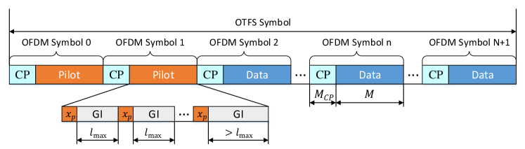
CP-OFDM-based OTFS system [9] with the frame structure in Fig. 1 is investigated in this section. The multipath LTV channel with DSE is also presented, where we analyze why it cannot be ignored in OTFS systems. and denote the carrier frequency and subcarrier spacing, respectively. The impact of noise is disregarded for ease of illustration.
II-AOTFS Transmitter and Frame Structure
At the transmitter, information bits are mapped to symbols as on the delay-Doppler grid. are then converted to time-frequency symbols employing the inverse symplectic finite Fourier transform (ISFFT). Let and denote the maximum delay and Doppler spread corresponding to , where we have and .
Figure 1: OTFS frame structure in the time domain.
CP-OFDM is adopted as the pulse-shape to create the continuous baseband waveform. and represent the time duration of a CP and an entire OFDM symbol, where we have to guarantee the orthogonality. OTFS frame structure in the time domain is depicted in Fig. 1, where two prefix OFDM symbols are allocated for channel estimation. Let denote time-frequency symbols including the pilot and data which is loaded as . The transmitted waveform in the time domain can be derived as
Let and represent the pilot value and the number of pilots within an OFDM symbol, where we have
(3)
for . When it comes to OFDM symbols where data is loaded, we can derive
(4)
II-BMultipath LTV Channel Model with DSE
The passband waveform travels from the transmitter to the receiver via incident paths. The received passband signal is [13, 10]
(5)
where and represent the velocity with which the path length decreases and the speed of light, respectively. , denote the attenuation and propagation delay of the path, respectively. Let denote the Doppler shift at and remove the carrier , the baseband received signal can be written as
(6)
For OFDM systems, the frame duration is while the sampling period is , which deduces even though in high-mobility scenarios with large number of subcarriers, e.g., km/h and . Therefore, holds true, which derives the channel model employed in [11]. However, in OTFS systems, the frame duration becomes longer than . Meanwhile, is usually large to enjoy full-time diversity, e.g., [11, 8]. Therefore, is about for , and km/h, which is non-negligible.
On the other hand, the time-variant frequency response is also widely employed to characterize the LTV channel. The received signal can be derived [10] as , where is the Fourier transform of . Combining with (6), can be derived as
(7)
where we have to simplify the notation. (7) indicates that the Doppler shift brought by the high-mobility in multipath LTV channel is , which is frequency-dependent and referred to as DSE. In OTFS systems, the subcarrier-dependent phase offset brought by DSE will be accumulated within one OTFS symbol as . Taking the typical value as , and km/h, DSE leads to a maximum offset about , which plays a significant role in OTFS systems. If ignored directly, striking performance degradation occurs [10].
Moreover, DSE leads to time-frequency coupling and destroys the sparsity in delay-Doppler channel response, which is disastrous to most of existing designs since the sparsity of the delay-Doppler channel is usually treated as the basic assumption. According to [10], the delay-Doppler response of multipath LTV channel for is , where we have for ease of illustration. It is significantly different from the channel model in [11, 12], which inspires us to reconsider the input-output analysis and receiver design in prior work for practical OTFS systems with DSE.
III OTFS Input-Output Analysis with DSE
At the receiver, is sampled as like . In this section, we investigate the CP length to ensure no ISI between OFDM symbols and derive the input-output relation with DSE. Meanwhile, notations and are employed, where is required to exploit the delay resolution. Similar to [10], OTFS system with is adopted in this paper, which is easily compatible with the existing wireless communication network [11], e.g., , with the relative velocity km/h.
III-ARequirement of CP Length
In order to simplify the equalization by employing the block diagonal property of channel matrix like [5, 14], CP length is required to be adequate to confirm no ISI between OFDM symbols, which is illustrated in detail in this subsection.
Combining (6) with (1) at the sampled point, the requirement of CP length is
(8)
which is obtained from the duration of . Let us begin with the analysis of the left part, where (8) can be simplified as
(9)
By employing , we have
(10)
where (a) is attained by assuming .
(10) means is sufficient to ensure (9).
On the other hand, we can derive
(11)
where (a) is obtained by employing and . (11) indicates that no additional conditions are demanded to achieve (8). Therefore, if the length of CP satisfies
(12)
there will be no ISI between OFDM symbols, which simplifies the receiver design significantly.
III-BOTFS Input-Output Analysis with DSE
In this subsection, the input-output analysis is offered, where the CP length satisfies (12). The relation between and is provided by the following theorem.
Theorem 1.
The input-output relation of CP-OFDM-based OTFS systems can be represented as
Compared with prior analysis in [9] where is treated as to ignore DSE, two modifications occur in (14):
1)
Delay spread extension: If in the phase of sinc function is ignored, holds true for when integer delay is involved. However, extra phase destroys this property and brings more delay spread. Though the location of the most powerful channel coefficient seldom changes due to DSE, significant delay spread extension aggravates the interference within an OFDM symbol especially when is large.
2)
Extra phase shift: DSE introduces an extra phase shift besides traditional Doppler shift, which is represented as
(15)
Taking the typical value as , , and the relative velocity as km/h, DSE leads to a maximum phase offset of about .
From the analysis above, the significance of DSE is determined by , which can be approximately measured by . It is different from prior declaration [15] where DSE is caused only by large bandwidth. Since the Doppler squint accumulates through the time, the significance is determined by the size of the entire time-frequency block rather than the bandwidth. e.g., if the bandwidth is fixed, more subcarriers mean smaller subcarrier spacing, which increases and consequently amplifies the significance of DSE. As a result, the impact of DSE is dependent on the ratio between the time-frequency resource block size and the mobility parameter .
Meanwhile, DSE disappears when , whose input-output formulation can be treated as the limit for (14) when . It is worth pointing out that the delay-Doppler input-output relationship can also be attained by Theorem 1. However, it is not depicted since no closed-form representation can be achieved and the derivation cannot benefit the receiver design in this paper. It is also valuable to focus on the delay-Doppler response and provide the corresponding receiver schemes, where similar characteristics appear like [10].
IV Low-Complexity Receiver Design with DSE
In this section, the low-complexity OTFS receiver design including the parameter extraction-based channel recovery and the LMMSE-based data detection is illustrated in detail. Similar to [8, 5, 6, 7, 9, 11, 10], the system bandwidth is assumed to be sufficient to eliminate the fractional delay, where are all integers while are not necessarily integers.
IV-AChannel Estimation Scheme
At first, can be derived for OFDM symbols employed for channel estimation since , and hold true. It indicates that the phase of sinc function in (14) can be approximated by . Therefore, if there is not a path with delay , we can deduce
(16)
Otherwise, the received symbols can be represented as
(17)
for if there is a path with , and , which inspires us to judge the existence of path with by employing the threshold-based detection. We employ the vectorized notation as for . for indicates there is a path with delay .
After detecting the path with , can be extracted by phase differences. Let denote the phase difference array which is computed as
(18)
If ignoring the noise, holds true, which motivates the approximate extraction of as
(19)
Finally, the least-square (LS) solution is employed to estimate , where the base vector are
(20)
for . can be easily attained by
(21)
where . After the parameter extraction of , and , CSI can be recovered by Theorem 1.
IV-BLMMSE-based Equalization Scheme
Algorithm 1 Proposed OTFS Receiver design with DSE
0: , , , , and .
1:Channel Estimation:
2:Initialize , and as empty parameter vectors;
3:fordo
4: Generate and by ;
5: % Detect the path with delay
6:ifthen
7: Successfully detect the path with delay ;
8: Extract the normalized Doppler by (18) and (19);
Since no ISI between OFDM symbols is introduced, it is much easier to carry out the equalization for each OFDM symbol. The vectorized input-output relationship is employed as , where we have , and . denotes the additive white Gaussian noise.
The LMMSE-based equalizer is then implemented as
(22)
where are recovered as based on the estimated parameters. represents the average power of , which is deduced by employing the property of IFFT in (4). Delay-Doppler symbols can therefore be recovered by
(23)
which can be directly employed to recover information bits.
IV-CLow-Complexity Receiver Design
The low-complexity OTFS receiver design with DSE is briefly drawn in this subsection. As illustrated in Algorithm 1, the parameter estimation-based CSI recovery is carried out first, which can be divided into three steps as delay detection, Doppler extraction and gain estimation. The estimated parameters are then employed to recover the channel matrices , which are utilized in the LMMSE-based equalizer. At last, delay-Doppler symbols can be estimated and information bits can be obtained, which finishes the design of OTFS receiver considering DSE.
For each iteration of channel estimation, the computational complexity is bounded as , which causes a total load of for the parameter extraction. When it comes to the data detection, complexity of is required due to the inversion operation in each iteration. Taking the excellent structure for parallel processing in Algorithm 1, the total complexity can be bounded as , which is quite lower than the delay-Doppler implementation of LMMSE-based receiver with . It is worth pointing out that though plenty of works have been devoted to the LMMSE-based receiver [4, 5] with lower complexity, the negligence of DSE leads to the failure of these schemes, which inspires future work to further explore the channel structure of DSE and develop more efficient receiver designs.
V Simulation Results
TABLE I: Simulation Parameters
Parameter
Typical value
Carrier frequency ()
GHz
Subcarrier spacing ()
kHz
Number of subcarriers ()
1024
Number of OFDM symbols ()
128
UE speed (km/h)
1000
Number of paths ()
4
Maximum delay grid ()
20
Length of CP ()
24
Modulation alphabet
QPSK
The significance of DSE and the performance of the proposed receiver scheme are evaluated in this section by presenting simulation results. Jakes’ formula is utilized to generate the Doppler shift of each path as where is uniformly distributed over . Complex coefficients are generated as . The normalized mean squared error (NMSE) of the channel matrix is defined as
(24)
which is employed to evaluate the error of both the model and the estimation. We set and limit the absolute value of by to implement Algorithm 1. The system signal-to-noise ratio is defined as SNR while the power of pilot symbols is 30dB higher than .
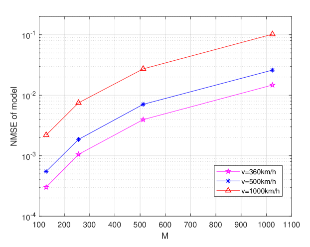
Figure 2: NMSE against with perfect knowledge of channel parameters.
The significance of DSE is first verified by plotting NMSE of model in Fig. 2, where in (24) denotes the channel matrix ignoring DSE with perfect knowledge of parameters. It is clear that the impact of DSE increases with the velocity and increasing. NMSE of about 10% occurs when km/h and , which deserves serious consideration to ensure the reliability in practical OTFS systems.
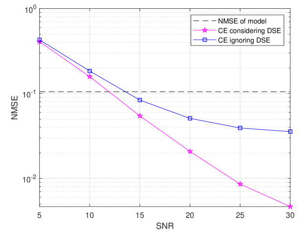
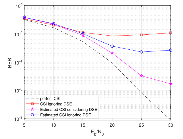
Figure 3: NMSE performance against SNR with parameters set as Table I.Figure 4: BER performance against SNR with parameters set as Table I.
Fig. 3 demonstrates the performance of channel estimation by presenting the NMSE comparison. When SNRdB, NMSE of the estimated CSI considering DSE approaches half of NMSE of model. NMSE of estimated CSI considering DSE is less than when SNRdB. However, NMSE is more than when SNRdB if neglecting DSE, which confirms the importance of considering DSE again.
(25)
In Fig. 4, BER comparison is displayed to show the performance superiority of the receiver considering DSE. When SNRdB, BER floor of about appears because of the negligence of DSE even perfect knowledge of parameters is provided. When estimated CSI ignoring DSE is offered, BER floor can be reduced to about , which corresponds to the NMSE performance in Fig. 3. However, when the estimated CSI considering DSE is employed, BER floor can be diminished with BER of less than when SNRdB, which approaches the performance with perfect CSI.
VI Conclusion
In this paper, CP-OFDM-based OTFS systems with DSE are investigated for the first time. Based on the analysis of CP length and the derivation of input-output relationship, a low-complexity receiver design is offered to realize the channel estimation and data detection in practical OTFS systems with DSE. Simulation results demonstrate the significance of DSE and the appreciable performance of the proposed receiver considering DSE. For future research, it is valuable to consider the optimization of the pilot and data detection where higher transmission efficiency and lower complexity can be obtained.
Since (12) is satisfied, no ISI occurs between OFDM symbols. Similar to [10, 12], we concentrate on the derivation of single-path scenarios as and . By combining the continuous waveform in (1) and the output of multipath LTV channel in (6), (25) can be derived with the help of (2) and , which finishes the proof of Theorem 1.
Acknowledgment
This work was supported in part by Tsinghua University-China Mobile Research Institute Joint Innovation Center.
References
[1]
Z. Zhang, Y. Xiao, Z. Ma, M. Xiao, Z. Ding, X. Lei, G. K. Karagiannidis, and
P. Fan, “6G Wireless Networks: Vision, Requirements, Architecture, and Key
Technologies,” IEEE Veh. Technol. Mag., vol. 14, no. 3, pp. 28–41,
2019.
[2]
S. Li, J. Yuan, W. Yuan, Z. Wei, B. Bai, and D. W. K. Ng, “Performance
Analysis of Coded OTFS Systems Over High-Mobility Channels,” IEEE
Trans. Wireless Commun., vol. 20, no. 9, pp. 6033–6048, 2021.
[3]
W. Anwar, A. Kumar, N. Franchi, and G. Fettweis, “Performance Analysis Using
Physical Layer Abstraction Modeling for 5G and beyond Waveforms,” in
Proc. IEEE Global Commun. Conf. (GLOBECOM), 2019, pp. 1–6.
[4]
H. Qu, G. Liu, L. Zhang, S. Wen, and M. A. Imran, “Low-Complexity Symbol
Detection and Interference Cancellation for OTFS System,” IEEE Trans.
Commun., vol. 69, no. 3, pp. 1524–1537, 2021.
[5]
P. Singh, S. Tiwari, and R. Budhiraja, “Low-Complexity LMMSE Receiver Design
for Practical-Pulse-Shaped MIMO-OTFS Systems,” IEEE Trans. Commun.,
vol. 70, no. 12, pp. 8383–8399, 2022.
[6]
M. Kollengode Ramachandran and A. Chockalingam, “MIMO-OTFS in High-Doppler
Fading Channels: Signal Detection and Channel Estimation,” in Proc.
IEEE Global Commun. Conf. (GLOBECOM), 2018, pp. 206–212.
[7]
S. S. Kolliboina, S. Teja, and K. Giridhar, “Non-Parametric Adaptive
Thresholding for Channel Estimation of OTFS-Based 6G Communication Links,”
in Proc. IEEE Global Commun. Conf. Workshops (GC Wkshps), 2022, pp.
1561–1566.
[8]
F. Liu, Z. Yuan, Q. Guo, Z. Wang, and P. Sun, “Message Passing-Based
Structured Sparse Signal Recovery for Estimation of OTFS Channels With
Fractional Doppler Shifts,” IEEE Trans. Wireless Commun., vol. 20,
no. 12, pp. 7773–7785, 2021.
[9]
Y. Liu, S. Zhang, F. Gao, J. Ma, and X. Wang, “Uplink-Aided High Mobility
Downlink Channel Estimation Over Massive MIMO-OTFS System,” IEEE J.
Sel. Areas Commun., vol. 38, no. 9, pp. 1994–2009, 2020.
[10]
X. Wang, X. Shi, J. Wang, and J. Song, “On the Doppler Squint Effect in OTFS
Systems over Doubly-Dispersive Channels: Modeling and Evaluation,”
IEEE Trans. Wireless Commun., 2023, Early Access.
[11]
P. Raviteja, K. T. Phan, Y. Hong, and E. Viterbo, “Interference Cancellation
and Iterative Detection for Orthogonal Time Frequency Space Modulation,”
IEEE Trans. Wireless Commun., vol. 17, no. 10, pp. 6501–6515, 2018.
[12]
L. Gaudio, M. Kobayashi, G. Caire, and G. Colavolpe, “On the Effectiveness of
OTFS for Joint Radar Parameter Estimation and Communication,” IEEE
Trans. Wireless Commun., vol. 19, no. 9, pp. 5951–5965, 2020.
[13]
D. Tse and P. Viswanath, Fundamentals of Wireless Communication. Cambridge University Press, 2005.
[14]
S. S. Das, V. Rangamgari, S. Tiwari, and S. C. Mondal, “Time Domain Channel
Estimation and Equalization of CP-OTFS Under Multiple Fractional Dopplers and
Residual Synchronization Errors,” IEEE Access, vol. 9, pp.
10 561–10 576, 2021.
[15]
A. Liao, Z. Gao, D. Wang, H. Wang, H. Yin, D. W. K. Ng, and M.-S. Alouini,
“Terahertz Ultra-Massive MIMO-Based Aeronautical Communications in
Space-Air-Ground Integrated Networks,” IEEE J. Sel. Areas Commun.,
vol. 39, no. 6, pp. 1741–1767, 2021.