Modulation Instability and Wavenumber Bandgap Breathers in a Time Layered Phononic Lattice
Abstract
We demonstrate the existence of wavenumber bandgap (q-gap) breathers in a time-periodic phononic lattice. These breathers are localized in time and periodic in space, and are the counterparts to the classical breathers found in space-periodic systems. We derive an exact condition for modulation instability that leads to the opening of wavenumber bandgaps. The q-gap breathers become more narrow and larger in amplitude as the wavenumber goes further into the bandgap. In the presence of damping, these structures acquire a non-zero, oscillating tail. The experiment and model exhibit qualitative agreement.
I Introduction
The classical discrete breather is defined as a spatially localized, time-periodic solution of a nonlinear lattice differential equation. They are a fundamental structure found in many platforms, including photonics, phononics, and in electrical systems, see [1, 2, 3] for comprehensive reviews. One mechanism through which breathers can manifest is the modulation instability (MI) of plane waves in spatially periodic lattices [4]. Such breathers have a frequency that falls into a spectral gap [1].
A natural counterpart to the fundamentally important discrete breather is the so-called wavenumber bandgap (q-gap) breather. It is localized in time, periodic in space, and has wavenumber that falls into a q-gap. Q-gap breathers represent a newer class of solutions and are distinct from q-breathers, which are localized in wavenumber and periodic in time [5]. Since q-gap breathers have the roles of time and space switched when compared to classical breathers, it is natural to consider lattices that are time varying (instead of space varying). Recent advances in experimental platforms for time varying systems makes the topic particularly relevant, including studies in photonic [6, 7, 8, 9], electric [10, 11, 12], and phononic systems [13, 14, 15, 16, 17, 18, 19, 15, 20, 21, 22, 23, 24, 25]. Time localization can also arise via mechanisms other than a wavenumber bandgap, such as zero-wavenumber gain modulation instability [26]. The so-called Akhmediev breathers of the nonlinear Schrödinger equation [27], and its discrete integrable counter-part, the Ablowtiz-Ladik lattice [28], are also localized in time. They do not have wavenumber in a q-gap, and hence are distinct from q-gap breathers. Very recently, it was shown theoretically that time-localized solitons with wavenumbers in the q-gap exist in a time-periodic photonic crystal [29]. Breathers in time varying phononic systems, however, remain unexplored.
In the present letter, we employ numerical, analytical, and experimental approaches to explore q-gap breathers and the modulation instability leading to the opening of wavenumber bandgaps. Q-gap breathers could be exploited for the creation of phononic frequency combs [30, 31, 32], energy harvesting applications [33, 34], or acoustic signal processing [35].
II Experimental and Model Set-up
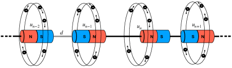
The particular phononic lattice under consideration is a system of repelling magnetic masses with grounding stiffness controlled by electrical coils driven applied voltage signals that are given by a time-periodic step function. The experimental setup is adapted form the platform developed in [15, 25]. The chain is composed of ring magnets (K&J Magnetic, Inc., P/N R848) lined with sleeve bearings (McMaster-Carr P/N 6377K2) comprising the uniform masses, arranged with alternating polarity on a smooth rod (McMaster-Carr P/N 8543K28). Electromagnetic coils (APW Company SKU: FC-6489) are fixed concentrically around the equilibrium positions of each of the innermost eight masses, such that they may exert a restoring force on each mass proportional to the current induced by applied voltage step-function (Aglient 33220A, Accel Instruments TS250-2). The velocity of each mass is measured using laser Doppler vibrometer (Polytec CLV-2534), repeating experiments to a construct full velocity field for the lattice. Figure 1 shows a schematic of the experimental setup.
The system is modeled as Fermi-Pasta-Ulam-Tsingou type lattice [15, 25]
| (1) |
where is the displacement of the th ring magnet from its equilibrium position, where the equilibrium distance between adjacent magnets is m. The indices run from and we consider fixed boundary conditions . All ring magnets have uniform mass kg. Dissipative forces are modeled with a phenomenological viscous damping term , where the damping coefficient Ns/m is determined empirically by matching the simulated and experimental spatial decay of the velocity amplitude envelope of waves traveling through the lattice [25]. The coupling force term is defined using the repulsive magnetic force between neighboring masses. The experimentally measured force-distance relation between neighboring masses is fit with a dipole-dipole approximation, as in [15], which is given by , where is the center-to-center distance between masses with and . The current resulting from a periodic step function voltage applied to the electromagnetic coils induces a magnetic field that provides a grounding stiffness modulation of the form
| (2) |
The step values and duty-cycle () are parameters. Unless otherwise stated, we use , N/m and s. We will use the modulation frequency Hz as the main system parameter to be varied.
III Modulation Instability
To find breathers, we first need to determine the wavenumber bandgap. This is achieved by computing the stability of plane waves (i.e., the modulation stability) of the linearized model
| (3) |
where . For time-independent stiffness the undamped () linear equation has the dispersion relationship such that the linear spectrum extends from and all plane waves are stable.
(a)
 (b)
(b)
In the case of time-dependent stiffness a gap in the wavenumber axis is possible. For general time-periodic stiffness with period , a wavenumber bandgap will open where the dispersion curve intersects itself when translated by an integer multiple of half the modulation frequency [36]. The advantage of considering to be a periodic step function is that the modified dispersion relation can be computed exactly. Making the ansatz , one finds upon substitution into Eq. (3) and enforcing Dirichlet boundary conditions that the eigenfunctions are where the wavenumber is with . In the infinite lattice, . The associated eigenvalues are . The temporal part satisfies
| (4) |
We can obtain an exact solution of this equation (and dispersion relation and stability condition), by adapting a procedure carried out in the context of an undamped Kronig-Penney photonic lattice [37, 38]. The general solution of Eq. (4) will be a superposition of functions of the form where has period and is the Floquet exponent where . The Floquet multiplier is . The waveform associated to the wavenumber will be stable if , or equivalently, if the Floquet multiplier has modulus less than unity, . Substitution of into equation (4) and demanding that and are continuous at and leads to the following equations (detailed in the Supplemental Material)
| (5) | |||||
| (6) |
where depends on the wavenumber and system parameters, but not the Floquet exponent :
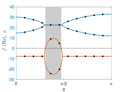
where . These equations allow for the exact computation of the Floquet exponents . An example plot is shown in Fig. 2(a). If then and . In this case the underlying solution is stable. If then , implying that the imaginary part of the Floquet exponent is an integer multiple of half the modulation frequency. In this case, the real part of the Floquet exponent is which implies the following condition for stability,
| (7) |
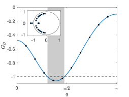
Note that this expression is exact and gives an efficient way to check for stability via direct substitution of the system parameters into and simply checking the inequality. A plot of is shown in Fig. 2(b). The linear stability predictions agree well with experimental observations (examples given in the Supplemental Material). The set of wavenumbers where make up the so-called wavenumber bandgap. The edges can be found by solving . See the gray regions of Fig. 2 for example wavenumber bandgaps.
(a)
 (b)
(b)
 (c)
(c)
IV Wavenumber Bandgap Breathers
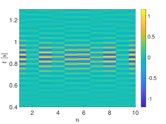
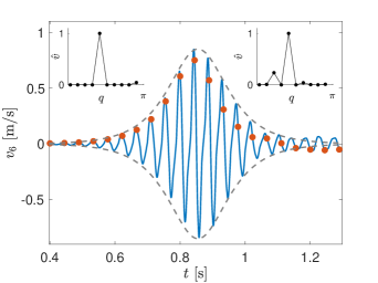
To draw analogy to the classic breathers of space-periodic systems, we first consider Eq. (1) without damping . To generate a wavenumber bandgap breather, Eq. (1) is initialized with an unstable plane wave, e.g., , where where is the wavenumber bandgap, , and the initial velocity is determined via Eq. (4). An example is shown in Fig. 3 with Hz, and wavenumber , which falls into the gap . The Floquet exponent associated to this wavenumber is . The corresponding Floquet multiplier is shown in the inset of Fig. 2(b) (the smaller of the two multipliers lying outside the unit circle).
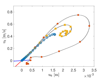
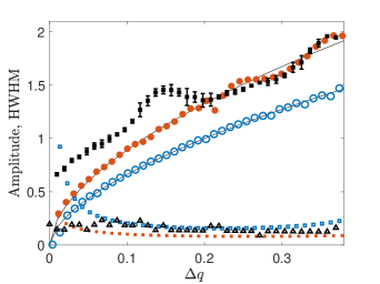
The solution initially grows exponentially with growth rate given by , due to the modulation instability, but reaches a turning point and then decays with the rate . This happens uniformly within the lattice, as shown by the intensity plot in Fig. 3(a). Figure 3(b) shows the time series of the velocity of the 6th node, i.e., (solid blue curve). Both panels (a) and (b) demonstrate that the dynamics are localized in time. Spatial periodicity of the solution is imposed by construction due to the finite length of the lattice with zero boundary conditions. The role of space and time have been switched when compared to the classic breathers of space-periodic systems. Thus, the solution shown in Fig. 3 is the so-called called wavenumber bandgap breather. Motivated by the fact that the envelope of a breather of a space-periodic FPUT lattice is described by a soliton of the Nonlinear Schrödinger (NLS) equation (in the limit of the temporal frequency approaching the band edge from within the spectral gap), we fit the velocity profile with a function of the form where are fitting parameters and is the real part of the Floquet exponent. See the gray dashed line of Fig. 3(b). The good agreement between the velocity profile and the fit envelope function confirms that the growth/decay rate is indeed given by the real part of the associated Floquet exponent, in this case . To better understand the mechanism behind the formation of the wavenumber bandgap breather, we construct a Poincaré map of the dynamics by sampling the solution with the frequency associated with the breather, namely . This corresponds to twice the period of the modulation. Thus, the map will be of the form , where is an integer, is the period of , and is vector valued solution of Eq. (1) with initial value . As in the simulation shown in Fig. 3(b), the initial value of the map is given by an unstable plane wave (e.g., with wavenumber ). The red dots of Fig. 3(b) show values of the map that correspond to . The red dots of Fig. 3(c) show values of in the phase plane. The eigenvector corresponding to the unstable (stable) Floquet exponent () is shown in red (blue). The gray line of Fig. 3(c) is obtained by repeatedly generating the map in the plane for various (small) multiples of the initial value . The origin is a saddle type fixed point, and the trajectory forms a near homoclinic orbit, made possible by the nonlinearity of the system. The orbit is not exactly homoclinic, since it does not approach the origin via the stable eigenvector as . Indeed, as can also be inferred from Fig. 3(b), the solution does not decay to zero, but rather it experiences small oscillations. This is due to the existence of other modes in the system (e.g., ones with associated multipliers lying on the unit circle), which are excited during the dynamic evolution. The insets of Fig. 3(b) show a normalized spatial Fourier transform of the signal before (the left inset) and after (the right inset) the maximum velocity is attained. In particular, the quantity is shown against the wavenumber, where where s and s are the times used to compute the transform before and after the turning point, respectively. Before the turning point the only prominent wavenumber is the one associated to the initial value (in this case ). After the turning point, there is an additional mode excited that lies outside the wavenumber bandgap (in this case ). It is this mode that is primarily responsible for the non-zero oscillations at the tail of the breather. If one imposes the additional criterion that a breather must have tails decaying to zero, then strictly speaking, the structure found here would be a generalized breather, since the orbit is not exactly homoclinic. Classic breathers with tails that do not decay to zero are common in non-integrable systems, and have sometimes been referred to as generalized breathers [39]. Over longer time windows, the amplitude of the signal can grow again (leading to a repeated appearance of breathers), but eventually the structure typically breaks down, leading to chaotic type dynamics for long-time simulations. Similar observations have been made for k-gap solitons in photonic systems [29]. The existence of perfectly homoclinic solutions in this system is an important question, but it lies beyond the scope of the present article. Inspection of the long time dynamics, as well as breathers for other parameter values, are provided in the Supplemental Material. We now generate a family of wavenumber bandgap breathers parameterized by the distance the underlying wavenumber is from the band edge . This is a natural parameter to consider, as the distance to the bandedge determines breather width and amplitude in space-periodic systems [1]. Keeping all parameters fixed, but gradually varying the modulation frequency has the effect of shifting the bandgap in the wavenumber axis. Thus, we fix the wavenumber ( in this case), whose distance to the right edge will increase as the modulation frequency is increased. For the breather shown in Fig. 3 the distance to the edge is . The red dots of Fig. 4(a) show the amplitude of the breather vs. . The amplitude is computed as the maximum velocity of the 6th node, i.e., . For the breathers do not form a coherent localization, like in Fig. 3. Similar simulations with wavenumber near the left edge of the bandgap () did not lead to the robust formation of breathers. The amplitude data is fit with a function of the form , with the best fit values being and (the solid line in Fig. 4(a)). This is consistent with the trend found for classic breathers in space-periodic systems where it is well known that the breather amplitude grows like , where is the difference between the breather frequency and the edge of the frequency spectrum [1].
(a)
 (b)
(b)
 (c)
(c)
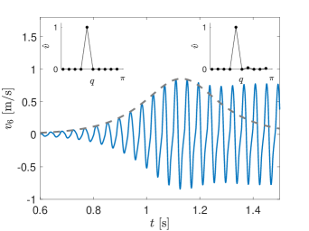
Now that we have established the existence of wavenumber bandgap breathers in Eq. (1), we now consider the role of damping, which will bring us closer to the experimentally relevant situation. Breathers in experiments will always be a dissipative analog of breathers in lossless models. Thus, we modify our definition of a breather to account for dissipative effects. To motivate our modified definition, we repeat the simulations shown in Fig. 3 but with a nonzero damping parameter. The yellow square (blue circle) markers of Fig. 3(c) show the orbit with a damping parameter of () Ns/m. The orbit starts close to being homoclinic, but the dynamics are attracted to a stable fixed point (i.e., a time-periodic orbit of the original system with period ). Note that the time-dependent stiffness term in the model (with the coefficient) acts as an effective gain term to balance loss. The orbit in the damped system experiences an initial exponential growth and a turning point, like the lossless breather, but rather than approaching near zero amplitude, the dynamics tend to a stable fixed point. Thus, the left tail of the “damped breather” (in the time domain) is much like a lossless breather, whose amplitude is slightly lower due to the presence of damping. The right tail of the “damped breather” approaches a periodic oscillation, whose amplitude is not necessarily small relative to the amplitude of the breather. See Fig. 4(b) for an example time series with Ns/m. An alternative classification for the structure found in the damped system would be a wavenumber bandgap “front”, since the solution is heteroclinic, as it connects the unstable zero fixed point to a non-zero stable fixed point. Important for the present study, however, is that the transition between the zero and nonzero state is approximately described by the lossless breather (i.e., the near homoclinic orbit). We measure the amplitude of the structure in the same way we measured the breather amplitude in the lossless system, i.e., . We repeat this for various modulation frequencies (and hence values) for the damping value Ns/, which is shown as the blue circle markers in Fig. 4(a). The qualitative amplitude trend is similar to the lossless case, but the amplitude is decreased. The amplitude data in the damped case is also fit with a function of the form , with the best fit values being and .
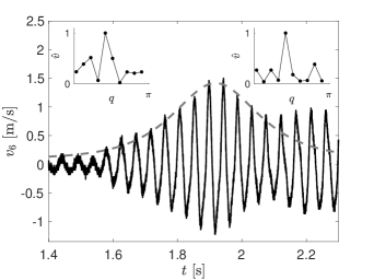
We now turn to the experimental construction of wavenumber bandgap breathers (using the dissipative definition of a breather defined above). To excite a plane wave with a particular wavenumber (in this case ) the unmodulated system is driven with the frequency . Once the desired plane wave is excited, the initial driving is turned off and the modulation is turned on simultaneously. Like in the damped simulation, the amplitude will initially grow, reach a turning point, decay, but eventually approach a periodic orbit (or exhibit chaotic behavior). An example experimental time series is shown in Fig. 4(c). Notice the qualitative agreement to the theoretical prediction shown in Fig. 4(b). Since the band edge can only be computed in the infinite lattice, we use the relation , where is found analytically. In general, there will be a mistuning between the experimental and model dynamics for a fixed modulation frequency. We account for this mistuning by measuring the modulation frequency the mode becomes unstable in the model and experiment. The difference between the experimental and theoretical critical modulation frequencies, , is then added to the experimental modulation frequencies when calculating the distance to the band edge, namely . Thus, corresponds to the frequency at which becomes unstable for both experiment and model. The mode associated to is considered unstable when its corresponding amplitude in Fourier space exceeds a noise threshold (details given in the Supplemental Material). With these definitions in place, we now measure the amplitude of the breather as a function of , see the markers with error bars in Fig. 4(a). The qualitative amplitude trend agrees with the theoretical prediction. Although the time series between the theoretical prediction for Ns/m and the experiment agree qualitatively (compare panels (b) and (c) of Fig. 4) the model underestimates the amplitude. This can be partially explained by the fact that other modes (including unstable ones) in the experiment besides are excited. Inspection of the spatial Fourier transform of the experiment shows there are always traces of additional modes, even before the turning point of the structure. The insets of Fig. 4(c) show the spatial Fourier transform before ( s) and after ( s) the turning point (more details of the Fourier analysis of the experiment is given in the Supplemental Material).
Finally, we measure the width of the structures using the half-width at half maximum (HWHM) metric. The HWHM is given by , where is the time the maximum is attained and is the time where the trajectory first attains half the maximum value. The experimentally measured values are shown as the black triangles in Fig. 4(a). The width of the structure can be predicted theoretically using the real part of the Floquet exponent. In particular, assuming the envelope of the breather follows the form (which we demonstrated previously was a reasonable assumption), we can compute the HWHM as . The prediction in the lossless () and damped ( Ns/m) cases are shown as red solid squares and open blue squares, respectively, in Fig. 4(a). For sufficiently large values of , there is good agreement between theory and experiment, and both show the structure becomes more narrow as the wavenumber goes deeper into the gap. This is consistent with classic breathers in space-periodic systems.
V Conclusion
We explored a new class of solutions, phononic wavenumber bandgap breathers and their damped analogues, in a time-varying lattice. Several avenues of inquiry follow naturally from this study, including the possible existence of genuine q-gap breathers (i.e., with both tails decaying to zero), an analytical description of the breather profiles via a multiple-scale analysis, and the exploration of such structures in higher spatial dimensions.
Acknowledgement. This material is based upon work supported by the US National Science Foundation under Grant Nos. EFRI-1741565 (C.D.) and DMS-2107945 (C.C. and E.W.). The authors are grateful for discussions with P.G. Kevrekidis.
References
- [1] S. Flach and A. Gorbach. Discrete breathers: advances in theory and applications. Phys. Rep., 467:1, 2008.
- [2] P. G. Kevrekidis. Non-linear waves in lattices: Past, present, future. IMA J. Appl. Math., 76:389–423, 2011.
- [3] S V Dmitriev, E A Korznikova, Yu A Baimova, and M G Velarde. Discrete breathers in crystals. Physics-Uspekhi, 59(5):446–461, 2016.
- [4] G. Huang and B. Hu. Asymmetric gap soliton modes in diatomic lattices with cubic and quartic nonlinearity. Phys. Rev. B, 57:5746, 1998.
- [5] S. Flach, M. V. Ivanchenko, and O. I. Kanakov. -Breathers and the Fermi-Pasta-Ulam Problem. Phys. Rev. Lett., 95:064102, 2005.
- [6] Marin Soljačić, Mihai Ibanescu, Steven G. Johnson, Yoel Fink, and J. D. Joannopoulos. Optimal bistable switching in nonlinear photonic crystals. Physical Review E, 66(5):055601, 2002.
- [7] F. Y. Wang, G. X. Li, H. L. Tam, K. W. Cheah, and S. N. Zhu. Optical bistability and multistability in one-dimensional periodic metal-dielectric photonic crystal. Applied Physics Letters, 92(21):211109, 2008.
- [8] Chao-Peng Wen, Wei Liu, and Jian-Wei Wu. Tunable terahertz optical bistability and multistability in photonic metamaterial multilayers containing nonlinear dielectric slab and graphene sheet. Applied Physics A, 126(6):426, 2020.
- [9] Sebabrata Mukherjee and Mikael C. Rechtsman. Observation of unidirectional solitonlike edge states in nonlinear floquet topological insulators. Phys. Rev. X, 11:041057, 2021.
- [10] David A. Powell, Ilya V. Shadrivov, and Yuri S. Kivshar. Multistability in nonlinear left-handed transmission lines. Applied Physics Letters, 92(26):264104, 2008.
- [11] Alexander B. Kozyrev, Hongjoon Kim, and Daniel W. van der Weide. Parametric amplification in left-handed transmission line media. Applied Physics Letters, 88(26):264101, 2006.
- [12] David A. Powell, Ilya V. Shadrivov, and Yuri S. Kivshar. Asymmetric parametric amplification in nonlinear left-handed transmission lines. Applied Physics Letters, 94(8):084105, 2009.
- [13] E.S. Cassedy. Dispersion relations in time-space periodic media part II—Unstable interactions. Proceedings of the IEEE, 55(7):1154–1168, 1967.
- [14] J. R. Reyes-Ayona and P. Halevi. Observation of genuine wave vector ( or ) gap in a dynamic transmission line and temporal photonic crystals. Applied Physics Letters, 107(7):074101, 2015.
- [15] Yifan Wang, Behrooz Yousefzadeh, Hui Chen, Hussein Nassar, Guoliang Huang, and Chiara Daraio. Observation of nonreciprocal wave propagation in a dynamic phononic lattice. Physical Review Letters, 121(19):194301, 2018.
- [16] E. Galiffi, P.A. Huidobro, and J.B. Pendry. Broadband Nonreciprocal Amplification in Luminal Metamaterials. Physical Review Letters, 123(20):206101, 2019.
- [17] Giuseppe Trainiti, Yiwei Xia, Jacopo Marconi, Gabriele Cazzulani, Alper Erturk, and Massimo Ruzzene. Time-Periodic Stiffness Modulation in Elastic Metamaterials for Selective Wave Filtering: Theory and Experiment. Physical Review Letters, 122(12):124301, 2019.
- [18] Seojoo Lee, Jagang Park, Hyukjoon Cho, Yifan Wang, Brian Kim, Chiara Daraio, and Bumki Min. Parametric oscillation of electromagnetic waves in momentum band gaps of a spatiotemporal crystal. Photonics Research, 9(2):142, 2021.
- [19] G. Trainiti and M. Ruzzene. Non-reciprocal elastic wave propagation in spatiotemporal periodic structures. New Journal of Physics, 18(8):083047, 2016.
- [20] Benjamin M. Goldsberry, Samuel P. Wallen, and Michael R. Haberman. Non-reciprocal wave propagation in mechanically-modulated continuous elastic metamaterials. The Journal of the Acoustical Society of America, 146(1):782–788, 2019.
- [21] Yangyang Chen, Xiaopeng Li, Hussein Nassar, Andrew N. Norris, Chiara Daraio, and Guoliang Huang. Nonreciprocal Wave Propagation in a Continuum-Based Metamaterial with Space-Time Modulated Resonators. Physical Review Applied, 11(6):064052, 2019.
- [22] Xiaohui Zhu, Junfei Li, Chen Shen, Xiuyuan Peng, Ailing Song, Longqiu Li, and Steven A. Cummer. Non-reciprocal acoustic transmission via space-time modulated membranes. Applied Physics Letters, 116(3):034101, 2020.
- [23] J. Marconi, E. Riva, M. Di Ronco, G. Cazzulani, F. Braghin, and M. Ruzzene. Experimental Observation of Nonreciprocal Band Gaps in a Space-Time-Modulated Beam Using a Shunted Piezoelectric Array. Physical Review Applied, 13(3):031001, 2020.
- [24] Hussein Nassar, Behrooz Yousefzadeh, Romain Fleury, Massimo Ruzzene, Andrea Alù, Chiara Daraio, Andrew N. Norris, Guoliang Huang, and Michael R. Haberman. Nonreciprocity in acoustic and elastic materials. Nature Reviews Materials, 5:667–685, 2020.
- [25] B. L. Kim, C. Chong, S. Hajarolasvadi, Y. Wang, and C. Daraio. Dynamics of time-modulated, nonlinear phononic lattices. Phys. Rev. E, 107:034211, 2023.
- [26] Lei Liu, Wen-Rong Sun, Boris A. Malomed, and P. G. Kevrekidis. Time-localized dark modes generated by zero-wave-number-gain modulational instability. Phys. Rev. A, 108:033504, 2023.
- [27] Nail Akhmediev, Adrian Ankiewicz, and J. M. Soto-Crespo. Rogue waves and rational solutions of the nonlinear Schrödinger equation. Phys. Rev. E, 80:026601, 2009.
- [28] Adrian Ankiewicz, Nail Akhmediev, and J. M. Soto-Crespo. Discrete rogue waves of the Ablowitz-Ladik and Hirota equations. Phys. Rev. E, 82:026602, 2010.
- [29] Yiming Pan, Moshe-Ishay Cohen, and Mordechai Segev. Superluminal -gap solitons in nonlinear photonic time crystals. Phys. Rev. Lett., 130:233801, 2023.
- [30] Adarsh Ganesan, Cuong Do, and Ashwin Seshia. Phononic frequency comb via intrinsic three-wave mixing. Phys. Rev. Lett., 118:033903, 2017.
- [31] L. S. Cao, D. X. Qi, R. W. Peng, Mu Wang, and P. Schmelcher. Phononic frequency combs through nonlinear resonances. Phys. Rev. Lett., 112:075505, 2014.
- [32] Mengjie Yu, Jae K. Jang, Yoshitomo Okawachi, Austin G. Griffith, Kevin Luke, Steven A. Miller, Xingchen Ji, Michal Lipson, and Alexander L. Gaeta. Breather soliton dynamics in microresonators. Nature Communication, 8:14569, 2017.
- [33] Geon Lee, Dongwoo Lee, Jeonghoon Park, Yeongtae Jang, Miso Kim, and Junsuk Rho. Piezoelectric energy harvesting using mechanical metamaterials and phononic crystals. Commun Phys, 5:94, 2022.
- [34] Mohsen Safaei, Henry A Sodano, and Steven R Anton. A review of energy harvesting using piezoelectric materials: state-of-the-art a decade later (2008–2018). Smart Materials and Structures, 28(11):113001, 2019.
- [35] William Hartmann. Acoustic Signal Processing, pages 503–530. Springer New York, New York, NY, 2007.
- [36] H. Nassar, X. C. Xu, A. N. Norris, and G. L. Huang. Modulated phononic crystals: Non-reciprocal wave propagation and Willis materials. Journal of the Mechanics and Physics of Solids, 101:10–29, 2017.
- [37] Martin Centurion, Mason A. Porter, Ye Pu, P. G. Kevrekidis, D. J. Frantzeskakis, and Demetri Psaltis. Modulational instability in nonlinearity-managed optical media. Phys. Rev. A, 75:063804, 2007.
- [38] Z Rapti, G Theocharis, P G Kevrekidis, D J Frantzeskakis, and B A Malomed. Modulational instability in bose–einstein condensates under feshbach resonance management. Physica Scripta, 2004(T107):27, 2004.
- [39] Mark D. Groves and Guido Schneider. Modulating pulse solutions for quasilinear wave equations. Journal of Differential Equations, 219(1):221–258, 2005.