Quantum Shadow Gradient Descent for Quantum Learning

Abstract

Gradient-based techniques are commonly used for training in variational quantum algorithms (VQAs) for optimization and learning using quantum computers. The computation of the gradient in quantum settings is challenging due to the stochastic nature of quantum measurements, associated state collapse, the no-cloning principle, and measurement incompatibility. Prior approaches, such as zeroth-order and first-order methods, address only some of these challenges and suffer from slow convergence rates and high copy complexity. This paper proposes a new procedure called quantum shadow gradient descent (QSGD) that addresses these key challenges. Our method has the benefits of a one-shot approach, in not requiring any sample duplication while having a convergence rate comparable to the ideal update rule using exact gradient computation. We propose a new technique for generating quantum shadow samples (QSS), which generates quantum shadows as opposed to classical shadows used in existing works. With classical shadows, the computations are typically performed on classical computers and, hence, are prohibitive since the dimension grows exponentially. Our approach resolves this issue by measurements of quantum shadows. As the second main contribution, we study more general non-product ansatz of the form $\exp\{i\sum_{j}\theta_{j}A_{j}\}$ that model variational Hamiltonians. We prove that the gradient can be written in terms of the gradient of single-parameter ansatzes that can be easily measured. Our proof is based on the Suzuki-Trotter approximation; however, our expressions are exact, unlike prior efforts that approximate non-product operators. As a result, existing gradient measurement techniques can be applied to more general VQAs followed by correction terms without any approximation penalty. We provide theoretical proofs, convergence analysis and verify our results through numerical experiments.

1 Introduction

Learning and optimization represent important applications of quantum computers in the context of classical and quantum data. VQA are commonly applied to these problems for training/ tuning quantum models. They rely on a parameterized model of a quantum computer (a.k.a. ansatz) that is tuned via a hybrid quantum-classical loop. The learned model is a quantum operator, whose parameters are optimized using a classical procedure, on quantum training samples (Farhi and Neven 2018; Heidari, Grama, and Szpankowski 2022; Schuld et al. 2020). VQAs operate either directly on quantum training data (Carrasquilla and Melko 2017; Carleo and Troyer 2017), or by mapping classical data into input quantum states (Lloyd, Mohseni, and Rebentrost 2014). They also have been studied in the specific context of quantum neural networks  (Farhi and Neven 2018).

Approaches based on stochastic gradient descent (SGD) are commonly used for minimizing loss (Mitarai et al. 2018; Schuld et al. 2020; Harrow and Napp 2021) in VQAs. These methods rely on an approximation of the gradient of the training loss with respect to the parameters of the ansatz. Exact computation of the gradient is impossible since it is a function of the loss, which itself is an expectation value. This expectation value depends on the input quantum state, whose characterization is typically unknown. Hence, the computation of this expectation requires an infinite number of measurements. Consequently, only approximations of the gradient can be used in quantum settings. There are several proposed solutions to this problem. In Zeroth-order or finite-differencing methods, the gradient is approximated by directly evaluating the empirical loss under slightly shifted parameters (Kandala et al. 2017; Harrow and Napp 2021; Farhi, Goldstone, and Gutmann 2014). First-order methods (a.k.a. analytic gradient measurements) are a recent alternative based on direct measurement of the gradient, without necessarily evaluating the loss (Mitarai et al. 2018; Gilyén, Arunachalam, and Wiebe 2019; Schuld et al. 2018). They rely on approximating the expected value of the observables, directly measuring the derivatives of the loss. These methods can lead to faster convergence rates compared to the zeroth-order approaches (Harrow and Napp 2021). Both of these methods typically require large numbers of measurements to estimate expectation values accurately, leading to high repeat complexity. Specifically, training a VQA with $c$ parameters using current methods requires $\order{\frac{1}{\epsilon^{2}}c\log c}$ rounds of circuit utilization, where $\epsilon\ll 1$ is the estimation error. A recent alternative, called parameter shift, proposes “stochastic estimation” of the gradient using a fixed number of measurements in each iteration (Harrow and Napp 2021; Sweke et al. 2020). Although this approach reduces the overhead of previous methods, it still requires a large number of training samples for accurate estimation.

SGD optimizations rely on estimators of the gradient (a.k.a. sub-gradients) (Shalev-Shwartz and Ben-David 2014) and have provable convergence guarantees when the estimator is unbiased and the loss satisfies certain constraints. At every step, the derivative of the loss function w.r.t. each ansatz parameter is measured by a specific derivative observable. Such observables are not necessarily compatible with each other (i.e., measurement by one observable may result in a state collapse and change w.r.t. others), and hence, cannot be measured simultaneously (Holevo 2012). As a result, fresh samples are needed for each derivative observable. This leads to a circuit repeat (and copy complexity) that scales linearly with the number of the ansatz’s parameters $c$. More importantly, because of the no-cloning postulate, exact copies of the samples are not feasible in many problems in optimization and learning. Recently, a new alternative called RQSGD was proposed, which addresses these issues  (Heidari, Grama, and Szpankowski 2022). The main idea is to randomly select one parameter and measure the corresponding derivative using a single measurement (i.e., using a single training data sample). The estimated gradient is a vector that is zero everywhere except at the selected component. Therefore, this method has a constant per-iteration overhead as it uses the circuit only once per iteration. Moreover, sample duplication is no longer needed. However, due to the serialization of updates, this approach suffers from slow convergence, particularly for ansatz with large parameter sets.

In conclusion, each of the aforementioned methods has significant drawbacks that we address in our work — parameter-shift, zeroth or first-order methods have high circuit overhead and need several exact sample copies, and one-shot methods suffer from slow convergence due to measurement-compatibility constraints. Moreover, except zeroth-order methods, other approaches do not apply to general ansatzes, as they assume only products of forms $e^{i\theta_{1}A_{1}}e^{i\theta_{2}A_{2}}\cdots e^{i\theta_{m}A_{m}},$ where $\theta_{j}$’s are the parameters. Our work resolves all of these issues through a novel method called “shadow quantum gradient descent (QGD)”. Our approach has a constant copy complexity and achieves a convergence rate similar to the ideal method based on the exact gradient computation. Furthermore, through a novel transformation, our method is applicable to general ansatz that can be expressed in both product- and non-product forms.

Summary of the main contributions

The main contributions of this paper are two-fold: (i) a new gradient-based method called “quantum shadow gradient descent” (QSGD) for training quantum models (Section 3). This method has the benefits of a one-shot approach (such as RQSGD) in not requiring any sample duplication while having a faster, near-optimal convergence rate; and (ii) using Trotter-Suzuki decomposition (Suzuki 1976) to design a novel approach to measure the gradient of the loss for general non-product ansatz (Section 3). Our approach for QSGD builds on a new technique for generating quantum shadow samples (QSS); see Section 3. Shadow generation from quantum states has been studied before in the context of state tomography (Aaronson 2018; Huang, Kueng, and Preskill 2020). In our work, we generalize this concept to the broader context of optimization and learning and propose a novel, fully quantum variation of the concept. Prior approaches based on shadow tomography rely on classical shadows with computations done on classical computers and, hence, are prohibitive in terms of their dimensionality. Our approach resolves this issue by estimating states via measurements of quantum shadows on a QC. We show that QSS has a scalable implementation with a $\order{\log\dim}$ gate complexity. For the second main contribution, we prove that the gradient of a non-product unitary can be written in terms of the gradient of single-parameter ansatzes that can be easily measured (Theorem 1). Unlike prior efforts that approximate non-product operators, our expressions are exact. As a result, one can apply existing gradient measurement techniques, followed by correction terms, to a more general class of non-product ansatzes, such as QNNs, without any approximation penalty. Such non-product ansatzes have been studied in the literature for quantum simulation and optimization with parameterized Hamiltonian (Kairys and Humble 2021; Miessen, Ollitrault, and Tavernelli 2021). To the best of our knowledge, our method is the first to achieve near-ideal convergence with one copy complexity and be applicable to general ansatzes. We provide comprehensive theoretical analysis for all claims and verify our results experimentally through numerical experiments.

Related results

There has been significant recent interest in the development of VQAs and QNNs – we highlight closely related results here. VQAs, in general, have been studied for a variety of problems involving quantum or classical data (Cerezo et al. 2020; Guerreschi and Smelyanskiy 2017). Learning from quantum data has been studied extensively in recent literature in the context of diverse applications, including phase-of-matter detection (Carrasquilla and Melko 2017; Broecker et al. 2017), ground-state search (Carleo and Troyer 2017; Broughton et al. 2020; Biamonte et al. 2017), entanglement detection (Ma and Yung 2018; Massoli et al. 2021; Lu et al. 2018; Hiesmayr 2021; Chen et al. 2021; Deng, Li, and Sarma 2017), and related problems in theoretical chemistry (Kassal et al. 2011; McArdle et al. 2020; Hempel et al. 2018; Cao et al. 2019; Bauer et al. 2020). VQAs are also applicable to classical data by mapping them to input quantum states (Giovannetti, Lloyd, and Maccone 2008; Park, Petruccione, and Rhee 2019; Rebentrost, Mohseni, and Lloyd 2014; Lloyd, Mohseni, and Rebentrost 2013, 2014). QNNs have received significant research attention since the early work (Toth et al. 1996; Lewenstein 1994) to more recent developments over the past two decades (Schuld, Sinayskiy, and Petruccione 2014; Mitarai et al. 2018; Farhi and Neven 2018; Torrontegui and Garcia-Ripoll 2018; Schuld et al. 2020; Beer et al. 2020). Massoli et al. provide an excellent survey of these efforts (Massoli et al. 2021). VQAs have also been applied to the specific context of QNNs  (Mitarai et al. 2018; Farhi and Neven 2018; Schuld et al. 2020; Beer et al. 2020; Heidari, Grama, and Szpankowski 2022; Cerezo et al. 2020; Guerreschi and Smelyanskiy 2017).

2 Preliminaries and Model

Notation: For any $d\in\mathbb{N}$, we denote the set $\left\{1,2,...,d\right\}$ by $[d]$, and represent by $H_{d}$ the Hilbert space of $d$-qubits of dimension $2^{d}$. The identity operator on $H_{d}$ is denoted by $I_{d}$. A quantum state is defined as a density operator; that is, a Hermitian, unit-trace, and non-negative linear operator. A quantum measurement $\mathcal{M}$ is a positive operator-valued measure (POVM) represented by a set of operators $\mathcal{M}:=\{M_{v},v\in\mathcal{V}\}$, where $\mathcal{V}$ is the set of possible outcomes, $M_{v}\geq 0$ for any $v\in\mathcal{V}$, and $\sum_{v\in\mathcal{V}}M_{v}=I_{d}.$ The single-qubit Pauli operators, along with the identity operator are denoted by $\sigma^{0}:=I,\sigma^{1}:=X,\sigma^{2}:=Y,$ and $\sigma^{3}:=Z$. Furthermore, $d$-fold tensor products of these operators are denoted by $\sigma^{\mathbf{s}}:=\operatorname*{\otimes}_{j}\sigma^{s_{j}}$, where $\mathbf{s}\in\left\{0,1,2,3\right\}^{d}$.

Quantum learning model

The ansatz, a parameterized quantum operation, is an essential component in the design of VQAs. An ansatz is modeled as a (unitary) operation $U(\overrightarrow{a})$, with $\overrightarrow{a}$ being the vector of model parameters. This model also generalizes the notion of QNNs. The objective of a learner/ trainer is to minimize the loss by tuning the parameters of the ansatz. The loss function is defined in a problem-specific manner. Our model of quantum learning inputs a number of quantum states (training samples) with associated classical labels (Heidari, Padakandla, and Szpankowski 2021). Note that classical descriptions of these input quantum states are unknown. Labeled quantum samples $(\ket{\phi_{i}},y_{i}),i\in[n]$ are randomly generated independent and identically distributed (i.i.d.) according to an unknown but fixed probability distribution $D$. Labels $y_{i}$ are drawn from a set $\mathcal{Y}$, and the states $\ket{\phi_{i}}$ exist in a (finite-dimensional) Hilbert space. The objective is to accurately predict the label of unseen samples by applying an ansatz $U(\overrightarrow{a})$, followed by a fixed quantum measurement $\mathcal{M}:=\left\{M_{\hat{y}}:\hat{y}\in\mathcal{Y}\right\}$. Let $\hat{y}\in\mathcal{Y}$ be the predicted label. From Born’s rule, $\hat{y}$ is generated randomly with probability:

$$\mathbb{P}\Big{\{}\hat{Y}=\hat{y}|\ket{\phi},\overrightarrow{a}\Big{\}}=\expectationvalue{U^{\dagger}(\overrightarrow{a})M_{\hat{y}}U(\overrightarrow{a})}{\phi}.$$

The incurred prediction loss is determined via a loss function $l:\mathcal{Y}\times\mathcal{Y}\rightarrow[0,\infty)$. Unlike classical learning, the prediction loss is random even for a fixed input. Conditioned on a fixed sample $(\ket{\phi},y)$, the sample’s expected loss taken w.r.t. $\hat{Y}$ is given by:

$$\mathcal{L}( \overrightarrow{a},\ket{\phi},y)=\sum_{\hat{y}\in\mathcal{Y}}\ell(y,\hat{y})\expectationvalue{U^{\dagger}(\overrightarrow{a})M_{\hat{y}}U(\overrightarrow{a})}{\phi}.$$

Taking expectation over the sample’s distribution $D$ gives the generalization (expected) loss as a function of $\overrightarrow{a}$:

$$\mathcal{L}(\overrightarrow{a}) =\mathbb{E}_{D}[\mathcal{L}(\overrightarrow{a},\ket{\phi},Y)].$$ (1)

The objective is to minimize expected loss by optimizing parameters. While it is desirable to minimize expected loss, this goal is not feasible since the underlying distribution $D$ is unknown. Hence, this problem is more challenging than the corresponding standard optimization in VQA settings. While $D$ and the quantum sample statesare unknown, we have access only to a set of quantum samples $(\ket{\phi}_{i},y_{i}),i\in[n]$ as the training set. Hence, one aims to tune the ansatz by minimizing the average per-sample expected loss: $\frac{1}{n}\sum_{t=1}^{n}\mathcal{L}(\overrightarrow{a},\ket{\phi_{t}},y_{t}).$

Gradient-Based Optimization

We focus on gradient-based approaches in this paper. While this appears similar to the classical learning problem, quantum mechanical postulates pose significant challenges that we address in this paper. Ideally, if the per-sample expected loss $\mathcal{L}(\overrightarrow{a},\ket{\phi_{t}},y_{t})$ were known, one would apply a standard gradient descent method via an update rule of the form:

$$\overrightarrow{a}^{(t+1)}=\overrightarrow{a}^{(t)}-\eta_{t}\nabla\mathcal{L}(\overrightarrow{a},\ket{\phi_{t}},y_{t}).$$ (2)

This update rule is infeasible in practice, as the exact value of the gradient is unknown. This is because $\mathcal{L}(\overrightarrow{a},\rho_{t},y_{t})$ is an expectation value, and also, the superposition coefficients of $\ket{\phi_{t}}$ are unknown. Computing those coefficients requires infinitely many measurements, which is infeasible; hence, one can only estimate/ approximate the gradient. The parameter optimization procedure must be consistent with quantum mechanical postulates such as no-cloning, state collapse, and measurement incompatibility (Holevo 2012).

No-Cloning:

The no-cloning postulate implies that unknown quantum samples cannot be replicated, thus prohibiting the use of several existing results (Farhi and Neven 2018; Mitarai et al. 2018; Sweke et al. 2020) in quantum learning applications, as they rely on repeated measurements on exact copies of the samples. Recent approaches (Heidari, Grama, and Szpankowski 2022) address these issues by introducing a one-shot training solution.

Measurement incompatibility:

Measurement incompatibility refers to the fact that certain properties of a quantum system cannot be simultaneously measured with arbitrary precision (Michael A. Nielsen 2010). Note that $\nabla\mathcal{L}$ corresponds to a vector of the derivatives of $\mathcal{L}$ with respect to different parameters. Each derivative $\frac{\partial\mathcal{L}}{\partial a}$ is obtained through an associated quantum measurement applied to the output state. Such quantum measurements are generally incompatible as the underlying operators do not commute with each other necessarily (Holevo 2012). As a result, the derivatives are not simultaneously measurable. Hence, even when approximating the gradient, one needs fresh batches of exact copies for each component of the gradient. Therefore, training methods based on gradient approximation (e.g., zeroth-order, and first-order methods) need $\order{c}$ exact copies for approximating the gradient with $c$ derivatives. Even when no-cloning is ignored, this dependency on $c$ is problematic, as $c$ can grow exponentially large.

3 Main Results

This section introduces our method, quantum stochastic gradient descent (QSGD), and provides theoretical underpinnings for its correctness and performance. First, in Section 3, we study the gradient of the loss for product and non-product ansatz. Specifically, we derive the Trotter-based expression for gradient of non-product ansatzes (Theorem 1). Next, in Section 3, we present our QSGD training method and describe our QSS method for quantum shadow generations. Lastly, in Section 3, we derive the convergence results (Theorem 3).

Gradient of the loss

The gradient $\nabla\mathcal{L}$ depends on the ansatz parametrization $U(\overrightarrow{a})$. We consider two generic formulations of the ansatz: product and non-product forms.

Product ansatz. This formulation, which is widely used in literature, is a unitary operator defined as

$$U(\overrightarrow{a}):=\prod_{r=1}^{k}\exp\{ia_{\mathbf{s}_{r}}\sigma^{\mathbf{s}_{r}}\},$$ (3)

where $k$ is the number of layers, $\mathbf{s}\in\left\{0,1,2,3\right\}^{d}$ and $\sigma^{\mathbf{s}_{r}}$ is the Pauli string associated with $\mathbf{s}_{r}$. For any $l\in[k]$, let $U_{\leq l}:=\prod_{r=1}^{l}e^{ia_{\mathbf{s}_{r}}\sigma^{\mathbf{s}_{r}}}$ denote the product till layer $l$. Similarly, let $U_{>l}:=\prod_{r>l}^{k}e^{ia_{\mathbf{s}_{r}}\sigma^{\mathbf{s}_{r}}}$ denote the products after $l$. The gradient of the loss is then computed as follows.

Lemma 1 ((Heidari, Grama, and Szpankowski 2022)).

Let ${\rho}_{l}^{out}=U_{\leq l}\rho U_{\leq l}^{\dagger}$ denote the density operator of the output state at layer $l$ when the input is $\rho$ with label $y$. Then, the derivative of the loss is given by:

$$\frac{\partial\mathcal{L}}{\partial a_{\mathbf{s}_{l}}}=\sum_{\hat{y}}i\ell(y,\hat{y})\tr{M_{\hat{y}}U_{>l}\big{[}\sigma^{\mathbf{s}_{l}},{\rho}_{l}^{out}\big{]}U^{\dagger}_{>l}},$$ (4)

where $[\cdot,\cdot]$ is the commutator operation.

For completeness, the proof is given in Appendix A.

Non-product ansatz.

We also consider a more general form of the ansatz. Note that any unitary operator is of the form $e^{iA}$ for some Hermitian operator $A$. Moreover, $A$ decomposes in terms of Pauli strings as $A=\sum_{\mathbf{s}}a_{\mathbf{s}}\sigma^{\mathbf{s}}$, where $\mathbf{s}\in\left\{0,1,2,3\right\}^{d}$ and $a_{\mathbf{s}}=2^{-d}\tr{A\sigma^{\mathbf{s}}}$. With these observations, we consider the following formulation of the ansatz:

$$U(\overrightarrow{a}):=\exp\{i\sum_{\mathbf{s}}a_{\mathbf{s}}\sigma^{\mathbf{s}}\Big{\}}.$$ (5)

Note that we can consider a multi-layered ansatz where each layer is of the above form. However, for simplicity, we consider only a single-layer ansatz. Due to the non-commutativity of the Pauli products, Lemma 1 does not apply. Hence, existing gradient estimation methods based on measurements, such as finite-difference and first-order, are not applicable to general ansatzes. We address this issue by proving the following result that decomposes the gradient into product forms.

We first need a few definitions. It is known that the product of the Pauli operators satisfies $\sigma_{j}\sigma_{k}=\delta_{jk}I+i\varepsilon_{jk\ell}\sigma_{\ell}$ for any $j\neq k\neq\ell\in\{1,2,3\}$, where $\delta_{jk}$ is the Kronecker delta and $\varepsilon_{jk\ell}$ is the Levi-Civita symbol. We extend this notation to include $\sigma_{0}=I$. For any $j,k,\ell\in\{0,1,2,3\}$, define $\kappa_{jk\ell}$ as follows: $\kappa_{jk\ell}$ equals $\delta_{k\ell}$ if $j=0$; else $\delta_{j\ell}$ if $k=0$; else $\delta_{0\ell}$ if $j=k$; and otherwise equals to $i\varepsilon_{jk\ell}$ when $j\neq k\neq 0$. With this definition, we can write $\sigma_{j}\sigma_{k}=\sum_{\ell=0}^{3}\kappa_{jk\ell}\sigma_{\ell}$. For vectors $\mathbf{r},\mathbf{s},\mathbf{t}\in\left\{0,1,2,3\right\}^{d}$ we extend this definition to $\kappa_{\mathbf{r}\mathbf{s}\mathbf{t}}=\prod_{j=1}^{d}\kappa_{r_{j}s_{j}t_{j}}$.

Theorem 1.

For a non-prodct ansatz $U(\overrightarrow{a})$ as in (5), let $\rho^{out}$ be the output state. For any $\mathbf{t}\in\left\{0,1,2,3\right\}^{d}$, define $\frac{\partial\tilde{\mathcal{L}}}{\partial a_{\mathbf{t}}}:=\sum_{\hat{y}}i\ell(y,\hat{y})\tr{M_{\hat{y}}\big{[}\sigma^{\mathbf{t}},{\rho}^{out}\big{]}}$, where $y$ is the true label. Then, the derivative of the loss for the non-product $U$ expands in terms of $\frac{\partial\tilde{\mathcal{L}}}{\partial a_{\mathbf{t}}}$ as:

$$\frac{\partial\mathcal{L}}{\partial a_{\mathbf{s}}} =\frac{\partial\tilde{\mathcal{L}}}{\partial a_{\mathbf{s}}}+\sum_{\mathbf{r},\mathbf{t}}{a}_{\mathbf{r}}(\kappa_{\mathbf{r}\mathbf{s}\mathbf{t}}-\kappa_{\mathbf{s}\mathbf{r}\mathbf{t}})\frac{\partial\tilde{\mathcal{L}}}{\partial a_{\mathbf{t}}}$$

$$+\frac{1}{3}\sum_{\mathbf{r},\mathbf{q},\mathbf{r}^{\prime},\mathbf{t}}a_{\mathbf{r}}a_{\mathbf{r}^{\prime}}\kappa_{\mathbf{r}\mathbf{s}\mathbf{q}}\kappa_{\mathbf{q}\mathbf{r}^{\prime}\mathbf{t}}\frac{\partial\tilde{\mathcal{L}}}{\partial a_{\mathbf{t}}},$$ (6)

for any $\mathbf{s}\in\left\{0,1,2,3\right\}^{d}$.

The proof of the theorem is given in Appendix B. With this theorem, one can compute the derivative of the loss for a non-product ansatz by treating it as a single-parameter ansatz as in Lemma 1 but with correction terms.

Suzuki-Trotter transformation. The theorem is proved by using the Suzuki-Trotter transformation (Suzuki 1976) and interchanging limit and derivative. The Suzuki-Trotter transformation states that for any operators $A_{1},A_{2},\cdots,A_{k}$, that do not necessarily commute with each other, the following holds

$$\lim_{n\rightarrow\infty}\Big{(}\prod_{j=1}^{k}\exp{A_{j}/n}\Big{)}^{n}=\exp\{\sum_{j=1}^{k}A_{j}\big{\}}.$$

The Trotter formula has been used in literature to derive approximations for variational Hamiltonian ansatz (Yang et al. 2022; Liu et al. 2020; Miessen, Ollitrault, and Tavernelli 2021). However, our theorem, for the first time, gives an exact expression for the derivative of the loss for any non-product ansatz. The expressions in (6) are in terms of $\frac{\partial\tilde{\mathcal{L}}}{\partial a_{\mathbf{t}}}$ that are computable even easier than the derivatives of product ansatzes as in (10). We also provide numerical results verifying this result in Section 4.

Quantum shadow sampling (QSS)

Next, we propose an estimation method that can be implemented on a quantum computer. In this work, we consider the concept of shadow (Aaronson 2018; Huang, Kueng, and Preskill 2020) in the context of learning and propose a new, fully quantum variant of shadow sampling. Existing results on shadow tomography rely on classical shadows with computations done on classical computers and, hence, are prohibitive in large dimensions. Our approach resolves this issue, since the estimations are done via measurements of quantum shadows in a QC. We also show that QSS has a scalable implementation with $\order{\log\dim}$ gate complexity. Below, we describe our procedure.

Let ${\Phi}$ be a $d$-qubit state (density operator). Select $d$ unitary operators $(V_{1},V_{2},...,V_{d})$ from the set $\left\{I,H,S^{\dagger}H\right\}$ randomly and independently of each other, where $H$ is the Hadamard and $S=\sqrt{Z}$ with $Z$ baing the Pauli-$Z$ operator. Apply $V_{j}$ to the $j$th qubit for all $j\in[d]$. Then, measure all qubits on the computational basis. The outcome is a binary string $\mathbf{b}^{\Phi}\in\left\{0,1\right\}^{d}$. Next, we pass each $b^{\Psi}_{j}$ through the following channel

$$Q[b]=\begin{cases}(b,1)&\text{with prob.}\frac{2}{3}\\ (1-b,-1)&\text{with prob.}\frac{1}{3}.\end{cases}$$

The output is a sequence of pairs $(c_{j},w_{j}),j\in[d]$, where $w_{j}\in\{-1,1\}$ are used as the weight during the estimation process. For each $c_{j}\in\{0,1\}$’s, we prepare a qubit $\ket{c_{j}}$ and rotate it with the corresponding unitary $V_{j}$. Let $\ket{\omega_{j}^{\Phi}}=V_{j}\ket{c_{j}}$ be the resulted state. Hence, we obtain the desired quantum shadows as the following state with the weight value:

$$\hat{\Phi}:=\operatorname*{\otimes}_{j=1}^{d}\outerproduct{\omega_{j}^{\Phi}}{\omega_{j}^{\Phi}},\qquad\hat{w}=\prod_{j=1}^{d}w_{j}.$$ (7)

Fig. 1 demonstrates our QSS process.

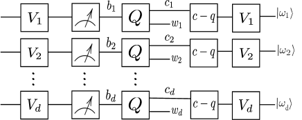
Figure 1: The procedure for creating the shadow of the samples. Here, $c-q$ means the classical to quantum mapping.

Note that given each input state, several copies of the quantum shadows can be generated, since $b^{\Phi}_{j}$ are classical. Hence, QSS can be used to estimate the loss gradient in the training procedure. For that, we proceed by using the quantum shadows for the estimation of multiple observables’ expected outcomes.

Let $\mathcal{M}_{1},\mathcal{M}_{2},\cdots,\mathcal{M}_{m}$ be $m$ observables. Suppose $n$ quantum samples $\ket{\phi_{i}},i\in[n]$ are drawn from a distribution $D$. Let $\Phi=\mathbb{E}_{D}[\outerproduct{\phi}{\phi}]$ denote the expected mixed state of the samples. The objective is to estimate the expected value of each observable $\langle\mathcal{M}_{\ell}\rangle_{\Phi}$. For that, we apply QSS on each $\ket{\phi_{i}}$ and generate $m$ shadow samples ${\hat{\Phi}_{i}}^{\operatorname*{\otimes}m}$ with the weight $\hat{w}_{i}$. Then, we measure each copy ${\hat{\Phi}_{i}}$ with one of the $m$ measurements. Let $b_{\ell,i}$ denote the outcome of the $\mathcal{M}_{\ell}$ on the shadow of the $j$th sample. Then, we apply the following estimator:

$$\widehat{\langle\mathcal{M}_{\ell}\rangle}_{\Phi}:=\frac{3^{d}}{n}\sum_{i=1}^{n}\hat{w}_{i}b_{\ell,i}.$$ (8)

We show that this is an unbiased estimate.

Theorem 2.

Given the observables $\mathcal{M}_{1},\mathcal{M}_{2},\cdots,\mathcal{M}_{m}$, and the samples $\ket{\phi_{i}},i\in[n]$, the estimates $\widehat{\langle\mathcal{M}_{\ell}\rangle}_{\Phi}$ as in (8) are unbiased, that is $\mathbb{E}[\widehat{\langle\mathcal{M}_{\ell}\rangle}_{\Phi}]=\langle\mathcal{M}_{\ell}\rangle_{\Phi}$.

The proof is provided in Appendix C. Note that the factor $3^{d}$ can be improved by using the median of the means estimator as in (Huang, Kueng, and Preskill 2020). However, for this work, the average estimator is sufficient. Moreover, it can be reduced to $3^{K}$ if the observables are local with $K$ qubit width.

Quantum shadow gradient descent

We use QSS to measure the gradient of the loss by applying it to each input sample. With this procedure, Lemma 1, and Theorem 1, we can estimate all the derivatives of the loss.

We generate the shadow samples at each iteration and pass them through the ansatz. Let $\hat{\rho}_{l}^{out}$ be the output of the ansatz at layer $l$ when the input is the shadow $\hat{\rho}$. Then, we obtain the derivatives of the gradient via a gradient measurement as in (Heidari, Grama, and Szpankowski 2022) using (10) (for product ansatz) or (6) (for non-product ansatz) but with $\hat{\rho}_{l}^{out}$ replacing ${\rho}_{l}^{out}$. Continuing this for all the layers, we obtain the shadow gradient for the current sample denoted by $\widehat{\nabla\mathcal{L}}(\overrightarrow{a},\hat{\rho}^{out}_{t},y)$. With this procedure, we apply the following update rule:

$$\overrightarrow{a}^{(t+1)}=\overrightarrow{a}^{(t)}-\eta_{t}\widehat{\nabla\mathcal{L}}(\overrightarrow{a},\hat{\rho}^{out}_{t},y_{t}).$$ (9)

From this, we obtain our shadow QGD process, which is summarized in Alg. 1.

Input: Training data $\{(\ket{\phi_{t}},y_{t})\}_{t=1}^{n}$, Learning rate $\eta_{t}$

1 Initialize $\overrightarrow{a}^{(1)}$ by randomly selecting its elements from $[-1,1]$.

2 for $t=1$ to $n$ do

3       Apply QSS on $\ket{\phi_{t}}$ to generate $\hat{\Phi}_{t}$ and $\hat{w}_{t}$ as in (7).

4       Let $\hat{\rho}_{l}^{out}$ be the output of the ansatz at layer $l$ when the input is $\hat{\Phi}_{t}$.

5       Apply the gradient measurement to obtain the raw derivatives as in (10).

6       Apply the correction terms (for non-product ansatz) using (6) to get the shadow gradient as $\widehat{\nabla\mathcal{L}}$.

7       Apply the update rule

$$\overrightarrow{a}^{(t+1)}=\overrightarrow{a}^{(t)}-\eta_{t}\widehat{\nabla\mathcal{L}}(\overrightarrow{a},\hat{\rho}^{out}_{t},y_{t}).$$

8      

9return $\overrightarrow{a}^{(n+1)}$

Algorithm 1 Shadow QSGD

Convergence analysis

One can prove the convergence of our approach using the standard analysis of stochastic gradient descent and the fact that the estimated gradient is unbiased. Conventional approaches require assumptions on the objective function $\mathcal{L}(\overrightarrow{a})$ being convex or strong-convex. However, $\mathcal{L}$ does not necessarily satisfy these conditions. For that, we present the following result based on (Bottou, Curtis, and Nocedal 2016, Lemma 4.4).

Theorem 3.

Suppose $\absolutevalue{\ell(y,\hat{y})}\leq\gamma$ is bounded, and the step sizes (learning rate) $\eta_{t}$ converge to zero as $t$ grows. Then iterations of QSGD satisfies:

$$\mathbb{E}[\mathcal{L}(\overrightarrow{a}^{(t+1)})]-\mathcal{L}(\overrightarrow{a}^{(t)})\leq-\eta_{t}\norm{\nabla\mathcal{L}(\overrightarrow{a}^{(t)})}_{2}^{2}+\frac{1}{2}L\eta^{2}_{t}c^{2},$$

where the expectation is taken with respect to the randomness in subgradient generation in QSGD, $c$ is the number of parameters, and $L>0$ is the Lipschitz constant of $\mathcal{L}(\overrightarrow{a})$.

Note that for sufficiently large $t$, the first term, which is negative, can dominate the right-hand side. Hence, $\mathcal{L}(\overrightarrow{a}^{(t)})$ can reduce in expectation. Moreover, $\mathcal{L}$ is Lipschitz continuous when $\ell$ is bounded.

4 Numerical Experiments

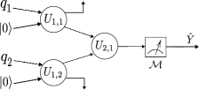
Figure 2: The QNN setup for Exp. 1.

We present experimental results in support of our theoretical claims of accuracy and performance. In each of the comparisons, we use three gradient-based methods: (i) exact gradient computation; (ii) randomized QSGD; and (iii) shadow QGD. Each experiment consists of an ansatz with a quantum dataset for the task of classification and training. The setup of each experiment is described below.

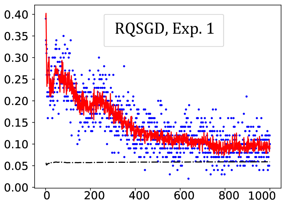
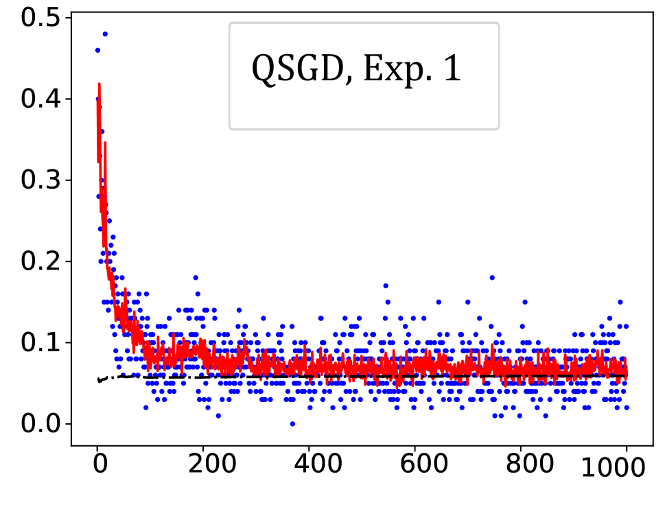
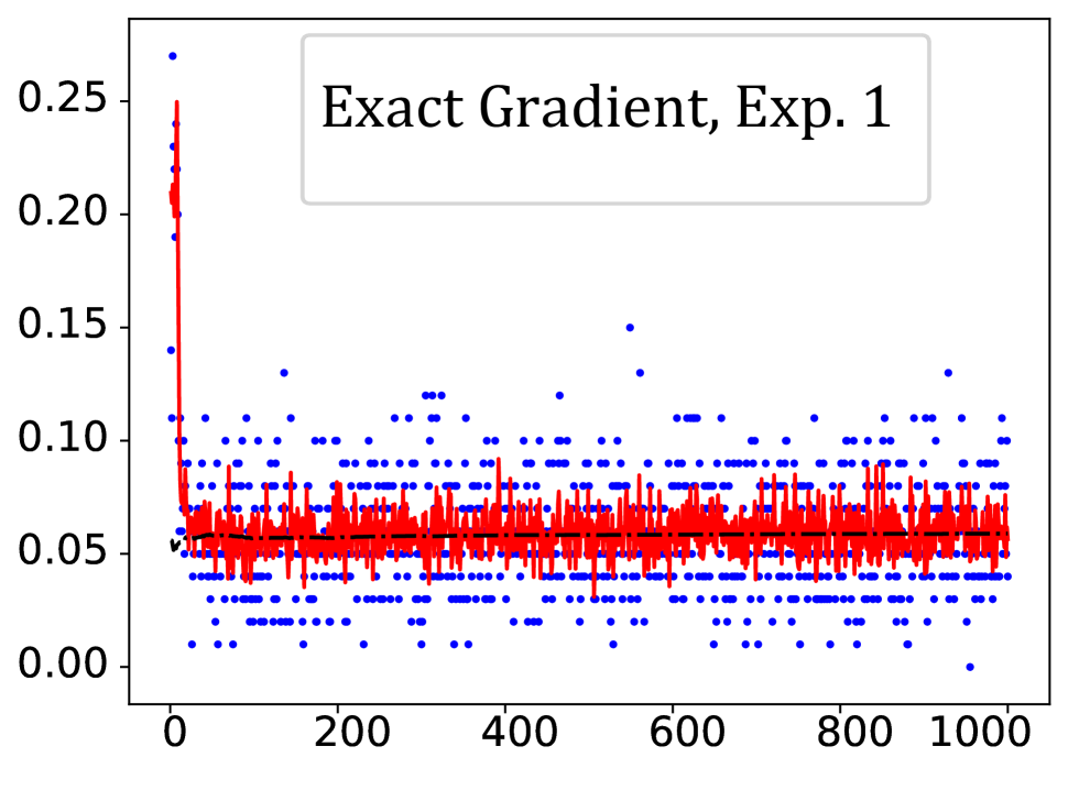
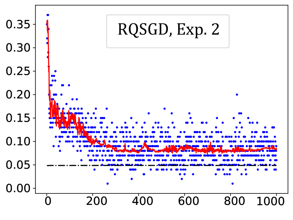
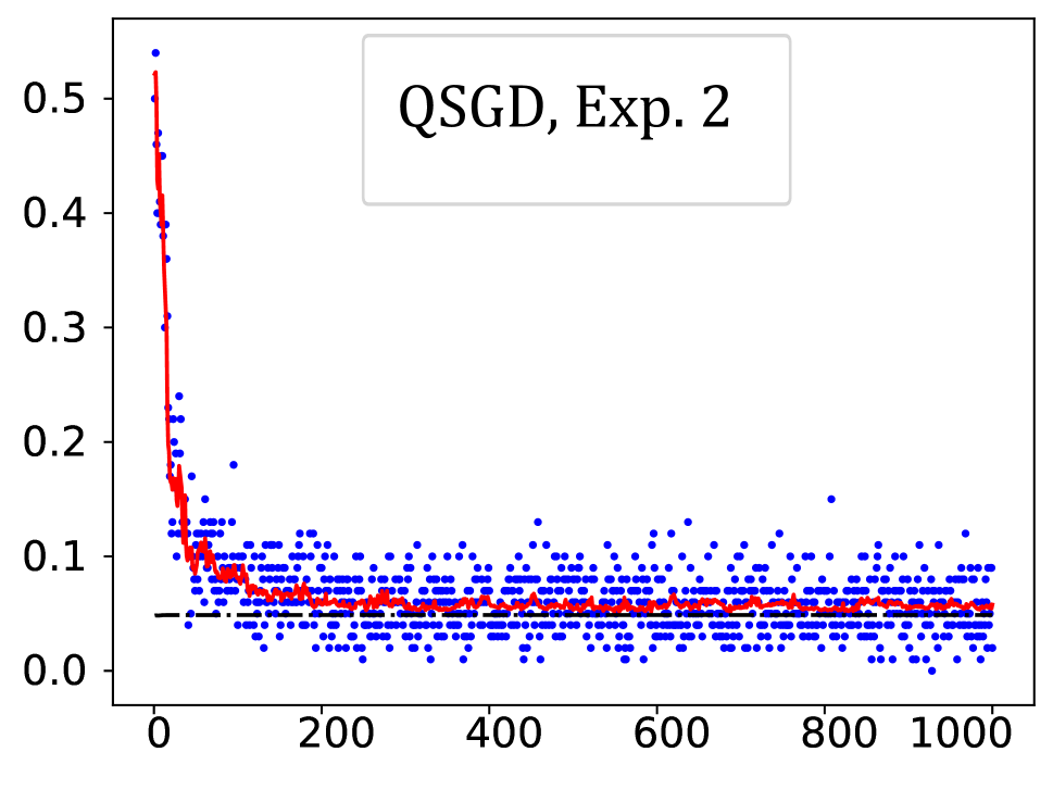
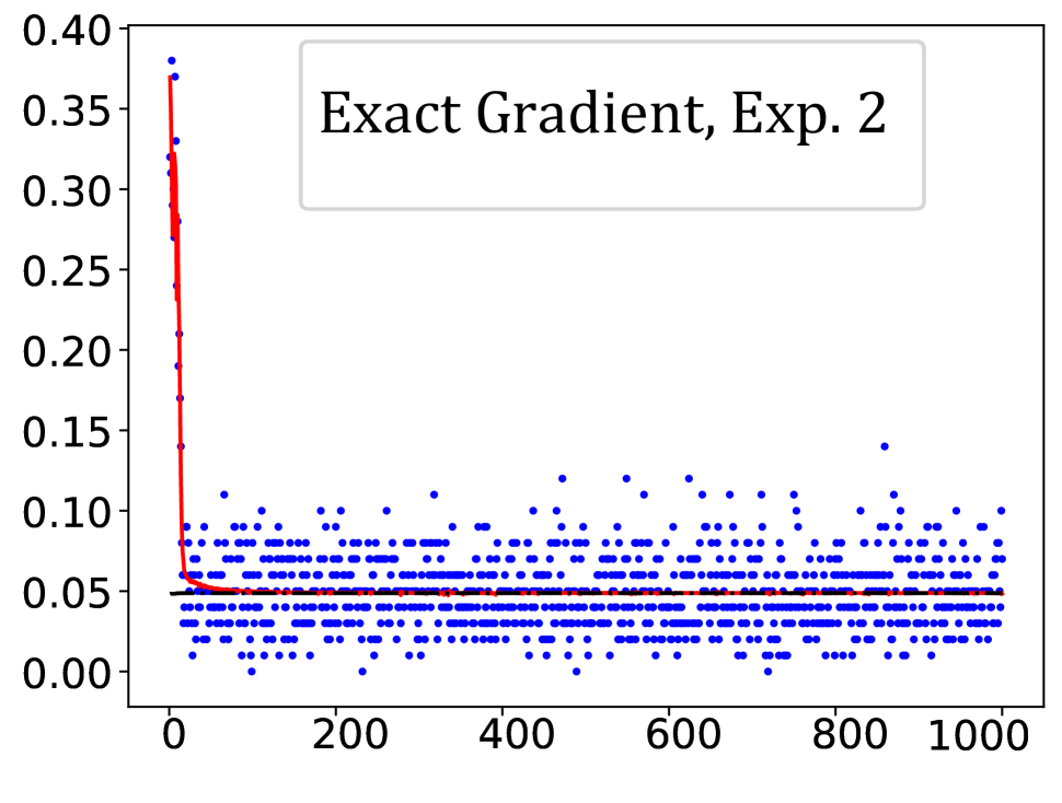
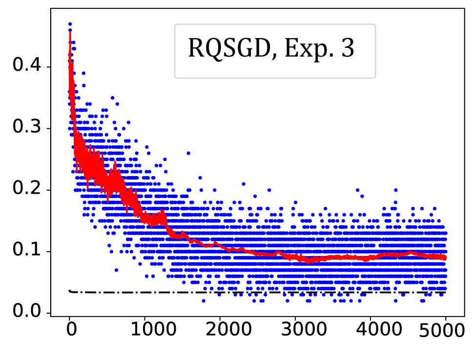
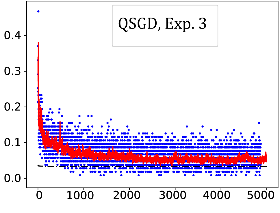
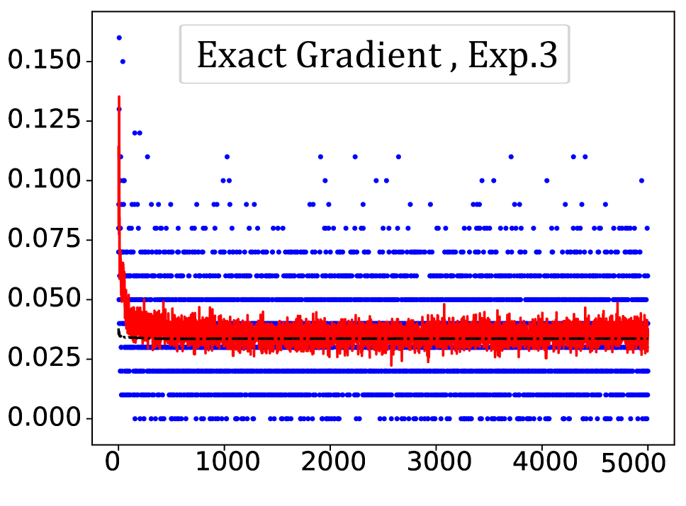
Figure 3: Comparing the training loss in three experiments based on three methods: QSGD (this work), RQSGD (Heidari, Grama, and Szpankowski 2022), and the ideal method using the exact gradient computation. The vertical axis is the training loss and the horizontal line is the training batches each containing 100 samples. The solid red lines are the expected loss, the blue dots are the empirical loss, and the black dashed line is the theoretical lower bound on the loss based on the Holevo-Helstrom theorem (Holevo 2012).

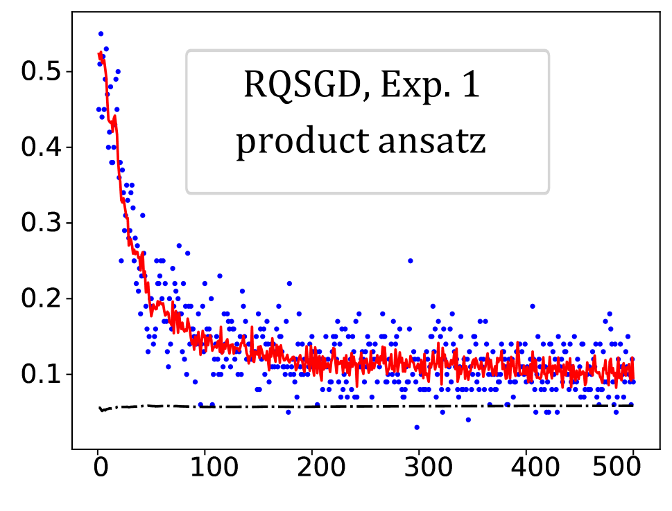
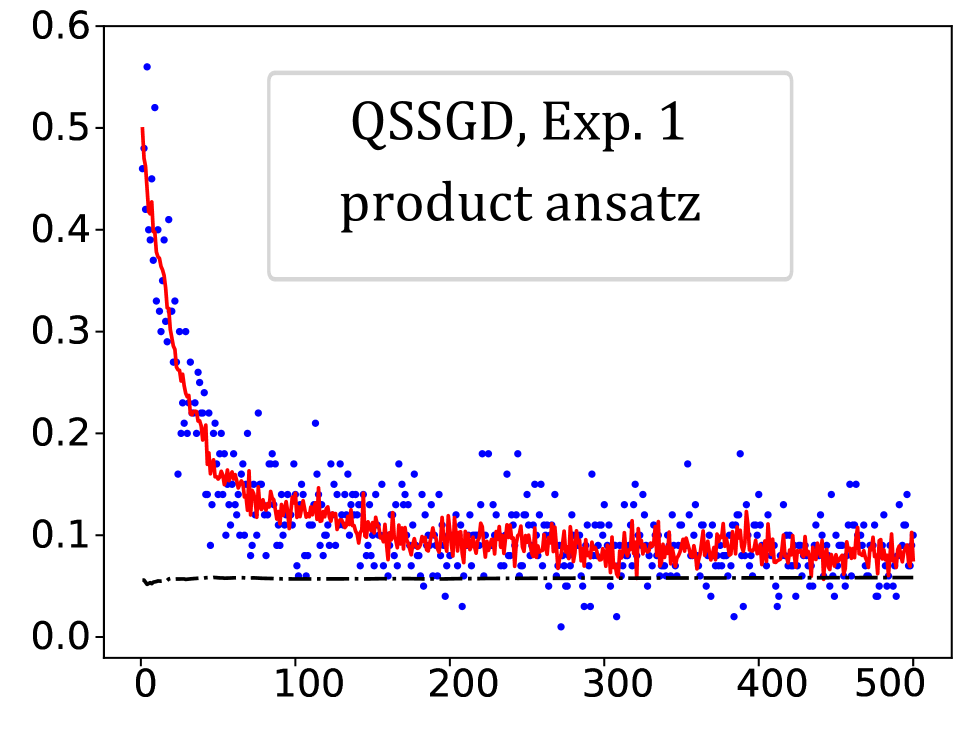
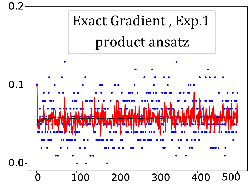
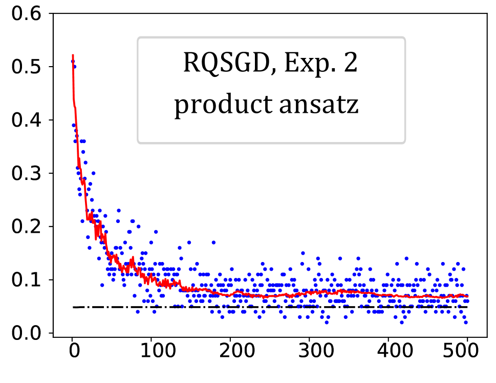
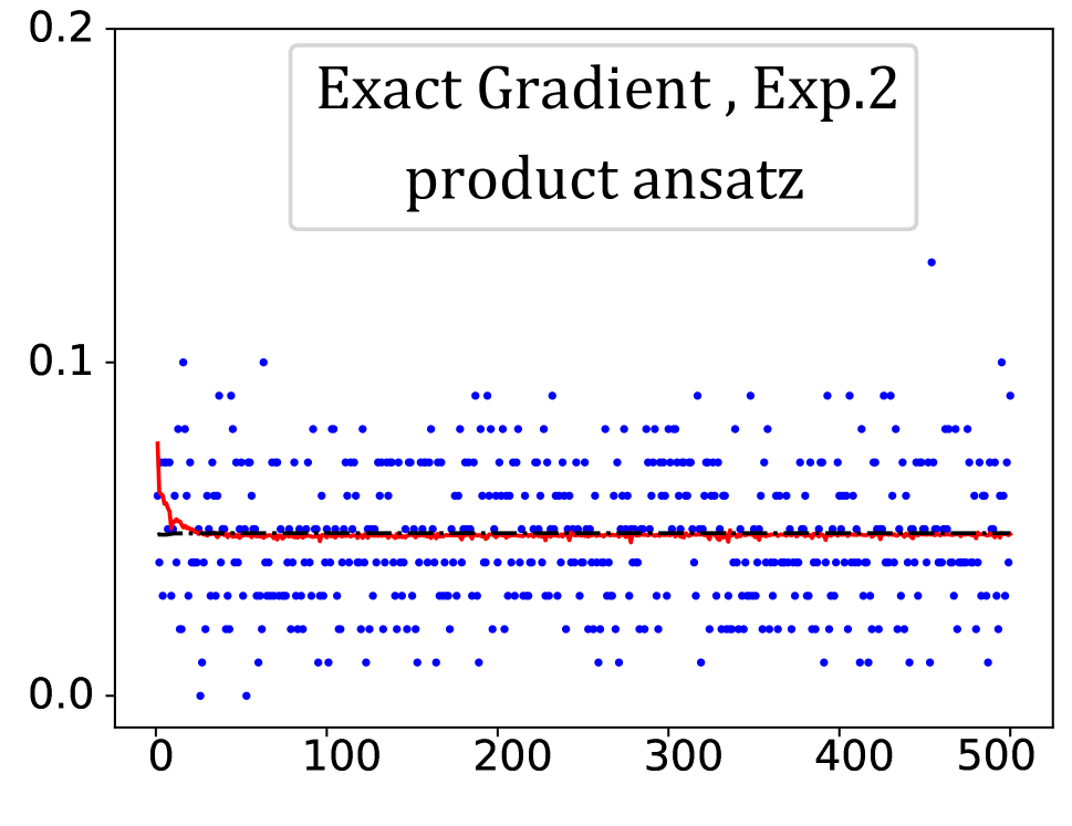
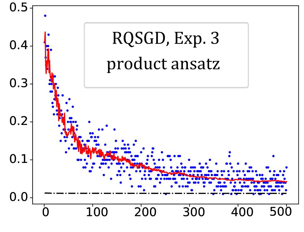
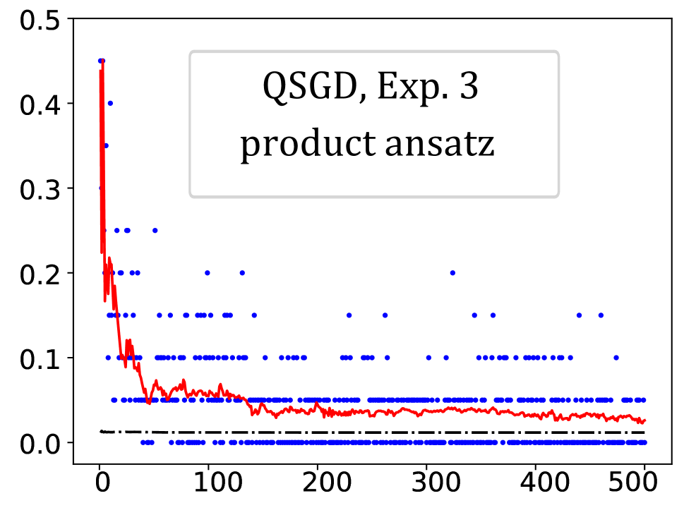
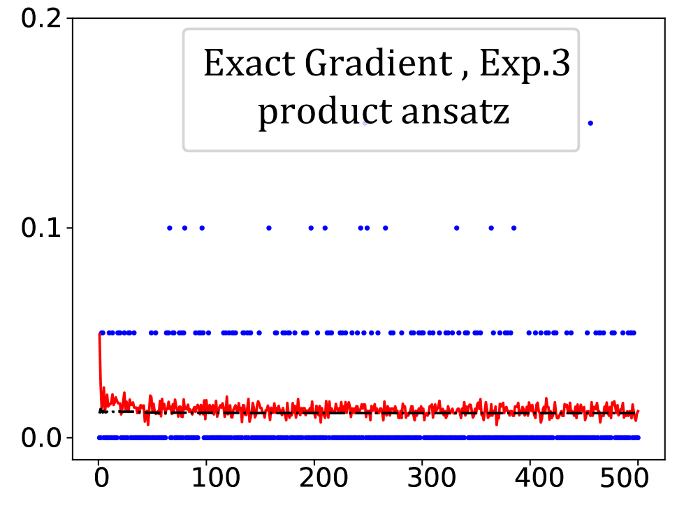
Figure 4: The training loss comparison as in Fig. 3 but with product ansatz.

Experiment 1.

The dataset is synthetically created from recent results in quantum state discrimination (Mohseni, Steinberg, and Bergou 2004; Chen et al. 2018; Patterson et al. 2021; Li, Song, and Wang 2021). It consists of two types of quantum states with dimensionality $2^{2}$. For any $u,v\in[0,1]$, the two states are defined as:

$$\rho_{1}(u) :=\outerproduct{\phi_{u}}{\phi_{u}},$$

$$\rho_{2}(v) :=\frac{1}{2}\Big{(}\outerproduct{\phi_{+v}}{\phi_{+v}}+\outerproduct{\phi_{-v}}{\phi_{-v}}\Big{)},$$

where $\ket{\phi_{u}}:=\sqrt{1-u^{2}}\ket{00}+u\ket{10},$ and $\ket{\phi_{\pm v}}:=\pm\sqrt{1-v^{2}}\ket{01}+v\ket{10}$. To generate each sample, we select $\rho_{1}$ with probability $p=1/3$ and $\rho_{2}$ with probability $(1-p)=2/3$. Moreover, for each sample, $u$ and $v$ are selected randomly, independently, and uniformly from $[0,1]^{2}$. For the labeling, we assign $y=-1$ if $\rho_{1}$ is selected; otherwise we set $y=1$. Hence, the $i$th training sample is one of the two forms: $(\rho_{1}(u_{i}),y_{i}=-1)$ or $(\rho_{2}(v_{i}),y_{i}=-1)$.

Experiment 2.

This dataset is procedurally generated to classify between separable and maximally entangled states. To do this, we randomly generate several $2$-qubit density operators of the two different types. Separable states are of the form $\rho_{A}\operatorname*{\otimes}\rho_{B}$, where $\rho_{A}$ and $\rho_{B}$ each are single-qubit density operators ($2\times 2$ matrices) generated randomly based on a Haar measure using RandomDensityMatrix in (Johnston 2016). Each maximally entangled state is of the form $\ket{\psi}:=\frac{1}{4}(\ket{00}+\ket{01}+\ket{10}+\ket{11}).$ For the labeling, we assign $y=-1$ to separable states and $y=1$ to maximally entangled states.

Experiment 3.

For testing the performance of our approach in higher dimension ($\dim=2^{4}$), we classify multi-qubits Greenberger-Horne-Zeilinger (GHZ) states (with label $y=1$) from the separable states (with label $y=-1$). The GHZ state for multi-qubits is a generalization of the three-qubit GHZ state. It is a type of entangled quantum state that involves multiple qubits and exhibits non-local correlations. We consider $4$-qubit GHZ state given by $\ket{GHZ}=\frac{\ket{0000}+\ket{1111}}{\sqrt{2}}.$ The separable states are generated in the same manner as Experiment 2.

Dataset	QSGD	RQSGD	Exact	Up. bound	QSGD	RQSGD	Exact	Up. bound
Exp. 1	93.10 %	90.22 %	93.76 %	93.81 %	91.20 %	89.38 %	93.78 %	93.81 %
Exp. 2	94.32 %	91.68 %	95.14 %	95.16%	93.51 %	93.13 %	95.13 %	95.16%
Exp. 3	93.82 %	90.78 %	96.25 %	96.45 %	97.34 %	93.55 %	98.67 %	98.78 %

Table 1: Validation accuracy of the trained ansatz for the product (right) and non-product (left) forms.

Ansatz:

For Experiments 1 and 2, we use a QNN as the ansatz (see Fig. 2). This QNN is composed of three perceptions, where $U_{11},U_{12},U_{21}$ are parameterized unitary operators either of the form $\exp\{i\sum_{\mathbf{s}}b_{\mathbf{s}}\sigma^{\mathbf{s}}\},$ or the product $\prod_{\mathbf{s}}\exp\{ib_{\mathbf{s}}\sigma^{\mathbf{s}}\},$ where $\mathbf{s}\in\left\{0,1,2,3\right\}^{2}$. Hence, there are $c=48$ parameters to be trained. The inputs are $2$-qubit states with two ancilla qubits $\ket{00}$. The measurement performed on the readout qubits is the POVM $\mathcal{M}:=\{\Pi_{-1},\Pi_{1}\}$ with outcomes in $\{-1,1\}$ and operators $\Pi_{-1}=I_{2}-\Pi_{1}=\outerproduct{00}{00}+\outerproduct{11}{11},$ where $I_{2}$ is the $2$-qubit identity.

For the GHZ dataset, the ansatz is $16\times 16$ unitary operator parameterized either as

$$\exp\{i\sum_{\mathbf{s}\in\left\{0,1,2,3\right\}^{4}}a^{\prime}_{\mathbf{s}}\sigma^{\mathbf{s}}\big{\}},$$

or the product form $\prod_{\mathbf{s}}\exp\{ib_{\mathbf{s}}\sigma^{\mathbf{s}}\}.$ Hence, there are $c^{\prime}=4^{4}=256$ parameters for training. The output state is measured as POVM $\mathcal{M}^{\prime}:=\{\Pi^{\prime}_{-1},\Pi^{\prime}_{1}\}$, with outcomes in $\{-1,1\}$ and operators defined as:

$$\Pi^{\prime}_{-1}=I_{4}-\Pi^{\prime}_{1}=\outerproduct{0000}{0000}+\outerproduct{1111}{1111},$$

where $I_{4}$ is the $4$-qubit identity.

Experimental Results

Each experiment has two versions, the product and non-product ansatz. We train the corresponding ansatz using three different methods: (i) our proposed QSGD, (ii) Randomized QSGD (Heidari, Grama, and Szpankowski 2022), and (iii) the ideal training procedure when the gradient is known exactly. Fig. 3 presents the training loss, for non-product ansatz, as a function of batch number for each method across the three datasets. Fig. 4 is the same figure but with product ansatzes. We also included a theoretical lower bound based on the Holevo-Holstrom theorem (Holevo 2012).

The figure supports the following claims: the convergence of QSGD is significantly faster than RQSGD, and is comparable to the exact gradient execution. We do note a slight loss in performance w.r.t. the latter – this degradation is due to the approximations introduced into gradient computation, as opposed to an exact gradient. We also generated a validation set of 2000 samples to test and compare the training procedures’ accuracy. These results are summarized in Table 1. The upper bound is again based on the Holevo-Holstrom theorem. From Table 1, we note that the accuracy of QSGD is significantly better than Randomized QSGD and close to the ideal method with an exact gradient. All experiments are simulated in a classical computer.

Conclusion

We proposed a novel quantum shadow sampling technique to rapidly estimate quantum states while being consistent with the no-cloning postulate. Our one-shot method takes quantum states as input and produces several shadows for each state. We use the shadows to approximate the gradient of the loss with respect to the ansatz parameters. Based on our shadowing procedure, we proposed a novel update rule called quantum shadow gradient descent. We proved that our method has convergence guarantees. Moreover, we characterized the gradient of non-product ansatz in terms of that of products but with correction terms. In summary, we presented a novel gradient-based update that is one-shot, has a fast convergence rate and is applicable to non-product ansatzes. We supported all our theoretical claims with experimental verification.

Appendix A Proof of Lemma 1

Lemma 1.

Let ${\rho}_{l}^{out}=U_{\leq l}\rho U_{\leq l}^{\dagger}$ denote the density operator of the output state at layer $l$ when the input is $\rho$. Then, the derivative of the loss is given by:

$$\frac{\partial\mathcal{L}(a_{\mathbf{s}},\ket{\phi},y)}{\partial a_{\mathbf{s}_{l}}}=\sum_{\hat{y}}i\ell(y,\hat{y})\tr{M_{\hat{y}}U_{>l}\big{[}\sigma^{\mathbf{s}_{l}},{\rho}_{l}^{out}\big{]}U^{\dagger}_{>l}},$$ (10)

where $[\cdot,\cdot]$ is the commutator operation and $y$ is the label of $\rho$.

Proof.

The lemma follows from the same argument as in (Heidari, Grama, and Szpankowski 2022). For completeness, we provide the proof. The linearity of the derivatives yields the following:

$$\frac{\partial\mathcal{L}(\overrightarrow{a},\ket{\phi_{t}},y_{t})}{\partial a_{\mathbf{s}_{l}}}=\sum_{\hat{y}}\ell(y_{t},\hat{y})\tr\{M_{\hat{y}}\frac{\partial}{\partial a_{\mathbf{s}_{l}}}\Big{(}U(\overrightarrow{a})\outerproduct{\phi_{t}}{\phi_{t}}U^{\dagger}(\overrightarrow{a})\Big{)}\Big{\}}.$$

Note that $U(\overrightarrow{a})=U_{>l}U_{\leq l}$. Hence, the derivative only acts on the first $l$ layers. For that, $\frac{\partial}{\partial a_{\mathbf{s}_{l}}}U=iU_{>l}\sigma^{\mathbf{s}_{l}}U_{\leq l}$. Hence, the derivative inside the trace is given by:

$$i\Big{(}U_{>l}\sigma^{\mathbf{s}_{l}}U_{\leq l}\outerproduct{\phi_{t}}{\phi_{t}}U^{\dagger}-U\outerproduct{\phi_{t}}{\phi_{t}}U_{\leq l}^{\dagger}\sigma^{\mathbf{s}_{l}}U_{>l}^{\dagger}\Big{)}.$$

Denote ${\rho}_{l}^{out}=U_{\leq l}\rho U_{\leq l}^{\dagger}$ as the output state. Then, the above term can be written as the commutator $U_{>l}\big{[}\sigma^{\mathbf{s}_{l}},{\rho}_{l}^{out}\big{]}U_{>l}^{\dagger}$. With this, the expression in the lemma is obtained. ∎

Appendix B Proof of Theorem 1

Theorem 1.

For a non-prodct ansatz $U(\overrightarrow{a})$ as in (5), let $\rho^{out}$ be the output state. For any $\mathbf{t}\in\left\{0,1,2,3\right\}^{d}$, define $\frac{\partial\tilde{\mathcal{L}}}{\partial a_{\mathbf{t}}}:=\sum_{\hat{y}}i\ell(y,\hat{y})\tr{M_{\hat{y}}\big{[}\sigma^{\mathbf{t}},{\rho}^{out}\big{]}}$, where $y$ is the true label. Then, the derivative of the loss for the non-product $U$ expands in terms of $\frac{\partial\tilde{\mathcal{L}}}{\partial a_{\mathbf{t}}}$ as:

$$\frac{\partial\mathcal{L}}{\partial a_{\mathbf{s}}}=\frac{\partial\tilde{\mathcal{L}}}{\partial a_{\mathbf{s}}}+\sum_{\mathbf{r},\mathbf{t}}{a}_{\mathbf{r}}(\kappa_{\mathbf{r}\mathbf{s}\mathbf{t}}-\kappa_{\mathbf{s}\mathbf{r}\mathbf{t}})\frac{\partial\tilde{\mathcal{L}}}{\partial a_{\mathbf{t}}}+\frac{1}{3}\sum_{\mathbf{r},\mathbf{q},\mathbf{r}^{\prime},\mathbf{t}}a_{\mathbf{r}}a_{\mathbf{r}^{\prime}}\kappa_{\mathbf{r}\mathbf{s}\mathbf{q}}\kappa_{\mathbf{q}\mathbf{r}^{\prime}\mathbf{t}}\frac{\partial\tilde{\mathcal{L}}}{\partial a_{\mathbf{t}}},\qquad\forall\mathbf{s}\in\left\{0,1,2,3\right\}^{d}.$$

Proof.

Let $W_{n}:=\prod_{\mathbf{s}}\exp{i\frac{a_{\mathbf{s}}}{n}\sigma^{\mathbf{s}}}.$ Then from Theorem 3 of (Suzuki 1976),

$$U(\overrightarrow{a})=\lim_{n\rightarrow\infty}W_{n}^{n}.$$

The derivative of the loss with respect to $a_{\mathbf{s}}$ is

$$\frac{\partial\mathcal{L}}{\partial a_{\mathbf{s}}}=\sum_{\hat{y}}\ell(y,\hat{y})\tr{M_{\hat{y}}\frac{\partial}{\partial a_{\mathbf{s}}}\Big{(}U(\overrightarrow{a})\rho U^{\dagger}(\overrightarrow{a})\Big{)}}.$$

Since the derivative of $W_{n}$ is a converging sequence, we can interchange limit with the derivative. operator:

$$\frac{\partial\mathcal{L}}{\partial a_{\mathbf{s}}}=\lim_{n\rightarrow\infty}\sum_{\hat{y}}\ell(y,\hat{y})\tr{M_{\hat{y}}\frac{\partial}{\partial a_{\mathbf{s}}}\Big{(}W_{n}^{n}\rho W_{n}^{n\dagger}\Big{)}}.$$

Consider an ordering of the elements of $\left\{0,1,2,3\right\}^{d}$ and define the following operators

$$W_{\leq\mathbf{s}}:=\prod_{\mathbf{s}^{\prime}<\mathbf{s}}\exp{i\frac{a_{\mathbf{s}^{\prime}}}{n}\sigma^{\mathbf{s}^{\prime}}},\qquad W_{\geq\mathbf{s}}:=\prod_{\mathbf{s}^{\prime}\geq\mathbf{s}}\exp{i\frac{a_{\mathbf{s}^{\prime}}}{n}\sigma^{\mathbf{s}^{\prime}}}$$

With this notation, the derivative of $W_{n}$ equals to the following

$$\tilde{W}_{n}:=\frac{\partial W_{n}}{\partial a_{\mathbf{s}}}=\frac{i}{n}W_{<\mathbf{s}}\sigma^{\mathbf{s}}W_{\geq\mathbf{s}}$$

Then the derivative of $W_{n}^{n}$ equals to

$$\frac{\partial W_{n}}{\partial a_{\mathbf{s}}}=\sum_{k=0}^{n-1}W_{n}^{k}\tilde{W}W_{n}^{n-k-1}.$$

As a result, we have that

$$\frac{\partial}{\partial a_{\mathbf{s}}}\Big{(}W_{n}^{n}\rho W_{n}^{n\dagger}\Big{)} =\Big{(}\frac{\partial W_{n}^{n}}{\partial a_{\mathbf{s}}}\Big{)}\rho W_{n}^{n\dagger}+W_{n}^{n}\rho\Big{(}\frac{\partial W_{n}^{n\dagger}}{\partial a_{\mathbf{s}}}\Big{)}$$

$$=\sum_{k}W_{n}^{k}\tilde{W}W_{n}^{n-k-1}\rho W_{n}^{n\dagger}-\sum_{k}W_{n}^{n}\rho W_{n}^{k\dagger}\tilde{W}^{\dagger}W_{n}^{n-k-1\dagger}$$

$$=\sum_{k}W_{n}^{k}\tilde{W}W_{n}^{n-k-1}\rho W_{n}^{n\dagger}-W_{n}^{n}\rho W_{n}^{n-k-1\dagger}\tilde{W}^{\dagger}W_{n}^{k\dagger},$$

where the last inequality follows by changing $k$ to $n-k-1$ in the second summation. Let $\rho_{n}^{out}:=W_{n}^{n}\rho W_{n}^{n\dagger}$. Then, from the above expression and by noting that $W_{n}^{k+1}W_{n}^{k+1\dagger}=I$ we have that

$$\frac{\partial}{\partial a_{\mathbf{s}}}\Big{(}W_{n}^{n}\rho W_{n}^{n\dagger}\Big{)} =\sum_{k}W_{n}^{k}\tilde{W}W_{n}^{k+1\dagger}\rho_{n}^{out}-\rho_{n}^{out}W_{n}^{k+1}\tilde{W}^{\dagger}W_{n}^{k\dagger},$$

Define $A_{n,k}:=W_{n}^{k}W_{<\mathbf{s}}$. Then, we have that

$$W_{n}^{k}\tilde{W}W_{n}^{k+1\dagger} =\frac{i}{n}W_{n}^{k}W_{<\mathbf{s}}\sigma^{\mathbf{s}}W_{\geq\mathbf{s}}W_{n}^{k+1\dagger}$$

$$=A_{n,k}\sigma^{\mathbf{s}}A_{n,k}^{\dagger}.$$

As a result the above derivative equals to

$$\frac{\partial\mathcal{L}}{\partial a_{\mathbf{s}}}=\lim_{n\rightarrow\infty}\frac{i}{n}\sum_{\hat{y}}\ell(y,\hat{y})\sum_{k}\tr{M_{\hat{y}}[A_{n,k}\sigma^{\mathbf{s}}A_{n,k}^{\dagger},\rho_{n}^{out}]}.$$ (11)

Next, we apply Taylor’s approximation as

$$\exp{i\frac{a_{\mathbf{s}^{\prime}}}{n}\sigma^{bfs^{\prime}}}=I+i\frac{a_{\mathbf{s}^{\prime}}}{n}\sigma^{\mathbf{s}^{\prime}}+\order{\frac{1}{n^{2}}}.$$

Then, we can write

$$W_{n}=\prod_{\mathbf{s}^{\prime}}\Big{(}I+i\frac{a_{\mathbf{s}^{\prime}}}{n}\sigma^{\mathbf{s}^{\prime}}+\order{\frac{1}{n^{2}}}\Big{)}=I+i\sum_{\mathbf{s}^{\prime}}\frac{a_{\mathbf{s}^{\prime}}}{n}\sigma^{\mathbf{s}^{\prime}}+\order{\frac{c}{n^{2}}},$$

where $c$ is the number of the parameters $a_{\mathbf{s}}$, and we used the fact that $\sum_{\mathbf{s}}|a_{\mathbf{s}}|^{2}=O(c)$. Rising both sides to the power $k$ and using the inequality $(1+x)^{k}=1+kx+O(x^{2})$ on the right-hand side give

$$W^{k}_{n}=I+ik\sum_{\mathbf{s}^{\prime}}\frac{a_{\mathbf{s}^{\prime}}}{n}\sigma^{\mathbf{s}^{\prime}}+\order{\frac{kc}{n^{2}}}.$$

Similarly, using the Taylor;s expansion for each term in $W_{<\mathbf{s}}$, we get

$$W_{<\mathbf{s}}=I+\frac{i}{n}\sum_{\mathbf{s}^{\prime\prime}<\mathbf{s}}a_{\mathbf{s}^{\prime\prime}}\sigma^{\mathbf{s}^{\prime\prime}}+\order{\frac{c}{n^{2}}}.$$

Therefore, we can write $A_{n,k}$ as

$$A_{n,k}=W_{n}^{k}W_{<\mathbf{s}} =I+\frac{ik}{n}\sum_{\mathbf{s}^{\prime}}a_{\mathbf{s}^{\prime}}\sigma^{\mathbf{s}^{\prime}}+\frac{i}{n}\sum_{\mathbf{s}^{\prime\prime}<\mathbf{s}}a_{\mathbf{s}^{\prime\prime}}\sigma^{\mathbf{s}^{\prime\prime}}+\order{\frac{kc}{n^{2}}}.$$

Consequently, we have that

$$A_{n,k}\rho_{n}^{out}A_{n,k}^{\dagger} =\sigma^{\mathbf{s}}+\frac{ik}{n}\sum_{\mathbf{s}^{\prime}}a_{\mathbf{s}^{\prime}}\sigma^{\mathbf{s}^{\prime}}\sigma^{\mathbf{s}}+\frac{i}{n}\sum_{\mathbf{s}^{\prime\prime}<\mathbf{s}}a_{\mathbf{s}^{\prime\prime}}\sigma^{\mathbf{s}^{\prime\prime}}\sigma^{\mathbf{s}}-\frac{ik}{n}\sum_{\mathbf{s}^{\prime}}a_{\mathbf{s}^{\prime}}\sigma^{\mathbf{s}}\sigma^{\mathbf{s}^{\prime}}-\frac{i}{n}\sum_{\mathbf{s}^{\prime\prime}<\mathbf{s}}a_{\mathbf{s}^{\prime\prime}}\sigma^{\mathbf{s}}\sigma^{\mathbf{s}^{\prime\prime}}$$

$$+\frac{k^{2}}{n^{2}}\sum_{\mathbf{s}^{\prime},\mathbf{r}^{\prime}}a_{\mathbf{s}^{\prime}}a_{\mathbf{r}^{\prime}}\sigma^{\mathbf{s}^{\prime}}\sigma^{\mathbf{s}}\sigma^{\mathbf{r}^{\prime}}+\frac{1}{n^{2}}\sum_{\mathbf{s}^{\prime\prime},\mathbf{r}^{\prime\prime}<\mathbf{s}}a_{\mathbf{s}^{\prime\prime}}a_{\mathbf{r}^{\prime\prime}}\sigma^{\mathbf{s}^{\prime\prime}}\sigma^{\mathbf{s}}\sigma^{\mathbf{r}^{\prime\prime}}$$

$$+\frac{k}{n^{2}}\sum_{\begin{subarray}{c}\mathbf{s}^{\prime}\\ \mathbf{r}^{\prime\prime}<\mathbf{s}\end{subarray}}a_{\mathbf{s}^{\prime}}a_{\mathbf{r}^{\prime\prime}}\sigma^{\mathbf{s}^{\prime}}\sigma^{\mathbf{s}}\sigma^{\mathbf{r}^{\prime\prime}}+\frac{k}{n^{2}}\sum_{\begin{subarray}{c}\mathbf{s}^{\prime\prime}<\mathbf{s},\\ \mathbf{r}^{\prime}\end{subarray}}a_{\mathbf{s}^{\prime\prime}}a_{\mathbf{r}^{\prime}}\sigma^{\mathbf{s}^{\prime\prime}}\sigma^{\mathbf{s}}\sigma^{\mathbf{r}^{\prime}}+\order{\frac{kc}{n^{2}}}.$$

Note that the third, fifth, seventh, eighth and ninth are bounded be a corresponding big-O notation as

$$A_{n,k}\rho_{n}^{out}A_{n,k}^{\dagger} =\sigma^{\mathbf{s}}+\frac{ik}{n}\sum_{\mathbf{s}^{\prime}}a_{\mathbf{s}^{\prime}}\sigma^{\mathbf{s}^{\prime}}\sigma^{\mathbf{s}}+\order{\frac{c}{n}}-\frac{ik}{n}\sum_{\mathbf{s}^{\prime}}a_{\mathbf{s}^{\prime}}\sigma^{\mathbf{s}}\sigma^{\mathbf{s}^{\prime}}+\order{\frac{c}{n}}$$

$$+\frac{k^{2}}{n^{2}}\sum_{\mathbf{s}^{\prime},\mathbf{r}^{\prime}}a_{\mathbf{s}^{\prime}}a_{\mathbf{r}^{\prime}}\sigma^{\mathbf{s}^{\prime}}\sigma^{\mathbf{s}}\sigma^{\mathbf{r}^{\prime}}+\order{\frac{c^{2}}{n^{2}}}+\order{\frac{kc^{2}}{n^{2}}}+\order{\frac{kc^{2}}{n^{2}}}+\order{\frac{kc}{n^{2}}}$$

$$=\underbrace{\sigma^{\mathbf{s}}}_{(I)}+\underbrace{\frac{ik}{n}\sum_{\mathbf{s}^{\prime}}a_{\mathbf{s}^{\prime}}\sigma^{\mathbf{s}^{\prime}}\sigma^{\mathbf{s}}}_{(II)}-\underbrace{\frac{ik}{n}\sum_{\mathbf{s}^{\prime}}a_{\mathbf{s}^{\prime}}\sigma^{\mathbf{s}}\sigma^{\mathbf{s}^{\prime}}}_{(III)}+\underbrace{\frac{k^{2}}{n^{2}}\sum_{\mathbf{s}^{\prime},\mathbf{r}^{\prime}}a_{\mathbf{s}^{\prime}}a_{\mathbf{r}^{\prime}}\sigma^{\mathbf{s}^{\prime}}\sigma^{\mathbf{s}}\sigma^{\mathbf{r}^{\prime}}}_{(IV)}+\order{\frac{c}{n}+\frac{kc^{2}}{n^{2}}}.$$

Plugging this into (11) gives

$$\frac{\partial\mathcal{L}}{\partial a_{\mathbf{s}}}=\lim_{n\rightarrow\infty}\frac{i}{n}\sum_{\hat{y}}\ell(y,\hat{y})\sum_{k}\tr{M_{\hat{y}}[(I)+(II)+(III)+(IV),\rho_{n}^{out}]}+\Delta,$$

where $\Delta$ is the residual term given by

$$\Delta=\lim_{n\rightarrow\infty}\frac{\ell^{max}}{n}\sum_{k}\order{\frac{c}{n}+\frac{kc^{2}}{n^{2}}},$$

where used the fact that $|\ell(y,\hat{y})|\leq\ell^{max}<\infty$, and that $\sum_{\hat{y}}M_{\hat{y}}=I$ due to the POVM formulation. This residual term is equal to zero, because

$$\Delta=\lim_{n\rightarrow\infty}\frac{\ell^{max}}{n}\order{c+\frac{n(n+1)c^{2}}{2n^{2}}}=\lim_{n\rightarrow\infty}\order{\frac{\ell^{max}c}{n}+\frac{\ell^{max}(n+1)c^{2}}{2n^{2}}}=0.$$

Hence, it remains to compute the main terms.

(I):

$$\lim_{n\rightarrow\infty}\frac{i}{n}\sum_{\hat{y}}\ell(y,\hat{y})\sum_{k}\tr{M_{\hat{y}}[\sigma^{\mathbf{s}},\rho_{n}^{out}]} =\lim_{n\rightarrow\infty}i\sum_{\hat{y}}\ell(y,\hat{y})\tr{M_{\hat{y}}[\sigma^{\mathbf{s}},\rho_{n}^{out}]}$$

$$=i\sum_{\hat{y}}\ell(y,\hat{y})\tr{M_{\hat{y}}[\sigma^{\mathbf{s}},\Big{(}\lim_{n\rightarrow\infty}\rho_{n}^{out}\Big{)}]}$$

$$=i\sum_{\hat{y}}\ell(y,\hat{y})\tr{M_{\hat{y}}[\sigma^{\mathbf{s}},\rho^{out}]}=\frac{\partial\tilde{\mathcal{L}}}{\partial a_{\mathbf{s}}}$$

(II):

$$\lim_{n\rightarrow\infty} \sum_{\mathbf{s}^{\prime}}a_{\mathbf{s}^{\prime}}\sum_{\hat{y}}\ell(y,\hat{y})\sum_{k}\frac{-k}{n^{2}}\tr{M_{\hat{y}}[\sigma^{\mathbf{s}^{\prime}}\sigma^{\mathbf{s}},\rho_{n}^{out}]}=\lim_{n\rightarrow\infty}\sum_{\mathbf{s}^{\prime}}a_{\mathbf{s}^{\prime}}\sum_{\hat{y}}\ell(y,\hat{y})\frac{-n(n+1)}{2n^{2}}\tr{M_{\hat{y}}[\sigma^{\mathbf{s}^{\prime}}\sigma^{\mathbf{s}},\rho_{n}^{out}]}$$

$$=-\frac{1}{2}\sum_{\mathbf{s}^{\prime}}a_{\mathbf{s}^{\prime}}\sum_{\hat{y}}\ell(y,\hat{y})\tr{M_{\hat{y}}[\sigma^{\mathbf{s}^{\prime}}\sigma^{\mathbf{s}},\lim_{n\rightarrow\infty}\frac{(n+1)}{n}\rho_{n}^{out}]}$$

$$=-\frac{1}{2}\sum_{\mathbf{s}^{\prime}}a_{\mathbf{s}^{\prime}}\sum_{\hat{y}}\ell(y,\hat{y})\tr{M_{\hat{y}}[\sigma^{\mathbf{s}^{\prime}}\sigma^{\mathbf{s}},\rho^{out}]}.$$

Next, from the definition of $\kappa_{jk\ell}$ we can write, $\sigma^{\mathbf{s}^{\prime}}\sigma^{\mathbf{s}}=\sum_{\mathbf{t}}\kappa_{\mathbf{s}^{\prime},\mathbf{s},\mathbf{t}}\sigma^{\mathbf{t}}$. Hence, from the definition of $\frac{\partial\tilde{\mathcal{L}}}{\partial a_{\mathbf{s}}}$ the term (II) equals to $-\frac{1}{2}\sum_{\mathbf{s}^{\prime},\mathbf{t}}a_{\mathbf{s}^{\prime}}\kappa_{\mathbf{s}^{\prime},\mathbf{s},\mathbf{t}}\frac{\partial\tilde{\mathcal{L}}}{\partial a_{\mathbf{t}}}$.

(III):

This is similar to the previous part and simplifies to $\frac{1}{2}\sum_{\mathbf{s}^{\prime},\mathbf{t}}a_{\mathbf{s}^{\prime}}\kappa_{\mathbf{s},\mathbf{s}^{\prime},\mathbf{t}}\frac{\partial\tilde{\mathcal{L}}}{\partial a_{\mathbf{t}}}$.

(IV):

$$\lim_{n\rightarrow\infty} \sum_{\mathbf{s}^{\prime},\mathbf{r}^{\prime}}a_{\mathbf{s}^{\prime}}a_{\mathbf{r}^{\prime}}\sum_{\hat{y}}\ell(y,\hat{y})\sum_{k}\frac{k^{2}}{n^{2}}\tr{M_{\hat{y}}[\sigma^{\mathbf{s}^{\prime}}\sigma^{\mathbf{s}}\sigma^{\mathbf{r}^{\prime}},\rho_{n}^{out}]}$$

$$=\lim_{n\rightarrow\infty}\sum_{\mathbf{s}^{\prime},\mathbf{r}^{\prime}}a_{\mathbf{s}^{\prime}}a_{\mathbf{r}^{\prime}}\sum_{\hat{y}}\ell(y,\hat{y})\frac{n(n+1)(2n+1)}{6n^{3}}\tr{M_{\hat{y}}[\sigma^{\mathbf{s}^{\prime}}\sigma^{\mathbf{s}}\sigma^{\mathbf{r}^{\prime}},\rho_{n}^{out}]}$$

$$=\sum_{\mathbf{s}^{\prime},\mathbf{r}^{\prime}}a_{\mathbf{s}^{\prime}}a_{\mathbf{r}^{\prime}}\sum_{\hat{y}}\ell(y,\hat{y})\tr{M_{\hat{y}}[\sigma^{\mathbf{s}^{\prime}}\sigma^{\mathbf{s}}\sigma^{\mathbf{r}^{\prime}},\Big{(}\lim_{n\rightarrow\infty}\frac{(n+1)(2n+1)}{6n^{2}}\rho_{n}^{out}\Big{)}]}$$

$$=\sum_{\mathbf{s}^{\prime},\mathbf{r}^{\prime}}a_{\mathbf{s}^{\prime}}a_{\mathbf{r}^{\prime}}\sum_{\hat{y}}\ell(y,\hat{y})\tr{M_{\hat{y}}[\sigma^{\mathbf{s}^{\prime}}\sigma^{\mathbf{s}}\sigma^{\mathbf{r}^{\prime}},\rho^{out}]}.$$

Note that $\sigma^{\mathbf{s}^{\prime}}\sigma^{\mathbf{s}}\sigma^{\mathbf{r}^{\prime}}=\sum_{\mathbf{q},\mathbf{t}}\kappa_{\mathbf{s}^{\prime}\mathbf{s}\mathbf{q}}\kappa_{\mathbf{q}\mathbf{r}^{\prime}\mathbf{t}}\sigma^{\mathbf{t}}.$ Hence, the derivative related to the $(IV)$ term equals to $\frac{1}{3}\sum_{\mathbf{r},\mathbf{q},\mathbf{r}^{\prime},\mathbf{t}}a_{\mathbf{r}}a_{\mathbf{r}^{\prime}}\kappa_{\mathbf{r}\mathbf{s}\mathbf{q}}\kappa_{\mathbf{q}\mathbf{r}^{\prime}\mathbf{t}}\frac{\partial\tilde{\mathcal{L}}}{\partial a_{\mathbf{t}}}$.

Combining all the terms proves the theorem. ∎

Appendix C Proof of Theorem 2

Theorem 2.

Given the observables $\mathcal{M}_{1},\mathcal{M}_{2},\cdots,\mathcal{M}_{m}$, and the samples $\ket{\phi_{i}},i\in[n]$, the estimates $\widehat{\langle\mathcal{M}_{\ell}\rangle}_{\Phi}$ as in (8) are unbiased, that is $\mathbb{E}[\widehat{\langle\mathcal{M}_{\ell}\rangle}_{\Phi}]=\langle\mathcal{M}_{\ell}\rangle_{\Phi}$, where the expectation is taken over the samples distribution and the randomness in QSS.

Proof.

It suffices to show that the quantum shadows gives unbiased estimation of the input states, that is $3^{d}\mathbb{E}[W\hat{\Phi}_{i}]=\outerproduct{\phi_{i}}{\phi_{i}}$. This is because of the following argument:

$$\mathbb{E}[\widehat{\langle\mathcal{M}_{\ell}\rangle}_{\Psi}] =\frac{3^{d}}{n}\sum_{i=1}^{n}\mathbb{E}[w_{i}b_{\ell,i}]$$

$$=3^{d}\mathbb{E}[w_{i}\tr{M^{\ell}{\hat{\Psi}_{i}}}]$$

$$=3^{d}\tr{M^{\ell}\mathbb{E}[w_{i}{\hat{\Psi}_{i}}]}$$

$$=\tr{M^{\ell}\mathbb{E}[\outerproduct{\phi_{i}}{\phi_{i}}]}=\tr{M^{\ell}\Phi}=\langle\mathcal{M}_{\ell}\rangle_{\Phi}.$$

Let $\Gamma_{0}:\mathcal{B}[\mathcal{H}_{2}]\rightarrow\mathcal{B}[\mathcal{H}_{2}]$ be a linear mapping on $\mathcal{B}[\mathcal{H}_{2}]$, the space of all operators on the two dimensional Hilbert space $\mathcal{H}_{2}$. For any operator $B\in\mathcal{B}[\mathcal{H}_{2}]$, define:

$$\Gamma_{0}[B]:=\sum_{V\in\left\{I,H,S^{\dagger}H\right\}}\sum_{b\in\left\{0,1\right\}}\frac{1}{3}\matrixelement{b}{V^{\dagger}BV}{b}~{}V\outerproduct{b}{b}V^{\dagger}.$$

The inverse of this mapping has been used in single qubit Shadow tomography (Huang, Kueng, and Preskill 2020). By direct calculation, it is not difficult to show that for a generic state $\ket{\mathbf{a}}=a_{0}\ket{0}+a_{1}\ket{1}$, we have that:

$$\Gamma_{0}^{-1}[\outerproduct{\mathbf{a}}{\mathbf{a}}]=\begin{bmatrix}2|a_{0}|^{2}-|a_{1}|^{2}&3a_{0}a_{1}^{*}\\ 3a_{0}^{*}a_{1}&2|a_{1}|^{2}-|a_{0}|^{2}\end{bmatrix}.$$

Note that each $\ket{\omega^{\Psi}_{j}}$ in (7) belongs to the set $\left\{\ket{0},\ket{1},\ket{+},\ket{-},\ket{+i},\ket{-i}\right\}$. For any $c\in\left\{0,1,+,-,+i,-i\right\}$, let $\bar{c}$ denote its basis complement. That is, if $c=0$ then $\bar{c}=1$; if $c=+$, then $\bar{c}=-$, and if $c=+i$, then $\bar{c}=-i$. Hence, by direct calculation, we can show that applying $\Gamma_{0}^{-1}$ on $\ket{\omega^{\Phi}_{j}}$ gives:

$$\Gamma_{0}^{-1}[\outerproduct{\omega^{\Phi}_{j}}{\omega^{\Phi}_{j}}]=2\outerproduct{\omega^{\Phi}_{j}}{\omega^{\Phi}_{j}}-\outerproduct{\bar{\omega}^{\Phi}_{j}}{\bar{\omega}^{\Phi}_{j}}.$$

Note that by normalizing the above expression, we obtain the mixed state: $\frac{2}{3}\outerproduct{\omega^{\Phi}_{j}}{\omega^{\Phi}_{j}}-\frac{1}{3}\outerproduct{\bar{\omega}^{\Phi}_{j}}{\bar{\omega}^{\Phi}_{j}}$. Now fix a choice of $V_{j}$ and $b_{j}^{\Phi}$ in the QSS process. Let $Q[b_{j}^{\Phi}]=(c_{j},w_{j}0$ be the output of the channel $Q$. Taking the expectation of $W_{j}\outerproduct{\omega^{\Phi}_{j}}{\omega^{\Phi}_{j}}$ over the randomness in the channel $Q$ gives

$$\mathbb{E}\Big{[}W_{j}\outerproduct{\omega^{\Phi}_{j}}{\omega^{\Phi}_{j}}\Big{|}V_{j},b_{j}^{\Phi}\Big{]} =\mathbb{E}\Big{[}W_{j}V_{j}\outerproduct{Q[b_{j}^{\Phi}]}{Q[b_{j}^{\Phi}]}V_{j}^{\dagger}\Big{|}V_{j},b_{j}^{\Phi}\Big{]}$$

$$=\frac{2}{3}V_{j}\outerproduct{b_{j}^{\Phi}}{b_{j}^{\Phi}}V_{j}^{\dagger}-\frac{1}{3}V_{j}\outerproduct{\bar{b}_{j}^{\Phi}}{\bar{b}_{j}^{\Phi}}V_{j}^{\dagger}=\frac{2}{3}\outerproduct{\omega^{\Phi}_{j}}{\omega^{\Phi}_{j}}-\frac{1}{3}\outerproduct{\bar{\omega}^{\Phi}_{j}}{\bar{\omega}^{\Phi}_{j}}$$

$$=\frac{1}{3}\Gamma_{0}^{-1}[\outerproduct{\omega^{\Phi}_{j}}{\omega^{\Phi}_{j}}].$$

Consequently, as $V_{j},b_{j}$’s are independent of each other and the channel $Q$ is applied independently to each $j$, then

$$\bigotimes_{j=1}^{d}3\mathbb{E}\Big{[}W_{j}\outerproduct{\omega^{\Phi}_{j}}{\omega^{\Phi}_{j}}\Big{|}V_{1},V_{2},\cdots V_{d},\mathbf{b}^{\Phi}\Big{]}=\bigotimes_{j=1}^{d}\Gamma_{0}^{-1}[\outerproduct{\omega^{\Phi}_{j}}{\omega^{\Phi}_{j}}].$$

Taking the expectation of both sides and (Heidari and Szpankowski 2023, Lemma 6) gives the desired expression:

$$\mathbb{E}[3^{d}W\hat{\Phi}]=\bigotimes_{j=1}^{d}\mathbb{E}[\Gamma_{0}^{-1}[\outerproduct{\omega^{\Phi}_{j}}{\omega^{\Phi}_{j}}]]=\Phi,$$

where we used the definition of $W=\prod_{j}W_{j}$ and $\hat{\Phi}$.

∎

Appendix D Implementation Details

The QNN framework is implemented using Pytorch with CUDA support to speed up learning using GPUs.

Training Details.

We had three hyper parameters to tune for when training the learning algorithm using the developed QNN. To retain the consistency of the AAAI study, the batch size hyperparameter, which determines the number of samples to work through before changing the internal model parameters, is set to 100. After extensive testing, the Epoch hyperparameter, which determines how many times the learning algorithm will run through the entire training dataset, is set to 500 for the Product ansatz and 1000 for the Non-product ansatz. The most significant hyperparameter, step size, is optimized using the Grid search approach and leveraging the binary search algorithm concept for each experiment and underlying methods.

Testing Measures.

We have generated a validation set of 2000 samples to test and compare the accuracy of all the training procedures for three different type of dataset and two distinctive architectural setup of quantum perceptrons(neurons).

References

- Aaronson (2018) Aaronson, S. 2018. Shadow Tomography of Quantum States. In Proceedings of the 50th Annual ACM SIGACT Symposium on Theory of Computing, STOC 2018, 325–338. New York, NY, USA: Association for Computing Machinery. ISBN 9781450355599.
- Bauer et al. (2020) Bauer, B.; Bravyi, S.; Motta, M.; and Chan, G. K.-L. 2020. Quantum Algorithms for Quantum Chemistry and Quantum Materials Science. Chemical Reviews, 120(22): 12685–12717.
- Beer et al. (2020) Beer, K.; Bondarenko, D.; Farrelly, T.; Osborne, T. J.; Salzmann, R.; Scheiermann, D.; and Wolf, R. 2020. Training deep quantum neural networks. Nature Communications, 11(1).
- Biamonte et al. (2017) Biamonte, J.; Wittek, P.; Pancotti, N.; Rebentrost, P.; Wiebe, N.; and Lloyd, S. 2017. Quantum machine learning. 549(7671): 195–202.
- Bottou, Curtis, and Nocedal (2016) Bottou, L.; Curtis, F. E.; and Nocedal, J. 2016. Optimization Methods for Large-Scale Machine Learning.
- Broecker et al. (2017) Broecker, P.; Carrasquilla, J.; Melko, R. G.; and Trebst, S. 2017. Machine learning quantum phases of matter beyond the fermion sign problem. 7(1).
- Broughton et al. (2020) Broughton, M.; Verdon, G.; McCourt, T.; Martinez, A. J.; Yoo, J. H.; Isakov, S. V.; Massey, P.; Halavati, R.; Niu, M. Y.; Zlokapa, A.; Peters, E.; Lockwood, O.; Skolik, A.; Jerbi, S.; Dunjko, V.; Leib, M.; Streif, M.; Dollen, D. V.; Chen, H.; Cao, S.; Wiersema, R.; Huang, H.-Y.; McClean, J. R.; Babbush, R.; Boixo, S.; Bacon, D.; Ho, A. K.; Neven, H.; and Mohseni, M. 2020. TensorFlow Quantum: A Software Framework for Quantum Machine Learning. arXiv:2003.02989.
- Cao et al. (2019) Cao, Y.; Romero, J.; Olson, J. P.; Degroote, M.; Johnson, P. D.; Kieferová, M.; Kivlichan, I. D.; Menke, T.; Peropadre, B.; Sawaya, N. P. D.; Sim, S.; Veis, L.; and Aspuru-Guzik, A. 2019. Quantum Chemistry in the Age of Quantum Computing. Chemical Reviews, 119(19): 10856–10915.
- Carleo and Troyer (2017) Carleo, G.; and Troyer, M. 2017. Solving the quantum many-body problem with artificial neural networks. 355(6325): 602–606.
- Carrasquilla and Melko (2017) Carrasquilla, J.; and Melko, R. G. 2017. Machine learning phases of matter. 13(5): 431–434.
- Cerezo et al. (2020) Cerezo, M.; Arrasmith, A.; Babbush, R.; Benjamin, S. C.; Endo, S.; Fujii, K.; McClean, J. R.; Mitarai, K.; Yuan, X.; Cincio, L.; and Coles, P. J. 2020. Variational Quantum Algorithms. arXiv:2012.09265.
- Chen et al. (2021) Chen, C.; Ren, C.; Lin, H.; and Lu, H. 2021. Entanglement structure detection via machine learning. Quantum Science and Technology.
- Chen et al. (2018) Chen, H.; Wossnig, L.; Severini, S.; Neven, H.; and Mohseni, M. 2018. Universal discriminative quantum neural networks.
- Deng, Li, and Sarma (2017) Deng, D.-L.; Li, X.; and Sarma, S. D. 2017. Quantum entanglement in neural network states. Physical Review X, 7(2): 021021.
- Farhi, Goldstone, and Gutmann (2014) Farhi, E.; Goldstone, J.; and Gutmann, S. 2014. A Quantum Approximate Optimization Algorithm. arXiv:1411.4028.
- Farhi and Neven (2018) Farhi, E.; and Neven, H. 2018. Classification with Quantum Neural Networks on Near Term Processors.
- Gilyén, Arunachalam, and Wiebe (2019) Gilyén, A.; Arunachalam, S.; and Wiebe, N. 2019. Optimizing quantum optimization algorithms via faster quantum gradient computation. In Proceedings of the Thirtieth Annual ACM-SIAM Symposium on Discrete Algorithms, 1425–1444. Society for Industrial and Applied Mathematics.
- Giovannetti, Lloyd, and Maccone (2008) Giovannetti, V.; Lloyd, S.; and Maccone, L. 2008. Quantum Random Access Memory. Physical Review Letters, 100(16).
- Guerreschi and Smelyanskiy (2017) Guerreschi, G. G.; and Smelyanskiy, M. 2017. Practical optimization for hybrid quantum-classical algorithms. arXiv:1701.01450.
- Harrow and Napp (2021) Harrow, A. W.; and Napp, J. C. 2021. Low-Depth Gradient Measurements Can Improve Convergence in Variational Hybrid Quantum-Classical Algorithms. Physical Review Letters, 126(14): 140502.
- Heidari, Grama, and Szpankowski (2022) Heidari, M.; Grama, A. Y.; and Szpankowski, W. 2022. Toward Physically Realizable Quantum Neural Networks. Association for the Advancement of Articial Intelligence (AAAI).
- Heidari, Padakandla, and Szpankowski (2021) Heidari, M.; Padakandla, A.; and Szpankowski, W. 2021. A Theoretical Framework for Learning from Quantum Data. In IEEE International Symposium on Information Theory (ISIT).
- Heidari and Szpankowski (2023) Heidari, M.; and Szpankowski, W. 2023. Learning k-qubit Quantum Operators via Pauli Decomposition. In Ruiz, F.; Dy, J.; and van de Meent, J.-W., eds., Proceedings of The 26th International Conference on Artificial Intelligence and Statistics, volume 206 of Proceedings of Machine Learning Research. PMLR.
- Hempel et al. (2018) Hempel, C.; Maier, C.; Romero, J.; McClean, J.; Monz, T.; Shen, H.; Jurcevic, P.; Lanyon, B. P.; Love, P.; Babbush, R.; Aspuru-Guzik, A.; Blatt, R.; and Roos, C. F. 2018. Quantum Chemistry Calculations on a Trapped-Ion Quantum Simulator. Physical Review X, 8(3): 031022.
- Hiesmayr (2021) Hiesmayr, B. C. 2021. Free versus bound entanglement, a NP-hard problem tackled by machine learning. Scientific Reports, 11(1).
- Holevo (2012) Holevo, A. S. 2012. Quantum Systems, Channels, Information. DE GRUYTER.
- Huang, Kueng, and Preskill (2020) Huang, H.-Y.; Kueng, R.; and Preskill, J. 2020. Predicting Many Properties of a Quantum System from Very Few Measurements. Nature Physics 16, 1050–1057 (2020).
- Johnston (2016) Johnston, N. 2016. QETLAB: A MATLAB toolbox for quantum entanglement, version 0.9. http://qetlab.com.
- Kairys and Humble (2021) Kairys, P.; and Humble, T. S. 2021. Parametrized Hamiltonian simulation using quantum optimal control. Physical Review A, 104(4): 042602.
- Kandala et al. (2017) Kandala, A.; Mezzacapo, A.; Temme, K.; Takita, M.; Brink, M.; Chow, J. M.; and Gambetta, J. M. 2017. Hardware-efficient variational quantum eigensolver for small molecules and quantum magnets. Nature, 549(7671): 242–246.
- Kassal et al. (2011) Kassal, I.; Whitfield, J. D.; Perdomo-Ortiz, A.; Yung, M.-H.; and Aspuru-Guzik, A. 2011. Simulating Chemistry Using Quantum Computers. Annual Review of Physical Chemistry, 62(1): 185–207.
- Lewenstein (1994) Lewenstein, M. 1994. Quantum perceptrons. Journal of Modern Optics, 41(12): 2491–2501.
- Li, Song, and Wang (2021) Li, G.; Song, Z.; and Wang, X. 2021. VSQL: Variational Shadow Quantum Learning for Classification. Proceedings of the AAAI Conference on Artificial Intelligence, 35(9): 8357–8365.
- Liu et al. (2020) Liu, X.; Xiao, T.; Si, S.; Cao, Q.; Kumar, S.; and Hsieh, C.-J. 2020. How Does Noise Help Robustness? Explanation and Exploration under the Neural SDE Framework. In 2020 IEEE/CVF Conference on Computer Vision and Pattern Recognition (CVPR), 279–287.
- Lloyd, Mohseni, and Rebentrost (2013) Lloyd, S.; Mohseni, M.; and Rebentrost, P. 2013. Quantum algorithms for supervised and unsupervised machine learning. arXiv:1307.0411.
- Lloyd, Mohseni, and Rebentrost (2014) Lloyd, S.; Mohseni, M.; and Rebentrost, P. 2014. Quantum principal component analysis. 10(9): 631–633.
- Lu et al. (2018) Lu, S.; Huang, S.; Li, K.; Li, J.; Chen, J.; Lu, D.; Ji, Z.; Shen, Y.; Zhou, D.; and Zeng, B. 2018. Separability-entanglement classifier via machine learning. Physical Review A, 98(1): 012315.
- Ma and Yung (2018) Ma, Y.-C.; and Yung, M.-H. 2018. Transforming Bell’s inequalities into state classifiers with machine learning. npj Quantum Information, 4(1).
- Massoli et al. (2021) Massoli, F. V.; Vadicamo, L.; Amato, G.; and Falchi, F. 2021. A Leap among Entanglement and Neural Networks: A Quantum Survey. arXiv:2107.03313.
- McArdle et al. (2020) McArdle, S.; Endo, S.; Aspuru-Guzik, A.; Benjamin, S. C.; and Yuan, X. 2020. Quantum computational chemistry. Reviews of Modern Physics, 92(1): 015003.
- Michael A. Nielsen (2010) Michael A. Nielsen, I. L. C. 2010. Quantum Computation and Quantum Information. Cambridge University Pr. ISBN 1107002176.
- Miessen, Ollitrault, and Tavernelli (2021) Miessen, A.; Ollitrault, P. J.; and Tavernelli, I. 2021. Quantum algorithms for quantum dynamics: A performance study on the spin-boson model. Physical Review Research, 3(4): 043212.
- Mitarai et al. (2018) Mitarai, K.; Negoro, M.; Kitagawa, M.; and Fujii, K. 2018. Quantum circuit learning. Physical Review A, 98(3): 032309.
- Mohseni, Steinberg, and Bergou (2004) Mohseni, M.; Steinberg, A. M.; and Bergou, J. A. 2004. Optical Realization of Optimal Unambiguous Discrimination for Pure and Mixed Quantum States. Physical Review Letters, 93(20): 200403.
- Park, Petruccione, and Rhee (2019) Park, D. K.; Petruccione, F.; and Rhee, J.-K. K. 2019. Circuit-Based Quantum Random Access Memory for Classical Data. Scientific Reports, 9(1).
- Patterson et al. (2021) Patterson, A.; Chen, H.; Wossnig, L.; Severini, S.; Browne, D.; and Rungger, I. 2021. Quantum state discrimination using noisy quantum neural networks. Physical Review Research, 3(1): 013063.
- Rebentrost, Mohseni, and Lloyd (2014) Rebentrost, P.; Mohseni, M.; and Lloyd, S. 2014. Quantum Support Vector Machine for Big Data Classification. Physical Review Letters, 113(13).
- Schuld et al. (2018) Schuld, M.; Bergholm, V.; Gogolin, C.; Izaac, J.; and Killoran, N. 2018. Evaluating analytic gradients on quantum hardware. Phys. Rev. A 99, 032331 (2019).
- Schuld et al. (2020) Schuld, M.; Bocharov, A.; Svore, K. M.; and Wiebe, N. 2020. Circuit-centric quantum classifiers. Physical Review A, 101(3): 032308.
- Schuld, Sinayskiy, and Petruccione (2014) Schuld, M.; Sinayskiy, I.; and Petruccione, F. 2014. The quest for a Quantum Neural Network. Quantum Information Processing, 13(11): 2567–2586.
- Shalev-Shwartz and Ben-David (2014) Shalev-Shwartz, S.; and Ben-David, S. 2014. Understanding Machine Learning: From Theory to Algorithms. New York, NY, USA: Cambridge University Press. ISBN 1107057132, 9781107057135.
- Suzuki (1976) Suzuki, M. 1976. Generalized Trotter's formula and systematic approximants of exponential operators and inner derivations with applications to many-body problems. Communications in Mathematical Physics, 51(2): 183–190.
- Sweke et al. (2020) Sweke, R.; Wilde, F.; Meyer, J.; Schuld, M.; Faehrmann, P. K.; Meynard-Piganeau, B.; and Eisert, J. 2020. Stochastic gradient descent for hybrid quantum-classical optimization. Quantum, 4: 314.
- Torrontegui and Garcia-Ripoll (2018) Torrontegui, E.; and Garcia-Ripoll, J. J. 2018. Unitary quantum perceptron as efficient universal approximator. EPL 125 30004, (2019).
- Toth et al. (1996) Toth, G.; Lent, C. S.; Tougaw, P.; Brazhnik, Y.; Weng, W.; Porod, W.; Liu, R.-W.; and Huang, Y.-F. 1996. Quantum cellular neural networks. Superlattices and Microstructures, 20(4): 473–478.
- Yang et al. (2022) Yang, X.; Nie, X.; Ji, Y.; Xin, T.; Lu, D.; and Li, J. 2022. Improved quantum computing with higher-order Trotter decomposition. Physical Review A, 106(4): 042401.