NECO: NEural Collapse Based Out-of-distribution detection

Abstract

Detecting out-of-distribution (OOD) data is a critical challenge in machine learning due to model overconfidence, often without awareness of their epistemological limits. We hypothesize that “neural collapse”, a phenomenon affecting in-distribution data for models trained beyond loss convergence, also influences OOD data. To benefit from this interplay, we introduce NECO, a novel post-hoc method for OOD detection, which leverages the geometric properties of “neural collapse” and of principal component spaces to identify OOD data. Our extensive experiments demonstrate that NECO achieves state-of-the-art results on both small and large-scale OOD detection tasks while exhibiting strong generalization capabilities across different network architectures. Furthermore, we provide a theoretical explanation for the effectiveness of our method in OOD detection. We plan to release the code after the anonymity period.

1 Introduction

In recent years, deep learning models have achieved remarkable success across various domains (OpenAI, 2023; Ramesh et al., 2021; Jumper et al., 2021). However, a critical vulnerability often plagues these models: they tend to exhibit unwarranted confidence in their predictions, even when confronted with inputs that deviate from the training data distribution. This issue gives rise to the challenge of Out-of-Distribution (OOD) detection for Deep Neural Networks (DNNs). OOD detection holds significant implications for safety. For instance, in medical imaging a DNN may fail to make an accurate diagnosis when presented with data that falls outside its training distribution (e.g., using a different scanner). A reliable DNN classifier should not only correctly classify known In-Distribution (ID) samples but also flag any OOD input as “unknown”. OOD detection plays a crucial role in ensuring the safety of applications such as medical analysis (Schlegl et al., 2017), industrial inspection (Paul Bergmann & Stege, 2019), and autonomous driving (Kitt et al., 2010).

There are various approaches to distinguish ID and OOD data that fall in three main categories: confidence-based (Liu et al., 2020; Hendrycks & Gimpel, 2017; Hendrycks et al., 2022; Huang et al., 2021; Liang et al., 2018), features/logits-based (Sun & Li, 2022; Sun et al., 2021; Wang et al., 2022; Djurisic et al., 2022) and distance/density based (Ming et al., 2023; Lee et al., 2018b; Sun et al., 2022). OOD detection can be approached in a supervised manner, primarily employing outlier exposure methods (Hendrycks et al., 2018), by training a model on OOD datasets. However, in this work, we focus on post-hoc (unsupervised) OOD detection methods. These methods do not alter the network training procedure, hence avoid harming performance and increasing the training cost. Consequently, they can be seamlessly integrated into production models. Typically, such methods leverage a trained network to transform its latent representations into scalar values that represent the confidence score in the given inputs prediction. The underlying presumption is that ID samples should yield high-confidence scores, while the confidence should notably drop for OOD samples. Post-hoc approaches make use of a model-learned representation, such as the model’s logits or deep features which are typically employed for prediction, to compute the OOD score.

A series of recent studies (Ishida et al., 2020; Papyan V, 2020) have shed light on the prevalent practice of training DNNs well beyond the point of achieving zero error, aiming for zero loss. In the Terminal Phase of Training (TPT), occurring after zero training set error is reached, a “Neural Collapse” (NC) phenomenon emerges, particularly in the penultimate layer and in the linear classifier of DNNs (Papyan V, 2020), and it is characterized by four main properties:

1. Variability Collapse (NC1): during the TPT, the within-class variation in activations becomes negligible as each activation collapses towards its respective class mean.

2. Convergence to Simplex ETF (NC2): the class-mean vectors converge to having equal lengths, as well as having equal-sized angles between any pair of class means. This configuration corresponds to a well-studied mathematical concept known as Simplex Equiangular Tight Frame (ETF).

3. Convergence to Self-Duality (NC3): in the limit of an ideal classifier, the class means and linear classifiers of a neural network converge to each other up to rescaling, implying that the decision regions become geometrically similar and the class means lie at the centers of their respective regions.

4. Simplification to Nearest Class-Center (NC4): The network classifier progressively tends to select the class with the nearest class mean for a given activation, typically based on standard Euclidean distance.

These NC properties provide valuable insights into how DNNs behave during the TPT. Recently it was demonstrated that collapsed models exhibit improved OOD detection performance (Haas et al., 2023). Additionally, they found that applying L2 normalization can accelerate the model’s collapse process. However, to the best of our knowledge, no one has yet evidenced the following interplay between NC of ID and OOD data:

1. ID/OOD Orthogonality (NC5): As the training procedure advances, OOD and ID data tend to become increasingly more orthogonal to each other. In other words, the clusters of OOD data become more perpendicular to the configuration adopted by ID data (i.e., the Simplex ETF).

Building upon the insights gained from the aforementioned properties of NC , as well as the novel observation of ID/OOD orthogonality (NC5), we introduce a new OOD detection metric called “NECO”, which stands for NEural Collapse-based Out-of-distribution detection. NECO involves calculating the relative norm of a sample within the subspace occupied by the Simplex ETF structure. This subspace preserves information from ID data exclusively and is normalised by the norm of the full feature vector.

We summarize our contributions as follows:

• We introduce and empirically validate a novel property of NC in the presence of OOD data.

• We proposed a novel OOD detection method NECO, a straightforward yet highly efficient post-hoc method that leverages the concept of NC. We demonstrate that NECO exhibits strong generalization across various network architectures. Furthermore, we offer a comprehensive theoretical analysis that sheds light on the underlying mechanisms of NECO.

• We establish through extensive evaluations on a range of OOD detection tasks that NECO achieves state-of-the-art performance compared to other OOD methods.

2 Related work

Neural Collapse

is a set of intriguing properties that are exhibited by DNNs when they enter the TPT. NC in its essence, represents the state at which the within-class variability of the penultimate layer outputs collapse to a very small value. Simultaneously, the class means collapse to the vertices of a Simplex Equiangular Tight Frame (ETF). This empirically emergent structure simplifies the behaviour of the DNN classifier. Intuitively, these properties depicts the tendency of the network to maximally separate class features while minimizing the separation within them. (Papyan V, 2020) have shown that the collapse property of the model induce generalization power and adversarial robustness, which persists across a range of canonical classification problems, on different neural network architectures (e.g., VGG (Simonyan & Zisserman, 2015), ResNet (He et al., 2016), and DenseNet (Huang et al., 2017) and on a variety of standard datasets (e.g., MNIST (Deng, 2012), CIFAR-10 and CIFAR-100 (Krizhevsky, 2012)), and ImageNet (Russakovsky et al., 2015)). NC behavior has been empirically observed when using either the cross entropy loss (Papyan V, 2020) or the mean squared error (MSE) loss (Han et al., 2022). Many recent works attempt to theoretically analyse the NC behavior (Yang et al., 2022; Kothapalli, 2023; Ergen & Pilanci, 2021; Zhu et al., 2021; Tirer & Bruna, 2022), usually using a mathematical framework based on variants of the unconstrained features model, proposed by Mixon et al. (2020).

Haas et al. (2023) states that collapsed models exhibit higher performance in the OOD detection task. However, to our knowledge no one has attempted to directly leverage the emergent properties of NC to the task of OOD detection.

OOD Detection

has attracted a growing research interest in recent years. It can be divided into two pathways: supervised and unsupervised OOD detection. Due to the post-hoc nature of our method, we will focus on the latter. Post-hoc approaches can be divided into three main categories. Firstly, confidence-based methods. These method utilise the network final representation to derive a confidence measure as an OOD scoring metric (DeVries & Taylor, 2018; Huang & Li, 2021b; Hendrycks & Gimpel, 2017; Liu et al., 2020; Hendrycks et al., 2022; Liang et al., 2018; Huang et al., 2021). Softmax score (Hendrycks & Gimpel, 2017) is the common baseline for this type of methods where they use the model softmax prediction as the OOD score. Energy (Liu et al., 2020) elaborates on that principle by computing the energy (i.e., the logsumexp on the logits), with demonstrated advantages over the softmax confidence score both empirically and theoretically. ODIN (Liang et al., 2018) enhances the softmax score by perturbing the inputs and rescaling the logits. Secondly, distance/density based (Abati et al., 2019; Lee et al., 2018a; Sabokrou et al., 2018; Zong et al., 2018; Lee et al., 2018b; Ming et al., 2023; Ren et al., 2021; Sun et al., 2022; Techapanurak et al., 2019; Zaeemzadeh et al., 2021; van Amersfoort et al., 2020). These approaches identify OOD samples by leveraging the estimated density on the ID training samples. Mahalanobis (Lee et al., 2018b) utilizes a mixture of class conditional Gaussians on the features distribution. (Sun et al., 2022) uses a non-parametric nearest-neighbor distance as the OOD score. Finally, feature/logit based method utilise a combination of the information within the model’s logits and features to derive the OOD score. (Wang et al., 2022) utilizes this combination to create a virtual logit to measure the OOD nature of the sample. ASH (Djurisic et al., 2022) utilizes feature pruning/filling while relying on sample statistics before passing the feature vector to the DNN classifier. Our method lies within the latter sub category, baring different degrees of similarity with some of the methods. Perhaps the most similar previous work to our method are techniques like NuSA Cook et al. (2020) and ViM, as they leverage the principal/Null space to compute their OOD metric. More details are presented at 4.1.

3 Preliminaries

3.1 background and hypotheses

In this section, we will establish the notation used throughout this paper. We introduce the following symbols and conventions:

• We represent the training and testing sets as $D_{l}=({\bm{x}}_{i},y_{i})_{i=1}^{n_{l}}$ and $D_{\tau}=({\bm{x}}_{i},y_{i})_{i=1}^{n_{\tau}}$, respectively. Here, ${\bm{x}}_{i}$ represents an image, $y_{i}\in\llbracket 0,C\rrbracket$ denotes its associated class identifier, and $C$ stands for the total number of classes. It is assumed that the data in both sets are independently and identically distributed (i.i.d.) according to their respective unknown joint distributions, denoted as $\mathcal{P}_{l}$ and $\mathcal{P}_{\tau}$.

• In the context of anomaly detection, we make the assumption that $\mathcal{P}_{l}$ and $\mathcal{P}_{\tau}$ exhibit a high degree of similarity. However, we also introduce another test dataset denoted as $D_{\text{OOD}}=({\bm{x}}_{i}^{\text{OOD}},y_{i}^{\text{OOD}})_{i=1}^{n_{\text{OOD}}}$, where the data is considered to be i.i.d. according to its own unknown joint distribution, referred to as $\mathcal{P}_{\text{OOD}}$, which is distinct from both $\mathcal{P}_{l}$ and $\mathcal{P}_{\tau}$.

• The DNN is characterized by a vector containing its trainable weights, denoted as $\bm{\mathbf{\omega}}$. We use the symbol $f$ to represent the architecture of the DNN associated with these weights, and $f_{\bm{\mathbf{\omega}}}({\bm{x}}_{i})$ denotes the output of the DNN when applied to the input image ${\bm{x}}_{i}$.

• To simplify the discussion, we assume that the DNN can be divided into two parts: a feature extraction component denoted as $h_{\bm{\mathbf{\omega}}}(\cdot)$ and a final layer, which acts as a classifier and is denoted as $g_{\bm{\mathbf{\omega}}}(\cdot)$. Consequently, for any input image ${\bm{x}}_{i}$, we can express the DNN’s output as $f_{\bm{\mathbf{\omega}}}({\bm{x}}_{i})=(g_{\bm{\mathbf{\omega}}}\circ h_{\bm{\mathbf{\omega}}})({\bm{x}}_{i})$.

• In the context of image classification, we consider the output of $h_{\bm{\mathbf{\omega}}}(\cdot)$ to be a vector, which we denote as ${\bm{h}}_{i}=h_{\bm{\mathbf{\omega}}}({\bm{x}}_{i})\in\mathbb{R}^{D}$ for image ${\bm{x}}_{i}$ with $D$ the dimension of the feature space.

• We define the matrix $\mathbf{H}\in M_{n_{l},D}(\mathbb{R})$ as containing all the $h_{\bm{\mathbf{\omega}}}({\bm{x}}_{i})$ values where ${\bm{x}}_{i}$ belongs to the training set $D_{l}$. Specifically, $\mathbf{H}=\begin{bmatrix}h_{\bm{\mathbf{\omega}}}({\bm{x}}_{1})&\ldots&h_{\bm{\mathbf{\omega}}}({\bm{x}}_{n_{l}})\end{bmatrix}$ represents the feature space within the ID data.

• We introduce $D_{l}^{c}$ as a dataset consisting of data points belonging to class $c$, and $\mathbf{H}^{c}$ represents the feature space for class $c\in\llbracket 0,C\rrbracket$.

• For a given combination of dataset and DNN, we define the empirical global mean $\mu_{G}=1/\mbox{card}(D_{l})\sum_{{\bm{x}}_{i}\in D_{l}}h_{\bm{\mathbf{\omega}}}({\bm{x}}_{i})\in\mathbb{R}^{D}$ and the empirical class means $\mu_{c}=1/\mbox{card}(D_{l}^{c})\sum_{{\bm{x}}_{i}\in D_{l}^{c}}h_{\bm{\mathbf{\omega}}}({\bm{x}}_{i})\in\mathbb{R}^{D}$, where $\mbox{card}(\cdot)$ represents the number of elements in a dataset.

• In the context of a specific dataset and DNN configuration, we define the empirical covariance matrix of $\mathbf{H}$ to refer to $\Sigma_{T}\in M_{D\times D}(\mathbb{R})$. This matrix encapsulates the total covariance and can be further decomposed into two components: the between-class covariance, denoted as $\Sigma_{B}$, and the within-class covariance, denoted as $\Sigma_{W}$. This decomposition is expressed as $\Sigma_{T}=\Sigma_{B}+\Sigma_{W}$.

• Similarly for a given combination of an OOD dataset and a DNN, we define the OOD empirical global mean $\mu_{G}^{\mbox{OOD}}$ and the OOD empirical class means $\mu_{c}^{\mbox{OOD}}$, and the OOD feature matrix $\mathbf{H}^{\mbox{OOD}}\in M_{n_{\text{OOD}},D}(\mathbb{R})$.

In the context of unsupervised OOD detection with a post-hoc method, we train the function $f_{\bm{\mathbf{\omega}}}(\cdot)$ using the dataset $D_{l}$. Following the training process, we evaluate the performance of $f_{\bm{\mathbf{\omega}}}$ on a combined dataset consisting of both $D_{\text{OOD}}$ and $D_{\tau}$. Our objective is to obtain a confidence score that enables us to determine whether a new test data point originates from $D_{\text{OOD}}$ or $D_{\tau}$.

3.2 neural collapse

Throughout the training process of $f_{\bm{\mathbf{\omega}}}$, it has been demonstrated that the latent space, represented by the output of $h_{\bm{\mathbf{\omega}}}$, exhibits four distinct properties related to NC. In this section, we delve deeper into the first two, with the remaining two being detailed in D. The first Neural Collapse (NC1) property is related to the Variability Collapse of the DNN. As training progresses, the within-class variation of the activations diminishes to the point where these activations converge towards their respective class means, effectively making $\Sigma_{W}$ approach zero. To evaluate this property during training, (Papyan V, 2020) introduced the following operator:

$$\operatorname{NC1}=\operatorname{Tr}\left[\frac{\Sigma_{W}\Sigma_{B}^{\dagger}}{C}\right]\leavevmode\nobreak\$$ (1)

Here, $[.]^{\dagger}$ signifies the Moore-Penrose pseudoinverse. While the authors of Papyan V (2020) state that the convergence of $\Sigma_{W}$ towards zero is the key criterion for satisfying NC1, they also point out that $\operatorname{Tr}\left[\Sigma_{W}\Sigma_{B}^{\dagger}\right]$ is commonly employed in multivariate statistics for predicting misclassification. This metric measures the inverse signal-to-noise ratio in classification problems. This formula is adopt since it scales the intra-class covariance matrix $\Sigma_{W}$ (representing noise) by the pseudoinverse of the inter-class covariance matrix $\Sigma_{B}$ (representing signal). This scaling ensures that NC1 is expressed in a consistent reference frame across all training epochs. When NC1 approaches zero, it indicates that the activations are collapsing towards their corresponding class means.
The second Neural Collapse (NC2) property is associated with the phenomenon where the empirical class means tend to have equal norms and to spread in such a way as to equalize angles between any pair of class means as training progresses. Moreover, as training progresses, these class means tend to maximize their pairwise distances, resulting in a configuration akin to a Simplex ETF. This property manifests during training through the following conditions:

$$\left|\|\mu_{c}-\mu_{G}\|_{2}-\|\mu{c^{\prime}}-\mu_{G}\|_{2}\right| \rightarrow 0$$ (2)

$$\frac{\langle\mu_{c}-\mu_{G},\mu_{c^{\prime}}-\mu_{G}\rangle}{\|\mu_{c}-\mu_{G}\|_{2}\|\mu_{c^{\prime}}-\mu_{G}\|_{2}} \rightarrow\frac{C}{C-1}\delta_{cc^{\prime}}-\frac{1}{C-1}$$ (3)

Here, $\|\cdot\|_{2}$ represents the L2 norm of a vector, $|\cdot|$ denotes the absolute value, $\langle\cdot,\cdot\rangle$ is the inner product, and $\delta_{\cdot\cdot}$ is the Kronecker delta symbol.

The convergence to the Simplex ETF is assessed through two metrics that each verify the following properties: the “equinormality” of class/classifier means, along with their “Maximum equiangularity”. Equinormality of class means is measured using its variation, as follows:

$$\operatorname{EN_{class-means}} =\frac{\operatorname{std}_{c}\left\{\|\mu_{c}-\mu_{G}\|_{2}\right\}}{\operatorname{avg}_{c}\left\{\|\mu_{c}-\mu_{G}\|_{2}\right\}}\leavevmode\nobreak\ ,$$ (4)

where $\operatorname{std}$ and $\operatorname{avg}$ represent the standard deviation and average operators, respectively. The second property, maximum equiangularity, is verified through:

$$\operatorname{Equiangularity_{class-means}}=\mbox{Avg}_{c,c^{\prime}}\left|\frac{\langle\mu_{c}-\mu_{G},\mu_{c^{\prime}}-\mu_{G}\rangle+\frac{1}{C-1}}{\|\mu_{c}-\mu_{G}\|_{2}\|\mu_{c^{\prime}}-\mu_{G}\|_{2}}\right|$$ (5)

As training progresses, if the average of all class means is approaching zero, this indicates that equiangularity is being achieved.

4 Out of Distribution Neural Collapse

Neural collapse in the presence of OOD data.

NC has traditionally been studied in the context of ID scenarios. However, recent empirical findings, as demonstrated in Haas et al. (2023) have shown that NC can also have a positive impact on OOD detection, especially for Lipschitz DNNs (Virmaux & Scaman, 2018). It has come to our attention that NC can influence OOD behavior as well, leading us to introduce a new property:

(NC5) ID/OOD orthogonality: This property suggests that, as training progresses, each of the vectors representing the empirical ID class means, tend to become orthogonal to the vector representing the empirical OOD data global mean. In mathematical terms, we express this property as follows:

$$\forall c,\leavevmode\nobreak\ \frac{\langle\mu_{c},\mu_{G}^{\text{OOD}}\rangle}{\|\mu_{c}\|_{2}\|\mu_{G}^{\text{OOD}}\|_{2}}\rightarrow 0$$ (6)

To support this observation, we examined the following metric:

$$\operatorname{OrthoDev}_{classes-OOD}=\text{Avg}_{c}\left|\frac{\langle\mu_{c},\mu_{G}^{\text{OOD}}\rangle}{\|\mu_{c}\|_{2}\|\mu_{G}^{\text{OOD}}\|_{2}}\right|$$ (7)

This metric assesses the deviation from orthogonality between the ID class means and OOD mean. As training progresses, this deviation decreases towards zero if NC5 is satisfied.

To validate this hypothesis, we conducted experiments using the CIFAR-10 as ID dataset and CIFAR-100 alongside SVHN (Netzer et al., 2011) as OOD datasets. We employed two different architectures, ResNet-18 (He et al., 2015) and ViT (Dosovitskiy et al., 2020), and trained each of them for 350 epochs and 6000 steps (with a batch size of 128), respectively. During training, we saved network parameters at regular intervals (epochs/steps) and evaluated the metric of equation 7 for each saved network.

The results of these experiments on NC5 ( eq. 7) are shown in Figure 1, which illustrates the convergence of the OrthoDev. Both of these models were trained using ID data and were later subjected to evaluation in the presence of out-of-distribution (OOD) data. Remarkably, these models exhibited a convergence pattern characterized by a tendency to maximize their orthogonality with OOD data. This observation is substantiated by the consistently low values observed in the orthogonality equation 7. It implies that during the training process, OOD data progressively becomes more orthogonal to ID data during the TPT. In D, we present additional experiments conducted on different combinations of ID and OOD datasets. We find this phenomenon intriguing and believe it can serve as the basis for a new OOD detection criterion, which we will introduce in the next Subsection.

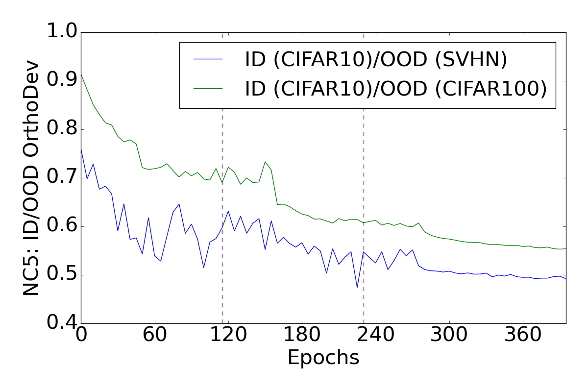
Figure 1: Convergence to ID/OOD orthogonality for ViT-B (left), Resnet-18 (right) both trained on CIFAR-10 as ID and tested in the presence of OOD data. Dashed purple lines indicate the end of warm-up steps in the case of ViT and learning rate decay epochs for ResNet-18.

4.1 NEural Collapse based Out of distribution detection (NECO) method

Based on this observation of orthogonality between ID and OOD samples, previous work (Wang et al., 2022; Cook et al., 2020) have utilised the null space for performing OOD detection. We now introduce notation and details these methods. Given an image ${\bm{x}}$ represented by feature vector $h_{\bm{\mathbf{\omega}}}(x)$, we impose that $f_{\bm{\mathbf{\omega}}}({\bm{x}})=W\times h_{\bm{\mathbf{\omega}}}({\bm{x}})$, where $W$ is the matrix of the last fully connected layer. Cook et al. (2020); Wang et al. (2022) have highlighted that features $h_{\bm{\mathbf{\omega}}}({\bm{x}})$ can be decomposed into two components: $h_{\bm{\mathbf{\omega}}}({\bm{x}})=h_{\bm{\mathbf{\omega}}}({\bm{x}})^{W}+h_{\bm{\mathbf{\omega}}}({\bm{x}})^{W^{\perp}}$. In this decomposition, $f_{\bm{\mathbf{\omega}}}({\bm{x}})=W\times h_{\bm{\mathbf{\omega}}}({\bm{x}})^{W}$, and importantly, $W\times h_{\bm{\mathbf{\omega}}}({\bm{x}})^{W^{\perp}}=0$. Hence, the component $h_{\bm{\mathbf{\omega}}}({\bm{x}})^{W^{\perp}}$ does not directly impact classification but plays a role in influencing OOD detection. In light of this observation, NuSA introduced the following score: $\mbox{NuSA}({\bm{x}})=\frac{\sqrt{\|h_{\bm{\mathbf{\omega}}}({\bm{x}})\|-\|h_{\bm{\mathbf{\omega}}}({\bm{x}})^{W^{\perp}}\|}}{\|h_{\bm{\mathbf{\omega}}}({\bm{x}})\|}$, and ViM introduced $\mbox{ViM}({\bm{x}})=\|h_{\bm{\mathbf{\omega}}}({\bm{x}})^{W^{\perp}}\|$. To identify the null space, NuSA optimizes the decomposition after training. On the other hand, ViM conducts PCA on the latent space $H$ (also after training), and decomposes it into a principal space, defined by the $d$-dimensional projection with the matrix $P\in M_{d,D}(\mathbb{R})$ spanned by the $d$ eigenvectors corresponding to the largest $d$ eigenvalues of the covariance matrix of $H$, and a null space, obtained by projecting on the remaining eigenvectors. In contrast, based on the implications of NC5, we propose a novel criterion that circumvents having to find the null space, specifically:

$$\mbox{NECO}({\bm{x}})=\frac{\|Ph_{\bm{\mathbf{\omega}}}({\bm{x}})\|}{\|h_{\bm{\mathbf{\omega}}}({\bm{x}})\|}=\frac{\sqrt{h_{\bm{\mathbf{\omega}}}({\bm{x}})^{\top}PP^{\top}h_{\bm{\mathbf{\omega}}}({\bm{x}})}}{\sqrt{h_{\bm{\mathbf{\omega}}}({\bm{x}})^{\top}h_{\bm{\mathbf{\omega}}}({\bm{x}})}}$$ (8)

Our hypothesis is that if the DNN is subject to the properties of NC1, NC2 and NC5, then it should be possible to separate any subset of ID classes from the OOD data. By projecting the feature into the first $d$ principal components extracted from the ID data, we should obtain a latent space representation that is close to the null vector for OOD data and not null for ID data. Consequently, by taking the norm of this projection and normalizing it with the norm of the data, we can derive an effective OOD detection criterion. However, in the case of vision transformers, the penultimate layer representation cannot straightforwardly be interpreted as features. Consequently, the resulting norm needs to be calibrated in order to serve as a proper OOD scoring function. To calibrate our NECO score, we multiply it by the penultimate layer biggest logit (MaxLogit). This has the effect of injecting class-based information into the score in addition to the desired scaling. It is worth noting that this scaling is also useful when the penultimate layer size is smaller than the number of classes, since in this case, it is not feasible to obtain maximum OrthoDev between all classes. We refer the reader to E for empirical observations on the distribution of NECO under the presence of OOD data.

4.2 Theoretical justification

To gain a better understanding of the impact of NECO, we visualize the Principal Component Analysis (PCA) of the pre-logit space in Figure 2, with ID data (colored points) and the OOD (black). This analysis is conducted on the ViT model trained on CIFAR-10, focusing on the first two principal components. Notably, the ID data points have multiple clusters, one by class, which can be attributed to the influence of NC1, and the OOD data points are positioned close to the null vector. To elucidate our criterion, we introduce an important property:

Theorem 4.1 (NC1+NC2+NC5 imply NECO).

We consider two datasets living in $\mathbb{R}^{D}$, $\{D_{\text{OOD}},D_{\tau}\}$ and a DNN $f_{\bm{\mathbf{\omega}}}(\cdot)=(g_{\bm{\mathbf{\omega}}}\circ h_{\bm{\mathbf{\omega}}})(\cdot)$ that satisfy NC1, NC2 and NC5. There $\exists\leavevmode\nobreak\ d\ll D$ for PCA on $D_{\tau}$ s.t. $\mbox{NECO}(\mu_{G}^{\mbox{OOD}})=0$. Conversely, for ${\bm{x}}\in D_{\tau}$ and considering ${\bm{x}}\neq\vec{0}$ we have that $\mbox{NECO}({\bm{x}})\neq 0$.

The proof for this theorem can be found in A

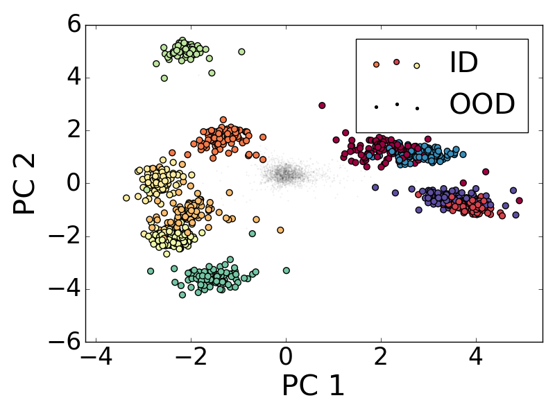
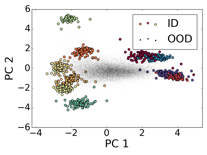
Figure 2: Feature projections on the first 2 principal components of a PCA fitted on CIFAR-10 (ID) using the ViT penultimate layer representation. OOD data are ImageNet-O (left), Textures (middle) and SVHN (right) . The Figure shows how NC1(1) property is satisfied by ID data, and that OOD data lie around the origin.

Remark 4.1.

We have established that $\mbox{NECO}(\mu_{G}^{\mbox{OOD}})=0$, which does not imply that $\mbox{NECO}({\bm{x}})=0$ for all ${\bm{x}}\in D_{\text{OOD}}$. However, in addition to NC5, we can put forth the hypothesis that NC2 is also occurring on the mix of ID/OOD data, while NC1 doesn’t occur on the OOD data by themselves. resulting in an OOD data cluster that is equiangular and orthogonal to the Simplex ETF structure. We refer the reader to Section D for justification. Furthermore, the observations made in Figure 2 appear to support our hypothesis.

5 Experiments & Results

In this section, we compare our method with state-of-the-art algorithms, on small-scale and large-scale OOD detection benchmarks. Following prior work, we consider ImageNet-1K, CIFAR-10 and CIFAR-100 as the ID datasets. We use both Transformer-based and CNN-based models to benchmark our method. Detailed experimental settings are as follows.

OOD Datasets.

For experiments involving ImageNet-1K as the inliers dataset (ID), we assess the model’s performance on five OOD benchmark datasets: Textures (Cimpoi et al., 2014), Places365 (Zhou et al., 2016), iNaturalist (Horn et al., 2017), a subset of 10 000 images sourced from (Huang & Li, 2021a), ImageNet-O (Hendrycks et al., 2021b) and SUN (Xiao et al., 2010). For experiments where CIFAR-10 (resp. CIFAR-100) serves as the ID dataset, we employ CIFAR-100 (resp. CIFAR-10) alongside the SVHN dataset (Netzer et al., 2011) as OOD datasets in these experiments. The standard dataset splits, featuring 50 000 training images and 10 000 test images, are used in these evaluations. Further details are provided in C.1. We refer the reader to E for additional testing results on the OpenOOD benchmark (Zhang et al., 2023).

Evaluation Metrics.

We present our results using two widely adopted OOD metrics (Yang et al., 2021). Firstly, we consider FPR95, the false positive rate when the true positive rate (TPR) reaches $95\%$, with smaller values indicating superior performance. Secondly, we use the AUROC metric, which is threshold-free and calculates the area under the receiver operating characteristic curve (TPR). A higher value here indicates better performance. Both metrics are reported as percentages.

Experiment Details.

We evaluate our method on a variety of neural network architectures, including Transformers and CNNs. ViT (Vision Transformer) (Dosovitskiy et al., 2020) is a Transformer-based image classification model which treats images as sequences of patches. We take the official pretrained weights on ImageNet-21K (Dosovitskiy et al., 2020) and fine-tune them on ImageNet-1K, CIFAR-10, and CIFAR-100. Swin (Liu et al., 2021) is also a transformer-based classification model. We use the officially released SwinV2-B/16 model, which is pre-trained on ImageNet-21K and fine-tuned on ImageNet-1K. From the realm of CNN-based models, we use ResNet-18 (He et al., 2015). When estimating the simplex ETF space, the entire training set is used. Further details pertaining to model training are provided in C.2. As a complementary experiment, we also assess our approach on DeiT Touvron et al. (2021) in E

Baseline Methods.

In our evaluation, we compared our method against twelve prominent post-hoc baseline approaches, which we list and provide ample details pertaining to implementation and associated hyper-parameters in B.

Model	Method	ImageNet-O AUROC$\uparrow$ FPR$\downarrow$	Textures AUROC$\uparrow$ FPR$\downarrow$	iNaturalist AUROC$\uparrow$ FPR$\downarrow$	SUN AUROC$\uparrow$ FPR$\downarrow$	Places365 AUROC$\uparrow$ FPR$\downarrow$	Average AUROC$\uparrow$ FPR$\downarrow$
ViT-B/16	Softmax score	85.31 52.65	86.64 49.40	97.21 12.14	86.64 53.75	85.52 56.93	88.26 44,97
	MaxLogit	92.23 36.40	91.69 36.90	98.87 5.72	92.15 39.88	90.05 46.75	92.99 33.13
	Energy	93.03 31.65	92.13 34.15	99.04 4.76	92.65 36.90	90.38 43.72	93.45 30.24
	Energy+ReAct	93.08 31.25	92.08 34.50	99.02 4.91	92.56 36.94	90.19 44.25	93.39 30.37
	ViM	94.01 28.95	91.63 38.22	99.59 2.00	92.73 34.00	89.67 44.12	93.56 29.46
	Residual	92.10 38.35	87.71 52.34	99.36 2.79	89.46 40.91	85.60 53.93	90.85 37.66
	GradNorm	84.70 34.85	86.29 35.76	97.45 6.17	86.67 39.49	83.59 46.94	87.74 32.64
	Mahalanobis	94.00 30.90	91.69 37.93	99.67 1.55	91.38 38.48	88.66 46.09	93.08 30.99
	KL-Matching	82.90 53.40	84.61 52.38	95.07 15.31	83.25 62.10	82.00 65.99	85.57 49.84
	ASH-B	69.28 85.25	66.05 83.29	72.62 80.62	59.36 91.53	55.08 92.68	64.48 86.67
	ASH-P	93.31 29.00	91.55 37.58	98.75 6.25	92.96 33.50	90.07 41.81	93.33 29.63
	ASH-S	92.85 29.45	91.00 39.73	98.50 7.28	92.61 33.12	89.55 41.68	92.90 30.25
	NECO (ours)	94.53 25.20	92.86 32.44	99.34 3.26	93.15 33.98	90.38 42.66	94.05 27.51
SwinV2	Softmax score	61.09 89.60	81.72 60.91	88.59 47.66	81.24 66.85	81.09 68.27	78.75 66.66
	MaxLogit	61.34 87.95	80.36 59.55	86.47 50.51	78.17 68.50	77.43 69.41	76.75 67.18
	Energy	61.32 85.75	77.91 64.44	81.85 63.44	73.80 76.89	73.09 76.68	73.59 73.44
	Energy+ReAct	68.38 83.85	84.56 59.86	90.23 51.97	82.61 69.27	81.41 70.19	81.44 67.03
	ViM	69.06 83.45	81.50 61.18	87.54 54.09	75.24 73.92	73.12 76.46	77.29 69.82
	Residual	66.82 83.80	77.36 65.00	83.23 59.77	71.03 76.41	68.90 78.53	73.47 72.70
	GradNorm	37.39 95.95	33.84 93.31	31.82 95.01	31.97 96.29	33.06 95.73	33.62 95.26
	Mahalanobis	71.87 86.05	84.51 63.35	89.81 57.10	80.28 75.39	78.52 77.10	80.99 71.80
	KL-Matching	58.60 87.50	75.30 71.69	82.93 58.29	73.72 76.53	72.11 78.91	72.53 74.58
	ASH-B	47.07 96.35	38.59 97.50	48.62 97.55	52.11 95.64	52.93 96.18	47.86 96.64
	ASH-P	37.38 97.95	26.51 98.90	20.73 99.28	24.49 99.08	26.12 98.93	27.05 98.83
	ASH-S	40.36 95.10	36.08 94.63	16.15 99.50	22.21 98.53	23.72 98.05	27.70 97.16
	NECO (ours)	65.03 80.55	82.27 54.67	91.89 34.41	82.13 62.26	81.46 64.08	80.56 59.19

Table 1: OOD detection for NECO and baseline methods. The ID dataset is ImageNet-1K, and OOD datasets are Textures, ImageNet-O, iNaturalist, SUN, and Places365. Both metrics AUROC and FPR95. are in percentage. A pre-trained ViT-B/16 model and SwinV2 are tested. The best method is emphasized in bold, and the 2nd and 3rd ones are underlined.

Result on ImageNet-1K.

In Table 1 we present the results for the ViT model in the first half. The best AUROC values are highlighted in bold, while the second and third best results are underlined. Our method demonstrates superior performance compared to the baseline methods. Across four datasets, we achieve the highest average AUROC and the lowest FPR95. Specifically, we attain a FPR95 of $27.51\%$, surpassing the second-place method, ViM, by $1.95\%$. The only dataset where we fall slightly behind is iNaturalist, with our AUROC being only $0.33\%$ lower than the best-performing approach. In Table 1, we provide the results for the SwinV2 model in the second half. Notably, our method consistently outperforms all other methods in terms of FPR95 on all datasets. On average, we achieve the third-best AUROC and significantly reduce the FPR95 by $7.47\%$ compared to the second-best performing method, Softmax score. We compare NECO with MaxLogit (Hendrycks et al., 2022) to illustrate the direct advantages of our scoring function. On average, we achieve a FPR95 reduction of $5.62\%$ for ViT and $7.99\%$ for Swin when transitioning from MaxLogit to NECO multiplied by the MaxLogit. This performance enhancement clearly underscores the value of incorporating the NC concept into the OOD detection framework. Moreover, NECO is straightforward to implement in practice, requiring simple post-hoc linear transformations and weight masking.

Results on CIFAR.

Table 2 presents the results for the ViT model and Resnet-18 both on CIFAR-10 and CIFAR-100 as ID dataset, tested against different OOD datasets. On the first half of the table, we show the results using a ViT model. On the majority of the OOD datasets cases we outperform the baselines both in terms of FPR95 and AUROC. Only ASH outperform NECO on the use case CIFAR-100 vs SVHN. On average we surpass all the baseline on both test sets. On second half, we show the results using a ResNet-18 model. Similarly to ViT results, on average we surpass the baseline strategies by at least 1.28% for the AUROC on the CIFAR-10 cases and lowering the best baseline performance by 8.67% in terms of FPR95, on the CIFAR-100 cases. On average, our approach outperforms baseline methods in terms of AUROC. However, we notice that our method performs slightly worse on the CIFAR-100-ID/CIFAR-10-OOD task.

		CIFAR-100 AUROC$\uparrow$ FPR$\downarrow$	SVHN AUROC$\uparrow$ FPR$\downarrow$	Average AUROC$\uparrow$ FPR$\downarrow$	CIFAR-10 AUROC$\uparrow$ FPR$\downarrow$	SVHN AUROC$\uparrow$ FPR$\downarrow$	Average AUROC$\uparrow$ FPR$\downarrow$
ViT	Softmax score	98.36 7.40	99.64 0.59	99.00 3.99	92.13 34.74	91.29 39.56	91.71 37.15
	MaxLogit	98.60 5.94	99.90 0.23	99.25 3.09	92.81 26.73	96.20 18.68	94.51 22.71
	Energy	98.63 5.93	99.92 0.21	99.28 3.07	92.68 26.37	96.68 15.72	94.68 21.05
	Energy+ReAct	98.68 5.92	99.92 0.23	99.30 3.08	93.43 25.93	96.65 15.88	95.04 20.91
	ViM	98.81 4.86	99.50 0.82	99.16 2.84	94.78 26.10	95.55 26.33	95.17 26.22
	Residual	98.49 7.09	96.95 12.64	97.72 9.87	94.63 28.42	92.43 44.65	93.53 36.54
	GradNorm	95.82 10.92	99.85 0.48	97.84 5.7	92.10 26.20	94.85 16.69	93.48 21.45
	Mahalanobis	98.73 5.95	95.52 18.61	97.13 12.28	95.42 24.02	93.91 37.11	94.67 30.57
	KL-Matching	83.48 20.65	95.07 6.09	89.28 13.37	79.47 38.34	80.19 41.73	79.83 40.04
	ASH-B	95.15 17.49	99.09 4.81	97.12 11.15	78.07 53.01	82.99 53.97	80.53 53.49
	ASH-P	97.89 7.22	99.90 0.26	98.90 3.74	85.12 29.82	97.04 14.06	91.08 21.94
	ASH-S	97.56 7.73	99.89 0.32	98.73 4.03	83.30 30.96	97.04 14.55	90.17 22.56
	NECO (ours)	98.95 4.81	99.93 0.12	99.44 2.47	95.17 23.39	96.65 15.47	95.41 19.43
ResNet-18	Softmax score	85.07 67.41	92.14 46.77	88.61 57.09	75.35 83.09	77.30 85.61	76.33 84.35
	MaxLogit	85.36 59.19	93.73 31.52	89.55 45.36	75.44 83.12	77.24 87.59	76.34 85.36
	Energy	85.46 58.68	93.96 29.71	89.71 44.20	75.25 83.76	76.40 90.77	75.83 87.27
	Energy+ReAct	84.22 60.04	92.31 35.17	88.27 47.61	70.00 85.99	74.14 91.05	72.07 88.52
	ViM	85.11 63.76	94.87 27.35	89.99 45.56	67.61 90.08	86.13 67.31	76.87 78.70
	Residual	76.06 76.53	90.21 48.18	83.14 62.36	45.99 96.19	72.52 86.60	59.23 91.40
	GradNorm	60.83 69.98	78.28 42.83	69.56 56.41	72.62 84.64	69.66 91.58	59.55 88.11
	Mahalanobis	81.23 72.35	90.39 54.51	85.81 63.43	55.85 95.41	79.96 81.63	67.91 88.52
	KL-Matching	77.83 68.12	86.73 49.47	82.28 58.80	73.52 83.05	77.32 74.82	67.91 78.94
	ASH-B	73.89 64.45	83.79 44.77	78.84 54.61	74.10 84.00	78.14 82.02	76.12 83.01
	ASH-P	83.96 59.90	94.77 26.04	89.37 42.97	75.46 82.98	77.28 89.43	:76.37 86.21
	ASH-S	82.48 62.38	91.54 39.94	87.01 51.16	72.17 85.20	80.18 74.39	76.18 80.00
	NECO (ours)	86.61 57.81	95.92 20.43	91.27 39.12	70.26 85.70	88.57 54.35	79.42 70.03

Table 2: OOD detection for NECO vs baseline methods. The ID dataset are CIFAR-10/CIFAR-100, and OOD datasets are CIFAR-100/CIFAR-10 alongside SVHN. Both metrics AUROC and FPR95 are in percentage. The best method is emphasized in bold, and the 2nd and 3rd ones are underlined.

6 Conclusion

This paper introduces an novel OOD detection method that capitalizes on the Neural Collapse (NC) properties inherent in DNNs. Our empirical findings demonstrate that when combined with over-parameterized DNNs, our post-hoc approach, NECO, achieves state-of-the-art OOD detection results, surpassing the performance of most recent methods on standard OOD benchmark datasets. While many existing approaches focus on modelling the noise by either clipping it or considering its norm, NECO takes a different approach by leveraging the prevalent ID information in the DNN, which will only be enhanced with model improvements. The latent space contains valuable information for identifying outliers, and NECO incorporates an orthogonal decomposition method that preserves the equiangularity properties associated with NC.
We have introduced a novel NC property (NC5) that characterizes both ID and OOD data behaviour. Through our experiments, we have shed light on the substantial impact of NC on the OOD detection abilities of DNNs, especially when dealing with over-parameterized models. We observed that NC properties, including NC5, NC1, and NC2, tend to converge towards zero as expected when the network exhibits over-parameterization. This empirical observation provides insights into why our approach performs exceptionally on a variety of models and on a broad range of OOD dataset (we refer the reader to the complementary results in E), hence demonstrating the robustness of NECO against OOD data.

While our approach excels with Transformers and CNNs, especially in the case of over-parametrized models, we observed certain limitations when applying it to DeiT (see the results in E). These limitations may be attributed to the distinctive training process of DeiT (i.e., including a distillation strategy) which necessitates a specific setup that we did not account for in order to prevent introducing bias to the NC phenomenon. We hope that this work has shed some light on the interactions between NC and OOD detection. Finally, based on our results and observations, this work raises new research questions on the training strategy of DNNs that lead to NC in favor of OOD detection.

1

Table of Contents - Supplementary Material

Appendix A Theoretical justification

Before proceeding with the proof of Theorem 4.1, we first introduce some notation and a useful lemma for the subsequent proof.

Given a vector ${\bm{z}}_{1}\in\mathbb{R}^{D}$ we define ${\bm{z}}_{1}^{PCA}$ as the projection of ${\bm{z}}_{1}$ onto a subspace obtained by applying PCA to an external dataset $D$ of same dimensionality as ${\bm{z}}_{1}$. This subspace has dimensions limited to $d\leq D$.

Lemma A.1 (Orthogonality conservation).

We consider a single dataset, $D_{1}=\{{\bm{h}}_{i}\}_{i=1}^{n}\in\mathbb{R}^{D}$, along with two vectors, $\{{\bm{z}}_{1},{\bm{z}}_{2}\}\in\mathbb{R}^{D}$, that are not necessarily part of $D_{1}$ with the condition that $\langle{\bm{z}}_{1},{\bm{z}}_{2}\rangle=0$. Considering a PCA on $D_{1}$, it follows that $\langle{\bm{z}}_{1}^{PCA},{\bm{z}}_{2}^{PCA}\rangle=0$.

Proof.

If ${\bm{z}}_{1}\perp{\bm{z}}_{2}$, then we have ${\bm{z}}_{1}^{\top}{\bm{z}}_{2}=0$. Let us define $P\in\mathbb{M}_{D,d}(\mathbb{R})$ the projection matrix of the $PCA$.
By definition $P$ is an orthogonal matrix, hence $P^{\top}P=I_{d}$ and $PP^{\top}=I_{D}$, where $I_{D}$ and $I_{d}$ are the identity matrices of $\mathbb{M}_{D\times D}(\mathbb{R})$ and $\mathbb{M}_{d\times d}(\mathbb{R})$, respectively. We have $({\bm{z}}_{1}^{PCA})^{\top}{\bm{z}}_{2}^{PCA}=(P^{\top}{\bm{z}}_{1})^{\top}(P^{\top}{\bm{z}}_{2})={\bm{z}}_{1}^{\top}PP^{\top}{\bm{z}}_{2}={\bm{z}}_{1}^{\top}I_{D}{\bm{z}}_{2}={\bm{z}}_{1}^{\top}{\bm{z}}_{2}=0,\text{ thus proving the orthogonality of PCA projections.}$ ∎

This lemma asserts that the PCA projection keeps the orthogonal property of two vectors, which will be of great importance towards the proof of the next theorem.

For completeness, we reiterate the theorem, followed by the proof.

Theorem A.2 (NC1+NC2+NC5 imply NECO).

We consider two datasets living in $\mathbb{R}^{D}$, $\{D_{\text{OOD}},D_{\tau}\}$ and a DNN $f_{\bm{\mathbf{\omega}}}(\cdot)=(g_{\bm{\mathbf{\omega}}}\circ h_{\bm{\mathbf{\omega}}})(\cdot)$ that satisfy NC1, NC2 and NC5. There $\exists\leavevmode\nobreak\ d\ll D$ for PCA on $D_{\tau}$ s.t. $\mbox{NECO}(\mu_{G}^{\mbox{OOD}})=0$. Conversely, for ${\bm{x}}\in D_{\tau}$ and considering ${\bm{x}}\neq\vec{0}$ we have that $\mbox{NECO}({\bm{x}})\neq 0$.

Proof.

Assuming, for the sake of contradiction, that we have $\forall d\leq D$ s.t. $\mbox{NECO}(\mu_{G}^{\mbox{OOD}})\neq 0$ and $\mbox{NECO}({\bm{x}})=0$ for data points ${\bm{x}}$ in $D_{\tau}$. Given a PCA dimension $d$ s.t. $d\geq C$ and based on the mathematical underpinnings of PCA, most data points ${\bm{x}}$ in $D_{\tau}$ satisfy the condition that $\|Ph_{\bm{\mathbf{\omega}}}({\bm{x}})\|$ is maximized and therefore not equal to zero.
Considering our assumption of NC2 + NC1, we can infer that each class $c$ resides within a one-dimensional space that is aligned with $\mu_{c}$. As a result, the set of vectors $\{\mu_{c}\}_{c=1}^{C}$ forms an orthogonal basis. According to the PCA definition, the dimensional space resulting from PCA, when $d=C$, should be spanned by the set $\{\mu_{c}^{\mbox{PCA}}\}_{c=1}^{C}$. Here, for each class $c$, $\mu_{c}^{\mbox{PCA}}$ represents the PCA projection of $\mu_{c}$.
Utilizing the orthogonality conservation lemma and considering our assumption of NC5, we can deduce that each $\mu_{c}^{\mbox{PCA}}$ is orthogonal to $\mu_{G}^{\mbox{OOD}}$. Consequently, we can confidently state that $\mbox{NECO}(\mu_{G}^{\mbox{OOD}})=0$, thereby achieving the sought contradiction. ∎

Appendix B Details on Baselines Implementations

In this section, we provide an overview of the various baseline methods utilized in our experiments. We explain the mechanisms underlying these baselines, detail the hyperparameters employed, and offer insights into the process of determining hyperparameters when a baseline was not originally designed for a specific architecture.

ASH.

ASH, as introduced by Djurisic et al. (2022), employs activation pruning at the penultimate layer, just before the application of the DNN classifier. This pruning threshold is determined on a per-sample basis, eliminating the need for pre-computation of ID data statistics. The original paper presents three different post-hoc scoring functions, with the only distinction among them being the imputation method applied after pruning. In ASH-P, the clipped values are replaced with zeros. ASH-B substitutes them with a constant equal to the sum of the feature vector before pruning, divided by the number of kept features. ASH-S imputes the pruned values by taking the exponential of the division between the sum of the feature vector before pruning and the feature vector after pruning. Since our study employs different models than the original ASH paper by Djurisic et al. (2022), we fine-tuned their method using a range of threshold values, specifically $[65,70,75,80,85,90,95,99]$, for their three variations of ASH, consistent with the thresholds used in the original paper. The optimized ASH thresholds are presented in Table B.3.

Ash Variant		CIFAR-10	CIFAR-100	ImageNet
ASH-B	ViT	75	60	70
	SwinV2-B/16	-	-	99
	DeiT-B/16	-	-	60
	ResNet-18	75	90	-
ASH-P	ViT	60	60	60
	SwinV2-B/16	-	-	60
	DeiT-B/16	-	-	60
	ResNet-18	95	85	-
ASH-S	ViT	60	60	60
	SwinV2-B/16	-	-	99
	DeiT-B/16	-	-	99
	ResNet-18	60	85	-

Table B.3: Ash optimised pruning threshold per-model and per-dataset. Values are in percentage.

ReAct.

For the ReAct baseline, we adopt the ReAct+Energy setting, which has been identified as the most effective configuration in prior work Sun et al. (2021). The original paper determined that the 90th percentile of activations estimated from the in-distribution (ID) data was the optimal threshold for clipping. However, given that we employed different models in our experiments, we found that using a rectification percentile of $p=99$ yielded better results in terms of reducing the false positive rate (FPR95) for models like ViT and DeiT, while a percentile of $p=0.95$ was more suitable for Swin. In our reported results, we use the best threshold setting for each model accordingly to ensure optimal performance.

ViM and Residual.

Introduced by Wang et al. (2022), ViM decomposes the latent space into a principal space $P$ and a null space $P^{\perp}$. The ViM score is then computed by using the projection of the features on the null space to create a virtual logit, using the norm of this projection along with the logits. In addition, they calibrate the obtained norm by a constant alpha to enhance their performance. Alpha is the division of the sum of the Maximum logits, divided by the sum of the norms in the null space projection, both measured on the training set.
As for Residual, the score is obtained by computing the norm of the latent vector projection in the null space.
We followed ViM official paper (Wang et al., 2022) recommendation for the null space dimenssion in the ViT, DeiT and swin, i.e., [512,512,1000] respectively. However, the case of ResNet-18 was not considered in the paper. We found that a 300 latent space dimension works best in reducing the FPR.

Mahalanobis.

We have also implemented the Mahalanobis score by utilizing the feature vector before the final classification layer, which corresponds to the DNN classifier, following the methodology outlined in Fort et al. (2021). To estimate the precision matrix and the class-wise average vector, we utilize the complete training dataset. It is important to note that we incorporate the ground-truth labels during the computation process.

KL-Matching.

We calculate the class-wise average probability by considering the entire training dataset. In line with the approach described in Hendrycks et al. (2022), we rely on the predicted class rather than the ground-truth labels for this calculation.

Softmax score.

Hendrycks & Gimpel (2017) uses the maximum softmax probability (MSP) of the model as an OOD scoring function.

MaxLogit.

Hendrycks et al. (2022) uses the maximum logit value (Maxlogit) of the model as an OOD scoring function.

GradNorm.

Huang & Li (2021a) computes the norm of gradients between the softmax output and a uniform probability distribution.

Energy.

Liu et al. (2020) proposes to use the energy score for OOD detection. The energy function maps the logit outputs to a scalar $Energy(x;f)\in\mathbb{R}$. In order to keep the convention that the score need to be lower for ID data, Liu et al. (2020) used the negative energy as the OOD score.

Appendix C Additional Experiment Details

C.1 OOD datasets

For experiments involving ImageNet-1K as the inliers dataset (ID), we assess the model’s performance on five OOD benchmark datasets. Textures (Cimpoi et al., 2014) dataset comprises natural textural images, with the exclusion of four categories (bubbly, honeycombed, cobwebbed, spiralled) that overlap with the inliers dataset. Places365 (Zhou et al., 2016) is a dataset consisting of images depicting various scenes. iNaturalist (Horn et al., 2017) dataset focuses on fine-grained species classification. We utilize a subset of 10 000 images sourced from (Huang & Li, 2021a). ImageNet-O (Hendrycks et al., 2021b) is a dataset comprising adversarially filtered images designed to challenge OOD detectors. SUN (Xiao et al., 2010) is a dataset containing images representing different scene categories. Figure C.3 shows five examples from each of these datasets.
For experiments where CIFAR-10 (resp. CIFAR-100) serves as the ID dataset, we employ CIFAR-100 (resp. CIFAR-10) as OOD dataset. Additionally, we include the SVHN dataset (Netzer et al., 2011) as OOD datasets in these experiments. The standard dataset splits, featuring 50 000 training images and 10 000 test images, are used in these evaluations.

Figure C.3: Example images from ImageNet-1k considered OOD datasets. Each row representing an OOD dataset: ImageNet-O, Textures, iNaturalist, SUN and Places365 respectively from top to bottom.

C.2 Fine-tuning details

The fine-tuning setup for the ViT model is as follows: we take the official pretrained weights on ImageNet-21K (Dosovitskiy et al., 2020) and fine-tune them on ImageNet-1K, CIFAR-10, and CIFAR-100. For ImageNet-1K, the weights are fine-tuned for 18 000 steps, with 500 cosine warm-up steps, 256 batch size, 0.9 momentum, and an initial learning rate of $2\mathrm{x}10^{-2}$. For CIFAR-10 and CIFAR-100 the weights are fine-tuned for 500 and 1000 steps respectively. With 100 warm-up steps, 512 batch size and the rest of training parameters being equal to the case of ImageNet-1K. Swin (Liu et al., 2021) is also a transformer-based classification model. We use the officially released SwinV2-B16 model, which is pre-trained on ImageNet-21K and fine-tuned on ImageNet-1K. ResNet-18 (He et al., 2015) is a CNN-based model. For both CIFAR-10 and CIFAR-100, the model is trained for 200 epochs with 128 batch size, $5\mathrm{x}10^{-4}$ weight decay and 0.9 momentum. The initial learning rate is 0.1 with a cosine annealing scheduler. When estimating the simplex ETF space, the entire training set is used.

C.3 Dimension of Equiangular Tight Frame (ETF)

In Figures C.5,C.6 and C.4, we shows the performances, in terms of AUROC and FPR95, for different models, with different ID data: ImageNet, CIFAR-10 or CIFAR-100. We observe that both performance metrics remain

relatively stable once the dimension rises over a certain threshold for each case study. This suggests that including more dimensions beyond this threshold adds little to no meaningful information about the ID data. We hypothesize that the inflection point in these curves indicates the best approximate subspace dimension of the Simplex ETF relevant to our ID data. Therefore, for greater adaptability, Table C.4 shows the best ETF values that minimize the FPR (and maximize the AUC in case of equal FPR) for each tuple dataset. Hence, our results depicted in Section 5 utilize the best ETF values for each tuple <model, ID, OOD>. In more general case, according to Figures C.5,C.6 and C.4, we still have the flexibility to find a single ETF dimension per ID dataset and model if the specific application demands it while maintaining state-of-the-art performance.

ID Data	Model	ImageNet-O	Textures	iNaturalist	SUN	Places365	CIFAR-10	CIFAR-100	SVHN
ImageNet	ViT-B/16	140	270	490	270	360	-	-	-
	SwinV2-B/16	70	510	450	560	670	-	-	-
	DeiT-B/16	430	670	370	710	730	-	-	-
CIFAR-10	ViT-B/16	-	-	-	-	-	-	40	100
	ResNet-18	-	-	-	-	-	-	130	250
CIFAR-100	ViT-B/16	-	-	-	-	-	130	-	260
	ResNet-18	-	-	-	-	-	150	-	470

Table C.4: Best Simplex ETF approximate dimension, for different DNN architectures and ID data case studies: ImageNet, CIFAR-10 and CIFAR-100. The Best ETF dimension is found by minimizing the FPR95, then maximizing the AUROC in case of equal FPR95 accross the dimensions. The values are presented for different DNN architectures and ID data (ImageNet, CIFAR-10 and CIFAR-100) and their respective OOD test cases.

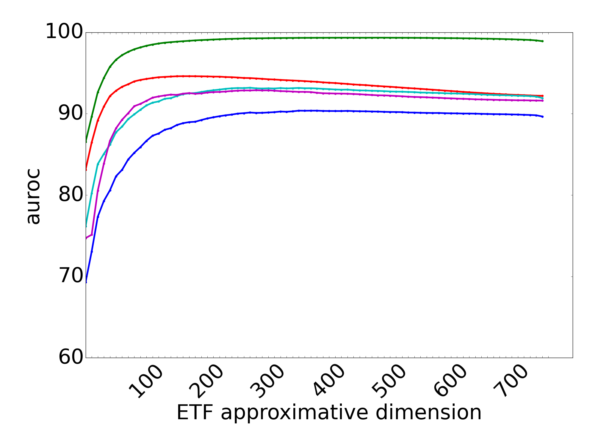
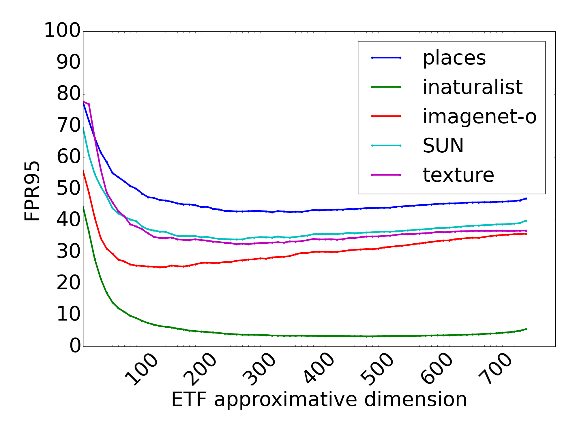
(a) ViT Model

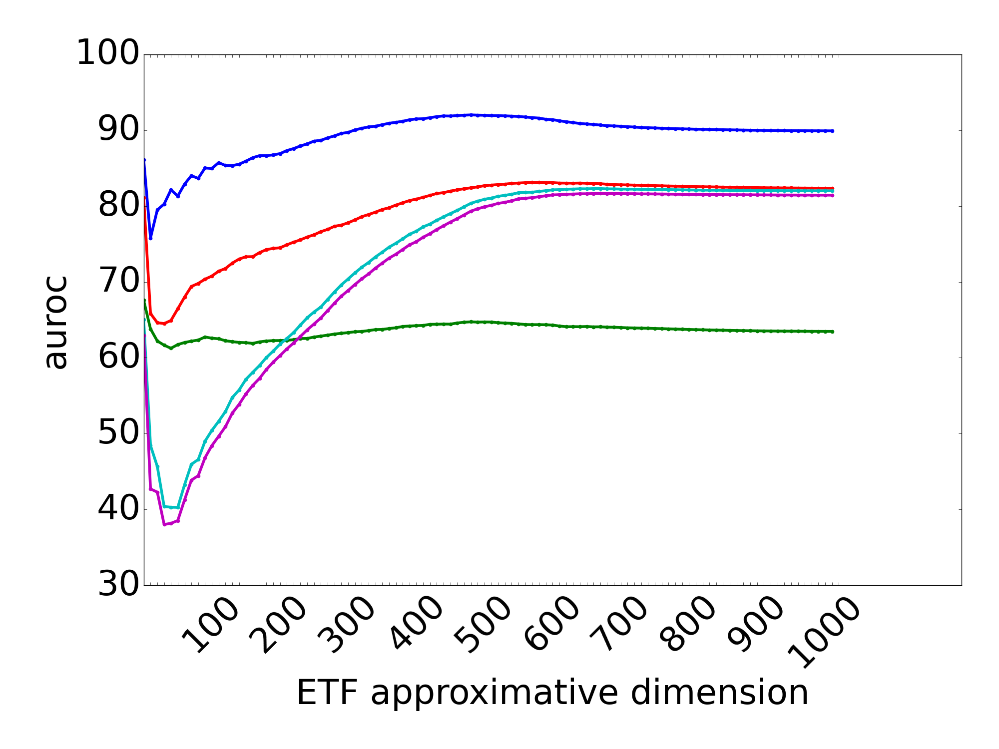
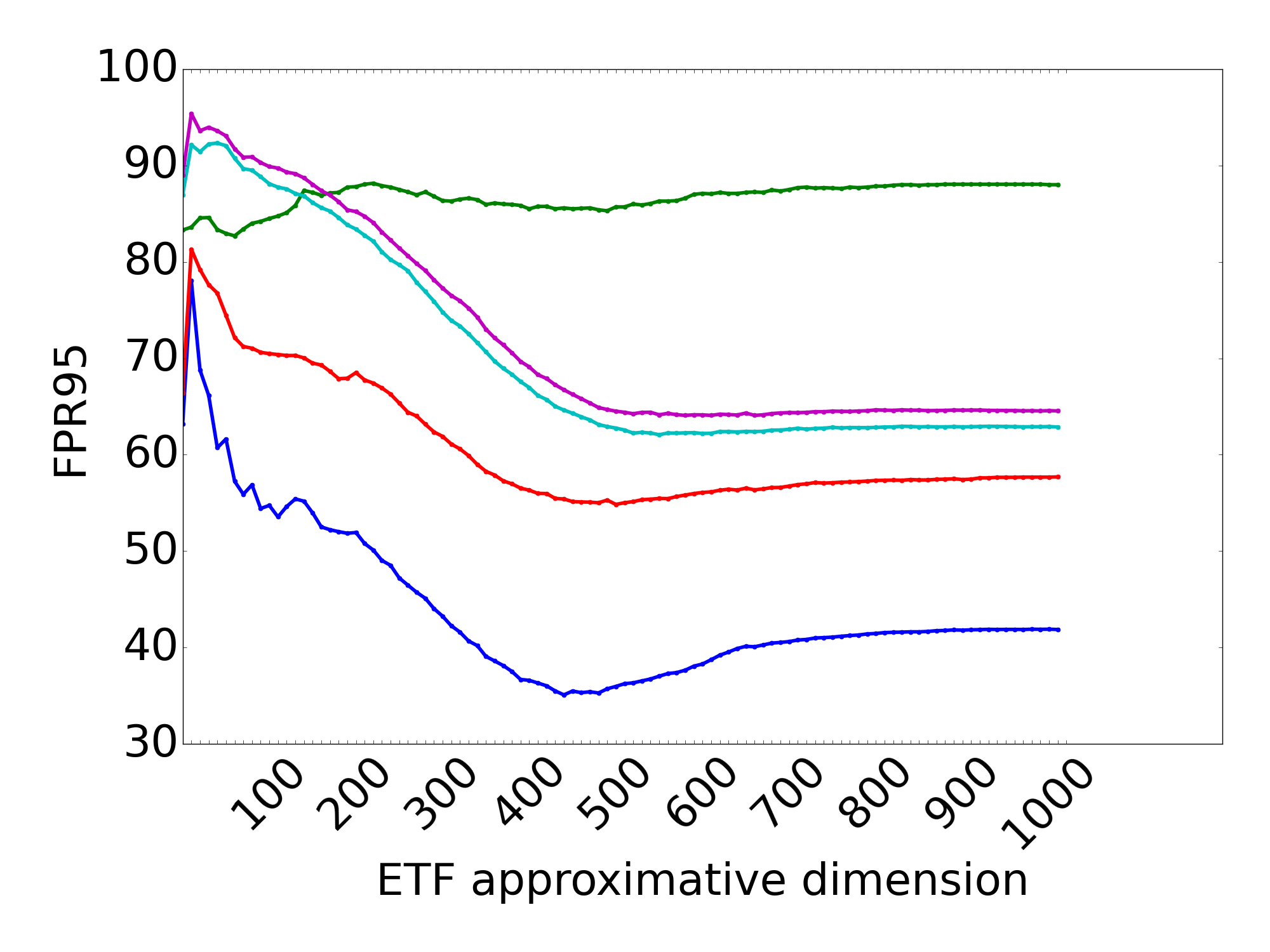
(b) SwinV2 Model

Figure C.4: Comparison of Performance metrics — AUROC (left) and FPR95 (right) — against the principal space dimension, for ViT (Top) and SwinV2 (Bottom), with ImageNet as ID data and different OOD datasets: iNaturalist, ImageNet-O, Textures, SUN, Places365.

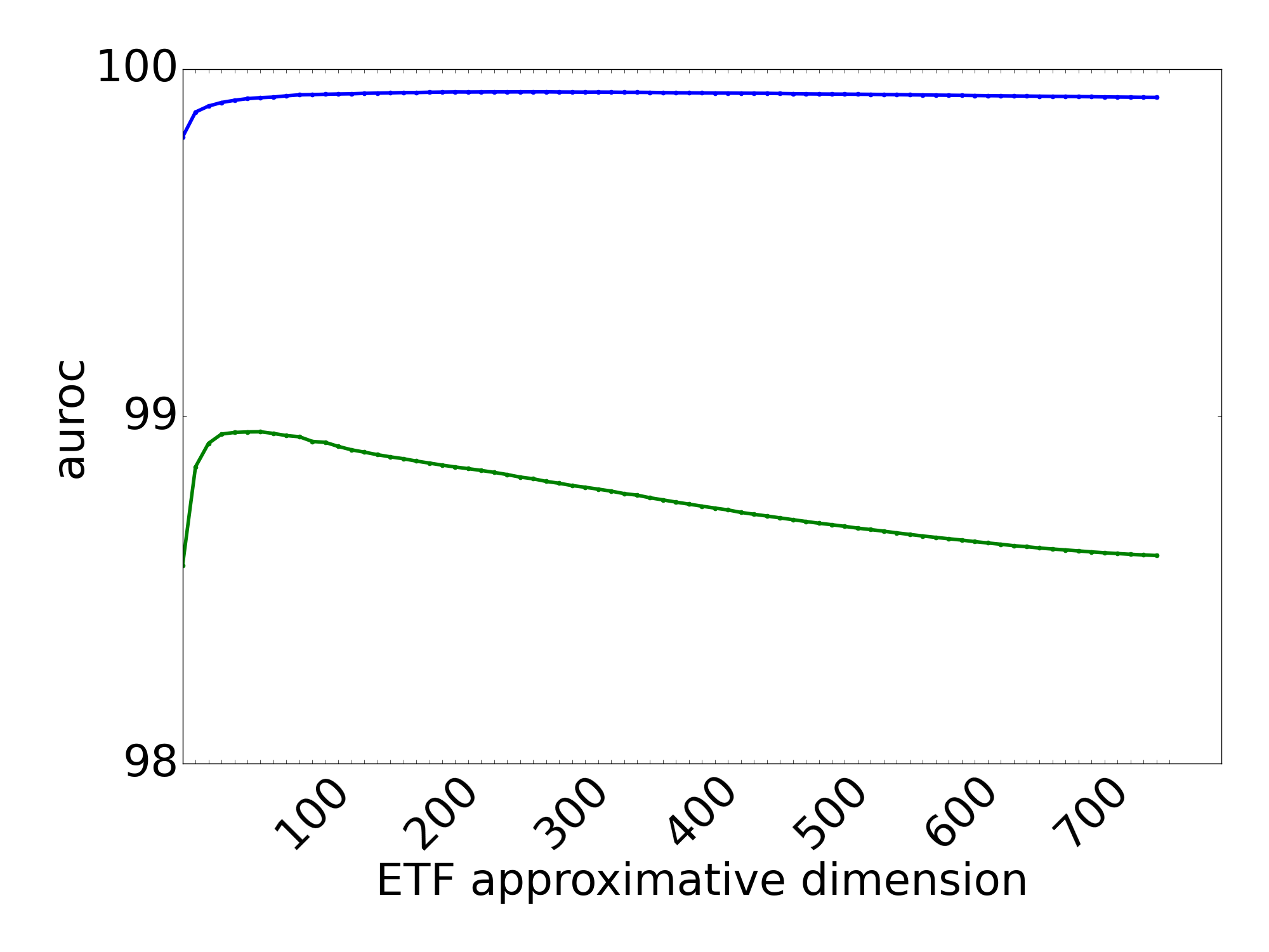
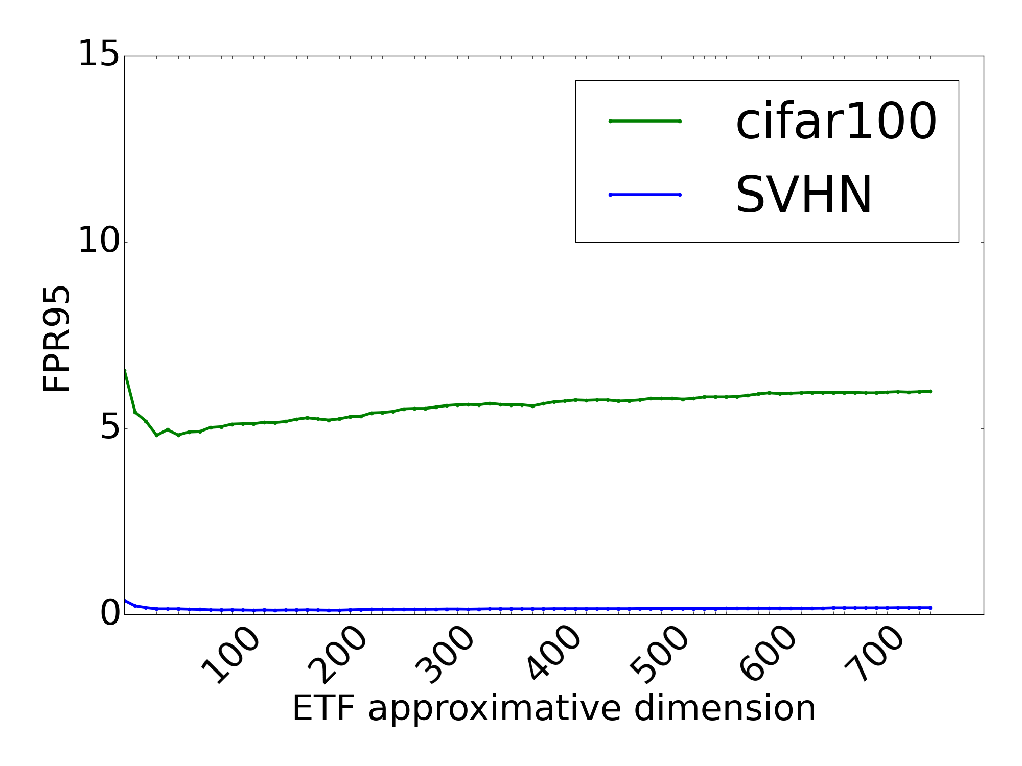
(a) ViT Model

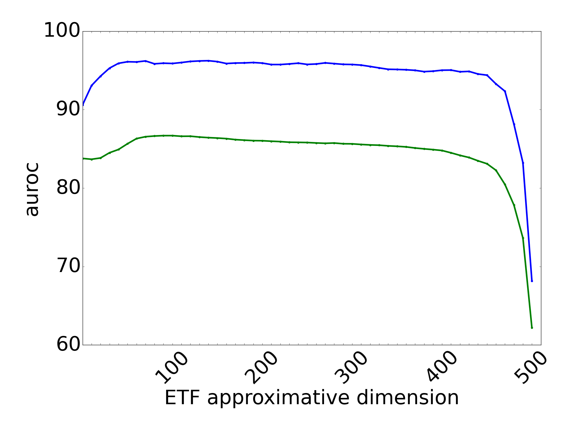
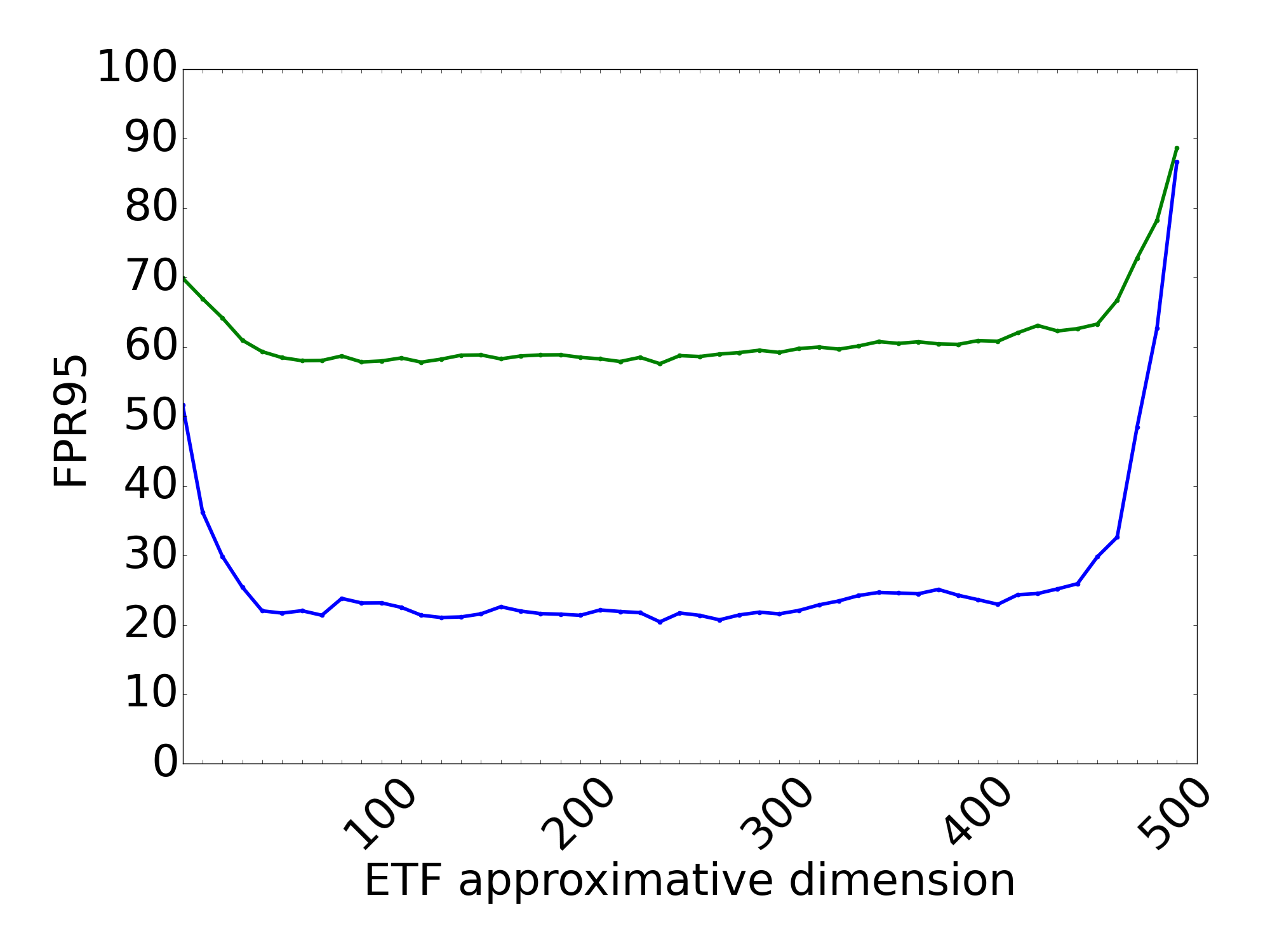
(b) ResNet-18 Model

Figure C.5: Comparison of Performance metrics — AUROC (left) and FPR95 (right) — against the principal space dimension, for ViT (Top) and ResNet-18 (Bottom), with CIFAR-10 as ID data, and different OOD datasets: SVHN, CIFAR-100.

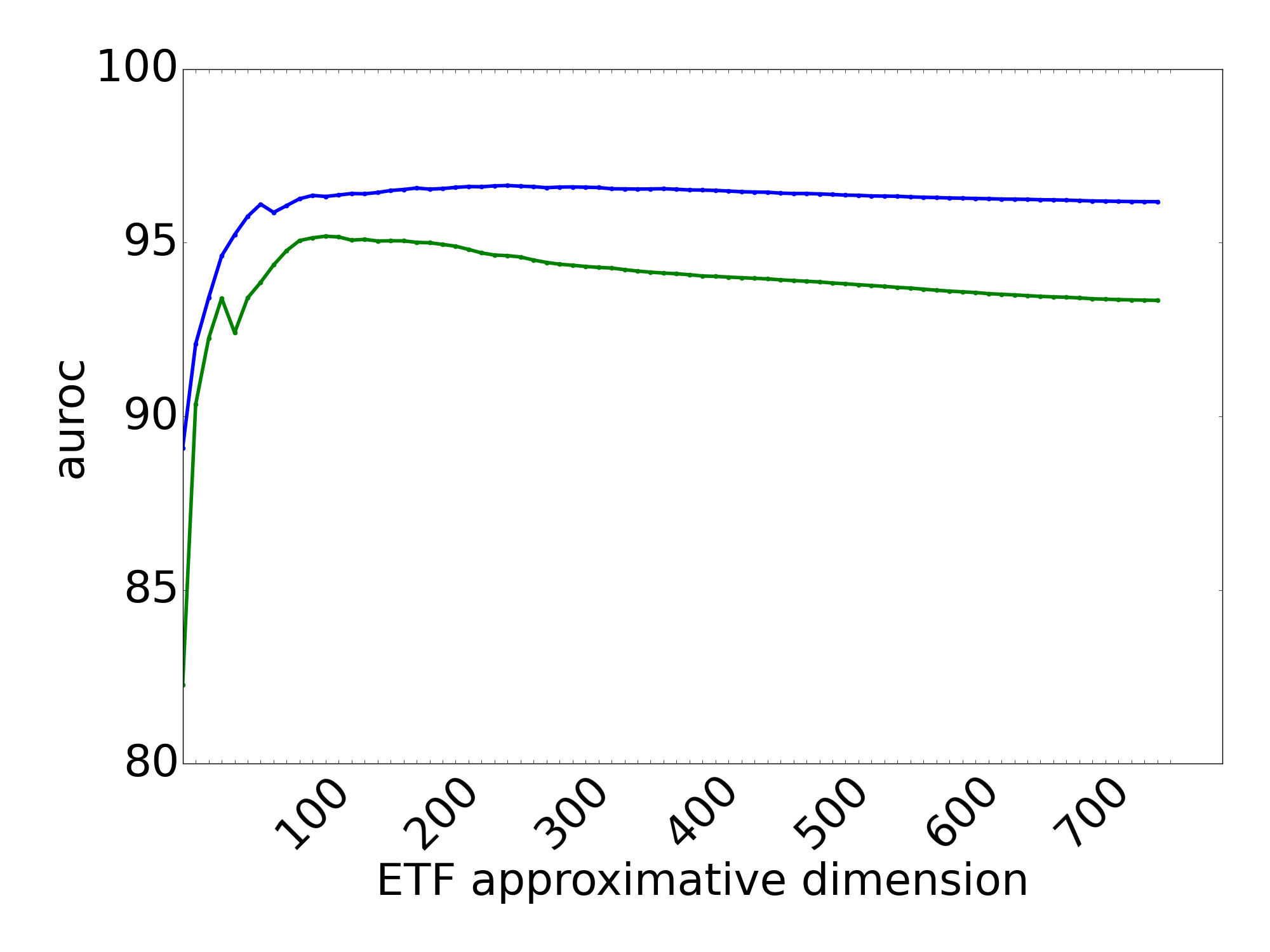
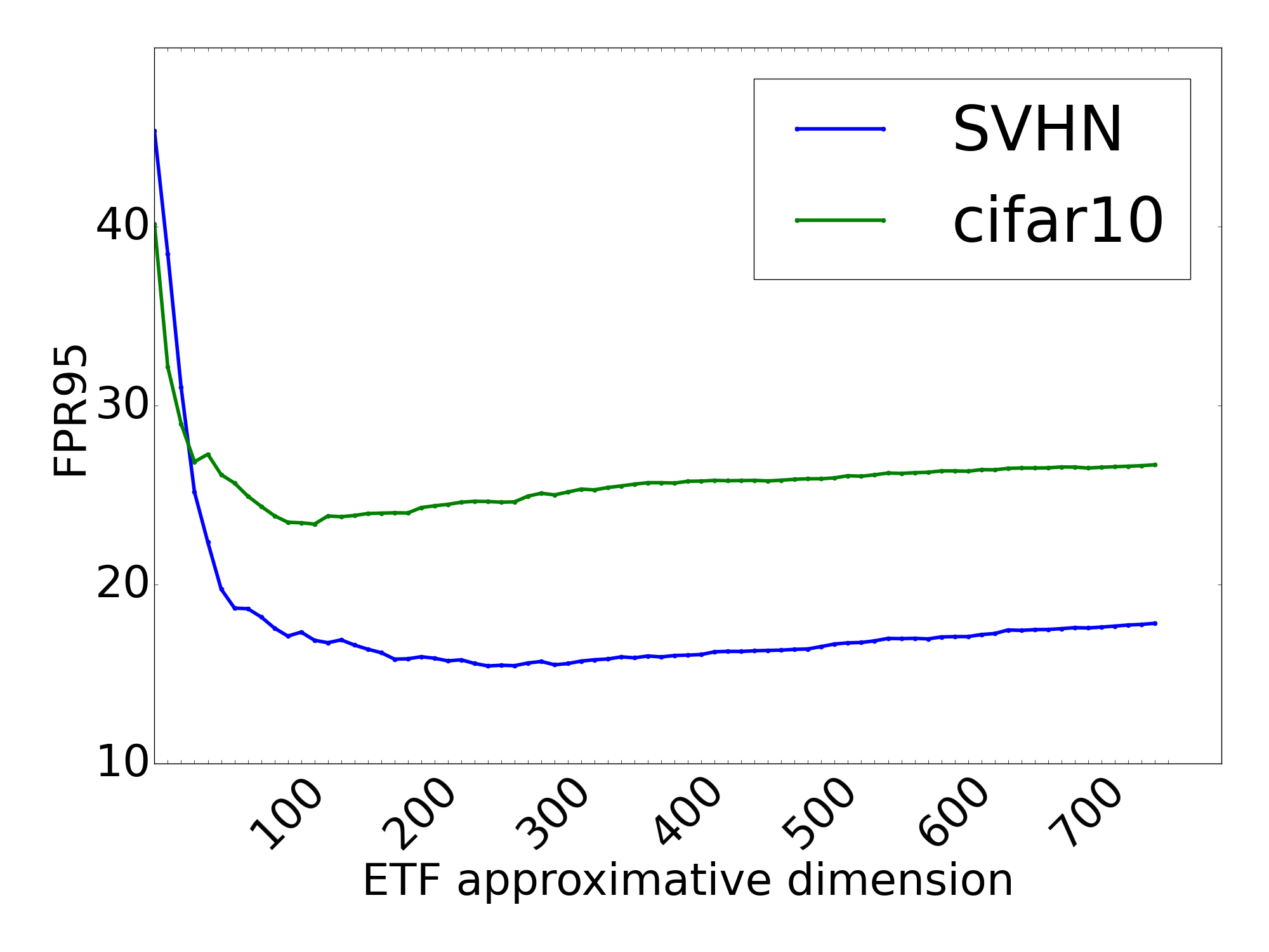
(a) ViT Model

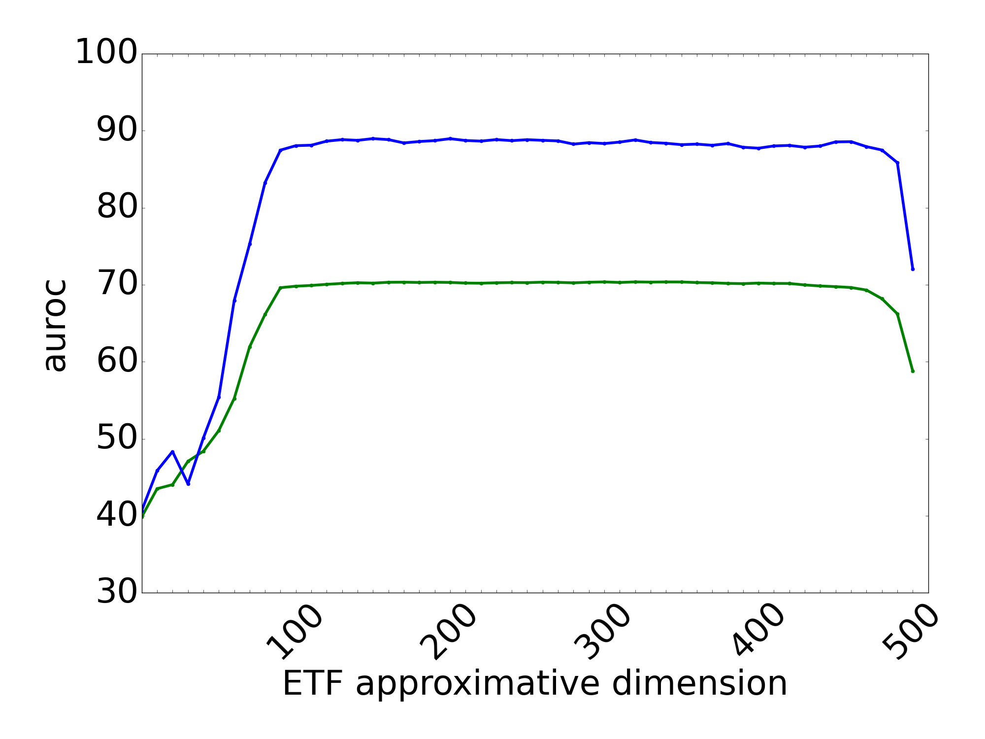
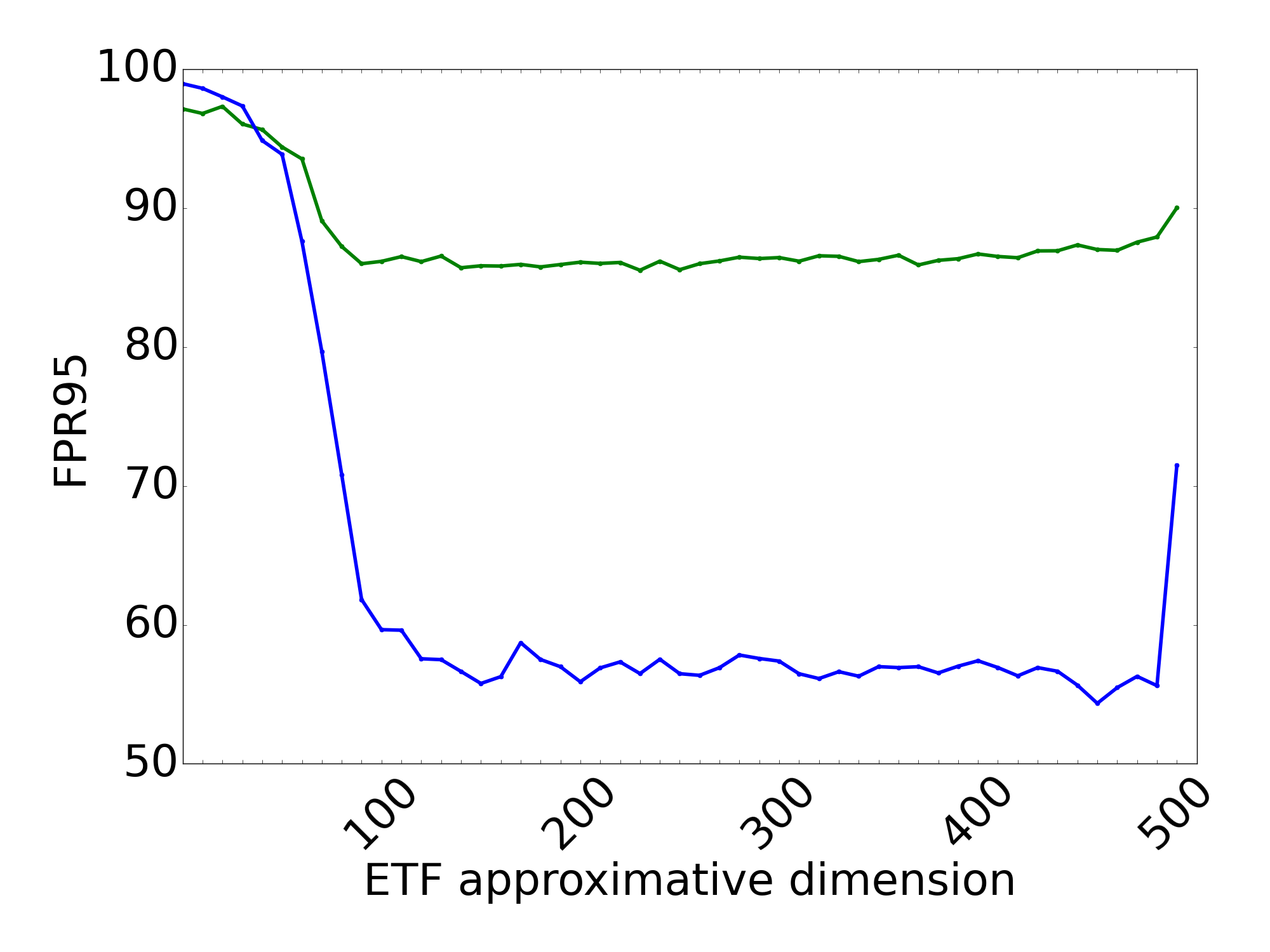
(b) ResNet-18 Model

Figure C.6: Comparison of Performance metrics — AUROC (left) and FPR95 (right) — against the principal space dimension, for ViT (Top) and ResNet-18 (Bottom), with CIFAR-100 as ID data, and different OOD datasets: SVHN, CIFAR-10.

C.4 Classification Accuracy

Considering the post hoc nature of our method, when an input image is identified as in-distribution (ID), it is important to note that one can always use the original DNN classifier. This switch comes with a negligible overhead and ensures optimal performance for both classification and out-of-distribution (OOD) detection. Consequently, the classification performance of the final model remains unaltered in our approach. We refer the reader to Table C.5 for the observed classification accuracy.

ID Data	Model	Architecture	Pre-trained dataset	Accuracy (top1%)
ImageNet	ViT-B/16	Transformer	ImageNet-21k	83.84
	SwinV2-B/16	Transformer	ImageNet-21k	81.20
	DeiT-B/16	Transformer	ImageNet-21k	81.80
CIFAR-10	ViT-B/16	Transformer	ImageNet-21k	98.89
	ResNet-18	Residual Convnet	-	95.46
CIFAR-100	ViT-B/16	Transformer	ImageNet-21k	92.16
	ResNet-18	Residual Convnet	-	78.59

Table C.5: Top 1% accuracy on ID data for the original classification task, for the models and ID dataset considered in our experiments, including relevant model details (from the type of architecture to with/without pretraining distinction).

Appendix D Details about Neural Collapse

D.1 Additional neural collapse properties

Here, we present the equations for the remaining two properties of “neural collapse”. We evaluate the convergence to Self-duality (NC3) using the following expression:

$$\operatorname{Self-duality}=\|\tilde{W}^{\top}-\tilde{M}\|^{2}_{2}\leavevmode\nobreak\ ,$$ (9)

In this equation, $W$ represents the matrix of the penultimate layer classifier weights, $M$ is the matrix of class means, and $[\tilde{\cdot}]$ denotes a matrix with unit-normalized means over columns. Additionally, $\|\cdot\|^{2}_{2}$ signifies the square of the $L2$ norm.

Moreover, the Simplification to Nearest Class-Center (NC4, see Equation 4) is measured as the proportion of training set samples that are misclassified when we apply the simple decision rule of assigning each feature space activation to the nearest class mean:

$$\operatorname{Simplification-to-NCC}=\operatorname{argmin}_{c}\|z-\mu_{c}\|_{2}\leavevmode\nobreak\ ,$$ (10)

where $z$ represents the feature vector for a given input ${\bm{x}}$.

D.2 Neural collapse additional results

In this Section, we present additional results related to the convergence of the NC equations discussed in the main paper. The experiments follow the same training procedure as detailed in Section 4 and intend to give additional empirical results and theories on the neural collapse properties in the presence of OOD data.

Convergence of NC1.

Figure D.7 presents the convergence of the NC1 variability collapse on ViT or ResNet-18 on CIFAR-10 or CIFAR-100. We observe that variability collapse on ID data tend to converge to zero, hence confirming that the DNN reach the variability collapse in accordance with (Papyan V, 2020). In addition, we evaluate NC1 directly only on OOD data for CIFAR-100 or SVHN using model trained on ID data. We observe that values tend to diverge or stabilize to a higher NC1 value. According to equation 1, a high value for NC1 suggests a low inter-class covariance with a high intra-class covariance. The high low inter-covariance of the OOD data clusters may be interpreted as evidence that they are getting grouped together as a single cluster with a mean $\mu_{G}^{OOD}$, hence supporting our initial hypothesis. Further more, this grouping is reinforced.

Besides this, we observe that for the CIFAR-100 as ID data and CIFAR-10 as OOD data pair, the NC1 values are always relatively lower that the remainder of OOD cases. This is probably due to the fact that CIFAR-10 label space is included entirely within CIFAR-100 labels space, hence confusing the model due to its similarity.

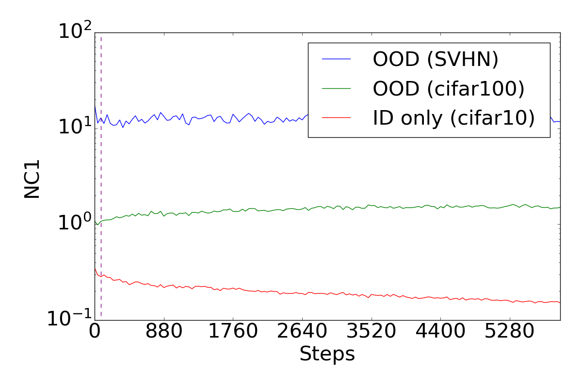
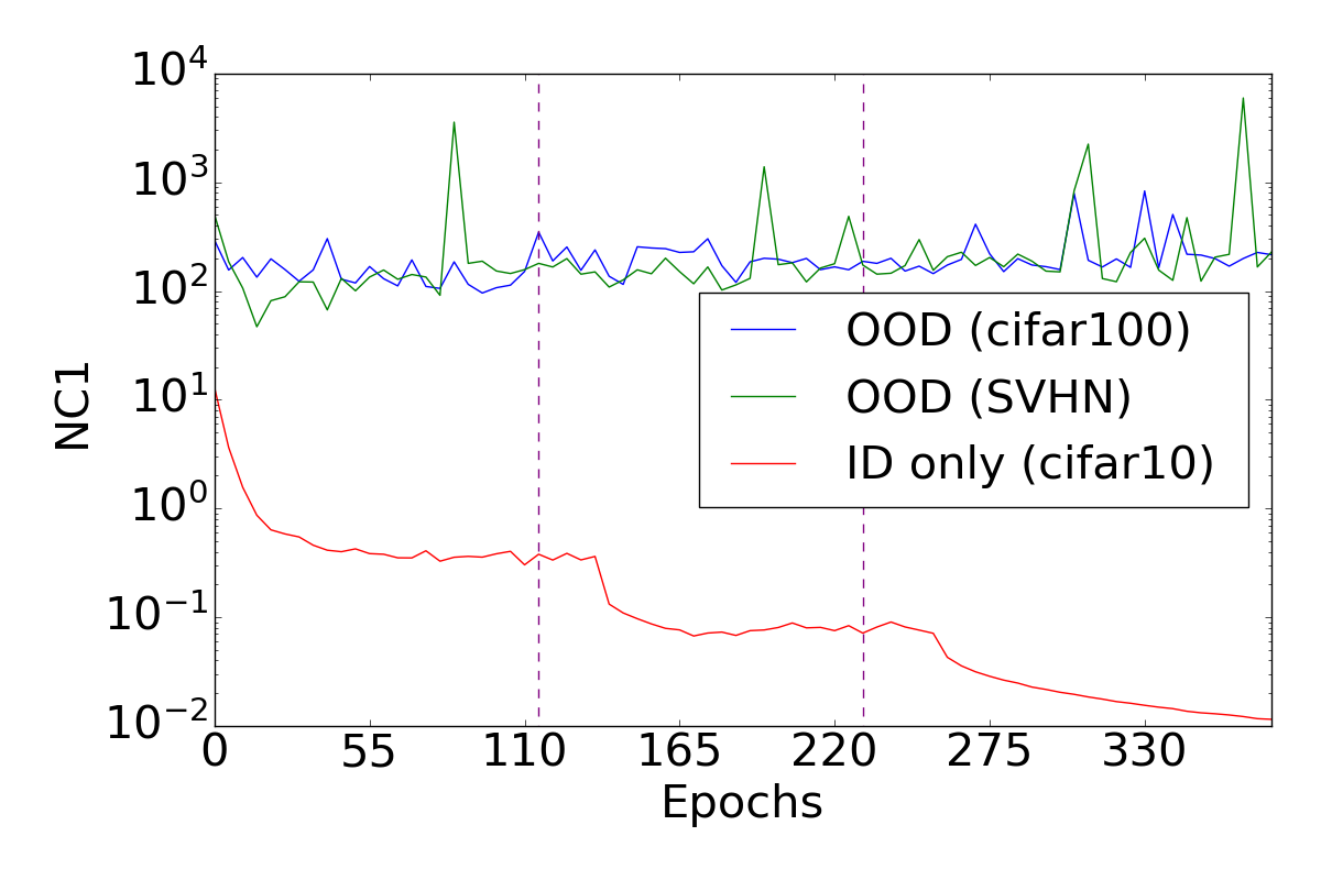
CIFAR-10

(a) ViT-B/16

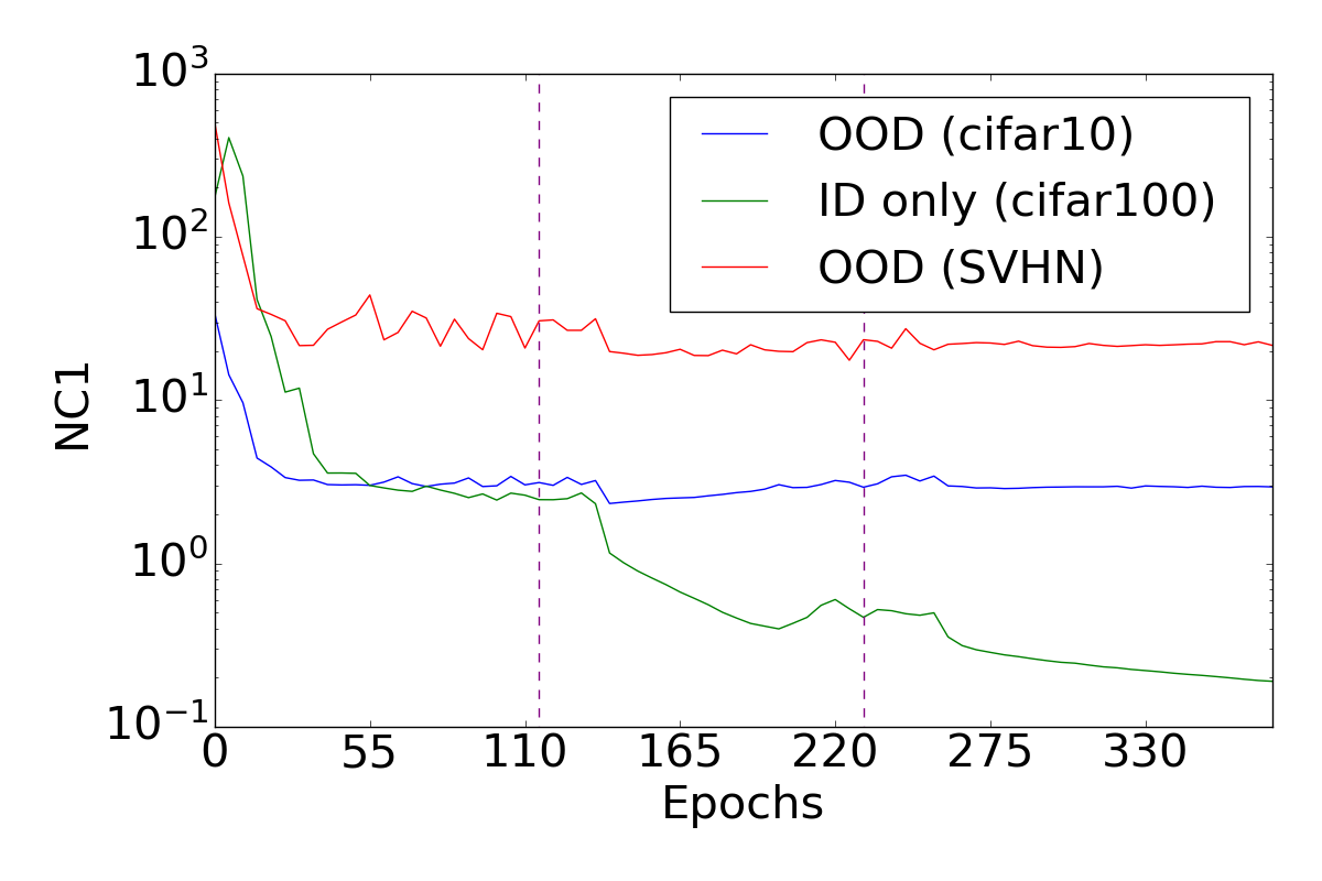
(b) ResNet-18

      CIFAR-100

Figure D.7: Convergence towards variability collapse (NC1) for ID/OOD data separately for ViT-B (left), ResNet-18 (right) both trained on CIFAR-100 as ID. Dashed purple lines indicate the end of warm-up steps in the case of ViT and learning rate decay epochs for ResNet-18.

Convergence of NC2 in presence of OOD.

In order to assess “neural collapse” properties in the presence of OOD data, we investigate the convergence of NC2 equiangularity when the validation set contains OOD data. To this end, for the computation of NC2, we consider the OOD as one supplementary class. Figure D.8 compares the convergence of NC2 when only ID data are used (in dashed black), or when OOD are included as extra classes (in blue and green). In all scenarios the NC2 value tends to converge to a plateau below $0.10$. The examples with OOD data follow the same trend as those without OOD, except for experiments with CIFAR-10 as ID data that have higher NC2 values. According to NC2, this suggests that the equiangularity property between ID clusters and OOD clusters is respected, thus favoring a good separation between ID and OOD data in terms of NECO scores. We are to reinforce this observation in the next paragraph discussing NC5 convergence.

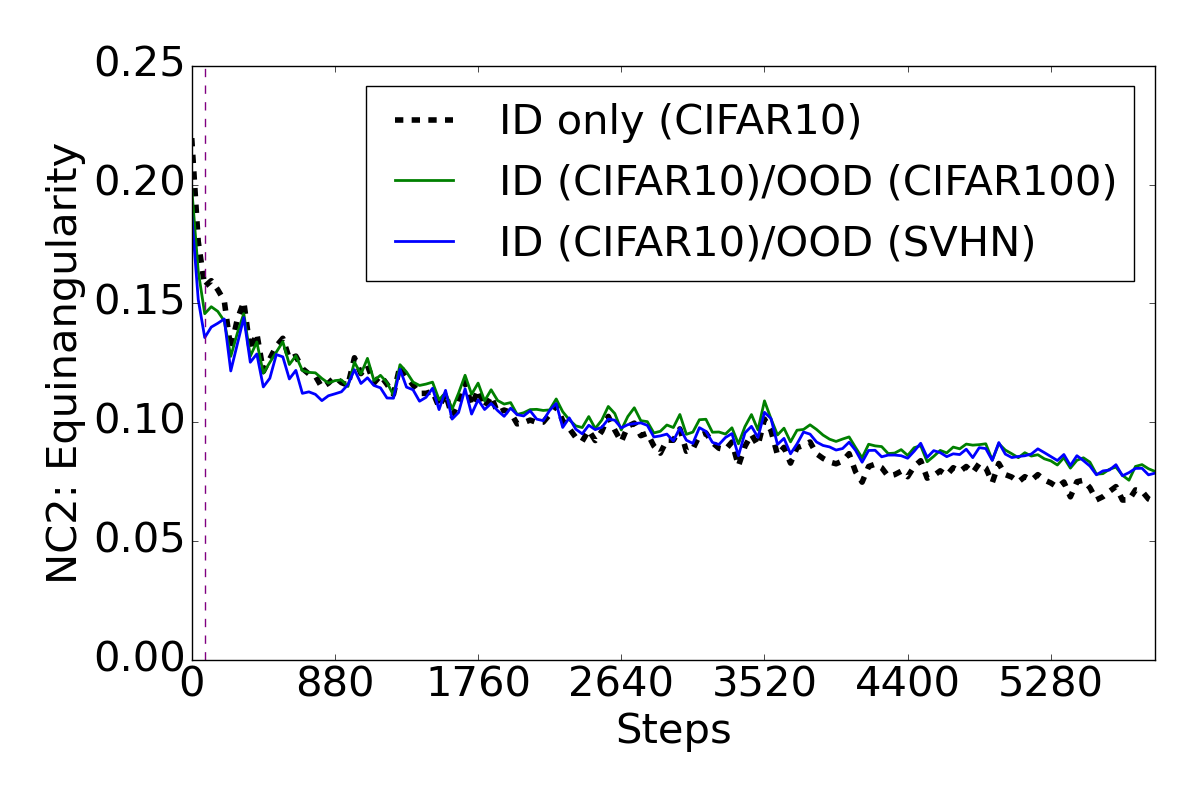
CIFAR-10

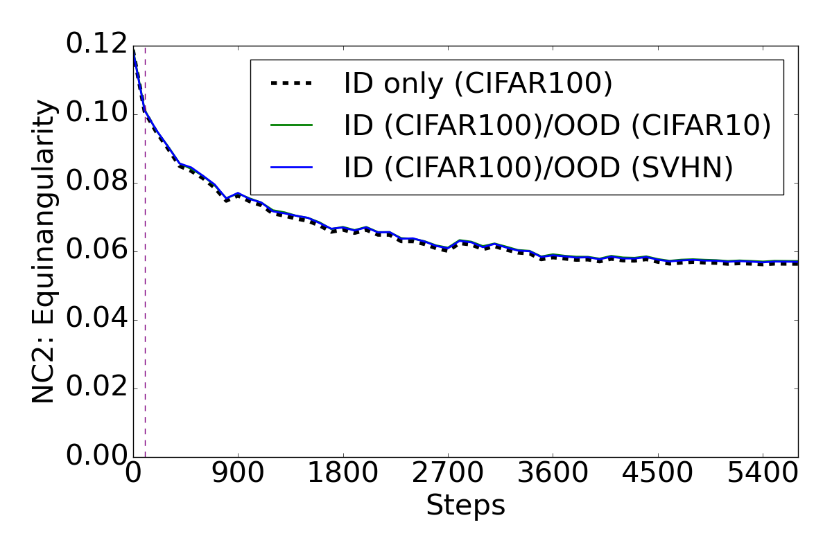
(a)       ViT-B/16

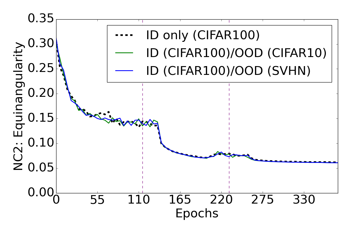
(b) ResNet-18

      CIFAR-100

Figure D.8: Convergence of NC2 for the ID/OOD Equiangularity — in the presence of OOD data— for ViT-B (left), ResNet-18 (right) both trained on CIFAR-10 as ID. Dashed purple lines indicate the end of warm-up steps in the case of ViT and learning rate decay epochs for ResNet-18.

As for the second part of NC2, the equinormality property, its convergence on the mix of ID/OOD data is not relevant to OOD detection. Since if NC5 is verified, the norm of the OOD data will be reduced to zero in the NECO score. However, in order to guarantee an unbiased score towards any ID class, NC2 equinormality needs to be verified on the set of ID data. Since if an ID data cluster has a smaller norm than the others, it is more likely that it will be mistaken as OOD, since its closer to the null vector. Figure D.9 shows the convergence of this property on our ID data, hence guarantying an unbiased score.

CIFAR-10

(a)       ViT-B/16

(b) ResNet-18

      CIFAR-100

Figure D.9: Convergence of NC2 equinormality on ID data for ViT-B (left), ResNet-18 (right) both trained on CIFAR-10 as ID. Dashed purple lines indicate the end of warm-up steps in the case of ViT and learning rate decay epochs for ResNet-18.

Convergence of NC5.

Figure D.10 illustrates the convergence of NC5 when CIFAR-10 or CIFAR-100 are used as ID datasets. In all cases, we observe for both models ( i.e., ViT-B/16 and ResNet-18) very low values for NC5 (Equation 7). Hence, according to our hypothesis, the models tend to maximize the ID/OOD othogonality as we reach the TPT. While all cases exhibit convergence of the OrthoDev, we observe that ViT tend to converge to a much lower value than ResNet-18. Hence, this may explain the performance gap between the ViT-B/16 and the ResNet-18 models.

In Section 5 we empirically demonstrate that ViT-B/16 (pretrained on ImageNet-21K) with NECO outperfoms all baseline methods. In Figure D.11 we illustrate the NC5 OrthoDev during the fine tuning process on ImageNet-1K against different OOD datasets (see Section 5 for the dataset details). Despite a very low initial value ($2\times 10^{-1}$ for the worst example), we observe that NC5 tend to slightly decrease. We believe that the low initial value is due to the pretraining on the ImageNet-21K dataset, hence favoring a premature TPT in the fine tuning phase.

CIFAR-10

(a) ViT-B/16

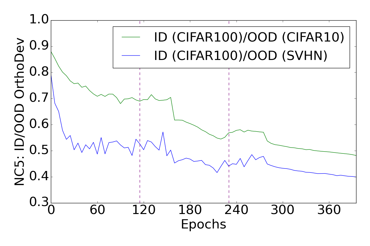
(b) ResNet-18

CIFAR-100

Figure D.10: Convergence of NC5 for the ID/OOD orthogonality— in the presence of OOD data — for ViT-B (left), ResNet-18 (right) both trained on CIFAR-10 (Top) and CIFAR-100 (Bottom) as ID. Dashed purple lines indicate the end of warm-up steps in the case of ViT and learning rate decay epochs for ResNet-18.

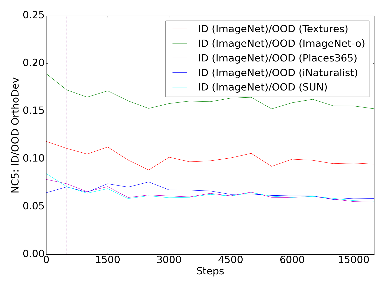
Figure D.11: Convergence towards OrthoDev minimization, for a ViT-B/16 model pre-trained on ImageNet-1K and finetuned on ImageNet-1k. Dashed purple lines indicate the end of warm-up steps.

In Figure D.12, We investigate the neural collapse when the DNN is trained without pretrained weights, and show the convergence of the NC1, NC2 and the NC5. We observe that the curves tend to be steeper than experiments with pretrained weights, reinforcing the hypothesis about the contribution of the pretraining towards reaching the TPT faster. While we are able to reach reasonable performance in the OOD cases, we observe that the NC5 value is slightly higher than experiments with pretrained weights, suggesting their contributions in the neural collapse and its properties for the OOD detection. We hypothesize that this is due to the rich information contained in the pretrained weights that indirectly contributes to the separation in the ETF of the ID from the OOD.

(a) NC1

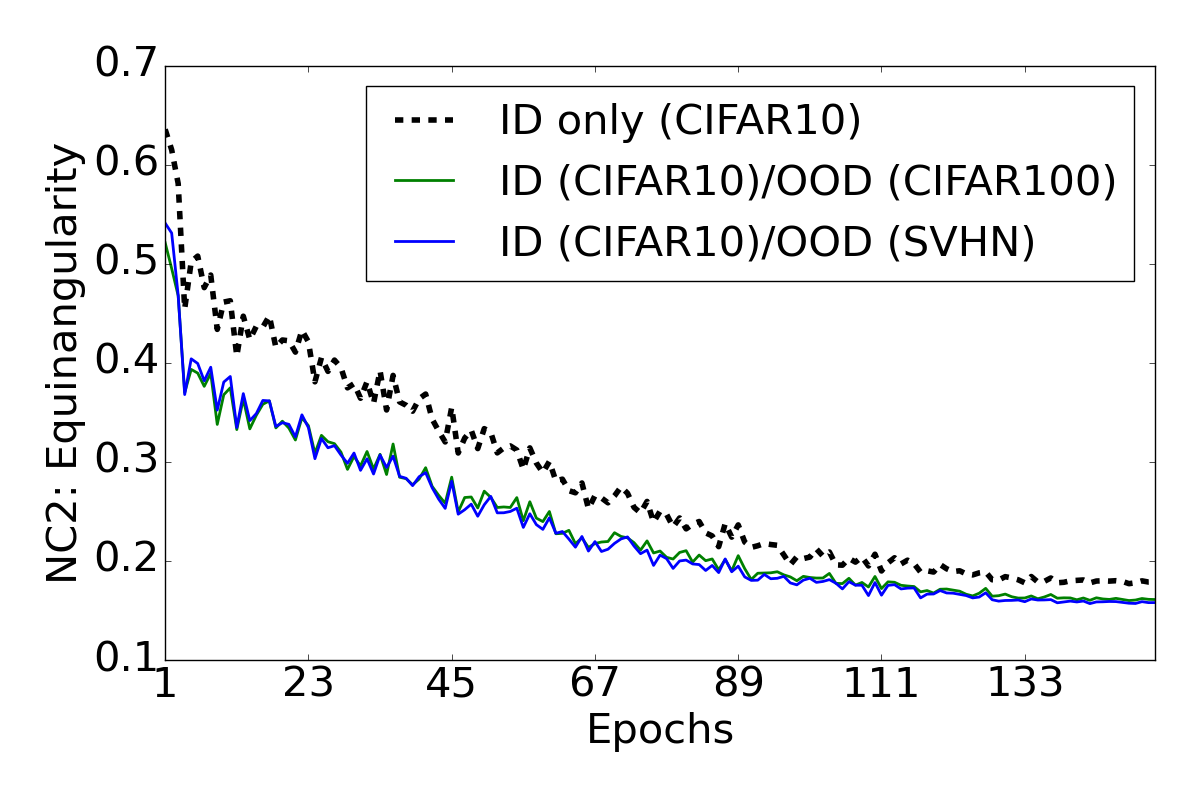
(b) NC2

(c) NC5

Figure D.12: Convergence of variability collapse (NC1), ID/OOD Equiangularity (NC2), and ID/OOD orthogonality (NC5) in the presence of OOD data. A ViT-B/16 is trained (150 epochs) without pre-training on CIFAR-10 , with Top 1% accuracy=72.07%. OOD Performance on CIFAR-10/CIFAR-100: 95.96% AUROC and 13.86% FPR95; on CIFAR-10 vs SVHN:AUROC =99.15% and FPR95 =3.77%

Complementary Feature Projection on Various OOD Datasets

Finally, to further demonstrate the broad pertinence of NECO score, Figure D.13 shows features projection of ID (CIFAR-10) and OOD (CIFAR-100, iNaturalist, SUN, Places365) datasets on the first two principal components of a PCA, fitted on CIFAR-10 ID data. Each class of the ID dataset is colored and the OOD datasets are in gray. As a result of the convergence of the NC1 property, notice how the ID classes are well clustered despite the low dimensional representation. Conversely, the OOD samples are all centered at the null vector position. This suggests that the NECO score for all these cases will be highly separable between ID and OOD data, as we are to discuss in Appendix E.

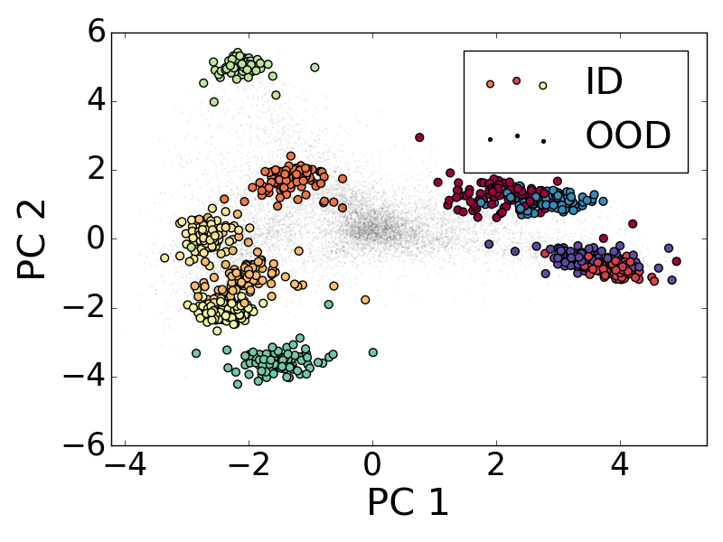
(a) CIFAR-100

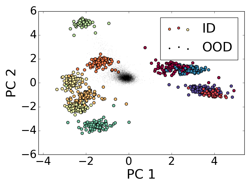
(b) iNaturalist

(c) SUN

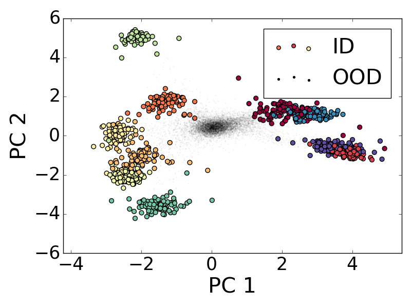
(d) Place365

Figure D.13: Projections on the first two principal components of a PCA fitted on CIFAR-10 using the ViT penultimate layer representation. The colored points indicate the ID dataset classes while the gray points are the OOD.

Appendix E Complementary Results

In this section, we present additional results that extend our findings, with either complementary DNN architectures or OOD benchmarks. The intent is to gain a better understanding on the versatility of our proposed approach, NECO, against different cases.

NECO with DeiT.

Table E.6 presents the results for NECO applied on the DeiT model fine-tuned on ImageNet-1K and evaluated on different datasets against baseline methods. The best performances are highlighted in bold. Contrary to the results with ViT, we observe that on average NECO with DeiT only surpasses the baselines in terms of FPR95.

Model	Method	ImageNet-O AUROC$\uparrow$ FPR$\downarrow$	Textures AUROC$\uparrow$ FPR$\downarrow$	iNaturalist AUROC$\uparrow$ FPR$\downarrow$	SUN AUROC$\uparrow$ FPR$\downarrow$	Places365 AUROC$\uparrow$ FPR$\downarrow$	Average AUROC$\uparrow$ FPR$\downarrow$
DeiT-B/16	Softmax score	63.50 87.70	81.56 65.18	88.44 51.79	81.18 67.64	80.57 69.68	79.05 68.39
	MaxLogit	61.30 85.05	80.32 62.15	85.28 52.99	76.70 67.53	75.74 69.88	75.86 67.52
	Energy	60.59 83.80	77.64 65.27	78.40 65.52	71.23 74.99	69.70 76.53	71.51 73.22
	Energy+ReAct	64.24 82.30	80.25 63.94	84.05 59.69	77.19 69.54	75.78 71.41	76.30 69.37
	ViM	73.93 89.20	78.62 85.67	88.75 71.68	77.70 82.60	76.66 80.04	79.13 81.83
	Residual	72.80 92.15	75.37 89.75	87.08 77.99	75.67 86.33	74.99 83.51	77.18 85.95
	GradNorm	32.79 98.60	38.93 93.85	27.47 98.78	31.21 98.13	30.55 98.39	32.19 97.55
	Mahalanobis	75.37 90.90	81.04 82.45	90.32 67.52	80.95 81.39	80.21 78.80	81.57 80.21
	KL Matching	68.36 84.25	82.20 64.63	89.44 51.81	82.09 73.20	81.09 74.94	80.63 69.76
	ASH-B	46.86 94.05	60.22 85.50	46.24 95.00	35.76 97.45	35.39 96.91	44.89 93.78
	ASH-P	32.21 99.25	24.71 99.06	14.55 99.83	22.36 98.98	23.41 99.21	23.45 99.27
	ASH-S	37.90 95.65	32.85 97.94	19.77 99.65	24.98 97.97	27.13 97.74	28.53 97.79
	NECO (ours)	62.72 84.10	80.82 59.47	89.54 42.26	77.64 65.55	76.48 68.13	77.44 63.90

Table E.6: OOD detection for NECO and baseline methods. The ID dataset is ImageNet-1K, and OOD datasets are Textures, ImageNet-O, iNaturalist, SUN, and Places365. Both metrics AUROC and FPR95 are in percentage. A pre-trained DeiT-B/16 model is tested. The best method is emphasized in bold.

OpenOOD Benchmark — ImageNet-1K Challenge.

OpenOOD is a recent test bench focusing on OOD detection proposing classic test cases from the literature. In this paragraph we focus on the ImageNet-1K challenge with a set of OOD test cases grouped in increasing difficulties: Near-OOD — with SSB-hard (Vaze et al., 2021) and NINCO (Bitterwolf et al., 2023), Far-OOD — with iNaturalist (Horn et al., 2017), Textures (Cimpoi et al., 2014), OpenImage-O (Wang et al., 2022) , Covariate Shift — with ImageNet-C (Hendrycks & Dietterich, 2019), ImageNet-R (Hendrycks et al., 2021a), ImageNet-V2 (Recht et al., 2019). Figure E.14 shows five examples from each of these datasets.

Table E.7 presents our results on each group, including a global average performance. On average over all the test sets, we observe that NECO outperforms all the baseline methods, with all DNN models. With SwinV2, NECO reaches the first rank, in terms of FPR95, and the top3, in terms of AUROC, on all datasets. However, on the global average, ViT with NECO is the best strategy. Although NECO perform relatively well on the Covariate Shift, in particular with SwinV2, but remains limited with ViT.

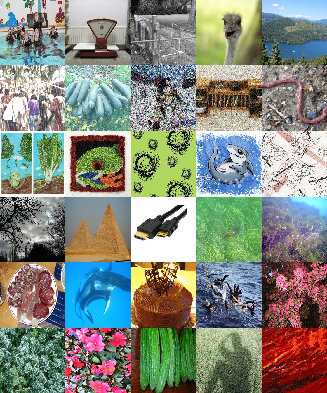
Figure E.14: Example images from OOD datasets with each row representing a dataset: ImageNet-V2,imageNet-C,imageNet-R, NINCO, SSB-hard and OpenImage-O respectively from top to bottom.

		Covariate Shift				Near OOD			Far OOD				Global
Model	Method	ImageNet-V2 AUROC$\uparrow$ FPR$\downarrow$	ImageNet-C AUROC$\uparrow$ FPR$\downarrow$	ImageNet-R AUROC$\uparrow$ FPR$\downarrow$	Average AUROC$\uparrow$ FPR$\downarrow$	NINCO AUROC$\uparrow$ FPR$\downarrow$	SSB-hard AUROC$\uparrow$ FPR$\downarrow$	Average AUROC$\uparrow$ FPR$\downarrow$	Textures AUROC$\uparrow$ FPR$\downarrow$	iNaturalist AUROC$\uparrow$ FPR$\downarrow$	open-images AUROC$\uparrow$ FPR$\downarrow$	Average AUROC$\uparrow$ FPR$\downarrow$	Average AUROC$\uparrow$ FPR$\downarrow$
ViT	Softmax score	58.61 89.37	71.75 71.02	81.42 56.82	70.59 72.40	88.97 46.67	80.31 66.03	84.64 56.35	86.64 49.40	97.21 12.14	93.08 29.62	92.31 30.39	82.25 52.63
	MaxLogit	58.71 88.90	73.64 69.46	86.65 47.16	73.00 68.51	92.91 35.40	87.28 53.10	90.09 44.25	91.69 36.90	98.87 5.72	96.75 17.33	95.77 19.98	85.81 44.25
	Energy	58.59 89.20	73.54 69.69	87.12 44.52	73.08 67.80	93.13 33.51	87.88 49.16	90.50 41.34	92.13 34.15	99.04 4.76	97.13 14.67	96.10 17.86	86.07 42.46
	Energy+ReAct	58.57 89.32	73.37 69.82	86.93 44.92	72.96 68.02	93.10 33.43	87.60 49.74	90.35 41.59	92.08 34.50	99.02 4.91	97.13 14.76	96.08 18.06	85.97 42.67
	ViM	57.33 90.38	70.10 80.80	86.26 52.61	71.23 74.60	93.12 32.36	88.30 45.11	90.71 38.73	91.63 38.22	99.59 2.00	97.13 15.90	96.12 18.71	85.43 44.67
	Residual	55.18 92.55	62.81 90.03	81.90 69.06	66.63 83.88	89.95 44.96	85.38 51.62	87.67 48.29	87.71 52.34	99.36 2.79	94.84 25.77	93.97 26.97	82.14 53.64
	GradNorm	54.45 89.64	69.44 68.69	76.54 46.91	66.81 68.41	84.21 37.14	80.89 51.11	82.55 44.12	86.29 35.76	97.45 6.17	93.74 16.61	92.49 19.51	80.38 44.00
	Mahalanobis	58.24 90.07	70.93 77.45	86.52 48.82	71.90 72.11	93.90 30.32	85.72 50.22	89.81 40.27	91.69 37.93	99.67 1.55	97.36 14.40	96.24 17.96	85.50 43.84
	KL-Matching	54.98 90.09	65.36 73.41	76.24 59.06	65.53 74.19	84.30 51.24	70.92 69.70	77.61 60.47	84.61 52.38	95.07 15.31	90.22 35.32	89.97 34.34	77.71 55.81
	ASH-B	48.70 94.28	44.13 93.79	57.90 89.28	50.24 92.45	57.30 89.09	57.23 92.61	57.27 90.85	66.05 83.29	72.62 80.62	68.34 83.42	69.00 82.44	59.03 88.30
	ASH-P	56.55 91.16	69.94 77.33	86.18 47.98	70.89 72.16	91.27 36.49	89.38 39.29	90.33 37.89	91.55 37.58	98.75 6.25	96.45 18.10	95.58 20.64	85.01 44.27
	ASH-S	55.88 91.29	68.85 78.88	85.23 50.25	69.99 73.47	90.34 37.67	89.30 37.99	89.82 37.83	91.00 39.73	98.50 7.28	95.97 19.41	95.16 22.14	84.38 45.31
	NECO (ours)	58.69 89.00	73.48 69.57	86.45 47.96	72.87 68.84	93.38 30.98	87.52 41.54	90.45 36.26	92.86 32.44	99.34 3.26	97.55 12.99	96.58 16.23	86.16 40.97
SwinV2	Softmax score	57.76 90.14	75.99 67.42	78.35 64.50	70.70 74.02	78.54 71.91	70.54 82.39	74.54 77.15	81.72 60.91	88.59 47.66	85.08 57.70	85.13 55.42	77.07 67.83
	MaxLogit	56.77 90.42	75.41 65.83	76.65 63.83	69.61 73.36	74.80 73.39	66.68 83.64	70.74 78.52	80.36 59.55	86.47 50.51	82.45 58.75	83.09 56.27	74.95 68.24
	Energy	55.73 91.22	73.96 67.44	74.23 68.22	67.97 75.63	70.36 78.70	62.84 86.50	66.60 82.60	77.91 64.44	81.85 63.44	78.37 66.58	79.38 64.82	71.91 73.32
	Energy+ReAct	56.76 90.77	75.71 66.57	79.16 61.41	70.54 72.92	74.73 75.23	65.38 85.70	70.06 80.47	84.56 59.86	90.23 51.97	84.72 59.51	86.50 57.11	76.41 68.88
	ViM	56.29 90.88	68.09 82.40	83.09 55.67	69.16 76.32	74.55 77.97	65.33 87.30	69.94 82.64	81.50 61.18	87.54 54.09	85.66 55.86	84.90 57.04	75.26 70.67
	Residual	55.25 91.59	62.84 85.38	80.62 59.69	66.24 78.89	70.95 80.49	62.68 88.64	66.81 84.56	77.36 65.00	83.23 59.77	81.72 60.75	80.77 61.84	71.83 73.91
	GradNorm	45.78 95.52	48.37 86.71	27.00 97.20	40.38 93.14	34.90 95.34	40.76 95.65	37.83 95.50	33.84 93.31	31.82 95.01	29.53 95.38	31.73 94.57	36.50 94.27
	Mahalanobis	57.14 90.83	70.04 83.55	84.58 55.69	70.59 76.69	78.76 79.11	68.94 88.37	73.85 83.74	84.51 63.35	89.81 57.10	88.20 58.95	87.51 59.80	77.75 72.12
	KL-Matching	54.74 90.95	64.08 81.73	73.40 70.87	64.07 81.18	72.29 75.40	62.96 83.82	67.62 79.61	75.30 71.69	82.93 58.29	80.26 65.74	79.50 65.24	70.75 74.81
	ASH-B	50.67 95.66	52.07 94.49	50.13 97.54	50.96 95.90	53.33 96.70	55.91 94.86	54.62 95.78	38.59 97.50	48.62 97.55	48.00 97.75	45.07 97.60	49.66 96.51
	ASH-P	45.39 95.91	36.69 96.14	25.86 98.51	35.98 96.85	29.17 98.37	37.20 97.51	33.19 97.94	26.51 98.90	20.73 99.28	22.35 99.22	23.20 99.13	30.49 97.98
	ASH-S	45.17 95.35	36.40 94.49	27.52 95.78	36.36 95.21	28.09 97.23	33.85 97.05	30.97 97.14	36.08 94.63	16.15 99.50	22.91 97.08	25.05 97.07	30.77 96.39
	NECO (ours)	58.04 89.86	77.16 63.05	83.67 56.36	72.96 69.76	77.95 66.69	70.63 79.47	74.29 73.08	82.27 54.67	91.89 34.41	86.98 47.96	87.05 45.68	78.57 61.56
DeiT	Softmax score	58.05 90.54	75.42 71.27	78.48 64.85	70.65 75.55	79.20 72.81	70.56 84.10	74.88 78.45	81.56 65.18	88.44 51.79	84.64 61.14	84.88 59.37	77.04 70.21
	MaxLogit	56.84 90.33	75.55 67.31	75.40 62.66	69.26 73.43	75.08 72.18	67.11 84.33	71.09 78.25	80.32 62.15	85.28 52.99	80.74 60.06	82.11 58.40	74.54 69.00
	Energy	55.55 90.77	74.25 67.74	72.22 65.16	67.34 74.56	69.82 76.91	62.65 87.05	66.23 81.98	77.64 65.27	78.40 65.52	75.24 66.53	77.09 65.77	70.72 73.12
	Energy+ReAct	56.66 90.41	75.55 67.87	77.09 60.72	69.77 73.00	74.08 75.20	65.21 86.29	69.64 80.75	80.25 63.94	84.05 59.69	80.55 62.72	81.62 62.12	74.18 70.86
	ViM	56.49 90.03	65.68 91.97	84.79 59.56	68.99 80.52	78.20 81.56	64.45 91.12	71.33 86.34	78.62 85.67	88.75 71.68	86.40 75.08	84.59 77.48	75.42 80.83
	Residual	55.85 90.43	61.01 93.69	83.74 66.02	66.87 83.38	76.21 84.50	62.88 92.23	69.55 88.36	75.37 89.75	87.08 77.99	84.55 80.07	82.33 82.60	73.34 84.33
	GradNorm	46.54 94.62	56.39 80.16	26.00 98.43	42.98 91.07	34.63 97.48	43.45 95.91	39.04 96.69	60.22 85.50	46.24 95.00	27.40 97.89	44.62 92.80	42.61 93.12
	Mahalanobis	57.43 90.36	66.96 91.50	85.37 56.87	69.92 79.58	80.75 80.91	67.72 91.08	74.23 86.00	24.71 99.06	14.55 99.83	88.01 72.18	42.42 90.36	60.69 85.22
	KL-Matching	55.85 91.31	71.39 78.53	79.96 67.42	69.07 79.09	79.46 74.04	68.14 83.56	73.80 78.80	32.85 97.94	19.77 99.65	86.47 61.26	46.36 86.28	61.74 81.71
	ASH-B	46.88 94.53	40.66 97.00	46.99 89.40	44.84 93.64	41.14 96.50	34.89 98.28	38.02 97.39	38.93 93.85	27.47 98.78	40.78 94.89	35.73 95.84	39.72 95.40
	ASH-P	44.55 95.69	35.21 96.49	19.57 99.12	33.11 97.10	26.30 99.44	39.02 97.10	32.66 98.27	81.04 82.45	90.32 67.52	17.73 99.35	63.03 83.11	44.22 92.14
	ASH-S	48.35 94.91	30.08 96.88	41.46 95.86	39.96 95.88	31.88 97.69	36.75 96.91	34.31 97.30	82.20 64.63	89.44 51.81	27.41 98.04	66.35 71.49	48.45 87.09
	NECO (ours)	57.28 90.13	76.20 63.80	75.40 63.55	69.63 72.49	78.15 66.88	68.24 80.60	73.19 73.74	80.82 59.47	89.54 42.26	81.88 57.70	84.08 53.14	75.94 65.55

Table E.7: OOD detection for NECO against baseline methods, on the ImageNet-1K challenge from openOOD benchmark (Zhang et al., 2023) that includes: open-image, ImageNet-V2, ImageNet-R, ImageNet-C, NINCO, SSB-hard, Textures and iNaturalist. Both metrics AUROC and FPR95. are in percentage.Three architectures (ViT with fine tuning on ImageNet-1K, SwinV2, and DeiT) are evaluated. The best method is emphasized in bold, and the 2nd and 3rd ones are underlined.

Distribution of NECO Values.

To verify the discrepancy in the distribution of NECO scores between ID and OOD values, Figure E.15 depicts the density score histograms for the ImageNet benchmark when using ViT and Swin models. These histograms reveal a significant degree of separation in certain cases, such as when iNaturalist is used as the OOD dataset with the ViT model. However, in some other cases, like when ImageNet-O is employed as the OOD dataset with the Swin model, the separation remains less pronounced. Across all the presented scenarios, ViT-B consistently outperforms other variants of vision transformers in the OOD detection task. This observation leads us to hypothesize that ViT-B exhibits more collapse than its counterparts, although further testing is needed to draw definitive conclusions.

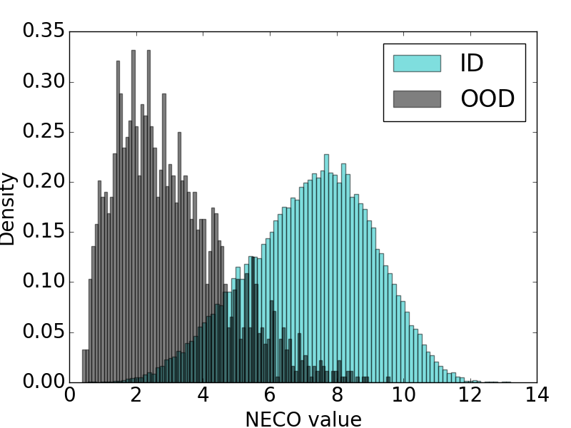
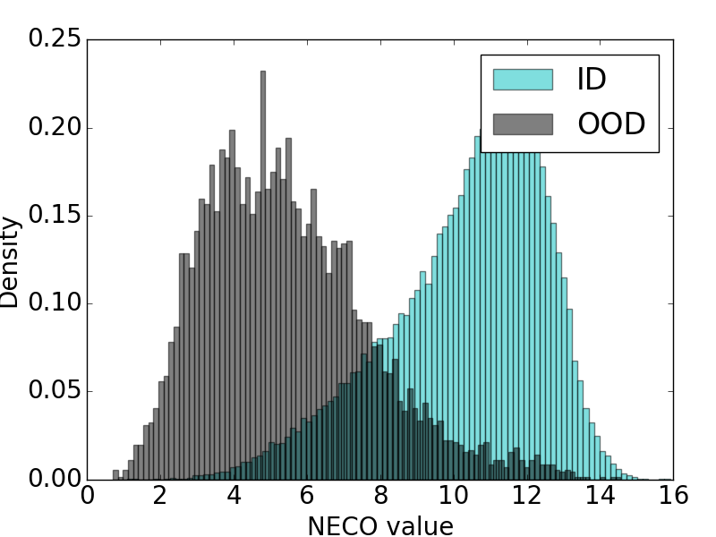
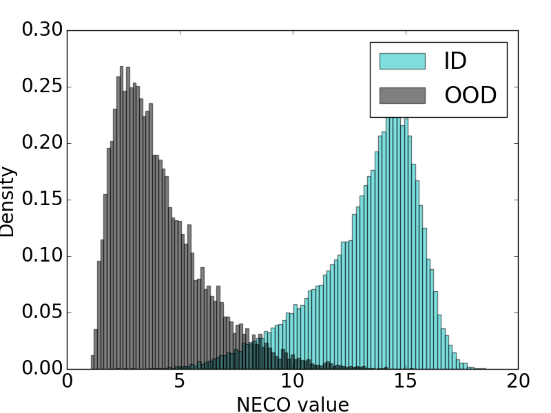
(a) ViT-B/16

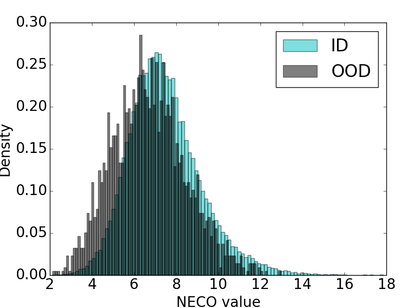
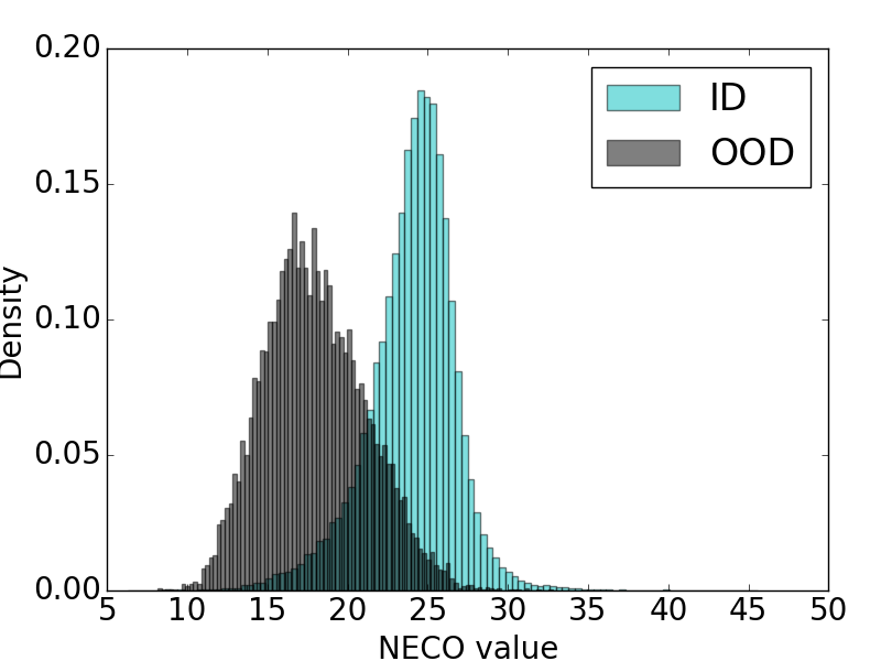
(b) SwinV2-B/16

Figure E.15: ID (ImageNet) and OOD ImageNet-O (left), Textures (center) and iNaturalist (right) NECO score distributions.

Similarly, figure E.17 presents the density score histograms for the CIFAR-10/CIFAR-100 benchmark when using ViT and ResNet-18 models, respectively. In certain cases, such as CIFAR-10 (ID)/SVHN (OOD) with the ViT model, these histograms reveal nearly perfect separation. However, achieving separation becomes notably more challenging in the case of CIFAR-100 (ID)/CIFAR-10 (OOD). This difficulty arises because CIFAR-10 shares labels with a subset of the CIFAR-100 dataset, causing their data clusters to be much closer. This effect is particularly pronounced when using a ResNet-18 model compared to a ViT. The superior performance of the ViT model is further highlighted by its significantly lower values across all “neural collapse” metrics.

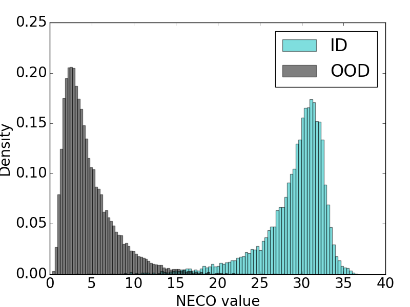
CIFAR-10 vs SVHN

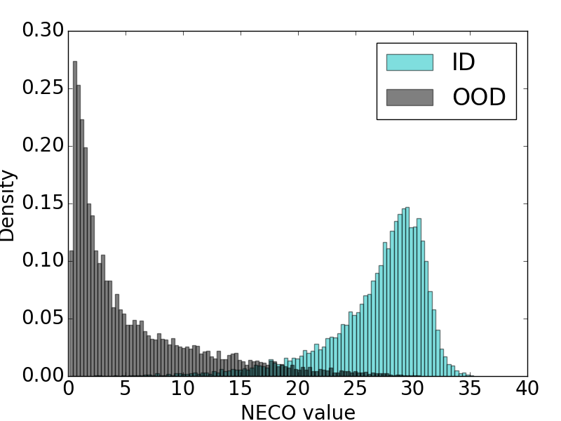
CIFAR-10 vs CIFAR-100

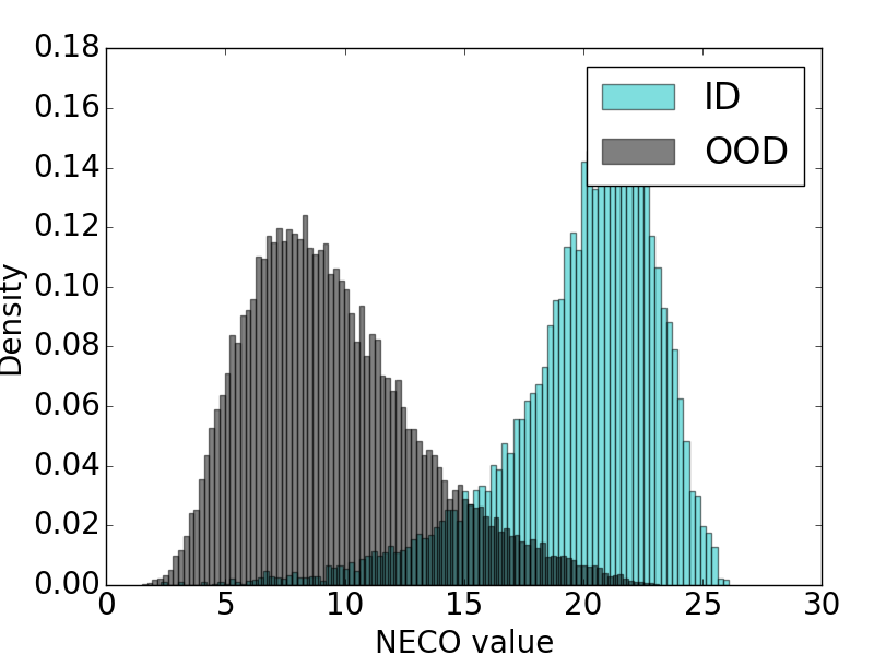
CIFAR-100 vs SVHN

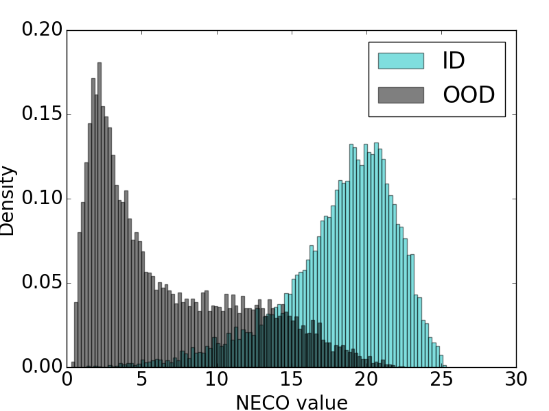
CIFAR-100 vs CIFAR-10

ViT-B/16

CIFAR-10 vs SVHN

CIFAR-10 vs CIFAR-100

CIFAR-100 vs SVHN

CIFAR-100 vs CIFAR-10

ResNet-18

Figure E.17: NECO score distributions for different ID and OOD tuples, with a ViT-B/16 (left) and ResNet-18 (right) both fine tuned on the ID training dataset.

References

- Abati et al. (2019) Davide Abati, Angelo Porrello, Simone Calderara, and Rita Cucchiara. Latent space autoregression for novelty detection, 2019.
- Bitterwolf et al. (2023) Julian Bitterwolf, Maximilian Müller, and Matthias Hein. In or out? fixing imagenet out-of-distribution detection evaluation, 2023.
- Cimpoi et al. (2014) Mircea Cimpoi, Subhransu Maji, Iasonas Kokkinos, Sammy Mohamed, and Andrea Vedaldi. Describing textures in the wild. In Proceedings of the IEEE Conference on Computer Vision and Pattern Recognition (CVPR), June 2014.
- Cook et al. (2020) Matthew Cook, Alina Zare, and Paul Gader. Outlier detection through null space analysis of neural networks. arXiv preprint arXiv:2007.01263, 2020.
- Deng (2012) Li Deng. The mnist database of handwritten digit images for machine learning research. IEEE Signal Processing Magazine, 29(6):141–142, 2012.
- DeVries & Taylor (2018) Terrance DeVries and Graham W. Taylor. Learning confidence for out-of-distribution detection in neural networks, 2018.
- Djurisic et al. (2022) Andrija Djurisic, Nebojsa Bozanic, Arjun Ashok, and Rosanne Liu. Extremely simple activation shaping for out-of-distribution detection. arXiv preprint arXiv:2209.09858, 2022.
- Dosovitskiy et al. (2020) Alexey Dosovitskiy, Lucas Beyer, Alexander Kolesnikov, Dirk Weissenborn, Xiaohua Zhai, Thomas Unterthiner, Mostafa Dehghani, Matthias Minderer, Georg Heigold, Sylvain Gelly, Jakob Uszkoreit, and Neil Houlsby. An image is worth 16x16 words: Transformers for image recognition at scale. CoRR, abs/2010.11929, 2020. URL https://arxiv.org/abs/2010.11929.
- Ergen & Pilanci (2021) Tolga Ergen and Mert Pilanci. Revealing the structure of deep neural networks via convex duality, 2021.
- Fort et al. (2021) Stanislav Fort, Jie Ren, and Balaji Lakshminarayanan. Exploring the limits of out-of-distribution detection. CoRR, abs/2106.03004, 2021. URL https://arxiv.org/abs/2106.03004.
- Haas et al. (2023) Jarrod Haas, William Yolland, and Bernhard T Rabus. Linking neural collapse and l2 normalization with improved out-of-distribution detection in deep neural networks. Transactions on Machine Learning Research, 2023. ISSN 2835-8856. URL https://openreview.net/forum?id=fjkN5Ur2d6.
- Han et al. (2022) X. Y. Han, Vardan Papyan, and David L. Donoho. Neural collapse under mse loss: Proximity to and dynamics on the central path, 2022.
- He et al. (2015) Kaiming He, Xiangyu Zhang, Shaoqing Ren, and Jian Sun. Deep residual learning for image recognition. CoRR, abs/1512.03385, 2015. URL http://arxiv.org/abs/1512.03385.
- He et al. (2016) Kaiming He, Xiangyu Zhang, Shaoqing Ren, and Jian Sun. Deep residual learning for image recognition. In 2016 IEEE Conference on Computer Vision and Pattern Recognition (CVPR), pp. 770–778, 2016. doi: 10.1109/CVPR.2016.90.
- Hendrycks & Dietterich (2019) Dan Hendrycks and Thomas Dietterich. Benchmarking neural network robustness to common corruptions and perturbations. arXiv preprint arXiv:1903.12261, 2019.
- Hendrycks & Gimpel (2017) Dan Hendrycks and Kevin Gimpel. A baseline for detecting misclassified and out-of-distribution examples in neural networks. Proceedings of International Conference on Learning Representations, 2017.
- Hendrycks et al. (2018) Dan Hendrycks, Mantas Mazeika, and Thomas G. Dietterich. Deep anomaly detection with outlier exposure. CoRR, abs/1812.04606, 2018. URL http://arxiv.org/abs/1812.04606.
- Hendrycks et al. (2021a) Dan Hendrycks, Steven Basart, Norman Mu, Saurav Kadavath, Frank Wang, Evan Dorundo, Rahul Desai, Tyler Zhu, Samyak Parajuli, Mike Guo, et al. The many faces of robustness: A critical analysis of out-of-distribution generalization. In Proceedings of the IEEE/CVF International Conference on Computer Vision, pp. 8340–8349, 2021a.
- Hendrycks et al. (2021b) Dan Hendrycks, Kevin Zhao, Steven Basart, Jacob Steinhardt, and Dawn Song. Natural adversarial examples. In Proceedings of the IEEE/CVF Conference on Computer Vision and Pattern Recognition (CVPR), pp. 15262–15271, June 2021b.
- Hendrycks et al. (2022) Dan Hendrycks, Steven Basart, Mantas Mazeika, Mohammadreza Mostajabi, Jacob Steinhardt, and Dawn Xiaodong Song. Scaling out-of-distribution detection for real-world settings. In International Conference on Machine Learning, 2022. URL https://api.semanticscholar.org/CorpusID:227407829.
- Horn et al. (2017) Grant Van Horn, Oisin Mac Aodha, Yang Song, Alexander Shepard, Hartwig Adam, Pietro Perona, and Serge J. Belongie. The inaturalist challenge 2017 dataset. CoRR, abs/1707.06642, 2017. URL http://arxiv.org/abs/1707.06642.
- Huang et al. (2017) Gao Huang, Zhuang Liu, Laurens Van Der Maaten, and Kilian Q. Weinberger. Densely connected convolutional networks. In 2017 IEEE Conference on Computer Vision and Pattern Recognition (CVPR), pp. 2261–2269, 2017. doi: 10.1109/CVPR.2017.243.
- Huang & Li (2021a) Rui Huang and Yixuan Li. Mos: Towards scaling out-of-distribution detection for large semantic space. In Proceedings of the IEEE/CVF Conference on Computer Vision and Pattern Recognition (CVPR), pp. 8710–8719, June 2021a.
- Huang & Li (2021b) Rui Huang and Yixuan Li. Mos: Towards scaling out-of-distribution detection for large semantic space, 2021b.
- Huang et al. (2021) Rui Huang, Andrew Geng, and Yixuan Li. On the importance of gradients for detecting distributional shifts in the wild. CoRR, abs/2110.00218, 2021. URL https://arxiv.org/abs/2110.00218.
- Ishida et al. (2020) Takashi Ishida, Ikko Yamane, Tomoya Sakai, Gang Niu, and Masashi Sugiyama. Do we need zero training loss after achieving zero training error? CoRR, abs/2002.08709, 2020. URL https://arxiv.org/abs/2002.08709.
- Jumper et al. (2021) John Jumper, Richard Evans, Alexander Pritzel, and et al. Highly accurate protein structure prediction with AlphaFold. Nature, 596:583–589, 2021. doi: 10.1038/s41586-021-03819-2. URL https://www.nature.com/articles/s41586-021-03819-2.
- Kitt et al. (2010) Bernd Kitt, Andreas Geiger, and Henning Lategahn. Visual odometry based on stereo image sequences with ransac-based outlier rejection scheme. In Intelligent Vehicles Symposium, pp. 486–492. IEEE, 2010. URL http://dblp.uni-trier.de/db/conf/ivs/ivs2010.html#KittGL10.
- Kothapalli (2023) Vignesh Kothapalli. Neural collapse: A review on modelling principles and generalization, 2023.
- Krizhevsky (2012) Alex Krizhevsky. Learning multiple layers of features from tiny images. University of Toronto, 05 2012.
- Lee et al. (2018a) Kimin Lee, Kibok Lee, Honglak Lee, and Jinwoo Shin. A simple unified framework for detecting out-of-distribution samples and adversarial attacks. In S. Bengio, H. Wallach, H. Larochelle, K. Grauman, N. Cesa-Bianchi, and R. Garnett (eds.), Advances in Neural Information Processing Systems, volume 31. Curran Associates, Inc., 2018a. URL https://proceedings.neurips.cc/paper_files/paper/2018/file/abdeb6f575ac5c6676b747bca8d09cc2-Paper.pdf.
- Lee et al. (2018b) Kimin Lee, Kibok Lee, Honglak Lee, and Jinwoo Shin. A simple unified framework for detecting out-of-distribution samples and adversarial attacks. In S. Bengio, H. Wallach, H. Larochelle, K. Grauman, N. Cesa-Bianchi, and R. Garnett (eds.), Advances in Neural Information Processing Systems, volume 31. Curran Associates, Inc., 2018b. URL https://proceedings.neurips.cc/paper_files/paper/2018/file/abdeb6f575ac5c6676b747bca8d09cc2-Paper.pdf.
- Liang et al. (2018) Shiyu Liang, Yixuan Li, and R. Srikant. Enhancing the reliability of out-of-distribution image detection in neural networks. In International Conference on Learning Representations, 2018. URL https://openreview.net/forum?id=H1VGkIxRZ.
- Liu et al. (2020) Weitang Liu, Xiaoyun Wang, John Douglas Owens, and Yixuan Li. Energy-based out-of-distribution detection. ArXiv, abs/2010.03759, 2020. URL https://api.semanticscholar.org/CorpusID:222208700.
- Liu et al. (2021) Ze Liu, Han Hu, Yutong Lin, Zhuliang Yao, Zhenda Xie, Yixuan Wei, Jia Ning, Yue Cao, Zheng Zhang, Li Dong, Furu Wei, and Baining Guo. Swin transformer V2: scaling up capacity and resolution. CoRR, abs/2111.09883, 2021. URL https://arxiv.org/abs/2111.09883.
- Ming et al. (2023) Yifei Ming, Yiyou Sun, Ousmane Dia, and Yixuan Li. How to exploit hyperspherical embeddings for out-of-distribution detection? In The Eleventh International Conference on Learning Representations, 2023. URL https://openreview.net/forum?id=aEFaE0W5pAd.
- Mixon et al. (2020) Dustin G. Mixon, Hans Parshall, and Jianzong Pi. Neural collapse with unconstrained features, 2020.
- Netzer et al. (2011) Yuval Netzer, Tao Wang, Adam Coates, A. Bissacco, Bo Wu, and A. Ng. Reading digits in natural images with unsupervised feature learning. In Proceedings of the NIPS Workshop on Deep Learning and Unsupervised Feature Learning, 2011. URL https://api.semanticscholar.org/CorpusID:16852518.
- OpenAI (2023) OpenAI. Gpt-3, 2023. URL https://openai.com/. Computer software.
- Papyan V (2020) Donoho DL. Papyan V, Han XY. Prevalence of neural collapse during the terminal phase of deep learning training. Computer Vision and Pattern Recognition, 2020.
- Paul Bergmann & Stege (2019) David Sattlegger Paul Bergmann, Michael Fauser and Carsten Stege. Mvtec ad — a comprehensive real-world dataset for unsupervised anomaly detection. Proceedings of the IEEE/CVF Conference on Computer Vision and Pattern Recognition, pp. 9592–9600, 2019.
- Ramesh et al. (2021) Aditya Ramesh, Mukul Goyal, Daniel Summers-Stay, and et al. Dall·e: Creating images from text. arXiv preprint arXiv:2102.12092, 2021. URL https://arxiv.org/abs/2102.12092.
- Recht et al. (2019) Benjamin Recht, Rebecca Roelofs, Ludwig Schmidt, and Vaishaal Shankar. Do imagenet classifiers generalize to imagenet? In International conference on machine learning, pp. 5389–5400. PMLR, 2019.
- Ren et al. (2021) Jie Ren, Stanislav Fort, Jeremiah Liu, Abhijit Guha Roy, Shreyas Padhy, and Balaji Lakshminarayanan. A simple fix to mahalanobis distance for improving near-ood detection, 2021.
- Russakovsky et al. (2015) Olga Russakovsky, Jia Deng, Hao Su, Jonathan Krause, Sanjeev Satheesh, Sean Ma, Zhiheng Huang, Andrej Karpathy, Aditya Khosla, Michael Bernstein, Alexander C. Berg, and Li Fei-Fei. ImageNet Large Scale Visual Recognition Challenge. International Journal of Computer Vision (IJCV), 115(3):211–252, 2015. doi: 10.1007/s11263-015-0816-y.
- Sabokrou et al. (2018) Mohammad Sabokrou, Mohammad Khalooei, Mahmood Fathy, and Ehsan Adeli. Adversarially learned one-class classifier for novelty detection, 2018.
- Schlegl et al. (2017) Thomas Schlegl, Philipp Seeböck, Sebastian M Waldstein, Ursula Schmidt-Erfurth, and Georg Langs. Unsupervised anomaly detection with generative adversarial networks to guide marker discovery. In International conference on information processing in medical imaging, pp. 146–157. Springer, 2017.
- Simonyan & Zisserman (2015) Karen Simonyan and Andrew Zisserman. Very deep convolutional networks for large-scale image recognition, 2015.
- Sun & Li (2022) Yiyou Sun and Yixuan Li. Dice: Leveraging sparsification for out-of-distribution detection. In European Conference on Computer Vision, 2022.
- Sun et al. (2021) Yiyou Sun, Chuan Guo, and Yixuan Li. React: Out-of-distribution detection with rectified activations. In A. Beygelzimer, Y. Dauphin, P. Liang, and J. Wortman Vaughan (eds.), Advances in Neural Information Processing Systems, 2021. URL https://openreview.net/forum?id=IBVBtz_sRSm.
- Sun et al. (2022) Yiyou Sun, Yifei Ming, Xiaojin Zhu, and Yixuan Li. Out-of-distribution detection with deep nearest neighbors, 2022.
- Techapanurak et al. (2019) Engkarat Techapanurak, Masanori Suganuma, and Takayuki Okatani. Hyperparameter-free out-of-distribution detection using softmax of scaled cosine similarity, 2019.
- Tirer & Bruna (2022) Tom Tirer and Joan Bruna. Extended unconstrained features model for exploring deep neural collapse, 2022.
- Touvron et al. (2021) Hugo Touvron, Matthieu Cord, Matthijs Douze, Francisco Massa, Alexandre Sablayrolles, and Hervé Jégou. Training data-efficient image transformers & distillation through attention, 2021.
- van Amersfoort et al. (2020) Joost van Amersfoort, Lewis Smith, Yee Whye Teh, and Yarin Gal. Uncertainty estimation using a single deep deterministic neural network, 2020.
- Vaze et al. (2021) Sagar Vaze, Kai Han, Andrea Vedaldi, and Andrew Zisserman. Open-set recognition: A good closed-set classifier is all you need? arXiv preprint arXiv:2110.06207, 2021.
- Virmaux & Scaman (2018) Aladin Virmaux and Kevin Scaman. Lipschitz regularity of deep neural networks: analysis and efficient estimation. Advances in Neural Information Processing Systems, 31, 2018.
- Wang et al. (2022) Haoqi Wang, Zhizhong Li, Litong Feng, and Wayne Zhang. Vim: Out-of-distribution with virtual-logit matching, 2022.
- Xiao et al. (2010) Jianxiong Xiao, James Hays, Krista A. Ehinger, Aude Oliva, and Antonio Torralba. Sun database: Large-scale scene recognition from abbey to zoo. 2010 IEEE Computer Society Conference on Computer Vision and Pattern Recognition, pp. 3485–3492, 2010. URL https://api.semanticscholar.org/CorpusID:1309931.
- Yang et al. (2021) Jingkang Yang, Kaiyang Zhou, Yixuan Li, and Ziwei Liu. Generalized out-of-distribution detection: A survey. arXiv preprint arXiv:2110.11334, 2021.
- Yang et al. (2022) Yibo Yang, Shixiang Chen, Xiangtai Li, Liang Xie, Zhouchen Lin, and Dacheng Tao. Inducing neural collapse in imbalanced learning: Do we really need a learnable classifier at the end of deep neural network?, 2022.
- Zaeemzadeh et al. (2021) Alireza Zaeemzadeh, Niccolo Bisagno, Zeno Sambugaro, Nicola Conci, Nazanin Rahnavard, and Mubarak Shah. Out-of-distribution detection using union of 1-dimensional subspaces. In Proceedings of the IEEE/CVF Conference on Computer Vision and Pattern Recognition (CVPR), pp. 9452–9461, June 2021.
- Zhang et al. (2023) Jingyang Zhang, Jingkang Yang, Pengyun Wang, Haoqi Wang, Yueqian Lin, Haoran Zhang, Yiyou Sun, Xuefeng Du, Kaiyang Zhou, Wayne Zhang, Yixuan Li, Ziwei Liu, Yiran Chen, and Hai Li. Openood v1.5: Enhanced benchmark for out-of-distribution detection, 2023.
- Zhou et al. (2016) Bolei Zhou, Aditya Khosla, Àgata Lapedriza, Antonio Torralba, and Aude Oliva. Places: An image database for deep scene understanding. CoRR, abs/1610.02055, 2016. URL http://arxiv.org/abs/1610.02055.
- Zhu et al. (2021) Zhihui Zhu, Tianyu Ding, Jinxin Zhou, Xiao Li, Chong You, Jeremias Sulam, and Qing Qu. A geometric analysis of neural collapse with unconstrained features. In M. Ranzato, A. Beygelzimer, Y. Dauphin, P.S. Liang, and J. Wortman Vaughan (eds.), Advances in Neural Information Processing Systems, volume 34, pp. 29820–29834. Curran Associates, Inc., 2021. URL https://proceedings.neurips.cc/paper_files/paper/2021/file/f92586a25bb3145facd64ab20fd554ff-Paper.pdf.
- Zong et al. (2018) Bo Zong, Qi Song, Martin Renqiang Min, Wei Cheng, Cristian Lumezanu, Daeki Cho, and Haifeng Chen. Deep autoencoding gaussian mixture model for unsupervised anomaly detection. In International Conference on Learning Representations, 2018. URL https://openreview.net/forum?id=BJJLHbb0-.
1