Neural Bounding

Abstract

Bounding volumes are an established concept in computer graphics and vision tasks but have seen little change since their early inception. In this work, we study the use of neural networks as bounding volumes. Our key observation is that bounding, which so far has primarily been considered a problem of computational geometry, can be redefined as a problem of learning to classify space into free or occupied. This learning-based approach is particularly advantageous in high-dimensional spaces, such as animated scenes with complex queries, where neural networks are known to excel. However, unlocking neural bounding requires a twist: allowing – but also limiting – false positives, while ensuring that the number of false negatives is strictly zero. We enable such tight and conservative results using a dynamically-weighted asymmetric loss function. Our results show that our neural bounding produces up to an order of magnitude fewer false positives than traditional methods.

1 Introduction

Efficiently testing two, three or higher-dimensional points or ranges for intersections with extended primitives is at the core of many interactive graphics tasks. Examples include testing the 3D position of a particle in a fluid simulation against an animated character mesh, testing rays against a 3D medical scan volume or testing a drone’s flight path against time-varying obstacles.

To accelerate all these queries, it is popular to use a hierarchy of tests: if intersection with a simple bounding primitive – such as a box – that conservatively contains a more complex primitive fails, one can skip the costly test with the more complex primitive. For a correct algorithm, the false-negative (FN) rate of the first test must be zero, i.e. bounding must never miss a true positive intersection.

For efficiency, the main trade-off is i) the cost of testing the bounding primitive, ii) the cost of intersecting the original primitive, and iii) the false-positive (FP) rate of the bounding primitive. The FP rate measures how often an initial positive intersection with the bounding primitive turns out to be negative, upon more detailed testing with the original primitive, leading to wasted computation. A successful bounding method will have both a low testing cost and a low false-positive rate. Typical bounding solutions include spheres, boxes, oriented boxes or $k$ discretely-oriented polytopes [Eri04]. However, fitting those primitives, in particular to higher dimensions, can result in a poor FP rate since they remain convex, and further may require significant implementation effort [SE02]. In this article, we thus show how to train neural networks in order to unlock high-dimensional, non-linear, concave bounding with a combination of simplicity, flexibility and testing speed.

While the FP rate is the main concern for efficiency, for correctness of the bounding algorithm, the challenge is to develop a neural network (NN) that is trained to produce bounds with strictly zero false negatives. This is crucial, as the FN rate quantifies how often the algorithm erroneously classifies an actual intersection as non-intersection – such misclassifications will result in truncated geometry features and cut-off object parts, as exemplified by the fins of the dolphin in Fig. Neural Bounding, d. A straightforward solution would be to first find a bounding primitive and then compress it using a NN. Another approach would be to learn the NN to approximate the complex primitive and later make the approximation conservative. Instead, we show that with the right initialization and schedule for weighting FP and FN, it is possible to directly learn a neural bounding in any dimension, for both point and range queries.

As it could appear that executing a neural network for testing bounds is too time-intensive to be useful, we carefully study architectures that are both small and simple (inspired by [RPLG21] or [KRWM22]), that they are only slight more expensive than linear ones or traditional intersection tests. We further demonstrate that our approach is also amenable to optimizing non-neural representations, such as $k$-DOPs.

We show application to two, three and 4D point queries, 2D and 3D range queries as well as queries of dynamic scenes, including scenes with multiple degrees of freedom and compare these results to classic bounding methods, such as spheres, boxes and $k$-DOPs.

2 Previous work

Bounding $n$-D objects is a core operation in graphics. Classic algorithms can be extremely straightforward, such as axis-aligned boxes, but already fitting a sphere can be more involved than it seems at first. An established textbook with many bounding and intersection algorithms is the one by Schneider and Eberly [SE02].

When it comes to complex objects, the situation is more difficult for bounding. For a single object that is dominantly convex $k$-DOPs have shown useful [KK86, KHM^∗98]. One further option is to perform convex decomposition on the objects [Ber97, EL01]. 3D ray-queries, which are the most relevant of such tests, are typically also performed on a hierarchy, e.g. [GHFB13, GPSS07]; for a survey please see Meister et al.[MOB^∗21].

Recently, NNs have changed many operations in graphics, but notably not bounding. NIF [FKH23] predict intersections and could also be used to intersect boundings, but do not attempt to be conservative, which allows the possibility to miss parts of the object they enclose. Moreover, neural intersection functions are trained on static scenes, requiring a re-training of the networks with each change of scene configuration or camera viewpoint [FKH23]. Our neural bounding boxes, in contrast, are learned on object-level, and hence can easily be rearranged in a scene without retraining, as we show in our experiments. Both our method and NIF are inspired by neural fields, that have successfully modeled occupancy [MON^∗19], signed distance or surface distance [PFS^∗19, BM23]. For a comprehensive survey of recent works employing coordinate-based NNs please see Xie et al.[XTS^∗22].

In concurrent work, not specific to rendering, very simple primitives are fitted conservatively to polytopes [HNN23], but unable to handle general shapes. Neural concepts have been used to create bounding sphere hierarchies by Weller and colleagues [WMS^∗14], which uses a neural-inspired optimizer, where the representation of the bounding itself remained classic spheres, while in this article we use non-linear functions. Others [ZWX^∗22] attempt to optimize collision testing by replacing the test with a neural network. While that work is similar to ours in the sense that it represents the bounding itself as a nonlinear function, it does not strictly bound but simply fits the surface of the indicator with a multi-layer perceptron (MLP) under a common loss. This is also applicable to higher-dimensional spaces (C-spaces) of, e.g. robot configurations [CCJK22]. Essentially, these methods train signed distance or occupancy functions, but without any special considerations for the difference of FP and FN, which is at the heart of bounding. We compare to such approaches and show that we can combine their advantages with the guarantee of never missing an intersection. More advanced, combinations of fields can be learned so as to not collide [SOTC22], but again only by penalizing intersections, not by producing conservative results. Other constraints such as eikonality [AL20], Lipschitz [YGKL21], or indefinite integrals [NDS^∗23] can be incentivized similar to how we incentivize conservativeness. Sharp and Jacobsen [SJ22] have proposed a method to query any trained implicit NN over regions using interval arithmetic. That is orthogonal to the question of training the NN to bound a function conservatively, which we study here.

To ensure no FNs, we make use of asymmetric losses, which are typically applied with aims different from ours, such as reducing class imbalance [RBBZ^∗21], to become robust to noise [ZLJ^∗21], to regularize a space [LFR23] or, closer to graphics, to control bias and variance in Monte Carlo (MC) path tracing denoisers [VRM^∗18].

3 Our Approach

This section will outline how we construct our networks and the asymmetric loss in order to achieve tight, conservative bounding (strictly zero false negatives) in arbitrary dimensions.

3.1 Method

To achieve our task of conservatively bounding in $n$ -dimensional spaces, we seek to learn a NN that classifies concave regions of space into inside and outside, while ensuring strictly no false negatives. Input to our algorithm is an $n$ -dimensional indicator function $f(\mathbf{x})\in\mathbb{R}^{n}\rightarrow\{0,1\}$ that returns 1 inside and on the surface of the object, and 0 everywhere else. In 2D, the indicator could be visualized as a regular image grid, a voxel grid in 3D, an animated object in 4D, or a multi-dimensional state space of robot arm poses (or even another network, e.g. a neural density field) in higher dimensions. We assume we can evaluate the indicator function exactly and at arbitrary coordinates. It further is not required to differentiate this function with respect to anything.

On top of the indicator, we define a query function $g(\mathbf{r})\in\mathbb{R}^{n}\rightarrow\{0,1\}$ that is 1 if the indicator function returns 1 for at least one point in the region $\mathbf{r}$ . For the case of point queries, the indicator and query function are identical, i.e. $g=f$. For extended queries, such as range queries, $\mathbf{r}$ would be a parametrization of a region, e.g. the two corners that define an axis-aligned bounding box (AABB). While in lower dimensions, the indicator and region could be converted into another indicator (akin to the morphological “open” operation on 2D images [Dou92]), our method also supports queries on high-dimensional indicators that can only be sampled and not be stored in practice.

At the core of our approach is another function $h_{\theta}(\mathbf{r})\in\mathbb{R}^{n}\rightarrow\{0,1\}$, with learnable parameters $\theta$ , that is strictly 1 where $g$ is 1, but is allowed to also be 1 in other places (FP). While traditional approaches use computational geometry to infer $\theta$ (e.g., via the repeated projection step in $k$-DOPs or the simple min/max-operation in AABBs), we leverage the power of gradient-based optimization of neural networks to learn the most suitable non-linear $h_{\theta}$ .

The training objective $\mathcal{L}$ to approximate $g$ via $h_{\theta}$ is the combined cost of all FNs and FPs across a region $\mathbf{r}$ :

$$\mathcal{L}(\theta)=\int c(\mathbf{r})\mathrm{d}\mathbf{r},\quad c(\mathbf{r})=\begin{cases}\begin{aligned} 0&\text{ if }g(\mathbf{r})=0&&\text{ and }h_{\theta}(\mathbf{r})=0,\quad\textrm{\acs{TN}}\\ \alpha&\text{ if }g(\mathbf{r})=1&&\text{ and }h_{\theta}(\mathbf{r})=0,\quad\textrm{\acs{FN}}\\ \beta&\text{ if }g(\mathbf{r})=0&&\text{ and }h_{\theta}(\mathbf{r})=1,\quad\textrm{\acs{FP}}\\ 0&\text{ if }g(\mathbf{r})=1&&\text{ and }h_{\theta}(\mathbf{r})=1,\quad\textrm{\acs{TP}}\\ \end{aligned}\end{cases},$$

where $\alpha$ is the cost for false-negative, which needs to be $\alpha=\infty$ to be conservative, and $\beta$ is the cost for a false-positive, which we define to be 1. The first and last clause are true positive and negative and incur no cost, while the second clause ensures conservativeness, and the third ensures that the bounding is tight.

However, it is not obvious how to proceed with a loss that can be infinite. Moreover, $\mathcal{L}$ is discontinuous in $\theta$ and has zero gradients almost everywhere, as the observed loss values only change in the proximity of the surface of the bounded region and are constant everywhere else. While $\mathcal{L}$ is required to ensure conservativeness, its optimization is not feasible in practice for the aforementioned reasons.

We therefore employ two modifications to $\mathcal{L}$ in order to make it usable in practice. First, we suggest to replace the fixed constant $\alpha$ with a variable value $\alpha(t)$ that linearly depends on the learning iteration $t\in\mathbb{N}^{+}$ as in $\alpha(t)=t$. This ensures that, in the limit, the cost of false negative is unbounded, so the solution will eventually become conservative. Second, in order to compute smooth gradients for our neural bounding network $h_{\theta}$ , we approximate the previously defined $\mathcal{L}$ via a variant of a weighted binary cross-entropy $\hat{\mathcal{L}}$ :

$$\hat{\mathcal{L}}(\theta)=-\mathbb{E}_{i}[\alpha(t)\cdot y_{i}\log(\hat{y}_{i,\theta})+\beta\cdot(1-y_{i})\log(1-\hat{y}_{i,\theta})],$$ (1)

where $\hat{y}_{\theta}=h_{\theta}(\mathbf{x})$ is the bounding network prediction with the current parameters $\theta$ for the current input $\mathbf{x}$ , and the supervisory signal $y=f(\mathbf{x})$ is the result of evaluating the indicator function $f$ at the same location. The pseudocode for our loss can be seen in Alg. 1.

Algorithm 1 Conservative loss. $f$ is assumed to distribute over arrays like $\xi$ .

1:procedure Loss($\theta$ )

2:     $\mathbf{r}=\textsc{Uniform}(\hbox{})$

3:     $\xi=\textsc{SampleRegion}(g,\mathbf{r})$

4:     $y=\textsc{Any}(f(\xi))$

5:     $\hat{y}=h_{\theta}(\mathbf{x})$

6:     return $-\alpha\cdot y\cdot\textsc{log}(\hat{y})-\beta\cdot(1-y)\cdot\textsc{log}(1-\hat{y})$

7:end procedure

3.2 Neural Bounding Hierarchies

We can also stack our neural bounding volumes into hierarchies, similar to how classic bounding boxes are used to compute a bounding volume hierarchy (BVH), with the added benefit that our neural hierarchy’s higher levels are again tightly and conservatively bounding the inner levels.

3.3 Implementation

While our approach is realized as a neural field, making it generally applicable and independent of any specific architecture, we have observed that certain architectural decisions do impact the tightness of the bounding. We detail these choices in the following sections.

Architecture

In all cases, the input to our algorithm is the indicator function to be bounded, which is then sampled at $m$ -dimensional query locations that are used to fit the network with our asymmetrical loss from Alg. 1. The output of the network is a floating point number that represents occupancy, restricted to $(0,1)$ via a sigmoid and then rounded to $\{0,1\}$. For our concrete implementation, our network is implemented as MLP in order to deal with arbitrary-dimensional point queries. The architecture details for all results shown in this paper are reported in the appendix Tbl. 4. ReLUs are used in the hidden layers, and the output layer is activated by a sigmoid function. We have experimented with both residual- and skip-connections [HZRS16, RFB15] as well as Batch-Normalization [IS15], but found little improvement, presumably due to the shallow network depth. For some results, we use positional encodings.

Training

We build and train our networks in PyTorch [PGM^∗19] and use the standard layer initialization, which we have found to especially perform favorably in higher dimensions. We use the Adam optimizer [KB14] with learning rate of $1\times 10^{-4}$ and implement $\alpha(t)$ as a linear step-wise schedule that is incremented from 1 to 200 every $10\,\%$ of the total training iterations (5 million). We use a batchsize of $50000$ and early-stop the training as soon as FN = 0 is reached and has been stable for the past three scheduling iterations. Depending on dimensionality and query complexity, this takes between 5 and 60 minutes on a modern workstation.

Please note that the concept of “epochs” or train/test splits applies differently to generalization across a continuous space: For learning and validation, we randomly sample this space, and for testing we do the same. Our proposed method does not aim to learn generalization across objects, but a generalization of bounds across the hypercube of space, time, query type, and combinations thereof. We would like to emphasize that this is the same task which classic bounding geometry performs, where a bounding box would also not generalize from a bunny to, e.g. a dragon.

4 Evaluation

The analysis of our results is structured around studying different bounding methods (e.g. boxes, spheres, $k$-DOPs, etc., see Sec. 4.1) on different tasks, which we define as different query types in varying dimension (Sec. 4.2).

4.1 Methods

We evaluate our approach’s performance against different classic bounding primitives. First, we compare to axis-aligned and non-axis-aligned (oriented) bounding boxes (AABox and OBox), followed by bounding by a Sphere and its anisotropically scaled counterparts, axis-aligned and oriented ellipsoids (AAElli and OElli), respectively, which all can be fit in closed form [SE02]. Another widely-used bounding method we consider is $k$-DOPs, method kDOP, implemented following Ericson [Eri04]. We set $k$, the number of planes, to $4m$, scaling with the dimensionality. OurNeural implements our neural bounding method as detailed in Sec. 3.3.

Interestingly, the application of our proposed asymmetric loss is not restricted to neural networks, but can also be applied to other optimization problems. We therefore explore replacing our network with a set of $k$-DOP planes which are then optimized with our asymmetric loss. We call this method OurkDOP, which has the speed and memory usage of traditional k-DOPs but benefits from parameters found by modern gradient descent.

To verify the contribution of our asymmetric training loss, we study a variant of our approach that uses a symmetric loss which weights both FPs and FNs with the same weight, i.e. $\alpha=\beta=1$. Due to its similarity to the classic occupancy networks [MON^∗19], we call this method OccNet. Please note that OccNet is not a method that can be deployed for bounding in practical scenarios, as it does not produce conservative results (i.e. the false-negative rate is not zero). We would like to re-emphasize that deploying non-conservative bounding method in graphics would lead to missing geometry, i.e., rays that do actually intersect a 3D object will wrongly test negative (e.g. column OccNet in Fig. 2). We hence only show qualitative, not quantitative results of this method.

4.2 Tasks

In this analysis, a “task” combines two properties: the dimension of the indicator function (we study $n=2$, $3$ and $4$) and the type of query (points, rays, planes and boxes), which combines up to eight-dimensional problems.

Indicators  For 2D data we use images of single natural objects in front of a white background where the alpha channel defines the indicator function. We use 9 such images. For 3D data, we use 9 voxelized shapes of popular test meshes, such as the Stanford Bunny and the Utah teapot. For 4D data, we study sets of animated objects: we load random shapes from our 3D data and create time-varying occupancy data by rotating them around their center. We obtained 3 samples of this distribution and would like to emphasize that this is a strategy that favors the baselines: if object transformations were characterized by translational instead of rotational motions, the performance of the baseline approaches would deteriorate significantly. AABox, for instance, would have to bound the entire spatial extent between the initial and terminal object locations, thereby yielding an exceedingly high number of false-positive intersections.

Query types  Our query types are point-, ray-, plane- and box-queries. For all query types, the goal is to ask, given a point, ray, plane or box, does it intersect the object to be bounded? Rays are parameterized by an origin and a direction vector, planes by a normal vector and a point $p_{0}$ on the plane surface, and boxes by their minimum and maximum corners. For every query region, the result is computed as any() of a sample of the indicator across the region.

4.3 Metrics

We report results for the two relevant metrics which define the quality of a bounding approach: tightness and execution speed.

Tightness  In terms of tightness, FP is the only figure of merit to study. If a bounding method has a high number of false positives, it will result in many unnecessary intersection tests. This effect is worsened if not working with hierarchies, or if we are on the lowest hierarchy level, as then every FP would translate to a very expensive test against the entire bounded geometry (which is often in the order of millions to billions of triangles). We compute the FP and FN using MC of in between 25,000 to one million values, depending on the dimensionality of the task.

Even though our task is the classification of space, we do not employ classification metrics such as F1, precision and recall. These metrics aim to capture the relationship between FPs and FNs, which is not relevant for our study since the FN rate for all bounding methods must be strictly zero.

Table 1: False-positive rates for different bounding methods (rows) in different dimensions (columns) on different query types (subcolumns). Lower means better, means fewer unnecessary tests. The best result per dimension and task is shown in bold.

	2D				3D				4D
	Point	Ray	Plane	Box	Point	Ray	Plane	Box	Point	Ray	Plane	Box
AABox	28.3%	44.3%	23.7%	10.8%	27.1%	68.7%	47.5%	18.7%	77.4%	69.9%	62.7%	37.1%
OBox	26.6%	29.1%	23.8%	21.1%	24.5%	50.2%	45.0%	37.8%	74.3%	66.9%	62.8%	36.8%
Sphere	39.3%	44.3%	23.8%	25.4%	54.1%	68.7%	47.6%	47.5%	80.7%	69.9%	62.9%	39.5%
AAElli	38.7%	44.3%	23.8%	25.0%	49.8%	68.7%	47.6%	44.2%	78.6%	69.7%	62.9%	39.3%
OElli	47.6%	42.3%	23.8%	25.1%	57.5%	66.4%	47.5%	43.8%	84.2%	69.6%	62.9%	38.2%
kDOP	28.3%	33.0%	23.7%	8.6%	20.4%	63.9%	46.7%	16.7%	69.4%	69.0%	62.5%	34.7%
OurkDOP	19.7%	20.5%	19.0%	9.6%	14.8%	37.1%	42.3%	14.2%	48.3%	55.3%	62.4%	27.4%
OurNeural	7.3%	4.5%	4.6%	2.3%	3.2%	7.2%	27.0%	3.3%	9.2%	19.6%	47.9%	12.3%

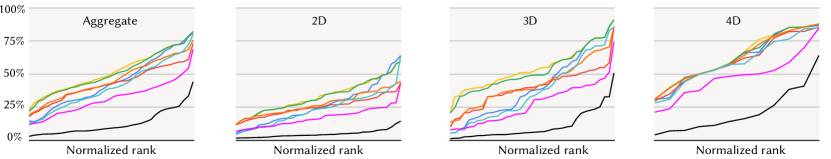
Figure 1: FP rates (vertical axis) for each test object, sorted in ascending order (horizontal axis). We show all methods (colored lines) across all dimensions (horizontal subplots). While Tbl. 1 reports average performance, this graphical representation reveals that our method OurNeural, despite having a few higher negative examples, consistently yields the lowest FP rates across all categories. In contrast, methods like AABox exhibit extremely variable performance, with select examples exceeding an 80 % FP rate.

Speed  This is the speed of the bounding operation itself (e.g. evaluating the closed-form sphere intersection, or, for method OurNeural, a network forward pass). We report both query speed and ray throughput as the average number over 500 independent runs with 10 million randomly sampled, forward-facing 3D rays. For fairness, our methods and all baselines have been implemented as vectorized PyTorch code and make full use of GPU acceleration.

4.4 Results

Quality  We show our quantitative results and the comparisons against the baselines in Tbl. 1. As is evident, our method OurNeural consistently outperforms the other baselines by a large margin (up to 8$\times$ improvement on 4D point queries). The second-best methods are on average kDOP and OurkDOP, sometimes roughly on-par with AABox. Interestingly, using modern gradient-descent based construction for OurkDOP improves on kDOP results significantly. Unsurprisingly, all methods increase their FP rate when going to higher dimension, a testimony to the increased query complexity. Notably, our method scales favorably with dimension and achieves acceptable FP rates even at high dimensions (e.g. for 4D box queries). Interestingly, looking at the relative intra-dimensional performance of our method reveals that it performs almost consistently worst on plane queries, which leaves room for future research and improvement. Moreover, especially in higher dimensions (e.g. 4D ray, plane, box), the baselines approach near uniform performance, differing by only a few percentage points. We attribute this to their rigidity: the rotating object carves out the same amount of space, and any rigid fit to this time-varying volume will perform almost equally poorly. Fig. 1 visualizes the same data in the form of a rank plot, see figure caption for discussion. Qualitative results for 2D and 3D are shown and discussed in Fig. Neural Bounding and Fig. 2, respectively.

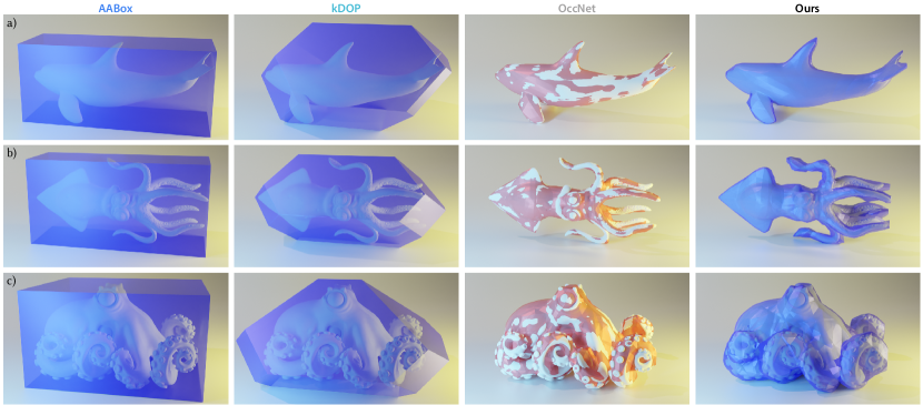
Figure 2: Comparison of methods (columns) for different 3D shapes (rows). AABox and kDOP both bound the objects conservatively, but create false positives, whereas OccNet bounds overtight and produces false negatives (red). Our approach is both tight and conservative.

Fig. 5 shows our OurNeural for NNs of different complexity. Fig. 6 shows a bounding hierarchy on a school of 2D fish.

Figure 3: Result for OurkDOP.

In Fig. 3 we show result for OurkDOP, $k=6$: the resulting parameters are compatible with any $k$-DOP implementation and as fast to test. The only difference is that the planes were found via stochastic gradient descent (using Adam) and our loss. Ours performs better than the common heuristics [Eri04]. This indicates that our approach to finding bounding parameters can be superior to heuristics, even if the model itself is not neural.

Figure 4: Conservative bounding of never-hit (blue) and always-hit (yellow).

We further show a result for an interesting variant of our method, that does not conservatively state which spatial location might be hit, but conservatively bounds which spatial locations certainly are hit. This is achieved by flipping the asymmetry-weights $\alpha$ and $\beta$ . An example is seen in Fig. 4 for 2D and Fig. 9 in 3D. This is useful for a quick broad-phase test in collision: an object only needs to be tested if it is neither certainly out nor certainly-in.

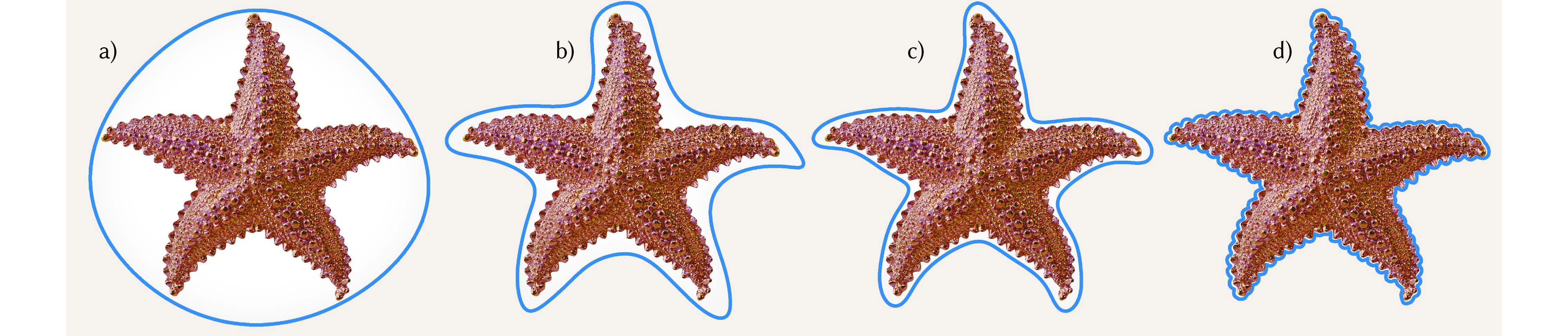
Figure 5: Our learned bounding volumes with increasingly complex neural networks from left to right. A simple network, left, fits the shape only roughly, but still conservative. With increasing expressiveness towards the right, the fit gets more accurate and recovers concave regions, and later, the curvature of the starfish’s arms. For a complex NN it becomes almost pixel-exact, but even then, small approximation errors are made but never violating the bounding requirement (zero FN). This indicates we can guarantee conservativeness independent of complexity.

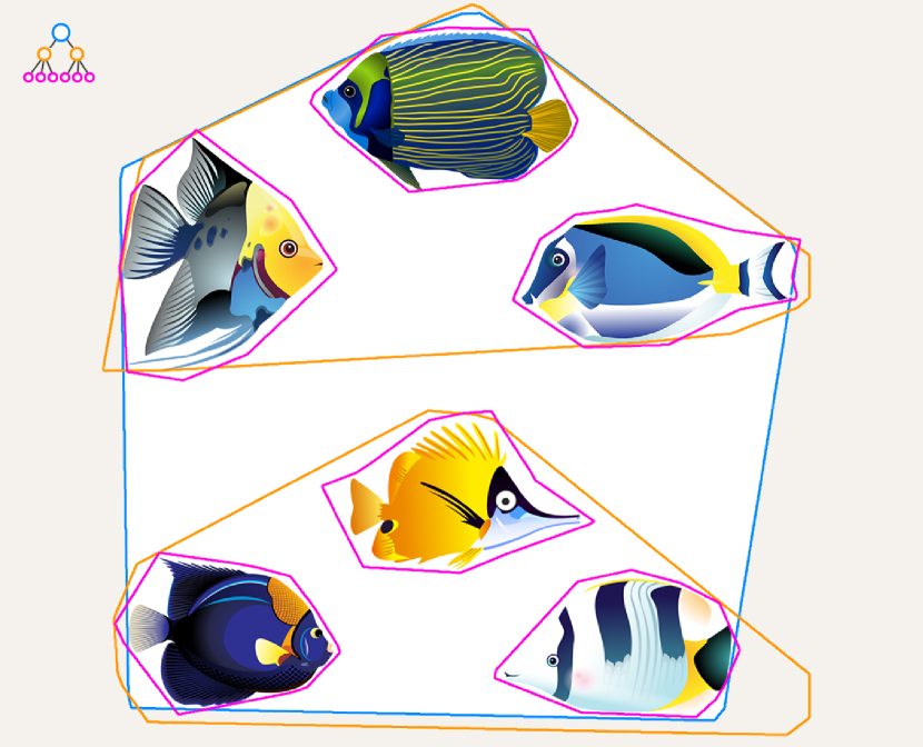
Figure 6: A hierarchy of neural bounding networks. The first level is show in blue, the two child nodes in yellow and the leafs in pink. Note that it is not required for the higher-level bounding to bound the lower-level boundings. It is only required to bound the indicator.

Speed  We quantify the speed of our bounding operations in Tbl. 2. While we obviously cannot match the speed of simpler bounding methods such as Sphere or AABox, we were surprised to find that our implementation of our neural bounding queries is only marginally slower than kDOP and some of the oriented bounding methods. We attribute this to the fact that inverting the bounding primitive’s orientation, which is necessary for oriented boundings in order to test against their simpler axis-aligned counterparts, already requires one matrix multiplication, whereas our network architecture only requires three in total. Therefore, even if we nominally lag behind in this comparison (by a factor of max. 2.5$\times$, OurNeural vs AAElli), we would argue that this is offset by the the substantial reduction in FP that our method achieves (see Tbl. 1, on average our method incurs only 23.8 % of AAElli’s FPs, and Sec. 5).

Table 2: Speed and throughput of different methods. Throughput is reported in billions of rays per second. The last column shows the respective method’s DOF in indicator dimension $n$ .

	Speed (ms)	Throughput	DoF
AABox	0.028	35.98	2$n$
OBox	0.044	22.79	3$n$
Sphere	0.022	45.13	$n+1$
AAElli	0.020	49.50	2$n$
OElli	0.036	28.08	3$n$
kDOP	0.048	21.06	$k(n+1)$
OurkDOP	0.018	52.80	$k(n+1)$
OurNeural	0.050	19.90	50$n$

5 Discussion

Can a network that is slower than traditional bounding primitives be useful in practical graphics problems? There are two main supportive arguments we will discuss in the following: tightness and scalability.

Tightness  In order to evaluate the speed of a bounding method, one must additionally take into account the cost of a false-positive query, i.e. having to perform an intersection against the detailed, bounded geometry. Assume a bounding method B can be queried in time $t_{b}$, and the competing bounding method A is five times slower, i.e. $t_{a}=5\,t_{b}$. Assume further that A, in spite of being slower, produces significantly fewer false-positives ($p_{a}=0.1$) than B ($p_{b}=0.3$). The total time for $N$ tests, regardless of the method used, is $Nt_{i}+p_{i}\cdot N\cdot t$, of which the first term marks indispensable checks (as every ray must be checked against the bounding method), and the second term marks unnecessary checks due to false-positive bounding queries. Finally, assume that performing tests with the actual detailed geometry needs time $t$, which is usually much larger than $t_{a}$ and $t_{b}$. Hence, for method A to win, the following must hold:

N$$\cdot t_{a}+Np_{a}\cdot t <N\cdot t_{b}+Np_{b}\cdot t$$

$$t_{a}+p_{a}\cdot t <t_{b}+p_{b}\cdot t$$

$$t_{a}+p_{a}\cdot t-p_{b}\cdot t <t_{b}$$

$$p_{a}\cdot t-p_{b}\cdot t <t_{b}-t_{a}$$

$$t(p_{a}-p_{b}) <t_{b}-t_{a}$$

$$\textrm{and hence if }(p_{a}-p_{b})>0:\quad t <(t_{b}-t_{a})/(p_{a}-p_{b})$$

$$\textrm{or otherwise if }(p_{a}-p_{b})<0:\quad t >(t_{b}-t_{a})/(p_{a}-p_{b}).$$ (2)

For the aforementioned example values, this produces

$$t>(t_{b}-5\,t_{b})/(0.1-0.3)=20\,t_{b},$$

which means that method A is to be preferred if tests against the actual bounded geometry are at least 20 times as expensive as the bounding query. As traditional triangle meshes often have millions to billions of triangles, this is easily achieved by our approach.

We quantify the exact ratio of times a 3D ray-geometry test has to be more expensive than the bounding test in Tbl. 3 and see that, while with increasing number of rays the ratio rises, our method is on average to be preferred when the geometry test is as little as 2.43$\times$ more expensive than the bounding test, which certainly is achieved in most real-world applications.

Table 3: Times a test against the actual geometry has to be more expensive than the bounding test for our method to pay off, as per the previously developed inequality Eq. 2.

N	AABox	OBox	Sphere	AAElli	OElli	kDOP	OurkDOP
0.1 M	1.42	1.66	1.60	1.65	1.52	2.40	3.29
1.0 M	1.55	1.99	2.14	2.40	2.21	3.27	3.34
10.0 M	2.66	2.81	3.64	4.14	2.89	3.75	5.97

Scalability  From our results one can easily see that our method’s advantage increases with dimensionality. We visualize this in detail in Fig. 7. This is because in concave shapes of natural high-dimensional signals, empty space grows much quicker than is intuitive. High-dimensional space is mostly empty, but not always [AHK01]. This is also why NNs excel as classifiers and best imagined in four dimensions, space plus time, where the space-time indicator of a moving objects is highly concave but mostly empty, and well represented by a NN of low complexity: a bit of bending, and that is already much better than any box or sphere.

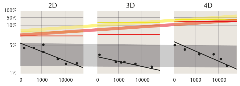
Figure 7: False positive rate in percentage (vertical axis) as a function of model complexity, i.e. number of tuned parameters (horizontal axis in each subplot) for three different dimensions (subplots). Different colors are different methods (OBox, Sphere, OurNeural; baselines are constants with respect to complexity which remains fixed in each dimension). Across dimensions, we see that FPs increase for baselines, while for ours, the rate (still function of model complexity itself) remains roughly constant (funnels).

To demonstrate scalability to complex high-dimensional spaces, we finally bound an entire generative model itself in Fig. 8. We use a pre-trained variational auto-encoder (VAE) of MNIST digits as the indicator. This is a 12-dimensional space, consisting of 10 latent dimensions of the VAE and two more dimensions that denote the pixel coordinate in the output image. Note that a pre-trained MNIST VAE is a deterministic 12-D indicator function like any other function in this paper, independent of the question how it was trained non-deterministic. This allows to predict which pixels will belong to a digit, without even running the generative model. While this is a toy problem, in more engineered applications it would, e.g. allow conservative ray intersection with complex 3D models that have not even yet been generated.

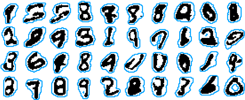
Figure 8: Results of applying our method to a VAE that generates MNIST digits, here shown for random latent codes. The blue borders are the conservative per-digit bounds produced by our method.

Limitations  However, our approach also comes with certain limitations, which we will highlight here to inspire future work:

As we overfit a network per shape, our approach requires additional storage in the order of magnitude of the network parameters (e.g. 2,951 parameters for a 3D point query network), which naturally is larger than for traditional baselines (see Tbl. 2). However, storage is cheaper than compute, and moreover, applications which use bounding geometry usually handle meshes with several million to trillion triangles. We therefore believe that our modest storage requirement for the network parameters is negligible in comparison.

Moreover, training one of our bounding networks takes significantly longer than inferring traditional bounding primitives, many of which have closed-form solutions. While this can easily be outsourced to a pre-processing stage, we do see further potential in maximizing training speed by either incorporating the fully-fused NN architecture proposed by [MESK22] into our approach, or by meta-learning [SCT^∗20, FR22, TMW^∗21] a space of bounding networks, which would be especially useful for bounding similar geometry that only slightly differs in shape or pose.

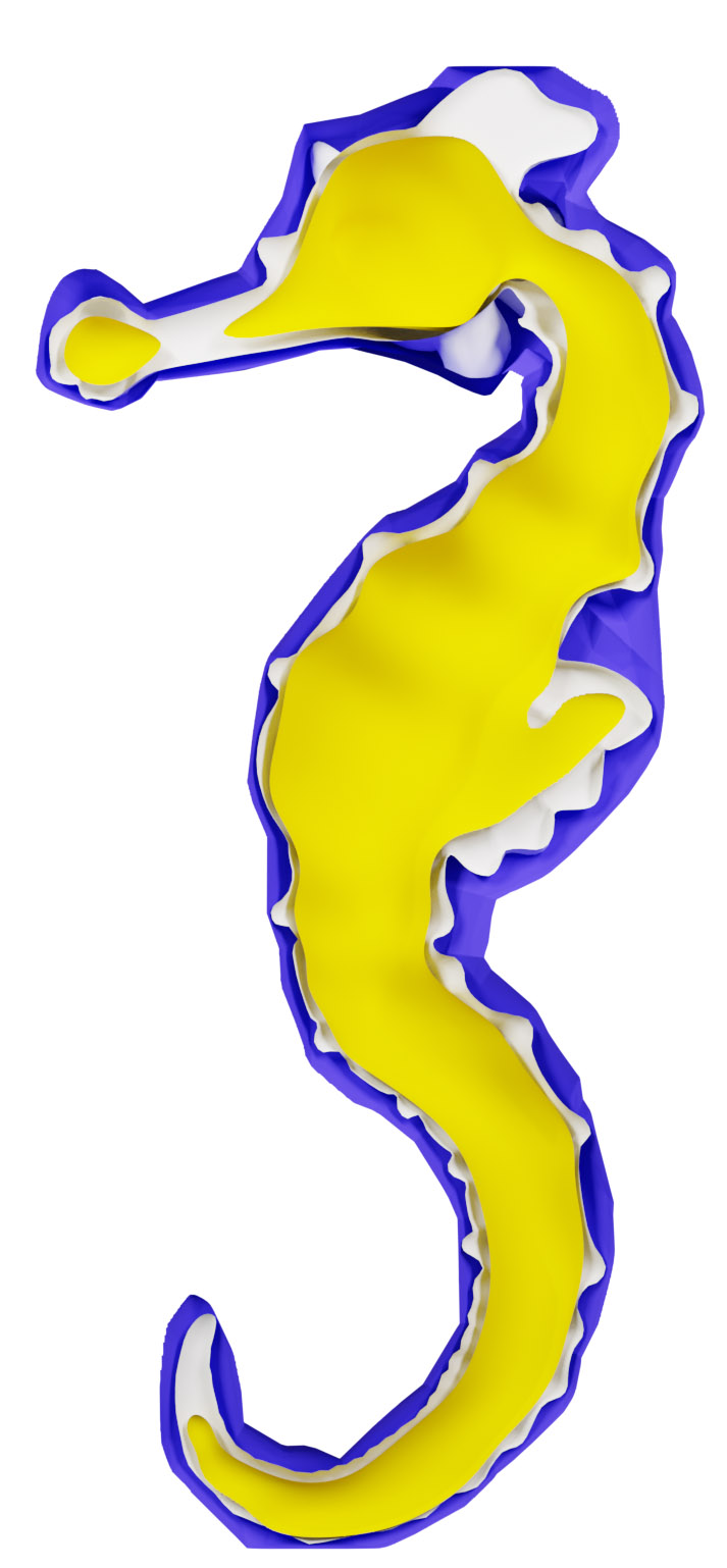
Figure 9: 3D-bounding no-hit (blue) and hit (yellow).

Our results are only almost always conservative, as they involve two stages of sampling, that, in expectation, will be conservative, but we lack any proof under what conditions the probability of being truly conservative is how high. The step of sampling the query region could be replaced by an unbiased (and potentially closed-form) one; we only choose sampling here as it works on any indicator in any dimension, However, the loss is still an empirical loss, and there is a nonzero chance that a tiny part of the indicator would remain unattended with finitely many samples. In practice, our results show dozens of tasks with dozens of instances, each tested with hundred-thousands of samples with no FN on any sample.

6 Conclusion

In future work, the idea of asymmetric losses might be applicable to other neural primitives like hashing. In a similar vein, distance fields could be trained to maybe underestimate, but never overestimate distance so as to aid sphere tracing. It is further conceivable to bound not only geometry but also other quantities like radiance fields or their statistics for image synthesis. While we train to not have FN, the same idea can be made conservative on the inverse indicator, so to have no FP. This would require a second network, which as a pair with the inverse conservatively forms a crust, or trust region. In terms of application, future work could study robot configurations, where a typical application to study with this proxy is collision-free path planning.

Using our technique, bounding in graphics can benefit from many of the exciting recent innovations around NNs such as improved architectures, advanced training, or dedicated neural hardware.

Appendix A Architecture

Tbl. 4 details the architectures used for all results in this paper.

Table 4: Architecture details for all results show in this paper.

Result	Ind.	Query	Network	PE
Fig. Neural Bounding	2D	Point	2$\times$20$\times$10$\times$5$\times$1	0
Tbl. 1	2D	Point	2$\times$25$\times$25$\times$1	0
Tbl. 1, Fig. 1	2D	Ray	4$\times$25$\times$25$\times$1	0
Tbl. 1, Fig. 1	2D	Plane	4$\times$25$\times$25$\times$1	0
Tbl. 1, Fig. 1	2D	Box	4$\times$25$\times$25$\times$1	0
Tbl. 1, Fig. 1	3D	Point	3$\times$50$\times$50$\times$1	0
Tbl. 1, Fig. 1	3D	Ray	6$\times$50$\times$50$\times$1	0
Tbl. 1, Fig. 1	3D	Plane	6$\times$50$\times$50$\times$1	0
Tbl. 1, Fig. 1	3D	Box	6$\times$50$\times$50$\times$1	0
Tbl. 1, Fig. 1	4D	Point	4$\times$75$\times$75$\times$1	0
Tbl. 1, Fig. 1	4D	Ray	8$\times$75$\times$75$\times$1	0
Tbl. 1, Fig. 1	4D	Plane	8$\times$75$\times$75$\times$75$\times$1	0
Tbl. 1, Fig. 1	4D	Box	8$\times$75$\times$75$\times$1	0
Tbl. 2	3D	Ray	6$\times$50$\times$50$\times$1	0
Fig. 2, a, b	3D	Point	3$\times$100$\times$100$\times$100$\times$1	0
Fig. 2, c	3D	Point	3$\times$50$\times$50$\times$1	0
Fig. 4	2D	Point	2$\times$10$\times$1	0
Fig. 5, a	2D	Point	2$\times$10$\times$10$\times$1	0
Fig. 5, b	2D	Point	2$\times$10$\times$10$\times$5$\times$1	0
Fig. 5, c	2D	Point	2$\times$25$\times$25$\times$5$\times$1	0
Fig. 5, d	2D	Point	2$\times$128$\times$128$\times$128$\times$1	18
Fig. 7, 2D	2D	Point	2$\times$$a$$\times$$a$$\times$1	0
Fig. 7, 3D	3D	Point	3$\times$$b$$\times$$b$$\times$1	0
Fig. 7, 4D	4D	Point	4$\times$$c$$\times$$c$$\times$1	0
Fig. 6	2D	Point	2$\times$25$\times$25$\times$1	0
Fig. 8	12D	Point	12$\times$25$\times$25$\times$1	0
Fig. 9, hit	3D	Point	3$\times$40$\times$40$\times$1	0
Fig. 9, no-hit	3D	Point	3$\times$100$\times$100$\times$100$\times$1	0

$a\in\{10,16,25,50,75,125\}$
$b\in\{25,50,64,75,125,256\}$
$c\in\{75,125,256,512,768,1024\}$

References

- [AHK01] Aggarwal C. C., Hinneburg A., Keim D. A.: On the surprising behavior of distance metrics in high dimensional space. In Database Theory (2001), pp. 420–434.
- [AL20] Atzmon M., Lipman Y.: Sal: Sign agnostic learning of shapes from raw data. In CVPR (2020), pp. 2565–2574.
- [Ber97] Bergen G. v. d.: Efficient collision detection of complex deformable models using AABB trees. J Graphics Tools 2, 4 (1997), 1–13.
- [BM23] Behera A. P., Mishra S.: Neural directional distance field object representation for uni-directional path-traced rendering. arXiv preprint arXiv:2306.16142 (2023).
- [CCJK22] Cai X., Coevoet E., Jacobson A., Kry P.: Active learning neural c-space signed distance fields for reduced deformable self-collision. In Graphics Interface (2022).
- [Dou92] Dougherty E. R.: An introduction to morphological image processing. In SPIE (1992).
- [EL01] Ehmann S. A., Lin M. C.: Accurate and fast proximity queries between polyhedra using convex surface decomposition. Comp Graph Forum 20, 3 (2001), 500–511.
- [Eri04] Ericson C.: Real-time collision detection. Crc Press, 2004.
- [FKH23] Fujieda S., Kao C.-C., Harada T.: Neural intersection function. arXiv preprint arXiv:2306.07191 (2023).
- [FR22] Fischer M., Ritschel T.: Metappearance: Meta-learning for visual appearance reproduction. ACM Trans Graph (Proc. SIGGRPAH) 41, 6 (2022), 1–13.
- [GHFB13] Gu Y., He Y., Fatahalian K., Blelloch G.: Efficient BVH construction via approximate agglomerative clustering. In Proc. HPG (2013), pp. 81–88.
- [GPSS07] Gunther J., Popov S., Seidel H.-P., Slusallek P.: Realtime ray tracing on GPU with BVH-based packet traversal. In Symp Interactive Ray Tracing (2007), pp. 113–118.
- [HNN23] Hashimoto K., Naito T., Naito H.: Neural polytopes. arXiv preprint arXiv:2307.00721 (2023).
- [HZRS16] He K., Zhang X., Ren S., Sun J.: Deep residual learning for image recognition. In CVPR (2016), pp. 770–778.
- [IS15] Ioffe S., Szegedy C.: Batch normalization: Accelerating deep network training by reducing internal covariate shift. In ICCV (2015), pp. 448–456.
- [KB14] Kingma D. P., Ba J.: Adam: A method for stochastic optimization. arXiv preprint arXiv:1412.6980 (2014).
- [KHM∗98] Klosowski J. T., Held M., Mitchell J. S., Sowizral H., Zikan K.: Efficient collision detection using bounding volume hierarchies of -DOPs. IEEE TVCG 4, 1 (1998), 21–36.
- [KK86] Kay T. L., Kajiya J. T.: Ray tracing complex scenes. ACM SIGGRAPH Computer Graphics 20, 4 (1986), 269–278.
- [KRWM22] Karnewar A., Ritschel T., Wang O., Mitra N.: ReLU fields: The little non-linearity that could. In ACM SIGGRAPH (2022), pp. 1–9.
- [LFR23] Liu C., Fischer M., Ritschel T.: Learning to learn and sample BRDFs. Comp Graph Forum (Proc. Eurographics) 42, 2 (2023), 201–211.
- [MESK22] Müller T., Evans A., Schied C., Keller A.: Instant neural graphics primitives with a multiresolution hash encoding. ACM Trans Graph (Proc. SIGGRAPH) 41, 4 (2022), 1–15.
- [MOB∗21] Meister D., Ogaki S., Benthin C., Doyle M. J., Guthe M., Bittner J.: A survey on bounding volume hierarchies for ray tracing. Comp Graph Forum 40, 2 (2021), 683–712.
- [MON∗19] Mescheder L., Oechsle M., Niemeyer M., Nowozin S., Geiger A.: Occupancy networks: Learning 3d reconstruction in function space. In CVPR (2019).
- [NDS∗23] Nsampi N. E., Djeacoumar A., Seidel H.-P., Ritschel T., Leimkühler T.: Neural field convolutions by repeated differentiation. arXiv preprint arXiv:2304.01834 (2023).
- [PFS∗19] Park J. J., Florence P., Straub J., Newcombe R., Lovegrove S.: DeepSDF: Learning continuous signed distance functions for shape representation. In CVPR (June 2019).
- [PGM∗19] Paszke A., Gross S., Massa F., Lerer A., Bradbury J., Chanan G., Killeen T., Lin Z., Gimelshein N., Antiga L., et al.: Pytorch: An imperative style, high-performance deep learning library. NeurIPS 32 (2019).
- [RBBZ∗21] Ridnik T., Ben-Baruch E., Zamir N., Noy A., Friedman I., Protter M., Zelnik-Manor L.: Asymmetric loss for multi-label classification. In ICCV (2021), pp. 82–91.
- [RFB15] Ronneberger O., Fischer P., Brox T.: U-net: Convolutional networks for biomedical image segmentation. In Proc. MICCAI (2015), pp. 234–241.
- [RPLG21] Reiser C., Peng S., Liao Y., Geiger A.: Kilonerf: Speeding up neural radiance fields with thousands of tiny MLPs. In ICCV (2021), pp. 14335–14345.
- [SCT∗20] Sitzmann V., Chan E., Tucker R., Snavely N., Wetzstein G.: MetaSDF: Meta-learning signed distance functions. NeurIPS 33 (2020), 10136–10147.
- [SE02] Schneider P., Eberly D. H.: Geometric tools for computer graphics. Elsevier, 2002.
- [SJ22] Sharp N., Jacobson A.: Spelunking the deep: Guaranteed queries on general neural implicit surfaces via range analysis. ACM Trans Graph (Proc. SIGGRAPH) 41, 4 (2022), 1–16.
- [SOTC22] Santesteban I., Otaduy M., Thuerey N., Casas D.: Ulnef: Untangled layered neural fields for mix-and-match virtual try-on. NeurIPS 35 (2022), 12110–12125.
- [TMW∗21] Tancik M., Mildenhall B., Wang T., Schmidt D., Srinivasan P. P., Barron J. T., Ng R.: Learned initializations for optimizing coordinate-based neural representations. In CVPR (2021), pp. 2846–2855.
- [VRM∗18] Vogels T., Rousselle F., McWilliams B., Röthlin G., Harvill A., Adler D., Meyer M., Novák J.: Denoising with kernel prediction and asymmetric loss functions. ACM Trans Graph (Proc. SIGGRAPH) 37, 4 (2018), 1–15.
- [WMS∗14] Weller R., Mainzer D., Srinivas A., Teschner M., Zachmann G.: Massively parallel batch neural gas for bounding volume hierarchy construction. In VRIPHYS (2014), pp. 9–17.
- [XTS∗22] Xie Y., Takikawa T., Saito S., Litany O., Yan S., Khan N., Tombari F., Tompkin J., Sitzmann V., Sridhar S.: Neural fields in visual computing and beyond. Comp Graph Forum 41, 2 (2022).
- [YGKL21] Yariv L., Gu J., Kasten Y., Lipman Y.: Volume rendering of neural implicit surfaces. NeurIPS 34 (2021), 4805–4815.
- [ZLJ∗21] Zhou X., Liu X., Jiang J., Gao X., Ji X.: Asymmetric loss functions for learning with noisy labels. In ICML (2021), pp. 12846–12856.
- [ZWX∗22] Zesch R. S., Witemeyer B. R., Xiong Z., Levin D. I., Sueda S.: Neural collision detection for deformable objects. arXiv preprint arXiv:2202.02309 (2022).