Inverse Factorized Q-Learning for Cooperative Multi-agent Imitation Learning

Abstract.

This paper concerns imitation learning (IL) (i.e, the problem of learning to mimic expert behaviors from demonstrations) in cooperative multi-agent systems. The learning problem under consideration poses several challenges, characterized by high-dimensional state and action spaces and intricate inter-agent dependencies. In a single-agent setting, IL has proven to be done efficiently through an inverse soft-Q learning process given expert demonstrations. However, extending this framework to a multi-agent context introduces the need to simultaneously learn both local value functions to capture local observations and individual actions, and a joint value function for exploiting centralized learning. In this work, we introduce a novel multi-agent IL algorithm designed to address these challenges. Our approach enables the centralized learning by leveraging mixing networks to aggregate decentralized Q functions. A main advantage of this approach is that the weights of the mixing networks can be trained using information derived from global states. We further establish conditions for the mixing networks under which the multi-agent objective function exhibits convexity within the Q function space. We present extensive experiments conducted on some challenging competitive and cooperative multi-agent game environments, including an advanced version of the Star-Craft multi-agent challenge (i.e., SMACv2), which demonstrates the effectiveness of our proposed algorithm compared to existing state-of-the-art multi-agent IL algorithms.

1. Introduction

Imitation learning (IL) is a powerful approach for sequential decision making in complex high-dimensional environments in which agents can learn desirable behavior by imitating an expert. There is a wide range of applications of IL in several real-world domains, including healthcare Wang et al. (2020); Shah et al. (2022) and autonomous driving Zhou et al. (2021); Hawke et al. (2020); Le Mero et al. (2022). A rich body of literature on IL focuses on simple single-agent settings Abbeel and Ng (2004); Ho and Ermon (2016); Fu et al. (2017); Ziebart et al. (2008); Ross and Bagnell (2010); Garg et al. (2021). Existing approaches on this line of work are, however, not directly suitable for multi-agent settings due the interactive nature of multiple agents, making the environment non-stationary to individual agents. Recently, researchers develop new multi-agent imitation learning methods that are tailored to either cooperative or non-cooperative (or both) settings Song et al. (2018); Yu et al. (2019); Le et al. (2017); Bhattacharyya et al. (2018); Jeon et al. (2020); Šošić et al. (2016).

Among these existing multi-agent IL works, leading methods Song et al. (2018); Yu et al. (2019) explore equilibrium solution concepts for Markov games including Nash Hu et al. (1998) and logistic stochastic best response Yu et al. (2019). Findings on underlying properties of these solution concepts are then incorporated into extending the single-agent imitation learning models for multi-agent settings. While these multi-agent IL methods shows promising results on some cooperative and competitive multi-agent tasks, they still face difficulties in training in practice, which is the result of the underlying adversarial optimization process inherent from original single-agent IL methods Ho and Ermon (2016); Fu et al. (2017). Indeed, this adversarial optimization involves biased and high variance gradient estimators, leading to a highly unstable learning process.

Our work studies IL in cooperative multi-agent settings. We leverage recent advanced findings in both single-agent IL and cooperative multi-agent reinforcement learning (MARL) to build a unified multi-agent IL algorithm, named Multi-agent Inverse Factorized Q-learning (MIFQ). Essentially, MIFQ is built upon inverse soft Q-learning (IQ-Learn) Garg et al. (2021) — a leading single-agent IL method of which advantage is to learn a single Q-function that implicitly defines both reward and policy functions, thus avoiding adversarial training. To adapt inverse soft Q-learning for multi-agent settings, we then employ value-function factorization with mixing networks to model both the reward and state-value functions involves in the learning objective, inspired by the leading cooperative MARL method, QMIX Rashid et al. (2020). That is, individual state-value $V$-function and reward $R$-function of the agents are combined via two different mixing networks into joint $V$-values and $R$-values, which are then incorporated into the learning objective. This novel integration enables training decentralised imitation policies for agents in a centralised fashion, following the well-known paradigm of centralised training with decentralised execution in cooperative MARL Oliehoek et al. (2008); Kraemer and Banerjee (2016).

An important research question arising from this integration is that whether the objective function in multi-agent inverse soft Q-learning is still convex or not given the complication of mixing networks involved together with the value-function factorization. We remark that this convexity property is important as it guarantees the optimization objective is well-behaved and has an unique optimization solution, leading to the effectiveness of original single-agent IL method, IQ-Learn Garg et al. (2021). As our second contribution, we provide new theoretical results, showing that the objective remains convex in local Q-values of the agents when the mixing networks are convex and non-decreasing in the corresponding local state and reward values. Following with this theoretical finding, we show that using hyper-networks (that take global states as input and then output weights for mixing networks) with the commonly-used general two-layer neural network structures Rashid et al. (2020) will guarantee the convexity of the learning objective within the Q-function space.

Finally, we conduct extensive experiments in various multi-agent domains, including: SMACv2 Ellis et al. (2022), Gold Miner FPT (2020), and MPE (Multi Particle Environments) Lowe et al. (2017). We show that our algorithm MIFQ outperforms other baseline algorithms in all these environments. It is important to note that our experiments with SMACv2 mark the first time imitation learning algorithms are employed and evaluated on such a challenging multi-agent environment.

2. Related Work

Single-Agent Imitation Learning. There is a rich body of existing works focusing on generating policies that mimic an expert’s behavior given data of expert demonstrations in single-agent settings. A classic approach is behavioral cloning which casts IL as a supervised learning problem, attempting to maximize the likelihood of the expert’s trajectories Ross and Bagnell (2010); Pomerleau (1991). This approach, while simple, requires a large amount of data to work well due to its compounding error issue. An alternative approach is to recover the reward function (either implicitly or explicitly) for which the expert’s policy is optimal Fu et al. (2017); Ho and Ermon (2016); Reddy et al. (2019); Kostrikov et al. (2019); Finn et al. (2016). Leading methods Ho and Ermon (2016); Fu et al. (2017) follow an adversarial optimization process (which is similar to GAN Goodfellow et al. (2014)) to train the imitation policy and reward function alternatively. These adversarial training-based methods, however, suffer instability. A more recent work by Garg et al. (2021) overcomes this instability issue by introducing an inverse soft-Q learning process, i.e., learning a single Q-function from which corresponding policy and reward functions can be inferred. For a comprehensive review of literature on this topic, we refer readers to the survey article in Arora and Doshi (2021).

Multi-Agent Imitation Learning. Most of single-agent IL works, however, do not apply directly to multi-agent settings, mainly due to the non-stationarity of multi-agent environments. Literature on multi-agent IL is rather limited. A few works study multi-agent IL either in cooperative environments Barrett et al. (2017); Le et al. (2017); Šošić et al. (2016); Bogert and Doshi (2014) or competitive environments Lin et al. (2014); Reddy et al. (2012); Song et al. (2018); Yu et al. (2019). Recent leading methods employ equilibrium solution concepts in Markov games such as Nash equilibrium to extend some existing IL methods to the multi-agent settings Song et al. (2018); Yu et al. (2019). However, these methods still suffer the instability challenge during training as they still rely on adversarial training. Our work focuses on multi-agent IL in a fully cooperative Dec-POMDP environment. We utilize the idea of inverse soft-Q learning in single-agent IL Garg et al. (2021) to avoid adversarial training. We extend this idea to the multi-agent settings under the paradigm of centralized learning decentralized execution from MARL, allowing an efficient and stable learning process. It is worth noting that Bui et al. (2023) also develops an inverse soft Q-learning procedure for enhancing a PPO-based MARL algorithm. Their IL method differs from our algorithm, as it is designed specifically for the situation that actions are missing in the demonstrations, and only focuses on decentralized learning.

Multi-Agent Reinforcement Learning (MARL). The literature of MARL encompasses a number of advanced methods, including both centralized and decentralized algorithms. While centralized algorithms (Claus and Boutilier, 1998) focus on learning a unified joint policy that governs the collective actions of all agents, decentralized learning, pioneered by (Littman, 1994), involves optimizing each agent’s local policy independently. Additionally, there exists a category of algorithms known as centralized training and decentralized execution (CTDE). For instance, methods detailed in Lowe et al. (2017) and Foerster et al. (2018) employ actor-critic architectures and train a centralized critic that takes global information into account. Value-decomposition (VD) methods (Sunehag et al., 2017; Rashid et al., 2020), represent the joint Q-function as a function of agents’ local Q-functions. QMIX, as introduced by (Rashid et al., 2020), offers a more advanced VD method for consolidating agents’ individual local Q-functions through the utilization of mixing and hyper-network (Ha et al., 2017) concepts. There are also other policy gradient based MARL algorithms. For instance, (de Witt et al., 2020) develops independent PPO (IPPO), a decentralized MARL, that can achieve high success rates in several hard SMAC maps. (Yu et al., 2022) develops MAPPO, a PPO version for MARL that achieves SOTA results on several tasks, and recently, Bui et al. (2023) proposes IMAX-PPO, an enhanced PPO algorithm for MARL. Our work utilizes MAPPO to train our expert and generate expert demonstrations. We also employ a hyper-network architecture (Ha et al., 2017) to facilitate centralized learning, following a similar approach in (Rashid et al., 2020).

3. Preliminaries

3.1. Cooperative Multi-agent Reinforcement Learning (Coop-MARL)

A multi-agent cooperative system can be described as a decentralized partially observable Markov decision process (Dec-POMDP), defined by a tuple $\{{\mathcal{S}},{\mathcal{O}},{\mathcal{N}},{\mathcal{A}},P,R\}$ Oliehoek et al. (2016), where ${\mathcal{S}}$ is the set of global states shared by all the agents, ${\mathcal{O}}$ is the set of local observations of agents, and ${\mathcal{N}}$ is all the agents. In addition, ${\mathcal{A}}=\prod_{i\in{\mathcal{N}}_{\mathcal{A}}}{\mathcal{A}}_{i}$ is the set of joint actions of all the agents, ${\mathcal{A}}_{i}$ is the set of actions of an agent $i\in{\mathcal{N}}$, and $P$ is the transition dynamics of the multi-agent environment. Finally, in Coop-MARL, all agents share the same reward function, $R$, that can take inputs as global states and actions of all the agents and return the corresponding rewards.

At each time step where the global state is $S$, each ally agent $i\in{\mathcal{N}}$ takes an action $a_{i}\in{\mathcal{A}}_{i}$ according to a policy $\pi_{i}(a_{i}\mid o_{i})$, where $o_{i}$ is the local observation of agent $i$. The joint action is defined as $A=\{a_{i}\mid i\in{\mathcal{N}}\}$ and the joint policy is defined accordingly:

$$\Pi(A\mid S)=\prod\nolimits_{i\in{\mathcal{N}}}\pi_{i}(a_{i}\mid o_{i}).$$

After all the agent actions are executed, the global state is updated to a new state $S^{\prime}\in{\mathcal{S}}$ with the transition probability $P(S^{\prime}\mid A,S)$. The objective of the Coop-MARL problem is to find a joint policy $\Pi(\cdot\mid S)=\prod_{i}\pi_{i}(\cdot\mid o_{i})$ that maximizes the expected long-term joint reward, formulated as follows:

$$\max\limits_{\Pi}\mathbb{E}_{\Pi}\Big{[}\sum\limits_{t=0}^{\infty}R(A_{t},S_{t})\Big{]}$$

3.2. Imitation Learning

In imitation learning (IL), the objective is to recover an expert reward or expert policy function from some expert demonstration data. Several IL methods were developed for single-agent settings Abbeel and Ng (2004); Ho and Ermon (2016); Fu et al. (2017); Ziebart et al. (2008); Ross and Bagnell (2010); Garg et al. (2021). In general, we can directly extend these methods to a fully-observable cooperative multi-agent setting by considering global states and joint actions of the agents in a similar fashion as in the single-agent settings. Let’s denote a set of expert demonstrations as ${\mathcal{D}}^{E}=\{\tau=\{(A_{t},S_{t}),\leavevmode\nobreak\ t=0,1...\}\}$ where $A_{t}$ is the joint action of all agents and $S_{t}$ is the global state at time step $t$. In the following, we describe some popular IL approaches accordingly.

3.2.1. Behavioral Cloning

A classical approach for imitation learning is Behavioral Cloning (BC), where the objective is to maximize the likelihood of the demonstrations:

$$\max_{\Pi}\sum_{\tau\in{\mathcal{D}}^{E}}\sum_{t}\ln\big{(}\Pi(A_{t}\mid S_{t})\big{)}$$

It is commonly known that BC has a strong theoretical foundation, as it can guarantee to return the exact expert policy. However, BC ignores the environment’s dynamics and only works well with offline learning. As a result, it often requires a huge number of samples to achieve a desired performance Ross et al. (2011).

3.2.2. Distribution Matching

State-of-the-art (SOTA) IL algorithms are typically based on distribution matching. Specifically, let $\rho^{\Pi}(S,A)$ be the occupancy measure of visiting the state $S$ and joint action $A$, under the joint policy $\Pi$, defined as follows:

$$\rho^{\Pi}(S,A)=\Pi(S\mid A)\prod_{t=0}^{\infty}\gamma^{t}P(S_{t}=S\mid\Pi)$$

The objective is to minimize a divergence between the occupancy measure of the learning policy $\rho^{\Pi}$ and that of the expert’s policy $\rho^{\Pi^{E}}$. For instance, the imitation learning can be done by solving:

$$\min_{\Pi}\Big{\{}\textsc{KL}\left(\rho^{\Pi}\Big{\|}\rho^{\Pi^{E}}\right)\Big{\}}=\min_{\Pi}\mathbb{E}_{(S,A)\sim\rho^{\Pi}}\Big{[}\ln\frac{\rho^{\Pi^{E}}(S,A)}{\rho^{\Pi}(S,A)}\Big{]}$$

IL algorithms based on distributional matching include some SOTA IL methods such as adversarial IL (Ho and Ermon, 2016; Fu et al., 2017) or IQ-Learn (Garg et al., 2021).

4. Multi-agent Inverse Q-Learning

As mentioned previously, our new algorithm is built upon an integration of recent advanced findings in imitation learning (i.e., the new leading IL algorithm IQ-Learn Garg et al. (2021)) and in multi-agent reinforcement learning (i.e., the SOTA algorithm QMIX Rashid et al. (2020)). In the following, we first present the main idea of IQ-Learn, with some direct centralized and decentralized adaptations to multi-agent settings. We then discuss key shortcomings of such simple adaptations in the context of a Dec-POMDP environment. Finally, we present our new algorithm which tackles all those shortcomings.

4.1. Inverse Soft Q-Learning

4.1.1. Centralized Inverse Q-Learning

In a fully-observable cooperative multi-agent setting, single-agent IL algorithms including IQ-Learn can be directly applied by using global states and joint actions of the agents in a similar fashion as in single-agent settings. Given demonstration samples ${\mathcal{D}}^{E}=\{\tau=\{(A_{t},S_{t}),\leavevmode\nobreak\ t=0,1...\}\}$ where $A_{t}$ is the joint action and $S_{t}$ is the global state at step $t$, the goal of IQ-Learn is to solve the following maximin problem, which is also the objective of adversarial learning-based IL approaches Ho and Ermon (2016); Fu et al. (2017):

$$\max\limits_{R}\min\limits_{\Pi}\Big{\{}L(R,\Pi) =\mathbb{E}_{(S,A)\sim\rho^{E}}\big{[}R(S,A)\big{]}$$

$$-\mathbb{E}_{\rho^{\Pi}}\big{[}R(S,A)\big{]}-\mathbb{E}_{\rho^{\Pi}}\big{[}\ln\Pi(S,A)\big{]}\Big{\}}$$ (1)

where $\rho^{E}$ is the occupancy measure given by the expert policy $\pi^{E}$ and $\mathbb{E}_{\rho^{\Pi}}\big{[}\ln\Pi(S,A)\big{]}$ is the entropy regularizer. A typical approach to solve this maximin problem is to run an adversarial optimization process over rewards and policies, of which idea is similar to generative adversarial networks Ho and Ermon (2016); Fu et al. (2017). However, such an approach suffers instability, a well-known challenge of adversarial training.

In a more recent work (Garg et al., 2021), Garg et al. introduce a new IL algorithm, IQ-Learn, which avoids adversarial training by learning a single soft Q-function, of which definition is provided below.

Definition (Soft Q-function Garg et al. (2021)).

For a reward function R and a policy $\Pi$, the soft Bellman operator ${\mathcal{B}}^{\Pi}$ is defined as:

$$({\mathcal{B}}^{\Pi}Q)(S,A)=R(S,A)+\gamma\mathbb{E}_{S^{\prime}\sim P(\cdot\mid S,A)}V^{\Pi}(S^{\prime})$$

where $V^{\Pi}(S)=\mathbb{E}_{A\sim\Pi(\cdot\mid S)}\big{[}Q(S,A)-\log\Pi(A\mid S)\big{]}$. The soft Bellman operator is contractive and defines a unique soft Q-function for the reward function $R$, given as $Q={\mathcal{B}}^{\Pi}Q$.

Essentially, Garg et al. show that the above maximin problem is equivalent to the following single minimization problem which only requires optimizing over the soft Q-function:

$$\min\nolimits_{Q}\Big{\{}J(Q) =\mathbb{E}_{(S,A)\sim\rho^{E}}\Big{[}\gamma\mathbb{E}_{S^{\prime}\sim P(\cdot\mid S,A)}\big{[}V^{Q}(S^{\prime})\big{]}-Q(S,A)\Big{]}$$

$$\qquad+(1-\gamma)\mathbb{E}_{S^{0}}\big{[}V^{Q}(S^{0})\big{]}\Big{\}}$$ (2)

where $Q:{\mathcal{S}}\times{\mathcal{A}}\rightarrow\mathbb{R}$ is the soft Q-function and $S^{0}$ is the initial state. Importantly, the loss functions $J(Q)$ is shown to be convex in $Q$, making the IQ-Learn advantageous to use (Garg et al., 2021).

Given $Q$, the optimal policy can be computed accordingly (Garg et al., 2021):

$$\Pi^{Q}(A\mid S)=\frac{1}{Z_{S}}\exp(Q(S,A))$$

where $Z_{S}$ is the normalization factor. Finally, the state-value $V^{Q}(S)$, $S\in{\mathcal{S}}$ can be computed as follows:

$$V^{Q}(S)=V^{\Pi^{Q}}(S)=\ln\Big{(}\sum\nolimits_{A}\exp(Q(S,A))\Big{)}$$

A shortcoming of the above centralized IQ-Learn approach is that it not scalable in complex multi-agent settings since the joint action space grows exponentially in the number of agents. Furthermore, it requires full observations for agents, which is not applicable in a Dec-POMDP environment with only local partial observations.

4.1.2. Independent Inverse Q-Learning

An alternative approach to overcome the shortcomings of centralized IQ-Learn is to consider a separate IL problem for each individual agent, taking into account local observations of that agent. Specifically, one can set the objective to recover a local Q function $Q_{i}(a_{i}\mid o_{i})$, as a function of a local observation $o_{i}$ and local action $a_{i}$, for each agent $i\in{\mathcal{N}}$. The local IQ-Learn loss function can be formulated as follows:

$$\min\nolimits_{Q_{i}}\Big{\{}J_{i}(Q_{i}) =\mathbb{E}_{(o_{i},a_{i})\sim{\mathcal{D}}^{E}}\Big{[}\gamma\mathbb{E}_{o^{\prime}_{i}\sim P(\cdot\mid S,A)}\big{[}V^{Q}_{i}(o^{\prime}_{i})\big{]}-Q_{i}(o_{i},a_{i})\Big{]}$$

$$\qquad+(1-\gamma)\mathbb{E}_{o^{0}_{i}}\big{[}V^{Q}_{i}(o^{0}_{i})\big{]}\Big{\}}$$ (3)

where $V^{Q}_{i}(o_{i})=\ln\Big{(}\sum_{a_{i}\in{\mathcal{A}}_{i}}\exp\big{(}Q(o_{i},a_{i})\big{)}\Big{)}$. Here, $o^{\prime}_{i}\sim P(\cdot\mid S,A)$ is equivalent to $o^{\prime}_{i}$ is the local observation of agent $i$ corresponding to the new state $S^{\prime}\sim P(\cdot\mid S,A)$.

Let $Q^{*}_{i}(o_{i},a_{i})$ be an output of the training $\min_{Q_{i}}J_{i}(Q_{i})$, then a local reward and policy function can be recovered (Garg et al., 2021) as follows:

$$r^{*}(o_{i},a_{i}) =Q^{*}_{i}(o_{i},a_{i})-\gamma\mathbb{E}_{o^{\prime}_{i}\sim P(\cdot|S,A)}[V_{i}^{Q^{*}}(o^{\prime}_{i})]$$ (4)

$$\pi^{*}_{i}(a_{i}\mid o_{i}) =\frac{\exp(Q^{*}_{i}(o_{i},a_{i}))}{\sum_{a^{\prime}_{i}\in{\mathcal{A}}_{i}}\exp(Q^{*}(o_{i},a^{\prime}_{i}))}$$

Let us denote $r^{Q}_{i}(o_{i},a_{i})=Q_{i}(o_{i},a_{i})-\gamma\mathbb{E}_{o^{\prime}_{i}\sim P(\cdot\mid S,A)}\big{[}V^{Q}_{i}(o^{\prime}_{i})\big{]}$, then the objective in (3) can be rewritten as follows:

$$\min\nolimits_{Q_{i}}\!\Big{\{}J_{i}(Q_{i}) =\mathbb{E}_{(o_{i},a_{i})\sim{\mathcal{D}}^{E}}\big{[}\!-r^{Q}_{i}(o_{i},a_{i})\big{]}+(1-\gamma)\mathbb{E}_{o^{0}_{i}}\big{[}V^{Q}_{i}(o^{0}_{i})\big{]}\Big{\}}$$ (5)

Thus, independent IQ-Learn can be understood as the process of reconstructing a local reward function, denoted as $r^{Q}_{i}$ for each agent $i$, with the objective of minimizing the negation of the expected reward generated by the expert’s policy. We will leverage this insight to build mixing networks that facilitate centralized learning.

Overall, this approach enables decentralized policies for agents, allowing it to work in a Dec-POMDP environment. However, it faces the challenge of instability due to the non-stationarity of the multi-agent environment. In addition, it does not leverage additional information on global states available during the training process.

4.2. Inverse Factorized Soft Q-Learning with Mixing Networks

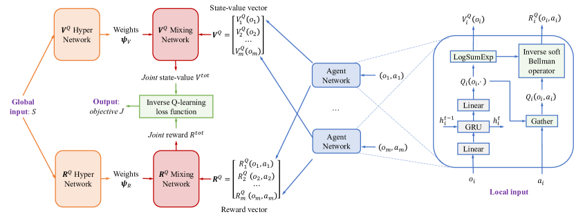
Figure 1. An overview of our multi-agent imitation learning architecture.

We now present our new multi-agent IL approach to learn decentralized value function $Q_{i}(o_{i},a_{i})$ in a centralized way. An overview of our approach is illustrated in Figure 4. Our key idea involves creating (i) agent local Q-value networks that output local Q-values $Q(o_{i},a_{i})$ given local information $(o_{i},a_{i})$ of each agent $i$; and (ii) mixing networks that utilize global information such as global states to combine local values of agents into joint values used to compute the objective of the inverse soft Q-learning. In addition, we employ hyper-networks that provide a rich representation for the weights of the mixing networks, allowing us to govern their value ranges.

4.2.1. Multi-agent IL Network Architecture

Overall, our network architecture comprises of three different types of networks:

Agent local $Q$-value networks.

To start, let us define $\textbf{Q}(S,A)$ as a vector $\textbf{Q}(S,A)=\big{[}Q_{1}(o_{1},a_{1}),Q_{2}(o_{2},a_{2}),\cdots,Q_{m}(o_{m},a_{m})\big{]}$ of local soft Q-values of agents where $m=|{\mathcal{N}}|$ is the number of agents and $(o_{i},a_{i})\in(S,A),\leavevmode\nobreak\ i\in{\mathcal{N}}$. For an abuse of notations, we also denote by $Q_{i}(o_{i},a_{i};\theta_{i})$ as the local $Q$-value network of the agent $i$ of which learnable parameter is $\theta_{i}$. Each local Q-value network takes an input as a pair $(o_{i},a_{i})$ of a local observation and an action of agent $i$ and then output the corresponding local soft $Q$-value $Q_{i}(o_{i},a_{i})=Q_{i}(o_{i},a_{i};\theta_{i})$.

We then use this vector $\textbf{Q}(S,A)$ to compute the corresponding state-value vector $\textbf{V}^{Q}(S)=\big{[}V^{Q}_{1}(o_{1}),V^{Q}_{2}(o_{2}),\cdots,V^{Q}_{m}(o_{m})\big{]}$ as described in Section  4.1, formulated as follows:

$$V^{Q}_{i}(o_{i})=\ln\Big{(}\sum\nolimits_{a_{i}}\exp\big{(}Q_{i}(o_{i},a_{i})\big{)}\Big{)}$$

In addition, let $\textbf{R}^{Q}(S,A)=\big{[}r^{Q}_{1}(o_{1},a_{1}),r^{Q}_{2}(o_{2},a_{2}),\cdots,r^{Q}_{m}(o_{m},a_{m})\big{]}$ as a reward vector comprising of local rewards $r^{Q}_{i}(o_{i},a_{i})$ of all agents $i$ where $i\in{\mathcal{N}}$. This reward vector can be computed using the inverse soft Bellman operator as follows:

$$\textbf{R}^{Q}(S,A)=\textbf{Q}(S,A)-\gamma\mathbb{E}_{S^{\prime}\sim P(\cdot\mid S,A)}\big{[}\textbf{V}^{Q}(S)\big{]}$$

The values of $\textbf{V}^{Q}$ and $\textbf{R}^{Q}$ will be passed to the corresponding mixing networks to induce the joint state and reward values $V^{tot}$ and $R^{tot}$ respectively. These two joint values will be then incorporated into computing the objective of the inverse soft Q-learning.

State-value and reward mixing networks.

We create two different mixing networks to combine local state values $\textbf{V}^{Q}$ and local reward values $\textbf{R}^{Q}$ into joint values $V^{tot}$ and $R^{tot}$, respectively. Let’s denote these mixing networks as ${\mathcal{M}}_{\psi_{V}}(\cdot)$ and ${\mathcal{M}}_{\psi_{R}}(\cdot)$. Here $\psi_{V}$ and $\psi_{R}$ are corresponding weights (or parameters) of these two mixing networks. In particular, we have:

$$V^{tot}(S)={\mathcal{M}}_{\psi_{V}}\big{(}\textbf{V}^{Q}(S)\big{)}$$

$$R^{tot}(S,A)={\mathcal{M}}_{\psi_{R}}\big{(}-\textbf{R}^{Q}(S,A)\big{)}$$

We can now formulate the objective function of our multi-agent inverse factorized Q-learning with respect to the local $Q$-values and these mixing networks, as follows:

$$\min_{\textbf{Q}}\Big{\{} J(\textbf{Q},\psi_{R},\psi_{V})=\!\!\!\!\!\!\sum_{(S,A)\in{\mathcal{D}}^{E}}\!\!\!\!\!\!\!R^{tot}(S,A)+(1-\gamma)\mathbb{E}_{S^{0}}\big{[}V^{tot}(S_{0})\big{]}\Big{\}}$$ (6)

Hyper-networks.

Finally, we create two hyper-networks corresponding the two mixing networks. These hyper-networks take the global state $S$ as an input and generate the weights $\psi_{V}$ and $\psi_{R}$ of the mixing networks accordingly. The creation of such hyper-networks allows us to have a rich representation of the weights that can be governed to ensure the convexity of the objective $J(\textbf{Q},\psi_{R},\psi_{V})$ in the local $Q$-values $\textbf{Q}(S,A)$ (as we show next). We can write $\psi_{V}=\psi_{V}(S;\omega_{V})$ and $\psi_{R}=\psi_{R}(S;\omega_{R})$ where $\omega_{V}$ and $\omega_{R}$ denote trainable parameters of the state-value and reward hyper-networks.

In the end, we can alternatively write the objective function $J(\textbf{Q},\psi_{R},\psi_{V})$ as $J(\theta,\omega_{R},\omega_{V})$ when the local soft $Q$-values Q are parameterized by $\theta=\{\theta_{1},\theta_{2},\cdots,\theta_{m}\}$ and the weights of the mixing networks $(\psi_{V},\psi_{R})$ are parameterized by $\omega_{V}$ and $\omega_{R}$ respectively. We note that we will use either $J(\textbf{Q},\psi_{R},\psi_{V})$ or $J(\theta,\omega_{R},\omega_{V})$ depending on the context of our analysis.

4.2.2. Convexity of Multi-Agent IL Objective Function

One of key properties that make original IQ-Learn advantageous in single-agent settings is that its loss function is convex in $Q$. Therefore, we aim at exploring conditions under which the loss function in (6) is convex in Q in our case. For the sake of representation, we will use a common notation X which represents either $\textbf{V}^{Q}(S)$ or $-\textbf{R}^{Q}(S,A)$, depending on whether we are referring to the state-value mixing network ${\mathcal{M}}_{\psi_{V}}(\cdot)$ or reward mixing network ${\mathcal{M}}_{\psi_{R}}(\cdot)$, respectively. [Convexity] Suppose ${\mathcal{M}}_{\psi_{V}}(\textbf{X})$ and ${\mathcal{M}}_{\psi_{Q}}(\textbf{X})$ are convex in X, non-decreasing in each element $X_{i}$, then the objective function $J(\textbf{Q},\psi_{R},\psi_{V})$ is convex in Q . The results in Theorem 3 are general, in the sense that, as shown below, any feed-forward mixing networks with non-negative weights and nonlinear convex activation functions will satisfy the assumption in Theorem (3), implying the convexity of $J(\textbf{Q},\cdot,\cdot)$. Any feed-forward mixing networks ${\mathcal{M}}_{\psi_{R}}(\textbf{X})$ and ${\mathcal{M}}_{\psi_{V}}(\textbf{X})$ constructed with non-negative weights and nonlinear non-decreasing convex activation functions (such as ReLU or ELU or Maxout) are convex and non-decreasing in X. As a result, Corollary 4.2.2 below states that a commonly used two-layers feed-forward network with non-negative weights and convex activation functions will satisfy the conditions in Theorem 3 and help preserve the convexity of $J(\textbf{Q})$.

Corollary (Convexity under two-layer feed-forward mixing networks)

Suppose the mixing networks ${\mathcal{M}}_{\psi_{R}}(\textbf{X}),{\mathcal{M}}_{\psi_{V}}(\textbf{X})$ are two-layer feed-forward neural networks of the form $\sigma(\textbf{X}\times|W_{1}|+b_{1})\times|W_{2}|+b_{2}$ where $W_{1},W_{2},b_{1},b_{2}$ are weight and bias vectors of appropriate sizes and $\sigma$ are some nonlinear convex and non-increasing activation functions (such as ReLU or eLU or Maxout), then $J(\textbf{Q},\psi_{R},\psi_{V})$ is convex in Q.

The network structure mentioned in Corollary 4.2.2 consists of two layers with convex activation functions. It also requires that the weights of every layer are non-negative. Such two-layer mixing structure is widely used in prior MARL works Rashid et al. (2020). Furthermore, as shown in Theorem 3, the convexity of $J(\textbf{Q},\psi_{R},\psi_{V})$ still holds under multi-layer feed-forward mixing networks, as long as the activation functions are convex and the weights of each layer are non-negative. We note that the two-layer structure in Corollary 4.2.2 is sufficient for the mixing network to approximate any monotonic function arbitrarily closely in the limit of infinite width Dugas et al. (2009).

4.2.3. Relation with Independent Inverse Q-Learning.

In its simplest form, mixing networks can be expressed as merely a linear combination of local networks $Q_{i}$. We show that in this special case, our inverse factorized soft Q-Learning is equivalent to independent inverse Q-learning. In particular, if the mixing networks are constructed as weighted sums of $Q_{i}$ with non-negative weights, it can be demonstrated that minimizing $J(\textbf{Q},\psi_{R},\psi_{V})$ is essentially equivalent to minimizing each individual local $J_{i}(Q_{i})$ (Proposition 4.2.3). One advantage of this linear combination is that it ensures the decentralized objective functions fully align with their centralized counterparts. However, a drawback is the disregard for centralized learning and inter-agent dependencies. Despite this drawback, it underscores the important connection between decentralized and centralized learning. To achieve this, it suffices to have mixing networks ${\mathcal{M}}_{\psi_{R}}(\cdot)$ and ${\mathcal{M}}_{\psi_{V}}(\cdot)$ monotonically increasing. With this condition met, for two reward functions $\textbf{R}^{Q}=(r^{Q}_{i},\leavevmode\nobreak\ i\in{\mathcal{N}})$ and $\textbf{R}^{Q^{\prime}}=(r^{Q^{\prime}}_{i},\leavevmode\nobreak\ i\in{\mathcal{N}})$ such that $r^{Q}_{i}\geq r^{Q^{\prime}}_{i}$ for any $i\in{\mathcal{N}}$, we then can see that ${\mathcal{M}}_{\psi_{R}}\big{(}-\textbf{R}^{Q}(S,A)\big{)}\leq{\mathcal{M}}_{\psi_{R}}\big{(}-\textbf{R}^{Q^{\prime}}(S,A)\big{)}$. As a result, the monotonicity ensures that an increase in $r^{Q}_{i}$ will result in both a decrease in the local objective $J^{i}(Q_{i})$ and the global objective $J(\textbf{Q},\psi_{R},\psi_{V})$. Note that, to achieve monotonicity, it suffices to ensure that all the weights of the mixing networks non-negative.

Proposition (Linear combination)

If ${\mathcal{M}}_{\psi_{R}}(\textbf{X})$ and ${\mathcal{M}}_{\psi_{V}}(\textbf{X})$ are weighted sums of $X_{i}$ with non-negative weighting parameters, i.e., ${\mathcal{M}}_{\psi_{R}}(\textbf{X})={\mathcal{M}}_{\psi_{V}}(\textbf{X})=\sum_{i}\alpha_{i}X_{i}$, $\alpha_{i}\geq 0$ ($\forall i\in{\mathcal{N}}$), then $J(\textbf{Q},\psi_{R},\psi_{V})$ is convex in Q. Moreover, minimizing $J(\textbf{Q},\psi_{R},\psi_{V})$ over the Q space is equivalent to minimizing each local loss function $J_{i}(Q_{i})$. That is,

$$\operatorname*{argmin}\limits_{\textbf{Q}}\big{\{}J(\textbf{Q},\psi_{R},\psi_{V})\big{\}}=\big{[}\operatorname*{argmin}\limits_{Q_{1}}J_{1}(Q_{1}),\cdots,\operatorname*{argmin}\limits_{Q_{m}}J_{m}(Q_{m})\big{]}$$

4.3. Practical MIFQ Algorithm

We now present our practical multi-agent IL algorithm, MIFQ, together with details of our implemented network architecture.

1 Input: Environment $ENV$, parameters $\theta=(\theta_{1},\ldots,\theta_{m})$ and $(\omega_{R},\omega_{V})$, expert’s demonstrations ${\mathcal{D}}^{E}$, policy replay buffer $D^{replay}=\emptyset$, and learning rates $\lambda_{\theta}$ and $\lambda_{\omega}$.

2 while a certain number of loops do

3       $ENV.reset()$;

4       $\#$ Collect samples for replay buffer

5       for a certain number of collecting steps do

6             Execute policies $\pi_{i}\!=\!\text{softmax}\leavevmode\nobreak\ \leavevmode\nobreak\ Q_{i}(o_{i},a_{i}\!\mid\!\theta_{i}),\leavevmode\nobreak\ \forall i\!\in\!{\mathcal{N}}$ in the environment $ENV$ to collect new transition samples $\{(S,A,S^{\prime})\}$ and add them to ${\mathcal{D}}^{replay}$;

7      

8      $\#$ Run gradient descent with mini-batches $\sim{\mathcal{D}}^{replay}$

9       for a certain number of training steps do

10             Set $\theta\leftarrow\theta-\lambda_{\theta}\nabla_{\theta}J(\theta,\omega_{R},\omega_{V})$;

11             Set $(\omega_{R},\omega_{V})\leftarrow(\omega_{R},\omega_{V})\!-\!\lambda_{\omega}\!\nabla_{\omega_{R},\omega_{V}}J(\theta,\omega_{R},\omega_{V})$;

12            

13      

14$\#$ Recover agent policies and rewards

$$\text{Local policies: }\pi_{i}(a_{i}|o_{i}) =\frac{\exp(Q_{i}(o_{i},a_{i},\theta_{i}))}{\sum_{a^{\prime}_{i}\in{\mathcal{A}}_{i}}\exp(Q_{i}(o_{i},a^{\prime}_{i},\theta_{i}))},\leavevmode\nobreak\ \leavevmode\nobreak\ \forall i\in{\mathcal{N}};$$

$$\text{Local rewards: }r_{i}(o_{i},a_{i}) =Q_{i}(o_{i},a_{i})-\gamma\mathbb{E}_{o^{\prime}_{i}\sim P(\cdot|S,A)}[V_{i}^{Q}(o^{\prime}_{i})];$$

Algorithm 1 Multi-agent Inverse Factorized Q-Learning

4.3.1. Mixing and Hyper Networks

We employ the following two-layer feed-forward network structure for our two main mixing networks ${\mathcal{M}}_{\psi_{R}}(\textbf{X})$ and ${\mathcal{M}}_{\psi_{V}}(\textbf{X})$:

$${\mathcal{M}}_{\psi_{R}}(\textbf{X}) =\textsc{ELU}(\textbf{X}\times|W^{R}_{1}|+b^{R}_{1})\times|W^{R}_{2}|+b^{R}_{2}$$ (7)

$${\mathcal{M}}_{\psi_{V}}(\textbf{X}) =\textsc{ELU}(\textbf{X}\times|W^{V}_{1}|+b^{V}_{1})\times|W^{V}_{2}|+b^{V}_{2}$$ (8)

where $\psi_{R}=\{W^{R}_{1},W^{R}_{2},b^{R}_{1},b^{R}_{2},\}$ and $\psi_{V}=\{W^{V}_{1},W^{V}_{2},b^{V}_{1},b^{V}_{2}\}$ are the weight and bias vectors of the mixing networks. The absolute operations $|\cdot|$ are employed to ensure that all the weights are non-negative and, ensuring the convexity of the loss function and the alignment between centralized and local Q functions. Moreover, $\psi_{R}$ and $\psi_{V}$ are an output of a hyper-network taking the global state $S$ as input. Each hyper-network consists of two fully-connected layers with a ReLU activation. The output of each hyper-network is a vector, which is then reshaped into a matrix of appropriate size to be used in the corresponding mixing network. Finally, ELU is employed in the mixing networks to mitigate the problem of gradient vanishing and to ensure that negative inputs remain negative (not being zeroed out as in ReLU). Indeed, ELU is convex and the two mixing networks ${\mathcal{M}}_{\psi_{R}}$ and ${\mathcal{M}}_{\psi_{V}}$ follow the network structure stated in Corollary 4.2.2, implying that the loss function $J(\textbf{Q},\psi_{R},\psi_{V})$ is convex in Q and monotonically increasing in each local $Q_{i}$. The mixing structure in (7) and (8) is similar to those employed in QMIX (Rashid et al., 2020).

4.3.2. MIFQ: Multi-agent Inverse Factorized Q-Learning Algorithm

This section presents a practical implementation of our algorithm. Similar to Garg et al. (2021), we use a $\chi^{2}$-regularizer $\phi(x)=x+\frac{1}{2}x^{2}$ for the first terms of the loss function in (6). This convex regularizer is useful to ensure that that the term $\phi(R^{tot}(S,A))$ is lower-bounded even when the reward values go to $-\infty$, which is crucial to keep the learning process stable. In addition, similar to Garg et al. (2021), instead of directly estimating $\mathbb{E}_{S_{0}}{[V^{tot}(S_{0})]}$, we utilize the following equation to approximate $\mathbb{E}_{S_{0}}{[V^{tot}(S_{0})]}$ which can stabilize training:

$$(1-\gamma)\mathbb{E}[V(S)]=\mathbb{E}_{(S,A)\sim\rho}\big{[}V(S)-\gamma\mathbb{E}_{S^{\prime}\sim P(\cdot|S,A)}[V(S^{\prime})]\big{]}$$

for any value function $V(\cdot)$ and occupancy measure $\rho$ (Garg et al., 2021), we can estimate $\mathbb{E}_{S_{0}}{[V^{tot}(S_{0})]}$ by sampling $(S,A)$ from replay buffer and estimate $\mathbb{E}_{(S,A,S^{\prime})\sim\text{replay}}[V^{tot}(S)-\gamma V^{tot}(S^{\prime})]$ instead. In summary, we will employ the following practical loss function:

$$\min_{\theta,\omega_{R},\omega_{V}}\Big{\{} J(\theta,\omega_{R},\omega_{V})=\sum\nolimits_{(S,A)\in{\mathcal{D}}^{E}}\phi\big{(}R^{tot}(S,A)\big{)}$$

$$\quad+\mathbb{E}_{(S,A,S^{\prime})\in{\mathcal{D}}^{replay}}\big{[}V^{tot}(S)-\gamma V^{tot}(S^{\prime})\big{]}\Big{\}}$$ (9)

where $\theta=(\theta_{1},...,\theta_{m})$ are the training parameters of the $Q_{i}$ networks, and $\omega_{R}$ and $\omega_{V}$ are the parameters of the hyper-networks. The main steps of our MIFQ algorithm are shown in Algorithm 1.

4.3.3. Continuous Action Space

The formulations and algorithm presented above are unsuitable for continuous action spaces because the values of $V^{Q}_{i}$ in (3) may not be explicitly computed w.r.t an infinite number of actions. Therefore, we discuss in the following, an algorithm to handle this continuous-action situation. Essentially, we consider the following maximin problem, adapted from the actor-critic implementation of the single-agent IQ-Learn Garg et al. (2021):

$$\max_{\Pi}\min_{\textbf{Q}}\Big{\{} J(\textbf{Q},\Pi)=\!\!\!\!\!\sum_{(S,A)\in{\mathcal{D}}^{E}}\!\!\!\!\!\!R^{tot,\Pi}(S,A)+(1-\gamma)\mathbb{E}_{S^{0}}\big{[}V^{tot,\Pi}(S_{0})\big{]}\Big{\}}$$

This objective depends on an alternative estimation of the local state-value functions that is suitable for the continuous action space.

$$V^{\pi_{i}}_{i}(o_{i})=\mathbb{E}_{a_{i}\sim\pi_{i}(o_{i}\mid a_{i})}[Q_{i}(o_{i},a_{i})-\log\pi_{i}(a_{i}\mid o_{i})]$$

Given this alternative estimation, we can compute the local reward functions, and joint reward and state values accordingly:

$$\textbf{R}^{Q,\Pi}(S,A) =\textbf{Q}(S,A)-\gamma\mathbb{E}_{S^{\prime}\sim P(\cdot\mid S,A)}\big{[}\textbf{V}^{\Pi}(S)\big{]}$$

$$R^{tot,\Pi}(S,A) ={\mathcal{M}}_{\psi_{R}}(-\textbf{R}^{Q,\Pi}(S,A))$$

$$V^{tot,\Pi}(S) ={\mathcal{M}}_{\psi_{V}}(\textbf{V}^{\Pi}(S))$$

In other words, since the value function $V^{Q}$ and the agent policies $\pi^{Q}_{i}=\text{softmax}(Q_{i})$ cannot be explicitly computed as functions of $Q_{i}$, we can learn an additional policy function $\Pi=[\pi_{1},\ldots,\pi_{m}]$ and optimize it towards $\pi^{Q}_{i}$. This can be done by optimizing $J(\textbf{Q},\Pi)$ for any fixed $\Pi$, and for any fixed $(\textbf{Q},\psi_{R},\psi_{V})$, a soft actor-critic update can be done by solving the following optimization problem:

$$\max\nolimits_{\pi_{i}}\Big{\{}V^{\pi}_{i}(o_{i})=\mathbb{E}_{a_{i}\sim\pi_{i}(o_{i}\mid a_{i})}\big{[}Q_{i}(o_{i},a_{i})-\log\pi_{i}(a_{i}\mid o_{i})\big{]}\Big{\}}$$ (10)

which will bring $\pi_{i}$ closer to $\text{softmax}(Q_{i})$ (Garg et al., 2021). Moreover, the update in (10) will bring $V^{\pi}_{i}$ to higher values, thus making every element of $\textbf{R}^{Q,\Pi}$ and $\textbf{V}^{\Pi}$ larger. Moreover, the monotonicity of the mixing networks ${\mathcal{M}}_{\psi_{R}}$ and ${\mathcal{M}}_{\psi_{V}}$ then implies that such updates will also drive the values of $R^{tot,\Pi}(S,A)$ and $V^{tot,\Pi}(S)$ upward, thereby moving towards the goal of maximizing $J(\textbf{Q},\Pi)$ over $\Pi$.

5. Experiments

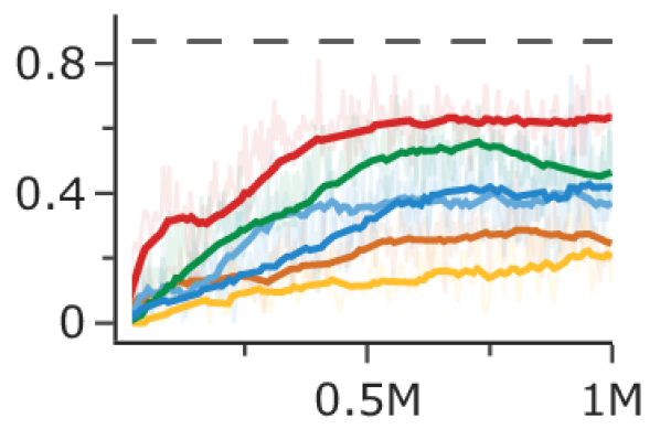
Figure 2. Convergence curves

protoss˙5˙vs˙5

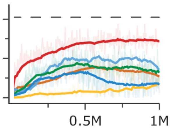
terran˙5˙vs˙5

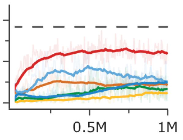
zerg˙5˙vs˙5

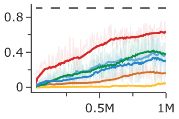
protoss˙10˙vs˙10

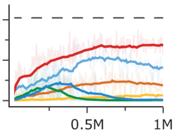
terran˙10˙vs˙10

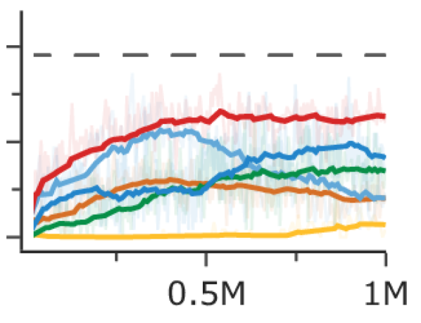
zerg˙10˙vs˙10

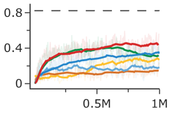
miner˙easy

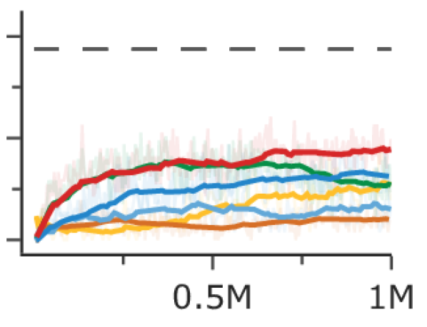
miner˙medium

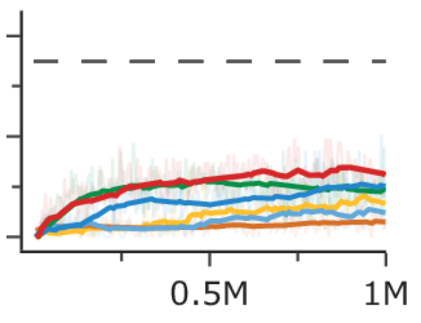
miner˙hard

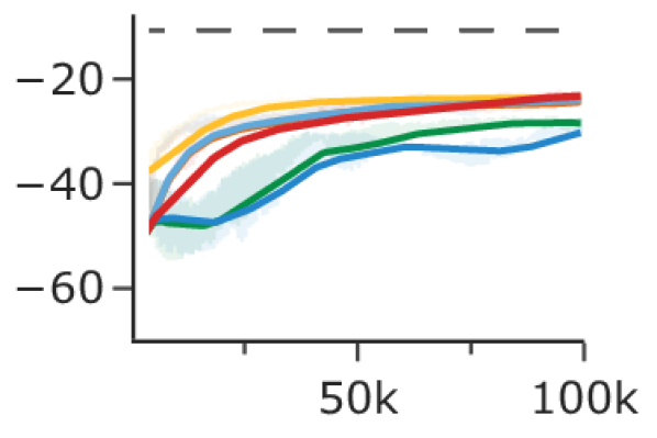
simple˙spread

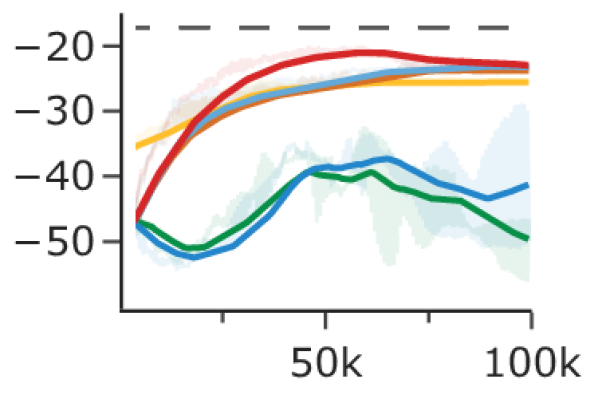
simple˙reference

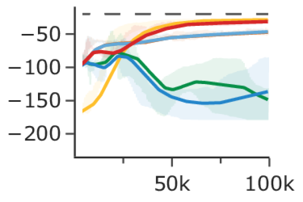
speaker˙listener

Table 1. Winrate and reward comparisons

Methods	Protoss		Terran		Zerg		Miner			MPE
	5vs5	10vs10	5vs5	10vs10	5vs5	10vs10	easy	medium	hard	reference	spread	speaker
Expert	87%	90%	82%	82%	74%	76%	82%	75%	70%	-17.2	-10.7	-19.7
BC	20%	5%	13%	5%	10%	5%	27%	22%	13%	-25.6	-23.6	-28.6
IIQ	25%	16%	22%	15%	17%	16%	15%	8%	6%	-23.8	-24.4	-47.3
IQVDN	37%	38%	29%	33%	21%	16%	18%	12%	10%	-23.2	-24.1	-46.6
MASQIL	46%	38%	25%	0%	13%	28%	32%	22%	18%	-49.6	-28.4	-148.5
MAGAIL	41%	30%	13%	1%	19%	33%	34%	25%	20%	-41.3	-30.3	-136.5
MIFQ (ours)	63%	62%	58%	54%	49%	51%	45%	36%	25%	-23.0	-23.3	-31.3

Figure 3. Comparison with different numbers of demonstrations. X-axis: winning rate. Y-axis: number of expert demonstrations.

SMACv2
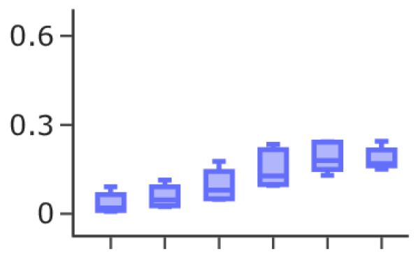
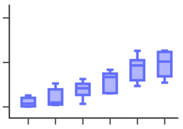
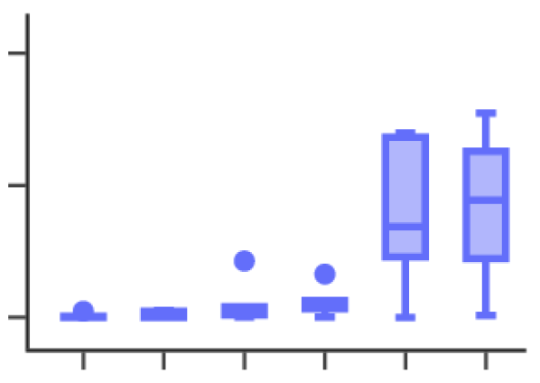
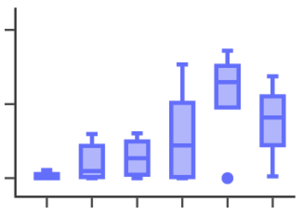
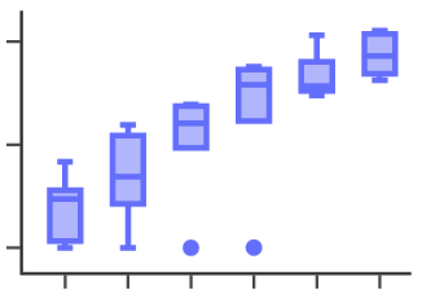
Gold Miner
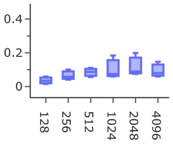
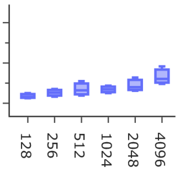
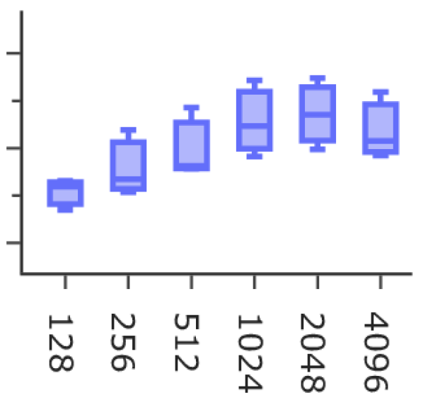
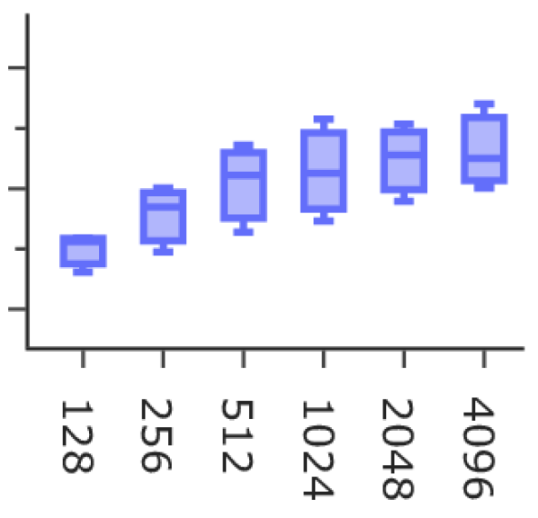
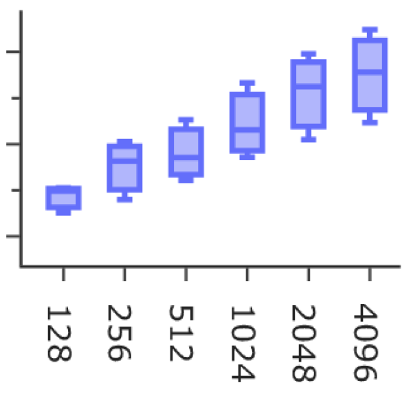
	IIQ	IQVDN	MASQIL	MAGAIL	MIFQ (ours)

5.1. Environments

We tested our algorithm on the following three environments.

5.1.1. SMACv2 Ellis et al. (2022)

SMAC is a well-known multi-agent environment based on the popular real-time strategy game named StarCraft II. In the game, players’ objective is to collect resources, erect structures, and assemble armies of units in order to defeat their enemies.

In SMAC, every unit is an autonomous agent whose actions rely solely on local observations constrained to a limited field of view centered around that specific unit. These groups of agents need to undergo training to effectively navigate complex combat scenarios, where they face off against an opposing army that is under the centralized command of the game’s pre-programmed AI.

SMAC has become a convenient environment for evaluating the effectiveness of MARL algorithms, providing challenging multi-agent settings with characteristics reflecting real-world scenarios, including partial observability, large numbers of agents, long-term planning, complex cooperative and competitive behaviors, etc.

We employ SMACv2 Ellis et al. (2022), an enhanced version of SMAC, that introduces a more formidable environment for evaluating cooperative MARL algorithms. In SMACv2, scenarios are procedurally generated, compelling agents to adapt to previously un-encountered situations during the evaluation phase. Comparing to SMACv1 Samvelyan et al. (2019), SMACv2 allows for randomized team compositions, diverse starting positions, and a heightened focus on promoting diversity. This benchmark comprises 6 sub-tasks, featuring a number of agents ranging from 5 to 10. These agents have the flexibility to engage with opponents of differing difficulty levels. Within the environment, there are allies playing against enemy players. Enemies’ policies are fixed and controlled by a simulator. We collect trajectories from well-trained ally agents and build IL to mimic them. The resulting imitating agents are then evaluated by letting them play against the simulator’s enemies.

5.1.2. Gold Miner FPT (2020)

This serves as another competitive multi-agent game, originating from a MARL competition. In this game, multiple miners navigate through a 2D terrain with obstacles and deposits of gold. Players earn points based on the amount of gold they successfully collect. There are two teams, ally and enemy, playing against each other. A victory is achieved when one team mined a larger average amount of gold than the other team. Winning this game is challenging since the agents must adapt to competing against exceptionally well-developed heuristic-based adversaries.

We consider three sub-tasks, each involves two ally agents against two enemy agents, sorted according to three difficulty levels: (i) Easy (easy_2_vs_2): The enemies employ a simple shortest-path strategy to reach the gold deposits; (ii) Medium (medium_2_vs_2): One enemy agent follows a greedy approach, while the other emulates the algorithm employed by the second-ranking team in the competition; and (iii) Hard (hard_2_vs_2): This the most challenging scenario, the enemy team consists of the first- and second-ranking teams from the competition. Finally, we collect demonstrations from well-trained allied agents playing against enemies of fixed policies controlled by a simulator. The resulting imitators are then evaluated by letting them play against the fixed enemies.

5.1.3. Multi Particle Environments (MPE) (Lowe et al., 2017)

MPE contains multiple communication-oriented deterministic multi-agent environments. We use three cooperative scenarios available in MPE for evaluating, including: (i) Simple_spread: three agents learn to avoid collisions while covering all of the landmarks; (ii) Simple_reference: two agents learn to get closer to the target landmarks. Each target landmark is known only by the other agents, so all agents have to communicate to each others; and (iii) Simple_speaker_listener: similar to simple_reference, but one agent (speaker) can speak, cannot move, and one agent (listener) can move, cannot speak.

5.2. Expert Demonstrations

For each task, we trained an expert policy by MAPPO algorithm with large-scale hyperparameters (multi layers, higher dimensions, longer training steps, more workers, using recurrent neural network, etc.). In term of expert buffer collection, we test each method with different numbers of expert trajectories: up to $128$ trajectories for MPEs and up to $4096$ trajectories for Miner and SMAC-v2. Note that MPEs are not dynamic environments, so we do not need a large number of expert demonstrations for evaluation. For each collected trajectory, we used a different random seed. After that, for a fair comparison, each method uses the same saved expert demonstrations for the training.

5.3. Baselines

We compare our MIFQ algorithm against other multi-agent IL algorithms, which either originate from the multi-agent IL literature, or be adapted from SOTA single-agent IL algorithms.

Behavior Cloning (BC). In a multi-agent setting, we can model each agent policy $\pi_{i}$ by a policy network and solving the maximum likelihood problem:

$$\max_{\pi_{i},i\in{\mathcal{N}}}\sum_{i\in{\mathcal{N}}}\sum_{(o_{i},a_{i})\in{\mathcal{D}}^{E}}\log\pi_{i}(a_{i}|o_{i}).$$

Independent IQ-Learn (IIQ). This is a straightforward adaption of IQ-Learn for a multi-agent setting, described in Section 4.1.2.

IQ-Learn with Value Decomposition Network (IQVDN). This is similar to our MIFQ algorithm, but instead of using mixing and hyper networks to aggregate agent Q functions, we employ the Value Decomposition (VDN) approach Sunehag et al. (2017).

MASQIL. This is our multi-agent adaption of SQIL (Reddy et al., 2019), a powerful framework to do imitation learning via RL. The idea is simply to assign a reward of 1 to any $(S,A)\in{\mathcal{D}}^{E}$, and 0 otherwise. IL then can be done by solving an RL problem with these new rewards. In our multi-agent setting, we adapt SQIL by employing the same reward assignment and utilize QMIX to recover policy functions. For a fair comparison, we apply the same mixing network architecture as in our MIFQ algorithm. As a result, MASQIL shares some similar advantages with our MIFQ, such as being non-adversarial and enabling decentralized learning through centralized learning.

MAGAIL. This is a multi-agent adversarial IL algorithm, developed by (Song et al., 2018). It is worth noting that alongside MAGAIL, there is another IL algorithm, MAAIRL (Yu et al., 2019). MAGAIL and MAAIRL share a similar adversarial structure and are competitive in performance. Therefore, it is necessary to only select one of them for comparison.

5.4. Comparison Results

We first train the imitation learning with different baselines, using 128 trajectories for MPE, and 4096 trajectories for SMACv2 and Miner. Figure 2 shows the evaluation scores of each methods comparing with expert scores on each tasks during training process. In comparison, we use the wining rate metric for SMACv2 & Gold Miner, and the reward score for MPEs, for visualization. Our method MIFQ outperforms SOTA multi-agent IL methods, i.e. MAGAIL and MAAIRL, on two hard tasks: SMACv2 & Gold Miner; and has competitive performance on MPEs. The details are shown in Table 1. Especially, on task protoss˙5˙vs˙5, our MIFQ reaches 63% of winning rate, higher than MAGAIL (41%) and MASQIL (46%), but it is still significantly lower than the expert level (87%). On other SMACv2 tasks, and even Gold Miner tasks, the performance gaps between IL methods and the experts are even higher. On the easiest tasks, MPEs, MIFQ has the best scores on simple˙reference and simple˙spread, but slightly worse than BC on speaker˙listener. Note that BC has a good performance for MPEs, which is not surprising as MPE is a deterministic environment.

To evaluate the efficiency of our method with different numbers of expert demonstrations/trajectories, we compare our MIFQ with MASQIL, MAGAIL, IQVDN and IIQ on two dynamic tasks: SMACv2 & Miner. With expert trajectories ranging from 128 to 4096, Figure 3 shows box and whisker plots of the average winning rate of each method on each task for data summarising analysis. As shown in the figure, our MIFQ method offers higher winrates, and it converges better with smaller standard errors. More details can be found in the appendix.

6. Conclusion

We developed a multi-agent IL algorithm based on the inversion of soft-Q functions. By employing mixing and hyper-network architectures, our algorithm, MIFQ, is non-adversarial and enables decentralized learning through a centralized learning approach. We demonstrated that, with some commonly used two-layer mixing network structures, our IL loss function is convex within the Q-function space, making learning convenient. Extensive experiments conducted across several challenging multi-agent tasks demonstrate the superiority of our algorithm compared to existing IL approaches. A potential limitation of MIFQ is that, while it achieves impressive performance across various tasks, it falls short of reaching the expertise levels. Furthermore, MIFQ, along with other baseline methods, struggles when confronted with very large-scale tasks, such as some of the largest game settings in SMACv2. Future work will focus on developing more sample-efficient and scalable IL algorithms to address these issues.

This research/project is supported by the National Research Foundation Singapore and DSO National Laboratories under the AI Singapore Programme (AISG Award No: AISG2-RP-2020-017). Dr. Nguyen was supported by grant W911NF-20-1-0344 from the US Army Research Office.

Appendix A Missing Proofs

A.1. Proof of Theorem 3

Theorem 3

Suppose ${\mathcal{M}}_{\psi_{V}}(\textbf{X})$ and ${\mathcal{M}}_{\psi_{Q}}(\textbf{X})$ are convex in X, non-decreasing in each element $X_{i}$, then the objective function $J(\textbf{Q},\psi_{V},\psi_{Q})$ is convex in Q .

Proof.

We first denote by Q as a vector comprising all the Q variables: $\textbf{Q}=\{Q_{i}(o_{i},a_{i}),\leavevmode\nobreak\ \forall o_{i},a_{i}\}$. To prove the main result, we will first verify the following lemmas:

Lemma

For any $i\in\ {\mathcal{N}}$,

$$V^{Q}_{i}(o_{i}) =\log\left(\sum_{a_{i}}\exp(Q_{i}(o_{i},a_{i}))\right)$$

$$-r^{Q}_{i}(o_{i},a_{i}) =-Q_{i}(o_{i},a_{i})+\gamma\mathbb{E}_{o^{\prime}_{i}\sim P(\cdot\mid S,A)}\big{[}V^{Q}_{i}(o^{\prime}_{i})\big{]}$$

are convex in Q.

Lemma

Let $\textbf{X}(\textbf{Q})=(X_{i}(\textbf{Q}),\ldots,X_{m}(\textbf{Q}))$ be a vector of size $m$ where each element is a convex function of Q, i.e., $X_{i}(\textbf{Q})$ is convex in Q for any $i\in{\mathcal{N}}$, ${\mathcal{M}}_{\psi_{R}}(\textbf{X}(\textbf{Q}))$ and ${\mathcal{M}}_{\psi_{V}}(\textbf{X}(\textbf{Q}))$ are convex in Q.

Lemma A.1 can be easily verified, as $V^{Q}_{i}(o_{i})$ has the log-sum-exp form, so it is convex in Q (Boyd and Vandenberghe, 2004). It follows that the term $\mathbb{E}_{o^{\prime}_{i}\sim P(\cdot\mid S,A)}\big{[}V^{Q}_{i}(o^{\prime}_{i})\big{]}$ is also convex in Q, implying the convexity of $-r^{Q}_{i}(o_{i},a_{i})$.

For Lemma A.1, we will make used general properties of convex function to verify the claim, i.e., we will prove that, for any two vector Q and $\textbf{Q}^{\prime}$, and any scalar $\alpha\in(0,1)$, the following inequality always holds

$$\alpha{\mathcal{M}}_{\psi_{R}}(\textbf{X}(\textbf{Q}))+(1-\alpha){\mathcal{M}}_{\psi_{R}}(\textbf{X}(\textbf{Q}^{\prime})) \geq{\mathcal{M}}_{\psi_{R}}(\textbf{X}(\alpha\textbf{Q}+(1-\alpha)\textbf{Q}^{\prime}))$$ (11)

$$\alpha{\mathcal{M}}_{\psi_{V}}(\textbf{X}(\textbf{Q}))+(1-\alpha){\mathcal{M}}_{\psi_{V}}(\textbf{X}(\textbf{Q}^{\prime})) \geq{\mathcal{M}}_{\psi_{V}}(\textbf{X}(\alpha\textbf{Q}+(1-\alpha)\textbf{Q}^{\prime}))$$

We will validate the inequality for ${\mathcal{M}}_{\psi_{R}}$; the same applies to ${\mathcal{M}}\psi_{V}$. According to the convexity of ${\mathcal{M}}_{\psi_{R}}(\textbf{X})$ in X, we can write

$$\alpha{\mathcal{M}}_{\psi_{R}}(\textbf{X}(\textbf{Q}))+(1-\alpha){\mathcal{M}}_{\psi_{R}}(\textbf{X}(\textbf{Q})) \geq{\mathcal{M}}_{\psi_{R}}(\alpha\textbf{X}(\textbf{Q})+(1-\alpha)\textbf{X}(\textbf{Q}^{\prime}))$$ (12)

$$={\mathcal{M}}_{\psi_{R}}\begin{pmatrix}\alpha X_{1}(\textbf{Q})+(1-\alpha)X_{1}(\textbf{Q}^{\prime})\\ \alpha X_{2}(\textbf{Q})+(1-\alpha)X_{2}(\textbf{Q}^{\prime})\\ ...\\ \alpha X_{m}(\textbf{Q})+(1-\alpha)X_{m}(\textbf{Q}^{\prime})\end{pmatrix}$$ (13)

Moreover, since $X_{i}(\textbf{Q})$ is convex in Q for all $i\in{\mathcal{N}}$, we have $\alpha X_{i}(\textbf{Q})+(1-\alpha)X_{i}(\textbf{Q}^{\prime})\geq X_{i}(\alpha\textbf{Q}+(1-\alpha)\textbf{Q}^{\prime})$. In addition, from the monotonicity of ${\mathcal{M}}_{\psi_{R}}(\textbf{X})$ in each element $X_{i}$, we have

$${\mathcal{M}}_{\psi_{R}}\begin{pmatrix}\alpha X_{1}(\textbf{Q})+(1-\alpha)X_{1}(\textbf{Q}^{\prime})\\ \alpha X_{2}(\textbf{Q})+(1-\alpha)X_{2}(\textbf{Q}^{\prime})\\ ...\\ \alpha X_{m}(\textbf{Q})+(1-\alpha)X_{m}(\textbf{Q}^{\prime})\end{pmatrix}\geq{\mathcal{M}}_{\psi_{R}}\begin{pmatrix}X_{1}(\alpha\textbf{Q}+(1-\alpha)\textbf{Q}^{\prime})\\ X_{2}(\alpha\textbf{Q}+(1-\alpha)\textbf{Q}^{\prime})\\ ...\\ X_{m}(\alpha\textbf{Q}+(1-\alpha)\textbf{Q}^{\prime})\end{pmatrix}={\mathcal{M}}_{\psi_{R}}(\textbf{X}(\alpha\textbf{Q}+(1-\alpha)\textbf{Q}^{\prime}))$$ (14)

Combine (13) and (14) we get

$$\alpha{\mathcal{M}}_{\psi_{R}}(\textbf{X}(\textbf{Q}))+(1-\alpha){\mathcal{M}}_{\psi_{R}}(\textbf{X}(\textbf{Q}))\geq{\mathcal{M}}_{\psi_{R}}(\textbf{X}(\alpha\textbf{Q}+(1-\alpha)\textbf{Q}^{\prime}))$$

which validates (11). We complete proving Lemma A.1.

We now go back to the main result. Considering ${\mathcal{M}}_{\psi_{R}}(-\textbf{R}^{Q}(S,A))$, we can see that $-\textbf{R}^{Q}(S,A)$ is indeed a vector of size $m$ and each element $r^{Q}_{i}(o_{i},a_{i})$ is convex in Q (Lemma A.1). Thus, Lemma A.1 tells us that ${\mathcal{M}}_{\psi_{R}}(-\textbf{R}^{Q}(S,A))$ is convex in Q. Similarly, $\textbf{V}^{Q}(S)$ is also a vector of size $m$ where each element $V^{Q}_{i}(o_{i})$ is convex in Q (Lemma A.1), thus ${\mathcal{M}}_{\psi_{V}}(\textbf{V}^{Q}(S))$ is also convex in Q . Now, recall that the objective function of our IL is

$$J(\textbf{Q},\psi_{R},\psi_{V})=\!\!\!\!\!\!\sum_{(S,A)\in{\mathcal{D}}^{E}}\!\!\!\!\!\!\!{\mathcal{M}}_{\psi_{R}}(-\textbf{R}^{Q}(S,A))+(1-\gamma)\mathbb{E}_{S^{0}}\big{[}{\mathcal{M}}_{\psi_{V}}(\textbf{V}^{Q}(S_{0}))\big{]}$$

which should be also convex in Q. We compete the proof.

∎

A.2. Proof of Theorem 4.2.2

Theorem 4.2.2

Any feed-forward mixing networks ${\mathcal{M}}_{\psi_{R}}(\textbf{X})$ and ${\mathcal{M}}_{\psi_{V}}(\textbf{X})$ constructed with non-negative weights and nonlinear non-decreasing convex activation functions (such as ReLU or ELU or Maxout) are convex and non-decreasing in X.

Proof.

Any $N$-layer feed-forward network with input X can be defined recursively as

$$f^{0}(\textbf{X}) =\textbf{X}$$ (15)

$$f^{n}(\textbf{X}) =\sigma^{n}\Big{(}f^{n-1}(\textbf{X})\Big{)}\times W_{n}+b_{n},\leavevmode\nobreak\ n=1,\ldots,N$$ (16)

where $\sigma^{n}$ is a set of activation functions applied to each element of vector $f^{n-1}(\textbf{X})$, and $W_{n}$ and $b_{n}$ are the weights and biases, respectively, at layer $n$. Therefore, we will prove the result by induction, i.e., $f^{n}(\textbf{X})$ is convex and non-decreasing in X for $n=0,\ldots$. Here we note that $f^{(}\textbf{X})$ is a vector, so when we say “$f^{n}(\textbf{X})$ is convex and non-decreasing in X”, it implies each element of $f^{n}(\textbf{X})$ is convex and non-decreasing in X.

We first see that claim indeed holds for $n=0$ . Now let us assume that, $f^{n-1}(\textbf{X})$ is convex and non-decreasing in X, we will prove that $f^{n}(\textbf{X})$ is also convex and non-decreasing in X. The non-decreasing property can be easily verified as we can see, given two vector X and $\textbf{X}^{\prime}$ such that $\textbf{X}\geq\textbf{X}^{\prime}$ (element-wise comparison), then we have the following chain of inequalities

$$f^{n-1}(\textbf{X}) \stackrel{{\scriptstyle(a)}}{{\geq}}f^{n-1}(\textbf{X}^{\prime})$$

$$\sigma^{n}(f^{n-1}(\textbf{X})) \stackrel{{\scriptstyle(b)}}{{\geq}}\sigma^{n}(f^{n-1}(\textbf{X}^{\prime}))$$

$$\sigma^{n}(f^{n-1}(\textbf{X}))\times W_{n}+b_{n} \stackrel{{\scriptstyle(c)}}{{\geq}}\sigma^{n}(f^{n-1}(\textbf{X}^{\prime}))\times W_{n}+b_{n}$$

where $(a)$ is due to the induction assumption that $f^{n-1}(\textbf{X})$ is non-decreasing in X, $(b)$ is because $\sigma^{n}$ are also non-decreasing, and $(c)$ is because the weights $W_{n}$ is non-negative.

To verify the convexity of $f^{n}(\textbf{X})$,we will show that for any $\textbf{X},\textbf{X}^{\prime}$, and any scalar $\alpha\in(0,1)$, the following holds

$$\alpha f^{n}(\textbf{X})+(1-\alpha)f^{n}(\textbf{X})\geq f^{n}(\alpha\textbf{X}+(1-\alpha)\textbf{X}^{\prime})$$ (17)

To this end, we write

$$\alpha f^{n}(\textbf{X})+(1-\alpha)f^{n}(\textbf{X}^{\prime}) =\Big{(}\alpha\sigma^{n}(f^{n-1}(\textbf{X}))+(1-\alpha)\sigma^{n}(f^{n-1}(\textbf{X}^{\prime}))\Big{)}\times W_{n}+b_{n}$$

$$\stackrel{{\scriptstyle(d)}}{{\geq}}\Big{(}\sigma^{n}\Big{(}\alpha f^{n-1}(\textbf{X})+(1-\alpha)f^{n-1}(\textbf{X}^{\prime})\Big{)}\times W_{n}+b_{n}$$

$$\stackrel{{\scriptstyle(e)}}{{\geq}}\Big{(}\sigma^{n}\Big{(}f^{n-1}(\alpha\textbf{X}+(1-\alpha)\textbf{X}^{\prime})\Big{)}\times W_{n}+b_{n}$$

$$=f^{n}(\alpha\textbf{X}+(1-\alpha)\textbf{X}^{\prime})$$

where $(d)$ is due to the assumption that activation functions $\sigma^{n}$ are convex and $W_{n}\geq 0$, and $(e)$ is because $\alpha f^{n-1}(\textbf{X})+(1-\alpha)f^{n-1}(\textbf{X}^{\prime})\geq f^{n-1}(\alpha\textbf{X}+(1-\alpha)\textbf{X}^{\prime})$ (because $f^{n-1}(\textbf{X})$ is convex in X, by the induction assumption) and the activation functions $\sigma^{n}$ is non-decreasing and $W_{n}\geq 0$. So, we have

$$\alpha f^{n}(\textbf{X})+(1-\alpha)f^{n}(\textbf{X}^{\prime})\geq f^{n}(\alpha\textbf{X}+(1-\alpha)\textbf{X}^{\prime})$$

implying that $f^{n}(\textbf{X})$ is convex in X. We then complete the induction proof and conclude that $f^{n}(\textbf{X})$ is convex and non-decreasing in X for any $n=0,...,N$.

∎

A.3. Proof of Proposition 4.2.3

Proposition 4.2.3: If ${\mathcal{M}}_{\psi_{R}}(\textbf{X})$ and ${\mathcal{M}}_{\psi_{V}}(\textbf{X})$ are weighted sums of $X_{i}$ with non-negative weighting parameters, i.e., ${\mathcal{M}}_{\psi_{R}}(\textbf{X})={\mathcal{M}}_{\psi_{V}}(\textbf{X})=\sum_{i}\alpha_{i}X_{i}$, $\alpha_{i}\geq 0$ ($\forall i\in{\mathcal{N}}$), then $J(\textbf{Q},\psi_{R},\psi_{V})$ is convex in Q. Moreover, minimizing $J(\textbf{Q},\psi_{R},\psi_{V})$ over the Q space is equivalent to minimizing each local loss function $J_{i}(Q_{i})$. That is,

$$\text{argmin}_{\textbf{Q}}\{J(\textbf{Q},\psi_{R},\psi_{V})\}=\big{[}\text{argmin}_{Q_{1}}J_{1}(Q_{1}),\cdots,\text{argmin}_{Q_{m}}J_{m}(Q_{m})\big{]}$$

Proof.

Under the mixing networks defined in Proposition 4.2.3, we write the objective function as

$$J(\textbf{Q},\psi_{R},\psi_{V}) =\sum_{(S,A)\in{\mathcal{D}}^{E}}\!\!{\mathcal{M}}_{\psi_{R}}(-\textbf{R}^{Q}(S,A))+(1-\gamma)\mathbb{E}_{S^{0}}\big{[}{\mathcal{M}}_{\psi_{V}}(\textbf{V}^{Q}(S_{0}))\big{]}$$ (18)

$$=\sum_{(S,A)\in{\mathcal{D}}^{E}}\sum_{i\in{\mathcal{N}}}-\alpha_{i}r^{Q}_{i}(o_{i},a_{i})+(1-\gamma)\mathbb{E}_{S^{0}}\big{[}\sum_{i\in{\mathcal{N}}}\alpha_{i}(V^{Q}_{i}(o^{0}_{i}))\big{]}$$ (19)

$$=\sum_{i\in{\mathcal{N}}}\alpha_{i}J_{i}(Q_{i})$$ (20)

Since $\alpha_{i}\geq 0$ and $Q_{i}$ are independent from each other, to minimize $J(\textbf{Q},\psi_{R},\psi_{V})$, each component $J_{i}(Q_{i})$ needs to be minimized, which directly leads to the desired result.

It is important to note that the above result only holds if $Q_{i}$ are independent. It is not the case if $Q_{i}$, for some $i$, share a common network structure. This is also the case of the IQVDN considered in the main paper, i.e., the global reward and value function $R^{tot}$ and $V^{tot}$ are sums of the corresponding local functions, but $Q_{i}$ share the same neural network structure. ∎

Appendix B Additional Details

B.1. Network Architecture

Figure 4 presents an overview of our neural network architecture, including illustrations for the $Q_{i}$, mixing and hyper networks.

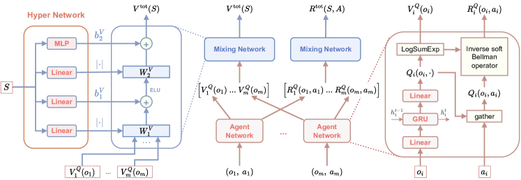
Figure 4. An overview of our network architecture; The mixing and hyper-networks of $R^{tot}$ are similar to those of $V^{tot}$.

B.2. Experimental Settings

Each environment has different a observation space, state dimension, and action space. Therefore, we use different hyper-parameters on each task to try to make all algorithms work stably. Moreover, due to limitations in computing resources, especially random access memory, we reduce the buffer size to 5000 on two hardest tasks, Miner and SMACv2, to be more efficient in running time with parallel workers. More details are available in Table 2. We use four High-Performance Computing (HPC) clusters for training and evaluating all tasks. Specifically, each HPC cluster has a workload with an NVIDIA L40 GPU 48 GB GDDR6, 32 Intel-CPU cores, and 100GB RAM. In terms of model architecture, Figure 4 shows our proposed model structure with mixing networks based on QMIX algorithm.

Table 2. Hyper-parameters.

Arguments	MPEs	Miner	SMACv2
Max training steps	100000	1000000
Evaluate times	32
Buffer size	100000	5000
Learning rate	2e-5	5e-4
Batch size	128
Hidden dim	128
Gamma	0.99
Target update frequency	4
Number of random seeds	4

B.3. Experimental Details

In this section, we present in detail experimental results for SMACv2, Miner, and MPE tasks, with varying numbers of expert demonstrations.

Table 3. Results on SMACv2, the number of expert trajectories is: 128

Methods	Protoss		Terran		Zerg		Average
	5_vs_5	10_vs_10	5_vs_5	10_vs_10	5_vs_5	10_vs_10
IIQ	9.1%	1.2%	6.5%	1.2%	2.8%	0.8%	3.6%
IQVDN	6.1%	0.2%	7.8%	0.5%	3.9%	0.4%	3.1%
MASQIL	0.3%	0.0%	0.3%	0.0%	1.4%	0.0%	0.3%
MAGAIL	0.6%	0.0%	0.0%	0.0%	3.3%	1.7%	0.9%
MIFQ (ours)	15.9%	16.8%	25.1%	0.0%	2.0%	12.5%	12.0%
Expert	86.7%	90.3%	81.7%	81.7%	73.5%	76.3%	81.7%

Table 4. Results on SMACv2, the number of expert trajectories is: 256

Methods	Protoss		Terran		Zerg		Average
	5_vs_5	10_vs_10	5_vs_5	10_vs_10	5_vs_5	10_vs_10
IIQ	11.4%	2.7%	6.7%	2.4%	9.1%	2.7%	5.8%
IQVDN	11.9%	1.6%	15.8%	1.3%	3.9%	2.0%	6.1%
MASQIL	1.0%	0.1%	0.0%	0.0%	1.6%	1.4%	0.7%
MAGAIL	13.1%	17.9%	0.5%	0.0%	4.3%	1.5%	6.2%
MIFQ (ours)	35.8%	32.7%	26.9%	0.0%	12.8%	14.6%	20.5%
Expert	86.7%	90.3%	81.7%	81.7%	73.5%	76.3%	81.7%

Table 5. Results on SMACv2, the number of expert trajectories is: 512

Methods	Protoss		Terran		Zerg		Average
	5_vs_5	10_vs_10	5_vs_5	10_vs_10	5_vs_5	10_vs_10
IIQ	17.7%	7.0%	14.3%	5.1%	9.0%	4.9%	9.7%
IQVDN	18.8%	8.1%	15.6%	15.1%	10.2%	2.1%	11.7%
MASQIL	0.1%	0.7%	2.5%	0.5%	12.8%	1.8%	3.1%
MAGAIL	1.6%	18.2%	14.6%	0.0%	14.8%	1.4%	8.4%
MIFQ (ours)	41.7%	37.8%	41.2%	0.0%	29.1%	34.7%	30.8%
Expert	86.7%	90.3%	81.7%	81.7%	73.5%	76.3%	81.7%

Table 6. Results on SMACv2, the number of expert trajectories is: 1024

Methods	Protoss		Terran		Zerg		Average
	5_vs_5	10_vs_10	5_vs_5	10_vs_10	5_vs_5	10_vs_10
IIQ	23.4%	13.5%	21.6%	9.6%	9.9%	12.0%	15.0%
IQVDN	20.1%	25.1%	22.5%	20.2%	9.1%	9.3%	17.7%
MASQIL	3.8%	3.9%	0.1%	2.4%	9.8%	2.0%	3.7%
MAGAIL	46.1%	26.0%	0.5%	0.0%	30.5%	0.5%	17.3%
MIFQ (ours)	50.3%	52.7%	51.9%	0.1%	37.0%	44.7%	39.4%
Expert	86.7%	90.3%	81.7%	81.7%	73.5%	76.3%	81.7%

Table 7. Results on SMACv2, the number of expert trajectories is: 2048

Methods	Protoss		Terran		Zerg		Average
	5_vs_5	10_vs_10	5_vs_5	10_vs_10	5_vs_5	10_vs_10
IIQ	24.2%	15.0%	17.8%	24.3%	13.0%	18.2%	18.7%
IQVDN	29.9%	25.9%	31.6%	37.9%	18.0%	14.1%	26.2%
MASQIL	41.0%	41.9%	13.7%	0.0%	19.9%	21.4%	23.0%
MAGAIL	51.7%	45.1%	28.7%	0.0%	32.7%	45.5%	33.9%
MIFQ (ours)	61.9%	47.1%	54.2%	45.7%	44.4%	47.0%	50.1%
Expert	86.7%	90.3%	81.7%	81.7%	73.5%	76.3%	81.7%

Table 8. Results on SMACv2, the number of expert trajectories is: 4096

Methods	Protoss		Terran		Zerg		Average
	5_vs_5	10_vs_10	5_vs_5	10_vs_10	5_vs_5	10_vs_10
BC	20.2%	4.6%	13.1%	5.2%	9.6%	5.1%	9.6%
IIQ	24.5%	16.2%	21.6%	15.1%	16.9%	16.4%	18.5%
IQVDN	37.1%	38.0%	28.5%	32.7%	20.6%	16.4%	28.9%
MASQIL	46.4%	37.7%	25.5%	0.5%	13.4%	27.7%	25.2%
MAGAIL	41.2%	29.7%	13.4%	0.8%	19.4%	33.1%	22.9%
MIFQ (ours)	63.2%	62.3%	57.6%	54.1%	48.8%	50.7%	56.1%
Expert	86.7%	90.3%	81.7%	81.7%	73.5%	76.3%	81.7%

Table 9. Results on Miner, the number of expert trajectories is: 128

Methods	Miner			Average
	easy	medium	hard
IIQ	6.0%	3.4%	1.5%	3.6%
IQVDN	3.2%	5.1%	2.5%	3.6%
MASQIL	13.2%	11.9%	7.0%	10.7%
MAGAIL	11.8%	11.7%	6.2%	9.9%
MIFQ (ours)	10.0%	10.6%	5.1%	8.6%
Expert	82.4%	74.9%	69.8%	75.7%

Table 10. Results on Miner, the number of expert trajectories is: 256

Methods	Miner			Average
	easy	medium	hard
IIQ	10.1%	5.8%	4.1%	6.7%
IQVDN	7.1%	5.3%	3.3%	5.2%
MASQIL	23.9%	13.5%	10.7%	16.0%
MAGAIL	20.1%	17.0%	9.5%	15.5%
MIFQ (ours)	20.6%	16.3%	8.0%	15.0%
Expert	82.4%	74.9%	69.8%	75.7%

Table 11. Results on Miner, the number of expert trajectories is: 512

Methods	Miner			Average
	easy	medium	hard
IIQ	11.1%	8.7%	5.6%	8.5%
IQVDN	11.0%	6.4%	3.8%	7.1%
MASQIL	28.6%	15.9%	15.7%	20.1%
MAGAIL	27.2%	22.2%	12.8%	20.7%
MIFQ (ours)	25.3%	17.1%	12.1%	18.2%
Expert	82.4%	74.9%	69.8%	75.7%

Table 12. Results on Miner, the number of expert trajectories is: 1024

Methods	Miner			Average
	easy	medium	hard
IIQ	18.4%	7.5%	5.9%	10.6%
IQVDN	8.7%	5.0%	6.9%	6.9%
MASQIL	34.3%	24.7%	18.3%	25.8%
MAGAIL	31.5%	22.6%	14.7%	22.9%
MIFQ (ours)	33.3%	23.1%	17.1%	24.5%
Expert	82.4%	74.9%	69.8%	75.7%

Table 13. Results on Miner, the number of expert trajectories is: 2048

Methods	Miner			Average
	easy	medium	hard
IIQ	19.9%	8.9%	7.5%	12.1%
IQVDN	12.8%	8.0%	6.2%	9.0%
MASQIL	34.8%	27.1%	19.8%	27.2%
MAGAIL	30.7%	25.6%	17.9%	24.7%
MIFQ (ours)	39.6%	32.5%	21.0%	31.0%
Expert	82.4%	74.9%	69.8%	75.7%

Table 14. Results on Miner, the number of expert trajectories is: 4096

Methods	Miner			Average
	easy	medium	hard
BC	26.9%	21.7%	13.3%	20.6%
IIQ	14.7%	8.0%	6.0%	9.6%
IQVDN	18.3%	12.1%	9.7%	13.4%
MASQIL	31.9%	21.6%	18.5%	24.0%
MAGAIL	34.0%	25.0%	20.1%	26.4%
MIFQ (ours)	44.9%	35.6%	24.7%	35.0%
Expert	82.4%	74.9%	69.8%	75.7%

Table 15. Results on MPEs, the number of expert trajectories is: 1

Methods	Simple			Average
	reference	spread	speaker_listener
IIQ	-27.8	-38.4	-64.9	-43.7
MASQIL	-45.2	-56.4	-128.3	-76.6
MAGAIL	-50.9	-43.9	-101.6	-65.5
MIFQ (ours)	-49.5	-37.5	-78.5	-55.2
Expert	-17.2	-10.7	-19.7	-15.8

Table 16. Results on MPEs, the number of expert trajectories is: 2

Methods	Simple			Average
	reference	spread	speaker_listener
IIQ	-28.5	-34.5	-80.6	-47.9
MASQIL	-48.4	-54.2	-114.3	-72.3
MAGAIL	-47.3	-42.7	-104.1	-64.7
MIFQ (ours)	-45.9	-38.9	-88.6	-57.8
Expert	-17.2	-10.7	-19.7	-15.8

Table 17. Results on MPEs, the number of expert trajectories is: 4

Methods	Simple			Average
	reference	spread	speaker_listener
IIQ	-29.0	-33.1	-67.4	-43.1
MASQIL	-47.9	-44.5	-112.0	-68.1
MAGAIL	-49.4	-43.3	-90.2	-61.0
MIFQ (ours)	-46.1	-37.3	-119.6	-67.6
Expert	-17.2	-10.7	-19.7	-15.8

Table 18. Results on MPEs, the number of expert trajectories is: 8

Methods	Simple			Average
	reference	spread	speaker_listener
IIQ	-27.7	-27.7	-62.7	-39.4
MASQIL	-43.7	-49.6	-110.5	-68.0
MAGAIL	-41.2	-43.9	-99.5	-61.5
MIFQ (ours)	-44.1	-34.3	-61.1	-46.5
Expert	-17.2	-10.7	-19.7	-15.8

Table 19. Results on MPEs, the number of expert trajectories is: 16

Methods	Simple			Average
	reference	spread	speaker_listener
IIQ	-27.9	-27.2	-57.2	-37.4
MASQIL	-44.2	-45.8	-128.5	-72.8
MAGAIL	-42.4	-40.4	-135.1	-72.6
MIFQ (ours)	-51.8	-31.5	-42.1	-41.8
Expert	-17.2	-10.7	-19.7	-15.8

Table 20. Results on MPEs, the number of expert trajectories is: 32

Methods	Simple			Average
	reference	spread	speaker_listener
IIQ	-25.7	-27.4	-46.3	-33.1
MASQIL	-45.4	-34.7	-105.9	-62.0
MAGAIL	-36.3	-34.1	-133.5	-68.0
MIFQ (ours)	-31.8	-25.2	-36.7	-31.3
Expert	-17.2	-10.7	-19.7	-15.8

Table 21. Results on MPEs, the number of expert trajectories is: 64

Methods	Simple			Average
	reference	spread	speaker_listener
IIQ	-23.9	-24.5	-48.5	-32.3
MASQIL	-37.1	-32.2	-146.3	-71.8
MAGAIL	-41.7	-32.1	-117.6	-63.8
MIFQ (ours)	-24.4	-23.9	-33.5	-27.3
Expert	-17.2	-10.7	-19.7	-15.8

Table 22. Results on MPEs, the number of expert trajectories is: 128

Methods	Simple			Average
	reference	spread	speaker_listener
BC	-25.6	-23.6	-28.6	-25.9
IIQ	-23.8	-24.4	-47.3	-31.8
IQVDN	-23.2	-24.1	-46.6	-31.3
MASQIL	-49.6	-28.4	-148.5	-75.5
MAGAIL	-41.3	-30.3	-136.5	-69.4
MIFQ (ours)	-23.0	-23.3	-31.3	-25.8
Expert	-17.2	-10.7	-19.7	-15.8

References

- (1)
- Abbeel and Ng (2004) Pieter Abbeel and Andrew Y Ng. 2004. Apprenticeship learning via inverse reinforcement learning. In Proceedings of the twenty-first international conference on Machine learning. 1.
- Arora and Doshi (2021) Saurabh Arora and Prashant Doshi. 2021. A survey of inverse reinforcement learning: Challenges, methods and progress. Artificial Intelligence 297 (2021), 103500.
- Barrett et al. (2017) Samuel Barrett, Avi Rosenfeld, Sarit Kraus, and Peter Stone. 2017. Making friends on the fly: Cooperating with new teammates. Artificial Intelligence 242 (2017), 132–171.
- Bhattacharyya et al. (2018) Raunak P Bhattacharyya, Derek J Phillips, Blake Wulfe, Jeremy Morton, Alex Kuefler, and Mykel J Kochenderfer. 2018. Multi-agent imitation learning for driving simulation. In 2018 IEEE/RSJ International Conference on Intelligent Robots and Systems (IROS). IEEE, 1534–1539.
- Bogert and Doshi (2014) Kenneth Bogert and Prashant Doshi. 2014. Multi-robot inverse reinforcement learning under occlusion with interactions. In Proceedings of the 2014 international conference on Autonomous agents and multi-agent systems. 173–180.
- Boyd and Vandenberghe (2004) Stephen P Boyd and Lieven Vandenberghe. 2004. Convex optimization. Cambridge university press.
- Bui et al. (2023) The Viet Bui, Tien Mai, and Thanh Hong Nguyen. 2023. Mimicking To Dominate: Imitation Learning Strategies for Success in Multiagent Competitive Games. arXiv preprint arXiv:2308.10188 (2023).
- Claus and Boutilier (1998) Caroline Claus and Craig Boutilier. 1998. The dynamics of reinforcement learning in cooperative multiagent systems. AAAI/IAAI 1998, 746-752 (1998), 2.
- de Witt et al. (2020) Christian Schroeder de Witt, Tarun Gupta, Denys Makoviichuk, Viktor Makoviychuk, Philip HS Torr, Mingfei Sun, and Shimon Whiteson. 2020. Is independent learning all you need in the starcraft multi-agent challenge? arXiv preprint arXiv:2011.09533 (2020).
- Dugas et al. (2009) Charles Dugas, Yoshua Bengio, François Bélisle, Claude Nadeau, and René Garcia. 2009. Incorporating Functional Knowledge in Neural Networks. Journal of Machine Learning Research 10, 6 (2009).
- Ellis et al. (2022) Benjamin Ellis, Skander Moalla, Mikayel Samvelyan, Mingfei Sun, Anuj Mahajan, Jakob N Foerster, and Shimon Whiteson. 2022. SMACv2: An improved benchmark for cooperative multi-agent reinforcement learning. arXiv preprint arXiv:2212.07489 (2022).
- Finn et al. (2016) Chelsea Finn, Paul Christiano, Pieter Abbeel, and Sergey Levine. 2016. A connection between generative adversarial networks, inverse reinforcement learning, and energy-based models. arXiv preprint arXiv:1611.03852 (2016).
- Foerster et al. (2018) Jakob Foerster, Gregory Farquhar, Triantafyllos Afouras, Nantas Nardelli, and Shimon Whiteson. 2018. Counterfactual multi-agent policy gradients. In Proceedings of the AAAI conference on artificial intelligence, Vol. 32.
- FPT (2020) FPT. 2020. FPT Reinforcement Learning Competition. https://codelearn.io/game/detail/2212875#ai-game-summary.
- Fu et al. (2017) Justin Fu, Katie Luo, and Sergey Levine. 2017. Learning robust rewards with adversarial inverse reinforcement learning. arXiv preprint arXiv:1710.11248 (2017).
- Garg et al. (2021) Divyansh Garg, Shuvam Chakraborty, Chris Cundy, Jiaming Song, and Stefano Ermon. 2021. Iq-learn: Inverse soft-q learning for imitation. Advances in Neural Information Processing Systems 34 (2021), 4028–4039.
- Goodfellow et al. (2014) Ian Goodfellow, Jean Pouget-Abadie, Mehdi Mirza, Bing Xu, David Warde-Farley, Sherjil Ozair, Aaron Courville, and Yoshua Bengio. 2014. Generative adversarial nets. Advances in neural information processing systems 27 (2014).
- Ha et al. (2017) David Ha, Andrew M. Dai, and Quoc V. Le. 2017. HyperNetworks. In International Conference on Learning Representations. https://openreview.net/forum?id=rkpACe1lx
- Hawke et al. (2020) Jeffrey Hawke, Richard Shen, Corina Gurau, Siddharth Sharma, Daniele Reda, Nikolay Nikolov, Przemysław Mazur, Sean Micklethwaite, Nicolas Griffiths, Amar Shah, et al. 2020. Urban driving with conditional imitation learning. In 2020 IEEE International Conference on Robotics and Automation (ICRA). IEEE, 251–257.
- Ho and Ermon (2016) Jonathan Ho and Stefano Ermon. 2016. Generative adversarial imitation learning. Advances in neural information processing systems 29 (2016).
- Hu et al. (1998) Junling Hu, Michael P Wellman, et al. 1998. Multiagent reinforcement learning: theoretical framework and an algorithm.. In ICML, Vol. 98. 242–250.
- Jeon et al. (2020) Wonseok Jeon, Paul Barde, Derek Nowrouzezahrai, and Joelle Pineau. 2020. Scalable and sample-efficient multi-agent imitation learning. In Proceedings of the Workshop on Artificial Intelligence Safety, co-located with 34th AAAI Conference on Artificial Intelligence, SafeAI@ AAAI.
- Kostrikov et al. (2019) Ilya Kostrikov, Ofir Nachum, and Jonathan Tompson. 2019. Imitation learning via off-policy distribution matching. arXiv preprint arXiv:1912.05032 (2019).
- Kraemer and Banerjee (2016) Landon Kraemer and Bikramjit Banerjee. 2016. Multi-agent reinforcement learning as a rehearsal for decentralized planning. Neurocomputing 190 (2016), 82–94.
- Le et al. (2017) Hoang M Le, Yisong Yue, Peter Carr, and Patrick Lucey. 2017. Coordinated multi-agent imitation learning. In International Conference on Machine Learning. PMLR, 1995–2003.
- Le Mero et al. (2022) Luc Le Mero, Dewei Yi, Mehrdad Dianati, and Alexandros Mouzakitis. 2022. A survey on imitation learning techniques for end-to-end autonomous vehicles. IEEE Transactions on Intelligent Transportation Systems 23, 9 (2022), 14128–14147.
- Lin et al. (2014) Xiaomin Lin, Peter A Beling, and Randy Cogill. 2014. Multi-agent inverse reinforcement learning for zero-sum games. arXiv preprint arXiv:1403.6508 (2014).
- Littman (1994) Michael L Littman. 1994. Markov games as a framework for multi-agent reinforcement learning. In Machine learning proceedings 1994. Elsevier, 157–163.
- Lowe et al. (2017) Ryan Lowe, Yi I Wu, Aviv Tamar, Jean Harb, OpenAI Pieter Abbeel, and Igor Mordatch. 2017. Multi-agent actor-critic for mixed cooperative-competitive environments. Advances in neural information processing systems 30 (2017).
- Oliehoek et al. (2016) Frans A Oliehoek, Christopher Amato, et al. 2016. A concise introduction to decentralized POMDPs. Vol. 1. Springer.
- Oliehoek et al. (2008) Frans A Oliehoek, Matthijs TJ Spaan, and Nikos Vlassis. 2008. Optimal and approximate Q-value functions for decentralized POMDPs. Journal of Artificial Intelligence Research 32 (2008), 289–353.
- Pomerleau (1991) Dean A Pomerleau. 1991. Efficient training of artificial neural networks for autonomous navigation. Neural computation 3, 1 (1991), 88–97.
- Rashid et al. (2020) Tabish Rashid, Mikayel Samvelyan, Christian Schroeder De Witt, Gregory Farquhar, Jakob Foerster, and Shimon Whiteson. 2020. Monotonic value function factorisation for deep multi-agent reinforcement learning. The Journal of Machine Learning Research 21, 1 (2020), 7234–7284.
- Reddy et al. (2019) Siddharth Reddy, Anca D Dragan, and Sergey Levine. 2019. Sqil: Imitation learning via reinforcement learning with sparse rewards. arXiv preprint arXiv:1905.11108 (2019).
- Reddy et al. (2012) Tummalapalli Sudhamsh Reddy, Vamsikrishna Gopikrishna, Gergely Zaruba, and Manfred Huber. 2012. Inverse reinforcement learning for decentralized non-cooperative multiagent systems. In 2012 IEEE International Conference on Systems, Man, and Cybernetics (SMC). IEEE, 1930–1935.
- Ross and Bagnell (2010) Stéphane Ross and Drew Bagnell. 2010. Efficient reductions for imitation learning. In Proceedings of the thirteenth international conference on artificial intelligence and statistics. JMLR Workshop and Conference Proceedings, 661–668.
- Ross et al. (2011) Stéphane Ross, Geoffrey Gordon, and Drew Bagnell. 2011. A reduction of imitation learning and structured prediction to no-regret online learning. In Proceedings of the fourteenth international conference on artificial intelligence and statistics. JMLR Workshop and Conference Proceedings, 627–635.
- Samvelyan et al. (2019) Mikayel Samvelyan, Tabish Rashid, Christian Schroeder De Witt, Gregory Farquhar, Nantas Nardelli, Tim GJ Rudner, Chia-Man Hung, Philip HS Torr, Jakob Foerster, and Shimon Whiteson. 2019. The starcraft multi-agent challenge. arXiv preprint arXiv:1902.04043 (2019).
- Shah et al. (2022) Syed Ihtesham Hussain Shah, Antonio Coronato, Muddasar Naeem, and Giuseppe De Pietro. 2022. Learning and assessing optimal dynamic treatment regimes through cooperative imitation learning. IEEE Access 10 (2022), 78148–78158.
- Song et al. (2018) Jiaming Song, Hongyu Ren, Dorsa Sadigh, and Stefano Ermon. 2018. Multi-agent generative adversarial imitation learning. Advances in neural information processing systems 31 (2018).
- Šošić et al. (2016) Adrian Šošić, Wasiur R KhudaBukhsh, Abdelhak M Zoubir, and Heinz Koeppl. 2016. Inverse reinforcement learning in swarm systems. arXiv preprint arXiv:1602.05450 (2016).
- Sunehag et al. (2017) Peter Sunehag, Guy Lever, Audrunas Gruslys, Wojciech Marian Czarnecki, Vinicius Zambaldi, Max Jaderberg, Marc Lanctot, Nicolas Sonnerat, Joel Z Leibo, Karl Tuyls, et al. 2017. Value-decomposition networks for cooperative multi-agent learning. arXiv preprint arXiv:1706.05296 (2017).
- Wang et al. (2020) Lu Wang, Wenchao Yu, Xiaofeng He, Wei Cheng, Martin Renqiang Ren, Wei Wang, Bo Zong, Haifeng Chen, and Hongyuan Zha. 2020. Adversarial Cooperative Imitation Learning for Dynamic Treatment Regimes. In Proceedings of The Web Conference 2020. 1785–1795.
- Yu et al. (2022) Chao Yu, Akash Velu, Eugene Vinitsky, Jiaxuan Gao, Yu Wang, Alexandre Bayen, and Yi Wu. 2022. The surprising effectiveness of ppo in cooperative multi-agent games. Advances in Neural Information Processing Systems 35 (2022), 24611–24624.
- Yu et al. (2019) Lantao Yu, Jiaming Song, and Stefano Ermon. 2019. Multi-agent adversarial inverse reinforcement learning. In International Conference on Machine Learning. PMLR, 7194–7201.
- Zhou et al. (2021) Jinyun Zhou, Rui Wang, Xu Liu, Yifei Jiang, Shu Jiang, Jiaming Tao, Jinghao Miao, and Shiyu Song. 2021. Exploring imitation learning for autonomous driving with feedback synthesizer and differentiable rasterization. In 2021 IEEE/RSJ International Conference on Intelligent Robots and Systems (IROS). IEEE, 1450–1457.
- Ziebart et al. (2008) Brian D Ziebart, Andrew L Maas, J Andrew Bagnell, Anind K Dey, et al. 2008. Maximum entropy inverse reinforcement learning.. In Aaai, Vol. 8. Chicago, IL, USA, 1433–1438.